climatology of extreme rainfall from rain gauges and...
TRANSCRIPT

Climatology of extreme rainfall from rain
gauges and weather radar
Aart Overeem

Thesis committee
Thesis supervisor
Prof. dr. ir. R. Uijlenhoet
Professor of Hydrology and Quantitative Water Management
Wageningen University, the Netherlands
Thesis co-supervisors
Dr. I. Holleman
Senior Scientist, KNMI, De Bilt, the Netherlands
Dr. T. A. Buishand
Senior Scientist, KNMI, De Bilt, the Netherlands
Other members
Prof. dr. A. A. M. Holtslag, Wageningen University, the Netherlands
Prof. dr. ir. M. F. P. Bierkens, Utrecht University, the Netherlands
Prof. C. G. Collier, University of Leeds, United Kingdom
Prof. C. W. Anderson, University of Sheffield, United Kingdom
This research was conducted under the auspices of the SENSE Research School.

Climatology of extreme rainfall from rain
gauges and weather radar
Aart Overeem
Thesis
submitted in partial fulfilment of the requirements for the degree of doctor
at Wageningen University
by the authority of the Rector Magnificus
Prof. dr. M. J. Kropff,
in the presence of the
Thesis Committee appointed by the Doctorate Board
to be defended in public
on Friday 4 December 2009
at 1:30 PM in the Aula

Aart Overeem
Climatology of extreme rainfall from rain gauges and weather radar, xii+132 pages.
In Dutch: Klimatologie van extreme neerslag uit regenmeters en weerradar, xii+132 blz.
Thesis Wageningen University, Wageningen, NL (2009)
With references, with summaries in Dutch and English
ISBN 978-90-8585-517-0

vAbstract
Extreme rainfall events can have a large impact on society and can lead to loss of life and
property. Therefore, a reliable climatology of extreme rainfall is of importance, for instance,
for the design of hydraulic structures. Such a climatology can be obtained by abstracting
maxima from long rainfall records. Subsequently, a probability distribution is fitted to the
selected maxima, so that rainfall depths can be estimated for a chosen return period, which
can be longer than the rainfall record. In this thesis, the Generalized Extreme Value (GEV)
distribution is used to model annual rainfall maxima.
Using a new methodology, rain gauge data from 12 stations in the Netherlands are em-
ployed to derive rainfall depth-duration-frequency (DDF) curves, which describe rainfall
depth as a function of duration for given return periods. Often, uncertainties are not in-
corporated in the design of hydraulic structures, which can lead to a risk of under design.
Therefore, uncertainties in the DDF curves are estimated as well.
Weather radars are widely used in real-time quantitative precipitation estimation over
large areas with high temporal and spatial resolutions not achieved by conventional rain
gauge networks. A 10-year radar-based climatology of rainfall depths for durations of 15
min to 24 h is derived for the Netherlands. Since radar data can be vulnerable to a number
of errors, they are adjusted using rain gauges. Verification shows that the radar data set has
a high quality.
In general, only few digitized time series from rain gauges are available for subdaily du-
rations. This hampers the study of regional variability in extreme rainfall and the estimation
of extreme areal rainfall, which can be overcome by using weather radar. The climatological
radar rainfall data set is utilized to obtain annual rainfall maxima for durations of 15 min to
24 h and the size of a radar pixel. GEV distributions are fitted to these annual maxima. For
most durations, significant regional differences in extreme rainfall in the Netherlands are
found. Subsequently, rainfall DDF curves are constructed. The radar-based extreme rainfall
statistics are in good agreement with those obtained from rain gauges, although an under-
estimation is found for short durations. The uncertainties in radar-based DDF curves are
small for short durations and become rather large for long durations.
Employing the climatological radar data set, annual maxima are obtained for area sizes
ranging from a radar pixel to approximately 1700 km2. A single equation is derived from
which rainfall depths for a chosen return period and area size can be calculated for different
durations: the areal DDF curve. Extreme areal rainfall statistics based on rain gauge data
agree well with those derived from radar data.
The main result of this thesis is that, after adjustment with rain gauges, weather radar
data can be used to derive a climatology of extreme (areal) rainfall including the uncertain-
ties and can be used to study regional differences in extreme rainfall.

vi Samenvatting
Extreme neerslaggebeurtenissen hebben een grote invloed op de maatschappij en kunnen
leiden tot materiele schade en slachtoffers. Daarom is een betrouwbare klimatologie van ex-
treme neerslag belangrijk, bijvoorbeeld voor het ontwerp van afvoersystemen. Een derge-
lijke klimatologie kan worden verkregen door jaarmaxima te selecteren uit lange neerslag-
reeksen. Vervolgens wordt een kansverdeling aangepast aan de geselecteerde jaarmaxima,
zodat neerslaghoeveelheden kunnen worden geschat voor een gekozen herhalingstijd, die
langer kan zijn dan de neerslagreeks. In dit proefschrift worden jaarmaxima gemodelleerd
met de Gegeneraliseerde Extreme Waarden (GEV) verdeling.
Met een nieuwe methode worden regenduurlijnen afgeleid op basis van 12 neerslagreek-
sen uit Nederland. Regenduurlijnen geven de hoeveelheid neerslag weer als functie van de
duur voor gegeven herhalingstijden. Vaak worden onzekerheden niet meegenomen in het
ontwerp van afvoersystemen, met het risico op een te krap bemeten systeem. Daarom wor-
den ook de onzekerheden in de regenduurlijnen geschat.
Weerradars worden wijd en zijd gebruikt voor directe kwantitatieve neerslagschattingen
over grote gebieden met hoge temporele en ruimtelijke resoluties die niet worden gehaald
met traditionele regenmeternetwerken. Een 10-jarige op radar gebaseerde klimatologie van
neerslaghoeveelheden wordt vervaardigd voor duren van 15 min tot 24 uur voor Nederland.
Omdat radardata gevoelig kunnen zijn voor een aantal fouten, worden ze gecorrigeerd met
regenmeters. Verificatie toont de goede kwaliteit van de radar dataset aan.
In het algemeen zijn er voor duren korter dan een dag maar weinig gedigitaliseerde
tijdreeksen van regenmeters. Dit belemmert de studie naar regionale verschillen in extre-
me neerslag en het schatten van extreme gebiedsneerslag. Weerradar kan hier uitkomst
bieden. Jaarmaxima worden geselecteerd uit de klimatologische radar dataset voor duren
van 15 min tot 24 uur en een gebiedsgrootte van een radar pixel. De jaarmaxima worden
gemodelleerd met GEV verdelingen. Voor de meeste duren worden significante regionale
verschillen in extreme neerslag gevonden voor Nederland. Vervolgens worden regenduur-
lijnen afgeleid. De op radar gebaseerde extreme neerslagstatistieken zijn in goede overeen-
stemming met die gebaseerd op regenmeters, alhoewel een onderschatting wordt gevonden
voor korte duren. De onzekerheden in de op radar gebaseerde regenduurlijnen zijn klein
voor korte duren en worden vrij groot voor lange duren.
Gebruikmakend van de klimatologische radar dataset worden jaarmaxima geselecteerd
voor gebiedsgroottes van een radar pixel tot ongeveer 1700 km2. De neerslaghoeveelheden
kunnen worden berekend uit een vergelijking voor een gekozen herhalingstijd en gebieds-
grootte voor verschillende duren: de gebiedsregenduurlijn. Extreme gebiedsneerslagstatis-
tieken op basis van regenmeterdata komen goed overeen met die uit radardata.
Het belangrijkste resultaat van dit proefschrift is dat, na correctie met regenmeterdata,
weerradardata geschikt zijn om een extreme neerslagklimatologie af te leiden, inclusief
onzekerheden, en bruikbaar zijn voor de bestudering van regionale verschillen in extreme
neerslag.

viiVoorwoord
Na als meteoroloog te zijn afgestudeerd in november 2002, deed de meteorologische sec-
tor alsof hij conjunctuurgevoelig was, waardoor er maar weinig vacatures waren. Na een
periode van administratief uitzendwerk was het gelukkig mogelijk om verder te studeren
in de richting van de hydrologie. De enthousiaste colleges van Bram van Putten (Wagenin-
gen Universiteit) over hydrologische statistiek wekten mijn interesse om bij hem een af-
studeervak te doen over neerslagstatistiek. En tijdens een afstudeervak over statistische
waterstandsverwachtingen van de Rijn en hun onzekerheden bij Paul Torfs (Wageningen
Universiteit) kwam ik in aanraking met het statistische programma 1 (nog bedankt Paul!).
Van deze extra bagage zou ik later nog veel profijt blijken te hebben en zij is, achteraf gezien,
misschien ook wel nodig geweest om gemotiveerd en met voldoende achtergrondkennis aan
dit promotieonderzoek te beginnen. Zo konden met vrijwel alle figuren in dit proefschrift
worden gemaakt en de extreme-waarden analyses worden uitgevoerd. In het voorjaar van
2005 kwam dan die vacature bij het KNMI waar ik niet om heen kon. De inhoud van deze
promotieplaats zat op het grensvlak van meteorologie en hydrologie en de statistiek speelde
(toevallig?) een hoofdrol. Echter, de weerradar was voor mij nog onontgonnen terrein. Het
KNMI was mij al in positieve zin bekend van een afstudeervak uit 2002. Wel had ik aan-
vankelijk nog enige twijfels of een vierjarig programma wat voor mij zou zijn, maar die
verdwenen, mede door advies van Bram, als sneeuw voor de zon. Achteraf gezien is het,
wat mij betreft (...), de juiste keuze gebleken.
Hoe is dit promotieonderzoek eigenlijk tot stand gekomen? Welnu, dit promotieonderzoek
is mogelijk gemaakt door de Staatssecretaris van het Ministerie van Verkeer en Waterstaat.
Ter gelegenheid van het 150-jarig bestaan van het KNMI werd financiering gegeven voor
vier jubileum onderzoekers in opleiding. Na een interne evaluatieronde werd besloten dat
de, statistisch gezien, onafhankelijk van elkaar ingediende voorstellen van Adri Buishand en
Iwan Holleman samengevoegd moesten worden. Dit leidde tot een project waarin een brug
werd geslagen tussen de “statistiekwereld” en de “radarwereld”, alsmede tussen de afde-
ling Klimaatdata en -advies van de sector Klimaat en Seismologie en de afdeling Onderzoek
van de sector Weer.
De eersten die ik wil bedanken zijn mijn copromotors Adri Buishand en Iwan Holleman
en mijn promotor Remko Uijlenhoet. Adri, ik heb veel geleerd van je precisie en kennis
en wil je hartelijk bedanken voor je grote inzet. Iwan, je hebt me de afgelopen vier jaar
erg weten te motiveren en hield daarbij altijd de grote lijn en het einddoel voor ogen. Ook
voor jou geldt dat je veel tijd voor me had en ik wil je dan ook hartelijk bedanken voor
alle begeleiding. Uiteindelijk is gebleken dat jullie, Adri en Iwan, elkaar goed aanvulden:
door de verschillende expertises kwam ik zelden in een inhoudelijke spagaat te zitten. En
Remko, sinds het begin was je betrokken bij dit project. Ik wil je hartelijk bedanken voor
1http://www.r-project.org/

viii
je bijdrage en supervisie die onder andere uitmondde in je coauteurschap van hoofdstuk 5.
Adri, Iwan en Remko: bedankt voor de plezierige samenwerking! Zonder jullie en het goede
onderzoeksplan, was het mij nooit gelukt om alles binnen een redelijke tijd af te ronden.
Een beperkt aantal KNMI collega’s wil ik hierbij in het bijzonder noemen. Hans Beekhuis,
bedankt voor het uitdragen van je radarkennis en je commentaar op hoofdstuk 1. Rudolf van
Westrhenen wil ik hartelijk bedanken voor het archiveren van de radardata op zijn werksta-
tion van 1998 tot medio 2003. Hierdoor was het mogelijk om bruikbare neerslagstatistieken
te berekenen op basis van radardata. Siebren de Haan wil ik bedanken voor zijn bestanden
die als voorbeeld dienden om dit proefschrift op te maken. Ook wil ik mijn afdelingshoofd
Gerrit Burgers bedanken voor zijn interesse en motivatie. Vele andere collega’s zijn ook
behulpzaam geweest in het beantwoorden van vragen en het leveren van data, waarvoor
dank. Verder wil ik ook mijn kamergenoot Hans de Vries bedanken voor de prettige sfeer en
je behulpzaamheid bij vragen over Linux en het opmaaksysteem LATEX. Met dat laatste is dit
proefschrift vervaardigd, dat overigens gedrukt is door A-D Druk te Zeist. In het bijzonder
nog een dankwoord voor mijn collega’s van Weer Onderzoek. De plezierige, ongedwongen
sfeer en “lunchcultuur”, waarbij het over meer dan weer ging, heb ik altijd erg gewaardeerd.
Verder wil ik Hanneke Schuurmans (voorheen Universiteit Utrecht, nu FutureWater) be-
danken voor de -scriptjes die als basis dienden voor de visualisatie van de radarbeelden
in dit proefschrift. Ook een woord van dank aan Hidde Leijnse, Pieter Hazenberg en Remco
van de Beek (Wageningen Universiteit), Adriaan Dokter (KNMI) en wederom Hanneke voor
de uitwisseling van kennis m.b.t. weerradaronderzoek. Ook wil ik Iwan’s moeder, M. van
Rens, bedanken voor het beschikbaar stellen van de foto van wateroverlast op de omslag
van dit proefschrift. Thanks to Markus Peura (Finnish Meteorological Institute) for provid-
ing Figure 1.3.
In de privesfeer hebben een aantal familieleden, vrienden & vriendinnen regelmatig een
luisterend oor geboden, wat ik altijd erg waardeerde. Het zou me niets verbazen als jullie
er weleens moe van werden... Een aantal van hen wil ik hier expliciet noemen. Ten eerste
mijn ouders. Bedankt dat jullie me altijd hebben gestimuleerd om te studeren en dat ook
mogelijk hebben gemaakt! Verder wil ik mijn broer Edwin, mijn paranimfen Luuc en Stefan,
Gert-Jan & Celia en Peter L. bedanken voor hun steun. Evenals een bijzonder persoon die er
in het eindtraject pas bij kwam: Annemarie. Ten slotte, dank aan God!
Aart Overeem
Zeist, oktober 2009

Contents
1 Introduction 1
1.1 Motivation 2
1.1.1 Importance of a climatology of extreme rainfall 2
1.1.2 Recent studies of extreme rainfall statistics for the Netherlands 3
1.1.3 Potential of weather radar 4
1.1.4 Research questions 7
1.2 Quantitative precipitation estimation from weather radar 8
1.2.1 Pulses, echo powers and sampling 8
1.2.2 The radar equation 11
1.2.3 From radar reflectivity factor to rainfall intensity 13
1.3 Outline 14
2 Rainfall depth-duration-frequency curves and their uncertainties 17
2.1 Introduction 18
2.2 Rainfall data 19
2.2.1 Rain gauge networks 19
2.2.2 Adjustment of automatic gauge data 21
2.3 Regional variability in extreme rainfall statistics 21
2.3.1 Fitting a GEV distribution 22
2.3.2 Regional variability in GEV parameters 24
2.4 Regional estimation and modelling of GEV parameters 25
2.4.1 Estimated GEV parameters for individual durations 25
2.4.2 Correlations of estimated GEV parameters 27
2.4.3 GEV parameters as a function of duration 28
2.5 Construction of rainfall DDF curves and their uncertainties 31
2.5.1 Derivation of DDF curves 31
2.5.2 Modelling uncertainty in DDF curves 31
2.6 Conclusions 33
3 Derivation of a 10-year radar-based climatology of rainfall 35
3.1 Introduction 36
3.2 Radar and rain gauge data 38
ix

x
3.2.1 Radar data 38
3.2.2 Rain gauge networks 40
3.3 Adjustment of radar-based rainfall accumulations 41
3.3.1 Correction for occultation per radar 41
3.3.2 Daily VPR and bias adjustment per radar (VPR adjustment) 41
3.3.3 Compositing of accumulation images 43
3.3.4 Daily spatial adjustment of composites (S adjustment) 43
3.3.5 Hourly mean-field bias adjustment of composites (MFB adjustment) 44
3.3.6 Spatial adjustment of MFB-adjusted composites (MFBS adjustment) 45
3.4 Characterization and verification of adjusted accumulations 45
3.4.1 Seasonal cycle of the VPR gradient 45
3.4.2 Verification with manual rain gauges 46
3.4.3 Verification with automatic rain gauges 48
3.5 Long-term radar rainfall statistics 50
3.5.1 Empirical exceedance probabilities 50
3.5.2 Rainfall frequency and maximum rainfall depths 52
3.5.3 Spatial correlation 53
3.6 Conclusions and recommendations 55
4 Extreme rainfall analysis and estimation of DDF curves using radar 59
4.1 Introduction 60
4.2 Radar and rain gauge data 61
4.3 Adjustment of radar-based rainfall depths 62
4.3.1 Adjustment method 62
4.3.2 Derivation of adjusted 15-min to 120-min composites 63
4.4 Characteristics of annual maxima 64
4.5 Regional variability in extreme rainfall statistics 67
4.5.1 Fitting a GEV distribution 67
4.5.2 Bootstrap samples 69
4.5.3 Test for regional variability in µ 70
4.6 Comparison of radar and rain gauge extreme rainfall statistics 75
4.7 Regional estimation and modeling of GEV parameters 76
4.7.1 Estimated GEV parameters for individual durations 76
4.7.2 GEV parameters as a function of duration 78
4.8 Construction of DDF curves and modeling their uncertainties 78
4.8.1 Derivation of DDF curves 78
4.8.2 Modeling uncertainty in DDF curves 79
4.8.3 Local DDF curves 80
4.9 Discussion and conclusions 81

xi
5 Extreme-value modeling of areal rainfall from weather radar 85
5.1 Introduction 86
5.2 Radar data 87
5.3 Extreme-value modeling of areal rainfall 88
5.3.1 Abstracting annual maxima 88
5.3.2 Fitting a GEV distribution 88
5.3.3 Bootstrap samples 91
5.4 GEV parameters as a function of duration and area size 91
5.5 Derivation of areal DDF curves and their uncertainties 94
5.6 Areal reduction factors 96
5.7 Discussion and conclusions 98
6 Conclusions and outlook 101
6.1 Summary 102
6.2 Conclusions 102
6.3 Outlook 105
6.3.1 The future of QPE 105
6.3.2 Applications of climatological radar rainfall data sets 107
Bibliography 109
A Bootstrap algorithm 121
B Maximum likelihood versus L-moments 123
C Influence of missing data on estimated GEV parameters 127
List of Publications 128
Curriculum Vitae 131

xii

Chapter 1
Introduction
Inundation due to an extreme rainfall event in Nijmegen, the Netherlands
(Courtesy of M. van Rens)
1

2 Chapter 1 — Introduction
1.1 Motivation
1.1.1 Importance of a climatology of extreme rainfall
Extreme rainfall events have a large impact on society and can lead to loss of life and prop-
erty, for instance, by causing land slides or flooding due to dike breach or dam failure. Such
events may also give rise to an exceedance of the capacity of sewer systems resulting in in-
undation of streets and basements. To prevent such hazards and nuisance proper design
criteria have to be formulated. It is up to society to decide which risk is acceptable, for
instance, how often flooding is allowed to occur. Subsequently, scientists can estimate the
discharges and rainfalls, which are used to design hydraulic structures according to the cri-
teria as laid down by law or agreement. Thus, accurate estimates of extreme rainfall depths
and discharges are of the utmost importance.
In the Netherlands, “Het nationaal bestuursakkoord water”, a covenant between the Dutch
government, provincial authorities, municipalities, and water authorities, gives design crite-
ria for the regional water system. Criteria of flooding from water systems differ with respect
to type of land use. For example, flooding from surface water is allowed to occur on aver-
age from once in 100 years for urbanized areas to once in 10 years for grassland. Because
discharge records for regional water systems are often not available, rainfall data have to be
used. In the Netherlands, most sewer systems are designed to discharge a design storm cor-
responding to a return period of approximately 2 years. More extreme events with a return
period of 10-25 years lead to inundated streets and underpasses. In addition, events with a
return period of 50 years may, for instance, result in buildings suffering water damage. For
more information, see Van Luijtelaar (2006). Urban areas and sewer systems in the Nether-
lands are particularly vulnerable to convective rainfall events with a duration shorter than
40 minutes (Zondervan, 1978). For regional water systems events lasting several hours to
days are of main concern.
This thesis focuses on the statistics of extreme rainfall for the Netherlands. These statistics
are not only relevant for design purposes in water management, such as the construction
of sewer systems (Figure 1.1), the determination of the required discharge capacity of wa-
terways or the required pumping capacity of polders. Other uses are important as well, for
example, the evaluation of hazardous weather, advice to the general public, insurance of
water damage, and, last but not least, scientific understanding. Statistics of extreme rainfall
are usually calculated by abstracting annual maxima or maxima above a certain threshold
from a long rain gauge record. Next, a probability distribution is fitted to the selected max-
ima, so that quantiles of rainfall depths can be estimated for a chosen return period from a
single equation. Another reason for fitting a probability distribution is that long return pe-
riods can be of interest, whereas the relatively short rain gauge records often do not contain
the corresponding extreme events. Hence, extrapolation is necessary.
1.1 Motivation 3
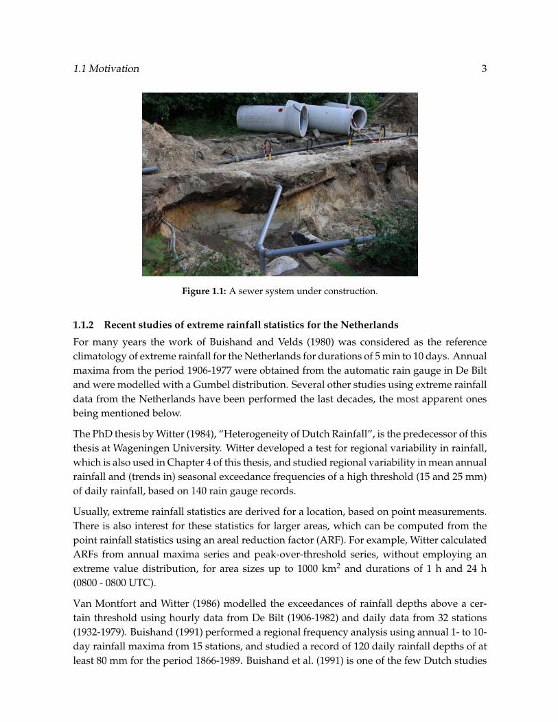
Figure 1.1: A sewer system under construction.
1.1.2 Recent studies of extreme rainfall statistics for the Netherlands
For many years the work of Buishand and Velds (1980) was considered as the reference
climatology of extreme rainfall for the Netherlands for durations of 5 min to 10 days. Annual
maxima from the period 1906-1977 were obtained from the automatic rain gauge in De Bilt
and were modelled with a Gumbel distribution. Several other studies using extreme rainfall
data from the Netherlands have been performed the last decades, the most apparent ones
being mentioned below.
The PhD thesis by Witter (1984), “Heterogeneity of Dutch Rainfall”, is the predecessor of this
thesis at Wageningen University. Witter developed a test for regional variability in rainfall,
which is also used in Chapter 4 of this thesis, and studied regional variability in mean annual
rainfall and (trends in) seasonal exceedance frequencies of a high threshold (15 and 25 mm)
of daily rainfall, based on 140 rain gauge records.
Usually, extreme rainfall statistics are derived for a location, based on point measurements.
There is also interest for these statistics for larger areas, which can be computed from the
point rainfall statistics using an areal reduction factor (ARF). For example, Witter calculated
ARFs from annual maxima series and peak-over-threshold series, without employing an
extreme value distribution, for area sizes up to 1000 km2 and durations of 1 h and 24 h
(0800 - 0800 UTC).
Van Montfort and Witter (1986) modelled the exceedances of rainfall depths above a cer-
tain threshold using hourly data from De Bilt (1906-1982) and daily data from 32 stations
(1932-1979). Buishand (1991) performed a regional frequency analysis using annual 1- to 10-
day rainfall maxima from 15 stations, and studied a record of 120 daily rainfall depths of at
least 80 mm for the period 1866-1989. Buishand et al. (1991) is one of the few Dutch studies

4 Chapter 1 — Introduction
devoted to extreme rainfall modelling of subhourly maxima: 15-min annual maxima were
abstracted from 25-year records of three automatic rain gauges. Buishand (1993) derived
rainfall depth-duration-frequency (DDF) curves for durations of 1 to 10 days using daily
rainfall depths from De Bilt for the period 1906-1977. Rainfall DDF curves describe the rain-
fall depth as a function of duration for a given return period. Because of a similar climate,
Belgian studies are also of interest for the Netherlands, such as Delbeke (2000), Willems
(2000) and Gellens (2003). Delbeke (2000) calculated depth-duration-frequency curves using
the Gumbel distribution for durations of 10 min to 7 days based on a 100-year record from
Uccle, Belgium, and several shorter records (18-28 years) in Flanders. Gellens (2003) consid-
ered the whole of Belgium and applied the Generalized Extreme Value (GEV) distribution.
Smits et al. (2004) derived a climatology for the Netherlands, a new reference, using the time
series of the automatic rain gauge in De Bilt for the period 1906-2003. They applied a GEV
distribution and a peak-over-threshold method to model rainfall maxima for durations of
4 h to 9 days and briefly investigated whether the statistics for the Bilt are representative of
the rest of the country. In addition to this report, Buishand and Wijngaard (2007) performed
a new analysis of the 5-min to 120-min annual maxima from De Bilt from 1906-1990 using the
GEV distribution. Based on a recommendation from Smits et al. (2004) an extensive regional
analysis was undertaken in the framework of the project “Van neerslag tot schade”: Buis-
hand et al. (2009) studied regional differences in extreme rainfall for durations of 1 to 9 days
using 55-year records of daily rainfall depths obtained from 141 manual rain gauges, most of
them from the same locations as used in Witter (1984). They found that the rainfall statistics
from De Bilt are representative of a large part of the country, however, for several parts the
extreme value statistics from De Bilt should be multiplied with a correction factor varying
from 0.93 to 1.14. Some other recommendations by Smits et al. (2004) are combining records
from several stations to reduce the uncertainty in estimated extreme rainfall statistics, which
was followed in Buishand et al. (2009), and the calculation of extreme areal rainfall statistics,
which is particularly important for water authorities. A final recommendation concerns the
regional variability of extreme subdaily rainfall, which remains a topic that has hardly been
studied.
1.1.3 Potential of weather radar
Precipitation is measured operationally using primarily rain gauges, ground-based weather
radars and satellites. Quantitative precipitation estimation (QPE) from satellites is con-
sidered to be less accurate than from rain gauges and radars, but is particularly valuable
over oceans and remote areas, where few ground-based (remote sensing) measurements are
available. Weather radars have become an important tool for real-time QPE over large areas
and are, for instance, used in water management and nowcasting of precipitation. Current
operational weather radars have a spatial resolution of typically 1 km in the horizontal and a
temporal resolution of 5 min. Figure 1.2 shows the KNMI radar tower in De Bilt, the Nether-
lands (left). KNMI radar rainfall products are extensively used by the hydrological commu-

1.1 Motivation 5
Figure 1.2: The radar tower in De Bilt, the Netherlands (left), view from the radar in De Bilt in the
direction of a major building which partly blocks the lowest radar beam (middle), the
best of two worlds (right): combine the rain gauge (in front) and the weather radar (back-
ground). The radome protects the antenna of the radar system.
nity, especially water authorities, and there is even a tendency to start using these products
for urban water management. This is the result of the improved quality of radar rainfall
products and new commercial hydrological software. A development in the Netherlands is
the KNMI warning system for water authorities which uses the precipitation history, and
nowcasting of precipitation from weather radar and a numerical weather prediction model
to forecast rainfall, and is operational since 2003 (Kok et al., 2009). Taking into account the
local discharge and storage capacity, automatic warnings are issued if chosen thresholds of
rainfall depths are exceeded with a certain probability. This system is used by about half of
the water authorities in the Netherlands. Radar could also be potentially useful for deriving
extreme rainfall statistics, particularly for short durations and for different areas.
The number of radars has grown steadily over the years resulting in an almost complete
coverage of, among others, the United States and Europe. Nowadays, the general public
can freely access real-time radar images of rainfall intensities on the Internet, the most well-
known radar product. Another product is the radar echotop, based on reflectivity data from
typically 15 scan elevations providing an indication of the maximum height of showers,
which is important for aviation meteorology. In addition to QPE, weather radars of the
Doppler type can also be used to obtain wind profiles or, by combining output of more
radars, horizontal dual-Doppler wind fields if it is raining. A new development is to monitor
bird migration using operational weather radars, currently investigated in the framework of
the project Flysafe of the European Space Agency (Dekker et al., 2008). This is of importance

6 Chapter 1 — Introduction
Figure 1.3: This figure shows the many errors which may hamper quantitative precipitation estima-
tion using weather radar. Reproduced by permission of Markus Peura (Finnish Meteoro-
logical Institute).
for the biological community and for aviation, in order to prevent bird strikes.
Radar can be useful to derive subdaily extreme rainfall depths. Several studies present sub-
daily extreme rainfall statistics using rain gauges, for instance, Koutsoyiannis et al. (1998),
Alila (1999) and Madsen et al. (2002). However, the description of regional variability of ex-
treme rainfall statistics and the study of extreme rainfall over an area have often been ham-
pered by the low density of rain gauge networks and the lack of digitized time series. With
the long time series that become available, radar holds a promise to bridge this gap. How-
ever, as discussed more extensively in Chapter 3, QPE from weather radar can be hampered
by a number of errors. See Figure 1.3 for an overview. One of the errors is beam-blockage:
Figure 1.2 (middle) shows a photograph, which was taken from the radar, of a building lo-
cated 1.9 km from the radar site in De Bilt, which blocks part of the lowest radar beam over
an azimuth of 4◦. The influence at longe range from the radar of this specific building on
the monthly accumulated rainfall depth can be seen in the area indicated by the white box
in Figure 3.3 (a, page 56).
Radar measures precipitation indirectly, using several assumptions, and at larger altitudes
above the earth’s surface, whereas for most applications rainfall at the earth’s surface is of
interest. Therefore, it is necessary to adjust radar rainfall depths before these can be used to
derive a rainfall climatology. Volumetric (3-D) radar data can be employed to obtain better
precipitation estimates. Unfortunately, long time series (10 years or so) of volumetric radar
data will in general not be available up to now, at least not for the Netherlands.

1.1 Motivation 7
Figure 1.4: The manual rain gauge (left) and the automatic rain gauge (right) part of KNMI’s rain
gauge networks.
The alternative for obtaining high-quality radar rainfall depths is to employ rain gauge data
to adjust 2-D radar data, an approach also followed in this thesis. Rain gauge data are as-
sumed to provide accurate point measurements of rainfall, while weather radars give semi-
quantitative precipitation estimates. In contrast, radars are capable of revealing the spatial
structure of rainfall in detail, whereas this can usually not be obtained from rain gauges. The
best of two worlds is to combine weather radar with rain gauge data (Figure 1.2, right). For
that purpose, both KNMI rain gauge networks were utilized: an automatic network with
1-h rainfall depths for each clock-hour (≈ 1 station per 1000 km2) and a manual network
with 24-h 0800-0800 UTC rainfall depths (≈ 1 station per 100 km 2). Figure 1.4 shows the
manual rain gauge (left) and the automatic rain gauge (right) which is used at most auto-
matic weather stations. The automatic rain gauge is surrounded by a wall with a height of
0.40 m to avoid undercatch due to turbulence.
1.1.4 Research questions
In the overview of recent studies in Section 1.1.2, several recommendations are given for
further research, which provided a motivation for the current project. Apart from these rec-
ommendations, another important aspect is that uncertainties in extreme rainfall events are
often disregarded and are not incorporated in the design of hydraulic structures leading to
an increased risk. This shows the importance of estimating the uncertainty in extreme rain-
fall statistics. This leads to the following research question:
• How to quantify the uncertainty in rainfall depth-duration-frequency (DDF) curves?

8 Chapter 1 — Introduction
Section 1.1.3 shows the potential of QPE with radar. Given the large number of possible
errors in QPE with radar, one might wonder whether adjustment procedures succeed in re-
moving these errors for extreme rainfall events sufficiently. In addition, an 11-year record
could be too short to obtain reliable extreme rainfall depths from an extreme value model,
resulting in the next research question:
• How reliable are the rainfall depths for given return periods based on weather radar?
The high spatial resolution of radar data and the availability of 12 long rain gauge records
of subdaily rainfall provide new opportunities to study regional variation in extreme rain-
fall in the Netherlands. Often, the extreme rainfall data which are used by the hydrological
community, are from the automatic rain gauge in De Bilt, in the middle of the country. This
is not appropriate in the case of regional variability in extreme rainfall. Therefore, attention
is given to the research question:
• Are regional differences in extreme rainfall significant for durations of 15 min to 24 h?
Quite often the actual interest is not in extreme point rainfall statistics but in extreme areal
rainfall statistics. Generally, dense rain gauge networks are not available. Because of the
large number of observations in space, weather radar holds a promise in deriving DDF
curves for larger area sizes. This gives rise to the research question:
• What is the value of weather radar to obtain areal DDF curves?
1.2 Quantitative precipitation estimation from weather radar
Radar is frequently used for remote sensing of the atmosphere. Radars developed during
World War II to detect enemy aircraft also revealed precipitation echoes, which were con-
sidered as noise. Since then, radars have been developed which were specifically designed
to detect precipitation. In Chapter 3 a description is given of quantitative precipitation es-
timation from weather radar including possible (sources of) errors. In this section the mea-
surement principle of a typical operational weather radar is discussed in more detail.
1.2.1 Pulses, echo powers and sampling
The KNMI weather radars transmit electromagnetic radiation as pulses with a duration τ of
0.8 or 2 µs and a repetition frequency between 250 Hz and 1200 Hz. These high-frequency
signals (5.6 GHz) are generated by a magnetron transmitter and transferred to the antenna
by means of a waveguide, which is a hollow, rectangular metal tube matched to wavelength
λ shown in Figure 1.5 (left). The antenna feed of the waveguide is located at the focal point of
a circular parabolic reflector with a diameter of 4.2 m, see Figures 1.5 (right) and 1.6. Thus,

1.2 Quantitative precipitation estimation from weather radar 9
Figure 1.5: Transmitter cabinet, receiver cabinet and waveguide (left), and the circular parabolic re-
flector of the KNMI weather radar in De Bilt.
the pulse transmitted by the antenna feed is reflected into the atmosphere by the circular
parabolic reflector. Since the reflector is directional, most power is captured in the central
portion of the beam, the main lobe, in all directions perpendicular to the electromagnetic
wave, called the half-power beamwidth φ (◦):
φ =70λ
d, (1.1)
where d is the diameter (m) of the circular parabolic reflector. For the KNMI radar this is
approximately 1◦. A small part of the power is contained in the sidelobes, which occur in
every direction. The main lobe has approximately a Gaussian beam pattern. The gain is
defined as:
g =p1
p2, (1.2)
with p1 the power on the axis of the radar antenna and p2 the power on the same location
without an antenna. The KNMI antennas have a gain of approximately 2.0 · 104 (43 dB).
Part of the radiation is backscattered by hydrometeors, such as rain droplets, snow flakes
and ice crystals. The receiver of the radar system is capable of measuring the backscattered
echoes. Because the reflector is directional, the position of targets can be computed from the
range, the beam elevation with respect to the earth’s surface and the azimuth, which is the
direction of the radar antenna in terms of the 360◦ compass (Rinehart, 2004). The range of
a target r (km) with respect to the radar can be calculated from the time delay of the echo
using:
r =ct
2, (1.3)
where c is the speed of light (km s−1) and t (s) is the time delay between transmission and
reception of a pulse.

10 Chapter 1 — Introduction
Figure 1.6: The circular parabolic reflector with antenna feed, together named antenna, of the KNMI
weather radar in De Bilt.
The quality of the observations clearly deteriorates at long ranges and is of limited value be-
yond ranges of approximately 200 km. This is caused by overshooting of precipitation, due
to the larger height of the radar beam above the earth’s surface. Moreover, in the derivation
of the radar equation it is assumed that a radar sample volume is homogeneously filled with
randomly scattered precipitation particles, whereas partial beam filling may occur: since the
measurement volume increases with range, the same storm will occupy a relatively small
part of the measurement volume at long ranges leading to a reduction in the received echo
powers (Rinehart, 2004).
The radar measures echo powers in 360 azimuth sectors of 1◦, each of them containing range
gates with a size of 125 m. Note that the radar reflectivity factor (see Section 1.2.2) from a
single pulse assigned to a certain range gate is a measurement over a distance of 300 m
(for τ = 2 µs) in the direction of the radar resulting in a spatially smoothed measurement.
The signal processor converts the echo powers to radar reflectivity factors using the radar
equation. For the lowest elevation angle of 0.3◦, approximately 14 pulses are transmitted for
each 1◦-azimuth sector from which the corresponding radar reflectivity factors are averaged
over each range gate. Since the beam also covers adjacent azimuth sectors, the average
radar reflectivity factor of a range gate is influenced somewhat by hydrometeors in those
surrounding sectors.
Subsequently, the radar reflectivity factors from the first 8 adjacent range gates are averaged.
This is repeated for the next 8 adjacent range gates, and so on. This results in a table with
elements of radar reflectivity factors as a function of azimuth and range. The advantage of
averaging reflectivity factors is that each element covering 1◦ × 1 km is based on 112 pulses
(for an elevation angle of 0.3◦), so that they become more accurate. These elements can be

1.2 Quantitative precipitation estimation from weather radar 11
projected on a polar stereographic grid with pixels having a spatial resolution of 2.4 × 2.4
km2 (this thesis). The spatial resolution has been increased to 1 × 1 km2 from January 2008.
1.2.2 The radar equation
In this section the main steps in deriving the radar equation are described. This equation
is utilized to convert echo powers measured by the receiver of the radar system to radar
reflectivity factors. For an isotropic antenna, the same amount of power is transmitted in all
directions. The power is distributed over the surface of a sphere, leading to a power per unit
area, a power density S (W m−2) of:
S =pt
4πr2, (1.4)
with pt the transmitted power (W) and r the range from the radar (m). For the KNMI
weather radars pt is approximately 270 kW. Since a weather radar has a directional antenna,
Eq. 1.4 has to be multiplied by the gain from Eq. 1.2. A target with cross section σ (m2) along
the beam axis intercepts a power pσ (W):
pσ =ptgσ
4πr2, (1.5)
where σ is not necessarily equal to the physical size of the target.
Hydrometeors have an approximately spherical shape and their diameter D is usually small
with respect to the wavelength of the radar pulse, i.e., D/λ < 0.1, with λ being approxi-
mately 0.053 m for C-band radars. Because of this, the Rayleigh scattering approximation
holds, so that the backscattering cross section of an individual target, σi (m2), is given by:
σi =π5|K|2D6
i
λ4, (1.6)
where |K|2 is a coefficient related to the dielectric constant of the hydrometeor (0.93 for
liquid water and 0.197 for ice). Note that cloud particles can only be detected by operational
weather radars at very short ranges.
Because a backscattering cross section is used, targets are assumed to reflect the power
isotropically and only part of this radiation, pr, is measured by the receiver of the radar
system:
pr =pσ Ae
4πr2=
ptgσi Ae
16π2r4, (1.7)
where Ae is the effective area of the antenna, which is given by:
Ae =gλ2
4π. (1.8)
This leads to the following radar equation for the averaged received power from a point
target at the centre of a radar beam (Rinehart, 2004).
pr =ptg
2λ2σi
64π3r4. (1.9)

12 Chapter 1 — Introduction
The volume a radar samples, V, may contain many rain droplets or ice particles, which all
have an individual backscattering cross section. The radar reflectivity η is given by:
η = ∑vol
σi =σt
V, (1.10)
where σt is the total reflectivity and vol represents a unit volume of 1 m3. Replacing σi in
Eq. 1.9 with σt and substituting Eq. 1.6 gives:
pr =ptg
2π2|K|2Vη
64λ2r4, (1.11)
where V is the volume of the radar sample. Probert-Jones (1962) developed an expression
for V for circular parabolic reflectors, which takes into account the approximate Gaussian
shape of the beam pattern:
V =πr2θφcτ
16 log 2, (1.12)
with θ and φ the horizontal and vertical beamwidths (radians), which are usually equal.
This replaced an empirical factor in the radar equation, which was needed to obtain bet-
ter precipitation estimates (Marshall et al., 1955). Probert-Jones realized that this unknown
factor was due to the power distribution in the main lobe which was not taken into account.
Since the diameters of the individual rain droplets are not known, a radar reflectivity factor
Z is defined, which is independent of radar type and wavelength, and therefore a property
of the atmosphere:
Z = ∑vol
D6. (1.13)
Eqs. 1.11 and 1.12 contain a number of properties of the radar: pt, g, θ, φ and λ and a number
of constants, which are combined in the so-called radar constant C. Now, the radar reflec-
tivity factor Z (mm6 m−3) can be calculated with the following form of the radar equation:
Z = Cprr2. (1.14)
Because of the large range of measured values of Z, this quantity is usually expressed on a
logarithmic scale:
ZdB ≡ 10 ×10 log
[Z
1 mm6/m3
](1.15)
where ZdB is the logarithmic radar reflectivity factor (dBZ). This can also be done for the
power pr leading to PrdB. Then, the following expression is obtained:
ZdB = CdB + PrdB + 20 ×10 log r + 2ar, (1.16)
where an extra term 2ar is added, which represents losses due to atmospheric attenuation
between antenna and target, a being the gaseous attenuation coefficient. Some other losses

1.2 Quantitative precipitation estimation from weather radar 13
are usually taken into account in the radar constant, such as waveguide, radome and re-
ceiver losses. Attenuation losses due to high rainfall intensities or a wet radome are not
considered and are difficult to account for in an operational setting for single-polarization
radars. In the derivation of the radar equation many assumptions have been made, which
have been described more comprehensively in Collier (1989). The derivation of the radar
equation was based on Raghavan (2003) and Rinehart (2004).
1.2.3 From radar reflectivity factor to rainfall intensity
In this section particular attention is given to the Z-R relation, which is used to convert radar
reflectivity factors Z to rainfall intensities R. Using raindrop measurements at the ground,
Marshall and Palmer (1948) found that the raindrop size distribution can be approximated
by an exponential distribution:
N(D) = N0e−ΛD, (1.17)
with D the drop size diameter (mm) and N(D)dD the mean number of raindrops with a
diameter between D and D + dD in a unit volume of air, and N0 = 8 × 103 mm−1 m−3.
The raindrop size distribution is determined by coalescence and breakup, see, for instance,
Doviak and Zrnic (1993). The coefficient Λ (mm−1) was found to depend on the rainfall
intensity R (mm h−1):
Λ = 41R−0.21. (1.18)
Under the assumption of Rayleigh scattering, Z can be expressed as the sixth moment of the
drop size distribution N(D):
Z =∫ ∞
0N(D) · D6 dD, (1.19)
which is a continuous approximation of Eq. 1.13. Using the gamma function,
Γ(x) =∫ ∞
0tx−1e−tdt, (1.20)
and the Marshall-Palmer drop size distribution (Eq. 1.17), a general expression can be de-
rived for the moments of the drop size distribution M(x):
M(x) =∫ ∞
0N0e−ΛD · Dx dD =
N0Γ(x + 1)
Λx+1. (1.21)
For instance, Z can now be written as:
Z = M(6) =N0Γ(7)
Λ7=
720N0
Λ7. (1.22)
By substituting Eq. 1.18 into Eq. 1.22 a Z-R relationship is obtained (Marshall and Palmer,
1948):
Z = 296R1.47. (1.23)
Another way to obtain a Z-R relationship is to develop an expression for the rain rate R. The
volume of water in one m3 of air is given by:∫ ∞
0
1
6πD310−9N(D)dD. (1.24)

14 Chapter 1 — Introduction
The rate of precipation (a flux) is obtained by dividing Eq. 1.24 by an area of one m2 and
multiplying with the terminal fall speed of drops v(D) (m s−1):
R =∫ ∞
0103 · 3600 ·
1
6πD310−9N(D)v(D)dD, (1.25)
with
v(D) ≃ αDβ. (1.26)
Atlas and Ulbrich (1977) found values of 3.778 and 0.67 for respectively the coefficients α
and β. Using Eq. 1.21, the total rate of precipitation R (mm h−1) can now be expressed as:
R = 6 · 10−4πα
∫ ∞
0N(D)D3+βdD ≡ 6 · 10−4παM(3 + β) =
6 · 10−4παN0Γ(4 + β)
Λ4+β, (1.27)
which is an expression of R as a moment of the drop size distribution N(D). Eliminating Λ
using Eqs. 1.22 and 1.27 results in:
Z = 237R1.50. (1.28)
This shows inconsistency in the Z-R relations (compare to Eq. 1.23), which has been inves-
tigated in detail by Uijlenhoet and Stricker (1999), who also developed a consistent rainfall
parameterization.
The most widely used Z-R relationship, which is also used for the KNMI radars, is given by:
Z = 200R1.6, (1.29)
and was found by Marshall et al. (1955) from raindrop records at the ground. Eq. 1.13 was
used to calculate Z. This relationship is representative for average conditions. However,
these values may differ considerably depending on rainfall type, and will lead to errors in
the case of snowfall.
1.3 Outline
This thesis is organized as follows. Chapter 2 starts with the calculation of extreme rainfall
statistics for durations of 1 to 24 h using records from 12 automatic gauges from the Nether-
lands. Most of these records have not been employed before for this specific application.
The regional variability in extreme rainfall is studied. A methodology is presented to de-
rive the regularly used rainfall depth-duration-frequency (DDF) curves, which describe the
rainfall depth as a function of duration for a given return period. Attention is given to the
estimation of uncertainties in these curves.
The thesis proceeds with the derivation and verification of a 10-year data set of 1- to 24-
h radar rainfall depths in Chapter 3 covering the land surface of the Netherlands. Using
the climatological data set of rainfall depths from Chapter 3, an extreme value analysis is
performed in Chapter 4 for durations of 15 min to 24 h. Rainfall DDF curves are derived
and it is studied whether regional variability in extreme rainfall is significant. In Chapter 5

1.3 Outline 15
areal reduction factors and areal rainfall DDF curves are obtained from weather radar for
areas ranging from a radar pixel to the size of a catchment. The thesis ends with conclusions
and an outlook.

16 Chapter 1 — Introduction

Chapter 2
Rainfall depth-duration-frequency curves
and their uncertainties1
Abstract
Rainfall depth-duration-frequency (DDF) curves describe rainfall depth as a function of duration for
given return periods and are important for the design of hydraulic structures. This chapter focuses
on the effects of dependence between the maximum rainfalls for different durations on the estima-
tion of DDF curves and the modelling of uncertainty of these curves. For this purpose the hourly
rainfall depths from 12 stations in the Netherlands are analysed. The records of these stations are
concatenated to one station-year record, since no geographical variation in extreme rainfall statistics
could be found and the spatial dependence between the maximum rainfalls appears to be small. A
Generalized Extreme Value (GEV) distribution is fitted to the 514 annual rainfall maxima from the
station-year record for durations of 1, 2, 4, 8, 12 and 24 h. Subsequently, the estimated GEV parame-
ters are modelled as a function of duration to construct DDF curves, using the method of generalized
least squares to account for the correlation between GEV parameters for different durations. A boot-
strap estimate of the covariance matrix of the estimated GEV parameters is used in the generalized
least squares procedure. It turns out that the shape parameter of the GEV distribution does not vary
with duration. The bootstrap is also used to obtain 95%-confidence bands of the DDF curves. The
bootstrap distribution of the estimated quantiles can be described by a lognormal distribution. The
parameter σ of this distribution (standard deviation of the underlying normal distribution) is mod-
elled as a function of duration and return period.
1Journal of Hydrology, 2008, 348, pp 124-134 by Aart Overeem, Adri Buishand and Iwan Holleman.
17

18 Chapter 2 — Rainfall depth-duration-frequency curves and their uncertainties
2.1 Introduction
Statistics of extreme rainfall are important to society for (i) design purposes in water man-
agement - such as the construction of sewerage systems, determination of the required dis-
charge capacity of channels and capacity of pumping stations - in order to prevent flooding,
thereby reducing the loss of life and property, and pollution of surface waters; (ii) insurance
of water damage and evaluation of hazardous weather, e.g. of interest for liability; (iii) ad-
vice to the general public. See e.g. Stewart et al. (1999) and Koutsoyiannis and Baloutsos
(2000) for more on this subject. Accordingly, reliable calculation of probabilities of extreme
rainfall with their uncertainties is of concern. Uncertainties should be taken into account,
otherwise risks can be underestimated. Frequently statistics of extreme rainfall are con-
tained in rainfall depth-duration-frequency (DDF) curves, which describe rainfall depth as
a function of duration for given return periods or probabilities of exceedance.
In particular for short durations, rainfall intensity has often been considered rather than
rainfall depth, leading to intensity-duration-frequency (IDF) curves. The method of deriva-
tion of the two types of curves is, however, identical. Koutsoyiannis et al. (1998) present a
mathematical framework for studying IDF relationships, which also applies to DDF curves.
The first step in the construction of DDF curves is fitting some theoretical distribution to the
extreme rainfall amounts for a number of fixed durations. A logical step to proceed then is
to describe the change of the parameters of the distribution with duration by a functional
relation. From the fitted relationships the rainfall depths for any duration and return period
can be derived. A problem in this approach is that the estimated parameters for different
durations are correlated. Standard regression techniques may then not be appropriate to
estimate the unknown coefficients in the relationships that determine the DDF curves and
the uncertainty of these relationships. Buishand (1993) studied the influence of correlation
on the determination of DDF curves for De Bilt (The Netherlands) using the annual maxi-
mum amounts for durations between 1 and 10 days. A Gumbel distribution was fitted to
these annual maxima. It was demonstrated that ignorance of the correlation between the
estimated Gumbel parameters results in an underestimation of the standard deviation of
the estimated quantiles from the DDF curves. Confidence bands of these curves and other
measures of uncertainty should therefore take this correlation into account.
Though frequently used, the Gumbel distribution may underestimate quantiles for long re-
turn periods, see e.g. Buishand (1991), Koutsoyiannis and Baloutsos (2000) and Koutsoyian-
nis (2004). A widely-used alternative is the Generalized Extreme Value (GEV) distribution,
which allows for a better description of the upper tail of the distribution, due to an addi-
tional parameter. Large samples are needed to estimate this shape parameter accurately or
data from several sites in a region should be pooled assuming that the shape of the distribu-
tion does not change over the region.

2.2 Rainfall data 19
This chapter deals with the construction of DDF curves for short durations (1-24 h) in the
Netherlands using the GEV distribution. The GEV distribution is fitted to the annual max-
ima of a station-year record of 514 years based on the hourly data of 12 stations. Subse-
quently, using the method of generalized least squares a relation of the GEV parameters as
a function of duration is estimated. The correlations between the parameter estimates for
different durations are taken into account.
The bootstrap is used both for the estimation of correlation between estimated GEV param-
eters and for the confidence bands of the DDF curves. The latter shows similarities with the
resampling technique presented by Burn (2003) to calculate confidence intervals for flood
quantiles. Innovative aspect of this chapter is that the uncertainty in rainfall DDF curves is
described with a lognormal probability distribution.
This chapter is organized as follows. First, the data are described. Next, the construction of
the station-year record is justified. Subsequently, the GEV fits to the annual maxima of this
record and the modelling of the change of the GEV parameters with duration are addressed.
This is followed by a description of the construction of DDF curves and their uncertainties.
The chapter closes with a discussion and conclusions.
2.2 Rainfall data
2.2.1 Rain gauge networks
KNMI maintains two independent rain gauge networks: an automatic network of approx-
imately 35 gauges (≈ 1 station per 1000 km2) and a manual network of approximately 325
gauges (≈ 1 station per 100 km2). Originally the automatic network was operated using
mechanical pluviographs. These have been replaced by electronic rain gauges from the end
Table 2.1: Selected stations, their record length, latitude, longitude and elevation.
Station name Record length (years) Latitude (N) Longitude (E) Elevation (m)
Beek 48 50.92◦ 5.78◦ 114
De Bilt 99 52.10◦ 5.18◦ 2
De Kooy 49 52.92◦ 4.79◦ 0
Eelde 49 53.12◦ 6.59◦ 4
Gilze-Rijen 29 51.57◦ 4.93◦ 11
Leeuwarden 30 53.22◦ 5.75◦ 0
Schiphol 35 52.30◦ 4.77◦ -4
Twente 31 52.27◦ 6.90◦ 35
Valkenburg 32 52.18◦ 4.42◦ 0
Vlissingen 49 51.44◦ 3.60◦ 8
Volkel 31 51.66◦ 5.71◦ 20
Zestienhoven 32 51.95◦ 4.44◦ -5

20 Chapter 2 — Rainfall depth-duration-frequency curves and their uncertainties
0 50
N
Beek
De Bilt
De Kooy
Eelde
Gilze−Rijen
Leeuwarden
Schiphol TwenteValkenburg
Vlissingen
Volkel
Zestienhoven
km
Figure 2.1: Map of the Netherlands with the locations of the 12 stations considered in this chapter.
of the 1970s. The electronic rain gauge measures the precipitation depth using the displace-
ment of a float placed in a reservoir. The 24-h precipitation depth from the manual gauges
is measured at 0800 UTC. Detailed information on the rain gauge networks of KNMI can be
found in KNMI (2000).
To perform a reliable extreme value analysis, only stations with automatic rain gauges were
selected for which at least 29 years of hourly precipitation depth data were available from
the mid 1970s. It is noted that these depths are clock-hour sums. This selection resulted in
a data set with time series from 13 stations distributed over the Netherlands. The 30-year
record of one station was removed, since it was located only 7 km from De Bilt, for which a
much longer record was available.
The locations of the selected stations are shown in Figure 2.1 and are listed in Table 2.1.
The time series, in total 514 station years, all end in 2005. If more than 5 days in a year
were missing, the year was removed from the data set. In total only 3 station years were
removed. For the automatic gauge in De Bilt, the annual 1-h and 2-h rainfall maxima based
on continuous recording, so-called sliding maxima, are available for the period 1906-1990.
The data from the manual network were only used for adjustment of the automatic gauge
observations (see below). Until the mid 1990s all stations were equipped with a collocated
manual gauge. In 2005, the distance between the selected automatic gauges and the nearest
manual gauge ranged from 0.3 to 6.1 km.

2.3 Regional variability in extreme rainfall statistics 21
0 10 20 30 40 50
010
2030
4050
Manual gauge (mm)
Aut
omat
ic g
auge
(m
m)
De Bilt1987
Figure 2.2: Daily precipitation depths (mm) of automatic versus manual gauges for De Bilt during
1987. The straight line is the y = x line.
2.2.2 Adjustment of automatic gauge data
The WMO (1981) Guide to Hydrological Practices states that “it was decided that the stan-
dard nonrecording rain gauge measurements should be the official rainfall readings at the
station, and that a correction factor should be applied to hourly rainfall and maximum in-
tensity data, based on the ratio of the daily total by standard gauge to the total by recording
gauge.” Before 1982 the archived hourly sums from the automatic gauges were adjusted by
default with the daily sums from the collocated manual gauge. From 1982 the annual rain-
fall sums from the manual gauges are on average 5% larger than those from the automatic
gauges. To promote the homogeneity of the data set it was decided to adjust the remaining
56% of automatic gauge data (1982-2005) by the same procedure, so also the data from the
mid 1990s using the readings from the nearest manual gauge.
Figure 2.2 shows a typical scatter plot of the daily precipitation depths from the automatic
and the manual gauges in De Bilt during one year. Evidently the two gauges correspond
rather well and the adjustment factors are generally close to unity. The extreme value anal-
ysis presented in the remainder of this chapter has been carried out using the adjusted data
set. When the same analysis is performed on the (partly) unadjusted data set the differences
are small.
2.3 Regional variability in extreme rainfall statistics
The Netherlands has a temperate climate with mean annual rainfall varying from 768 to
848 mm for the 12 selected stations. This low variation is due to the absence of significant
orography. Most daily (0800-0800 UTC) annual maxima occur in the period May to Decem-

22 Chapter 2 — Rainfall depth-duration-frequency curves and their uncertainties
ber, whereas most annual 1-h maxima occur from May to September, caused by the larger
influence of convective rainfall in summer. In this section regional variability in extreme
rainfall statistics is investigated. First the GEV distribution is introduced. Then the regional
variability of its parameters is studied.
2.3.1 Fitting a GEV distribution
The GEV distribution has been used worldwide to model rainfall maxima, see e.g. Schae-
fer (1990), Alila (1999), Gellens (2002), Fowler and Kilsby (2003) and Koutsoyiannis (2004).
Applications to rainfall maxima in the Netherlands are given by Buishand (1991) and Smits
et al. (2004). The GEV cumulative distribution function F(x) is given by (Jenkinson, 1955):
F(x) = exp{−[1 −κ
α(x − µ)]1/κ} for κ 6= 0, (2.1)
F(x) = exp{− exp[−1
α(x − µ)]} ≡ exp{− exp[−y]} for κ = 0, (2.2)
with µ the location, α the scale and κ the shape parameter of the distribution and y the Gum-
bel reduced variate, y = − ln(− ln F). The GEV distribution combines the three asymptotic
extreme value distributions into a single distribution. The type of extreme value distribu-
tion is determined by κ: EV1 (Gumbel distribution) if κ = 0; EV2 (Frechet type) if κ < 0;
and EV3 (Weibull type) if κ > 0. The Frechet type has a longer upper tail than the Gum-
bel distribution and the Weibull type a shorter tail. Using L-moments diagrams Schaefer
(1990), Alila (1999) and Kysely and Picek (2007) show that the GEV distribution describes
the distribution of the annual maximum rainfall amounts much better than the Pearson type
III distribution and that the GEV distribution is generally also preferable to the generalized
logistic distribution. Besides, the GEV distribution is based on asymptotic theory about the
distribution of maxima.
The quantile function, the inverse of Eqs. (2.1) and (2.2), is given by:
x(T) = µ +α{
1 − [− ln(1 − T−1)]κ}
κ= µ + α
1 − exp(−κy)
κfor κ 6= 0, (2.3)
x(T) = µ − α ln[− ln(1 − T−1)] = µ + αy for κ = 0, (2.4)
where T = 1/(1 − F) is the return period.
Running annual maxima are abstracted for each of the 12 time series from the selected sta-
tions for durations D of 1, 2, 4, 8, 12 and 24 h. Running implies here that the D-hour rainfall
amounts are calculated for each clock-hour of the year. A GEV distribution is fitted to the
annual maxima for each station and duration separately.
Both L-moments (Hosking and Wallis, 1997) and maximum likelihood (Coles, 2001) have
been used frequently to fit the GEV distribution to annual maxima. For small samples the
estimates based on L-moments generally have lower standard deviation than those based

2.3 Regional variability in extreme rainfall statistics 23
on maximum likelihood if −0.2 < κ < 0.2 (Hosking et al., 1985). Use of maximum likeli-
hood with a Bayesian prior distribution for κ (Martins and Stedinger, 2000) or with a penalty
function (Coles and Dixon, 1999) performs equally well, but is computationally more diffi-
cult. Because of this and the fact that 11 stations have a record length shorter than 50 years,
the method of L-moments is chosen.
L-moments are based on linear combinations of the order statistics of the annual maximum
rainfall amounts. First, the probability weighted moments are estimated by:
b0 = n−1n
∑j=1
xj:n, (2.5)
b1 = n−1n
∑j=2
j − 1
n − 1xj:n, (2.6)
b2 = n−1n
∑j=3
(j − 1)(j − 2)
(n − 1)(n − 2)xj:n, (2.7)
where x1:n ≤ x2:n ≤ ... ≤ xn:n is the ordered sample of annual maxima. The sample L-
moments are then obtained as:
ℓ1 = b0, (2.8)
ℓ2 = 2b1 − b0, (2.9)
ℓ3 = 6b2 − 6b1 + b0. (2.10)
The estimate κ of the shape parameter κ follows from:
κ = 7.8590 c + 2.9554 c2, (2.11)
where
c =2
3 + ℓ3/ℓ2−
ln 2
ln 3. (2.12)
The estimates α and µ of α and µ are subsequently obtained as:
α =ℓ2 κ
(1 − 2−κ) Γ(1 + κ), (2.13)
µ = ℓ1 − α1 − Γ(1 + κ)
κ, (2.14)
with Γ(.) the gamma function.
In this chapter γ = α/µ is considered instead of α. The advantage of using γ is that its
correlation with µ and κ is weak. The shape parameter κ is often assumed to be constant
over a region and can then be estimated by combining all station records in that region. For
the index flood method γ is also considered to be constant in a region. This assumption has
often been made in rainfall frequency analysis (Gellens, 2002; Fowler and Kilsby, 2003; Mora
et al., 2005).

24 Chapter 2 — Rainfall depth-duration-frequency curves and their uncertainties
2.3.2 Regional variability in GEV parameters
In this section the equality of GEV parameters is tested. The tests below assume that spatial
dependence of the annual maxima can be neglected. Figure 2.3, which is representative
of all six durations, shows that the cross correlations between the annual maxima of the
12 stations are small. Data for the common period 1977-2005 were used to estimate these
cross correlations. For annual maxima of daily rainfall it is further shown by Buishand
(1984), using data from 140 stations located in the Netherlands, that the degree of association
decreases with event magnitude. There is almost no association between the occurrence of
large values if the interstation distance is larger than 30 km.
Let θi be the value of a GEV parameter (µ, γ or κ) at station i. The equality of the θi’s can be
tested with the statistic:
X2 =12
∑i=1
(θi − θw)2/σ2(θi), (2.15)
with θi the L-moments estimate of θi and θw the weighted average of the θi’s defined as:
θw =12
∑i=1
ni θi/12
∑i=1
ni, (2.16)
where ni is the record length at station i. The variance σ2(θi) in Eq. (2.15) was based on the
asymptotic covariance matrix of the L-moments estimators of the GEV parameters as given
by Hosking et al. (1985). The variance of γ was obtained from the variances and covariance
of α and µ using the delta method (Efron and Tibshirani, 1993; Coles, 2001):
varγ ≈ [varα + γ2varµ − 2γcov(α, µ)]/µ2. (2.17)
The unknown population parameters in the expressions for the variances were replaced by
the weighted average θw of the at-site estimates. X2 was calculated for D = 1, 2, 4, 8, 12 and
24 h. X2 has an asymptotic chi-square distribution under the null hypothesis θ1 = θ2 =
... = θ12 with 11 degrees of freedom, if there is no spatial dependence between the annual
maxima. The asymptotic distribution has been verified in a Monte Carlo experiment with
constant GEV parameters. From Table 2.2 it can be seen that the values of the X2-statistic
vary between 5.12 and 12.64, which is far below the critical value 19.68 for a test at the 5%
level.
For each duration D the θi’s were also regressed on mean annual rainfall using weighted
least squares (weights proportional to ni). Only for the location parameter of the 8- and 12-h
annual maxima, the slope of the regression line was significant at the 5% level (Student’s
t-test, one-sided for µ, two-sided for γ and κ).
Since no geographical variation in the GEV parameters could be found and the spatial de-
pendence between the stations’ annual maxima is small, the time series from the 12 stations
are concatenated to a single record of 514 years according to the station-year method.

2.4 Regional estimation and modelling of GEV parameters 25
0 50 100 200
−1.
0−
0.5
0.0
0.5
1.0
Distance (km)
Cor
rela
tion
1 hr
0 50 100 200
−1.
0−
0.5
0.0
0.5
1.0
Distance (km)C
orre
latio
n
24 hr
Figure 2.3: Cross correlations between the annual maxima of the 12 stations plotted against distance
for durations of 1 (left) and 24 (right) hour.
2.4 Regional estimation and modelling of GEV parameters
2.4.1 Estimated GEV parameters for individual durations
For the time series of 514 years a GEV distribution (Eq. (2.1)) was fitted to the running annual
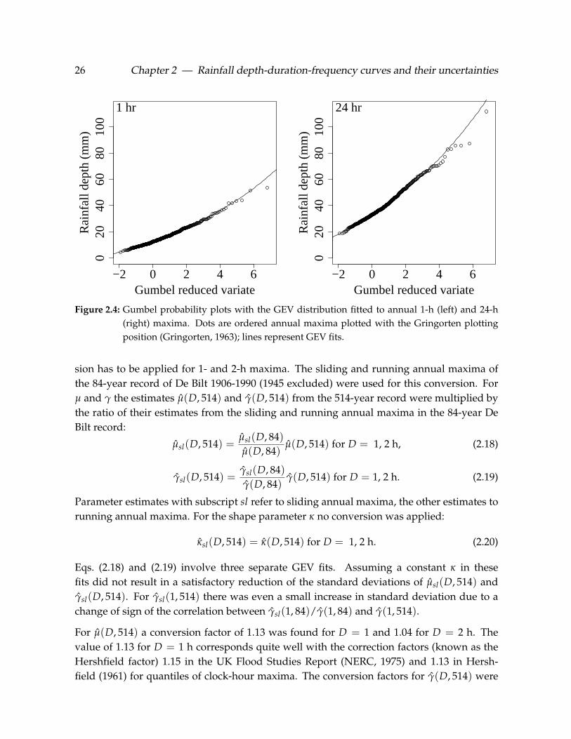
maxima for durations of 1, 2, 4, 8, 12 and 24 h separately. Figure 2.4 shows that the GEV
distribution gives a good fit for the 1-h annual maxima and that there is a weak tendency
to overestimate large quantiles of the 24-h annual maxima. A GEV distribution fitted to 514
annual maxima should give a rather good estimate of large quantiles, particularly because
σ2(κ) is strongly reduced.
Running annual maxima, based on clock-hour rainfall sums, tend to be smaller than sliding
annual maxima, defined as maxima obtained from continuous recording. Because clock-
hour sums are used, the underestimation is small for durations of 4-24 h, however a conver-
Table 2.2: Values of the statistic X2 for testing equality of the GEV parameters µ, γ and κ.
D (h) µ γ κ
1 9.82 10.32 8.82
2 7.45 9.44 10.18
4 5.51 8.98 10.93
8 7.83 7.07 11.61
12 9.35 7.36 9.16
24 12.64 9.01 5.12
26 Chapter 2 — Rainfall depth-duration-frequency curves and their uncertainties
−2 0 2 4 6
020
4060
8010
0
Gumbel reduced variate
Rai
nfal
l dep
th (
mm
)
1 hr
−2 0 2 4 6
020
4060
8010
0
Gumbel reduced variateR
ainf
all d
epth
(m
m)
24 hr
Figure 2.4: Gumbel probability plots with the GEV distribution fitted to annual 1-h (left) and 24-h
(right) maxima. Dots are ordered annual maxima plotted with the Gringorten plotting
position (Gringorten, 1963); lines represent GEV fits.
sion has to be applied for 1- and 2-h maxima. The sliding and running annual maxima of
the 84-year record of De Bilt 1906-1990 (1945 excluded) were used for this conversion. For
µ and γ the estimates µ(D, 514) and γ(D, 514) from the 514-year record were multiplied by
the ratio of their estimates from the sliding and running annual maxima in the 84-year De
Bilt record:
µsl(D, 514) =µsl(D, 84)
µ(D, 84)µ(D, 514) for D = 1, 2 h, (2.18)
γsl(D, 514) =γsl(D, 84)
γ(D, 84)γ(D, 514) for D = 1, 2 h. (2.19)
Parameter estimates with subscript sl refer to sliding annual maxima, the other estimates to
running annual maxima. For the shape parameter κ no conversion was applied:
κsl(D, 514) = κ(D, 514) for D = 1, 2 h. (2.20)
Eqs. (2.18) and (2.19) involve three separate GEV fits. Assuming a constant κ in these
fits did not result in a satisfactory reduction of the standard deviations of µsl(D, 514) and
γsl(D, 514). For γsl(1, 514) there was even a small increase in standard deviation due to a
change of sign of the correlation between γsl(1, 84)/γ(1, 84) and γ(1, 514).
For µ(D, 514) a conversion factor of 1.13 was found for D = 1 and 1.04 for D = 2 h. The
value of 1.13 for D = 1 h corresponds quite well with the correction factors (known as the
Hershfield factor) 1.15 in the UK Flood Studies Report (NERC, 1975) and 1.13 in Hersh-
field (1961) for quantiles of clock-hour maxima. The conversion factors for γ(D, 514) were

2.4 Regional estimation and modelling of GEV parameters 27
0.94 and 0.98 for D = 1 and D = 2 h, respectively. This implies that the correction factor
for quantiles decreases with increasing return period. A disadvantage of the conversion of
γ(D, 514) is that it leads to a considerable increase in the standard deviation (see below).
Table 2.3 gives the estimated GEV parameters and their standard deviations. As expected µ
increases with increasing D. The parameter γ increases with decreasing duration. For this
parameter the standard deviation is relatively high for D = 1 and 2 h as a result of the use of a
short record to adjust the estimate from the 514-year record. There seems to be no systematic
variation of κ with D. This is in line with results of Gellens (2003) for Belgium. The values of
κ deviate 3.5 to 4 times their standard deviation from 0, so the Gumbel distribution would
not be appropriate in modelling the annual rainfall maxima. Negative values of κ have
been found in many other studies for D ≤ 24 h. E.g. Koutsoyiannis (2004) observed that
κ = −0.15 for daily annual maximum rainfall in different climatic zones of the USA, the UK
and the Mediterranean.
In contrast to the use of asymptotic expressions as in Section 2.3.2, the standard deviations
in Table 2.3 were based on the bootstrap. In the bootstrap method new samples (bootstrap
samples) are generated by sampling with replacement from the original sample (Diaconis
and Efron, 1983; Efron and Tibshirani, 1993). The standard deviations in Table 2.3 were
derived from 104 bootstrap samples of 514 years. The algorithm is described in Appendix
A. An advantage of the bootstrap is that it also applies to the estimated GEV parameters for
sliding maxima in Eqs. (2.18) and (2.19). Zucchini and Adamson (1989) were the first who
used the bootstrap to determine the uncertainty of design storms.
2.4.2 Correlations of estimated GEV parameters
The bootstrap also provides for each GEV parameter the correlation coefficients between
the estimates for different durations, which are needed for the assessment of the change of
the parameter with duration. Table 2.4 shows correlation matrices of µ, γ, and κ based on
the same 104 bootstrap samples as in Section 2.4.1. Each correlation matrix consists of the
correlations between the parameter estimates for different durations. These correlations are
due to the dependence between the annual rainfall maxima for different durations. As a
Table 2.3: Estimated GEV parameters for D = 1 (sl), 2 (sl), 4, 8, 12 and 24 h. Standard deviations are
estimated with the bootstrap and given between brackets.
D (h) µ (mm) γ κ
1 14.04 (0.34) 0.343 (0.019) -0.127 (0.033)
2 16.79 (0.31) 0.325 (0.016) -0.112 (0.032)
4 20.08 (0.30) 0.300 (0.011) -0.102 (0.029)
8 24.27 (0.33) 0.271 (0.010) -0.132 (0.033)
12 27.33 (0.36) 0.268 (0.010) -0.121 (0.033)
24 33.08 (0.43) 0.253 (0.010) -0.117 (0.030)

28 Chapter 2 — Rainfall depth-duration-frequency curves and their uncertainties
result correlations between neighbouring durations are quite large. Correlation coefficients
for κ and γ are in general lower than for µ. Table 2.4 also provides the correlations between
the estimates of different GEV parameters for the same duration and shows that especially
corr(µ, γ) and corr(κ, γ) are rather small.
2.4.3 GEV parameters as a function of duration
Relations of GEV parameters as a function of duration D (hour) are used to construct rainfall
DDF curves. In Figure 2.5 GEV parameters are plotted against D for 1, 2, 4, 8, 12 and 24 h.
For D = 1, 2 h GEV parameters are calculated with Eqs. (2.18)-(2.20). It is shown that γ and
the logarithm of µ have a linear relationship with the logarithm of D for D = 1-24 h. There
appears to be no systematic variation of κ with duration.
Figure 2.5 suggests the following regression model for the GEV parameters:
θ = Xβ + e, (2.21)
with θ the vector containing the estimated values of the GEV parameter θ (or its logarithm)
for the six durations D1, .., D6,
Table 2.4: Correlation matrices of µ, γ and κ for D-hour annual maximum rainfall depths and cor-
relations between the estimates of different GEV parameters for the same duration, both
estimated with the bootstrap.
µ γ
D (h) 1 2 4 8 12 24 D (h) 1 2 4 8 12 24
1 1.00 1 1.00
2 0.52 1.00 2 0.49 1.00
4 0.47 0.79 1.00 4 0.39 0.62 1.00
8 0.36 0.62 0.85 1.00 8 0.33 0.41 0.77 1.00
12 0.30 0.52 0.72 0.91 1.00 12 0.22 0.35 0.63 0.86 1.00
24 0.20 0.40 0.58 0.72 0.84 1.00 24 0.15 0.23 0.46 0.56 0.70 1.00
κ
D (h) 1 2 4 8 12 24 D (h) µ, κ µ, γ κ, γ
1 1.00 1 0.22 -0.12 0.07
2 0.73 1.00 2 0.28 0.08 0.13
4 0.49 0.75 1.00 4 0.36 0.18 0.27
8 0.26 0.35 0.61 1.00 8 0.32 0.20 0.23
12 0.21 0.25 0.46 0.88 1.00 12 0.27 0.13 0.16
24 0.08 0.09 0.25 0.62 0.76 1.00 24 0.38 0.31 0.34

2.4 Regional estimation and modelling of GEV parameters 29
1520
2530
D((hr))
µµ((m
m))
1 2 4 8 12 24
0.26
0.28
0.30
0.32
0.34
D((hr))γγ
1 2 4 8 12 24
−0.
130
−0.
120
−0.
110
D((hr))
κκ
1 2 4 8 12 24
Figure 2.5: GEV parameters plotted against duration D. The solid lines represent the generalized
least squares fits to the estimated GEV parameters.
X =
1 ln D1
. .
1 ln D6
,
β =
(a
b
),
and e a vector of random disturbances. The components of e are correlated because of the
correlation between the estimated GEV parameters for different durations. To account for

30 Chapter 2 — Rainfall depth-duration-frequency curves and their uncertainties
this correlation, the method of generalized least squares was chosen to estimate the regres-
sion coefficients a and b. The generalized least squares estimate βGLS of β is given by:
βGLS = (XTC−1X)−1XTC−1θ =
(a
b
), (2.22)
with C the covariance matrix of θ. For γ and κ the estimated correlation coefficients are
given in Table 2.4; for ln µ the estimated correlation coefficients are almost the same as those
for µ. Because of the long time series, these correlation estimates are relatively accurate. Ste-
dinger and Tasker (1985) compared generalized least squares regression with ordinary and
weighted least squares in a regional analysis of streamflow statistics. Madsen et al. (2002)
applied generalized least squares in a regional frequency analysis of rainfall to account for
intersite dependence. The covariance matrix of βGLS is given by:
cov(βGLS) = (XTC−1X)−1. (2.23)
This can be compared with the covariance matrix of the ordinary least squares estimate
βOLS:
cov(βOLS) = (XTX)−1XTCX(XTX)−1. (2.24)
The goodness-of-fit can be tested with the statistic:
X2 = (θ− θGLS)TC−1(θ− θGLS), (2.25)
where θGLS = XβGLS. In the case of an adequate fit, X2 is approximately chi-square dis-
tributed with n − p degrees of freedom, with n = 6 the number of durations and p the
number of regression coefficients. Eq. (2.25) generalizes Eq. (2.15) in two directions: it al-
lows for dependence between the estimated GEV parameters, and it allows for the inclusion
of covariates.
Table 2.5 shows the estimated regression coefficients with their standard deviations. For κ
the estimate of the slope b differs no more from zero than 0.46σ(b). This confirms that κ
may be considered to be constant. Re-estimating a yielded κGLS = a = −0.114, which is
given by the solid line in Figure 2.5. For the other two GEV parameters there is a significant
dependence on duration. The values of the X2-statistic in Table 2.5 are well below the critical
values for a test at the 5% level. So there is no evidence of lack-of-fit.
Table 2.5: Results of the regression of GEV parameters.
GEV parameter a σ(a) b σ(b) X2
ln µ 2.629 0.019 0.273 0.006 3.10
γ 0.341 0.015 -0.028 0.005 4.07
κ -0.125 0.032 0.006 0.013 2.38
κ -0.114 0.021 - - 2.60

2.5 Construction of rainfall DDF curves and their uncertainties 31
For σ(κGLS) a value of 0.021 was found, which is considerably smaller than the standard
deviation of the κ’s for the individual durations in Table 2.3. The ordinary least squares esti-
mate of κ is simply the average -0.119 of the six estimates for the individual durations. The
standard deviation of this average, 0.023, is somewhat larger than σ(κGLS). This confirms
the conclusion in Buishand (1993) that the reduction in standard deviation due to the use
of generalized least squares is small in the case of rainfall depth-duration-frequency analy-
sis. The correlation between the estimated GEV parameters may, however, not be ignored if
standard deviations or goodness-of-fit are of interest.
The systematic change of γ with duration implies that the dependence of quantiles on T and
D cannot be separated in a function of D and a function of T, as was done in Koutsoyiannis
et al. (1998). Another consequence is that simple scaling does not apply as observed by
Menabde et al. (1999) for Melbourne (Australia) and Warmbaths (South Africa) and Borga
et al. (2005) for the Trentino province (Italy). Both require that the coefficient of variation is
constant, which is not the case if γ varies with duration.
2.5 Construction of rainfall DDF curves and their uncertainties
2.5.1 Derivation of DDF curves
Now that the GEV parameters are described as a function of D, rainfall DDF curves are
constructed by substituting these relationships into Eq. (2.3), so that the DDF curves are
given by:
x(T) = exp(aµ + bµ ln D) ×
(1 + (aγ + bγ ln D)
{1 − [− ln(1 − T−1)]κGLS
}
κGLS
), (2.26)
where aµ = 2.629, bµ = 0.273, aγ = 0.341, bγ = -0.028 and κGLS = -0.114.
By choosing a return period T, the rainfall depth x (mm) can be plotted as a function of
duration D using Eq. (2.26). In Section 2.4.3 it was noticed that σ(κ) is considerably reduced
if κ is based on the maxima for all six durations. Large quantiles are then more accurately
estimated compared to fitting a GEV distribution only to the maxima for the duration of
interest. Figure 2.6 presents the DDF curves for T = 100 and 1000 years. The curves show a
strong increase of x with D, e.g. for T = 1000 years rainfall depths range from 64 to 120 mm
for D = 1-24 h.
2.5.2 Modelling uncertainty in DDF curves
Uncertainty in DDF curves is usually disregarded, while it should be considered, e.g. in the
design of hydraulic structures. Here the bootstrap was applied to assess this uncertainty.
This method considers only the uncertainty due to the estimation of the GEV parameters,
i.e. sampling errors. For each of the 104 bootstrap samples from Section 2.4.1 the relations be-
tween the GEV parameters and duration were re-estimated using generalized least squares,
so that 104 DDF curves could be constructed. For each DDF curve the rainfall depths were

32 Chapter 2 — Rainfall depth-duration-frequency curves and their uncertainties
050
100
150
D((hr))
Rai
nfal
l dep
th (
mm
)
050
100
150
1000
1 4 8 12 24
050
100
150
050
100
150
100
1 4 8 12 24
Figure 2.6: Rainfall DDF curves (solid lines) and 95%-confidence bands (dashed lines) for return pe-
riods of 100 and 1000 years (indicated on the right axis).
derived for durations between 1 and 24 h in steps of 1 min. Subsequently, for each of these
durations the 104 depths were ranked in increasing order and the 250th and 9750th values
were determined. Next, these values were plotted and formed the 95%-confidence bands.
For return periods of 100 and 1000 years, Figure 2.6 shows the DDF curves and their 95%-
confidence bands. For T = 1000 years the confidence interval ranges from 55-73 mm for
D = 1 h to 106-135 mm for D = 24 h, thus showing a rather large uncertainty, despite the
fact that the DDF curves are based on a 514-year record. For longer T uncertainty increases
substantially.
It is found that the bootstrap distribution of the estimated quantiles can be described by a
lognormal distribution. The parameters ξ and σ of the lognormal distribution, i.e. the mean
and standard deviation of the underlying normal distribution, are modelled as a function
of D and T. The parameter ξ is well described by the natural logarithm of the estimated
quantiles from the DDF curve. Using 104 bootstrap samples for six durations and seven
return periods, namely from every combination of D = 1, 2, 4, 8, 12 and 24 h and T = 10, 20,
50, 100, 200, 500 and 1000 years, the parameter σ is modelled as:
σ = −0.0042 + 0.0103D−1 + 0.0091 ln T. (2.27)
The regression coefficients were estimated with ordinary least squares. Figure 2.7 shows the
DDF curves for T = 100 and 1000 years. The lognormal probability density functions which
describe the uncertainties in these curves are plotted for D = 1 and 12 h.

2.6 Conclusions 33
050
100
150
D((hr))
Rai
nfal
l dep
th (
mm
)
050
100
150
D((hr))
Rai
nfal
l dep
th (
mm
) 1000
050
100
150
D((hr))
Rai
nfal
l dep
th (
mm
)
050
100
150
D((hr))
Rai
nfal
l dep
th (
mm
)100
1 4 8 12 24
Figure 2.7: Rainfall DDF curves (solid lines) for T = 100 and 1000 years and lognormal probability
density functions (dashed lines) which describe the uncertainties in the DDF curves for
D = 1 and 12 h.
2.6 Conclusions
Extreme rainfall in the Netherlands for durations between 1 h and 24 h was studied. Since
regional variability in extreme rainfall statistics could not be found and spatial dependence
between extreme rainfall amounts appeared to be small, a record of 514 annual maxima
was constructed according to the station-year method. GEV parameters of this time series
were estimated with the method of L-moments. Standard deviations and correlations of
estimated GEV parameters were obtained with the bootstrap. To take into account the cor-
relation between estimated GEV parameters for different durations, the generalized least
squares method was used to describe the variation of these parameters as a function of du-
ration. The relations were used to construct rainfall DDF curves. Finally, uncertainties in
DDF curves, due to sampling variability, were quantified with the bootstrap and described
with a lognormal distribution.
It was found that the shape parameter κ of the GEV distribution does not change with du-
ration. For the parameter γ there is a significant increase with decreasing duration. As a
consequence, the coefficient of variation increases with decreasing duration. This implies
that simple scaling does not hold.
A 84-year record of sliding 1- and 2-h annual maxima from De Bilt was used to convert the
estimated GEV parameters from the 514-year hourly station-year record. For the parameter
γ a correction factor < 1 was found which implies that the correction for quantiles depends
on return period. This may be related to the change of γ with duration.

34 Chapter 2 — Rainfall depth-duration-frequency curves and their uncertainties
In the generalized least squares method used in this chapter to fit relationships between GEV
parameters and duration, the fit for one GEV parameter does not affect the fit for the other
two parameters. This may be justified by the fact that the correlation between the estimated
GEV parameters is small. As an alternative, re-estimation of the parameters µ and γ in the
514-year record was explored assuming κ = κGLS. The changes were very small.
Possible inhomogeneities in the rainfall records due to changed measurement methods,
gauge types or locations were not considered. Further, annual maxima were assumed to
be stationary. Smits et al. (2004) found for De Bilt that the trends in the extremes are rela-
tively small.
Usually uncertainties in rainfall DDF curves are disregarded, so that risks can be under-
estimated. An innovative aspect of this chapter is that uncertainty in DDF curves due to
sampling variability is taken into account. Other sources of uncertainty were not consid-
ered, such as measurement errors and uncertainty about the choice of the distribution.
A situation that there is no regional variability in all GEV parameters will seldom be met
in other parts of the world. In addition, there might be spatial correlation between annual
maximum rainfalls. The methods used here can be adapted if regional variability in GEV pa-
rameters is present. Resampling from the N years providing rainfall data, as e.g. in Faulkner
and Jones (1999), rather than resampling from all station-years, should be considered. Some
care is needed in situations where the covariance matrices of the estimated GEV parameters
vary over the region of interest.
Acknowledgements
The authors acknowledge the comments given by Demetris Koutsoyiannis and an anony-
mous reviewer, which certainly improved the chapter.

Chapter 3
Derivation of a 10-year radar-based
climatology of rainfall1
Abstract
Weather radars give quantitative precipitation estimates over large areas with high spatial and tem-
poral resolutions not achieved by conventional rain gauge networks. Therefore, the derivation and
analysis of a radar-based precipitation climatology are highly relevant. For that purpose, radar re-
flectivity data were obtained from two C-band Doppler weather radars covering the land surface of
the Netherlands (≈ 3.55 × 10⁴ km2). From these reflectivities, 10 yr of radar rainfall depths were
constructed for durations D of 1, 2, 4, 8, 12 and 24 h with a spatial resolution of 2.4 km and a data
availability of approximately 80%. Different methods are compared for adjusting the bias in the radar
precipitation depths. Using a dense manual gauge network, a vertical profile of reflectivity (VPR) and
a spatial adjustment are applied separately to 24-h (0800-0800 UTC) unadjusted radar-based precip-
itation depths. Further, an automatic rain gauge network is employed to perform a mean-field bias
adjustment to unadjusted 1-h rainfall depths. A new adjustment method is developed (referred to
as MFBS) that combines the hourly mean-field bias and the daily spatial adjustment methods. The
record of VPR gradients, obtained from the VPR adjustment, reveals a seasonal cycle that can be re-
lated to the type of precipitation. A verification with automatic (D ≤ 24 h) and manual (D = 24 h)
rain gauge networks demonstrates that the adjustments remove the systematic underestimation of
precipitation by radar. The MFBS adjustment gives the best verification results and reduces the resid-
ual (radar minus rain gauge depth) standard deviation considerably. The adjusted radar data set is
used to obtain exceedance probabilities, maximum rainfall depths, mean annual rainfall frequencies
and spatial correlations. Such a radar rainfall climatology is potentially valuable for the improvement
of rainfall parameterization in weather and climate models and the design of hydraulic structures.
1Journal of Applied Meteorology and Climatology, 2009, 48, pp 1448-1463 by Aart Overeem, Iwan Holleman
and Adri Buishand.
35

36 Chapter 3 — Derivation of a 10-year radar-based climatology of rainfall
3.1 Introduction
Weather radars are widely used in real-time quantitative precipitation estimation (QPE) over
large areas. For example, in Europe over 170 weather radars (mainly C band) are opera-
tional. A weather radar transmits electromagnetic waves into the atmosphere and receives
the backscattered waves from precipitation particles as echo powers, which are converted
into rainfall intensities. A detailed discussion of QPE with radar is given by Rinehart (2004).
In contrast to most rain gauge networks, weather radars measure rainfall intensities with
high spatial and temporal resolutions. In addition to the operational use of radar data in
nowcasting of precipitation, numerical weather prediction models and water management,
radar data also become valuable for climatological applications. For example, a radar rain-
fall climatology could be employed to calculate the probabilities of extreme rainfall used for
design purposes in water management.
However, QPE with radar is hampered by a variety of errors, of which the most impor-
tant for C-band radar at midlatitudes are attenuation of the radar beam as a result of strong
precipitation or a wet radome and those errors caused by a nonuniform vertical profile of
reflectivity (VPR) or variability of the drop size distribution. Especially at long ranges from
the radar, rainfall intensity can be underestimated because of incomplete beam filling or par-
tial overshooting. Overshooting is caused by the increasing height of observation, which is
owing to the earth’s curvature and the beam elevation angle. In this case precipitation is un-
derestimated if the radar reflectivity decreases with height. Some other errors related to QPE
with radar are occultation, bright band effects, hardware calibration errors and anomalous
propagation ground clutter. For more details on these and other errors, see, for example,
Joss and Waldvogel (1990), Doviak and Zrnic (1993) or Michelson et al. (2005a).
Radars usually provide a detailed description of the spatial distribution of rainfall inten-
sity whereas rain gauges are considered to produce accurate point measurements; there-
fore, rain gauges have been used frequently to improve the quality of QPE with radar by
using, for instance, a mean-field bias adjustment (Steiner et al., 1999; Borga et al., 2002;
Holleman, 2007), a spatial adjustment (Brandes, 1975; Michelson and Koistinen, 2000), or
a probability-matching method (Rosenfeld et al., 1993; Rosenfeld and Amitai, 1998). To im-
prove the quality of QPE at long ranges, Gabella et al. (2001) used a multiple regression
with rain gauges and Vignal and Krajewski (2001) applied a VPR correction by estimating
a mean VPR from reflectivity profiles close to the radar. Germann and Joss (2002) utilized a
profile-correction scheme for operational use to extrapolate radar-based precipitation to the
surface. Furthermore, Michelson et al. (2005b) describe a physically based procedure, called
“Down-to-Earth”, that combines radar measurements with data from a numerical weather
prediction model and an analysis system.
Because of the possible errors involved in QPE with radar, an independent verification with
rain gauges or disdrometers is necessary to assess the quality of a radar data set. Studies

3.1 Introduction 37
such as Germann et al. (2006) and Holleman (2007) show that adjustment with rain gauges
considerably improves the quality of long-term radar-based rainfall accumulations. For
Switzerland, Germann et al. (2006) pursued an extensive 8-yr verification of radar-derived
precipitation using rain gauges. Holleman (2007) conducted a verification of radar-based
precipitation estimates for the Netherlands, applying a 6-yr data set.
Some other studies utilizing long-term radar data sets are Croft and Shulman (1989), Baeck
and Smith (1995), Joss and Lee (1995), Young et al. (2000), Vignal and Krajewski (2001), Borga
et al. (2002), Nzeukou et al. (2006) and Xie et al. (2006). Nelson et al. (2003) constructed a
5-yr data set of hourly rainfall accumulations for the Mississippi River Basin. Allen and
DeGaetano (2005a) estimated return intervals for extreme areal precipitation amounts using
a 5-yr data set of 24-h accumulated rainfall for New Jersey and North Carolina. Notwith-
standing these efforts, the number of studies employing at least a few years of subdaily
radar rainfall accumulations remains relatively limited. Furthermore, radar rainfall intensi-
ties are comparatively often obtained from a small number of reflectivity classes. Also, little
research has been pursued in the field of radar-based rainfall climatologies of, for instance,
exceedance probabilities or spatial correlations.
This chapter addresses the adjustment, verification, and climatological analysis of a 10-yr
radar data set for the Netherlands of accumulated precipitation for durations of 1, 2, 4, 8,
12, and 24 h. Precipitation depths are derived from radar reflectivities quantized in levels
of 0.5 dBZ, resulting in a high-resolution data set unmatched by many other studies. The
whole radar data set was reprocessed using the same adjustment procedures, in contrast
to several other studies that used adjusted radar data from an operational archive. The
data set is corrected for occultation and anomalous-propagation ground clutter. Different
adjustment methods are applied to the radar data and compared. Using daily (0800-0800
UTC) rainfall accumulations from manual rain gauges, a VPR adjustment (which includes
a bias adjustment) and a spatial adjustment are conducted separately. The daily spatial
adjustment factor fields are also applied to the 1-h unadjusted accumulations. Automatic
rain gauges are utilized to apply a mean-field bias adjustment to unadjusted 1-h rainfall
depths. Finally, a new adjustment method is developed that merges the daily spatial and
the hourly mean-field bias adjustment methods. An elaborate verification with a manual
and an automatic rain gauge network assesses the quality of the adjusted accumulations.
Based on these accumulations, rainfall climatologies of exceedance probabilities, maximum
rainfall depths, mean annual rainfall frequencies, and spatial correlations are derived.
This chapter is organized as follows. Section 3.2 gives a description of the radar and rain
gauge data. In Section 3.3, a data set of adjusted radar-derived rainfall accumulations is
constructed, which is then verified against rain gauges in Section 3.4. Section 3.5 gives long-
term radar rainfall statistics based on the adjusted radar accumulations. The chapter ends
with a discussion and conclusions.

38 Chapter 3 — Derivation of a 10-year radar-based climatology of rainfall
0 50
N
km
De Bilt
Den Helder
0 50
N
km
Figure 3.1: Maps of the Netherlands with (left) the locations of the weather radars in De Bilt and Den
Helder, their 200-km range (circles), the 33 automatic rain gauges (squares), and (right)
the locations of the 326 manual rain gauges.
3.2 Radar and rain gauge data
3.2.1 Radar data
Radar reflectivity data were obtained from the two C-band Doppler weather radars in the
Netherlands, which are operated by KNMI and located in De Bilt (52.10◦ N, 5.18◦ E, 44 m
MSL) and Den Helder (52.96◦ N, 4.79◦ E, 51 m MSL) (see Figure 3.1). Every 5 min the radars,
which have a 3-dB beamwidth of 1◦, performed four azimuthal scans of 360◦ around a ver-
tical axis at beam elevation angles of 0.3◦, 1.1◦, 2.0◦ and 3.0◦. More technical characteristics
of the radars are listed in Table 3.1.
From 1998 to 2007, horizontal cross sections of radar reflectivity at constant altitude, called
Table 3.1: Technical characteristics of the single-polarization Selex (Gematronik) METEOR 360 AC
radars.
Characteristic De Bilt Den Helder
Wavelength (cm) 5.293 5.163
Pulse repetition frequency (Hz) 250 250
Peak power (kW) 268 264
Pulse duration (µs) 2.02 2.04
3-dB beamwidth (◦) 1 1
Antenna rotation speed (◦ s−1) 18 18
No. of samples per range (km−1) 4 4

3.2 Radar and rain gauge data 39
Range (km)
Hei
ght (
km)
0 50 80 100 150 200
01
23
4
3.0° 2.0° 1.1° 0.3°
800 m
∆h
Figure 3.2: Volume coverage pattern displaying the height of the four beam elevations with respect
to antenna level as a function of range from the radar. The thick line denotes the pseudo
CAPPI image, the gray-shaded areas indicate the 1◦-beam for the lowest and highest ele-
vation.
pseudo constant-altitude plan position indicators (pseudo CAPPI), are available with a tem-
poral resolution of 5 min. These pseudo CAPPI images contain 8-bit reflectivity values,
quantized in levels of 0.5 dBZ, at a 2.4-km horizontal resolution. Figure 3.2 displays the
volume coverage pattern with the height of the four elevations as a function of range from
the radar, where the thick line denotes the pseudo CAPPI. The figure demonstrates that for
the lowest elevation the 3-dB beam (shown as a gray-shaded area) partially intersects the
surface for distances up to 60 km from the radar, whereas this does not occur for the high-
est elevation. Therefore, at short range the highest elevation was used to reduce the risk of
ground clutter and beam blockage near the radar. For the domain 15-80 km from the radar,
the pseudo CAPPI was constructed by bilinear interpolation of the reflectivity values (dBZ)
of the nearest elevations below and above the 800-m height. Only the reflectivity values of
the lowest elevation were used for the area located 80-200 km from the radar. As appears
from Figure 3.2, the 800-m level is within the 3-dB beamwidth of the lowest elevation up to
a range of 150 km.
Ground clutter and anomalous-propagation ground clutter were subsequently removed
from the pseudo CAPPI images using the procedure of Wessels and Beekhuis (1995), also
described in Holleman and Beekhuis (2005). Reflectivities below 7 dBZ (≈ 0.1 mm h−1) were
not converted to rainfall intensities to avoid the accumulation of noise. Reflectivities above
55 dBZ (≈ 100 mm h−1) were set to 55 dBZ to suppress the influence of echoes induced by

40 Chapter 3 — Derivation of a 10-year radar-based climatology of rainfall
hail or strong residual clutter. Next, the reflectivities Z (mm6 m−3) of the pseudo CAPPI
images were converted to rainfall intensities R (mm h−1) with the fixed Z-R relationship
(Marshall et al., 1955), independent of season or type of rain,
Z = 200R1.6, (3.1)
assuming an exponential drop size distribution, Rayleigh scattering and a power law for the
terminal fall speed of drops as a function of diameter. With 0.5-dBZ classes this resulted in
97 possible levels of rainfall intensities ranging from 0.1 to 100 mm h−1. One-hour rainfall
accumulations were constructed from the 5-min rainfall intensities if at least 10 images (min-
imum availability of 83.3%) were available. Local outliers caused by accumulated residual
clutter were removed from the accumulations using a five-pixel median filter on nearest-
neighbor pixels. If one or two images were missing, the 1-hour accumulated rainfall was
scaled by the fraction of available images. Because the quality of QPE with radar diminishes
considerably at long ranges from the radar, the range of the radar accumulation images was
limited to 200 km. Furthermore, spurious echoes within a radius of 15 km from the radar,
which mainly originate from transmitter noise and sidelobe clutter, were reduced by fol-
lowing the truncation procedure described in Holleman (2007). The radar in Den Helder
overestimated rainfall intensities for the period from 1998 to January 2001 due to an eleva-
tion bias. Because of this, the data set of the Den Helder radar was restricted to the period
from February 2001 to 2007. Note that the De Bilt radar already covers the entire land surface
of the Netherlands (≈ 3.55 × 10⁴ km2), as is indicated by the 200-km-range circle in Figure
3.1.
The 1-h depths of the Den Helder radar were only selected if the corresponding 1-h accu-
mulations of the De Bilt radar were available. Next, only those 1-h depths were selected for
which the data availability of the corresponding 24-h (0800-0800 UTC) period was at least
83.3%. This resulted in a data set with a mean annual data availability of 5-min composites
ranging from 61% to 95%, on average 82% (Table 3.2). Before 2003, the archiving was not
performed on a routine basis, causing a lower data availability. The percentage of available
images varies from 82% for the 1-h to 79% for the 24-h composited depths. Thus, the effec-
tive length of the data set of composites is approximately 8 yr, of which 5.5 yr are also based
on the data set from the Den Helder radar.
3.2.2 Rain gauge networks
The Royal Netherlands Meteorological Institute (KNMI) maintains two rain gauge networks:
an automatic network of 33 rain gauges (≈ 1 station per 1000 km2) and a manual network
of 326 rain gauges (≈ 1 station per 100 km2). Figure 3.1 shows the locations of the stations
of the two networks. The electronic rain gauges measure the precipitation depth using the
displacement of a float placed in a reservoir, and most of them are surrounded by a wall
to prevent measurement errors induced by turbulence. Volunteers measure the 24-h pre-
cipitation depth from the manual rain gauges at 0800 UTC. The manual gauge has a height

3.3 Adjustment of radar-based rainfall accumulations 41
of 0.40 m. The gauges are not particularly suited to measure solid precipitation, although
the automatic gauges have a heating device. However, this type of precipitation constitutes
a very small part of mean annual precipitation in the Netherlands. Missing values in the
gauge records have been routinely supplemented as much as possible, resulting in a 100%
data availability for most gauges. All data have been quality controlled by KNMI staff. De-
tailed information on the rain gauge networks can be found in KNMI (2000) and Wauben
(2006).
3.3 Adjustment of radar-based rainfall accumulations
3.3.1 Correction for occultation per radar
Although the Netherlands is a flat country, with only small areas that are 50 m above MSL,
beam blockage is a serious problem because of the presence of tall buildings in the vicinity
of the radars. This results in an underestimation of rainfall intensities for certain azimuth
sectors, as is illustrated by the January 2004 precipitation sum for the De Bilt radar in Figure
3.3 (a, page 56) in, for example, the area indicated by the white box. A correction for this
occultation is performed on the data set of 1-h radar accumulations. First, the accumulated
rainfall is averaged over the 200-km range for each 1◦-azimuth sector for every year and
radar separately. The azimuth sectors that show a strong decrease in annual rainfall sums
with respect to adjacent azimuth sectors are identified. Most of these sectors can be related
to the location of major buildings. Next, the azimuth sectors are divided into 200 range
bins of 1 km, which contain values of 1-h rainfall depths. For an occulted azimuth sector,
each range bin value is replaced by the linearly interpolated value of the range bins at the
same range from the nearest left and right nonblocked azimuth sectors. On average, 9 (Den
Helder radar) and 24 (De Bilt radar) out of 360 azimuth sectors were corrected. Figure 3.3 (b,
page 56) shows the January 2004 precipitation depth, corrected for occultation. The decrease
in accumulated precipitation near the radars is caused by the truncation procedure used to
reduce spurious echoes close to the radar.
3.3.2 Daily VPR and bias adjustment per radar (VPR adjustment)
For the Netherlands, Holleman (2007) found that a mean-field bias adjustment considerably
increases the quality of QPE from radar observations; however, it is less successful at long
Table 3.2: Average annual data availability (%) of 5-min composites that passed certain selection cri-
teria for data availability.
Year Data availability (%) Year Data availability (%)
1998 79.2 2003 78.0
1999 85.3 2004 95.3
2000 74.6 2005 90.8
2001 84.8 2006 87.1
2002 61.4 2007 86.3

42 Chapter 3 — Derivation of a 10-year radar-based climatology of rainfall
ranges. In this section, a VPR adjustment is proposed that also improves the quality of rain-
fall accumulations far from the radar. The starting point is the unadjusted (raw) radar data.
For example, Figure 3.3 (page 56) shows a clear underestimation of the January 2004 pre-
cipitation depth for the raw radar composite (d) relative to the interpolated depths from the
manual rain gauge network (c), especially near the borders of the Netherlands. This is typi-
cal for the months November - March, when shallow stratiform precipitation dominates, so
that partial overshooting occurs frequently. The depths from the manual rain gauge network
were interpolated with continuous curvature splines in tension (Smith and Wessel, 1990).
The VPR adjustment method uses manual rain gauges to remove the bias and to adjust for
reflectivity values that change with height. For each radar-gauge pair with sufficient rainfall,
the ratio of the accumulated daily (0800-0800 UTC) rainfall from the rain gauge and radar
pixel is calculated. An adjustment “factor” fraw in decibels is defined as
fraw(in, jn) = 10 ×10 logG(in, jn)
Rraw(in, jn), (3.2)
where G(in, jn) is the amount of rain for gauge n, Rraw(in, jn) is the amount of rain for the cor-
responding radar pixel, and (in, jn) are the image coordinates of rain gauge n. The logarithm
is used here because the distribution of fraw is closer to the normal distribution than that of
the ratio G/Rraw (Koistinen and Puhakka, 1981). Further, a linear regression on the loga-
rithms leads to a multiplicative adjustment factor on the original scale. Only pairs within
15-200 km of the radar and for which Rraw and G are at least 0.5 mm are taken into account
and called “valid”. The following linear regression equation is used to model fraw as a func-
tion of the height ∆h of the lowest beam elevation above the 800-m pseudo CAPPI height:
fraw(in, jn) = −b − a × ∆h(in, jn) + e(in, jn), (3.3)
where e(in, jn) denotes a residual. The VPR gradient a (dBR km−1) and the bias b (dBR)
are estimated by ordinary least squares, see, e.g., Chapter 15 in Press et al. (1992). The VPR
adjustment factor (dBR) is defined as
FVPR(i, j) = −b − a × ∆h(i, j), (3.4)
where (i, j) are the pixel-image coordinates. The lowest elevation reaches the 800-m height
(∆h = 0) at a range of 80 km, as shown in Figure 3.2. If the number of valid pairs in the
region where ∆h > 0 is less than 20, then only a constant bias adjustment is conducted. In
that case, a is set a priori to zero, so that only b is estimated. If the region 15-200 km from
the radar contains less than 10 valid pairs, FVPR is set to zero.
Next, for each pixel in the radar domain the FVPR relation (Eq. (3.4)) is applied to the raw
24-h (0800-0800 UTC) radar rainfall depths from 1998 to 2007 for every day and radar sepa-
rately:
RVPR(i, j) = Rraw(i, j) × 10FVPR(i,j)/10. (3.5)

3.3 Adjustment of radar-based rainfall accumulations 43
For ranges shorter than 15 km, ∆h is set to 0. This backtransformation from logarithmic
values to 24-h rainfall depths causes a bias that is on the order of -0.10 mm (Table 3.3),
implying an underestimation of the mean 24-h manual rain gauge depth (2.55 mm).
3.3.3 Compositing of accumulation images
Accumulation images from the individual radars are combined into one composite using a
weighting factor as a function of range r (km) from the radar:
W(r) =
(r
70
)2if r ≤ 70 km,
1 −(
r−70200−70
)2if r > 70 km ∧ r < 200 km,
0 if r ≥ 200 km,
(3.6)
with 200 km as the maximum quantitative range and 70 km as the range with the maximum
weight. This works well because the distance between the two radars is less than 100 km.
The quadratic decrease of the weighting factor with increasing range for r > 70 km reflects
the decreasing data quality at long range. Accumulations close to the radar are assigned
lower weights to limit the impact of bright bands and spurious echoes. A composited accu-
mulation is calculated both for the raw and the VPR-adjusted images as
Rcraw(i, j) =
∑Mm=1 W[rm(i, j)] × Rm
raw(i, j)
∑Mm=1 W[rm(i, j)]
and (3.7)
RcVPR(i, j) =
∑Mm=1 W[rm(i, j)] × Rm
VPR(i, j)
∑Mm=1 W[rm(i, j)]
, (3.8)
where M is the number of radars (here M = 2), c denotes the composite, and rm(i, j) is
the range between radar m and the pixel at (i, j). This compositing method prevents the
occurrence of discontinuities in the radar-derived rainfall images in the vicinity of the radar
and at the edge of the coverage of a radar.
Figure 3.3 (page 56) shows that the January 2004 precipitation depth from the VPR-adjusted
radar data (e) is clearly in better agreement with the interpolated monthly sum from the
manual rain gauges (c) than that from the raw radar data (d). The distinct underestimation
near the borders of the Netherlands has largely disappeared and has changed into an over-
estimation for the southwestern and southeastern part of the country and most islands in
the north. To account for such biases, a spatial adjustment (Brandes, 1975; Michelson and
Koistinen, 2000) on the unadjusted rainfall accumulation composites is described in the next
section.
3.3.4 Daily spatial adjustment of composites (S adjustment)
The spatial adjustment factor FcS follows from the ratio of a distance-weighted interpolation
(Barnes, 1964) of the manual gauge precipitation depths and the interpolation of the corre-

44 Chapter 3 — Derivation of a 10-year radar-based climatology of rainfall
sponding raw radar daily precipitation depths:
FcS(i, j) =
∑Nn=1 wn(i, j) × G(in, jn)
∑Nn=1 wn(i, j) × Rc
raw(in, jn), (3.9)
where the subscript S denotes the spatial adjustment method, N is the number of radar-
gauge pairs, and wn(i, j) is a weighting function, given by
wn(i, j) = exp[−d2n(i, j)/σ2], (3.10)
where σ determines the smoothness of the FcS field and dn(i, j) is the distance between man-
ual rain gauge n and pixel (i, j). The denominator of Eq. (3.9) is set to 0.75 mm if it becomes
smaller than that value; the same holds for the numerator. The value of σ, 12 km, is com-
parable to the average gauge spacing of 10 km. This value is large enough to prevent the
removal of the small-scale spatial rainfall variability that radar data reveal. If σ tends to
infinity, a mean-field bias adjustment method is obtained. Because the adjustment factor is
derived on the original scale, there is no retransformation bias. The interpolation of G and
Rc rather than G/Rc or its logarithm avoids the situation in which relatively large weight is
given to small rainfall amounts. The daily composite of raw accumulated precipitation from
the radars is adjusted for each day as:
RcS(i, j) = Rc
raw(i, j) × FcS(i, j). (3.11)
Using Eq. (3.11), the spatial adjustment factor fields of the daily composites are also em-
ployed to calculate spatially adjusted 1-h composites.
Figure 3.3 (f, page 56) shows that the spatially adjusted monthly precipitation sum is in
good agreement with the interpolated monthly sum based on the manual gauge data. In
contrast to the VPR adjustment, the overestimation near the borders of the Netherlands has
disappeared. The radar reveals the monthly depths in more detail than does the network of
manual rain gauges (≈ 1 station per 100 km2).
3.3.5 Hourly mean-field bias adjustment of composites (MFB adjustment)
Using automatic rain gauges a mean-field bias adjustment (Holleman, 2007) is applied to the
1-h unadjusted composited radar rainfall accumulations. The adjustment is only pursued if
at least 1.0 mm of precipitation has been measured over all rain gauges and also over their
corresponding radar pixels. The bias adjustment factor FcMFB is given by
FcMFB =
∑Nn=1 G(in, jn)
∑Nn=1 Rc
raw(in, jn), (3.12)
where G(in, jn) is the amount of rain for automatic rain gauge n, Rcraw(in, jn) is the amount of
rain for the corresponding radar pixel, and (in, jn) are the image coordinates of rain gauge n,
and MFB denotes mean-field bias. The hourly composite of raw accumulated precipitation
from the radars is subsequently adjusted for each hour as
RcMFB(i, j) = Rc
raw(i, j) × FcMFB. (3.13)

3.4 Characterization and verification of adjusted accumulations 45
3.3.6 Spatial adjustment of MFB-adjusted composites (MFBS adjustment)
The 1-h MFB-adjusted rainfall depths are accumulated to 24-h 0800 UTC rainfall depths.
At each pixel, the spatially adjusted 24-h 0800 UTC depth is subsequently divided by the
corresponding MFB-adjusted depth, which implies an adjustment factor field:
FcMFBS(i, j) = Rc
S(i, j)/RcMFB(i, j). (3.14)
Next, the 1-h MFB-adjusted rainfall depths are multiplied with this adjustment factor field
to obtain both mean-field bias and spatially adjusted 1-h rainfall depths, denoted by RcMFBS:
RcMFBS(i, j) = Rc
MFB(i, j) × FcMFBS(i, j). (3.15)
These 1-h composites of accumulated rainfall are used to construct depths for durations of
2, 4, 8, 12, and 24 h for each clock-hour.
3.4 Characterization and verification of adjusted accumulations
3.4.1 Seasonal cycle of the VPR gradient
Although the VPR radar-gauge adjustment is statistical, the estimated VPR gradients can be
related to the type of rainfall. Figure 3.4 shows the daily VPR gradient a and bias b from
Eq. (3.4) as a function of the date for the radar in De Bilt. The VPR gradient displays a clear
seasonal cycle with mainly negative values in winter and clearly higher ones in summer.
For every year, the dashed vertical line represents 1 July. In contrast, no seasonal cycle is
found for the bias, which is systematically lower from the middle of 2004. This result is
caused by a sudden change in the calibration of the radar receiver. The change is attributed
to failures in the signal generator used to calibrate the radar receiver. For most days, the
bias is negative, indicating that the radar underestimates precipitation with respect to rain
gauges most of the time after VPR adjustment. A negative (positive) VPR gradient implies
that the radar reflectivity on average decreases (increases) with height. The negative gra-
dients in winter are notably attributed to partial overshooting of precipitation due to the
dominance of stratiform rainfall, which is shallow. In summer, convective rainfall occurs
more frequently, which has a larger vertical extent and strong reflectivity cores aloft causing
positive VPR gradients. For the United Kingdom, Hand (1996) shows idealized vertical re-
flectivity profiles for the cell stages of cumulonimbus clouds. For most stages reflectivities
between the cloud base and the midcloud level are considerably larger than those below
the cloud base. The VPR gradient (dBR km−1) can be converted to a gradient in reflectivity
decibels per kilometer using Eq. (3.1); thus, the values differ by a factor of 1.6. Typical values
from -8 to 0 dBZ km−1 in winter and from -2 to 4 dBZ km−1 in summer are found in Figure
3.4. Most days have a VPR gradient above -8 dBZ km−1 (-5 dBR km−1). This corresponds
well to results in Joss and Waldvogel (1990), who state that a VPR gradient of -7.5 dBZ km−1
would only occur for a flat country in the case of snow or significant low-level growth of
raindrops. In the Netherlands, rainfall is by far the most dominant type of precipitation.

46 Chapter 3 — Derivation of a 10-year radar-based climatology of rainfall
Year
VP
R g
radi
ent (
dBR
km−−1
)
2000 2002 2004 2006
−6
−4
−2
02
4
YearB
ias
(dB
R)
2000 2002 2004 2006
−6
−4
−2
02
4Figure 3.4: Daily VPR gradient a (dBR km−1) and bias b after VPR adjustment (dBR) as a function of
the date for the De Bilt radar (dots). VPR gradients of 0 dBR km−1 and biases of 0 dBR
have been omitted. For each year, 1 Jul is indicated by a dashed vertical line. Seasonality
and trend are highlighted by a “loess” (Cleveland, 1979) smooth (lines). 2002 contains a
large gap in the available radar data.
For the Finnish climate, Koistinen et al. (2003) present an annual average of the difference
between the radar reflectivities just above the surface and those at the 500-m pseudo CAPPI
level. For rainfall near the surface the reflectivity gradient varies typically between -6 and 3
dBZ km−1. These gradients are in reasonable agreement with the range of values shown in
Figure 3.4.
3.4.2 Verification with manual rain gauges
The manual rain gauge network is used to verify 24-h (0800 UTC) raw, MFB-adjusted (Eqs.
(3.12)-(3.13)), VPR-adjusted (Eqs. (3.2)-(3.5)), S-adjusted (Eqs. (3.9)-(3.11)), and MFBS -
adjusted (Eqs. (3.14)-(3.15)) radar rainfall accumulations. The residuals, that is, the dif-
ferences between the radar-derived and rain gauge-derived rainfall, are calculated for each
radar-gauge pair. Table 3.3 shows a clear underestimation of precipitation for the raw radar
data. Note that the results of the methods S and MFBS for the 24-h (0800 UTC) depths are
equal by definition and are therefore combined in one column. The adjustments consider-
ably decrease the residual standard deviation, especially the spatial adjustment, and reduce
the bias in the mean to 1%-6% of the average 24-h manual rain gauge depth of 2.55 mm. The
spatial adjustment methods clearly outperform the MFB and VPR methods. The remaining
bias of -0.10 mm for the VPR adjustment method is mainly due to the backtransformation
from logarithmic adjustment factors to 24-h rainfall depths.
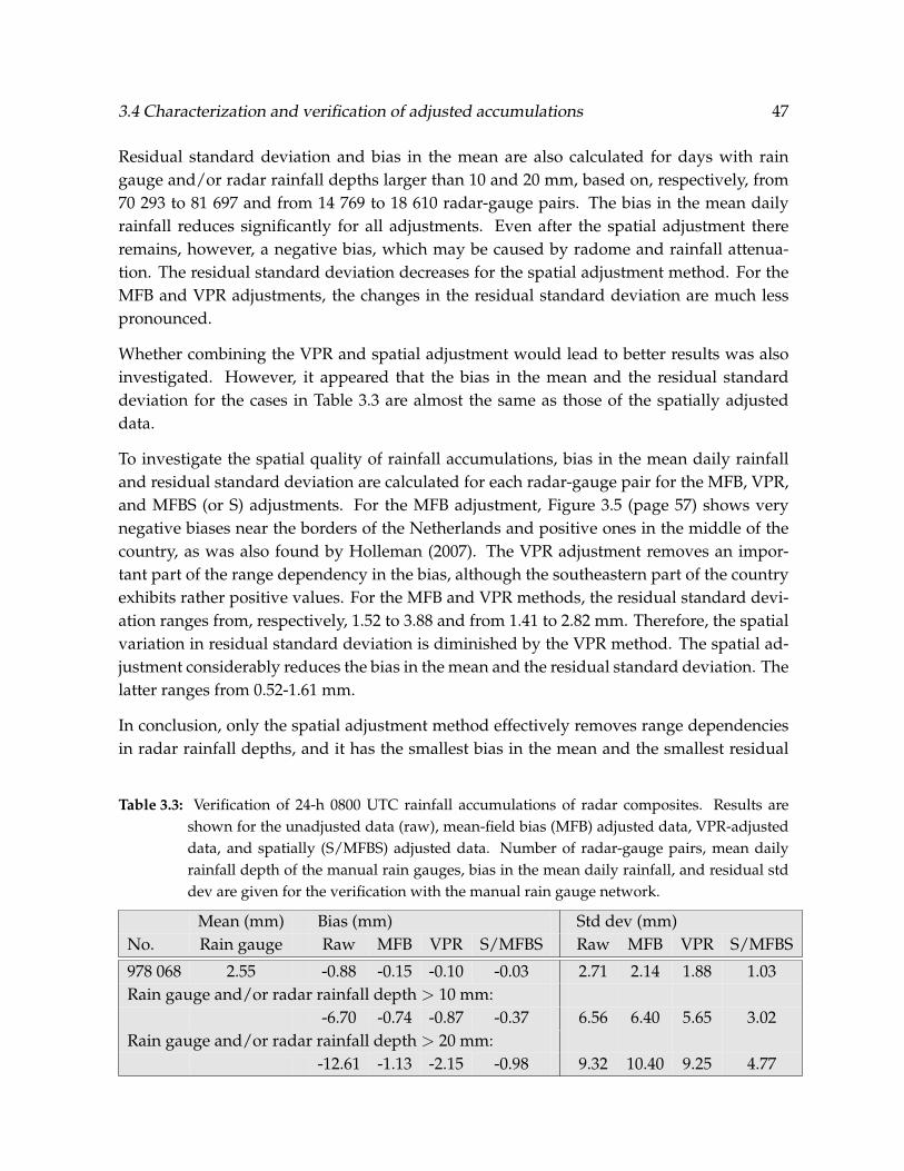
3.4 Characterization and verification of adjusted accumulations 47
Residual standard deviation and bias in the mean are also calculated for days with rain
gauge and/or radar rainfall depths larger than 10 and 20 mm, based on, respectively, from
70 293 to 81 697 and from 14 769 to 18 610 radar-gauge pairs. The bias in the mean daily
rainfall reduces significantly for all adjustments. Even after the spatial adjustment there
remains, however, a negative bias, which may be caused by radome and rainfall attenua-
tion. The residual standard deviation decreases for the spatial adjustment method. For the
MFB and VPR adjustments, the changes in the residual standard deviation are much less
pronounced.
Whether combining the VPR and spatial adjustment would lead to better results was also
investigated. However, it appeared that the bias in the mean and the residual standard
deviation for the cases in Table 3.3 are almost the same as those of the spatially adjusted
data.
To investigate the spatial quality of rainfall accumulations, bias in the mean daily rainfall
and residual standard deviation are calculated for each radar-gauge pair for the MFB, VPR,
and MFBS (or S) adjustments. For the MFB adjustment, Figure 3.5 (page 57) shows very
negative biases near the borders of the Netherlands and positive ones in the middle of the
country, as was also found by Holleman (2007). The VPR adjustment removes an impor-
tant part of the range dependency in the bias, although the southeastern part of the country
exhibits rather positive values. For the MFB and VPR methods, the residual standard devi-
ation ranges from, respectively, 1.52 to 3.88 and from 1.41 to 2.82 mm. Therefore, the spatial
variation in residual standard deviation is diminished by the VPR method. The spatial ad-
justment considerably reduces the bias in the mean and the residual standard deviation. The
latter ranges from 0.52-1.61 mm.
In conclusion, only the spatial adjustment method effectively removes range dependencies
in radar rainfall depths, and it has the smallest bias in the mean and the smallest residual
Table 3.3: Verification of 24-h 0800 UTC rainfall accumulations of radar composites. Results are
shown for the unadjusted data (raw), mean-field bias (MFB) adjusted data, VPR-adjusted
data, and spatially (S/MFBS) adjusted data. Number of radar-gauge pairs, mean daily
rainfall depth of the manual rain gauges, bias in the mean daily rainfall, and residual std
dev are given for the verification with the manual rain gauge network.
Mean (mm) Bias (mm) Std dev (mm)
No. Rain gauge Raw MFB VPR S/MFBS Raw MFB VPR S/MFBS
978 068 2.55 -0.88 -0.15 -0.10 -0.03 2.71 2.14 1.88 1.03
Rain gauge and/or radar rainfall depth > 10 mm:
-6.70 -0.74 -0.87 -0.37 6.56 6.40 5.65 3.02
Rain gauge and/or radar rainfall depth > 20 mm:
-12.61 -1.13 -2.15 -0.98 9.32 10.40 9.25 4.77

48 Chapter 3 — Derivation of a 10-year radar-based climatology of rainfall
standard deviation. The VPR adjustment is not employed in the remainder of this chapter,
given that it performs worse than the spatial adjustment method. The hourly MFB adjust-
ment is considered further because this method is expected to show good results in the
verification of short-duration rainfall.
3.4.3 Verification with automatic rain gauges
The 10-yr data set of radar-derived composited rainfall accumulations is verified with the
automatic rain gauge network for durations D of 1, 2, 4, 8, 12, and 24 h, where the accu-
mulations are obtained for every clock-hour. Again, the residuals are calculated for each
radar-gauge pair. Raw, MFB-adjusted, S-adjusted, and MFBS-adjusted radar rainfall accu-
mulations are verified.
As seen in Table 3.4, the bias in the mean 1-h rainfall depth is reduced from -0.03 mm for the
raw data to 0.00 and 0.01 mm for, respectively, the MFB and both spatial adjustment meth-
ods, the mean 1-h gauge rainfall depth being 0.10 mm. The adjustments reduce the residual
standard deviation. Residual standard deviation and bias in the mean are also calculated
for hours with rain gauge and/or radar rainfall depths larger than 5 and 10 mm, based on,
respectively, 4414 to 5454 and 749 to 909 radar-gauge pairs. The adjustments clearly dimin-
ish the bias in the mean; however, the reduction in the residual standard deviation is less
pronounced. The daily adjustment method S results in less-negative biases than the hourly
adjustment method MFB, which is, however, more successful in reducing the residual stan-
dard deviations. Because of the variable temporal distribution of rainfall amounts over a
day and the possible alternation of convective and stratiform rainfall, a daily adjustment
factor field will not always result in properly adjusted 1-h rainfall depths. The combined
hourly and daily adjustment (MFBS) method gives the smallest bias in the mean and the
smallest residual standard deviation. This implies that a daily adjustment using a dense
gauge network, which improves the spatial quality of the rainfall depths, has added value
if applied to 1-h rainfall depths that are already MFB adjusted.
The negative bias in the mean daily rainfall for the verification with manual gauges (Table
3.3) changes into 0.12 mm for both spatial adjustment methods (Table 3.4). This is probably
due to the bias in the automatic rain gauge measurements with respect to those from the
manual rain gauges. To investigate the validity of this, the differences between the 24-h ac-
cumulations from manual and automatic rain gauges within a 2.4-km radius are calculated
for the entire period 1998-2007 using, on average, 21 pairs per day. These differences are, on
average, 0.14 mm, which implies that manual rain gauge depths are systematically higher
relative to the automatic rain gauge depths. According to Chapter 2, where 12 stations from
the two rain gauge networks were utilized, annual rainfall sums from manual rain gauges
are, on average, 5% larger than those from collocated automatic rain gauges. This corre-
sponds to the change in bias between the verification with manual and automatic gauges
of 6% of the mean daily gauge rainfall depth, and this change can therefore be attributed
to the automatic rain gauges having a different measurement technique than the manual

3.4 Characterization and verification of adjusted accumulations 49
ones. The standard deviation of the differences between manual and automatic gauges is
1.06 mm. This indicates that an important part of the standard deviation of the differences
between the 24-h MFBS radar and automatic rain gauge accumulations (1.32 mm) is caused
by subpixel rainfall variations.
Next, for each duration the residuals are ranked in increasing order and the values belonging
to the 2.5th, 50th (median), and 97.5th percentiles are determined and plotted in Figure 3.6.
For the raw radar data, the interval between the 2.5th and 97.5th percentiles of the residuals
is wide, 9.4 mm for D = 24 h, and the distribution is negatively skewed, implying that with
respect to rain gauges the underestimates are more severe than the overestimates. Note that
also values of (near) zero rainfall, which occur so frequently that the median is close to zero,
are used to construct Figure 3.6.
For D = 24 h, the percentile interval decreases to 4.9 mm for the MFBS adjustment method
and the asymmetry of the distribution of the residuals has disappeared. Similar results are
obtained for durations that are less than 24 h, although the percentile interval is reduced
only slightly for D = 1-4 h. Germann et al. (2006) also find an underestimation for raw daily
radar precipitation depths that is considerably reduced if, among other things, a real-time
VPR adjustment and a global bias correction are applied.
For D = 24 h, the residual standard deviation decreases from 2.58 (raw) to 1.81 (MFB),
1.38 (S), and 1.32 (MFBS) mm; see Table 3.4. If the residuals were normally distributed, the
interval between the 2.5th and 97.5th percentiles would be equal to 4 times the standard
deviation. This would result in a percentile interval of 10.3 (raw) or 5.3 (MFBS) mm. These
Table 3.4: Verification of 1-h and 24-h composited rainfall accumulations for every clock-hour. Re-
sults are shown for the unadjusted data (raw), MFB-adjusted data, S-adjusted data, and
MFBS-adjusted data. Number of radar-gauge pairs, mean rainfall depth of the automatic
rain gauges, bias in the mean rainfall, and residual std dev are given for the verification
with the automatic rain gauge network.
Mean (mm) Bias (mm) Std dev (mm)
No. Rain gauge Raw MFB S MFBS Raw MFB S MFBS
1-h rainfall depths
2 336 315 0.10 -0.03 0.00 0.01 0.01 0.35 0.29 0.30 0.27
Rain gauge and/or radar rainfall depth > 5 mm:
-3.81 -0.82 -0.80 -0.51 4.60 3.96 4.32 3.80
Rain gauge and/or radar rainfall depth > 10 mm:
-8.59 -3.16 -2.69 -2.06 6.98 6.63 7.58 6.55
24-h rainfall depths
2 250 878 2.41 -0.75 -0.04 0.12 0.12 2.58 1.81 1.38 1.32

50 Chapter 3 — Derivation of a 10-year radar-based climatology of rainfall
−8
−6
−4
−2
02
Duration (h)
Rra
wc
− G
(m
m)
−8
−6
−4
−2
02
Duration (h)
Rra
wc
− G
(m
m)
−8
−6
−4
−2
02
Duration (h)
Rra
wc
− G
(m
m)
12 4 8 12 242.
5%50
%97
.5%
−8
−6
−4
−2
02
Duration (h)
RM
FB
Sc
− G
(m
m)
−8
−6
−4
−2
02
Duration (h)
RM
FB
Sc
− G
(m
m)
−8
−6
−4
−2
02
Duration (h)
RM
FB
Sc
− G
(m
m)
12 4 8 12 24
2.5%
50%
97.5
%
Figure 3.6: The 2.5th, 50th (median), and 97.5th percentiles of the residuals (mm) in the verification
with automatic rain gauges plotted against duration for the composited (left) raw and
(right) MFBS-adjusted radar data.
values are higher than those given above, implying that the residuals are not well approx-
imated by the normal distribution, which situation is caused by the frequent occurrence of
(near) zero rainfall and, for the raw radar data, also by the asymmetry.
From the verification with automatic gauges, it appears that the MFBS adjustment performs
well on both daily and subdaily accumulations and generally removes the systematic un-
derestimation of precipitation by radar more effectively than do the other adjustments.
3.5 Long-term radar rainfall statistics
The Netherlands, which is located in the midlatitudes, has a temperate climate with pre-
vailing westerly winds. The mean annual rainfall varies spatially from 675 to 925 mm. In
this section, the MFBS-adjusted radar rainfall climatology is analyzed to derive exceedance
probabilities, mean annual rainfall frequencies, maximum rainfall depths, and spatial cor-
relations. In comparisons with climatologies from gauge data, these data were only used if
the corresponding radar data were available, except for exceedance probabilities.
3.5.1 Empirical exceedance probabilities
Based on the radar data set, empirical exceedance probabilities of rainfall are calculated.
Only the radar data above the land surface of the Netherlands are selected. Using the rainfall
depths from all radar pixels (6190), rainfall frequencies are computed for classes of 1 mm.
Exceedance frequencies are subsequently calculated and are scaled with the sum of all fre-
quencies, so that empirical exceedance probabilities of rainfall depths are obtained, which
are shown in Figure 3.7 for different durations. For example, the left panel demonstrates
for the spatially adjusted radar data that a 24-h 0800-0800 UTC rainfall depth of 100 mm has

3.5 Long-term radar rainfall statistics 51
an exceedance probability of approximately 1.2×10⁻⁵, implying that on average this rainfall
depth is exceeded approximately once in 8.1×10⁴ days (≈ 223 yr) in an arbitrary radar pixel.
These exceedance probabilities are spatial averages over the Netherlands and are assumed
to be independent of season. Deviations from these averages are probably limited, because
the Netherlands is a relatively small and flat country.
Figure 3.7 shows that the exceedance probabilities of 24-h 0800-0800 UTC rainfall from the
adjusted radar data (MFB and MFBS) are, in general, in good correspondence with those
based on the manual rain gauges, whereas the use of raw radar data results in much lower
exceedance probabilities. Therefore, adjustment of radar data with rain gauges is a pre-
requisite to obtain reliable exceedance probabilities of rainfall. Even the MFB adjustment
method removes the systematic underestimation of exceedance probabilities; however, large
exceedance probabilities are found at high rainfall depths.
To explain the good correspondence between the exceedance probabilities from the adjusted
radar data and the manual rain gauge data, the standard deviations of the 24-h 0800-0800
UTC rainfall depths are calculated. These are 4.81, 4.71, and 4.77 mm for, respectively, the
rain gauge data, the MFB-adjusted, and the MFBS-adjusted radar data. The differences
among these standard deviations are small, even though the standard deviations of the
residuals in Tables 3.3 and 3.4 are still substantial in the case of MFB and MFBS adjustments
(about 38%-44% and 21%-27% of the standard deviation of the daily manual rain gauge
depths). These residuals contain a component representing the subpixel rainfall variation
and a remaining bias of radar rainfall (Ciach and Krajewski, 1999). Because of the first com-
ponent the variance of the rain gauge rainfall is larger than that of the true area-averaged
rainfall, whereas because of the second component the variance of the radar rainfall is larger
than that of the true area-averaged rainfall. However, the increase in standard deviation due
to adding a random component to the true area-averaged rainfall is usually limited. For in-
stance, if the standard deviation of the random component is 20% of the standard deviation
of the true area-averaged rainfall, the increase is only 2%. This explains the small differences
between the radar and gauge standard deviations.
Figure 3.7 also gives the exceedance probabilities for the 1-h rainfall depths. Again the MFB
adjustment is successful in removing the systematic underestimation of exceedance proba-
bilities in the raw radar data. However, an important shortcoming of the MFB method is the
large exceedance probabilities at high rainfall depths. It appears that the MFB adjustment
creates a number of outliers. Therefore, it is important to apply a daily spatial adjustment af-
ter the mean-field bias adjustment. Then, the number of outliers is limited. The exceedance
probabilities after the spatial adjustments are in good correspondence with those from the
automatic rain gauge data up to a rainfall amount of 20 mm.
Figure 3.8 gives the exceedance probabilities for 1-, 2-, 4-, 8-, 12-, and 24-h accumulated rain-
fall for the MFBS-adjusted radar data. For instance, a 1-h rainfall depth of 5 mm is exceeded

52 Chapter 3 — Derivation of a 10-year radar-based climatology of rainfall
1 2 5 10 20 50
24−h rainfall depth (mm)
Em
piric
al e
xcee
danc
e pr
obab
ility Gauge, manual
1 2 5 10 20 50
24−h rainfall depth (mm)
Em
piric
al e
xcee
danc
e pr
obab
ility
Radar, raw
1 2 5 10 20 50
24−h rainfall depth (mm)
Em
piric
al e
xcee
danc
e pr
obab
ility
Radar, MFB
1 2 5 10 20 50
24−h rainfall depth (mm)
Em
piric
al e
xcee
danc
e pr
obab
ility
Radar, MFBS
100
10−−2
10−−4
10−−6
1 2 5 10 20 50
1−hour rainfall depth (mm)E
mpi
rical
exc
eeda
nce
prob
abili
ty
1 2 5 10 20 50
1−hour rainfall depth (mm)E
mpi
rical
exc
eeda
nce
prob
abili
ty
1 2 5 10 20 50
1−hour rainfall depth (mm)E
mpi
rical
exc
eeda
nce
prob
abili
ty
1 2 5 10 20 50
1−hour rainfall depth (mm)E
mpi
rical
exc
eeda
nce
prob
abili
ty
1 2 5 10 20 50
1−hour rainfall depth (mm)E
mpi
rical
exc
eeda
nce
prob
abili
ty Gauge, automaticRadar, rawRadar, MFBRadar, SRadar, MFBS
100
10−−2
10−−4
10−−6
Figure 3.7: Exceedance probabilities of (left) 24-h 0800-0800 UTC and (right) 1-h rainfall sums over
the period 1998-2007.
on average approximately once in 610 clock-hours (≈ 25 days). These exceedance proba-
bilities are based on the D-hour accumulations for every clock-hour. This provides more
accurate estimates than the use of nonoverlapping D-hour accumulations. In the latter case,
there is even a risk that the line of, for instance, the 8-h exceedance probabilities crosses that
of the 12-h exceedance probabilities because the amount in the 1600-0000 UTC interval can
exceed the amounts in the 0800-2000 and 2000-0800 UTC intervals. Therefore, exceedance
probabilities are calculated using accumulations for every clock-hour.
3.5.2 Rainfall frequency and maximum rainfall depths
Now that the exceedance probabilities have shown a reasonable correspondence with those
from rain gauges, the spatial distribution of extreme rainfall is investigated in this section.
Figure 3.9 displays the maximum daily (0800-0800 UTC) rainfall sums from manual rain
gauge data (a) and MFBS-adjusted radar data from the corresponding pixel (b) for the period
1998-2007 and demonstrates a good resemblance between both. Differences can partly be
attributed to spatial representativeness errors, since the radar image has a 2.4-km spatial
resolution and the rain gauge is a point measurement (Kitchen and Blackall, 1992).
For the radar data also the maximum 1-h rainfall sums are plotted (c), which is, at an ac-
ceptable spatial resolution, not possible for the rain gauge data. The maximum 1-h rainfall
sum shows a strong spatial variation, with values ranging from 12 to 127 mm (only five
values exceed 100 mm). This is mainly due to the long upper tail of the distribution of the
hourly precipitation amounts and some artificially large values. Figure 3.9 also gives the
mean annual number of days with more than 10 mm and hours with more than 5 mm of
rain. The radar-based mean annual number of days (e) corresponds well to that from the

3.5 Long-term radar rainfall statistics 53
1 2 5 10 20 50
Rainfall depth (mm)
Em
piric
al e
xcee
danc
e pr
obab
ility
1 2 5 10 20 50
Rainfall depth (mm)
Em
piric
al e
xcee
danc
e pr
obab
ility
1 2 5 10 20 50
Rainfall depth (mm)
Em
piric
al e
xcee
danc
e pr
obab
ility
1 2 5 10 20 50
Rainfall depth (mm)
Em
piric
al e
xcee
danc
e pr
obab
ility
1 2 5 10 20 50
Rainfall depth (mm)
Em
piric
al e
xcee
danc
e pr
obab
ility
1 2 5 10 20 50
Rainfall depth (mm)
Em
piric
al e
xcee
danc
e pr
obab
ility
24 h
12 h8 h
4 h
2 h
1 h
Radar, MFBS100
10−−2
10−−4
10−−6
Figure 3.8: Exceedance probabilities of 1-, 2-, 4-, 8-, 12-, and 24-h rainfall sums over the period 1998-
2007 for the MFBS adjustment method.
rain gauges (d). The mean annual number of clock-hours with more than 5 mm (f) displays
a large spatial variability and ranges from 8 to a value as high as 22 (not shown: one outlier
of 28). This is mainly a consequence of the large year-to-year variation and weak spatial
correlation of such events. For only 5.4% of the pixels, the mean annual number of hours
with more than 5 mm of rain differs by more than 2 times its standard deviation from the
countrywide mean annual number of exceedances, implying that the spatial variability can
be attributed to randomness. This percentage is larger for, respectively, the 24-h radar (17%)
and rain gauge (22%) depths. Earlier studies that show the spatial distribution of rainfall
frequencies are Croft and Shulman (1989) and Baeck and Smith (1995).
3.5.3 Spatial correlation
The spatial correlation of precipitation is investigated for different timescales. In Figure 3.10
cross correlations between precipitation depths are plotted against distance for MFBS-adjusted
radar data (D = 1 and 24 h) and automatic rain gauges (D = 24 h). Only radar data at the
location of the automatic rain gauges are selected. The exponential decay of precipitation
depths with interpixel or intergauge distance can be described reasonably with
ρ(x) = exp
[−
(x
x0
)s0]
, (3.16)
where ρ(x) is the correlation at distance x (km), x0 a scale parameter (km) and s0 is a shape
parameter. The influence of anisotropy is not considered. The correlation coefficients were
estimated with the method of nonlinear least squares. Ciach and Krajewski (2006) employed
a similar model for spatial correlations in small-scale rainfall. A rain gauge depth is only

54 Chapter 3 — Derivation of a 10-year radar-based climatology of rainfall
1998−2007
Max
imum
24−
hour
rai
nfal
l dep
th (
mm
)a)
Gauge
b)
Radar20
40
60
80
100
120
140
1998−2007
Max
imum
1−
hour
rai
nfal
l dep
th (
mm
)
c)
Radar20
40
60
80
100
120
140M
ean
annu
al fr
eque
ncy
of 2
4−ho
ur d
epth
s >
10
mm d)
Gauge
e)
Radar18
20
22
24
26
28
30
32
34
Mea
n an
nual
freq
uenc
y of
1−
hour
dep
ths
> 5
mm f)
Radar8
10
12
14
16
18
20
22
Figure 3.9: (top) Maximum rainfall depths over the period 1998-2007 and (bottom) mean annual
number of days with more than 10 mm and hours with more than 5 mm, based on the
24-h accumulations (0800-0800 UTC) from (a),(d) manual rain gauges and (b),(e) radar
(MFBS adjusted) and on (c),(f) the 1-h MFBS-adjusted radar accumulations.
taken into account if the radar depth is available and vice versa. Further, only precipitation
depths of at least 0.5 mm in 1 or 24 h are used in the estimation of the correlation. The radar
measures over 5.7-km2 areas, and the rain gauge produces point measurements in space.
Because of this, rain gauge measurements are more influenced by small-scale events and
have therefore a slightly lower spatial correlation than the radar-based accumulations. Fur-
ther, the correlations for D = 24 h are much higher than those for D = 1 h. This is related
to the spatial-temporal correlation structure of rainfall fields. For instance, the spatial corre-
lation between the 1- and 24-h accumulations would be the same if there were no temporal
correlation, which is obviously not the case.

3.6 Conclusions and recommendations 55
0.0
0.2
0.4
0.6
0.8
1.0
Distance (km)
Cor
rela
tion
0 50 100 150 200 250 300
s0 =
x0 =
0.43
28km
Gauge, 1 h 0.0
0.2
0.4
0.6
0.8
1.0
Distance (km)C
orre
latio
n
0 50 100 150 200 250 300
s0 =
x0 =
0.5
36km
Radar, MFBS, 1 h
0.0
0.2
0.4
0.6
0.8
1.0
Distance (km)
Cor
rela
tion
0 50 100 150 200 250 300
s0 =
x0 =
0.7
170 km
Radar, MFBS, 24 h
Figure 3.10: Correlation between (left) 1-h rain gauge, (right) 1-h radar, and (bottom) 24-h radar pre-
cipitation depths as a function of distance.
3.6 Conclusions and recommendations
Based on data from two weather radars, a 10-yr rainfall climatology was constructed for
the Netherlands. The radar data were corrected for occultation and anomalous-propagation
ground clutter. Using manual rain gauges, two daily adjustment methods were applied
separately and verified: 1) a VPR and bias adjustment and 2) a spatial adjustment. The 24-h
(0800-0800 UTC) spatial adjustment field was also applied to the 1-h unadjusted radar data.
Automatic rain gauges were employed to derive MFB-adjusted 1-h precipitation depths.
The spatial and MFB adjustment methods were combined to derive 1-h rainfall depths. For

56 Chapter 3 — Derivation of a 10-year radar-based climatology of rainfall
0800 UTC 20031231 − 0800 UTC 20040131
Pre
cipi
tatio
n de
pth
(mm
)
a) b) c)
d) e) f)
20
40
60
80
100
120
140
160
Figure 3.3: Monthly rainfall depths for January 2004 for a) the raw De Bilt radar data, b) the raw De
Bilt radar data corrected for occultation, c) the manual rain gauges (interpolated), d) the
raw radar composite corrected for occultation, e) the VPR-adjusted radar composite, and
f) the spatially (S/MFBS) adjusted composite. For this month both radars have a data
availability of 100%.
each clock-hour, 2-, 4-, 8-, 12-, and 24-h accumulations were derived from the 1-h rainfall
composites. The accumulations were verified with rainfall depths from automatic (D ≤ 24 h)
and manual (D = 24 h) rain gauge networks. The newly developed combination of an
hourly mean-field bias and a daily spatial adjustment method gave the best verification re-
sults. Therefore, this data set was used to derive exceedance probabilities, mean annual
frequencies, maximum rainfall depths, and spatial correlations.
This chapter contains a description and an analysis of one of the longest radar data sets de-
scribed in the literature. The data set has a high resolution, which is a prerequisite to derive
accurate rainfall climatologies. Also, subdaily rainfall depths are obtained. The combination
of an hourly mean-field bias adjustment and a daily spatial adjustment is a novel approach
that improves the quality of subdaily radar rainfall depths considerably. An improved spa-
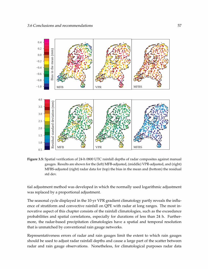
3.6 Conclusions and recommendations 57
Bia
s in
the
mea
n (m
m)
MFB VPR−1.0
−0.8
−0.6
−0.4
−0.2
0.0
0.2
0.4
MFBS
Res
idua
l sta
ndar
d de
viat
ion
(mm
)
MFB VPR0.5
1.0
1.5
2.0
2.5
3.0
3.5
4.0
MFBS
Figure 3.5: Spatial verification of 24-h 0800 UTC rainfall depths of radar composites against manual
gauges. Results are shown for the (left) MFB-adjusted, (middle) VPR-adjusted, and (right)
MFBS-adjusted (right) radar data for (top) the bias in the mean and (bottom) the residual
std dev.
tial adjustment method was developed in which the normally used logarithmic adjustment
was replaced by a proportional adjustment.
The seasonal cycle displayed in the 10-yr VPR gradient climatology partly reveals the influ-
ence of stratiform and convective rainfall on QPE with radar at long ranges. The most in-
novative aspect of this chapter consists of the rainfall climatologies, such as the exceedance
probabilities and spatial correlations, especially for durations of less than 24 h. Further-
more, the radar-based precipitation climatologies have a spatial and temporal resolution
that is unmatched by conventional rain gauge networks.
Representativeness errors of radar and rain gauges limit the extent to which rain gauges
should be used to adjust radar rainfall depths and cause a large part of the scatter between
radar and rain gauge observations. Nonetheless, for climatological purposes radar data

58 Chapter 3 — Derivation of a 10-year radar-based climatology of rainfall
should be adjusted with rain gauges or disdrometers in a sensible manner, because of the
possible errors in QPE with radar.
Errors in QPE not specifically accounted for in this chapter are attenuation, bright band ef-
fects, and advection of precipitation. However, the spatial adjustment will probably correct
an important part of these errors. The VPR adjustment method is partially successful in cor-
recting for spatial differences in the quality of radar rainfall depths. The VPR adjustment is
a mean-range correction, whereas in reality large spatial variations in VPR gradients can oc-
cur. The spatial adjustment is clearly more successful in adjusting the radar rainfall depths
and results in a data set with a spatially homogeneous quality.
Until February of 2001 the results were based on the De Bilt radar only. Some hardware
calibration issues were addressed, such as the exclusion of radar data because of an elevation
bias and the identification of systematically lower radar rainfall depths from the middle of
2004 caused by a sudden change in the calibration of the radar receiver. The radars were
not replaced or moved during the 10-yr period, nor was the scanning strategy changed.
The effective length of the time series is approximately 8 yr. Verification with rain gauges
confirms the quality of the radar precipitation climatology.
If it were available, using a volumetric data set of radar reflectivities would increase the
possibilities to improve the quality of QPE. For instance, a VPR correction could be applied
using radar reflectivities instead of rain gauges (Vignal et al., 2000; Vignal and Krajewski,
2001). Further, an attenuation correction could be developed using polar data from one
elevation. An advantage is that these corrections can be employed in real-time.
This data set is also potentially useful for the investigation of rainfall parameterization in
mesoscale weather and climate models and as a test bed for the development of rainfall
retrieval algorithms for satellite-based rainfall estimates, such as the Global Precipitation
Measurement Mission.
The next step in the use of the radar rainfall climatology is to calculate probabilities of ex-
treme rainfall (e.g., for use in the design of hydraulic structures). This would enable us to
study the statistics of extreme areal rainfall for durations of less than 24 h, which is difficult
to achieve with rain gauges. Attention will also be given to subhourly rainfall accumula-
tions. Furthermore, statistics of extreme rainfall will be modeled as a function of area size,
and regional variability in extreme rainfall will be studied.
Acknowledgements
The authors gratefully acknowledge the comments given by Remko Uijlenhoet (Hydrology
and Quantitative Water Management Group, Wageningen University). We also thank the
two anonymous reviewers for their critical comments. Last, we thank Rudolf van Westrhenen
(KNMI) for archiving more than 5 yr of radar data.

Chapter 4
Extreme rainfall analysis and estimation
of depth-duration-frequency curves using
weather radar1
Abstract
Rain gauge data are often employed to estimate the rainfall depth for a given return period. How-
ever, the number of rain gauge records of short-duration rainfall, such as 15 min, is sparse. The
obvious advantage of radar data over most rain gauge networks is their higher temporal and spatial
resolution. Furthermore, the current quality of quantitative precipitation estimation with radar and
the length of the available time series make it feasible to calculate radar-based extreme rainfall statis-
tics. In this chapter an 11-year radar data set of precipitation depths for durations of 15 min to 24 h
is derived for the Netherlands (3.55 × 10⁴ km2). The radar data are adjusted using rain gauges by
combining an hourly mean-field bias adjustment with a daily spatial adjustment. Assuming a Gener-
alized Extreme Value (GEV) distribution, the index flood method is used to describe the distribution
of the annual radar rainfall maxima. Regional variability in the GEV location parameter is studied.
GEV parameters based on radar and rain gauge data are compared and turn out to be in reasonable
agreement. Furthermore, radar rainfall depth-duration-frequency (DDF) curves and their uncertain-
ties are derived and compared with those based on rain gauge data. Although uncertainties become
large for long durations, it is shown that radar data are suitable to construct DDF curves.
1Water Resources Research, 2009, doi:10.1029/2009WR007869, 45, W10424, by Aart Overeem, Adri Buishand
and Iwan Holleman.
59

60 Chapter 4 — Extreme rainfall analysis and estimation of DDF curves using radar
4.1 Introduction
Rain gauge data are often utilized to estimate rainfall depths for given probabilities of ex-
ceedance. For example, annual daily rainfall maxima are extracted from a 50-year record
and subsequently an extreme value distribution, such as the Generalized Extreme Value
(GEV) distribution, is fitted to these annual maxima. Next, the fitted distribution is used to
calculate the rainfall depth for a given return period, which is, for instance, of importance
for design purposes in water management.
Generally, only rain gauge data are used to obtain statistics of extreme rainfall, often for
durations of 24 h or longer. However, the number of rain gauge records of short-duration
rainfall, such as 15 min, is sparse. Further, the spatial density of rain gauge networks is often
too low to obtain reliable statistics of extreme areal rainfall for subhourly durations.
Although Collier (1989) already mentioned the potential of weather radar data for extreme
value analyses and weather radars are nowadays widely used in real-time quantitative pre-
cipitation estimation (QPE), radar data have only been used in some studies to derive statis-
tics of extreme rainfall. Durrans et al. (2002) estimated rainfall depth-area relationships for
different exceedance frequencies by fitting a Gumbel distribution to annual radar rainfall
maxima for durations of 1, 2 and 4 h using an 8-year data set, the largest area size being ap-
proximately 1300 km2. Allen and DeGaetano (2005b) estimated extreme areal precipitation
depths for return periods of 2, 5 and 10 years using a 5-year data set of 24-h accumulated
rainfall for New Jersey and North Carolina (United States) for area sizes up to 20 000 km2.
Lombardo et al. (2006) used radar data to estimate areal reduction factors for durations of 1
to 120 min and return periods of 2 to 50 years for area sizes ranging from 1 to 900 km2.
The obvious advantage of radar data with respect to most rain gauge networks is their
higher temporal and spatial resolution. Further, the current quality of QPE with radar and
the length of available time series make it feasible to calculate radar-based extreme rainfall
statistics. Possible limitations of the aforementioned studies are heterogeneities caused by
continual improvements to the data processing algorithms (Durrans et al., 2002), the small
number of levels (13) of daily rainfall accumulations (Allen and DeGaetano, 2005b), and the
lack of an adjustment of radar rainfall depths using rain gauges (Lombardo et al., 2006).
In this chapter an 11-year radar data set of precipitation depths for durations of 15 min to
24 h is derived for the Netherlands (3.55 × 10⁴ km2), a densely populated country with over
16 million inhabitants. The radar data are adjusted by combining an hourly mean-field bias
adjustment using an automatic rain gauge network and a daily spatial adjustment employ-
ing a dense manual gauge network. The adjustment procedures and the verification of this
data set are described in Chapter 3. The characteristics of annual maximum precipitation
depths are investigated for each radar pixel (approximately 6 km2). Subsequently, GEV dis-
tributions are fitted to these annual maxima to derive the rainfall depths for various return
periods. To obtain accurate estimates of the parameters of this distribution from an 11-year

4.2 Radar and rain gauge data 61
0 50
N
km
De Bilt
Den Helder
North Sea
0 50
N
km
North Sea
Figure 4.1: Maps of the Netherlands with left the locations of the weather radars in De Bilt and Den
Helder, their 200-km range (circles), and the 33 automatic rain gauges (squares) and right
the locations of the 326 manual rain gauges.
data set, the index flood method is applied. This method assumes that only the GEV loca-
tion parameter varies spatially. A comparison is made between the parameters of the GEV
distribution based on radar and on gauge data. Further, rainfall depth-duration-frequency
(DDF) curves are derived. DDF curves describe rainfall depth as a function of duration for
given return periods or probabilities of exceedance. To the authors’ knowledge, this study
is the first in which DDF curves are derived from radar data. The DDF curves and their
uncertainties are calculated following a similar approach as developed in Chapter 2.
This chapter is organized as follows. Section 4.2 gives a description of the radar and rain
gauge data. In Section 4.3 a data set of adjusted radar-derived rainfall accumulations is con-
structed. Some characteristics of annual maxima are discussed in Section 4.4. In Section 4.5
regional variability in extreme rainfall statistics is studied. In Section 4.6 extreme rainfall
statistics based on radar and on gauge data are compared. GEV parameters are modeled as
a function of duration in Section 4.7 to derive radar-based DDF curves and their uncertain-
ties in Section 4.8. The chapter ends with a discussion and conclusions.
4.2 Radar and rain gauge data
A weather radar transmits radio-frequency waves into the atmosphere and receives the re-
flected signals from hydrometeors as echo powers, from which reflectivity factors are cal-
culated. From 1998 to 2008, horizontal cross sections of radar reflectivity factor at constant
altitude, called pseudo constant altitude plan position indicators (pseudo CAPPI), were ob-
tained from the two C-band Doppler weather radars in the Netherlands. The radars, which
are operated by the Royal Netherlands Meteorological Institute (KNMI), are located in De
62 Chapter 4 — Extreme rainfall analysis and estimation of DDF curves using radar
Bilt (52.10◦ N, 5.18◦ E, 44 m above mean sea level) and Den Helder (52.96◦ N, 4.79◦ E, 51 m
above mean sea level; see Figure 4.1). Ground clutter was removed from the pseudo CAPPI
images, which have a 2.4-km horizontal resolution and a 5-min temporal resolution, using
the procedure described in Holleman and Beekhuis (2005). To suppress echoes caused by
hail or strong residual ground clutter, reflectivities above 55 dBZ (≈ 100 mm h−1) were set
to 55 dBZ. A rainfall intensity of 96 mm h−1 is exceeded approximately once in 6.6 years at
an arbitrary pixel. Next, rainfall intensities R (mm h−1) were calculated from the reflectivity
factors Z (mm6 m−3) with a fixed Z-R relationship (Marshall et al., 1955),
Z = 200R1.6. (4.1)
The obtained rainfall intensities range from 0.1 to 100 mm h−1 and have a resolution of
97 levels. Subsequently, 1-h rainfall depths were derived from rainfall intensities for each
clock-hour if at least 10 images (minimum availability of 83.3%) were available. A five-pixel
median filter on nearest-neighbor pixels was applied to the depths to remove local outliers
caused by accumulated residual ground clutter. The range of the radar accumulation images
was limited to 200 km and the data were corrected for occultation due to tall buildings in the
vicinity of the radar. Accumulation images from the individual radars were combined into
one composite using a weighting factor depending on the range from the radar. Chapter 3
gives a more elaborate description of the radar data set based on 1998-2007, but do not
derive subhourly rainfall accumulations. The present chapter uses the same methodology
to also obtain adjusted 5-min rainfall data. Only those 5-min data were selected for which
the corresponding 1-h depth (for a clock-hour) was available. The data set of composites
covers the entire land surface of the Netherlands (≈ 3.55 × 10⁴ km2) and has an effective
length of approximately 9 years, of which 3 years are based on the De Bilt radar only.
In this chapter, rain gauges, which are considered to produce accurate point measurements,
are used to improve the quality of QPE with radar. Data from an automatic network of 33
rain gauges (≈ 1 station per 1000 km2) and a manual network of 326 rain gauges (≈ 1 station
per 100 km2) were employed. Figure 4.1 displays the locations of the rain gauges. The
automatic rain gauges measured 1-h rainfall depths for each clock-hour, while from the
manual rain gauges 24-h 08-08 UTC rainfall depths were obtained. For more details on the
rain gauge networks, see Chapter 3.
4.3 Adjustment of radar-based rainfall depths
4.3.1 Adjustment method
A radar indirectly measures rainfall intensities at heights of a few hundred meters to several
kilometers above ground level. This may give rise to errors in QPE with radar, such as
those caused by a nonuniform vertical profile of reflectivity or variability of the drop-size
distribution. Besides, the radar signal is attenuated in the case of strong precipitation or a
wet radome. Therefore, it is necessary to adjust the radar data to derive a high-quality radar-
based rainfall climatology. A detailed discussion of QPE with radar and their associated

4.3 Adjustment of radar-based rainfall depths 63
errors can be found in Joss and Waldvogel (1990) and Doviak and Zrnic (1993).
The methods used to adjust the radar rainfall depths are described in detail in Chapter 3.
They show that combining an hourly mean-field bias adjustment with a daily spatial ad-
justment results in high-quality 1- to 24-h radar rainfall depths (for each clock-hour). The
manual gauge network is used to apply a spatial adjustment to the unadjusted 24-h 08 UTC
rainfall depths. A spatial adjustment factor field is calculated by dividing the interpolated
manual gauge precipitation depths G by the corresponding interpolated raw radar precipi-
tation depths Rcraw:
FcS(i, j) =
∑Nn=1 wn(i, j) × G(in, jn)
∑Nn=1 wn(i, j) × Rc
raw(in, jn), (4.2)
with S denoting the spatial adjustment method, c composite, N the number of radar-gauge
pairs, (in, jn) the image coordinates of rain gauge n, and wn(i, j) a weighting function, given
by (Barnes, 1964):
wn(i, j) = exp[−d2n(i, j)/σ2], (4.3)
where σ (= 12 km) determines the smoothness of the FcS field and dn(i, j) is the distance
between manual rain gauge n and pixel (i, j). Adjusted 24-h 08 UTC radar rainfall depths
are obtained by multiplying the unadjusted radar rainfall depths with the spatial adjustment
factor field.
Automatic rain gauges are utilized for a mean-field bias adjustment factor G/Rcraw of the
1-h raw radar rainfall depths, where G and Rcraw are the gauge and radar rainfall depths
averaged over all automatic rain gauge locations for the clock-hour of interest (Holleman,
2007). Subsequently, for each 24-h 08 UTC interval the 1-h mean-field bias adjusted rainfall
depths at each pixel are multiplied by a factor so that their 24-h 08 UTC accumulations
correspond with the spatially adjusted 24-h 08 UTC depths. This results in both mean-field
bias and spatially (MFBS) adjusted 1-h rainfall depths for every clock-hour. Finally, the 1-h
rainfall depths are employed to construct 4-, 8-, 12- and 24-h depths for each clock-hour.
4.3.2 Derivation of adjusted 15-min to 120-min composites
In this chapter the adjustment is extended to 5-min rainfall data, which are available for
288 time steps per day, such as 2300, 2305 UTC, etcetera. The raw 5-min composited rain-
fall data are accumulated to 1-h rainfall depths for each clock-hour. Subsequently, at each
pixel the mean-field bias and spatially adjusted 1-h rainfall depth Rc,1hMFBS is divided by the
corresponding unadjusted depth, resulting in an adjustment factor field:
Fc,1hMFBS(i, j) = Rc,1h
MFBS(i, j)/Rc,1hraw(i, j). (4.4)
Then, the 5-min unadjusted rainfall data are multiplied with this adjustment factor field to
obtain both mean-field bias and spatially adjusted 5-min rainfall data:
Rc,5minMFBS (i, j) = Rc,5min
raw (i, j) × Fc,1hMFBS(i, j). (4.5)

64 Chapter 4 — Extreme rainfall analysis and estimation of DDF curves using radar
15 min, 2007
Ann
ual r
ainf
all m
axim
um (
mm
)
0
5
10
15
20
25
30
35
40
45
24 h, 2007
Ann
ual r
ainf
all m
axim
um (
mm
)
0
20
40
60
80
100
Figure 4.2: Annual MFBS-adjusted radar rainfall maxima for the Netherlands for durations of 15 min
(left) and 24 h (right) for the year 2007.
From these 5-min composites of rainfall data, depths for durations of 15, 30, 60 and 120
min are obtained for each 5 min. In the derivation of extreme rainfall statistics, the 5-min
extremes are not taken into account. This is because of an upper bound of 8.3 mm (corre-
sponding with a reflectivity of 55 dBZ) of the raw 5-min data.
4.4 Characteristics of annual maxima
The Netherlands, which is located at the midlatitudes, has a temperate climate with pre-
vailing westerly winds and is a flat country with only small areas higher than 50 m above
mean sea level. Regional differences in rainfall are small mainly because there is almost no
orographic forcing. For example, mean annual rainfall varies spatially from 675 to 925 mm
and in Chapter 2 regional variability in extreme rainfall statistics could not be found using
annual rainfall maxima from 12 automatic rain gauges distributed over the Netherlands.
Another study, based on 55 years of annual daily rainfall maxima from 141 manual rain
gauges, shows that regional differences in extreme rainfall quantiles in the Netherlands are
statistically significant, but relatively small. Roughly, these quantiles are 5-10% smaller for
the 15% driest areas and approximately 15% larger for the 2% wettest areas compared to the
countrywide-averaged quantiles (Buishand et al., 2009).
Radar provides new possibilities to investigate the date and timing of rainfall at high spatial
resolutions over large areas. For example, Carbone and Tuttle (2008) studied the diurnal cy-
cle of warm-season rainfall over the U.S. mainland using radar data from 12 seasons (May
through August). In the current chapter, attention is given specifically to the date and timing

4.4 Characteristics of annual maxima 65
Month
Per
cent
age
of a
nnua
l max
ima
05
1015
2025
30 Radar, 15 min
1998−2008
JanFebMar AprMay Jun Jul Aug SepOctNovDec
MonthP
erce
ntag
e of
ann
ual m
axim
a
05
1015
2025
30 Radar, 24 h
1998−2008
JanFebMar AprMay Jun Jul Aug SepOctNovDec
Figure 4.3: Frequency of occurrence of the 15-min and 24-h annual maxima in the period 1998-2008
over the land surface of the Netherlands for each calendar month. Based on 68 090 annual
maxima.
of annual rainfall maxima for each radar pixel above the land surface of the Netherlands. In
total 6190 (number of pixels) times 11 (number of years) annual rainfall maxima are avail-
able. Running MFBS-adjusted annual maxima are abstracted for durations D of 15, 30, 60
and 120 min and 4, 8, 12 and 24 h. Running implies here that the 4-h to 24-h rainfall amounts
are calculated for each clock-hour of the year and the 15-min to 120-min rainfall amounts for
each 5 min of the year (0600 UTC, 0605 UTC, etcetera). Figure 4.2 shows annual radar rain-
fall maxima for the Netherlands for D = 15 min and 24 h for the year 2007. The figure
illustrates that spatial variation in annual rainfall maxima can be quite large: 3 to 42 mm for
D = 15 min and 19 to 106 mm for D = 24 h.
Figure 4.3 shows in which calendar months most annual maxima occurred during the pe-
riod 1998-2008. Approximately 87% of the annual 60-min (not shown) and 90% of the 15-min
rainfall maxima are observed in the period June to September, when convection contributes
substantially to the formation of precipitation. For the 24-h rainfall depths the annual max-
ima are distributed more evenly over the year, with most events observed in the period
July to December. At this timescale, stratiform rainfall becomes more important for annual
maxima.
Figure 4.4 displays the percentage of annual 15-min and 60-min maxima for each clock-hour.
In summer, convection plays an important role in the development of showers during the
course of the day and reaches a maximum at the end of the afternoon. This is in agreement
with Figure 4.4 which sohows that most annual maxima occur between 1300 and 2100 UTC

66 Chapter 4 — Extreme rainfall analysis and estimation of DDF curves using radar
Hour (UTC)
Per
cent
age
of a
nnua
l max
ima
02
46
810
12
Local noon
Radar, 15 min1998−2008
1 2 3 4 5 6 7 8 9 10 11 12 13 14 15 16 17 18 19 20 21 22 23 24
Hour (UTC)P
erce
ntag
e of
ann
ual m
axim
a
02
46
810
12
Local noon
Radar, 60 min1998−2008
1 2 3 4 5 6 7 8 9 10 11 12 13 14 15 16 17 18 19 20 21 22 23 24
Figure 4.4: Timing of the 15-min and 60-min annual rainfall maxima over the land surface of the
Netherlands in the period 1998-2008. For each clock-hour, the percentage of annual max-
ima is displayed. Based on 68 090 annual maxima.
(in summer 3 to 11 h after local noon).
For each pixel, the average date of occurrence of the annual maxima in 1998-2008 is calcu-
lated. The spatial distribution of the average dates is shown in Figure 4.5. No clear spatial
pattern in average dates can be distinguished for 15-min annual maxima. It is apparent that
the 24-h rainfall maxima usually occur later in the year for the coastal areas (the North Sea is
indicated in Figure 4.1), in September. This can be related to a coastal effect: the sea surface
temperatures are highest in September, which may lead to more intensive rainfall. Finally, it
appears that 74.8% of the annual 24-h 08 UTC maxima based on radar data occurred on the
same date as those measured by the manual rain gauges.
The average data availability is approximately 80%, this may result in lower annual rain-
fall maxima. However, the data availability is on average higher from June to September,
90%, and in this period most annual rainfall maxima are observed (see Figure 4.3). The
influence of missing data was investigated theoretically. The GEV distribution for annual
maxima is related to the Generalized Pareto Distribution, which describes the distribution
of exceedances of a high threshold in the associated peak-over-threshold model. The num-
ber of exceedances of the threshold in a year follows a Poisson distribution. By combining
these models and reducing the mean number of exceedances with 10%, it turned out that
the influence of 10% missing data on the location parameter and the dispersion coefficient

4.5 Regional variability in extreme rainfall statistics 67
Average timing of annual maxima (1998−2008)
Mon
th a
nd d
ecad
e of
day
sRadar, 15 min
Jun I
Jun II
Jun III
Jul I
Jul II
Jul III
Aug I
Aug II
Aug III
Sep I
Sep II
Sep III
Average timing of annual maxima (1998−2008)
Mon
th a
nd d
ecad
e of
day
s
Radar, 24 h
May I
May II
May III
Jun I
Jun II
Jun III
Jul I
Jul II
Jul III
Aug I
Aug II
Aug III
Sep I
Sep II
Sep III
Oct I
Oct II
Oct III
Figure 4.5: Average dates of occurrence of the 15-min and 24-h annual rainfall maxima during the
period 1998-2008 for each pixel located above the land surface of the Netherlands.
of the extreme value distribution is small (less than 4%)2.
4.5 Regional variability in extreme rainfall statistics
4.5.1 Fitting a GEV distribution
The GEV distribution has been applied frequently to model rainfall maxima and consists of
the three types of extreme value distributions. This type is determined by the value of the
shape parameter κ. The GEV cumulative distribution function F(x) is given by (Jenkinson,
1955):
F(x) = exp{−[1 −κ
α(x − µ)]1/κ} for κ 6= 0, (4.6)
F(x) = exp{− exp[−1
α(x − µ)]} for κ = 0, (4.7)
with µ the location, α the scale and κ the shape parameter of the distribution. If κ = 0 the
Gumbel distribution is obtained (Eq. (4.7)).
The quantile function, the inverse of Eqs. (4.6) and (4.7), is given by:
x(T) = µ +α{
1 − [− ln(1 − T−1)]κ}
κfor κ 6= 0, (4.8)
x(T) = µ − α ln[− ln(1 − T−1)] for κ = 0, (4.9)
2For a more complete description of the methodology and the outcome of this theoretical study, see Ap-
pendix C, which was not incorporated in the article.

68 Chapter 4 — Extreme rainfall analysis and estimation of DDF curves using radar
where T = 1/(1 − F) is the return period.
Fitting a GEV distribution to annual maxima is a well-established method to describe the
distribution of extreme rainfall. A problem, however, with fitting this distribution to data
from a single rainfall station or radar pixel is that the resulting quantile estimators have large
variance and may be seriously biased. In order to increase the accuracy of these estimates,
a regional frequency analysis can be applied, assuming that certain distribution parameters
are constant over the region of interest. The increased accuracy of quantile estimates results
from the increased precision of the estimates of the common parameters from the pooled
annual maxima across the region. The most restrictive assumption for the radar data set
in this chapter would be that the three GEV parameters are constant over the Netherlands.
The results in Section 4.4, however, indicate that this assumption may not be appropriate.
Somewhat less restrictive is the index flood assumption that the underlying frequency dis-
tributions are identical apart from a scaling factor, the index flood. This assumption implies
that κ and the dispersion coefficient γ = α/µ are constant over the region of interest. The
index flood method has often been applied in regional frequency analysis (Gellens, 2002;
Fowler and Kilsby, 2003; Mora et al., 2005).
The use of L-moments has become a popular means to estimate distribution parameters
from pooled annual maxima (Hosking and Wallis, 1997; Fowler and Kilsby, 2003). Though
L-moments estimates are known to exhibit relatively little bias in the case of short records,
this bias may not be negligible for records as short as 11 years. An alternative is to maximize
a likelihood function constructed under the assumption of spatial independence (Buishand,
1991; Sveinsson et al., 2001). In the case that the three GEV parameters are constant over the
Netherlands, this likelihood function is given by:
L(µ, γ, κ) =S
∑s=1
Ls(µ, γ, κ), (4.10)
where Ls is the log-likelihood for the annual maxima for a given duration D at site or pixel
s, and S = 6190 is the number of sites or pixels. Maximizing L(µ, γ, κ) with respect to µ,
γ and κ gives the maximum likelihood estimates µ, γ and κ. In the case of the index flood
assumption the location parameter µ is re-estimated for each site by maximizing Ls(µs, γ, κ)
with respect to µs. A small simulation study shows that further maximization of the like-
lihood function does not result in better parameter estimates and that popular L-moments
estimates of κ are considerably biased for 11-year records (Appendix B).
Figure 4.6 shows two examples of a GEV distribution fitted to 6190 times 11 annual maxima
for D = 15 min and 24 h. Here it is assumed that all GEV parameters are constant over
the Netherlands. The annual maxima are ordered and plotted using the Gringorten plotting
position (Gringorten, 1963). The GEV distribution fits well for return periods up to T =
100 years. Especially for D = 24 h, an offset is found beyond T = 100 years. This offset
is largely due to the vulnerability of order statistics to spatial correlation. For D = 15 min,

4.5 Regional variability in extreme rainfall statistics 69
Figure 4.6: Gumbel probability plots of the GEV distribution fitted to annual 15-min (left) and annual
24-h (right) radar rainfall maxima. Ordered annual maxima (black) have been plotted us-
ing the Gringorten plotting position; gray lines represent GEV fits. The Gumbel reduced
variate is defined as − ln(− ln F) with F the GEV cumulative distribution function.
there is no clear offset because of the lower spatial correlation for this duration. Because of
spatial correlation, extremes tend to be smaller compared to a spatially uncorrelated data
set. Plotting of spatially correlated data is, for instance, discussed by Reed et al. (1999).
The upward curvature of the fitted distributions in Figure 4.6 is characteristic of a GEV dis-
tribution with a negative shape parameter κ (Frechet type) and is often found for D ≤ 24 h,
e.g. Koutsoyiannis (2004) and Chapter 2.
4.5.2 Bootstrap samples
Another consequence of spatial dependence is that usual methods to derive standard errors
and confidence intervals from the likelihood function no longer apply. The bootstrap is
a technique that can account for spatial correlation. This is achieved by resampling year
numbers with replacement rather than the annual maximum rainfalls from individual pixels
(GREHYS, 1996; Faulkner and Jones, 1999). Bootstrap samples are created as follows in this
chapter:
• Draw a random sample with replacement from the series of year numbers 1998, ....,
2008.
• Select the annual maxima of the 6190 pixels above the land surface of the Netherlands
for the sampled year numbers for D = 15, 30, 60 and 120 min and D = 4, 8, 12 and
24 h. This leads to one bootstrap sample of 11 years of annual maxima for each D.
Each bootstrap sample consists of 11 times 6190 annual maxima.

70 Chapter 4 — Extreme rainfall analysis and estimation of DDF curves using radar
• Repeat this 1000 times.
Each time that the bootstrap is used to estimate, for example, standard deviations of the
estimated GEV parameters, the same 1000 bootstrap samples are employed.
4.5.3 Test for regional variability in µ
In this section, the regional variability in the GEV location parameter µ is tested. The test is
limited to 326 sites distributed evenly over the Netherlands, at the locations of the manual
rain gauges, which are shown in Figure 4.1.
Rather than µ, the transformed parameter θ = ln µ is considered, partly because ln µ is
modeled as a function of D in Section 4.7.2. From the bootstrap samples in Section 4.5.2,
1000 estimates of θ are available for each site. These estimates are ranked in nondecreasing
order θ∗(1) ≤ θ∗(2) ≤ ... ≤ θ∗(1000). Subsequently, for each rank r, the 326 values of θ∗(r) are
averaged. Figure 4.7 shows normal probability plots of these average ranked values for
D = 15 min, 60 min and 24 h, from which it can be concluded that θ = ln µ is approximately
normally distributed.
A technical difficulty with testing for regional differences in the GEV location parameter is
that the estimates of this parameter are spatially correlated due to the spatial correlation of
the annual rainfall maxima. This correlation has to be taken into account in the test. Let θi be
the transformed parameter ln µ at site i, θi its maximum likelihood estimate and θ the vector
of the 326 θis. The hypothesis θ1 = ... = θ326 = θ can be tested with the statistic (Witter,
1984):
T1 = (θ− θGLSs)TC−1(θ− θGLSs), (4.11)
with θGLS the generalized least squares estimate of θ:
θGLS =sTC−1θ
sTC−1s, (4.12)
Table 4.1: Values of the statistic T1 and the corresponding p-values for testing regional differences in
the GEV parameter µ; also given are the p-values in the case of a fixed s0 of 0.5.
D T1 p-value p-value (s0 = 0.5)
15 min 429 8.9 × 10⁻⁵ 1.6 × 10⁻⁴
30 min 437 3.0 × 10⁻⁵ 9.0 × 10⁻⁶
60 min 377 2.4 × 10⁻² 3.5 × 10⁻³
120 min 354 1.3 × 10⁻¹ 4.1 × 10⁻²
4 h 342 2.5 × 10⁻¹ 4.3 × 10⁻¹
8 h 394 5.2 × 10⁻³ 3.2 × 10⁻²
12 h 402 2.3 × 10⁻³ 7.1 × 10⁻³
24 h 426 1.3 × 10⁻⁴ 1.7 × 10⁻²

4.5 Regional variability in extreme rainfall statistics 71
1.8
1.9
2.0
2.1
2.2
2.3
Standard normal quantiles
θθ*
D == 15 min
−3 −2 −1 0 1 2 3
2.3
2.4
2.5
2.6
2.7
2.8
Standard normal quantiles
θθ*
D == 60 min
−3 −2 −1 0 1 2 3
3.4
3.5
3.6
3.7
3.8
Standard normal quantiles
θθ*
D == 24 h
−3 −2 −1 0 1 2 3
Figure 4.7: Normal probability plot of bootstrap estimates θ∗ of θ = ln(µ) for D = 15 min, 60 min
and 24 h, averaged over 326 sites.
where C is the covariance matrix of θ and s is a vector consisting of 326 ones. T1 has a chi-
square distribution with 325 degrees of freedom under the hypothesis θ1 = θ2 = ... = θ326
provided that the θis have a multivariate normal distribution and C is known. If the el-
ements of C are estimated from the data, the chi-square distribution holds only approxi-
mately. In this chapter the variances on the main diagonal of C are obtained as the averages
of the bootstrap variances of the θis for the 326 sites and the off-diagonal elements are de-
rived from the bootstrap estimates of the cross correlations between the θis. These estimated
cross correlations exhibit large variability as can be seen from Figure 4.8 for D = 15 min,
60 min and 24 h. For the validity of the chi-square distribution of the test statistic, it is im-

72 Chapter 4 — Extreme rainfall analysis and estimation of DDF curves using radar
−1.
0−
0.5
0.0
0.5
1.0
Distance (km)
Cor
rela
tion
D == 15 min
−1.
0−
0.5
0.0
0.5
1.0
Distance (km)
Cor
rela
tion
s0 = x0 =
0.559.5km
5 10 20 50 100 200
−1.
0−
0.5
0.0
0.5
1.0
Distance (km)
Cor
rela
tion
D == 60 min
−1.
0−
0.5
0.0
0.5
1.0
Distance (km)
Cor
rela
tion
s0 = x0 =
0.3712 km
5 10 20 50 100 200
−1.
0−
0.5
0.0
0.5
1.0
Distance (km)
Cor
rela
tion
D == 24 h
−1.
0−
0.5
0.0
0.5
1.0
Distance (km)
Cor
rela
tion
s0 = x0 =
0.6338 km
5 10 20 50 100 200
Figure 4.8: Correlation between the maximum likelihood estimates θi of ln µ as a function of distance
for D = 15 min, 60 min and 24 h. The squares represent the average correlation coef-
ficients for each distance class. The dashed line is an exponential curve fitted to these
average correlation coefficients. The gray-shaded area contains for each distance interval
95% of the correlation coefficients.
portant to reduce the variance of the elements of C. Therefore, average cross correlation
coefficients are calculated for 17 distance classes. Subsequently, the following exponential
model is fitted to these averaged correlation coefficients using nonlinear least squares:
ρ(x) = exp
[−
(x
x0
)s0]
, (4.13)
where ρ(x) is the correlation at intersite distance x (km), x0 a scale parameter (km) and s0 a

4.5 Regional variability in extreme rainfall statistics 73
Annual maxima 1998−2008, kappa = −0.11 , gamma = 0.346
Loca
tion
para
met
er (
mm
)Radar, 15 min
6
7
8
9
10
11
Annual maxima 1998−2008, kappa = −0.11 , gamma = 0.346
Rai
nfal
l dep
th (
mm
)
Radar, 15 min, return period = 20 y
14
16
18
20
22
24
26
Annual maxima 1998−2008, kappa = −0.172 , gamma = 0.315
Loca
tion
para
met
er (
mm
)
Radar, 60 min
10
12
14
16
18
20
Annual maxima 1998−2008, kappa = −0.172 , gamma = 0.315
Rai
nfal
l dep
th (
mm
)
Radar, 60 min, return period = 20 y
20
25
30
35
40
45
Figure 4.9: The location parameter (left) and the rainfall depth for a return period of 20 years (right)
for D = 15 min, 60 min and 24 h for each pixel in the Netherlands (continued on next page).
shape parameter. The model gives a reasonable description of the decay of ρ with intersite
distance as can be seen in Figure 4.8 for D = 15 min, 60 min and 24 h. The covariances
in C are calculated by multiplying the variance on the main diagonal with the correlation
coefficient obtained from Eq. (4.13).

74 Chapter 4 — Extreme rainfall analysis and estimation of DDF curves using radar
Annual maxima 1998−2008, kappa = −0.164 , gamma = 0.241
Loca
tion
para
met
er (
mm
)Radar, 24 h
area A
area B
25
30
35
40
45
50
Annual maxima 1998−2008, kappa = −0.164 , gamma = 0.241
Rai
nfal
l dep
th (
mm
)
Radar, 24 h, return period = 20 y
50
60
70
80
90
100
Figure 4.9, continued from previous page
T1 was calculated for D = 15, 30, 60 and 120 min and for D = 4, 8, 12 and 24 h. Table 4.1
shows that the values of the T1 statistic are larger than the critical value 368 for a test at
the 5% level, except for D = 120 min and D = 4 h. Since spatial differences in ln(µ) are
statistically significant, the regional variability in µ is also statistically significant.
The shape parameter s0 in Eq. (4.13) changes irregularly with increasing duration. The value
of this parameter fluctuates between 0.37 for D = 60 min and 0.63 for D = 24 h. To limit the
variability in the estimated correlation coefficients, a fixed shape parameter can be chosen.
The p-values change considerably if this parameter is fixed at 0.5 for all durations (Table
4.1). However, the same results are obtained for the tests of regional differences in ln µ at the
5% significance level, except for D = 120 min. A drawback of this fixed shape parameter is
that the fit to the average correlation coefficients deteriorates.
Figure 4.9 displays the location parameters and the rainfall depths for a return period of
20 years for each pixel above the land surface of the Netherlands. Most noticeable are the
high values of µ (more than 40 mm) in the western part of the country, near the coast, for
D = 24 h, which are considerably larger than those in the rest of the country. For D = 24 h,
rainfall depths range from 48 to 94 mm for T = 20 years. For the location parameter several
isolated areas with high values can be distinguished for D = 15 and 60 min. Rainfall depths
vary from 11 to 27 mm (D = 15 min) and 20 to 47 mm (D = 60 min) for T = 20 years.
Buishand et al. (2009) employed annual daily rainfall maxima obtained from 141 manual
rain gauges with a record length of 55 years (1951-2005) to calculate extreme rainfall statistics

4.6 Comparison of radar and rain gauge extreme rainfall statistics 75
for the Netherlands. They also found that the largest values of the location parameter occur
in the western part of the country implying that this is not an artifact of the period 1998-2008.
4.6 Comparison of radar and rain gauge extreme rainfall statistics
Although the high quality of the adjusted radar data set has been demonstrated in Chapter 3,
no attention has been given yet to the verification of annual rainfall maxima. Therefore,
GEV parameters based on rain gauge and radar data from the same period (1998-2008) are
compared in this section.
Annual maxima are abstracted from the data of 326 manual rain gauges and from the radar
data at the corresponding pixels for 1998-2008. Regional differences in the location parame-
ter are negated. GEV parameters are estimated for 24-h 08 UTC rainfall depths, employing
maximum likelihood. The same procedure is followed for the annual maxima obtained from
33 automatic gauges for D = 1 and 24 h (clock-hours).
Table 4.2 shows a comparison of the estimated GEV parameters based on rain gauge and
radar data. The estimates from the rain gauge data in this chapter refer to 1-h or 24-h inter-
vals for which radar data were available, except for the estimated GEV parameters obtained
from Chapter 2 in the last column. The standard deviation of the differences between the
radar and rain gauge derived GEV parameters, sdiff, is calculated to investigate whether dif-
ferences between radar and rain gauge data are statistically significant. For all durations,
Table 4.2: Estimated GEV parameters for D = 1 h, 24 h and 24 h 08 UTC based on rain gauge and
radar data with n denoting the number of annual maxima. The standard deviation of the
differences between the radar and rain gauge derived GEV parameters, sdiff, is estimated
with the bootstrap. An asterisk indicates that these differences are larger than 2 × sdiff.
D n µgauge (mm) µradar (mm) sdiff (mm) n µChapter2gauge
1 h 358 13.06 11.23 0.22∗ 514 12.43
24 h 358 33.31 33.67 0.47 514 33.08
24 h 08 UTC 3550 30.82 29.69 0.07∗
D n γgauge γradar sdiff n γChapter2gauge
1 h 358 0.351 0.326 0.009∗ 514 0.364
24 h 358 0.268 0.240 0.006∗ 514 0.253
24 h 08 UTC 3550 0.264 0.252 0.003∗
D n κgauge κradar sdiff n κChapter2gauge
1 h 358 -0.190 -0.143 0.033 514 -0.127
24 h 358 -0.196 -0.167 0.029 514 -0.117
24 h 08 UTC 3550 -0.154 -0.147 0.012

76 Chapter 4 — Extreme rainfall analysis and estimation of DDF curves using radar
κgauge and κradar differ less than 1× or 2 × sdiff. Further, for the location parameter and the
dispersion coefficient the differences between the estimates based on gauge data and those
based on radar data are more than 2 × sdiff, except for the location parameter of the 24-h
maxima from the automatic gauges. However, for the manual rain gauges the differences in
the estimated values of µ and γ are less than 5%.
For D = 1 h, µradar is 14% lower than µgauge. The main reasons of this smaller value of
µradar are probably attenuation or changes in the vertical profile of reflectivity. The spatial
adjustment factor field is constant during the day, while attenuation can be more severe in
some hours and areas. The mean-field bias adjustment can partly compensate for this. To
some extent the differences in the location parameters can be attributed to an areal reduction
effect, which becomes larger for shorter durations. The radar measures the average rainfall
depth over an area of 6 km2, while the rain gauge measures precipitation at a point. How-
ever, this areal reduction effect might have been partially removed, because the radar data
have been adjusted with hourly rainfall data.
Buishand and Wijngaard (2007) estimated µ and γ using 84 sliding annual rainfall maxima
from the automatic rain gauge at De Bilt for D = 5 to 120 min assuming κ = −0.09. For
D = 15 min, µradar and γradar are respectively 8% and 16% smaller than the estimates by
Buishand and Wijngaard (2007), while reductions of respectively 4% and 14% are found for
D = 60 min.
Table 4.2 also shows the GEV parameters for D = 1 to 24 h based on a study with 514
annual rainfall maxima observed with 12 automatic rain gauges (Chapter 2). The location
parameters are closer to µgauge than to µradar, and for D = 1 h the dispersion coefficient is
also closer to γgauge than to γradar. The shape parameters are higher, i.e. less negative, in
Chapter 2 than κgauge and κradar and are in better agreement with κradar.
4.7 Regional estimation and modeling of GEV parameters
4.7.1 Estimated GEV parameters for individual durations
In this section, the variation of the GEV parameters with duration is described. The index
flood method from Section 4.5.1 is applied, for each individual duration. The estimated loca-
tion parameters for the individual pixels are averaged to obtain one value of this parameter
for each duration. The estimated GEV parameters and their standard deviations are given in
Table 4.3. As expected µ rises with increasing D. The parameter γ increases with decreasing
duration. For D = 15 and 30 min, κ is less negative than for longer durations.
For longer durations, the standard deviation of γ becomes larger with increasing D, while
γ becomes smaller. This is caused by the spatial correlation between annual maxima, which
becomes larger for increasing D and results in a smaller effective size of the radar data set.
For the same reason, the standard deviation of κ increases with D. For the location parameter
the standard deviation becomes also larger for longer durations, however, the relatively
largest values are obtained for D = 60 and 120 min. The effect of the increasing spatial

4.7 Regional estimation and modeling of GEV parameters 77
●
●
●
●
●
●
●
●
1015
2025
35
D (h)
µµ (m
m)
●
●
●
●
●
●
●
●
1015
2025
35
D (h)
µµ (m
m)
30
1/4 1/2 1 2 4 8 12 24
●
●
●
●
●
●
●
●
0.20
0.25
0.30
0.35
D (h)
γγ
●
●
●
●
●
●
●
●
0.20
0.25
0.30
0.35
D (h)
γγ
1/4 1/2 1 2 4 8 12 24
●
●
●● ●
●
●
●
−0.
25−
0.20
−0.
15−
0.10
D (h)
κκ
●
●
●● ●
●
●
●
−0.
25−
0.20
−0.
15−
0.10
D (h)
κκ
1/4 1/2 1 2 4 8 12 24
Figure 4.10: GEV parameters plotted against duration D (logarithmic scale). The solid lines repre-
sent the ordinary least squares fits to the estimated GEV parameters. The gray-shaded
area represents a pointwise 95%-confidence region for the GEV parameter based on the
bootstrap.
correlation with increasing duration on the relative standard deviation of this parameter is
counterbalanced by the influence of γ on the relative standard deviation.
For D = 24 h, 13% of the annual rainfall maxima in the year 1998 are larger than 75 mm.
This is substantially more than the average value of 3%. The sensitivity of the GEV pa-
rameters to the influence of the extreme year 1998 is investigated by re-estimating the GEV
parameters and their standard deviations using the annual maxima from 1999-2008, instead

78 Chapter 4 — Extreme rainfall analysis and estimation of DDF curves using radar
of 1998-2008. It was found that κ increases from -0.164 to -0.133 for D = 24 h, while µ and γ
decrease only slightly with respectively 2% and 4%. The standard deviation of µ decreases
substantially from 1.01 mm (1998-2008) to 0.80 mm (1999-2008) for D = 24 h.
4.7.2 GEV parameters as a function of duration
GEV parameters are modeled as a function of duration to construct rainfall depth-duration-
frequency (DDF) curves. Figure 4.10 displays the GEV parameters for D = 15 min to 24 h
and reveals that ln µ and γ have a linear relationship with ln D (D in h). Table 4.4 gives the
ordinary least squares estimates of the regression coefficients a and b in the model
θ = a + b ln D + e, (4.14)
where θ is the estimated GEV parameter of interest (ln µ, γ or κ) and e is a residual. In Chap-
ter 2 the method of generalized least squares is used, which is in this case not applicable,
because the estimated covariance matrices are rather unreliable due to the short time series.
The bootstrap samples from Section 4.5.2 are used to obtain 1000 estimated intercepts and
slopes for each GEV parameter. Subsequently, the standard deviations of the estimated in-
tercept a and slope b are calculated. These are shown in Table 4.4. For κ, the estimate of the
slope differs no more than 1.15 times its standard deviation from zero, so that κ is chosen to
be constant. Note from Figure 4.10 that the uncertainty of κ is large.
4.8 Construction of DDF curves and modeling their uncertainties
4.8.1 Derivation of DDF curves
The relationships that describe the GEV parameters as a function of duration are substituted
into the quantile function of the GEV distribution (Eq. (4.8)) to obtain rainfall DDF curves:
x(T) = exp(aµ + bµ ln D) ×
(1 + (aγ + bγ ln D)
{1 − [− ln(1 − T−1)]κ
}
κ
), (4.15)
Table 4.3: Estimated GEV parameters for D = 15, 30, 60 and 120 min and 4, 8, 12 and 24 h based on
radar data for the Netherlands. Standard deviations are estimated with the bootstrap and
given between brackets.
D µ (mm) γ κ
15 min 8.02 (0.17) 0.346 (0.009) -0.110 (0.013)
30 min 10.41 (0.29) 0.337 (0.010) -0.147 (0.016)
60 min 13.12 (0.42) 0.315 (0.009) -0.172 (0.021)
120 min 16.54 (0.52) 0.290 (0.007) -0.175 (0.015)
4 h 20.31 (0.52) 0.268 (0.008) -0.176 (0.024)
8 h 25.45 (0.68) 0.255 (0.010) -0.174 (0.028)
12 h 28.48 (0.83) 0.249 (0.012) -0.184 (0.029)
24 h 34.23 (1.01) 0.241 (0.016) -0.164 (0.032)

4.8 Construction of DDF curves and modeling their uncertainties 79
D (h)
Rai
nfal
l dep
th (
mm
)
1/4 1/2 1 2 4 8 12 24
Gauge (Overeem et al., 2008)
Radar
010
2030
4050
6070 T == 10 years
D (h)
Rai
nfal
l dep
th (
mm
)
1/4 1/2 1 2 4 8 12 24
Gauge (Overeem et al., 2008)
Radar
020
4060
8010
0
T == 50 years
Figure 4.11: Rainfall DDF curves for return periods of 10 (left) and 50 (right) years based on rain
gauge data (dashed lines, obtained from Chapter 2) and based on radar data (solid lines).
Also shown are pointwise 95%-confidence intervals: dark gray for the rain gauge data,
light gray for the radar data. The overlap region of these two confidence intervals is
shown as gray. Note that D is plotted on a logarithmic scale.
where aµ = 2.559, bµ = 0.318, aγ = 0.312, bγ = -0.025, κ = -0.163, and D is expressed in h.
Eq. (4.15) describes the rainfall depth x (mm) as a function of duration D for a given return
period T. Figure 4.11 displays the DDF curves for T = 10 and T = 50 years based on radar
data from this chapter (solid lines) and those obtained from Chapter 2, using gauge data
(dashed lines). As an example, for a return period of 50 years the 60-min radar rainfall depth
is 35 mm. For durations shorter than 6.2 h (T = 10 years) and 3.8 h (T = 50 years), gauge
rainfall depths are larger than radar rainfall depths. This may be related to remaining errors
in the radar data, as was explained in Section 4.6. Note that the rainfall data were obtained
from 12 stations in the period 1906-2005 and most data refer to the period 1977-2005, while
the radar data span the period 1998-2008.
4.8.2 Modeling uncertainty in DDF curves
It is important to estimate the uncertainty in DDF curves and to take this uncertainty into
account in the design of hydraulic structures. The bootstrap is employed to assess the uncer-
tainty in the estimation of the GEV parameters, i.e. sampling errors. The whole fitting pro-
cedure of Sections 4.5.1 and 4.7 is applied for each of the 1000 bootstrap samples of annual
maxima used earlier. This results in 1000 estimated relationships between GEV parameters
and duration, so that 1000 estimated DDF curves are obtained. For each DDF curve the rain-
fall depths are derived for durations between 15 min and 24 h in steps of 1 min. Next, the
1000 depths are ranked in increasing order for each duration separately and the 25th and

80 Chapter 4 — Extreme rainfall analysis and estimation of DDF curves using radar
975th values are determined to obtain the 95%-confidence intervals for the rainfall depth
quantiles, shown as a light gray-shaded area in Figure 4.11 for return periods of 10 and 50
years. A similar procedure was followed in Chapter 2 to obtain 95%-confidence intervals
based on rain gauge data, which are shown in dark gray. The overlap region of the rain
gauge- and radar-based confidence intervals is shown in gray.
For the radar data uncertainties become rather large for the longest durations, for example,
the 95%-confidence interval ranges from 72 to 92 mm for D = 24 h and T = 50 years, which
is due to the relatively small size of the radar data set for calculating the statistics of ex-
treme rainfall. For the gauge data uncertainties are smaller for durations longer than 1.7 h
for T = 10 years and 2.2 h for T = 50 years, because they are based on 514 annual maxima
with a low spatial correlation. In contrast, for the radar data the uncertainties become small
for short durations compared to the gauge data. Because of the low spatial correlation of
short-duration rainfall, the large number of observations in space compensates for the small
number of observations in time. So, especially for short-duration rainfall, the limited length
of the radar data set for deriving the statistics of extreme rainfall becomes less important.
Moreover, in Chapter 2 uncertain conversion factors were used to obtain the location pa-
rameter and dispersion coefficient for sliding 60-min and 120-min maxima from clock-hour
data, which increases the standard deviation of these GEV parameters for the rain gauge
data.
The bootstrap is used to estimate the standard deviation of the quantiles for each duration
for both radar and gauge data. Since the gauge data consist of 514 almost uncorrelated
annual rainfall maxima, the corresponding effective length of the radar data set can be cal-
culated and appears to be 80 to 100 years for T = 10 and 50 years respectively for D = 24
h and increases for shorter durations. Because of the smaller spatial association of more
extreme events, the effective length of the data set increases for longer return periods.
4.8.3 Local DDF curves
Following the approach described in Sections 4.8.1 and 4.8.2, local DDF curves and their
uncertainties are derived. Annual maxima are obtained from two areas, each containing
121 pixels in a square lattice. These two areas A and B are indicated by the white boxes in
Table 4.4: Estimates of the regression coefficients a and b in Eq. (4.14) and their standard deviations
between brackets. The result in the bottom row refers to the case of a constant shape
parameter (b = 0).
GEV parameter a b
ln µ 2.559 (0.025) 0.318 (0.006)
γ 0.312 (0.006) -0.025 (0.005)
κ -0.153 (0.014) -0.011 (0.009)
κ -0.163 (0.016) -

4.9 Discussion and conclusions 81
D (h)
Rai
nfal
l dep
th (
mm
)
T == 50 years
1/41/4 1/2 1 2 4 8 12 24
Radar, Area B
020
4060
8010
012
014
0
D (h)
Rai
nfal
l dep
th (
mm
)
1/41/4 1/2 1 2 4 8 12 24
Radar, Area A
020
4060
8010
012
014
0
Figure 4.12: Local rainfall DDF curves for two areas for a return period of 50 years based on radar
data. Also shown are pointwise 95%-confidence intervals: dark gray for area A and
light gray for area B and their overlap region shown as gray. Note that D is plotted on a
logarithmic scale. The areas A and B are indicated in Figure 4.9.
Figure 4.9. For D = 24 h, area A is one of the “driest” areas and area B one of the “wettest”
areas in the Netherlands. The location parameter µ is estimated for each area and duration
separately by fitting a GEV distribution to 1331 annual maxima with γ and κ set equal to the
estimated values in Table 4.3. Next, the regression coefficients a and b for this GEV param-
eter are estimated for each area. Eq. (4.15) is utilized to construct local DDF curves for T =
50 years, which are shown in Figure 4.12 together with their 95%-confidence intervals. For
durations longer than 4.1 hours, the 95%-confidence intervals of area A and B do not overlap
implying that the DDF curves from those two areas differ significantly. In general, the 95%-
confidence intervals are wider than those for the average DDF curve for the Netherlands,
shown in Figure 4.11, due to the larger uncertainty of the location parameter.
4.9 Discussion and conclusions
Based on radar data an extreme rainfall climatology for the Netherlands was derived. Two
adjustment methods, which use rain gauge data, were combined to obtain a high-quality
radar rainfall data set suitable for hydrological and climatological applications (Chapter 3).
From the adjusted radar data, annual rainfall maxima were abstracted for durations of 15
min to 24 h. The date and timing of annual rainfall maxima were studied. The index flood
method was applied by fitting GEV distributions with constant shape parameter and dis-
persion coefficient to these annual maxima using maximum likelihood. It was shown that
regional variability in the GEV location parameter in the Netherlands is statistically signif-
icant for most durations. Estimated GEV parameters based on radar and rain gauge data

82 Chapter 4 — Extreme rainfall analysis and estimation of DDF curves using radar
were compared. Subsequently, radar-based rainfall depth-duration-frequency (DDF) curves
and their uncertainties were derived.
This is one of the few studies which has been devoted to the derivation of extreme rainfall
statistics based on radar data. For this purpose, one of the longest radar data sets described
in the literature was used. To the authors’ knowledge this study is the first which shows
that radar data are suitable to derive rainfall DDF curves if a regional frequency analysis is
applied. Nevertheless, the length of the time series of annual maxima is relatively short for
estimating the GEV parameters for long durations, such as D = 24 h.
Madsen et al. (2002) estimated regional rainfall intensity-duration-frequency curves in Den-
mark using the partial duration series method. Threshold exceedances were modelled with
the generalized Pareto distribution with a constant shape parameter across the country. This
parameter was estimated from the regional average coefficient of L variation (L-CV). The
choice of the partial duration series method was based on earlier Monte Carlo studies (Mad-
sen et al., 1997a,b) showing that in the case of a negative shape parameter this method gen-
erally provides better estimates than fitting a GEV distribution to the annual maxima using
L-moments. Spatial dependence was not considered in these Monte Carlo studies. A change
in the degree of spatial association with event magnitude may, however, strongly influence
the choice between annual maxima and the partial duration series. Moreover, the estimates
of large quantiles of the annual maximum distribution might be sensitive to the choice of
the threshold. Despite the small number of years in the case of radar-based rainfall data, the
gain of using the partial duration series method is not clear.
The comparison of GEV parameters based on radar and rain gauge data from the same loca-
tions shows that these are in reasonable agreement. However, especially for short durations,
the estimated location parameters differ from those obtained from gauge data. This can be
attributed largely to remaining errors in the radar data, such as attenuation or changes in the
vertical profile of reflectivity. The combination of a daily spatial adjustment and an hourly
mean-field bias adjustment is probably not sufficient to remove these errors completely on
subdaily timescales.
The radar-based rainfall DDF curves contain quantiles of extreme rainfall averaged over
the Netherlands, while it has been shown that regional differences in the GEV location pa-
rameter exist for most durations. However, if DDF curves are derived for small areas, the
uncertainties in the DDF curves generally become larger compared to the uncertainties of
the average DDF curve for the Netherlands. This is due to the small number of annual
maxima.
For long durations uncertainties in radar-based DDF curves become rather large because
of the short period of 11 years and the high spatial correlation between annual maxima at
these timescales. Nevertheless, for short-duration rainfall uncertainties are small, because
the spatial correlation of these events is much lower. It appeared that, for D = 24 h, the

4.9 Discussion and conclusions 83
shape parameter of the GEV distribution changes considerably if a year with extreme rainfall
events was left out of the analysis. This implies that 11-year records of radar rainfall are
useful, but still quite short to obtain reliable statistics of extreme rainfall for long return
periods and long durations. However, the length of the radar data set is less important for
short-duration rainfall. And especially at those short timescales the contribution of radar in
deriving extreme rainfall statistics is most interesting.
Acknowledgements
We thank Remko Uijlenhoet (Hydrology and Quantitative Water Management Group, Wa-
geningen University) for discussion, the three anonymous reviewers for their comments,
and Rudolf van Westrhenen (KNMI) for archiving more than five years of radar data in the
period 1998-2003.

84 Chapter 4 — Extreme rainfall analysis and estimation of DDF curves using radar

Chapter 5
Extreme-value modeling of areal rainfall
from weather radar1
Abstract
An 11-year high-quality radar rainfall data set is used to abstract annual maximum rainfall depths
for durations of 15 min to 24 h and area sizes of 6 to 1.7 × 10³ km2 for the Netherlands (≈ 3.55 × 10⁴
km2). Generalized Extreme Value (GEV) distributions are fitted to the annual maxima and a new
method is presented to model GEV parameters as a function of duration and area size. This leads
to a semi-empirical expression from which quantiles of extreme rainfall depths can be obtained for
a chosen duration, area size and return period. The uncertainties in these quantiles are calculated
using the bootstrap method. Radar-based areal reduction factors (ARFs) are derived. These ARFs
are comparable to those based on high-density rain gauge networks derived from the literature. It is
concluded that radar data, after careful quality control, are suitable to estimate extreme areal rainfall
depths.
1Water Resources Research, 2009, submitted, by Aart Overeem, Adri Buishand, Iwan Holleman and
Remko Uijlenhoet.
85

86 Chapter 5 — Extreme-value modeling of areal rainfall from weather radar
5.1 Introduction
Extreme-value modeling of areal rainfall is of importance for the design of hydraulic struc-
tures and verification of weather and climate models. Extreme areal rainfall depths, for
instance over catchment areas, are usually obtained by spatial interpolation of rain gauge
data. A reliable estimation of these depths is often hampered by the low spatial density
of rain gauge networks, particularly for short durations. Weather radars provide quanti-
tative precipitation estimates with a high spatial and temporal resolution, however, these
estimates need adjustment due to gross errors.
Few studies have been devoted to the statistics of extreme areal rainfall depths obtained
from weather radar. Frederick et al. (1977) were probably the first to derive rainfall depth-
area relations from radar data. The increased quality of quantitative precipitation estimates
from radar and the long time series that have become available has led to a renewed interest
for this kind of research in recent years, for instance, Durrans et al. (2002), Allen and De-
Gaetano (2005b) and Lombardo et al. (2006). A particular quantity of interest is the areal
reduction factor (ARF), which converts percentiles of point rainfall to percentiles of areal
rainfall. ARFs have usually been calculated employing data from rain gauge networks (U.S.
Weather Bureau, 1964; NERC, 1975; Bell, 1976).
In this chapter 11 years (1998-2008) of annual radar rainfall maxima are analyzed for dura-
tions D of 15 min to 24 h and area sizes of 6 km2 (one radar pixel) to 1.7× 10³ km2 (289 radar
pixels) for the Netherlands. The radar rainfall data have been adjusted using rain gauges.
In Chapter 2 GEV distributions are fitted to annual rainfall maxima obtained from rain
gauges and the GEV parameters are modeled as a function of duration for D = 1 to 24 h. In
the subsequent chapter, it is shown that these relationships are also applicable to model the
estimated GEV parameters from the adjusted radar rainfall at a radar pixel for D = 15 min to
24 h. We find that the radar data set is suitable to derive rainfall depth-duration-frequency
(DDF) curves, which describe the rainfall depth as a function of duration for given return
periods.
The estimation of extreme areal rainfall depths employing the GEV distribution has hardly
ever been pursued so far. This chapter presents a new approach to obtain quantiles of ex-
treme areal rainfall depths by modeling GEV parameters as a function of duration as well as
area size. Besides, the GEV parameters are estimated using a high-quality radar rainfall data
set, one of the longest described in the literature. The bootstrap method (Diaconis and Efron,
1983; Efron and Tibshirani, 1993) is applied to estimate the uncertainty in GEV-parameter-
duration-area relationships. These relationships are employed to derive areal DDF curves.
From the estimated quantiles of rainfall depths, areal reduction factors are calculated
In Section 5.2 the radar data set is described. Section 5.3 describes the methodology to fit
a GEV distribution to annual radar rainfall maxima. In Section 5.4 GEV parameters are
modeled as a function of duration and area size. These models are used to derive areal DDF

5.2 Radar data 87
A == 6 km2
De Bilt
Den Helder*
*
A == 1.7 x 10³ km2 A == 1.7 x 10³ km2
Figure 5.1: Domain size employed to calculate annual rainfall maxima for A = 6 km2 (left) and
1.7 × 10³ km2 (middle). The right figure displays the pixels to which annual maxima
are assigned to for A = 1.7 × 10³ km2. The locations of the weather radars are indicated
in the left panel.
curves and their uncertainties in Section 5.5. Radar-based areal reduction factors are derived
in Section 5.6. Finally, a discussion and conclusions are given.
5.2 Radar data
KNMI operates two C-band Doppler weather radars, from which horizontal cross sections
of radar reflectivity factor at constant altitude were obtained (pseudo CAPPI images) with
a 2.4-km spatial resolution and a 5-min temporal resolution. The radars are located in the
Netherlands in De Bilt (52.10◦ N, 5.18◦ E, 44 m above mean sea level) and Den Helder (52.96◦
N, 4.79◦ E, 51 m above mean sea level), see Figure 5.1. After ground clutter removal (Holle-
man and Beekhuis, 2005), the influence of remaining strong residual clutter and hail was
limited by setting reflectivities above 55 dBZ to 55 dBZ (≈ 100 mm h−1). Next, reflectivity
factors Z (mm6 m−3) were converted to rainfall intensities R (mm h−1) with a fixed Z-R
relationship (Marshall et al., 1955),
Z = 200R1.6, (5.1)
resulting in 97 levels of rainfall intensities ranging from 0.1 to 100 mm h−1, from which 5-
min rainfall data and 1-h rainfall depths were derived if at least 10 images were available in
the corresponding clock-hour. A five-pixel median filter on nearest-neighbor pixels was ap-
plied to the depths to remove local outliers caused by accumulated residual ground clutter.
Accumulation data from both radars were combined into one composite using a weighting
factor as a function of range from the radar. The data set of composites covers the entire
land surface of the Netherlands (≈ 3.55 × 10⁴ km2) for the period 1998-2008, with a data
availability of approximately 82%.

88 Chapter 5 — Extreme-value modeling of areal rainfall from weather radar
Quantitative precipitation estimation with radar is hampered by, for example, overshooting
of precipitation, variability of the drop-size distribution and attenuation in the case of strong
precipitation or a wet radome (Joss and Waldvogel, 1990; Doviak and Zrnic, 1993). Volumet-
ric data have been used to improve the quality of radar rainfall depths, for instance, by
performing a vertical profile of reflectivity correction (Vignal and Krajewski, 2001; Germann
and Joss, 2002) or an attenuation correction (Nicol and Austin, 2003). Since such data were
not available, rain gauge networks were utilized to adjust the radar-based accumulations: an
automatic network with 1-h rainfall depths for each clock-hour (≈ 1 station per 1000 km2)
and a manual network with 24-h 08-08 UTC rainfall depths (≈ 1 station per 100 km2). A
daily spatial adjustment was combined with an hourly mean-field bias adjustment. The 1-h
rainfall depths were employed to construct 4-, 8-, 12- and 24-h depths for each clock-hour.
From the 5-min composites of rainfall data, depths for durations of 15, 30, 60 and 120 min
were obtained for each 5 min. Chapters 2 and 3 give a more elaborate description of the
radar and rain gauge data set and the employed adjustment methods.
5.3 Extreme-value modeling of areal rainfall
5.3.1 Abstracting annual maxima
The radar data set consists of 6190 pixels of approximately 6 km2 each, which cover the entire
land surface of the Netherlands. Running annual maxima are abstracted for 8 durations D of
15, 30, 60 and 120 min and 4, 8, 12 and 24 h and 9 different area sizes A for the 11-year period
(72 different combinations of D and A). The term running is employed here to indicate that
the annual maxima are selected from the D-h or D-min depths for each clock-hour of the
year, for D = 4 to 24 h, or each 5 min of the year, for D = 15 to 120 min. Annual areal rainfall
maxima are selected for square lattices of 1, 3, ..., 17 pixel(s) a side, which correspond to areas
of 6 to 1.7 × 10³ km2 and are only available if each pixel in the square lattice is above the
land surface of the Netherlands. For increasing A this results in a decline of the number of
square lattices and therefore a decrease in the domain size used in the calculation of annual
maxima from 3.55 × 10⁴ km2 for A = 6 km2 to 2.55 × 10⁴ km2 for A = 1.7 × 10³ km2, see
Figure 5.1.
The distribution of annual maxima over the months was studied. For A = 1.7 × 10³ km2,
approximately 86% of the annual 15-min rainfall maxima were observed in the period June
to September, which is only slightly lower than the percentage found for A = 6 km2 (Chap-
ter 4).
5.3.2 Fitting a GEV distribution
The GEV distribution is often employed to describe the distribution of annual maximum
rainfall. This distribution represents the three extreme value types (Frechet, Gumbel and
Weibull) in a single equation. The type is determined by the shape parameter of the distri-

5.3 Extreme-value modeling of areal rainfall 89
bution. The GEV cumulative distribution function F(x) is given by (Jenkinson, 1955):
F(x) =
exp{−[1 − κα (x − µ)]1/κ} for κ 6= 0,
exp{− exp[− 1α (x − µ)]} for κ = 0,
(5.2)
with µ the location, α the scale and κ the shape parameter of the distribution. The quantile
function, the inverse of Eq. (5.2), is given by:
x(T) =
µ +α{1−[− ln(1−T−1)]κ}
κ for κ 6= 0,
µ − α ln[− ln(1 − T−1)] for κ = 0,
(5.3)
where T = 1/(1 − F) is the return period.
Quantile estimators would be very inaccurate if they would be obtained from a GEV dis-
tribution fitted to the 11 annual maxima from a single radar pixel. This can be overcome
by applying a regional frequency analysis, in which certain distribution parameters are as-
sumed to be constant over a region. In Chapter 4 the index flood method is employed using
a constant shape parameter and dispersion coefficient γ = α/µ over the Netherlands while
estimating the location parameter for single radar pixels. They show that regional differ-
ences in the location parameter are significant for most durations. Nevertheless, because
only 11 years of data have been used, there can be large spatial differences in the estimated
location parameter due to randomness. In Chapter 4 it was found that uncertainties in the
estimated quantiles for individual pixels become rather large if the index flood method is
applied to the radar data. These can be reduced by averaging the estimated location param-
eters from each pixel over a region. In this chapter, the three GEV parameters are taken to
be constant over the whole Netherlands for each D and A implying that regional variability
in extreme areal rainfall statistics is neglected. The estimated location parameters for A = 6
km2 are 1.2-1.8% smaller than the country-wide average values of this parameter for the
various durations in Chapter 4, which is partly due to a positive bias in the latter.
Estimation of these GEV parameters is based on a likelihood function, constructed under
the assumption that the maxima at different radar pixels are independent (Buishand, 1991;
Northrop, 2004). This likelihood function is given by:
L(µ, γ, κ) =S
∑s=1
Ls(µ, γ, κ), (5.4)
where Ls is the log-likelihood for the annual maxima for a given duration D in region s of
size A, and S is the number of regions of this size, which varies from 1477 (A = 1.7 ×
103 km2) to 6190 (A = 6 km2). Maximizing L(µ, γ, κ) with respect to µ, γ and κ gives the
maximum likelihood estimates µ, γ and κ. An implementation of the Nelder-Mead opti-
mization algorithm was used for this purpose. Though spatially correlated annual max-
ima will hardly lead to a bias in the estimated GEV parameters, their variance will increase

90 Chapter 5 — Extreme-value modeling of areal rainfall from weather radar
with respect to the case of uncorrelated annual maxima. However, a small simulation study
in Chapter 4 indicates that the maximum likelihood estimates have smaller variances than
those based on the method of L-moments under the index flood assumption. This also ap-
plies to the situation where regional variation in the location parameter is neglected.
As was pointed out in Section 5.3.1, an increase in area size leads to a decrease in the domain
size used in the calculation of annual maxima. To investigate the resulting effect, annual
maxima were selected for the domain size shown in Figure 5.1 (middle panel), which be-
longs to A = 1.7 × 10³ km2, for each area size. Next, these maxima were used to estimate
the GEV parameters for A = 6 km2. It appears that the values of the location parameter and
the dispersion coefficient differ less than respectively 1.1% and 3.9% from those obtained
earlier, implying that the influence of the decreasing domain size with increasing area size
is small.
It is important to verify whether the GEV distribution is suitable to model areal radar rainfall
maxima. The Anderson-Darling statistic is employed to test the goodness of fit following the
same procedure as described in Ahmad et al. (1988). The test statistic is given by (Anderson
and Darling, 1952): ∫ +∞
−∞[Fn(x) − F(x)]2ϕ(x)dF(x), (5.5)
where F(x) is the GEV cumulative distribution function, Fn(x) is the empirical distribu-
tion function, and ϕ(x) is a weight function. In the original Anderson-Darling test ϕ(x) =
[F(x)(1 − F(x))]−1 and in the modified Anderson-Darling test ϕ(x) = [1 − F(x)]−1. In
the latter large weight is given to departures in the right tail of the distribution. A GEV
distribution is fitted to the annual maxima and the Anderson-Darling statistic is calculated
for each region separately. The percentage of regions for which the null hypothesis of an
adequate fit of the GEV distribution is not rejected at the 5% level is given in Table 5.1 for six
combinations of D and A. This percentage is at least 95, indicating that the GEV distribution
fits well.
Table 5.1: Results of testing the goodness of fit of the GEV distribution using Anderson-Darling
statistics for six combinations of D and A. For each combination the percentage of the
regions is given for which the null hypothesis is not rejected at the 5% level.
D A Percentage of regions Percentage of regions
(Anderson-Darling) (modified Anderson-Darling)
15 min 6 km2 97.4 97.2
15 min 2.8 × 10² km2 97.7 97.7
15 min 1.7 × 10³ km2 99.2 98.6
24 h 6 km2 96.2 97.0
24 h 2.8 × 10² km2 96.5 98.3
24 h 1.7 × 10³ km2 95.1 98.4

5.4 GEV parameters as a function of duration and area size 91
5.3.3 Bootstrap samples
Because the annual maxima are spatially correlated, it is not appropriate to apply the usual
methods for deriving standard errors and confidence intervals from the likelihood function.
The bootstrap is a technique that can account for spatial correlation by resampling year
numbers with replacement (Diaconis and Efron, 1983; GREHYS, 1996; Faulkner and Jones,
1999). Bootstrap samples are created as follows in this chapter:
• Draw a random sample of 11 year numbers with replacement from the series of year
numbers 1998, ...., 2008.
• Select the annual areal rainfall maxima for the S regions above the land surface of the
Netherlands for the sampled year numbers for each combination of D and A. This
leads to one bootstrap sample of 11 years of annual maxima for 72 combinations of D
and A.
• Repeat this 1000 times.
Each time that the bootstrap is used to calculate, for example, 95%-confidence bands for the
rainfall depth-duration-frequency curves, the same 1000 bootstrap samples are employed.
5.4 GEV parameters as a function of duration and area size
In this section, GEV parameters are modeled as a function of both duration and area size
resulting in GEV-parameter-duration-area relationships. Thus, each GEV parameter is mod-
eled as a function of D and A for D = 15 min to 24 h and A = 6 to 1.7 × 10³ km2 using 72
estimates. Similar relationships are employed as in Chapters 2 and 4 for the terms in the
equation where A is not involved. In Chapter 2 a 514-year record of annual rainfall maxima
is used, obtained from 12 automatic rain gauges, to estimate GEV parameters for D = 1 to
24 h, and in Chapter 4 GEV distributions are fitted to annual rainfall maxima at a radar pixel
for D = 15 min to 24 h.
The following three semi-empirical models give a reasonable fit to the estimated GEV pa-
rameters:
µ(D, A) = a1Da2 + b1Ac + b2Ac ln D, (5.6)
γ(D, A) = a1 + a2 ln D + b1 ln A + b2D ln A, (5.7)
κ(D, A) = a1 + b1 ln A + b2 ln D ln A, (5.8)
where D is expressed in h and A in km2. Table 5.2 gives the nonlinear least squares estimates
of the regression coefficients a1, a2, b1, b2 and c and their standard deviations obtained from
the bootstrap. The last column of the table gives the mean square of the standardized resid-
uals:
MS =1
K − p
K
∑k=1
e2k
σ2k
, (5.9)

92 Chapter 5 — Extreme-value modeling of areal rainfall from weather radar
with ek the difference between the estimated GEV parameter and the value from the semi-
empirical model for the kth combination of D and A, σk the standard deviation of the esti-
mated GEV parameter obtained from the bootstrap, K the number of duration-area combi-
nations (K = 72) and p the number of estimated regression coefficients. This statistic should
be about 1 in the case of an adequate fit. Large values indicate lack of fit and small values
overfitting.
In general, the values of the estimated regression coefficients are relatively large compared
to their standard deviations. However, the standard deviations become rather large for the
estimated regression coefficients b1 in the model for µ, and b2 in the models for γ and κ. This
and the relatively low values of MS point to some overfitting. The correlation coefficients
between the estimated regression coefficients were also estimated from the bootstrap sam-
ples. This revealed a large negative correlation between the estimates b1 and b2 as well as
a large positive or negative correlation for the other estimated coefficients in the model for
µ. Therefore, these models may not be appropriate for Ds and As outside the range of used
durations and area sizes. If the term b1Ac is removed from Eq. (5.6), MS increases to 37.8 for
µ implying that the reduced model is not appropriate. For γ and κ MS rises to respectively
0.83 and 1.05 if the interaction term in Eqs. (5.7) and (5.8) is deleted.
Figure 5.2 shows the estimated GEV parameters and the obtained fits as a function of du-
ration for A = 6 km2, 2.8 × 10² km2 and 1.7 × 10³ km2. The parameter µ increases and κ
decreases with increasing D. For the latter, however, the change is small if A = 6 km2. With
the exception of a slight increase at long durations when A becomes large, the parameter γ
declines for increasing D. For the same duration, µ and γ decrease with increasing A due to
an areal reduction effect. This effect is stronger at short durations. The relatively weak areal
reduction effect at long durations explains the nonmonotonous change of γ with duration
for large A, which is not reproduced by the reduced model for γ.
The shape parameter κ becomes less negative for increasing A and even approaches zero
for short durations. By contrast, κ should be constant in the case of a max-stable process
(Coles and Tawn, 1996). Max-stable processes have been used in the statistical literature
to describe extreme areal rainfall (Coles, 1993; Coles and Tawn, 1996; Buishand et al., 2008).
The observed change of κ in Figure 5.2 implies that the extreme upper tail becomes shorter in
the case of area-average rainfall. This may be attributed to the nature of spatial dependence
Table 5.2: Estimates of the regression coefficients in Eqs. (5.6) - (5.8), their standard deviations (be-
tween brackets), and the mean square of the standardized residuals (MS).
GEV p. a1 a2 b1 b2 c MS
µ (mm) 17.92 (2.82) 0.225 (0.034) -3.57 (2.39) 0.43 (0.205) 0.128 (0.044) 0.74
γ 0.344 (0.012) -0.025 (0.007) -0.016 (0.003) 0.0003 (0.0002) - 0.51
κ -0.206 (0.018) - 0.022 (0.006) -0.004 (0.003) - 0.39

5.4 GEV parameters as a function of duration and area size 93
●
●
●
●
●
●
●
●
●
●
●
●
●
●
●
●
D (h)
µµ (m
m)
A == 6 km2
1/4 4 8 12 24
05
1015
2025
3035
●
●
●
●
●
●
●
●
●
●
●
●
●
●
●
●
D (h)µµ
(mm
)
A == 2.8 x 10² km2
1/4 4 8 12 24
05
1015
2025
3035
●
●
●
●
●
●
●
●
●
●
●
●
●
●
●
●
D (h)
µµ (m
m)
A == 1.7 x 10³ km2
1/4 4 8 12 24
05
1015
2025
3035
●
●
●
●
●
●●
●
D (h)
γγ
●
●
●
●
●
●●
●
D (h)
γγ
D (h)
γγ
D (h)
γγ
A == 6 km2
1/4 4 8 12 24
0.15
0.20
0.25
0.30
0.35
●
●
●
●
●
●● ●
D (h)
γγ
●
●
●
●
●
●● ●
D (h)
γγ
D (h)
γγ
D (h)
γγ
A == 2.8 x 10² km2
1/4 4 8 12 24
0.15
0.20
0.25
0.30
0.35
●
●
● ●
●
●
●
●
D (h)
γγ
●
●
● ●
●
●
●
●
D (h)
γγD (h)
γγD (h)
γγ
A == 1.7 x 10³ km2
1/4 4 8 12 24
0.15
0.20
0.25
0.30
0.35
●
●
● ● ● ●●
●
D (h)
κκ
●
●
● ● ● ●●
●
D (h)
κκ
D (h)
κκ
D (h)
κκ
A == 6 km2
1/4 4 8 12 24−0.
25−
0.15
−0.
050.
05
●●
●
●
●
●
●
●
D (h)
κκ
●●
●
●
●
●
●
●
D (h)
κκ
D (h)
κκ
D (h)
κκ
A == 2.8 x 10² km2
1/4 4 8 12 24−0.
25−
0.15
−0.
050.
05
●●
● ●
● ●
●
●
D (h)
κκ
●●
● ●
● ●
●
●
D (h)
κκ
D (h)
κκ
D (h)
κκ
A == 1.7 x 10³ km2
1/4 4 8 12 24−0.
25−
0.15
−0.
050.
05
Figure 5.2: GEV parameters plotted against duration D for different area sizes A. The solid lines
represent the nonlinear least squares fits to the estimated GEV parameters. The gray-
shaded areas represent point-wise 95%-confidence intervals for the modeled GEV pa-
rameters based on the data for the 72 considered combinations of duration and area size.
The dashed lines mark 95%-confidence bands for the GEV parameters based on the data
for the given duration and area size only.
of precipitation. For a region in south-west England, Ancona-Navarrete and Tawn (2002)
demonstrate that the daily precipitation amounts X and Y from two locations separated by
5 km or more are asymptotically independent, i.e. limu→∞ Pr(Y > u|X > u) = 0. Thus the
probability that Y is extreme given that X is extreme tends to zero, or it is unlikely that the
extreme values of X and Y occur together. The area-average will therefore be considerably

94 Chapter 5 — Extreme-value modeling of areal rainfall from weather radar
reduced with respect to the highest point rainfall amounts in extreme situations. This leads
to a relatively short upper tail of the annual maximum distribution of area-average rainfall.
For the reduced model in which the interaction term in Eq. (5.8) is deleted, the estimates of
κ range from -0.175 for A = 6 km2 to -0.075 for A = 1.7 × 10³ km2. In particular for large
area sizes, the κs from this model deviate considerably from the estimated κs for D = 0.25,
0.5 (up to 0.07 for A = 1.7 × 10³ km2) and 24 h (down to -0.09 for A = 1.7 × 10³ km2).
The regression coefficients were also estimated using weighted least squares with the in-
verse of the variances of the estimated GEV parameters as weights. The influence on the
values of the estimated regression coefficients is, however, small.
A thousand bootstrap estimates of the GEV-parameter-duration-area relationships (Eqs. (5.6) -
(5.8)) were obtained from which 1000 values of each GEV parameter were calculated with
a time step of 1 min. These were ranked in increasing order and the 25th and 975th val-
ues were determined to plot 95%-confidence intervals for the modeled GEV parameters as
gray-shaded areas in Figure 5.2. The dashed lines in that figure connect the 95%-confidence
intervals for the GEV parameter based on the data for the given duration and area size only,
using the same bootstrap samples. For κ the area between these dashed lines is larger than
the gray-shaded area, indicating that modeling this GEV parameter as a function of D and
A reduces the uncertainty.
The confidence intervals for κ are relatively narrow for A = 6 km2 and wide for larger
area sizes. This can mainly be attributed to the increase of spatial correlation between the
area-average rainfalls resulting from the overlap of areas if A > 6 km2. For the parameters
µ and γ, the width of the confidence intervals depends much less on the area size. For
the confidence intervals for γ, the effect of increased spatial correlation with area size is
counterbalanced by the decrease of this parameter with area size, and for the confidence
intervals for µ, it is the decrease of the GEV scale parameter with area size that also matters.
For a fixed area size, the width of the confidence intervals for µ increases with duration.
Apart from an increased spatial correlation at long durations, the increase of the GEV scale
parameter with duration is important here. The confidence intervals for the two other GEV
parameters γ and κ are relatively wide at short and long durations.
5.5 Derivation of areal DDF curves and their uncertainties
Areal rainfall depth-duration-frequency (DDF) curves are derived by substituting the GEV-
parameter-duration-area relationships (Eqs. (5.6) - (5.8)) into the quantile function of the
GEV distribution (Eq. (5.3)). Thus, a mathematical expression is obtained for the D-h rainfall
depth x(T; D, A) that is exceeded on average once in T years in a region of size A:
x(T; D, A) = µ(D, A) +µ(D, A)γ(D, A)
{1 − [− ln(1 − T−1)]κ(D,A)
}
κ(D, A). (5.10)
This expression can be used to plot rainfall depths for durations from 15 min to 24 h and area
sizes ranging from 6 km2 to 1.7 × 10³ km2 for a chosen return period T. Figure 5.3 shows

5.5 Derivation of areal DDF curves and their uncertainties 95
D ((h))
Rai
nfal
l dep
th (
mm
)
1/4 1/2 1 2 4 8 12 24
010
2030
4050
10A
rea
((km
2 ))
T == 5 years
D ((h))
Rai
nfal
l dep
th (
mm
)
D ((h))
Rai
nfal
l dep
th (
mm
)
D ((h))
Rai
nfal
l dep
th (
mm
)
D ((h))
Rai
nfal
l dep
th (
mm
)
1/4 1/2 1 2 4 8 12 24
010
2030
4050
1000
Are
a ((k
m2 ))
T == 5 years
D ((h))
Rai
nfal
l dep
th (
mm
)
D ((h))
Rai
nfal
l dep
th (
mm
)
D ((h))
Rai
nfal
l dep
th (
mm
)
D ((h))
Rai
nfal
l dep
th (
mm
)
D ((h))R
ainf
all d
epth
(m
m)
1/4 1/2 1 2 4 8 12 24
020
4060
8010
0
10A
rea
((km
2 ))
T == 50 years
D ((h))R
ainf
all d
epth
(m
m)
D ((h))R
ainf
all d
epth
(m
m)
D ((h))R
ainf
all d
epth
(m
m)
D ((h))R
ainf
all d
epth
(m
m)
1/4 1/2 1 2 4 8 12 24
020
4060
8010
0
1000
Are
a ((k
m2 ))
T == 50 years
D ((h))R
ainf
all d
epth
(m
m)
D ((h))R
ainf
all d
epth
(m
m)
D ((h))R
ainf
all d
epth
(m
m)
D ((h))R
ainf
all d
epth
(m
m)
Figure 5.3: Areal rainfall DDF curves for a return period T of 5 (left) and 50 (right) years and A = 10
and 1000 km2 based on radar data. The dashed lines represent pointwise 95%-confidence
bands. Note that D is plotted on a logarithmic scale.
areal DDF curves for T = 5 and 50 years and A = 10 and 1000 km2. If A increases from 10
to 1000 km2 a large areal reduction effect is found for both return periods, which becomes
considerably stronger for short durations. For T = 50 years and A = 1000 km2, rainfall
depths increase from 6 to 65 mm for D = 15 min to 24 h. The large upward curvature of
the DDF curve for long durations if A = 1000 km2, is caused by the relatively small areal
reduction at these durations.
A similar algorithm as used in Chapter 4 is applied to estimate the uncertainty in the DDF
curves. Using the 1000 estimated relationships from the previous section, 1000 areal DDF
curves are constructed for each A separately. For each areal DDF curve rainfall depths are
derived for D = 15 min to 24 h in steps of 1 min and the 1000 rainfall depths from each time
step are ranked in increasing order. The 25th and 975th values are determined to obtain
95%-confidence intervals for the rainfall depth quantiles, shown as gray-shaded areas in
Figure 5.3. Uncertainties become large for long durations. For example, the width of the
95%-confidence interval ranges from 4 mm for D = 60 min to 23 mm for D = 24 h if A = 10
km2 and T = 50 years. This increase is relatively large compared to that in the amount of
rainfall, which changes from 35 to 81 mm according to the DDF curve.
The confidence intervals for A = 1000 km2 are narrower than those for A = 10 km2, except
for D larger than approximately 18 h. This holds both for T = 5 and T = 50 years. The
smaller width for A = 1000 km2 over a long range of durations is due partly to the lower
uncertainty of the dispersion coefficient for these durations and partly to the fact that the

96 Chapter 5 — Extreme-value modeling of areal rainfall from weather radar
quantiles for A = 1000 km2 are lower than the corresponding quantiles for A = 10 km2.
For T = 50 years, the width of the 95%-confidence band for the DDF curve for A = 10 km2
reaches a minimum for D = 1 h. This is related to the small width of the 95%-confidence
intervals for the modeled parameters γ and κ for respectively D is 30-60 min and 1-2 h.
For A = 1000 km2, these intervals for γ and κ are relatively short for respectively D is 1 h
and 2.5 - 6.5 h. Because these durations differ considerably, a minimum width of the 95%-
confidence band for the DDF curve is not found beyond D = 15 min. Moreover, Figure 5.3
reveals that for the two area sizes the confidence intervals do not overlap for most durations,
implying that the areal DDF curves differ significantly.
Eq. (5.10) is used to obtain a contour plot of rainfall depths for D = 15 min to 24 h and A = 6
km2 to 1.7× 10³ km2 for T = 5 and 50 years (Figure 5.4). Strong gradients are found at short
durations and small area sizes.
5.6 Areal reduction factors
In this section, areal reduction factors (ARF) are derived from weather radar and compared
with those obtained from rain gauges. ARFs are used to convert percentiles of point rainfall
to percentiles of areal rainfall. In general, only local high-density rain gauge networks are
available to calculate ARFs, which are assumed to be valid for other regions with less dense
rain gauge networks. Some studies utilizing rain gauge data to calculate ARFs are NERC
(1975), Bell (1976), Omolayo (1993), and Allen and DeGaetano (2005a). Studies using radar
data to estimate ARFs are Durrans et al. (2002), Allen and DeGaetano (2005b) and Lombardo
et al. (2006).
Areal reduction factors are defined as a ratio of rainfall depth quantiles:
ARF(T; D, A) =x(T; D, A)
x(T; D, A0), (5.11)
where A ≥ A0 and A0 is usually the horizontal entry surface of the rain gauge funnel
(gauge-based ARF). The area-averaged rainfall depths are calculated from a (weighted) av-
erage of point rainfall depths. In this chapter, the radar-based areal DDF curves are em-
ployed to calculate ARFs, for which A0 = 6 km2. Radar-based ARFs can only be derived for
area sizes from A = 6 km2, since Eqs. (5.6) - (5.8) are not appropriate for extrapolation to
smaller area sizes. Moreover, one could question what area size a radar pixel represents, be-
cause the radar data have been adjusted to point measurements from rain gauge networks.
It is expected, however, that this adjustment has little effect on the representativity of the
data from one pixel because a smooth adjustment field has been used rather than an exact
match with the point measurements. From the gauge-based ARFs in the UK Flood Studies
Report (NERC, 1975) it can be concluded that the areal reduction of quantiles between a
point and a radar pixel is small for D = 24 h but not for short durations. These ARFs were
based on rain gauge networks in the UK, particularly from the southern part, its climate
being comparable to that of the Netherlands.

5.6 Areal reduction factors 97
Figure 5.4: Rainfall depths as a function of duration and area size for durations of 15 min to 24 h and
area sizes of 6 km2 (one radar pixel) to 1.7 × 10³ km2 for a return period T of 5 (top) and
50 (bottom) years.
Radar-based ARFs for D = 24 h can thus be directly compared with gauge-based ARFs.
Table 5.3 shows that the ARFs for T = 2 years agree well with those from NERC (1975). The
table also presents ARFs for D = 15 min and 1 h. The areal reduction effect becomes large
for D = 15 min, for example, ARF = 0.37 for A = 1000 km2. For such short durations, an
adjustment factor should be applied to the gauge-based ARFs to obtain ARFs which can be
compared with those based on radar data. Therefore, gauge-based ARFs for A = 100 and
1000 km2 are divided by the ARF for A = 6 km2 from NERC (1975). Table 5.3 reveals that

98 Chapter 5 — Extreme-value modeling of areal rainfall from weather radar
the adjusted ARFs are in good agreement with those based on radar data for D = 15 min,
1 h and 24 h.
Figure 5.5 displays radar-based areal reduction factors as a function of duration (left panel)
and as a function of area size (right panel) and reveals a clear influence of the chosen re-
turn period. Particularly for area sizes up to 500 km2, the ARFs decrease substantially with
area size and this decline becomes more pronounced if a return period of 50 years instead
of 2 years is chosen. This holds both for short and long durations. These results indicate
that very rare events have relatively strong spatial gradients. In particular, for long dura-
tions widespread stratiform rainfall becomes more important for the less extreme events. It
should be noted, however, that with increasing A the likelihood increases that the annual
maxima within the region occur on different dates or, in the case of very short durations, on
consecutive D-min intervals. Figure 5.5 further shows a strong decline in the AFRs at short
durations. Almost the same decline is found if the interaction terms in Eqs. (5.7) and (5.8)
are omitted.
Generally, high-density rain gauge networks are needed to calculate ARFs. These results
show that radar data are also suitable to derive ARFs with respect to the size of a radar
pixel.
5.7 Discussion and conclusions
An 11-year radar data set of precipitation depths was used to derive an extreme areal rainfall
climatology for the Netherlands. This high-quality radar data set was obtained after adjust-
ments using rain gauge data (Chapters 3 and 4). Annual rainfall maxima were abstracted
for durations of 15 min to 24 h and area sizes of 6 to 1.7 × 10³ km2. A GEV distribution was
fitted to the annual maxima for each duration and area size separately. The GEV parameters
were modeled as a function of duration and area size. These relationships were employed to
derive areal rainfall depth-duration-frequency curves and their uncertainties. Finally, areal
reduction factors were calculated.
Table 5.3: Areal reduction factors for T = 2 years and A = 100 or 1000 km2.
15 min 1 h 24 h
A = 100 km2
Radar 0.70 0.84 0.96
NERC (1975) 0.64 0.79 0.94
NERC (1975) adjusted 0.73 0.85 0.96
A = 1000 km2
Radar 0.37 0.67 0.91
NERC (1975) 0.39 0.62 0.89
NERC (1975) adjusted 0.44 0.67 0.91

5.7 Discussion and conclusions 99
A ((km2))
Are
al r
educ
tion
fact
or
1/4
D ((h
))6 100 500 1000 1500
00.
20.
40.
60.
81
A ((km2))
Are
al r
educ
tion
fact
or
1
D ((h
))6 100 500 1000 1500
00.
20.
40.
60.
81
A ((km2))
Are
al r
educ
tion
fact
or 24
D ((h
))6 100 500 1000 1500
00.
20.
40.
60.
81
T = 50 years
A ((km2))
Are
al r
educ
tion
fact
or
1/4
D ((h
))A ((km2))
Are
al r
educ
tion
fact
or
1
D ((h
))A ((km2))
Are
al r
educ
tion
fact
or
24
D ((h
))T = 2 years
D ((h))A
real
red
uctio
n fa
ctor
100
A ((k
m2 ))
1/4 2 4 8 12 24
00.
20.
40.
60.
81
D ((h))A
real
red
uctio
n fa
ctor
1000
A ((k
m2 ))
1/4 2 4 8 12 24
00.
20.
40.
60.
81
T = 50 years
D ((h))A
real
red
uctio
n fa
ctor
100
A ((k
m2 ))
D ((h))A
real
red
uctio
n fa
ctor
1000
A ((k
m2 ))
T = 2 years
Figure 5.5: Radar-based areal reduction factors plotted against duration for A = 100 and 1000 km2
(left) and plotted against area size for D = 15 min, 60 min and 24 h (right) for T = 2 and
50 years.
This chapter presents a novel approach in the estimation of extreme areal rainfall by model-
ing GEV parameters as a function of both duration and area size employing weather radar
data. Areal rainfall DDF curves are obtained by substituting these semi-empirical models
into the quantile function of the GEV distribution. For each duration the annual maximum
precipitation depths follow a GEV distribution. Goodness of fit tests show that the GEV dis-
tributions provide an adequate fit. The GEV distribution generally no longer holds if each
DDF curve would have been obtained from a relationship that models the desired quantile
as a function of specifically chosen durations. To the authors’ knowledge this chapter is the
first to show that rainfall DDF curves and their uncertainties for different area sizes can be
derived from weather radar.
Although radar data have proven to be valuable in the estimation of extreme areal rain-
fall depths, some issues remain. First, in Chapter 4 it was found that for short durations
radar-based rainfall quantiles, obtained by fitting a GEV distribution to the annual maxi-
mum rainfalls at the radar pixels, are systematically smaller than those based on rain gauge
data for the same period. This is probably due to remaining errors in the radar rainfall data
and can to some extent be attributed to an areal reduction effect as well. The problem is that
only few rain gauge measurements with a high temporal resolution are available to adjust
radar data. If long time series of volumetric radar data become available, new possibilities
arise to address this underestimation for short durations, for instance, by developing a ver-
tical profile of reflectivity correction. Second, as a result of the limited length of the time
series of annual maxima and the reduction of the number of nonoverlapping regions with

100 Chapter 5 — Extreme-value modeling of areal rainfall from weather radar
growing area size, the uncertainty of the GEV shape parameter is large for large area sizes.
Further, the confidence bands about the DDF curves become rather wide for long durations.
On the other hand, the density of rain gauge networks is usually too low to obtain reliable
estimates of extreme areal rainfall for subdaily durations.
The estimated uncertainties in GEV parameters and areal DDF curves do only represent
uncertainties due to sampling variability. Uncertainties due to the choice of the distribution
or those caused by measurement or retrieval errors were not taken into account.
For D = 24 h, it has been shown that the ARFs based on radar data agree well with those
obtained from rain gauges. For subdaily data, it makes a difference whether ARFs are cal-
culated with respect to a radar pixel or a point, as was already discussed by Frederick et al.
(1977). Therefore, an adjustment factor was applied to the gauge-based ARFs, resulting in
similar values of the ARFs as those based on radar data. A remaining problem is that the
adjustment of radar rainfall depths using rain gauge data results in a decline in the effective
area size a radar pixel is representative of, which complicates the selection of an appropriate
adjustment factor. This problem becomes less pronounced if radar data with the regularly
used 1-km spatial resolution are available. Further, X-band radars, such as the recently de-
veloped high-resolution drizzle radar (Figueras i Ventura and Russchenberg, 2009), hold a
promise in studying extreme areal rainfall at very small spatial scales.
Weather radars are suitable to model extreme areal rainfall, which can be used for design
purposes in water management and verification of weather and climate models. The pre-
sented methodology is applicable to other radar data sets as well. With the long radar data
sets that become available and the large coverage of weather radar networks in, for instance,
the United States and Europe, radar has the potential to become an important tool in the es-
timation of extreme areal rainfall depths for given return periods.
Acknowledgements
We thank Rudolf van Westrhenen (KNMI) for archiving more than five years of radar data
in the period 1998-2003.

Chapter 6
Conclusions and outlook
101

102 Chapter 6 — Conclusions and outlook
6.1 Summary
Extreme rainfall climatologies were obtained from rain gauges and weather radar for the
Netherlands. In Chapter 2 a methodology was developed to obtain rainfall depth-duration-
frequency (DDF) curves and their uncertainties based on rain gauge data. The Generalized
Extreme Value (GEV) distribution was used to model annual rainfall maxima. An equa-
tion was derived which describes the rainfall depth for durations between 1 and 24 h for
given return periods. Subsequently, a high-quality climatological radar rainfall data set was
obtained in Chapter 3 by adjusting the radar data with rain gauges. In Chapter 4, GEV dis-
tributions were fitted to annual radar rainfall maxima for durations of 15 min to 24 h and
an area size of 6 km2 (a radar pixel) to obtain rainfall DDF curves. In addition, the regional
variability in extreme rainfall was studied. Finally, annual areal maxima were abstracted
in Chapter 5 for area sizes of one radar pixel to 1.7 × 10³ km2 to derive areal rainfall DDF
curves.
6.2 Conclusions
• How to quantify the uncertainty in rainfall depth-duration-frequency (DDF) curves?
The bootstrap method was used in Chapters 2, 4 and 5 to estimate the uncertainty in DDF
curves due to sampling variability, which is an important part of the total uncertainty. Con-
fidence bands for the DDF curves were obtained by re-estimating the relationships which
describe the GEV parameters as a function of duration. Although probability plots (Chap-
ters 2 and 4) and the Anderson-Darling test (Chapter 5) indicate that the GEV distribution
fits well, there remains an uncertainty about the choice of the distribution, which is hard
to estimate and which was not incorporated. In addition, measurement errors will give a
further increase in the uncertainties of DDF curves. These errors are also difficult to quan-
tify. This implies that the total uncertainty of a DDF curve will be larger than the obtained
uncertainties in Chapters 2, 4 and 5.
Because 514 annual maxima were concatenated into one record in Chapter 2, the uncertain-
ties in estimated rainfall depths are smaller compared to Smits et al. (2004), who used a
98-year record. The large number of radar pixels in space compensates for the relatively
small number of years, leading to a data set with an effective length of the order of 80 years
for a duration of 24 h in Chapter 4. For short durations the effective length is even much
larger due to the lower spatial correlation. As a consequence, the uncertainties in the radar-
based DDF curves are small for short durations but become rather large for long durations.
This holds both for rainfall at a radar pixel and rainfall over larger regions.
• How reliable are the rainfall depths for given return periods based on weather radar?
A comparison of radar-based GEV parameters with those based on rain gauges reveals that
for short durations the GEV location parameter is underestimated. This is probably due to
remaining errors in the radar data for subdaily durations, such as changes in the vertical
profile of reflectivity and attenuation. A spatial adjustment with a high temporal resolution
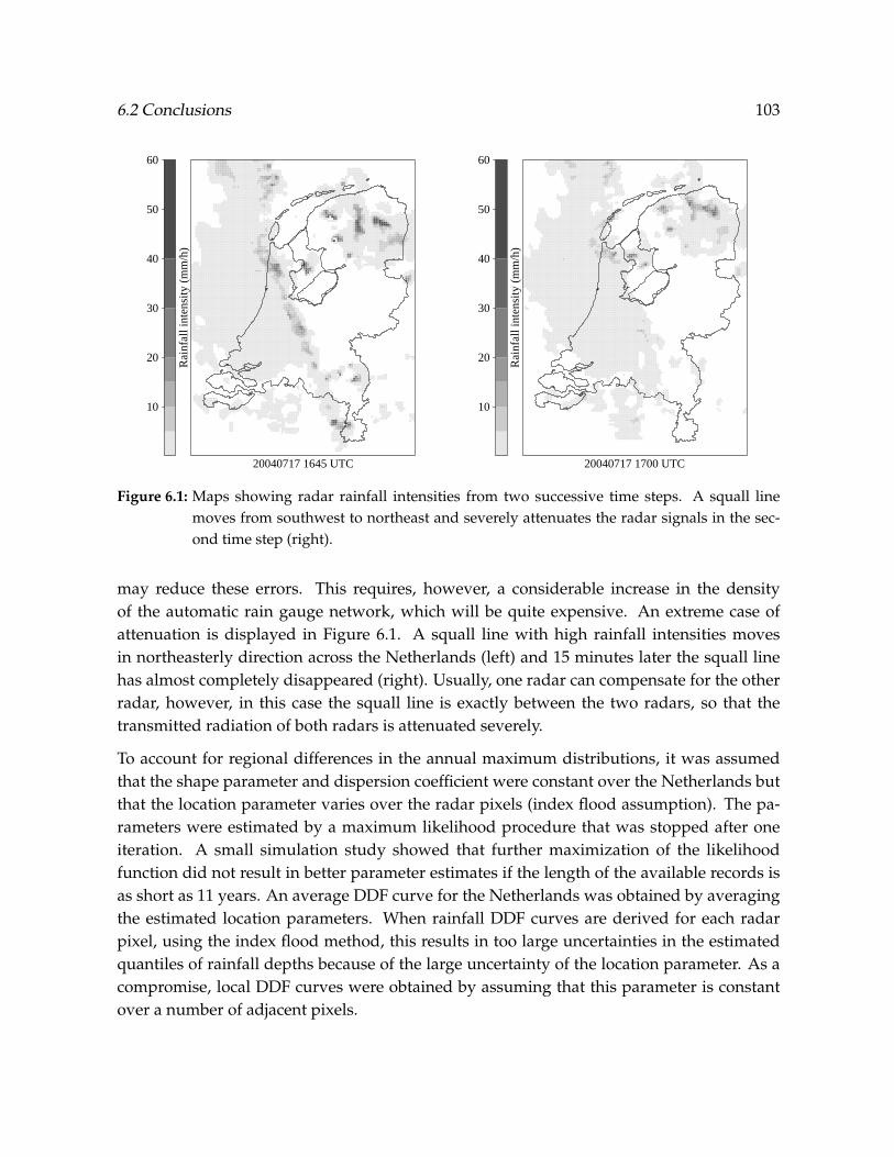
6.2 Conclusions 103
20040717 1645 UTC
Rai
nfal
l int
ensi
ty (
mm
/h)
10
20
30
40
50
60
20040717 1700 UTC
Rai
nfal
l int
ensi
ty (
mm
/h)
10
20
30
40
50
60
Figure 6.1: Maps showing radar rainfall intensities from two successive time steps. A squall line
moves from southwest to northeast and severely attenuates the radar signals in the sec-
ond time step (right).
may reduce these errors. This requires, however, a considerable increase in the density
of the automatic rain gauge network, which will be quite expensive. An extreme case of
attenuation is displayed in Figure 6.1. A squall line with high rainfall intensities moves
in northeasterly direction across the Netherlands (left) and 15 minutes later the squall line
has almost completely disappeared (right). Usually, one radar can compensate for the other
radar, however, in this case the squall line is exactly between the two radars, so that the
transmitted radiation of both radars is attenuated severely.
To account for regional differences in the annual maximum distributions, it was assumed
that the shape parameter and dispersion coefficient were constant over the Netherlands but
that the location parameter varies over the radar pixels (index flood assumption). The pa-
rameters were estimated by a maximum likelihood procedure that was stopped after one
iteration. A small simulation study showed that further maximization of the likelihood
function did not result in better parameter estimates if the length of the available records is
as short as 11 years. An average DDF curve for the Netherlands was obtained by averaging
the estimated location parameters. When rainfall DDF curves are derived for each radar
pixel, using the index flood method, this results in too large uncertainties in the estimated
quantiles of rainfall depths because of the large uncertainty of the location parameter. As a
compromise, local DDF curves were obtained by assuming that this parameter is constant
over a number of adjacent pixels.

104 Chapter 6 — Conclusions and outlook
From 1998 to January 2001, the radar rainfall depths were based on the De Bilt radar only,
because of an elevation bias in the Den Helder data. It is to be expected that incorporating
the Den Helder data will lead to an improved quality of rainfall observations at locations
far from De Bilt, but relatively close to Den Helder. However, it may influence the extreme-
value distributions over a large part of the country. To investigate this, mean-field bias and
spatially (MFBS) adjusted daily and clock-hour rainfall depths were derived based on the De
Bilt radar only (1998-2008). Subsequently, annual maxima were abstracted and the GEV pa-
rameters were estimated. The values of the GEV parameters hardly differ from those based
on the data from the De Bilt (1998-2008) and the Den Helder (2001-2008) radar together. This
also holds for the maps showing the regional differences in the location parameter (Figure
4.9). From this verification it is to be expected that the addition of the Den Helder radar
from 2001 will only have a small influence on the results of the extreme rainfall analysis.
This implies that only one radar is needed to derive a climatology of extreme rainfall within
a radius of 190 km from the radar. This is valid for a flat country and if the radar data are
adjusted using a spatial adjustment on daily rainfall depths (gauge density of 1 per 100 km2)
and a mean-field bias adjustment on hourly rainfall depths (gauge density of 1000 km2).
• Are regional differences in extreme rainfall significant for durations of 15 min to 24 h?
Using 12 automatic rain gauges, in most cases no geographical variation in extreme rainfall
could be found in Chapter 2. This may be attributed to the relatively short period of 29 years,
which causes the uncertainty in the estimated GEV parameters to become rather large, or
to the relatively small number of locations. Significant regional differences in extreme rain-
fall may be found if longer and more digitized time series of rainfall become available for
subdaily durations. Buishand et al. (2009) found significant regional differences in the loca-
tion parameter of the GEV distribution for daily rainfall depths obtained from 141 manual
gauges in the Netherlands, which could only partially be attributed to differences in mean
annual rainfall. Chapter 4 reveals that radar is a promising alternative for studying regional
variability in extreme rainfall. For most durations from 15 min to 24 h, regional variability
in the location parameter in the Netherlands is statistically significant. An important part
of the differences can be attributed to randomness, being relatively large for an 11-year data
set. Nevertheless, patterns of regional differences in the location parameter are comparable
with those obtained from long rain gauge records for 24-h rainfalls (Buishand et al., 2009).
• What is the value of weather radar to obtain areal DDF curves?
A single equation was obtained from which rainfall depths for a chosen return period, and
area size can be calculated for different durations: the areal DDF curve. Areal reduction fac-
tors (ARFs) were also derived. Comparison of these ARFs with those based on rain gauge
data, reveals a good agreement. The ARFs were found to decrease with increasing return pe-
riod, as was also reported by Bell (1976) and Witter (1984). A problem is that the uncertainty
of the shape parameter is very large for large area sizes. This parameter is relevant if long
return periods (> 50 years) are of interest. Another problem is that the effective area the ad-

6.3 Outlook 105
justed radar rainfall depths from a radar pixel are representative of might be smaller than 6
km2, its exact value being unknown. This problem will become less pronounced when radar
data with a 1-km horizontal resolution are available. Further, regional variability in extreme
areal rainfall was not studied. Despite these limitations, the obtained extreme rainfall cli-
matology already has proven to be useful, because the density of rain gauge networks is
usually too low to obtain reliable estimates of extreme areal rainfall for subdaily durations.
• Main conclusion
Only some attempts have been undertaken to obtain extreme rainfall statistics using weather
radar and, specifically, regional variability in extreme rainfall as well as the derivation of
rainfall DDF curves have not been described before. In this thesis a high-quality re-processed
radar data set was obtained, one of the longest described in the literature. Specific attention
was given to the estimation of the uncertainty in rainfall DDF curves. The main result of this
thesis is that weather radar technology has matured and can be used to derive a climatol-
ogy of extreme (areal) rainfall including the uncertainties and can be used to study regional
differences in extreme rainfall. Therefore, it is to be expected that the radar-based extreme
rainfall statistics will gradually replace those derived from rain gauges. Note, however, that
for the time being, rain gauges remain necessary to obtain high-quality radar rainfall depths.
In addition, in some parts of the world weather radars are not operational.
6.3 Outlook
6.3.1 The future of QPE
Chapter 4 showed that extreme radar rainfall depths are smaller than those obtained from
rain gauges for short durations. If long time series of volumetric radar data are available,
these can be used to improve radar rainfall depths, so that they become less prone to changes
in the volumetric profile of reflectivity at short durations. Moreover, although the obtained
climatologies of extreme rainfall based on weather radar are already useful, clearly longer
records are needed to reduce the uncertainty in extreme rainfall depths. An additional 10
years of data would make the derivation of DDF curves for a radar pixel more feasible and
would result in a more reliable study of regional differences in extreme rainfall.
An interesting development is the installation of radars with dual-polarization capability in
several European countries, such as Germany, France and the United Kingdom. Moreover,
the 171 NEXRAD radars covering the United States are being upgraded to dual-polarization
radars the coming years. This type of radar holds a promise for correction for attenuation
and determination of the precipitation type (Bringi and Chandrasekar, 2001). This will lead
to a better discrimination between rain, hail, ground clutter and other spurious echoes, re-
sulting in a better retrieval of rainfall intensities from radar reflectivities. Dual-polarization
radars of the X-band type are specifically suited for urban areas, because of their high spa-
tial resolution, with radar pixels smaller than 1 km2. These radars have a range of typically
50 km and the lower cost per unit compared to radars of the C-band type makes it feasible
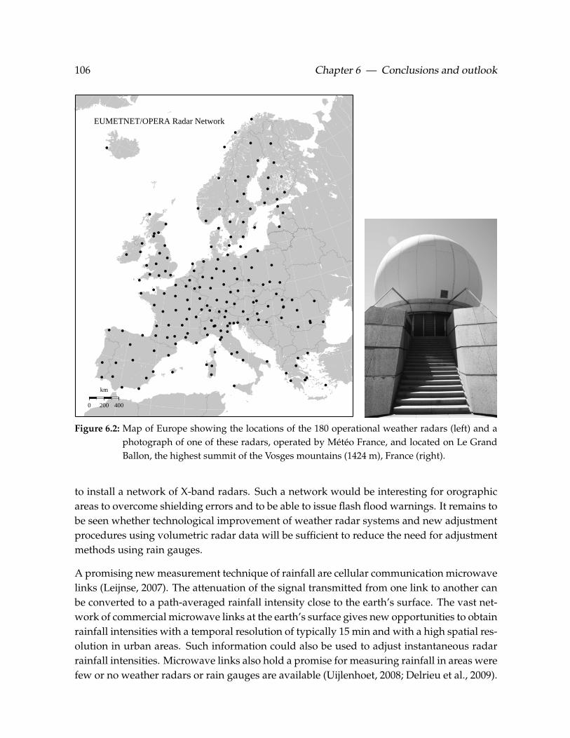
106 Chapter 6 — Conclusions and outlook
0 200 400
km
EUMETNET/OPERA Radar Network
Figure 6.2: Map of Europe showing the locations of the 180 operational weather radars (left) and a
photograph of one of these radars, operated by Meteo France, and located on Le Grand
Ballon, the highest summit of the Vosges mountains (1424 m), France (right).
to install a network of X-band radars. Such a network would be interesting for orographic
areas to overcome shielding errors and to be able to issue flash flood warnings. It remains to
be seen whether technological improvement of weather radar systems and new adjustment
procedures using volumetric radar data will be sufficient to reduce the need for adjustment
methods using rain gauges.
A promising new measurement technique of rainfall are cellular communication microwave
links (Leijnse, 2007). The attenuation of the signal transmitted from one link to another can
be converted to a path-averaged rainfall intensity close to the earth’s surface. The vast net-
work of commercial microwave links at the earth’s surface gives new opportunities to obtain
rainfall intensities with a temporal resolution of typically 15 min and with a high spatial res-
olution in urban areas. Such information could also be used to adjust instantaneous radar
rainfall intensities. Microwave links also hold a promise for measuring rainfall in areas were
few or no weather radars or rain gauges are available (Uijlenhoet, 2008; Delrieu et al., 2009).

6.3 Outlook 107
QPE from satellites is performed using microwave remote sensing techniques, primarily by
employing radiometers to retrieve cloud optical properties and radar. The Tropical Rainfall
Measuring Mission (TRMM) is a successful example of QPE using satellites covering the
globe from 35◦ S to 35◦ N with a revisit time up to several days. The Global Precipitation
Measurement (GPM) Mission is envisaged to perform measurements including the mid-
latitudes with a revisit time of 3 h and a horizontal resolution of 4-5 km and will even be able
to obtain 3-D global precipitation maps with a vertical resolution of 250 m (Uijlenhoet, 2008).
Strangeways (2007) expects that the future of precipitation measurement mainly consists of
combining rain gauge data with satellite data. This will certainly be the case for global
precipitation estimation, since radars are more sparse than rain gauges. However, note that
over large parts of the oceans the only source of precipitation measurements comes from
satellites. In addition, the author of this thesis expects that ground-based weather radars will
become dominant in QPE in the developed countries, which contain many of the world’s
densely populated areas. For the time being, a multi-sensor approach using weather radar
and rain gauges is to be recommended.
The SEVIRI instrument on board of the Meteosat Second Generation (MSG) satellites scans
the complete disk of the earth every 15 minutes. The short revisit time is an advantage over
the TRMM and GPM satellites, however, the MSG does not carry an active precipitation
radar, leading in general to less accurate precipitation estimates. Roebeling and Holleman
(2009) show that rainfall intensities retrieved from MSG during daytime agree reasonably
well with those based on unadjusted weather radar data for an area in the Netherlands.
This holds a promise for using the MSG satellites for QPE during daytime over areas for
which no precipitation observations are available.
The use of radar rainfall data as input for hydrological models is increasing. For example,
Germann et al. (2009) express the uncertainty in radar rainfall depths by creating an ensem-
ble of radar precipitation fields, which are used as input for an hydrological model to obtain
an ensemble of hourly runoff for a 44-km2 Alpine subcatchment. In addition, they show
that runoffs based on deterministic radar data are comparable with those based on gauge
data. Schuurmans and Bierkens (2007) study the influence of spatial variability of daily rain-
fall and hydrological variables on, for instance, discharge using a distributed hydrological
model. They show that operational radar rainfall products are suitable for use in hydrolog-
ical models. Usually only data from one or a few rain gauges are available in a catchment,
which makes radar an interesting alternative.
6.3.2 Applications of climatological radar rainfall data sets
It has been shown that the climatological radar data set, developed in Chapters 3 and 4, has
a high-quality 1. Because the data set has a high temporal and spatial resolution and covers
an entire country, it could also be used:
1The climatological radar data set of 1-hour rainfall depths from Chapter 3 is available at KNMI’s Climate
Services division.

108 Chapter 6 — Conclusions and outlook
• for parameterization of precipitation in weather and climate models
• for verification of the representation of extreme rainfall by climate models
• for verification of precipitation estimates from satellites
• for simulations for satellites which are to be launched
• as input for hydrological or ground water models
• for research on fog formation, air pollution, phenology or traffic density
The presented adjustment methods can be used on radar data sets from other countries
as well. Many meteorological services will operate rain gauge networks with a compara-
ble or higher density. However, for several European countries more difficulties will be
encountered in constructing a high-quality radar data set of rainfall depths. For example,
Nordic countries suffer from errors related to their cold climate (Koistinen et al., 2004) and
in mountainous countries, such as Switzerland, (partial) shielding and ground clutter can be
a severe problem (Germann and Joss, 2004). Further, constructing such long radar data sets
over large areas requires some careful choices to be made, because it is computationally de-
manding, specifically because of the large i/o times due to file processing. Because of this,
the use of long time series of volumetric data provides an additional challenge. Further,
comparison of the quality of climatological radar data sets from the literature is difficult,
because of different climates, the use of other measures of fit and different selection criteria.
Other countries generally exhibit larger spatial differences in extreme rainfall than the Nether-
lands. A computationally more intensive likelihood procedure is then needed to estimate
the parameters of the GEV distribution under the index flood assumption than the one-step
maximization used in Chapter 4. There might be even regional differences in the disper-
sion coefficient and the shape parameter, so that the index flood method is not appropriate
anymore. A possible approach is to link these GEV parameters to mean annual rainfall, see,
e.g., Brath et al. (2003). This may result in rather complex expressions for the DDF curves,
in particular in the case of areal rainfall.
The changing climate could lead to an increase in the severity of extreme rainfall events
(Frei et al., 2006; Lenderink and Van Meijgaard, 2008). Radar holds a promise to frequently
update extreme rainfall statistics for short durations. Ten years of radar data are sufficient
to obtain extreme rainfall statistics with a reasonable accuracy.
In Europe, more than 180 weather radars are operational, covering a large part of the con-
tinent (Figure 6.2). In the framework of the EUMETNET programme OPERA (Holleman
et al., 2008), its European members are working on a new operational data centre where
high-quality composites are derived from radar volume data. This enables the use of radar
data for assimilation in numerical weather prediction models and as input for hydrological

models, which may lead to improved meteorological and hydrological forecasts. In addi-
tion, this opens the way to obtain a long-term radar data set over Europe, which can be em-
ployed to improve our understanding of the climate system (Collier, 1993) and of extreme
rainfall events.
109

110
Bibliography
Ahmad, M. I., C. D. Sinclair, and B. D. Spurr, 1988: Assessment of flood frequency models
using empirical distribution function statistics. Water Resources Research, 24, 1323–1328.
Alila, Y., 1999: A hierarchical approach for the regionalization of precipitation annual max-
ima in Canada. Journal of Geophysical Research, 104 (D24), 31 645–31 655.
Allen, R. J. and A. T. DeGaetano, 2005a: Areal reduction factors for two eastern United
States regions with high rain-gauge density. Journal of Hydrologic Engineering, 10, 327–335,
doi:10.1061/(ASCE)1084–0699(2005)10:4(327).
———, 2005b: Considerations for the use of radar-derived precipitation estimates in deter-
mining return intervals for extreme areal precipitation amounts. Journal of Hydrology, 315,
203–219, doi:10.1016/j.jhydrol.2005.03.028.
Ancona-Navarrete, M. A. and J. A. Tawn, 2002: Diagnostics for pairwise extremal depen-
dence in spatial processes. Extremes, 5, 271–285.
Anderson, T. W. and D. A. Darling, 1952: Asymptotic theory of certain ”goodness of fit”
criteria based on stochastic processes. The Annals of Mathematical Statistics, 23, 193–212.
Atlas, D. and C. W. Ulbrich, 1977: Path- and area-integrated rainfall measurement by mi-
crowave attenuation in the 1-3 cm band. Journal of Applied Meteorology, 16, 1322–1331.
Baeck, M. L. and J. A. Smith, 1995: Climatological analysis of manually digitized radar data
for the United States east of the Rocky Mountains. Water Resources Research, 31, 3033–3049.
Barnes, S. L., 1964: A technique for maximizing details in numerical weather map analysis.
Journal of Applied Meteorology, 3, 396–409.
Bell, F. C., 1976: The Areal Reduction Factor in Rainfall Frequency Estimation. Report no. 35,
Institute of Hydrology, Wallingford.
Borga, M., F. Tonelli, R. J. Moore, and H. Andrieu, 2002: Long-term assessment
of bias adjustment in radar rainfall estimation. Water Resources Research, 38, 1226,
doi:10.1029/2001WR000 555.
111
Borga, M., C. Vezzani, and G. D. Fontana, 2005: Regional rainfall depth-duration-frequency
equations for an Alpine region. Natural Hazards, 36, 221–235.
Brandes, E. A., 1975: Optimizing rainfall estimates with the aid of radar. Journal of Applied
Meteorology, 14, 1339–1345.
Brath, A., A. Castellarin, and A. Montanari, 2003: Assessing the reliability of regional depth-
duration-frequency equations for gaged and ungaged sites. Water Resources Research, 39,
1367, doi:10.1029/2003WR002 399.
Bringi, V. N. and V. Chandrasekar, 2001: Polarimetric Doppler Weather Radar: Principles and
Applications. Cambridge University Press, Cambridge.
Buishand, T. A., 1984: Bivariate extreme-value data and the station-year method. Journal of
Hydrology, 69, 77–95.
———, 1989: Statistics of extremes in climatology. Statistica Neerlandica, 43, 1–30,
doi:10.1111/j.1467–9574.1989.tb01 244.x.
———, 1991: Extreme rainfall estimation by combining data from several sites. Hydrological
Sciences Journal, 36, 345–365.
———, 1993: Rainfall depth-duration-frequency curves; a problem of dependent extremes.
Statistics for the Environment, Barnett, V. and K. F. Turkman, Eds., Wiley, Chichester, 183–
197.
Buishand, T. A., L. De Haan, and C. Zhou, 2008: On spatial extremes: with application to a
rainfall problem. The Annals of Applied Statistics, 2, 624–642, doi:10.1214/08–AOAS159.
Buishand, T. A., R. Jilderda, and J. B. Wijngaard, 2009: Regionale verschillen
in extreme neerslag. Scientific report WR-2009-01, KNMI, De Bilt, available via
www.knmi.nl/bibliotheek/knmipubWR/WR2009-01.pdf (in Dutch).
Buishand, T. A., J. B. M. Van Acker, and H. Van Luijtelaar, 1991: Analyse van kwartiersom-
men van de neerslag. H2O, 24, 294–299 (in Dutch).
Buishand, T. A. and C. A. Velds, 1980: Neerslag en Verdamping. KNMI, De Bilt (in Dutch).
Buishand, T. A. and J. B. Wijngaard, 2007: Statistiek van extreme neerslag voor
korte neerslagduren. Technical report TR-295, KNMI, De Bilt, available via
www.knmi.nl/publications/fulltexts/tr295.pdf (in Dutch).
Burn, D. H., 2003: The use of resampling for estimating confidence intervals for single site
and pooled frequency analysis. Hydrological Sciences Journal, 48, 25–38.
112

Carbone, R. and J. D. Tuttle, 2008: Rainfall occurrence in the U.S. warm season: the diurnal
cycle. Journal of Climate, 21, 4132–4146, doi:10.1175/2008JCLI2275.1.
Ciach, G. J. and W. F. Krajewski, 1999: On the estimation of radar rainfall error variance.
Advances in Water Resources, 22, 585–595.
———, 2006: Analysis and modeling of spatial correlation structure in small-
scale rainfall in Central Oklahoma. Advances in Water Resources, 29, 1450–1463,
doi:10.1016/j.advwatres.2005.11.003.
Cleveland, W. S., 1979: Robust locally weighted regression and smoothing scatterplots. Jour-
nal of the American Statistical Association, 74, 829–836.
Coles, S., 2001: An Introduction to Statistical Modeling of Extreme Values. Springer, London.
Coles, S. G., 1993: Regional modelling of extreme storms via max-stable processes. Journal of
the Royal Statistical Society, Series B, 55, 797–816.
Coles, S. G. and M. J. Dixon, 1999: Likelihood-based inference for extreme value models.
Extremes, 2, 5–23.
Coles, S. G. and J. A. Tawn, 1996: Modelling extremes of the areal rainfall process. Journal of
the Royal Statistical Society, Series B, 58, 329–347.
Collier, C. G., 1989: Applications of Weather Radar Systems: a Guide to Uses of Radar Data in
Meteorology and Hydrology. Ellis Horwood Limited, Chichester, England.
———, 1993: The application of a continental-scale radar database to hydrological process
parametrization within Atmospheric General Circulation Models. Journal of Hydrology,
142, 301–318.
Croft, P. J. and M. D. Shulman, 1989: A five-year radar climatology of convective precipita-
tion for New Jersey. International Journal of Climatology, 9, 581–600.
Dekker, A., H. Van Gasteren, W. Bouten, J. Shamoun-Baranes, A. Borst, I. Holleman, A. Dok-
ter, A. Ginati, and G. Garofalo, 2008: The European Space Agency’s Flysafe project, look-
ing at the bird strike problem from another perspective. Proceedings of the 28th meeting of
the International Bird Strike Committee, International Bird Strike Committee, s.l., available
via http://dare.uva.nl/record/295060.
Delbeke, L., 2000: Extreme Neerslag in Vlaanderen; nieuwe IDF-curven gebaseerd op langdurige
meetreeksen van neerslag. Koninklijk Meteorologisch Instituut, Ukkel (in Dutch).
Delrieu, G., I. Braud, A. Berne, M. Borga, B. Boudevillain, F. Fabry, J. Freer, E. Gaume,
E. Nakakita, A. Seed, P. Tabary, and R. Uijlenhoet, 2009: Weather radar and hydrology.
Advances in Water Resources, 32, 969–974, doi:10.1016/j.advwatres.2009.03.006.
113

Diaconis, P. and B. Efron, 1983: Computer-intensive methods in statistics. Scientific American,
248, 96 – 108.
Doviak, R. J. and D. S. Zrnic, 1993: Doppler Radar and Weather Observations. 2d ed., Dover
Publications, Inc., Mineola, New York.
Durrans, S. R., L. T. Julian, and M. Yekta, 2002: Estimation of depth-area rela-
tionships using radar-rainfall data. Journal of Hydrologic Engineering, 7, 356 – 367,
doi:10.1061/(ASCE)1084–0699(2002)7:5(356).
Efron, B. and R. J. Tibshirani, 1993: An Introduction to the Bootstrap. Chapman & Hall, New
York.
Faulkner, D. S. and D. A. Jones, 1999: The FORGEX method of rainfall growth estimation III:
Examples and confidence intervals. Hydrology and Earth System Sciences, 3, 205–212.
Figueras i Ventura, J. and H. W. J. Russchenberg, 2009: Towards a better understanding of the
impact of anthropogenic aerosols in the hydrological cycle: IDRA, IRCTR drizzle radar.
Physics and Chemistry of the Earth, Parts A/B/C, 34, 88–92, doi:10.1016/j.pce.2008.02.038.
Fowler, H. J. and C. G. Kilsby, 2003: A regional frequency analysis of United Kingdom ex-
treme rainfall from 1961 to 2000. International Journal of Climatology, 23, 1313–1334.
Frederick, R. H., V. A. Myers, and E. P. Auciello, 1977: Storm depth-area relations from
digitized radar returns. Water Resources Research, 13, 675–679.
Frei, C., R. Scholl, S. Fukutome, J. Schmidli, and P. Vidale, 2006: Future change of precip-
itation extremes in Europe: Intercomparison of scenarios from regional climate models.
Journal of Geophysical Research, 111, D06 105.
Gabella, M., J. Joss, G. Perona, and G. Galli, 2001: Accuracy of rainfall estimates by two
radars in the same Alpine environment using gage adjustment. Journal of Geophysical Re-
search, 106(D6), 5139–5150.
Gellens, D., 2002: Combining regional approach and data extension procedure for assessing
GEV distribution of extreme precipitation in Belgium. Journal of Hydrology, 268, 113–126.
———, 2003: Etude des precipitations extremes: Etablissement des fractiles et des periodes de retour
d’evenements pluviometriques. These de doctorat. Universite Libre de Bruxelles (in French).
Germann, U., M. Berenguer, D. Sempere-Torres, and M. Zappa, 2009: REAL - Ensemble
radar precipitation estimation for hydrology in a mountainous region. Quarterly Journal of
the Royal Meteorological Society, 135, 445–456, doi:10.1002/qj.375.
114

Germann, U., G. Galli, M. Boscacci, and M. Bolliger, 2006: Radar precipitation measurement
in a mountainous region. Quarterly Journal of the Royal Meteorological Society, 132, 1669–
1692, doi:10.1256/qj.05.190.
Germann, U. and J. Joss, 2002: Mesobeta profiles to extrapolate radar precipitation measure-
ments above the Alps to the ground level. Journal of Applied Meteorology, 41, 542–557.
———, 2004: Operational measurement of precipitation in mountainous terrain. Weather
Radar: Principles and Advanced Applications, Meischner, P., Ed., Springer-Verlag, Berlin Hei-
delberg, 52–77.
GREHYS, 1996: Inter-comparison of regional flood frequency procedures for Canadian
rivers. Journal of Hydrology, 186, 85–103.
Gringorten, I. I., 1963: A plotting rule for extreme probability paper. Journal of Geophysical
Research, 68, 813–814.
Hand, W. H., 1996: An object-oriented technique for nowcasting heavy showers and thun-
derstorms. Meteorological Applications, 3, 31–41.
Hershfield, D. M., 1961: Rainfall Frequency Atlas of the United States: For Durations from 30
Minutes to 24 Hours and Return Periods from 1 to 100 Years. Technical Paper No. 40, U.S.
Department of Commerce, Weather Bureau, Washington D.C.
Holleman, I., 2007: Bias adjustment and long-term verification of radar-based precipitation
estimates. Meteorological Applications, 14, 195–203, doi:10.1002/met.22.
Holleman, I. and H. Beekhuis, 2005: Review of the KNMI Clutter Removal Scheme. Technical
report TR-284, KNMI, De Bilt, available via
http://www.knmi.nl/publications/fulltexts/tr clutter.pdf.
Holleman, I., L. Delobbe, and A. Zgonc, 2008: Update on the European weather radar net-
work (opera). Fifth European Conference on Radar in Meteorology and Hydrology, 30 June - 4
July 2008, Helsinki, Finland.
Hosking, J. R. M. and J. R. Wallis, 1997: Regional Frequency Analysis: an Approach Based on
L-moments. Cambridge University Press, Cambridge.
Hosking, J. R. M., J. R. Wallis, and E. F. Wood, 1985: Estimation of the generalized extreme-
value distribution by the method of probability-weighted moments. Technometrics, 27,
251–261.
Jenkinson, A. F., 1955: The frequency distribution of the annual maximum (or minimum)
values of meteorological elements. Quarterly Journal of the Royal Meteorological Society, 81,
158–171.
115

Joss, J. and R. Lee, 1995: The application of radar-gauge comparisons to operational precip-
itation profile corrections. Journal of Applied Meteorology, 34, 2612–2630.
Joss, J. and A. Waldvogel, 1990: Precipitation measurement and hydrology. Radar in Meteo-
rology, Battan, L. J. and D. Atlas, Eds., American Meteorological Society, Boston, 577–606.
Kitchen, M. and R. M. Blackall, 1992: Representativeness errors in comparisons between
radar and gauge measurements of rainfall. Journal of Hydrology, 134, 13–33.
KNMI, 2000: Handbook for the Meteorological Observation. KNMI, 91-110 pp., available via
http://www.knmi.nl/samenw/hawa/download.html.
Koistinen, J., D. B. Michelson, H. Hohti, and M. Peura, 2004: Operational measurement of
precipitation in cold climates. Weather Radar: Principles and Advanced Applications, Meis-
chner, P., Ed., Springer-Verlag, Berlin Heidelberg, 78–114.
Koistinen, J., H. Pohjola, and H. Hohti, 2003: Vertical reflectivity profile classification and
correction in radar composites in Finland. 31st Conference on Radar Meteorology (Volume I),
American Meteorological Society, Boston, 534–537.
Koistinen, J. and T. Puhakka, 1981: An improved spatial gauge-radar adjustment technique.
Twentieth Conference on Radar Meteorology, American Meteorological Society, Boston, 179–
186, available via http://ams.confex.com/ams/pdfpapers/64 306.pdf.
Kok, C. J., B. G. J. W. Schreur, and D. H. P. Vogelezang, 2009: Meteorological support for
anticipatory water management. Atmospheric Research, submitted.
Koutsoyiannis, D., 2004: Statistics of extremes and estimation of extreme rainfall: II. Empir-
ical investigation of long rainfall records. Hydrological Sciences Journal, 49, 591–610.
Koutsoyiannis, D. and G. Baloutsos, 2000: Analysis of a long record of annual maximum
rainfall in Athens, Greece, and design rainfall inferences. Natural Hazards, 29, 29–48.
Koutsoyiannis, D., D. Kozonis, and A. Manetas, 1998: A mathematical framework for study-
ing rainfall intensity-duration-frequency relationships. Journal of Hydrology, 206, 118–135.
Kysely, J. and J. Picek, 2007: Regional growth curves and improved design value estimates
of extreme precipitation events in the Czech Republic. Climate Research, 33, 243–255.
Leijnse, H., 2007: Hydrometeorological Application of Microwave Links: Measurement of Evapo-
ration and Precipitation. PhD dissertation, Wageningen University, Wageningen, available
via http://library.wur.nl/wda/dissertations/dis4353.pdf.
Lenderink, G. and E. Van Meijgaard, 2008: Increase in hourly precipitation extremes
beyond expectations from temperature changes. Nature Geoscience, 1, 511 – 514,
doi:10.1038/ngeo262.
116

Lombardo, F., F. Napolitano, and F. Russo, 2006: On the use of radar reflectivity for estima-
tion of the areal reduction factor. Natural Hazards and Earth System Sciences, 6, 377–386.
Madsen, H., P. S. Mikkelsen, D. Rosbjerg, and P. Harremoes, 2002: Regional esti-
mation of rainfall intensity-duration-frequency curves using generalized least squares
regression of partial duration series statistics. Water Resources Research, 38, 1239,
doi:10.1029/2001WR001 125.
Madsen, H., C. P. Pearson, and D. Rosbjerg, 1997a: Comparison of annual maximum series
and partial duration series methods for modeling extreme hydrologic events. 2. Regional
modeling. Water Resources Research, 33, 759–769.
Madsen, H., P. F. Rasmussen, and D. Rosbjerg, 1997b: Comparison of annual maximum
series and partial duration series methods for modeling extreme hydrologic events. 1. At-
site modeling. Water Resources Research, 33, 747–757.
Marshall, J. S., W. Hitschfeld, and K. L. S. Gunn, 1955: Advances in radar weather. Advances
in Geophysics, Academic Press, New York, Vol. 2, 1–56.
Marshall, J. S. and W. M. Palmer, 1948: The distribution of raindrops with size. Journal of the
Atmospheric Sciences, 5, 165–166.
Martins, E. S. and J. R. Stedinger, 2000: Generalized maximum-likelihood generalized
extreme-value quantile estimators for hydrologic data. Water Resources Research, 36, 737–
744.
Menabde, M., A. Seed, and G. Pegram, 1999: A simple scaling model for extreme rainfall.
Water Resources Research, 35, 335–339.
Michelson, D., T. Einfalt, I. Holleman, U. Gjertsen, K. Friedrich, G. Haase, M. Lindskog, and
A. Jurczyk, (Eds.) , 2005a: COST Action 717: Weather Radar Data Quality in Europe: Quality
Control and Characterisation - Review. EU Publications Office (Brussels), EUR 21955.
Michelson, D. B., C. G. Jones, T. Landelius, C. G. Collier, G. Haase, and M. Heen,
2005b: ‘Down-to-Earth’ modelling of equivalent surface precipitation using multisource
data and radar. Quarterly Journal of the Royal Meteorological Society, 131, 1093–1112,
doi:10.1256/qj.03.203.
Michelson, D. B. and J. Koistinen, 2000: Gauge-radar network adjustment for the Baltic Sea
Experiment. Physics and Chemistry of the Earth, Part B: Hydrology, Oceans and Atmosphere,
25, 915–920.
Mora, R. D., C. Bouvier, L. Neppel, and H. Niel, 2005: Regional approach for the estimation
of low-frequency distribution of daily rainfall in the Languedoc-Roussillon region, France.
Hydrological Sciences Journal, 50, 17–29 (in French).
117

Morrison, J. E. and J. A. Smith, 2002: Stochastic modeling of flood peaks us-
ing the generalized extreme value distribution. Water Resources Research, 38, 1305,
doi:10.1029/2001WR000 502.
Nelson, B. R., W. F. Krajewski, A. Kruger, J. A. Smith, and M. L. Baeck, 2003: Archival
precipitation data set for the Mississippi River Basin: Algorithm development. Journal of
Geophysical Research, 108, No. D22, 8857, doi:10.1029/2002JD003 158.
NERC, 1975: Flood Studies Report. Natural Environment Research Council, London.
Nicol, J. C. and G. L. Austin, 2003: Attenuation correction constraint for single-polarisation
weather radar. Meteorological Applications, 10, 345–354, doi:10.1017/S1350482703001 051.
Northrop, P. J., 2004: Likelihood-based approaches to flood frequency estimation. Journal of
Hydrology, 292, 96 – 113, doi:10.1016/j.jhydrol.2003.12.031.
Nzeukou, A., H. Sauvageot, and L. Feral, 2006: Rain rate and attenuation statistics
along paths in a tropical coastal area from radar data. Radio Science, 41, RS2005,
doi:10.1029/2004RS003 227.
Omolayo, A. S., 1993: On the transposition of areal reduction factors for rainfall frequency
estimation. Journal of Hydrology, 145, 191–205.
Press, W. H., S. A. Teukolsky, W. T. Vetterling, and B. P. Flannery, 1992: Numerical Recipes in
C: The Art of Scientific Computing. 2d ed., Cambridge University Press.
Probert-Jones, J. R., 1962: The radar equation in meteorology. Quarterly Journal of the Royal
Meteorological Society, 88, 485–495.
Raghavan, S., 2003: Radar Meteorology. Kluwer Academic Publishers.
Reed, D. W., D. S. Faulkner, and E. J. Stewart, 1999: The FORGEX method of rainfall growth
estimation II: Description. Hydrology and Earth System Sciences, 3, 197–203.
Rinehart, R. E., 2004: Radar for Meteorologists. 4th ed., Rinehart Publications.
Roebeling, R. and I. Holleman, 2009: SEVIRI rainfall retrieval and validation using
weather radar observations. Journal of Geophysical Research (Atmospheres), in press,
doi:10.1029/2009JD012 102.
Rosenfeld, D. and E. Amitai, 1998: Comparison of WPMM versus regression for evaluating
Z-R relationships. Journal of Applied Meteorology, 37, 1241–1249.
Rosenfeld, D., D. B. Wolff, and D. Atlas, 1993: General probability-matched relations be-
tween radar reflectivity and rain rate. Journal of Applied Meteorology, 32, 50–72.
118

Schaefer, M. G., 1990: Regional analyses of precipitation annual maxima in Washington
State. Water Resources Research, 26, 119–131.
Schuurmans, J. M. and M. F. P. Bierkens, 2007: Effect of spatial distribution of daily rainfall
on interior catchment response of a distributed hydrological model. Hydrology and Earth
System Sciences, 11, 677–693.
Smith, W. H. F. and P. Wessel, 1990: Gridding with continuous curvature splines in tension.
Geophysics, 55, 293–305.
Smits, I., J. B. Wijngaard, R. P. Versteeg, and M. Kok, 2004: Statistiek van extreme neerslag in
Nederland. STOWA publicatie 2004-26, STOWA, Utrecht (in Dutch).
Stedinger, J. R. and G. D. Tasker, 1985: Regional hydrologic analysis 1. Ordinary, weighted,
and generalized least squares compared. Water Resources Research, 21, 1421–1432.
Steiner, M., J. A. Smith, S. J. Burges, C. V. Alonso, and R. W. Darden, 1999: Effect of bias ad-
justment and rain gauge data quality control on radar rainfall estimation. Water Resources
Research, 35, 2487–2503.
Stewart, E. J., D. W. Reed, D. S. Faulkner, and N. S. Reynard, 1999: The FORGEX method of
rainfall growth estimation I: Review of requirement. Hydrology and Earth System Sciences,
3, 187–195.
Strangeways, I., 2007: Precipitation: Theory, Measurement and Distribution. Cambridge Uni-
versity Press, Cambridge.
Sveinsson, O. G. B., D. C. Boes, and J. D. Salas, 2001: Population index flood method for
regional frequency analysis. Water Resources Research, 37, 2733–2748.
Uijlenhoet, R., 2008: Precipitation physics and rainfall observation. Climate and the Hydrologi-
cal Cycle, Bierkens, M. F. P., A. J. Dolman, and P. A. Troch, Eds., IAHS Special Publication 8,
International Association of Hydrological Sciences, Wallingford, 59–97.
Uijlenhoet, R. and J. N. M. Stricker, 1999: A consistent rainfall parameterization based on
the exponential raindrop size distribution. Journal of Hydrology, 218, 101–127.
U.S. Weather Bureau, 1964: Two- to ten-day Precipitation for Return Periods of 2 to 100 Years
in the Contiguous United States. Technical Paper No. 49, U.S. Department of Commerce,
Weather Bureau, Washington D.C.
Van Luijtelaar, H., 2006: Stedelijke wateropgave: Vergelijking normen voor
water op straat en inundatie. Stichting RIONED, Ede, available via
http://www.riool.net/riool/shopping/products/overview.do (in Dutch).
119

Van Montfort, M. A. J. and J. V. Witter, 1986: The Generalized Pareto distribution applied to
rainfall depths. Hydrological Sciences Journal, 31, 151–162.
Vignal, B., G. Galli, J. Joss, and U. Germann, 2000: Three methods to determine profiles of
reflectivity from volumetric radar data to correct precipitation estimates. Journal of Applied
Meteorology, 39, 1715–1726.
Vignal, B. and W. F. Krajewski, 2001: Large-sample evaluation of two methods to correct
range-dependent error for WSR-88D rainfall estimates. Journal of Hydrometeorology, 2, 490–
504.
Wauben, W., 2006: KNMI Contribution to the WMO Laboratory Intercomparison of
Rainfall Intensity Gauges. Technical report TR-287, KNMI, De Bilt, available via
http://www.knmi.nl/˜wauben.
Wessels, H. R. A. and J. H. Beekhuis, 1995: Stepwise procedure for suppression of anoma-
lous ground clutter. COST 75 Weather Radar Systems, International Seminar, EUR 16013 EN,
Luxembourg, 270–277.
Willems, P., 2000: Compound intensity/duration/frequency-relationships of extreme pre-
cipitation for two seasons and two storm types. Journal of Hydrology, 233, 189–205.
Witter, J. V., 1984: Heterogeneity of Dutch rainfall. PhD dissertation, Wageningen University,
Wageningen.
WMO, 1981: Guide to Hydrological Practices, Volume I - Data Acquisition and Processing. WMO-
No. 168, Section 4.2.1.2.2.
Xie, H., X. Zhou, J. M. H. Hendrickx, E. R. Vivoni, H. Guan, Y. Q. Tian, and E. E. Small, 2006:
Evaluation of NEXRAD stage III precipitation data over a semiarid region. Journal of the
American Water Resources Association, 42, 237–256.
Young, C. B., A. A. Bradley, W. F. Krajewski, and A. Kruger, 2000: Evaluating NEXRAD
multisensor precipitation estimates for operational hydrologic forecasting. Journal of Hy-
drometeorology, 1, 241–254.
Zondervan, J. G., 1978: Modelling Urban Run-off; a Quasilinear Approach. PhD dissertation,
Centre for Agricultural Publishing and Documentation, Wageningen.
Zucchini, W. and P. T. Adamson, 1989: Bootstrap confidence intervals for design storms from
exceedance series. Hydrological Sciences Journal, 34, 41–48.
120

Appendix A
Bootstrap algorithm for estimating
standard deviations and correlation
coefficients of estimated GEV parameters
The bootstrap is applied to the running and sliding annual maximum rainfalls. Because the
sliding annual maxima are only available for De Bilt, the annual maxima from De Bilt and
the other stations are sampled separately. The two bootstrap samples are then concatenated
to form a bootstrap sample of 514 years with the same layout as the original sample of
annual maximum rainfalls. This procedure is similar to the regional bootstrap in GREHYS
(1996). A precise description of the bootstrap algorithm is presented below. Steps 3 and 4
are illustrated in Table A.1.
1. Split the annual maxima series of 514 years into a series of 84 years with year numbers
1, 2, .., 84, belonging to De Bilt 1906-1990, and a series of 430 years with year numbers
85, 86, .., 514.
2. Draw for each of the two series of year numbers a random sample with replacement
(bootstrap sample).
3. Select the running annual maxima for the sampled year numbers for D = 1, 2, 4, 8, 12,
24 h. This leads to one bootstrap sample of 84 years of running annual maxima and
one bootstrap sample of 430 years of running annual maxima for each D. For D = 1,
2 h also a bootstrap sample of 84 sliding annual maxima is constructed using the same
year numbers as for the 84 running annual maxima.
4. Construct bootstrap samples of 514 years by adding the 84-year to the 430-year run-
ning annual maxima.
121

122 Appendix A — Bootstrap algorithm
5. Fit a GEV distribution to the bootstrap sample of 514 years for each of the durations of
1, 2, 4, 8, 12 and 24 h.
6. Fit a GEV distribution to the bootstrap sample of 84 years for durations of 1 and 2 h
individually. Do this separately for the bootstrap samples of running and sliding max-
ima.
7. Apply Eqs. (2.18)-(2.20) for D = 1, 2 h.
8. Repeat this 104 times, so that 104 bootstrap samples are drawn and 104 GEV parameters
are estimated for each duration.
9. Determine the standard deviation of each estimated GEV parameter as the sample
standard deviation of that parameter estimate in the 104 bootstrap samples.
10. Determine the correlation between estimated GEV parameters by calculating the cor-
relation between these parameter estimates in the 104 bootstrap samples.
Table A.1: Application of the bootstrap.
Year
number
Running
annual
maximum
(mm)
Sliding annual
maximum
(mm)
Drawn bootstrap
samples
1 13.2 17.3 | 84 running
2 9.2 9.2 | and 84 sliding
. .. .. | maxima
84 9.1 10.0 | De Bilt
85 17.4 not available | 430
86 15.3 not available | running
. .. not available | maxima
514 16.9 not available |
514 running maxima+
Appendix B
Maximum likelihood versus L-moments
A number of simulation experiments have been conducted by Sveinsson et al. (2001) to
compare maximum likelihood estimation with L-moments methods under the index flood
assumption. These experiments were restricted to a small number of sites. This appendix
discusses a simulation experiment in which there are 200 sites, each having a record of only
11 annual maxima. It is assumed that the 200 × 11 annual maxima are independent. The
maxima are generated from a GEV distribution with γ = 0.245 and κ = -0.170. The average
µ is 34.75 mm: for 160 sites a 5% smaller value and for 40 sites a 20% larger value of µ is used
in the simulation, which roughly corresponds to the regional differences of µ for D = 24 h
in the Netherlands. The simulations are repeated 600 times.
Two L-moments methods and three maximum likelihood methods are considered. The first
L-moments method is that used in the UK Flood Estimation Handbook (FEH) as described
by Fowler and Kilsby (2003). For each site annual maxima are scaled with their median
value and the L-moments ratios L-CV and L-SKEW are calculated. Subsequently, these L-
moments ratios from the 200 sites are averaged and the GEV parameters are estimated from
the average L-moments ratios and the at-site median. In the second L-moments method
the average is used as the index flood instead of the median (Hosking and Wallis, 1997).
The maximum likelihood procedure used in Chapter 4, in which the iteration is stopped
after one step, is compared with two alternatives, the full maximization of the likelihood
under the index flood assumption and the full maximization with only two regional location
parameters. In the latter case one value of µ is estimated for the 40 sites with a relatively large
value of this parameter and one value for the other 160 sites.
For the five estimation procedures, Table B.1 shows the means of the estimated GEV param-
eters, and the resulting 50-year rainfall depth, x(50), in the 600 simulations. The estimates of
the location parameter and the 50-year rainfall depth have been averaged over the 200 sites.
The standard deviations of the estimated GEV parameters and x(50) were also derived from
123

124 Appendix B — Maximum likelihood versus L-moments
the 600 simulations.
The table shows that both L-moments methods result in a large bias of κ. Though the stan-
dard errors of the L-moments estimates of µ, γ and κ are generally larger than those of the
maximum likelihood estimates, this does not lead to a larger standard error of x(50). Some-
thing similar was also observed by Morrison and Smith (2002) who compared L-moments
estimates with mixed maximum likelihood L-moments estimates. The one-step maximum
likelihood procedure results in a somewhat larger bias in γ than the L-moments methods,
but there is no bias in κ. The full maximum likelihood procedure under the index flood
assumption does not provide better estimates. In particular, it leads to a considerable bias
of κ and an increase of the standard error of this parameter estimate. Obviously, the large
uncertainty of the 200 at-site estimates of µ deteriorates the quality of the estimate of the
common κ. Similar results were obtained in the case of 500 sites. Full maximization with
two regional values of µ gives almost unbiased estimates of the common parameters. In this
case the standard errors of the estimated location parameters are much smaller than those
for the index flood method (not shown in Table B.1).
The bottom rows of Table B.1 give the results for a simulation experiment in which the num-
ber of annual maxima was increased to 50 per site. For this sample size the full maximum
Table B.1: Means and standard deviations (between brackets) of estimated GEV parameters and es-
timated 50-year rainfall depth x(50) in two simulation experiments. FEH indicates the
method used in the UK Flood Estimation Handbook and HW refers to the method em-
ployed in Hosking and Wallis (1997), and ML stands for maximum likelihood.
Method µ (mm) γ κ x(50) (mm)
True values 34.75 0.245 -0.170 81.9
Regional variability, 11 annual maxima
L-moments (FEH) 35.05 (0.24) 0.255 (0.005) -0.113 (0.019) 78.7 (1.7)
L-moments (HW) 35.10 (0.22) 0.255 (0.005) -0.113 (0.019) 78.8 (1.7)
ML, one step 35.31 (0.20) 0.260 (0.004) -0.170 (0.017) 86.0 (2.1)
Full ML, index flood 34.84 (0.22) 0.228 (0.004) -0.205 (0.025) 82.4 (2.3)
Full ML, regional µ 34.77 (0.21) 0.245 (0.004) -0.167 (0.017) 81.7 (1.8)
Regional variability, 50 annual maxima
L-moments (FEH) 34.81 (0.11) 0.247 (0.002) -0.156 (0.009) 81.1 (0.9)
L-moments (HW) 34.83 (0.10) 0.247 (0.002) -0.156 (0.009) 81.1 (0.9)
ML, one step 35.01 (0.10) 0.260 (0.002) -0.170 (0.008) 85.5 (1.0)
Full ML, index flood 34.78 (0.10) 0.242 (0.002) -0.174 (0.008) 81.8 (0.9)
Full ML, regional µ 34.75 (0.10) 0.245 (0.002) -0.169 (0.008) 81.8 (0.9)

125
likelihood method under the index flood assumption performs well. In particular, the biases
are smaller than in the case of L-moments estimation and the one-step maximum likelihood
estimation. There is no longer a deteriorating effect of the estimated at-site location param-
eters on the estimates of the common dispersion coefficient and shape parameter.
Sveinsson et al. (2001) presented a number of alternative L-moments methods resulting in
less bias of a large quantile of the distribution than the L-moments methods considered here,
however, at the cost of an increase in the standard deviation of the estimated quantile.
The one-step maximum likelihood procedure breaks down if the regional differences in the
location parameter are larger than in the Netherlands. A full maximization of the likelihood
(with some regionalization of the location parameter in the case of very short records) is
then needed, which is computationally more demanding.

126 Appendix B — Maximum likelihood versus L-moments

Appendix C
Influence of missing data on estimated
GEV parameters
As was noted in Section 4.4, the average radar data availability is approximately 90% in
the period where most annual maxima occur. A part of the observed annual maximum
rainfall depths will therefore be lower than the true annual maxima, which influences the
parameters of the GEV distribution. This influence is quantified here theoretically for the
case of a negative shape parameter κ.
The GEV distribution for annual maxima is related to the Generalized Pareto Distribution
(GPD), which describes the distribution of the exceedances Y = X − u of a high threshold u
in the associated peak-over-threshold model. The cumulative distribution of Y is given by:
H(y) = 1 −(
1 −κy
σ
)1/κfor κ 6= 0. (C.1)
The number of exceedances of the threshold u in a year follows a Poisson distribution with
mean λ(u). The GEV parameters µ and α are related to λ(u) and the GPD parameters σ
and κ (Buishand, 1989; Madsen et al., 1997b):
µ = u + σ[1 − λ−κ(u)]/κ for κ 6= 0, (C.2)
α = σ/λκ(u). (C.3)
The value of the GEV parameter κ is equal to the value of the GPD parameter κ. In case
a fraction f of the exceedances is missing, the Poisson distribution still holds if the missing
exceedances are randomly distributed in time. The average number of exceedances in a year
then becomes λ∗(u) = (1 − f )λ(u). Using this expression and Eq. (C.3), the new value of α
becomes:
α∗ = (1 − f )−κα. (C.4)
127

Due to the change of λ(u), Eq. (C.2) changes into
µ∗ = u + σ[1 − (1 − f )−κλ−κ(u)]/κ for κ 6= 0. (C.5)
Now, Eq. (C.2) is substracted from Eq. (C.5), which results in:
µ∗ = µ +α
κ[1 − (1 − f )−κ] for κ 6= 0, (C.6)
using Eq. (C.3). The new value of the dispersion coefficient is given by:
γ∗ =α∗
µ∗=
(1 − f )−κ
1 + γ[1 − (1 − f )−κ]/κγ for κ 6= 0. (C.7)
Eqs. (C.6) and (C.7) are used to estimate the change in µ and γ in case f = 0.1, which
corresponds to a data availability of 90%. Note that the relative changes in these parameters
only depend on γ and κ. For γ = 0.245 and κ = -0.170, representative of annual maximum
precipitation for D = 24 h, µ∗ is 2.6% smaller than µ and γ∗ increases 0.8% with respect to γ.
For D = 15 min, realistic values of γ and κ are respectively 0.346 and -0.110 and µ∗ decreases
3.6% with respect to µ and for γ∗ an increase of 2.6% is found. This demonstrates that 10%
missing data has little influence on the value of the estimated GEV parameters.
128

List of Publications
Peer-reviewed articles
Van Vliet A.J.H., A. Overeem, R.S. De Groot, A.F.G. Jacobs, and F.T.M. Spieksma, 2002: The influence
of temperature and climate change on the timing of pollen release in the Netherlands. International
Journal of Climatology, 22, 1757-1767, doi:10.1002/joc.820.
Overeem, A., A. Buishand, and I. Holleman, 2008: Rainfall depth-duration-frequency curves and
their uncertainties. Journal of Hydrology, 348, 124-134, doi:10.1016/j.jhydrol.2007.09.044.
Overeem, A., I. Holleman, and A. Buishand, 2009: Derivation of a 10-year radar-based climatology of
rainfall. Journal of Applied Meteorology and Climatology, 48, 1448-1463, doi:10.1175/2009JAMC1954.1.
Overeem, A., A. Buishand and I. Holleman, 2009: Extreme rainfall analysis and estimation of
depth-duration-frequency curves using weather radar. Water Resources Research, 45, W10424,
doi:10.1029/2009WR007869.
Overeem, A., A. Buishand, I. Holleman, and R. Uijlenhoet, 2009: Extreme-value modeling of areal
rainfall from weather radar. Water Resources Research, submitted.
Popular scientific articles
Overeem, A., A. J. H. van Vliet, and R. S. De Groot, 2003: Vervroeging van het hooikoortsseizoen in
een warmer klimaat? Meteorologica, 12(1), 18-23 (in Dutch).
Overeem, A., I. Holleman, and A. Buishand, 2009: Neerslagklimatologie uit weerradar. H2O, 42(8),
31-33 (in Dutch).
Other publications
Overeem, A., 2002: Verification of clear-air turbulence forecasts. Technical report TR-244, KNMI, De Bilt.
Overeem, A., I. Holleman, and A. Buishand, 2008: A 10-year radar-based climatology of rainfall. Fifth
European Conference on Radar in Meteorology and Hydrology, 30 June - 4 July 2008, Helsinki, Finland.
129

130

Curriculum Vitae
Aart Overeem werd op 25 maart 1979 geboren te Utrecht. Het vwo-diploma behaalde hij in
1997 aan het Ichthus College te Veenendaal. Hierna begon hij aan de opleiding Bodem, Wa-
ter en Atmosfeer aan de toenmalige Landbouwuniversiteit Wageningen. In november 2002
studeerde hij af in de specialisatie Meteorologie aan de Wageningen Universiteit. Na ruim
een half jaar administratief uitzendwerk begon hij in september 2003 aan de Masteroplei-
ding Hydrologie en Waterkwaliteit, specialisatie Hydrologie en Kwantitatief Waterbeheer,
welke hij afrondde in juni 2005. Van september 2005 tot en met augustus 2009 werkte hij als
onderzoeker in opleiding bij het Koninklijk Nederlands Meteorologisch Instituut (KNMI) in
De Bilt bij de afdeling Weer Onderzoek. Sinds 1 oktober 2009 werkt hij als postdoc bij de
Leerstoelgroep Hydrologie en Kwantitatief Waterbeheer van Wageningen Universiteit.
In het kader van dit promotieonderzoek werd het diploma van de SENSE onderzoekschool
behaald, met als belangrijkste activiteiten:
• Writing in English for publication level B2/C1
• Programming in C - Master it Training
• NCR-days 2005, 3-4 November 2005, Zwijndrecht, The Netherlands (oral presentation)
• European Geosciences Union General Assembly, 16-20 April 2007, Vienna, Austria
(oral presentation)
• Autumn Symposium, Buys Ballot Research School, 31 October - 2 November 2007,
Dalfsen, The Netherlands (oral presentation)
• European Geosciences Union General Assembly, 20-24 April 2009, Vienna, Austria
(oral presentation)
Daarnaast werden twee radarconferenties bezocht:
• Fourth European Conference on Radar in Meteorology and Hydrology, 18-22 Septem-
ber 2006, Barcelona, Spain
• Fifth European Conference on Radar in Meteorology and Hydrology, 30 June - 4 July
2008, Helsinki, Finland (poster presentation)
131

This research has been performed at the Royal Netherlands Meteorological Institute (KNMI).
The Secretary of State of the Ministry of Transport, Public Works and Water Management is
gratefully acknowledged for offering this PhD position on occasion of the 150-year jubilee
of KNMI.
Financial support from Wageningen University and KNMI for printing this thesis is grate-
fully acknowledged.