climatological features of cutoff low systems in the...

Climatological Features of Cutoff Low Systems in the Northern Hemisphere

RAQUEL NIETO, LUIS GIMENO, AND LAURA DE LA TORRE

Universidad de Vigo, Facultad de Ciencias de Ourense, Ourense, Spain

PEDRO RIBERA AND DAVID GALLEGO

Departamento de CC Ambientales, Universidad Pablo de Olavide de Sevilla, Sevilla, Spain

RICARDO GARCÍA-HERRERA

Departamento de Fisica de la Tierra, Astronomía y Astrofísica, Universidad Complutense de Madrid, Facultad de Fisicas, CiudadUniversitaria, Madrid, Spain

JOSÉ AGUSTÍN GARCÍA AND MARCELINO NUÑEZ

Departamento de Física, Universidad de Extremadura, Badajoz, Spain

ANGEL REDAÑO AND JERÓNIMO LORENTE

Departamento de Astronomía y Meteorología, Universidad de Barcelona, Barcelona, Spain

(Manuscript received 28 April 2004, in final form 9 September 2004)

ABSTRACT

This study presents the first multidecadal climatology of cutoff low systems in the Northern Hemisphere.The climatology was constructed by using 41 yr (1958–98) of NCEP–NCAR reanalysis data and identifyingcutoff lows by means of an objective method based on imposing the three main physical characteristics ofthe conceptual model of cutoff low (the 200-hPa geopotential minimum, cutoff circulation, and the specificstructure of both equivalent thickness and thermal front parameter fields).

Several results were confirmed and climatologically validated: 1) the existence of three preferred areas ofcutoff low occurrence (the first one extends through southern Europe and the eastern Atlantic coast, thesecond one is the eastern North Pacific, and the third one is the northern China–Siberian region extendingto the northwestern Pacific coast; the European area is the most favored region); 2) the known seasonalcycle, with cutoff lows forming much more frequently in summer than in winter; 3) the short lifetime ofcutoff lows, most cutoff lows lasted 2–3 days and very few lasted more than 5 days; and 4) the mobility ofthe system, with few cutoff lows being stationary. Furthermore, the long study period has made it possible(i) to find a bimodal distribution in the geographical density of cutoff lows for the European sector in allthe seasons (with the exception of winter), a summer displacement to the ocean in the American region, anda summer extension to the continent in the Asian region, and (ii) to detect northward and westward motionespecially in the transitions from the second to third day of occurrence and from the third to fourth day ofoccurrence.

The long-term cutoff low database built in this study is appropriate to study the interannual variability ofcutoff low occurrence and the links between cutoff lows and jet stream systems, blocking, or major modesof climate variability as well as the global importance of cutoff low in the stratosphere–troposphere ex-change mechanism, which will be the focus of a subsequent paper.

Corresponding author address: Dr. Luis Gimeno, Universidad de Vigo, Facultad de Ciencias de Ourense, Ourense 32004, Spain.E-mail: [email protected]

VOLUME 18 J O U R N A L O F C L I M A T E 15 AUGUST 2005

© 2005 American Meteorological Society 3085

JCLI3386

1. Introduction

Cutoff low pressure systems are usually closed circu-lations in the middle and upper troposphere developedfrom a deep trough in the westerlies (Palmén and New-ton 1969; Winkler et al. 2000). In isobaric maps (abso-lute topography maps), cutoff lows are easily recog-nized as close geopotential contours with a cold core.This is due to the fact that the air within the low has itsorigin at a higher latitude. Its intensity is higher in theupper troposphere, decreasing downward and beingeven possible to find anticyclonic circulation at surface.As a general rule, the troposphere below cutoff lows isunstable and convective severe events can occur, de-pending on surface conditions. Cutoff lows are associ-ated with many substantial forecasting problems,mainly due to the different characteristics of the terrainand to the presence/absence of a warm ocean that per-mits/inhibits convection. Thus, the precipitation distri-bution associated with cutoff lows is a challenge to pre-dict, especially when the precipitation is due to convec-tion over a warm sea. Cutoff lows can bring moderateto heavy rainfall over large areas. In particular, they areamong the most important weather systems that affectsouthern Europe and northern Africa and are respon-sible for some of the most catastrophic weather eventsin terms of precipitation rate (García-Herrera et al.2001). Furthermore, cutoff lows are also importantmechanisms of stratosphere–troposphere exchange(STE)(Bamber et al. 1984; Holton et al. 1995). In cutofflow systems, the tropopause is anomalously low, thuscontributing to produce STE by convective or radiativeerosion of the tropopause. There are also two otherpossible mechanisms of STE: turbulent mixing near thejet stream associated with the cutoff system and tropo-pause folding along the system (Hoskins et al. 1985;Price and Vaughan 1993; Wirth 1995). Althoughsmaller in magnitude, the STE is similar to that pro-duced by tropopause folding associated with upper-level cyclogenesis. The STE associated with cutoff lowsystems is essential to explain anomalous values of tro-pospheric ozone in northern midlatitude areas (Olt-mans et al. 1996; Gimeno et al. 1998) and in subtropicalareas (Cuevas et al. 2000; Kentarchos et al. 2000).

There are previous climatological studies of cutofflow systems in the Northern Hemisphere but they use avery general algorithm to extract midtroposphere cy-clones, though only a subset of them may be true cutofflows (Bell and Bosart 1989; Parker et al. 1989; Novak etal. 2002), or they are limited to short periods (Price andVaughan 1992, hereafter PV; Kentarchos and Davies1998, hereafter KD), or they are limited to small areassuch as the Mediterranean (Hernández 1999 and Cue-

vas and Rodríguez 2002, hereafter HCR) or the north-east United States (Novak et al. 2002). They also differin the way of identifying cutoff lows. Some of them usesubjective analysis, which consists in analyzing visuallydaily 200-hPa, 500-hPa, and surface charts (PV; KD),others use objective analysis with data on a pressuresurface, mostly 500 or 200 hPa (Parker et al. 1989; Belland Bosart 1989; Novak et al. 2002); whereas the restuse objective analysis but in terms of potential vorticity(Hernández 1999; Cuevas and Rodríguez 2002). Takinginto consideration the previous studies for the wholeNorthern Hemisphere (PV for a 1-yr period, October1982–September 1983; KD for the period 1990–94) itcan be summarized that 1) cutoff lows are formed moreoften in summer than in winter; 2) there are favoredregions of occurrence (Europe, China–Siberian region,the North Pacific, the northeast United States, the west-ern part of the United States, and the northeast Atlan-tic), Europe being the most favored region (33% of thetotal number); 3) cutoff lows are quasi stationary ortheir movement is erratic; 4) their duration is short; and5) there is some interannual variability in the total num-ber of cutoff lows (the maximum was 275 in 1994 andthe minimum was 181 in 1991).

This work is part of a research project, ValidaciónClimática de Modelos Conceptuales a Escala Sinóptica(VALIMOD), whose major objectives are 1) to vali-date climatologically the main extratropical synopticconceptual models and 2) to study the compatibility ofthe studied extratropical synoptic patterns with quasi-stationary weather regimes, trying to connect weatherand climate processes. Cutoff lows are the first synopticpattern studied and the work has been divided intothree main objectives. The first objective is to developlong-term comprehensive NH climatologies of cutofflows for a 41-yr period (1958–98), using an approachbased on imposing the three main physical characteris-tics of a cutoff low conceptual model. The second ob-jective is to examine interannual variability in the cli-matological character of cutoff lows associated with theEl Niño–Southern Oscillation (ENSO), the North At-lantic Oscillation (NAO), the Pacific–North AtlanticOscillation (PNA), and the Northern Annual Mode(NAM), as well as trends in the number of cutoff lowsand their relationship with blocking events and the jetstream position. The third objective is to check the ex-pected weather events according to the conceptualmodel of the cutoff low in an area, such as the IberianPeninsula, where precipitation due to cutoff lows is rel-evant. This paper presents the results obtained con-cerning the first objective, that is, the spatial distribu-tion for the whole year is calculated (section 5) deter-mining the main areas of occurrence. The seasonal

3086 J O U R N A L O F C L I M A T E VOLUME 18

cycle is examined in section 6. Statistical studies of du-ration and tracks of the cutoff lows are presented insection 7. The second and third objectives concerningcutoff low variability will be examined in a followingpaper.

2. What is a cutoff low system?

This discussion forms the basis of the conceptualmodel of cutoff lows. These systems are closed cycloni-cally circulating eddies isolated from the main westernstream. These lows are upper and midtropospheric fea-tures and consequently they do not need to have a cor-responding low in the lower levels of the troposphere.However, sometimes a cutoff low may start as an up-per-level trough extending to the surface once it hasdeveloped. Air within cutoff lows is colder than in thesurroundings, they are generally smaller than extra-tropical cyclones during its mature stage and theypresent a characteristic life cycle (Fig. 1). The typicalprocess of the life cycle of a cutoff low can be separatedinto four stages. 1) The upper-level trough: The devel-opment of a cutoff low requires unstable potentialwaves within this layer of the troposphere. The tem-perature field is characterized by the temperature wavebeing situated behind the geopotential wave. Thereforesubstantial cold advection occurs within the area of theupper-level trough. During this stage of development,the field of the absolute topography is characterized byan increase of the amplitude of the geopotential waveand, sometimes, also by a decrease of the wavelength.The same development takes place for the temperaturewaves. 2) The tearoff: The increase in the amplitude ofthe waves continues, the trough deepens, and it starts todetach from the meridional stream. The cold air fromthe north streaming into southern regions is cut offfrom the general polar flow and the warm air from thesouth streaming into northern regions is cut off fromthe general subtropical flow. The consequence of thisprocess is the development of a cold upper-level lowwithin the southern part of the trough. 3) Cut off: Thetie off is finished and the upper-level low is now muchmore pronounced. The wind field at 200 hPa and some-times at 500 and 1000 hPa shows a well-developedclosed circulation in the area of the former trough,which in the ideal case is cut off from the general me-ridional flow. 4) Final stage: The upper-level low usu-ally merges with a large upper trough in the main zonalflow. Further details of meteorological properties ofcutoff lows can be found in the meteorological litera-ture describing case studies (e.g., Matsumoto et al.1982; Hill and Browning 1987) or in more general stud-ies about upper-level structures (e.g., Palmén and New-ton 1969; Keyser and Shapiro 1986).

These meteorological characteristics are representedby some physical parameters.

• Height contours at 200 hPa: During the initial stagethe absolute topography at 200 hPa shows an upper-level trough. During the different stages of develop-ment the trough forms an inverse omega shape thatleads to a closed cyclonic circulation in the southernpart of the trough.

FIG. 1. Diagram of the typical synoptic situation of a cutoff lowshowing (a) the different stages of its life cycle using the geopo-tential field and the satellite images (overlapped shaded areas)and (b) the equivalent thickness and TFP scheme at the tearoffphase.

15 AUGUST 2005 N I E T O E T A L . 3087

Fig 1 live 4/C

• Height contours at 1000 hPa: Sometimes no distinctlow-level features can be observed in this field. Thegradient of the height contours is generally weak.Some weak cyclonic circulation may appear, initiatedby the circulation from aloft, during the later phasesof a cutoff.

• Equivalent thickness: This field is characterized by athickness ridge in front of the low and a trough or adistinct minimum behind or in the center of the low.

• Thermal front parameter (TFP): There are two baro-clinic zones, one in front of the low, which is con-nected with a frontal-like cloud band, and anotherone behind the low, connected with a baroclinicboundary.

• Temperature at 500 hPa: The air within the cutoff lowis colder than in the surroundings. The temperaturefield shows a life cycle similar to that of the upperheight field.

3. Data

Data for 41 years (1958–98) from the National Cen-ters for Environmental Prediction–National Center forAtmospheric Research (NCEP–NCAR) reanalysiswere used (Kalnay et al. 1996) with a 2.5° by 2.5° reso-lution. For this study we use geopotential, zonal wind,and temperature daily data from 200, 300, and 1000hPa. Cutoff systems northward of 70° or southward of20° were not included in the study. The reason of ex-cluding systems northward of 70° was to eliminate themain polar vortex from the statistics, whereas the smallprobability of occurrence is the reason to exclude cutofflows southward of 20°.

4. Diagnostic parameters

The geopotential minimum characterizing a cutofflow system has been used as diagnostic parameter inprevious climatologies based on objective analysis. So,Bell and Bosart (1989) and Novak et al. (2002) detectedcutoff cyclones by evaluating each grid point at 500 hPaand determining whether this grid point was a heightminimum. For these authors a grid point is deemed aheight minimum if it is the lowest height of the sur-rounding eight grid points; this minimum represents acutoff low if there is a 30 geopotential meters (gpm)interval rise in all directions. When the identification ofcutoff lows is based on subjective analysis, authors lookfor a closed cyclonic geopotential contour or any closedcirculation in the wind vectors at a pressure level. Thiswas the diagnostic parameter used by PV and KD, tak-ing 200 hPa as the pressure surface. Another diagnosticparameter is based on the fact that cutoff lows are char-

acterized by an anomalously low tropopause that pro-duces high values of potential vorticity. This character-istic has been used by HCR to identify cutoff lows. Thecriterion for detecting a cutoff low is the same in bothstudies, that is, a close contour of at least 2 potentialvorticity units (1 PVU � 10�6 m2 s�1 K kg�1), with aninner maximum of at least 4 PVU.

Our analysis is based on an identification of cutofflows by means of three consecutive steps based onphysical characteristics of the conceptual model of cut-off lows described in section 2.

Step 1: Geopotential minimum and cutoff circulationat 200 hPa. In this step, two characteristics of cutofflows were considered, the condition of a minimum ofgeopotential field at 200 hPa and the isolation of thesystem from the westerlies general circulation in theupper troposphere. So, for every day, the grid pointswith height lower than that of at least six of the eightsurrounding grid points were selected. Once this setwas chosen, we retained those grid points where thegeopotential difference with the surrounding points wasat least 10 gpm. Then, only those points that fitted thecondition of isolated cyclonic vortex were selected. Todo that, a minimum of geopotential was considered apotential cutoff low point if there was a change in thedirection of the 200-hPa zonal wind at any of the twoadjacent grid points placed northward.

Step 2: Equivalent thickness. This parameter is thethickness of the atmospheric layer between two pres-sure surfaces. In a cutoff low, this field is characterizedby a thickness ridge in front of the low. So, the equiva-lent thickness eastward of the central point must behigher than that at the central point. The typical field ofequivalent thickness in a cutoff low is shown in Fig. 1b.The pressure levels chosen to calculate this field were200 and 300 hPa.

Step 3: Thermal front parameter. The mathematicaldefinition of the TFP is

TFP � �� |�T | · ��T� |�T | �.

TPF is the change of temperature gradient in the direc-tion of the temperature gradient. There is a clear rela-tionship between the TFP as frontal analysis parameterand the well-known basic front definition, which fixes acold front where temperature begins to fall and a warmfront where the rise of temperature ends. The tempera-ture used in the TFP can be taken from any level (200hPa in our analysis). As described in section 2, cutofflows have two baroclinic zones. One of these is placedin front of the low, which is connected with a frontal-like cloud band. The typical field of the TPF in a cutofflow is shown in Fig. 1b. So, the grid point eastward of a


cutoff low point must have TFP values higher than thisto continue considering this point a cutoff low point.

Figure 2 summarizes the conditions imposed for ev-ery step and Figs. 3 and 4 illustrate the step-by-stepprocedure for a real case of a cutoff low. Our methodidentified a cutoff low starting 9 August 1991 and end-ing 11 August 1991 (Fig. 3). These are the three dayswhen all our conditions are satisfied simultaneously.We have also displayed in Fig. 4 the day before (08August) and the day after (12 August) that are notconsidered as cutoff low days because they do not fit allof the conditions. Although the condition of minimumgeopotential was satisfied on both days, 8 August wasnot a cutoff low day because the other three conditionswere satisfied, while on 12 August the condition rela-tive to TFP was not satisfied.

For all the steps we also followed the following rules.

1) We considered that several grid points that fitted thecriteria belonged to the same cutoff low when thesepoints were adjacent.

2) We considered that a cutoff low was the same in twoconsecutive days when any of the grid points thatfitted the cutoff low condition had, in the followingday, at least one contiguous grid point fitting thecondition.

3) Two systems were considered as independent cutofflows when there were no contiguous grid points thatfitted the condition.

4) When several adjacent points fitted these criteria onthe same day, we used the northernmost and west-ernmost grid point as the representative position of

the cutoff lows and this was the location used in thespatial analysis. This choice permits us to identifythe closest point to the general circulation where thecirculation is cut off.

Systems that lasted only one day were excluded fromthe analysis, using the same criteria of PV and KD. Thenumber of cutoff lows decreases to about 30% fromstep 1 to step 3. So 7946 cutoff low candidates wereidentified in step 1, 3003 in step 2, and 2362 in step 3.

Our method to identify cutoff lows, although objec-tive, is not entirely unambiguous. The problem of mis-taking a system as a cutoff low is minimized by impos-ing three consecutive and restrictive conditions (sys-tems after step 3), but there is a small probability ofignoring systems that in a subjective analysis, such asthose used by PV or KD, would have been consideredcutoff lows. Although a rigorous comparison betweensubjective methods used by PV and KD and ourmethod is not possible because of the different dataused and the clear difference in the length of the stud-ied period, we can check our procedure of identifica-tion by comparing our results with these reached by PVand KD in their studies [April–September 1983 in PVand summer, June–August (JJA), in 1990 and 1991 inKD]. Figure 5 shows the distribution of cutoff lows be-tween April and September 1983, the period analyzedin PV. In general terms we can see a good agreement inextratropical areas; PV overestimate cutoff lows innear-polar or polar regions (northward of 60°N) andunderestimate them in subtropical or even tropical ar-eas. With more detail, northern Europe and southern

FIG. 2. Procedure used in the identification of cutoff lows.


North America are areas where our procedure does notdetect cutoff lows, while both the central Pacific andcentral Atlantic are the areas where PV did not detectthem. In any case, these regions are not the main areasof cutoff lows occurrence (southern Europe, the NorthAmerican Pacific coast, and the Asian Pacific coast);

for those areas the agreement between the two meth-ods is good. The same comparison was done for 1990(Fig. 6a) and 1991 (Fig. 6b) summers (defined as JJA;the two periods analyzed by KD with the higher num-ber of cutoff lows (Figs. 5c, g in KD). The same generalconclusions can be reached showing good agreement in

FIG. 3. Step-by-step example of the automated method following a real case of cutoff low (9–11 Aug 1991)detected in our analysis.


Fig 3 live 4/C

extratropical latitudes, especially in the three main ar-eas of cutoff low occurrence.

Another concern was to know if we identified realcutoff systems and not merely 200-hPa cyclones. Tocheck this, we focused in the sector from 25° to 47.5°N

latitude and from 50°W to 40°E longitude, which, insection 5 and thereafter, will be called the Europeansector. We compared the behavior of the zonal circu-lation in two regions as shown in Fig. 7: A: around thecutoff low point, representative of the cutoff low gen-

FIG. 4. As in Fig. 3, but for the day before the first day detected (8 Aug 1991) and the day after the last daydetected (12 Aug 1991) by our method. These two days do not fulfill some of the imposed conditions.


Fig 4 live 4/C

eral circulation, and B: in the area just to the north,representative of the westerly circulation. The relation-ship between both behaviors for a real cutoff caseshould be very different from the climatological mean.In the extratropics, the general circulation is dominatedby westerlies, so B and A are usually positive and simi-lar. But in the case of a real cutoff, the easterlies asso-ciated with the cutoff low change the sign of A or, atleast, diminish its value, while they do not affect B atall. Therefore, the ratio B/A should have a negative ora very high value for a real cutoff low. Here A wascomputed by averaging the zonal wind for the point ofcutoff low and its eight adjacent grid points (blue box inFig. 7, top panel) and B is the average for the nine gridpoints just north (green box in Fig. 7 top panel). HereAm and Bm are the climatological means for the cal-endar day of the cutoff low in all of the period. Thus,Bm and Am should have the same sign and, therefore,Bm/Am � 0. In the case of a cutoff we should have B/A� 0 or B/A � Bm/Am.

Both ratios were calculated for every cutoff low dayand are represented in Fig. 7 (bottom panel). The meanof B/A is negative (�4.41) and the mean of Bm/Am

positive (1.50). A Student’s t test shows that both seriesof B/A and Bm/Am for the 601 cases of cutoff lows aresignificantly different (p � 0.02). As expected, Bm/Amwas always positive because the box corresponds to lati-tudes with westerlies. However B/A was mainly nega-tive, due to the usual negative value of A. For thesecases of a negative value of B/A it is evident that thesystem was cut off from the general atmospheric circu-lation. There are few cases with positive values of B/A(same sign of zonal wind in the blue and the green box).

FIG. 5. Distribution of cutoff systems between Apr and Sep1983, the period analyzed in PV. Crosses denote cutoff lows iden-tified by means of our objective method (step 3). Crosses circledin red represent systems also identified in PV’s study (Fig. 5 inPrice and Vaughan 1992), crosses circled in blue are those systemsthat PV did not identify, circled areas in gray denote cutoff lowsidentified by PV but not in our analysis for step 3 (but identifiedin previous steps), and rectangles in gray means cutoff lows iden-tified by PV but not in our analysis (in any of the steps).

FIG. 6. As in Fig. 1, but for the summers of (a) 1990 and (b)1991, i.e., the periods analyzed by KD with the higher number ofcutoff lows (Figs. 5c,g in Kentarchos and Davies 1998).


Fig 5 and 6 live 4/C

They correspond mostly to both positive values of Band A. There are only 9 of 601 cutoff lows (less than1.5% of the cases) with similar values of B/A and Bm/Am. They correspond to those cases when circulationcan be not cut off (close to the red line in Fig. 7, bottompanel). In the other 13 cases with positive values of B/Athe ratio is high enough to think that lows are truly cut

off from the westerlies. These results show the reliabil-ity of our method when detecting cutoff lows (not only200-hPa cyclones) with climatological purposes.

We also calculated the number of cutoff lows inwhich a surface low was formed during the cutoff lowday or during the following day for this European sec-tor. This occurs for 283 of the 601 identified systems,

FIG. 7. Diagram of the method used to prove that cutoff lows are truly cut off from the westerly flow.(top) The schematic diagram used to calculate A and B. Blue box: points used to calculate the averageof zonal wind in the surroundings of the representative point of cutoff low (red box). Green box: pointsused to calculate the average of zonal wind for the points farther north than the point of cutoff low.(bottom) Distribution diagram showing the relationship between B/A and Bm/Am (Bm and Am are theclimatological daily of averages B and A) during the period 1958–98 for every cutoff low. Numbers inred are cases out of the diagram limits. The red line indicates the same value of B/A and Bm/Am.


Fig 7 live 4/C

representing 47.1% of the total cases of cutoff lows. Wealso checked if cutoff lows identified by our methodcorrespond to regions with high values of potential vor-ticity. The criterion for doing this was to detect a closecontour of at least 2 PVU with an inner maximum of atleast 4 PVU at 330 K (similar to HCR). We took as acontour the eight grid points surrounding the potentialvorticity value higher than 4 PVU. Results show that72.63% of the cutoff lows identified by our method inthe European sector correspond to potential vorticitymaxima. Thus, this confirms the reliability of ourmethod to detect cutoff low systems.

5. Spatial distribution

The location of cutoff lows changes from season toseason. However, in both hemispheric climatologies(PV and KD) there are areas where cutoff lows aremost likely to occur. These areas are western and cen-tral parts of Europe, the North China–Siberia region,the North Pacific and northeast Canada during winter,and southwestern Europe, northern Africa, northernRussia, the North Pacific (close to Alaska), the north

and east of China, and the western and southern part ofthe United States during spring and summer.

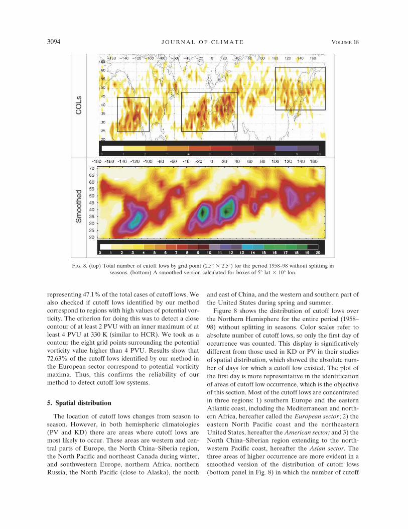
Figure 8 shows the distribution of cutoff lows overthe Northern Hemisphere for the entire period (1958–98) without splitting in seasons. Color scales refer toabsolute number of cutoff lows, so only the first day ofoccurrence was counted. This display is significativelydifferent from those used in KD or PV in their studiesof spatial distribution, which showed the absolute num-ber of days for which a cutoff low existed. The plot ofthe first day is more representative in the identificationof areas of cutoff low occurrence, which is the objectiveof this section. Most of the cutoff lows are concentratedin three regions: 1) southern Europe and the easternAtlantic coast, including the Mediterranean and north-ern Africa, hereafter called the European sector ; 2) theeastern North Pacific coast and the northeasternUnited States, hereafter the American sector; and 3) theNorth China–Siberian region extending to the north-western Pacific coast, hereafter the Asian sector. Thethree areas of higher occurrence are more evident in asmoothed version of the distribution of cutoff lows(bottom panel in Fig. 8) in which the number of cutoff

FIG. 8. (top) Total number of cutoff lows by grid point (2.5° � 2.5°) for the period 1958–98 without splitting inseasons. (bottom) A smoothed version calculated for boxes of 5° lat � 10° lon.


Fig 8 live 4/C

lows was recalculated for boxes 5° latitude � 10° lon-gitude. The three sectors can be more easily identifiedby latitude–longitude boxes, so the European sectorextends from 25° to 47.5°N, 50°W to 40°E; the Ameri-can sector from 25° to 45°N, 100° to 150°W; and theAsian sector from 37.5° to 62.5°N, 100°E to 180°. Ingeneral, these results are concordant with previous par-tial climatologies, although in KD and PV the area ofmost frequent occurrence extended to northern Europeand northeast Canada.

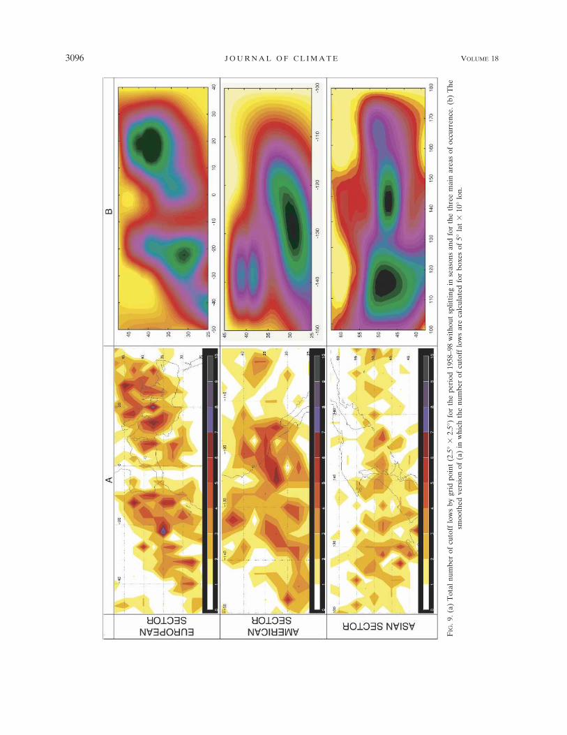
Figure 9 shows a more detailed picture of the geo-graphical distribution of the absolute number of cutofflows for the three main sectors of occurrence. Figureson the left display absolute number of cutoff lows com-puted for 2.5° � 2.5° boxes, and figures on the right aresmoothed versions in which the number of cutoff lowswere recalculated for boxes of 5° latitude � 10° longi-tude. Inside the European sector, there are two areasthat exhibit higher frequencies of cutoff low formation,the eastern Atlantic and the southern parts of the Eu-ropean continent–Mediterranean region. Both pre-ferred areas were already identified in partial clima-tologies of cutoff lows (KD) and in an analysis of geo-graphical distribution of “cold pools” over Europe(Llasat and Puigcerver 1990). However, the easternarea (from the Italian Peninsula to the Balkan Penin-sula) is more clearly defined in our analysis. However,PV did not analyze cutoff low distribution over Europewith this detail, and the regional climatology based onmaxima of potential vorticity (HCR) identified only amaximum close to the Iberian Peninsula. The two areasof higher occurrence in the American sector, at twodifferent latitudes, can be caused by the seasonal cyclesince the main production mechanism responsible forcutoff low formation (meridional displacement of jetstreams) shows a seasonal cycle. In the Asian sector themost frequent occurrence area has a “band” shape be-tween 42.5° and 55°N with two local maxima placed at115° and 140°E.

Studies using long reanalysis data can be affected byinhomogeneities in the observational data, in particularthe introduction of the satellite data in 1979, whichcould result in jumps in climatological quantities withthe introduction of new observing systems. To check ifthe inhomogeneities can affect the climatological quan-tities of cutoff lows, the period of analysis was dividedinto two periods (1958–78 and 1979–98) and the distri-bution of cutoff lows over the Northern Hemisphere forboth periods were calculated (figure not shown). Thereare no clear differences from one period to the otherwith the similar three areas of higher cutoff low occur-rence and with maxima and minima placed on similarpositions.

6. Temporal distribution

Previous climatologies showed that cutoff low sys-tems in the Northern Hemisphere are much more com-mon in summer months, particularly in June and July.Price and Vaughan reported that 30% of cutoff lowsduring 1 October 1982–30 September 1983 occurred inJune and July and KD found that 37% of the cutofflows during the period 1990–94 formed in summer. Theseason with the least number of cutoff lows was clearlywinter (15% in KD for the whole season and 9% in PVfor December and January). The seasonal distributionof cutoff lows showed very similar patterns when it wasdivided into the three types of cutoff lows by PV andfor cutoff lows below 40°N and between 40° and 70°Nin KD.

Figure 10 shows the seasonal distribution of cutofflows for the analyzed period 1958–98 and for each mainsector of occurrence. We can see that the three sectorsshow the same type of seasonal distribution. Cutofflows are much more common in the summer for thethree regions, with 44.6% occurring during this seasonfor the European sector, 49.5% for the American sec-tor, and 58.4% for the Asian sector. During winter, farfewer cutoff lows formed in the three regions, only10.6%, 3.5%, and 5.6% for the European, American,and Asian sectors, respectively. A similar seasonal be-havior found in previous partial climatologies (PV andKD) was attributed to the existence of weaker jetstreams during summer, which allows greater meridi-onal flow and more likelihood in the probability of cut-off low formation. To know if the inhomogeneities inthe reanalysis data can affect the seasonal distributionof cutoff lows we studied the seasonal distribution intwo periods (1958–78 and 1979–98), not finding signifi-cant differences.

To examine geographical differences in the seasonaldistribution, we analyzed the number of cutoff lows foreach season and main sector of occurrence (Fig. 11).Colored areas include at least 95% of the total numberof cutoff lows for each sector and season. Numbers overcolored areas denote places where more than one cut-off low is present in that period. There are substantialseasonal changes in the region of occurrence, so in theEuropean sector most cutoff lows occurred in northernAfrica and southern Europe during winter and extendtoward higher latitudes during the rest of the year. Thebipolar structure shown in section 5, consisting in amaximum over the Atlantic coast and another over theAdriatic Sea, appears in spring, summer, and fall, beingmore expanded during summer. Furthermore, the At-lantic pole is displaced to lower latitudes during fall. Inthe American sector, the area of occurrence is limited


FIG

.9.(

a)T

otal

num

ber

ofcu

toff

low

sby

grid

poin

t(2

.5°

�2.

5°)

for

the

peri

od19

58–9

8w

itho

utsp

litti

ngin

seas

ons

and

for

the

thre

em

ain

area

sof

occu

rren

ce.(

b)T

hesm

ooth

edve

rsio

nof

(a)

inw

hich

the

num

ber

ofcu

toff

low

sar

eca

lcul

ated

for

boxe

sof

5°la

t�

10°

lon.


Fig 9 live 4/C

to the Pacific coast during winter and it is expanded anddisplaced westward and to higher latitudes duringspring and summer. For this season the area of occur-rence is clearly located over the Pacific Ocean since thepercentage of cutoff lows occurring over land are muchmore reduced than during spring. In fall this displace-ment is reversed, most of the cutoff lows being found atlatitudes lower than 35°N and close to the Americancoast. A similar pattern happens in the Asian sector, sothe reduced area over the Japanese coast in winter ex-pands during spring and summer, reaching in this lastseason a higher extension over the continent than overthe ocean.

7. Duration and tracks

A cutoff low system would last about a couple of daysbefore being destroyed by diabatic heating (Hoskins etal. 1985; PV) if there were no injection of new air intothe cutoff low with high potential vorticity. Most cutofflow systems have a short lifetime. In their study, KDfound that the majority of cutoff lows lasted 2–3 daysand very few lasted more than 10 days. In their study,PV found a duration range from 1 to 17 days, althoughmost cutoff lows were short lived (74% of cutoff lowslasted 3 days or less with 41% of them lasting only 1day).

Figure 12 shows the number of cutoff lows lasting 2or more days (excluding 1-day events) as a function ofthe duration. We can notice that most cutoff lows lastedonly 2 days. So, 76.0% for the European sector, 74.3%for the American sector, and 80.3% for the Asian sec-tor lasted only 2 days. Results also show that the num-ber of events lasting 5 or more days is really small

(2.3%, 3.5%, and 1.1% for the European, American,and Asian sectors, respectively). These results confirmKD and PV studies in the sense of the higher frequencyof short-life cutoff lows. However, our procedure ofidentification assigns a shorter life to cutoff lows thanthose used by KD and PV. This could be attributed toour way of tracking since it require contiguous cutofflow points in consecutive days to consider them as thesame cutoff low. To validate this condition, we esti-mated, for the European sector, the percentage of caseswhen nonadjacent cutoff low points in consecutive dayscould belong to the same cutoff low. The left-hand sideof Fig. 13 shows an example of two nonadjacent butclose cutoff low points in consecutive days, with a rela-tively high probability of being the same system. Butonly 16 cutoff lows of a total of 601 (about 2.6%) fulfillthis condition. On the right-hand side of Fig. 13 anotherexample is displayed, but in this case the distance be-tween cutoff low points in consecutive days is higher, sothe probability of being the same system is very re-duced. There are 18 similar cases from a total of 601.Taking into account that some of these cases are notreally the same cutoff low, these percentages are evenlower. So, the differences attributable to the trackingmethod are neglegible. On the other hand, the auto-mated method is more restrictive that subjective meth-ods since we do not allow a time discontinuity in thefullfillment of our conditions. This is not always thecase when a subjective method is applied. In the sub-jective analysis, the identification of a system as a cutofflow, even if some of the conditions defining such asystems are not fulfilled, is relatively frequent. There-fore some discontinuities are inevitably included and alonger life cycle may be found. This is the reason for thesmall discrepancies detected in the comparison.

It has also been suggested that southern cutoff lowslasted less than northern ones, so KD found that theirsubtropical cutoff lows lasted between 2 and 4 days,whereas their polar cutoff lows lasted longer (most ofthem more than 5 days). They justified this result as aconsequence of the injection of fresh polar air that pro-duces a reintensification process in the polar type andnot in the subtropical one. Figure 14 shows the contourplot of duration of our step 3 cutoff lows versus latitudeand longitude. The surface was fit to the XYZ coordi-nate data using the bicubic spline smoothing procedure.White dots represent grid points where cutoff lows oc-curred and the underlined numbers on the figure de-note position and duration of longer cutoff lows. Inboth European and American sectors longer cutofflows also occurred in regions where cutoff lows oc-curred more frequently, which indicates no clear rela-

FIG. 10. Seasonal distribution of the number of cutoff lows forthe three main sectors of occurrence.


FIG

.11.

Num

ber

ofcu

toff

low

sfo

rea

chse

ason

and

mai

nse

ctor

ofoc

curr

ence

.Col

ored

area

sin

clud

eat

leas

tth

e95

%of

the

tota

lnu

mbe

rof

cuto

fflo

ws

for

each

sect

oran

dse

ason

.Num

bers

over

colo

red

area

sde

note

plac

esw

here

mor

eth

anon

ecu

toff

low

was

pres

ent

inth

atpe

riod

.


Fig 11 live 4/C

tionship with latitude. However the area of longer du-ration in the Asian sector (latitude higher than 60°) isclearly different from the area of higher occurrence(latitude band between 45° and 55°). This confirmsKD’s preliminary result that the length of cutoff lowsdepends on latitude only for polar cutoff lows (thoseplaced at latitudes higher than 50°, an area not analyzedin the European and American sectors).

Concerning their mobility, it has been traditionallythought that cutoff lows are quasistationary. This ideacomes from the work by Bell and Bosart (1989), who

found that cutoff low source and dissipation areas in theMediterranean were very close. However, in theiranalysis PV found that almost half of the systemsmoved considerably. This result was confirmed by KD,who linked duration and movement, concluding thatapproximately 50% of the cutoff lows that lasted morethan 3 days moved considerable distances (�600 km).According to these authors, cutoff low motion was, as arule, rather irregular with a trend to move northward,or northeastward, as they began to decay. A more de-tailed analysis appears in the study by Hernández(1999). By analyzing 271 cutoff lows over southeasternEurope, she found two kinds of behavior: those systemsthat were quasi stationary and those moving in a cy-clonic sense with a mean gyre of 20° in 12 h and amaximum movement of 8.75° in longitude and 6.25° inlatitude in 12 h. However, the author recognized thatthe representativeness of this result was weak due tothe high variance in the movement of cutoff lows.

We have analyzed (Fig. 15) the daily displacement ofthe cutoff lows considering that the system is stationary(ST in the figure) if the grid point representative of thecutoff low is the same for the following day. In anyother case we identified the movement by means of thepositions of representative grid points (RGP), as N or Sif the RGP maintains the same longitude, E or W if itmaintains the same latitude, and NE, SE, SW, or NWfor movement between main cardinal points. We havenot considered the length of the displacement in this

FIG. 13. Example of two situations where nonadjacent cutoff low points in consecutive days could belong to thesame system. Case A is an example of close points, when the probability of being the same cutoff low is relativelyhigh. In cases like B the distance between points is higher and this probability is very reduced. Cutoff low pointsdetected as different systems by our method are displayed with different colors (the cutoff low that appears firstis in red). Numbers indicate the number of day in the lifetime of the cutoff lows. Red numbers in brackets besidethe blue ones show this number supposing that both cutoff lows are the same. For example, in case A our methoddetected two cutoff lows during 2 days. For the one in red, day 1 is 14 and day 2 is 15 Mar 1994, whereas for theblue one day 1 is 15 and day 2 is 16 Mar 1994. The day 2 point in red is very close to day 1 point in blue, so thefirst day point of the second cutoff low (1 in blue) could actually be a part of the first cutoff low in its second day(2 in red between brackets).

FIG. 12. Number of cutoff low events as a function of theduration for the three main sectors of occurrence.


Fig 13 live 4/C

analysis. What the analysis accounts for is the differentmovement from the first day of occurrence to the sec-ond, the second to the third, the third to the fourth, andthe fourth to any subsequent day. Results from this lasttransition—fourth to any other day—should be cau-tiously considered because of the reduced number ofcases. Our results confirm that the number of stationarycutoff lows is lower than initially expected. Cutoff lowstend to move any time during their life cycle. So thepercentage of stationary cutoff lows from the first dayof occurrence to the second is 14.8%, 21.9%, and 13%for the European, American, and Asian sectors, respec-tively. This percentage distribution is very similar forthe second to the third day and for the third to thefourth day in the American sector where cutoff lowstend to be more stationary. The result reached by PV,that cutoff lows often moved in latitude or longitudebut fewer systems moved in both latitude and longi-tude, was not found in our analysis as a general rule.The single transition where this happened was from thesecond to the third day. In this case the ratio betweensystems moving only in latitude or longitude versus sys-tems moving both in latitude and longitude was 1.66,1.23, and 1.71 for the European, American, and Asiansectors, respectively. As in PV and KD, we found con-siderable difficulty defining favored tracks for cutofflow systems, as their movement appeared to be ratherirregular. In general, most of the systems move north-ward, so the ratio between movements northward (N,NW, and NE) and southward (S, SW, and SE) is 1.78,1.85, and 2.48 for the first to the second day in theEuropean, American, and Asian sectors, respectively,and similar results were reached for the second to thethird day. In the transition from the third to the fourthday this preference of northward movement is notpresent in the American sector and it is not represen-tative in any sector for the remaining transitions. Thisresult contrasts with studies by PV or KD, where thenorthward displacement was more evident as the cutofflow started to decay. The possibly eastward displace-ment suggested by KD was not confirmed. In our study,European cutoff lows moved eastward in the transitionfrom the first to the second day and westward in therest of transitions. So, the ratio between westwardmovements (W, NW, and SW) and eastward move-ments (E, NE, and SE) is 0.59, 1.30, 1.73, and 2.5 for thefour studied transitions. In the American sector, cutofflows tend to move westward in any of the transitions, sothe relationship westward–eastward is 1.20, 1.73, 3.0,and 3.5. In the Asian sector the westward movement isonly dominant in the transitions from the second to thethird day and from the third to the fourth day.

FIG. 14. Contour plot of duration of cutoff lows vs latitude andlongitude (the surface was fit to the XYZ coordinate data usingthe bicubic spline smoothing procedure). White dots representgrid points where cutoff lows occurred and the number on thefigures denote position and duration of longer cutoff lows.


Fig 14 live 4/C

8. Conclusions

This study provides the first multidecadal (41 yr) cli-matology of cutoff low systems in the Northern Hemi-sphere. Cutoff lows were identified using data from theNCEP–NCAR reanalysis and an objective methodbased on imposing the three main physical characteris-

tics of the conceptual model of cutoff low. In generalterms, the agreement between our objective methodand the subjective procedures used in previous studiesis good in extratropical areas, the method underesti-mates the number of cutoff lows when compared withprevious studies in near-polar or polar regions and itoverestimates cutoff lows for subtropical or even tropi-

FIG. 15. Daily movement of the cutoff lows calculated as displacement of the representative grid point: STindicates the number of stationary systems; N, NE, E, SE, S, SW, W) and NW indicates the number of cutoff lowsmoving toward that cardinal point. The analysis was done for four different transitions: from the first day ofoccurrence to the second, the second to the third, the third to the fourth, and the fourth to any other day.


cal areas. Independent of these small disagreements,the long-term cutoff low database built is an appropri-ate tool to study the interannual variability of cutofflow occurrence and the links between cutoff lows andjet stream systems, blocking, or major modes of climatevariability. From our study, some new interesting prop-erties of cutoff low systems have been revealed andothers previously well known have been validated.

There are three preferred areas of cutoff low occur-rence: southern Europe and the eastern Atlantic coast,the eastern North Pacific, and the North China–Siber-ian region extending to the northwestern Pacificcoast—the European area being the most favored re-gion. This result shows that cutoff lows occur preferen-tially near the major troughs of the large-scale circum-polar flow. As suggested in PV and KD, the seasonalvariations in latitudinal temperature gradients and tem-perature contrasts between continental and oceanic re-gions seems to be ultimately responsible for the sea-sonal cycle in the number and position of cutoff lowsthrough seasonal variations in the jet system. This hy-pothesis can now be checked by using this long-termcutoff low database and will be one of the major objec-tives of a following paper. Cutoff lows form much moreoften in summer than in winter and at higher latitudes.About 50% of all the identified cutoff lows occurredduring summer and 30% during spring, and this result iscommon for the three main areas of occurrence. Amore exhaustive analysis of the areas of occurrenceshowed a bimodal distribution in Europe in all the sea-sons with the exception of winter, a summer displace-ment to the ocean in the American region, and a sum-mer extension to the continent in the Asian region.These results are possibly related to the strength andposition of the jet system during summer. Weaker jetscoupled with the warmer continental areas are respon-sible for increasing the meridional flow in these regionsof the Northern Hemisphere. Most cutoff lows lasted2–3 days and very few lasted more than 5 days. Al-though with limitations, cutoff lows lasted longer whenthey occurred at higher latitudes. We also examined themobility of cutoff lows. In general, most of them aremobile any day of their life cycle, with less than 20%being stationary. In most cases a northward and west-ward motion was evident, especially in the transitionsfrom the second to the third day of occurrence andfrom the third to the fourth day.

In general, this first multidecadal and objective cli-matology of cutoff lows is in good agreement with pre-vious 1–5 yr and subjective analyses, and confirmsmany of the known characteristics of cutoff lows, espe-cially the main areas of occurrence and the seasonaldistribution of occurrence. Other characteristics, such

as the movement and duration of the systems, wereonly partially confirmed, finding a trend to move west-ward and a duration shorter than estimated in previousstudies. Furthermore, the long period permitted us todefine the seasonal variability for the areas of occur-rence.

Acknowledgments. This work was supported by theSpanish Ministry and Science and Technology (MCYT)under Grant REN2002-04558-C04-02 and by the Gali-cian Programme of Research and Development underGrant PGIDIT03PXIC38301PN. The authors thankthree anonymous reviewers for their helpful commentsand suggestions.

REFERENCES

Bamber, D. J., P. G. W. Healey, B. M. R. Jones, S. A. Penkett,A. F. Tuck, and G. Vaughan, 1984: Vertical profiles of tro-pospheric gases: Chemical consequences of stratospheric in-trusions. Atmos. Environ., 18, 1759–1766.

Bell, G. D., and L. F. Bosart, 1989: A 15-year climatology ofNorthern Hemisphere 500 mb closed cyclone and anticyclonecenters. Mon. Wea. Rev., 117, 2142–2163.

Cuevas, E., and J. Rodríguez, 2002: Statistics of cutoff lows overthe North Atlantic (in Spanish). Proc. Third Asamblea His-pano-Portuguesa de Geodesia y Geofísica, Valencia, Spain,Comision Española de Geodesia y Geofisica, 1–3.

——, D. V. Henriques, and J. M. Sancho, 2000: Stratosphere–troposphere exchange events over North Atlantic subtropicalregion. Proc. Second Asamblea Hispano-Portuguesa de Geo-desia y Geofísica, Lagos, Portugal, Comision Española deGeodesia y Geofisica, 451–452.

García-Herrera, R., D. G. Puyol, E. H. Martín, L. G. Presa, andP. R. Rodríguez, 2001: Influence of the North Atlantic Oscil-lation on the Canary Islands precipitation. J. Climate, 14,3889–3903.

Gimeno, L., E. Hernández, A. Rúa, and R. García, 1998: Surfaceozone in Spain. Chemosphere, 38, 3061–3074.

Hernández, A., 1999: Un Estudio Estadístico sobre DepresionesAisladas en Niveles Altos (DANAs) en el Sudoeste de Eu-ropa basado en Mapas Isentrópicos de Vorticidad Potencial.IV Simposio Nacional de Predicción, Instituto Nacional deMeteorología, Serie Monogr., No. SM 351, Ministerio de Me-dio Ambiente, 235 pp.

Hill, E. F., and K. A. Browning, 1987: Case study of a persistentmesoscale cold pool. Meteor. Mag., 116, 297–309.

Holton, J., P. Haynes, M. McIntyre, A. Douglass, R. Rood, and L.Pfister, 1995: Stratosphere–troposphere exchange. Rev. Geo-phys., 33, 403–439.

Hoskins, B. J., M. E. McIntyre, and A. W. Robertson, 1985: Onthe use and significance of isentropic potential vorticity maps.Quart. J. Roy. Meteor. Soc., 111, 877–946; Corrigendum, 113,402–404.

Kalnay, E., and Coauthors, 1996: The NCEP/NCAR 40-Year Re-analysis Project. Bull. Amer. Meteor. Soc., 77, 437–471.

Kentarchos, A. S., and T. D. Davies, 1998: A climatology of cutofflows at 200 hPa in the Northern Hemisphere, 1990–1994. Int.J. Climatol., 18, 379–390.

——, G. J. Roelofs, J. Lelieveld, and E. Cuevas, 2000: On the


origin of elevated surface ozone concentrations at Izana Ob-servatory during the last days of March 1996: A model study.Geophys. Res. Lett., 27, 3699–3702.

Keyser, D., and M. A. Shapiro, 1986: A review of the structureand dynamics of upper level frontal zones. Mon. Wea. Rev.,114, 452–499.

Llasat, M. C., and M. Puigcerver, 1990: Cold pools over Europe.Meteor. Atmos. Phys., 42, 171–177.

Matsumoto, S. K., K. Ninomiya, R. Hasegawa, and Y. Miki, 1982:The structure and role of a subsynoptic cold vortex on theheavy precipitation. J. Meteor. Soc. Japan, 60, 339–353.

Novak, M. J., L. F. Bosart, D. Keyser, T. A. Wasula, and K. D.LaPenta, 2002: Climatology of warm season 500 hPa cutoffcyclones and a case study diagnosis of 14–17 July 2000. Pre-prints, 19th Conf. on Weather Analysis and Forecasting, SanAntonio, TX, Amer. Meteor. Soc., 68–71.

Oltmans, S., and Coauthors, 1996: Summer and spring ozone pro-files over the North Atlantic from ozonesonde measure-ments. J. Geophys. Res., 101, 29 179–29 200.

Palmén, E., and C. W. Newton, 1969: Atmospheric CirculationSystems: Their Structure and Physical Interpretation. Aca-demic Press, 603 pp.

Parker, S. S., J. T. Hawes, S. J. Colucci, and B. P. Hayden, 1989:Climatology of 500 mb cyclones and anticyclones 1950–85.Mon. Wea. Rev., 117, 558–570.

Price, J. D., and G. Vaughan, 1992: Statistical studies of cutoff-lowsystems. Ann. Geophys., 10, 96–102.

——, and ——, 1993: The potential for stratosphere–troposphereexchange in cut-off low systems. Quart. J. Roy. Meteor. Soc.,119, 343–365.

Winkler, R., and Coauthors, 2000: Manual of synoptic satellitemeteorology: Conceptual models, version 5.0. [Availablefrom Central Institute for Meteorology and Geodynamics,Hohe Warte 38, 1190 Vienna, Austria.]

Wirth, V., 1995: Diabatic heating in an axisymmetric cutoff cy-clone and related stratosphere–troposphere exchange. Quart.J. Roy. Meteor. Soc., 121, 127–147.


climatological features of cutoff low systems in the...

Documents