climatic and ecological determinants of leaf lifespan in ... · pdf filepolar forests once...

Climatic and ecological determinants of leaflifespan in polar forests of the high CO2 Cretaceous‘greenhouse’ world

S . J . B R E N T N A L L *, D . J . B E E R L I N G *, C . P. O S B O R N E *, M . H A R L A N D w , J . E . F R A N C I S w ,

P. J . VA L D E S z and V. E . W I T T I G §

*Department of Animal and Plant Sciences, University of Sheffield, Sheffield S10 2TN, UK, wSchool of Earth and Environment,

University of Leeds, Leeds LS2 9JT, UK, zSchool of Geographical Sciences, University of Bristol, Bristol BS8 1SS, UK, §Department

of Plant Biology, University of Illinois at Urbana-Champaign, IL 61801-3838, USA

Abstract

Polar forests once extended across the high-latitude landmasses during ice-free ‘green-

house’ intervals in Earth history. In the Cretaceous ‘greenhouse’ world, Arctic conifer

forests were considered predominantly deciduous, while those on Antarctica contained a

significantly greater proportion of evergreens. To investigate the causes of this distinctive

biogeographical pattern, we developed a coupled model of conifer growth, soil biogeo-

chemistry and forest dynamics. Our approach emphasized general relationships between

leaf lifespan (LL) and function, and incorporated the feedback of LL on soil nutrient

status. The model was forced with a mid-Cretaceous ‘greenhouse’ climate simulated by

the Hadley Centre GCM. Simulated polar forests contained mixtures of dominant LLs,

which reproduced observed biogeographical patterns of deciduous, mixed and evergreen

biomes. It emerged that disturbance by fire was a critical factor. Frequent fires in

simulated Arctic ecosystems promoted the dominance of trees with short LLs that were

characterized by the rapid growth and colonization rates typical of today’s boreal pioneer

species. In Antarctica, however, infrequent fires allowed trees with longer LLs to

dominate because they attained greater height, despite slower growth rates. A direct

test of the approach was successfully achieved by comparing modelled LLs with

quantitative estimates using Cretaceous fossil woods from Svalbard in the European

Arctic and Alexander Island, Antarctica. Observations and the model both revealed

mixed Arctic and evergreen Antarctic communities with peak dominance of trees with

the same LLs. Our study represents a significant departure from the long-held belief that

leaf habit was an adaptation to warm, dark winter climates, and highlights a previously

unrecognized role for disturbance (in whatever guise) in polar forest ecology.

Keywords: biogeochemistry, disturbance, fossils, leaf lifespan, modelling, polar forests

Received 18 February 2005; and accepted 1 August 2005

Introduction

Fossil evidence indicating that forests once extended to

latitudes of 851N and S provides a tangible reminder of

a unique, but now extinct, biome existing for at least the

last 350 million years of Earth history (Spicer & Chap-

man, 1990). In stark contrast with today’s high-latitude

forests, this biome flourished in a warm ‘greenhouse’

climate with high atmospheric CO2 levels (Crowley &

Berner, 2001), mild, possibly frost-free winter tempera-

tures (Tarduno et al., 1998; Tripati et al., 2001; Dutton

et al., 2002) and, at a latitude of 851, experienced 5

months of darkness during the polar winter and an

equal period of continuous sunlight during the sum-

mer. Since the late 1940s, the predominant world view

of polar forests has been that their deciduous character

represented an adaptation to winter darkness, allowing

the trees to avoid the high respiratory losses associated

with maintaining a canopy of leaves during the warm

winter (Chaney, 1947; Axelrod, 1966; Hickey, 1984;

Wolfe, 1985). However, this carbon balance view wasCorrespondence: David Beerling,

e-mail: [email protected]

Global Change Biology (2005) 11, 2177–2195, doi: 10.1111/j.1365-2486.2005.01068.x

r 2005 Blackwell Publishing Ltd 2177

not universally accepted, even at the time it was first

proposed (Mason, 1947; Creber & Chaloner, 1985; Read

& Francis, 1992), and results from recent experiments

and numerical modelling studies (Beerling & Osborne,

2002; Osborne & Beerling, 2003; Royer et al., 2003, 2005)

have failed to provide supporting evidence. Indeed,

under experimental conditions, the quantity of carbon

lost annually by deciduous trees through leaf shedding

exceeded that lost by evergreen trees through winter

respiration and more limited leaf loss (Royer et al., 2003,

2005). Even at the scale of whole forest ecosystems, the

deciduous leaf habit was approximately twice as ex-

pensive in terms of winter carbon loss as its evergreen

counterpart.

Our understanding of the significance of leaf habit for

polar forest ecology therefore requires rethinking (Os-

borne et al., 2004). We suggest attention might usefully

shift from the simple evergreen vs. deciduous dichot-

omy towards one considering leaf lifespan (LL, average

leaf retention time) along a continuous spectrum run-

ning from a quick to slow return on investments of

nutrient and dry mass (Kikuzawa, 1991; Reich et al.,

1997; Givnish, 2002; Grubb, 2002; Wright et al., 2004).

Global surveys reveal that key leaf traits dictating

resource investment and return vary with LL in a

manner that alters vegetation function (e.g. evapotran-

spiration, net primary productivity (NPP)), structure,

and nutrient cycling (e.g. albedo, tree height) (Reich

et al., 1997, 1999; Wright et al., 2004). These emerging

views of leaf investment strategies are particularly

timely in the context of polar forests because new

techniques in palaeobotany now allow estimation of

LL for extinct species by analysing cellular patterns in

the growth rings of fossil wood (Falcon-Lang, 2000a, b).

LL, therefore, provides a promising means of realisti-

cally uniting past and present forest ecology, and in-

vestigating the underlying reasons for the composition

of long-extinct high-latitude forests, whose dynamics

cannot be inferred directly from fossil remains.

Here, we present a numerical modelling investigation

developing this new line of ecological enquiry for the

conifer-dominated polar forests of the Cretaceous. We

analyse the effect of LL on the functioning of polar

forests, with the aim of determining its significance for

forest composition, a product evaluated against the

fossil record. Critically, we interrogate model simula-

tions to uncover the key mechanisms responsible for

distinctive patterns of polar forest biogeography now

beginning to emerge from the fossil record (Spicer &

Parrish, 1986; Falcon-Lang & Cantrill, 2000, 2001a, b).

These indicate that, rather than being of a uniformly

deciduous character, high-latitude forests of the Cretac-

eous were deciduous in the Arctic region, but predo-

minantly evergreen in Antarctica.

Our approach utilizes the University of Sheffield

Conifer Model (USCM), a process-based forest growth

model that scales-up from generalized relationships

between LL, leaf traits and climate (Osborne & Beerling,

2002a). The USCM has been extended and modified by

coupling it with a soil biogeochemistry module (Parton

et al., 1993) to incorporate self-consistent nutrient lim-

itations by simulating belowground carbon and nitro-

gen cycling. Simulated structural and functional

characteristics of trees drive a forest dynamics scheme

in which height is determined from hydraulic con-

straints, wood production and time since last distur-

bance (Whitehead et al., 1984; Margolis et al., 1995;

Osborne & Beerling, 2002b), and Lotka–Volterra equa-

tions for representing interspecific competition (Silver-

town & Lovett-Doust, 1993; Cox, 2001).

We focus on the mid-Cretaceous (Aptian, 124–112 Ma)

because it represents a time of global warmth (Spicer &

Corfield, 1992) and the heyday of polar forests (Spicer &

Parrish, 1986). We developed both qualitative and

quantitative palaeodatasets to evaluate simulations of

polar forest distribution and composition against ob-

servations. The qualitative dataset was compiled by

analysing information from published sources describ-

ing the presumed leaf habit (evergreen vs. deciduous)

of fossil plant assemblages and has the more extensive

geographical coverage. While it only gives an indication

of the predominant leaf habit for forests at a particular

locality, it highlights regional-scale biome distributions

and serves as a valuable guide for evaluating model

performance. The quantitative dataset provides esti-

mates of LL for comparison with USCM predictions

and derives from analysis of Cretaceous fossil woods

from Svalbard in the high northern latitudes (this

paper) and Alexander Island, Antarctica (Falcon-Lang

& Cantrill, 2000, 2001a, b; Falcon-Lang, 2000a, b).

Materials and methods

Coupled USCM description

The forest growth module of the coupled USCM, de-

scribed and validated in detail elsewhere (Osborne &

Beerling, 2002a), considers four biogeochemical and

biophysical aspects of forest function in relation to LL:

(i) carbon exchange between vegetation and the atmo-

sphere; (ii) fluxes of water through the soil–plant–atmo-

sphere continuum; (iii) limitation of tree growth by

nitrogen; and (iv) land surface-atmosphere energy ex-

change. In the model, LL directly influences the nitro-

gen content of tissues and leaf mass: area ratios (Reich

et al., 1998; 1999), which then determine leaf capacities

for photosynthesis, respiration and stomatal conduc-

tance. Photosynthetic carbon uptake is described by the

2178 S . J . B R E N T N A L L et al.

r 2005 Blackwell Publishing Ltd, Global Change Biology, 11, 2177–2195

Farquhar et al. (1980) biochemical model and scaled to

the canopy using a ‘sun-shade’ approach (DePury &

Farquhar, 1997). This canopy scheme accounts for dis-

tributions of nitrogen and photosynthetic enzymes

within the canopy, and sunlit and shaded fractions of

leaves. Plant respiration is dependent upon tempera-

ture and tissue nitrogen contents (Ryan et al., 1996).

Evapotranspiration follows the Penman–Monteith

method (Penman, 1948; Monteith, 1965), accounting

for stomatal responses to soil water, atmospheric hu-

midity and CO2 (Leuning, 1995), the dependence of

aerodynamic roughness on canopy leaf area (Shaw &

Pereira, 1982), and the limitation of soil evaporation by

surface moisture content (Chanzy & Bruckler, 1993).

Nitrogen uptake depends on the mass of roots, tem-

perature and soil nitrogen content (Woodward et al.,

1995). A further limitation is imposed by the soil carbon

content, which influences mycorrhizal associations of

trees and their ability to extract organic nitrogen (Wood-

ward & Smith, 1994). Energy exchange between vegeta-

tion, soil and the atmosphere accounts for short-wave,

long-wave (upward and downward), latent and sensi-

ble heat fluxes. The absorption of solar energy in both

the visible and near-infrared wavebands is considered

for the leaf canopy and soil (Weiss & Norman, 1985;

DePury & Farquhar, 1997). Forest energy budget, eva-

potranspiration and photosynthesis are interdependent,

and solved numerically. The leaf area index (LAI), a key

determinant of energy, water and carbon fluxes in

the model, is calculated after accounting for the limita-

tions on growth imposed by water, nitrogen and light

(Osborne & Beerling, 2002a).

The soil module newly incorporated for this paper is

based upon the Century model of carbon and nitrogen

dynamics (Parton et al., 1993) (Fig. 1). Eight soil carbon

and nitrogen pools are modelled, each distinguished by

their different maximum decomposition rates: two sur-

face litter pools, representing the more recalcitrant (e.g.

lignin, cellulose) and more labile (e.g. sugars) compo-

nents, respectively, two similar pools for subsurface

(especially root) litter; surface and soil microbial (active)

pools; and pools of slow and passive soil organic matter

(Fig. 1). Decomposition rates, and fluxes of carbon

between the pools, are calculated as functions of soil

moisture and temperature. Nitrogen fluxes and the C : N

ratio of each reservoir are controlled by the size of a

further pool, mineral nitrogen, which is in turn affected

by the implied net mineralization or immobilization of

the other pools. Each nitrogen flux is equal to the

product of the corresponding carbon flux and the N : C

ratio of the pool receiving the flow. Soil carbon and

nitrogen dynamics are described by nonlinear differen-

tial equations with parameters depending on soil tex-

ture, temperature, precipitation, humidity, soil moisture,

water flow, potential evaporation, litter quantity and

quality. The equations are solved on a monthly time step.

Vegetation module

Soil nutrient cycling module

Surface and root litter C and N pools

Microbial C and N pools

Slow C and N pools

Passive C and N pools

Leaflifespan

CO2

Climate

Hours to years

Months to years

SoilN and H2O

Leaf-scaleprocesses

Tree-scaleprocesses

Ecosystem-scaleprocesses

Surface and root litter,C : N ratios

Fig. 1 Schematic diagram of key forest processes from the leaf to the regional scale simulated in the above- and below-ground modules

of the University of Sheffield Conifer Model.

S I M U L AT I N G C R E T A C E O U S P O L A R F O R E S T S 2179


The model requires inputs of monthly temperature,

relative humidity and precipitation, which for the Cre-

taceous simulations were derived from the Hadley

Centre general circulation model (GCM). Successful

validation of the USCM under the present-day climate

and atmospheric CO2 concentration was achieved on a

site-by-site basis by comparing predictions and obser-

vations of LAI and NPP from conifer forest across a

wide climatic gradient and, at the regional scale, by

comparison with satellite products (see Appendix A).

Forest dynamics scheme

The coupled USCM simulates the properties of a mono-

culture forest of a given LL growing within each grid-

box. We performed parallel simulations for trees with a

range of LLs, to determine the composition of the forest

using a form of Lotka–Volterra dynamics. In this

scheme, the exponential rate of colonization by trees

of each LL is limited by both intra- and interspecific

competition. Competition is proportional to the product

of the two population sizes in question (Silvertown &

Lovett-Doust, 1993). Inclusion of intraspecific competi-

tion means that the growth term can alternatively be

seen as logistic. The version we use also includes a term

representing exogenous mortality because of fire, giving

(Cox, 2001):

Cidvi

dt¼ liPivi 1�

Xn

j¼1

cijvj

8<:

9=;� gvviCi; ð1Þ

where i 5 1, 2, . . . , n is an index for each of the

functional types (FTs) considered. Ci is biomass C per

unit land surface area for the FT with the ith LL, and

vi the fraction of the grid-box covered by trees of this

type. li is a partitioning coefficient representing the

fraction of NPP used for increasing tree numbers, rather

than the size of individual trees (i.e. l is a measure of

the reproductive effort). Pi is the aboveground NPP per

unit vegetated area (g C m�2 yr�1), cij is a competition

coefficient in the range [0, 1] representing the effect on

FT i of type j, and gv is a large-scale disturbance rate.

Disturbance by fire is computed with a fire module,

based on temperature and precipitation, and which has

been validated against satellite wildfire datasets (Beer-

ling & Woodward, 2001; Woodward et al., 2001).

Early successional woody plant species generally

have faster rates of photosynthesis and respiration,

higher stomatal conductance, and more efficient nutri-

ent uptake mechanisms, than their late successional

counterparts (Bazzaz, 1979, 1996; Grime, 2001), all traits

strongly associated with shorter LLs (Reich et al., 1999;

Wright et al., 2004). Consistent with this observation,

trees of relatively short LL, for instance larches, birches,

aspen or white pine, commonly act as pioneer species

after disturbance in today’s boreal or Alpine forests

(Didier, 2001; Schulze et al., 2002; Dole&al et al., 2004;

Jain et al., 2004). Although some of these pioneer species

are deciduous angiosperms, we assume that function-

ally similar gymnosperms fulfilled this role in the Early

to mid-Cretaceous, when angiosperms had not yet

evolved to the point of becoming dominant trees

(Crane, 1987; Hill & Scriven, 1995). To reflect the ten-

dency for trees of shorter LL to be more effective

colonizers, we define the partitioning coefficient l (for

each i) to be a decreasing function of LL, and an

increasing function of LAI, as follows. Denoting LL

(in months) by L, we set l to zero, so that all the

production is channelled towards increasing the size

of individual trees, if the LAI is less than

Lmin ¼0 if L < 4;ðL� 4Þ=24 if 4 � L � 28;1 if 28 < L:

8<: ð2Þ

If the LAI is greater than

Lmax ¼ðLþ 44Þ=12 if L � 68;9 otherwise;

�ð3Þ

then l is set to 1, so that essentially all the production of

mature trees goes towards reproduction. l varies linearly

between these two values of LAI, for a given value of LL.

Thus, the shorter the LL, the lower the LAI at which

some of the production is diverted towards colonization;

and the larger the LAI (for a given LL), the larger the

fraction of production going towards colonization.

We define the competition coefficients as follows

(Cox, 2001):

cij ¼1; i ¼ j;1=½1þ expf20ðhi � hjÞ=ðhi þ hjÞg�; i 6¼ j;

�; ð4Þ

where hi is the height attained by trees of type i in one

fire return interval. This represents competition for

light. If hj � hi, the coefficient is close to 1; tree type j,

being much taller than type i, exerts a large negative

influence on the latter through shading. Conversely, if

hj � hi the coefficient approaches zero.

At equilibrium, dvi/dt 5 0, and (1) becomes a system

of n linear simultaneous equations in the vegetated

fractions vi, provided that these are all nonzero. In

matrix notation, this system is

Cv ¼ a; ð5Þ

where C is the n�n matrix of competition coefficients

cij, v the vector of vegetated fractions, and a is a

vector with elements

ai ¼ 1� gvCi

liPi: ð6Þ

Note that ai is the vegetated fraction that would be

obtained if C were the unit matrix (i.e. represents the



potential vegetated fraction achieved in the absence of

competition from other tree types). It is less than 1

because only a finite time, 1/gv, is available for recolo-

nization between disturbances, the colonization rate,

proportional to lP/C, is also finite, and the colonization

process is effectively logistic (i.e. self-limiting). The

faster the colonization rate, compared with the distur-

bance frequency, the closer the potential vegetated

fraction is to 1. Conversely, if gvCi/liPi41 (i.e. the

disturbance exceeds the colonization rate) we set

ai 5 0; this represents, for example, the case where trees

do not grow vigorously enough to set seed, and sub-

sumes the case where LAI oLmin (i.e. l5 0). Note that

Ci/Pi has units of time, and represents the turnover

time taken for the biomass to be replenished by new

production in the dynamic equilibrium between pro-

duction and decomposition. Therefore, Pi/Ci is a stand-

level growth rate, and liPi/Ci a measure of the rate at

which disturbed land is recolonized by trees of type i, in

the absence of competition.

We solved Eqn (5) at each grid point by inverting C,

after excluding LLs unable to grow (or reproduce) at

that site because of the climate. The final vegetated

fractions are given by

v ¼ C�1a: ð7Þ

This sometimes yields negative vi values, indicating that

type i is outcompeted to extinction; in this case vi is set

to zero.

The (potential) aboveground biomass Cpoti g C m�2� �

accumulating if the trees were allowed to grow to their

full height hmaxi (m), undisturbed by fire or competition,

is calculated as the product of the mass of a single trunk

and the number of trees per unit area (Enquist et al.,

1998). Representing a tree trunk as a cylinder of radius

hmaxi =100, height hmax

i and density 392 kg m�2, of which

40% is carbon (Osborne & Beerling, 2002b), the potential

aboveground biomass is given by

Cpoti ¼ 1251ðhmax

i Þ3=4: ð8Þ

The USCM calculates hmaxi using the hydraulic model of

Whitehead et al. (1984), in which height is inversely

proportional to the square root of an evaporative de-

mand (Koch et al., 2004). Since stomatal conductance

and therefore evaporative demand decrease with in-

creasing LL, trees with longer-lived leaves tend to be

taller, other things being equal (see Osborne & Beerling,

2002b).

Assuming that biomass carbon accumulates annually

according to the NPP until this maximum or equilibrium

value is reached, or until disturbance occurs (whichever

happens first), the final tree height is given by

hi ¼ min hmaxi ;

Piðhmaxi Þ1=4

1251gv

!ð9Þ

and the required biomass Ci is obtained by using

this value for the height in the right-hand side

of Eqn (8). The structure of our FT model is illustrated

in Fig. 2.

To obtain polar biome maps suitable for comparison

with our qualitative palaeodataset, and for validation

against modern data, vegetated fractions vi with differ-

ent LLs were aggregated to give ‘deciduous’ fd (LL o12

months) and ‘evergreen’ fractions fe (LL � 12 months).

The results of this procedure were not sensitive to the

number of different deciduous and evergreen LLs used.

Dominant LLs were defined according to vi. Biome

distribution was optimized through Eqns (2) and (3),

Reproductiveeffort

(�, LAI)

Stand-levelgrowth rate(NPPi/Ci)

Colonizationrate

(�NPP/Ci)

Firefrquency

(1/�)

Potential vegetatedfration of a given

c LL (a)

Actual vegetatedfration of a given

c LL (v)

Competitionwith other LLs

(C,hi)

Fig. 2 Diagrammatic representation of the forest dynamic scheme implemented with the University of Sheffield Conifer Model. Stand-

level growth is partitioned between either reproduction or colonization and over a specific time that depends on disturbance by fire, and

leads to the potential cover of a given pixel. The actual vegetation cover determined by competition with other trees with leaves of

different leaf lifespans.



and fd and fe, to reproduce the extent of northern boreal

forest biomes (evergreen and deciduous needle-leaved

trees) categorized by the International Satellite Land

Surface Climatology Project (ISLSCP) (Meeson et al.,

1995). The k statistic is a measure, albeit imperfect

(Beerling & Woodward, 2001), of how well categorical

dataset reproduces another, and was highly significant

(k5 24.3%, Po0.001).

Mid-Cretaceous global climate simulation

We forced the coupled USCM with a mid-Cretaceous

(Aptian) climate simulation produced by the latest

generation of the Hadley Centre Atmospheric GCM

(HadAM3) (Pope et al., 2000). HadAM3 is based on

the UK Meteorological Office GCM (Hewitt & Mitchell,

1996) and operates with a spatial resolution of 3.751

longitude� 2.51 latitude and 19 vertical levels. Pre-

scribed zonally symmetric sea-surface temperatures

(SSTs) of 30cos(lat) 1C were used; implying an increased

poleward transport of the ocean heat flux compared

with the present day situation. The simulation em-

ployed the reconstructions of mid-Cretaceous coastlines

and the positions of major mountain ranges described

by Smith et al. (1994). Atmospheric CO2 levels were set

at 1300 ppm as the mean of the various proxy estimates

(Crowley & Berner, 2001; Royer et al., 2004). The inte-

gration was run for 14 model years and the Aptian

‘climate’ taken as the average of the last 10 years.

Numerical model experiments

The USCM was run separately for trees with nine

different LLs (4, 6, 9, 12, 18, 24, 48, 72 and 96 months),

using both a modern climatology for the years 1982–

1991, derived from the UEA dataset (New et al., 1999,

2000), and an Aptian climatology as modelled by

HadAM3. Both climatologies were global in extent, at

a resolution of 3.751 in both latitude and longitude.

Polar forest reconstructions

A qualitative dataset of polar and temperate forest

biome distributions in the Early and Late Cretaceous

was compiled from published literature sources (Table

1). Biomes were classified as deciduous, mixed or ever-

green using evidence from macrofossil floras (leaf and

wood), palynological records or the analysis of dis-

persed leaf cuticles. We followed the published inter-

pretations of fossil records in assigning biome types

which used a range of methods to obtain evidence

about leaf habit: wood anatomy (Falcon-Lang,

2000a, b); analysis of leaf traces (Falcon-Lang & Cantrill,

2001a); examination of leaf physiognomy and cuticle

morphology (Chaloner & Creber, 1990); comparison

with nearest living relatives (NLRs) (Chaloner & Creber,

1990); and interpretation of taphonomy (preservational

setting) (Spicer & Parrish, 1986). While none of these

methods is without its difficulties, we have accepted at

face value the authors’ original interpretation, but at-

tempted to draw upon more than one line of evidence

when possible for any particular site.

Wood anatomy provides a proxy record of leaf habit

that is proving useful in palaeoecological reconstruc-

tions (Falcon-Lang & Cantrill, 2000, 2001a, b). It is based

on the general observation that trees with short-lived

leaves produced pronounced annual growth rings,

whereas those with long-lived foliage form less distinct

ring boundaries (Falcon-Lang, 2000a, b). Leaf traces

connect the vascular system of leaves with the xylem

of branch wood in tree species, are extended by sec-

ondary growth every year that the leaf persists, and

remain in wood after leaf abscission. Palaeobotanists

may therefore obtain a very precise measure of LL from

fossil woods by counting the number of annual growth

rings bisected by the xylem strand of leaf traces,

although these are infrequently preserved (Falcon-Lang

& Cantrill, 2001a, b). Physiognomy describes the form

and structure of fossils, and may be used to provide

clues about the habit of leaves, via characters such as

leaf or cuticle thickness and sunken stomata (Chaloner

& Creber, 1990), although these are necessarily spec-

ulative. The NLR method assumes that closely related

fossil and modern plant taxa share common traits such

as LL, but is difficult to apply for the Cretaceous, where

the phylogenetic distance between ancient and modern

species is significant (Chaloner & Creber, 1990). Taph-

onomy is the study of the depositional and fossilization

process, and may provide important inferences about

leaf habit, especially through the interpretation of leaf

mats as characteristic of deciduous species, with leaves

spread randomly throughout a sequence characterizing

evergreens (Spicer & Parrish, 1986).

We obtained new quantitative datasets for LL by

analysing Cretaceous fossil conifer woods using the

approach of Falcon-Lang (2000a, b). The technique fol-

lows from the observation that the markedness of

boundaries between annual growth rings in modern

trees from seasonal climates is correlated with LL

(Falcon-Lang, 2000a, b). To obtain LLs for fossil woods,

we, therefore, used a newly developed modern calibra-

tion dataset for contemporary conifers consisting of 21

modern tree species, with nineteen from the Northern

Hemisphere and two from the Southern Hemisphere

(Harland, 2005). For each genus, the ring markedness

index (RMI) was calculated as RMI 5 PD�PL/100,

where PD is the percentage diminution and PL the

percentage latewood (Falcon-Lang, 2000a, b). The PD



Table 1 Leaf habit of Cretaceous polar forests inferred from a qualitative interpretation of plant fossils

Fossil locality

Fossil

type Age

Palaeo-

lat

Palaeo-

lon

Leaf

habit Methods References

North America (Arctic)

Alaska, Nanushuk group L, W EC 781N 521W D LP, NLR, T Spicer & Parrish (1986)

West Greenland L LC 651N 101E M NLR Boyd (1994)

West Greenland L, W LC 681N 101E M NLR Seward (1926)

Montana, Kootenai formation L EC 501N 401W M LP Upchurch & Wolfe

(1993)

Canada, western interior L, W EC 601N 501W M LP, T Upchurch & Wolfe

(1993)

Alaska, Kuk river basin L EC 851N 601W M NLR Smiley (1976); Axelrod

(1984)

Alaska, Nanushuk group L, W LC 781N 521W D LP, NLR, T Spicer & Parrish (1986)

Canada, Mackenzie Delta P LC 741N 381W M LP, NLR, Upchurch et al. (1999)

West Greenland L LC 561N 51E E LP, T Upchurch et al. (1999)

Alaska, North Slope L LC 811N 451W D LP, T Upchurch et al. (1999)

Alaska, North Slope P LC 851N 351W D LP, T Upchurch et al. (1999)

Canada, Bathurst Island P LC 741N 81W D LP, T Upchurch et al. (1999)

Eurasia (Arctic)

Svalbard, Spitzbergen W EC 681N 501E M WA Harland & Francis

(this paper)

Russia, western Siberia L LC 701N 851E D LP Herman (1994)

Russia, Severnaya Zemlya L LC 801N 1201E D LP Herman (1994)

Russia, central Siberia L LC 681N 1251E D LP Herman (1994)

Russia, Dzhagdy Mountains L LC 651N 1501E D LP Herman (1994)

Russia, Vladivostok region L LC 601N 1451E D LP Herman (1994)

Russia, Okhotsk region L LC 701N 1501E D LP Herman (1994)

Russia, Okhotsk region L LC 701N 1551E D LP Herman (1994)

Russia, Kamchatka L LC 721N 1701E D LP Herman (1994)

W. Siberia, Vakh River P LC 551N 751E D LP, T Upchurch et al. (1999)

E. Siberia, Koryak Range L LC 801N 1251W D LP, T Upchurch et al. (1999)

E. Siberia, Beloye Mt. L LC 701N 1501E D LP, T Upchurch et al. (1999)

W. Siberia, Berezovo P LC 501N 651E D LP, T Upchurch et al. (1999)

C. Siberia, Vilyuv L LC 701N 901E D LP, T Upchurch et al. (1999)

E. Siberia, Anadyr L LC 851N 1251W D LP, T Upchurch et al. (1999)

C. Siberia, Lintsya River L LC 731N 1051E D LP, T Upchurch et al. (1999)

E. Siberia, Umkuveyen L LC 851N 1201W D LP, T Upchurch et al. (1999)

E. Siberia, Vestrechnoy L LC 701N 1201E D LP, T Upchurch et al. (1999)

Gondwanaland (Antarctic)

Tierra del Fuego P EC 481S 251W E NLR Dettmann (1989) and

Dettman et al. (1992)

New Zealand, Middle

Clarence Valley

L EC 681S 1701E M LP, NLR, T Parrish et al. (1998)

Antarctica, Alexander Island L, W EC 601S 571W E WA, LT, LP,

NLR, T

Falcon-Lang & Cantrill

(2001a)

Australia, Otway &

Gippsland Basins

L, W, P EC 691S 1191E M WA, LP, T Douglas & Williams

(1982)

Antarctica, Livingston Island L, W, P EC 541S 521W E LT, LP, NLR,

T

Falcon-Lang & Cantrill

(2001b)

Antarctica, Seymour Island C LC 561S 461W E LP, Cm, T Upchurch & Askin

(1989)

New Zealand, Kaitangata

Coalfield

C LC 821S 1551E M LP Pole & Douglas (1999)

Antarctica, King George Island L LC 52.51S 521W E LP, T Upchurch et al. (1999)

(continued)



is the reduction in radial cell diameter across a growth

ring relative to the maximum cell size, and PL the

number of latewood cells as a percentage of the total

cells in a ring (Creber & Chaloner, 1984). We note that

environmental conditions experienced at the growth

site (e.g. hot or cold, wet or dry), the position of the

wood within the tree (branch or trunk) and the light

regime at high latitude may also influence RMI and

therefore our estimate of LL (Falcon-Lang, 2005). How-

ever, modern datasets obtained from branch and trunk,

damaged and undamaged trees, and variations with

respect to altitude and latitude, suggest that these

factors only produce minor variation to the underlying

genetic signal produced (Harland, 2005).

For each sample, 10 files of cells were measured

across all rings that were more than 30 cells wide, and

mean values derived per sample. Rings under 30 cells

wide produce anomalously high values of latewood

and were not used for this reason. Between one and

eight rings were measured per sample. The RMI of each

modern conifer genus was plotted against its known

LL and the following logarithmic regression relation-

ship determined:

RMI ¼� 10:28 ln ðLLÞ þ 36:228; ð10Þ

(r2 5 0.70, Po0.001).

Permineralized fossil conifer woods from trees grow-

ing at a palaeolatitude of around 751N during the mid-

Cretaceous (Aptian/Albian) in Svalbard (Arctic Nor-

way) were analysed to estimate LL. A total of nine fossil

conifer morpho-taxa were identified: Araucariopitys,

Protocedroxylon, Piceoxylon, Laricioxylon, Cedroxylon, Xe-

noxylon, Taxodioxylon, Cupressinoxylon and Juniperoxylon.

For each, the RMI was calculated using the same

technique as for modern wood and LL estimated from

the inverse of Eqn (10) (r2 5 0.64, Po0.001).

We estimated LL of mid-Cretaceous fossil conifer

woods from the late Albian Triton Point Formation on

S.E. Alexander Island, Antarctica, from published mea-

surements of PL values (Falcon-Lang & Cantrill, 2000).

These originated from forests growing at palaeolati-

tudes of 751S. PL values measured in identified fossil

Table 1 (Contd.)

Fossil locality

Fossil

type Age

Palaeo-

lat

Palaeo-

lon

Leaf

habit Methods References

Antarctica, Ross Ice Shelf P LC 821S 1701E E LP, T Upchurch et al. (1999)

Antarctica, Weddell Sea P LC 64.51S 171W E LP, T Upchurch et al. (1999)

Antarctica, West Ice Shelf P LC 62.51S 1101E E LP, T Upchurch et al. (1999)

Antarctica, Shackleton Ice

Shelf

P LC 681S 1121E E LP, T Upchurch et al. (1999)

Antarctica, Cape Carr P LC 67.51S 1501E E LP, T Upchurch et al. (1999)

Antarctica, Vega Island P LC 551S 441W E LP, T Upchurch et al. (1999)

Australia, Gippsland Basin

(Victoria)


Australia, Gippsland Basin P LC 681S 1171E E LP, T Upchurch et al. (1999)

New Zealand, Kaitangata,

Site L46


New Zealand, Lovell’s Flat,

Site L214


New Zealand, Morley Area P LC 771S 1581E E LP, T Upchurch et al. (1999)

New Zealand, Dunedin, Site

L178


New Zealand, Shag Point,

Site L170


New Zealand, Otago, Sites

L289–291


New Zealand, Pitt Island P LC 671S 1701E E LP, T Upchurch et al. (1999)

Western Australia P EC 50–701S 75–1051W E NLR Dettmann (1989) and


Eastern India P EC 55–601S 25–601E E NLR Dettmann (1989) and


Fossil type: L, leaves; W, wood; P, pollen; C, dispersed leaf cuticles.

Age: EC, Early Cretaceous; LC, Late Cretaceous.

Leaf habit: E, evergreen; D, deciduous; M, mixed.



wood specimens reported by these authors were:

Araucarioxylon (24.6 PL), Araucariopitys (26.05 PL), Po-

docarpoxylon specimen 1 (22.45 PL), Podocarpoxylon spe-

cimen 2 (19.1 PL), Taxodioxylon (49.75 PL). LL was

estimated by inverting the regression relationship

between PL and LL given by Falcon-Lang (2000b)

(r2 5 0.86, Po0.001) to give

LL ¼ 12ðPL� 54:46Þ=� 4:312: ð11Þ

Results and discussion

Simulated Cretaceous biogeography and qualitative biomereconstructions

Simulated biogeography of Cretaceous polar forest

biomes is shown in Fig. 3. Northern and Southern

hemispheres clearly differ in the extent of each biome

(Fig. 3c and d) although moving polewards both hemi-

spheres show a region of predominantly evergreen

forest succeeded by a belt of deciduous forest at around

501 or 601 of latitude. However, a clear transition zone of

mixed forest in the Northern Hemisphere is absent from

the Southern Hemisphere, or at least is not resolved by

the 3.751 grid spacing used here. Polewards of around

801S in Antarctica, the belt of deciduous trees gives way

to another continental region of evergreen forest with

relatively short LLs (12–18 months), compared with the

longer LLs (48–96 months) for the more temperate

coastal Antarctic evergreen forests.

Reconstructed biome types (Table 1, Fig. 3e and f)

provide an independent test of our model simulations.

The comparison shows broad agreement between ob-

served and simulated biomes, particularly in the northern

hemisphere. Early and Late Cretaceous fossil plant as-

semblages from high-latitude sites of northern Alaska

and Russia contain conifer groups that were probably

deciduous, with foliage comparable with that of modern

species within the Cupressaceae (e.g. Metasequoia and

Taxodium) (Spicer & Parrish, 1986; Herman, 1994). In

agreement with these observations, we predict either

deciduous or mixed forests. At other northern high-

latitude localities, where we predict mixed conifer forests,

qualitative interpretation of fossil floras suggests that

these deciduous plant remains are associated with micro-

phyllous conifers like Brachyphyllum and cupressaceous

Fig. 3 Simulated and reconstructed biomes of Cretaceous polar conifer forests. (a) and (b) Land-sea mask as used in the general

circulation model simulations, for the northern and southern high latitudes, respectively. (c) and (d) Simulated biomes, (e) and (f) biome-

type reconstructed from the fossil record (see Table 1 for details). Symbols: squares Early Cretaceous, circles records from the late

Cretaceous. Colour codes for (c–e): green, evergreen forest; orange, deciduous forest; blue, mixed forest.



forms that were probably evergreen, suggesting a mixed

forest canopy (Upchurch et al., 1999).

Southern Hemisphere Cretaceous pollen records at

sites in southern Australia, South America and India are

dominated by araucarian, podocarp and taxodiaceae

conifers (Archangelsky, 1963; Douglas & Williams,

1982; Dettmann, 1989, 1992), characterized today by

leaves with long LLs, in agreement with our simula-

tions. From Antarctica the data are sparser, but show

clearly that evergreen forests occurred on the Antarctic

Peninsula and around the eastern margins (Dettmann,

1989; Upchurch & Askin, 1990; Parrish et al., 1998;

Falcon-Lang & Cantrill, 2001a, b). Three Early Cretac-

eous sites provide evidence for a mixture of evergreen

and deciduous trees in New Zealand (Table 1), at that

time adjacent to the Antarctic landmass, and these

generally correspond with the simulated occurrence of

these forests, although this region appears to have been

occupied predominantly by evergreens in the Late

Cretaceous.

Fossil data from Antarctica are all from marginal

areas, at the edge of the present-day ice sheet, and give

an evergreen or mixed forest signal matching the simu-

lated forest distribution (Fig. 3; Table 1). We also simu-

late an extensive area of deciduous forest between 60

and 801S on the Antarctic continent with a central core

of evergreen forest at the pole. At present, however,

there is no fossil evidence to test the validity of this

result. We note that many Southern Hemisphere conifer

taxa, like Araucaria and the podocarps, are evergreen

today but are restricted in their southerly extent. In the

Cretaceous, the pool of deciduous taxa available for

forming deciduous forests was also severely restricted

to Ginkgo and some Cupressaceae conifer types that

might have been deciduous (Douglas & Williams, 1982).

It is also conceivable that fire-specific adaptations, such

as the fire-activated serotinous cones of the modern-day

Jack pine Pinus banksiana, could have led to trees of

longer LL having a greater effective colonization capa-

city than considered here.

A general problem with current GCM simulations of

ancient greenhouse conditions is their tendency to pre-

dict high latitudes that are too cold relative to proxy

climate indices (Barron et al., 1995; Schmidt & Mysak,

1996; Valdes et al., 1996; Hotinski & Toggweiler, 2003).

To assess the extent of this problem for the HadAM3

simulations, we made a site-by-site comparison of tem-

perature reconstructed from terrestrial proxies (plant

physiognomy, plant and vertebrate NLRs, and verte-

brate oxygen isotopes) with those derived from the

HadAM3 simulation. The comparison is necessarily

confined to mean annual temperature, because of the

paucity of proxy evidence for the coldest month. Never-

theless, we find an average cold bias in the model of

�8 1C for all Arctic localities, and �9 1C for those pole-

wards of 701 latitude (Fig. 4). Antarctic sites are colder

still, with corresponding biases of �13 1C and �14 1C

(Fig. 4). The presence of frost-intolerant crocodilians at

high latitudes in both hemispheres (Markwick, 1998)

suggests that the very low subzero temperatures pre-

dicted by the GCM are driving the observed bias.

To investigate the influence of a high-latitude climate

with a cool bias on projected forest distributions we

performed a sensitivity analysis, repeating the simula-

tions with the 3 coldest months of the Antarctic winter

warmed by 10 1C or 20 1C, and those of the Arctic winter

by 5 1C or 10 1C. Note that even with the larger in-

creases, subzero winter minimum temperatures still

occur in both the Arctic and the Antarctic, with small

regions of subzero annual mean temperature remaining

in each. The adjusted temperatures are therefore still

consistent with fossil evidence of frost damage to trees

(e.g. Falcon-Lang et al., 2001a, b, 2004), localized sea-ice

(Frakes & Francis, 1988) and small continental glaciers

(Spicer & Parrish, 1986). In the absence of proxy data to

the contrary, we made no changes to seasonal precipita-

tion patterns. Results for Antarctica (Fig. 5a–c) indicate

that a wintertime warming of 10 1C doubles the cover-

age of evergreen polar forests (from 3.3� 106 to

6.6� 106 km2), particularly in West Antarctica, which

experiences the moderating climatic influence of the

oceans (Fig. 5b). Elsewhere on the continent, winter

temperatures remain much colder; and evergreen for-

ests only colonize these areas extensively with 20 1C

of warming, reaching a total area of 15.9� 106 km2.

80 60 −60 −90Palaeolatitude (deg)

25

20

15

10

5

0

−5

−10

−15

MA

T (

°C)

Late Cret proxiesMid Cret proxiesGCM

Fig. 4 Cretaceous continental latitudinal mean annual tem-

perature (MAT) gradient inferred from fossil evidence and

simulated by the Hadley Centre GCM. Data for the Northern

Hemisphere sites from: Wolfe & Upchurch (1987), Herman &

Spicer (1996), Tarduno et al. (1998), Amiot et al. (2004), Jenkyns et

al. (2004); Southern Hemisphere sites: Parrish et al. (1991),

Dettmann et al. (1992), Cantrill (1995), Parrish et al. (1998), Hayes

(1999), Kennedy et al. (2002), and Francis & Poole (2002).



Corresponding sensitivity experiments for the Arctic,

with a winter warming of 5 1C or 10 1C showed the

general insensitivity of the simulated biome distribu-

tions (Fig. 5a–c). Cover of the deciduous biome de-

creased from the control run of 12.0� 106�11.8� 106

and to 9.3� 106 km2 with 5 1C and 10 1C of winter

warming, respectively. Even though this result emerges

in part from the smaller imposed warming, it, never-

theless, indicates the robust persistence of the northern

high-latitude deciduous biome.

A second set of sensitivity runs was performed to

allow for the possibility that the GCM underestimates

the precipitation in the Arctic during the Cretaceous.

With precipitation doubled, the area occupied by the

deciduous biome north of 601N decreased from

12.0� 106 to 9.8� 106 km2, with the coverage of mixed

forest almost doubling, from 1.8� 106 to 3.5� 106 km2.

This result is consistent with the mechanistic analysis

presented in the following subsection; by lengthening

the fire return interval, the enhanced precipitation

favours evergreens in these regions. Overall, however,

the patterns remained similar to those in the control

integration.

Overall, our sensitivity analyses argue strongly that,

given an appropriate land surface climatology, the

coupled USCM and forest dynamics scheme adequately

reproduce patterns of polar forest biogeography seen in

the fossil record. The process-based nature of the model

allows investigation of the ecological and climatic me-

chanisms driving the simulated patterns.

Mechanistic analysis of simulated Cretaceous polar forestLL across latitudinal transects

Our regional-scale simulations and sensitivity analyses

(Figs 3 and 5) indicate a crucial role for climate in

determining the biogeography of polar forest LL. To

investigate climate–LL interactions, we analyse a latitu-

dinal transect for a Cretaceous climate in the Northern

Hemisphere (60–901N), stretching from western Canada

to Alaska. Simulations account for nine competing LLs,

but for ease of interpretation and to illustrate variation

in ecological properties, we examine two dominant LLs

for deciduous (LL 5 6 months) and evergreen (LL 5 96

months) trees (Fig. 6). The transect, therefore, focuses on

variation in climate and disturbance, providing a gen-

erally applicable exemplar for explaining why ever-

green and deciduous trees dominate at different

latitudes in our simulations.

Both MAT and MAP decline along the transect (Fig.

6a and b), causing a decrease in the fire return interval

from 1200 to 50 years (Fig. 6c). Evergreens dominate in

the temperate climate of western Canada (60–701N),

where fire return intervals are relatively long, whereas

deciduous trees dominate in the higher latitudes (Fig.

6d), where a drier climate leads to a shorter fire return

interval. Because the latitudinal decline in NPP is

similar for both LLs (Fig. 6e), in agreement with experi-

mental and field observations (Hollinger, 1992; Royer

et al., 2003, 2005; Dungan et al., 2004), it cannot explain

the transition from evergreen to deciduous forest. In-

Fig. 5 Sensitivity of simulated polar forest biome distributions to the Cretaceous land surface climatology. Simulated Arctic biome

distributions with the control climate (a), and the effect of 1 5 1C (b) and 1 10 1C (c) winter warming. Simulated Antarctic biome

distributions with the control climate (a), and the effect of 1 10 1C (b) and 1 20 1C (c) winter warming.



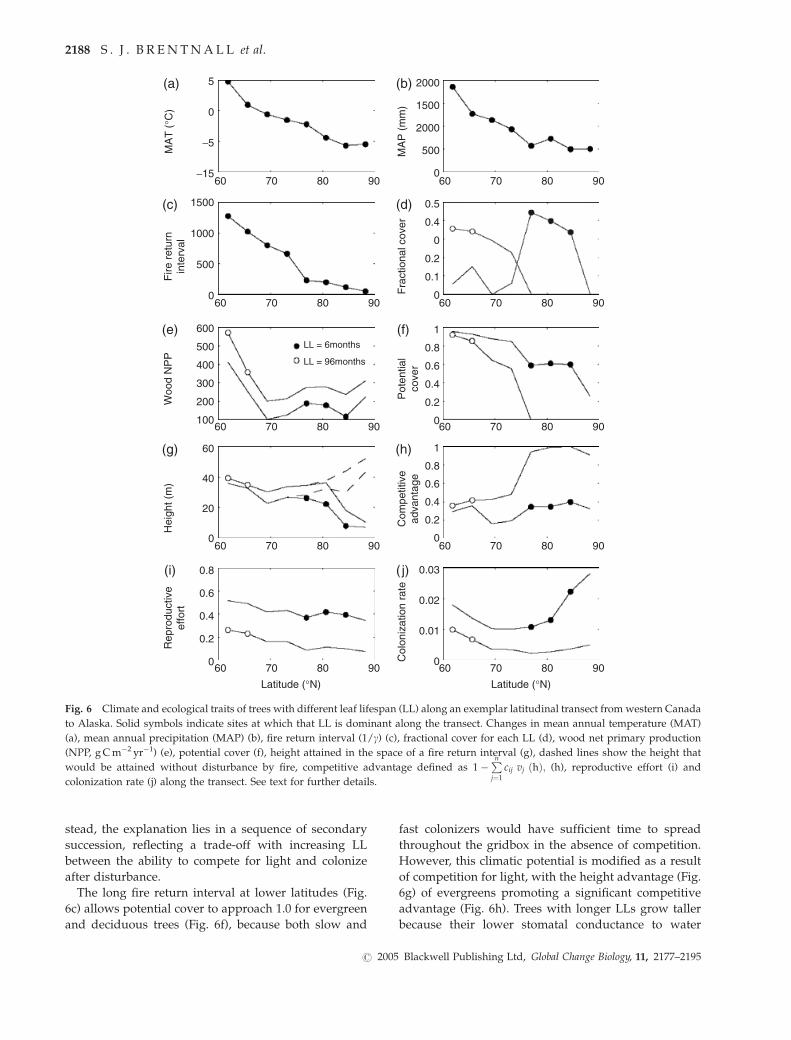
stead, the explanation lies in a sequence of secondary

succession, reflecting a trade-off with increasing LL

between the ability to compete for light and colonize

after disturbance.

The long fire return interval at lower latitudes (Fig.

6c) allows potential cover to approach 1.0 for evergreen

and deciduous trees (Fig. 6f), because both slow and

fast colonizers would have sufficient time to spread

throughout the gridbox in the absence of competition.

However, this climatic potential is modified as a result

of competition for light, with the height advantage (Fig.

6g) of evergreens promoting a significant competitive

advantage (Fig. 6h). Trees with longer LLs grow taller

because their lower stomatal conductance to water

5

0

1500

1000

500

0

600

500

400

300

200

100

60

40

20

0

0.8

0.6

0.4

0.2

0

−5

−15

2000

1500

2000

500

0

0.5

0.4

0

0.2

0.1

0

1

0.8

0.6

0.4

0.2

0

1

0.8

0.6

0.4

0.2

0

0.03

0.02

0.01

0

60 70 80 90 60 70 80 90

60 70 80 90 60 70 80 90

60 70 80 90 60 70 80 90

60 70 80 90 60 70 80 90

60 70 80 90 60 70 80 90

Rep

rodu

ctiv

eef

fort

Col

oniz

atio

n ra

te

Hei

ght (

m)

Com

petit

ive

adva

ntag

e

Woo

d N

PP

Pot

entia

lco

ver

Fire

ret

urn

inte

rval

Fra

ctio

nal c

over

MA

T (

°C)

MA

P (

mm

)

Latitude (°N)Latitude (°N)

LL = 6months

LL = 96months

(a) (b)

(d)(c)

(e)

(g) (h)

(i) ( j)

(f)

Fig. 6 Climate and ecological traits of trees with different leaf lifespan (LL) along an exemplar latitudinal transect from western Canada

to Alaska. Solid symbols indicate sites at which that LL is dominant along the transect. Changes in mean annual temperature (MAT)

(a), mean annual precipitation (MAP) (b), fire return interval (1/g) (c), fractional cover for each LL (d), wood net primary production

(NPP, g C m�2 yr�1) (e), potential cover (f), height attained in the space of a fire return interval (g), dashed lines show the height that

would be attained without disturbance by fire, competitive advantage defined as 1�Pnj¼1

cij vj ðhÞ; (h), reproductive effort (i) and

colonization rate (j) along the transect. See text for further details.



vapour (Reich et al., 1999; Wright et al., 2004) can be

matched by a lower trunk conductance, while still

avoiding desiccation of leaves in the treetop (Whitehead

et al., 1984; Osborne & Beerling, 2002b; Koch et al., 2004).

The low trunk conductance of tall trees results from a

high ratio of length to cross-sectional area in sapwood,

which transports water through the trunk. Simulated

tree heights of 40 m (Fig. 6g) are well within the limits

reached by today’s forests of the humid temperate

climate of western Canada, and entirely compatible

with estimates of 40 m for a fossilized deciduous forest

of Eocene age (Metasequoia sp.) from the Canadian High

Arctic (Williams et al., 2003).

As the fire return interval shortens with increasing

latitude, the potential cover of evergreen trees is greatly

diminished (Fig. 6f) because their reproductive effort is

low relative to deciduous trees (Fig. 6i), and coloniza-

tion rate declines rapidly (Fig. 6j) as a consequence of

this and falling NPP (Fig. 6e). At latitudes of 781N and

higher, the colonization rate of evergreens is insufficient

for recovery after fire disturbance, preventing the estab-

lishment of populations and their persistence at high

latitudes (potential cover 5 0). In effect, deciduous trees

establish more rapidly and effectively than evergreens,

and this is a critical determinant of success in a dis-

turbed environment. We emphasize that the absence of

evergreens with long LL from these deciduous high-

latitude forests does not preclude the occurrence of

evergreens with shorter LL. In fact, forests with a range

of LLs are an emergent property of our dynamic vege-

tation model simulations.

We have focused on fire as the mechanism of dis-

turbance because it is the principal determinant of

boreal and subboreal forest composition in the present

day (Johnson, 1992; Frelich, 2002). Furthermore, evi-

dence of wildfire in the Cretaceous polar forests, in

the form of charcoal, is abundant in the Arctic (e.g.

Falcon-Lang et al., 2004), and has been discovered in the

Antarctic (Eklund et al., 2004). Other sources of distur-

bance could, however, easily be incorporated into the

model.

Simulated and observed LLs of Antarctic and high Arcticpolar forests

We sought to unite model predictions of LL with

observations on fossil wood for two case studies on

high northern (Svalbard in the high Arctic) and south-

ern (Alexander Island on the Antarctic Peninsula) lati-

tude sites. Analysing the fossil remains of polar forests

from these two sites provides information about the

actual range of LL in these ecosystems, as well as a

direct quantitative test of model accuracy. Examination

of the two specific localities shifts the focus from

latitudinal gradients of climate to variation in LL.

From Svalbard, LL values estimated from fossil

woods fell into two distinct groups, with LL either less

(n 5 4) or greater (n 5 8) than 18 months (Table 2). In

comparison, we simulate a bimodal distribution of LLs

at this locality, with peaks of fractional cover at 6

months in the deciduous and 48 months in the ever-

green range (Fig. 7a). This result compares favourably

with the two groups of LL estimated using fossils,

which had mean values of 8 and 50 months, respec-

tively (Table 2; Fig. 7a). Two independent lines of

evidence therefore indicate that Svalbard was popu-

lated by a mixed forest biome in the Early Cretaceous.

On Alexander Island, Antarctica, our reinterpretation

of a published report of PL for a range of wood taxa

(Falcon-Lang & Cantrill, 2000) (Eqn (11)) gives a differ-

ent pattern, with only a single taxon having a short LL,

and four taxa with LL of 79 months or more (Table 2).

The range of high LLs at this site are in agreement with

complementary approaches used to infer leaf habit from

fossils, especially the presence of leaf traces, leaf taph-

onomy and leaf physiognomy (Falcon-Lang & Cantrill,

2000). The wood taxa used in this analysis closely

Table 2 Estimated leaf lifespan (LL � upper and lower 95%

confidence limits) of fossil woods from the European high

Arctic (Svalbard) and Alexander Island, Antarctica

Site Wood taxon

Estimated LL

( � 95% range)

(months)

Svalbard Laricioxylon (species A) 11 (5.5–18.2)

Laricioxylon (species B) 5 (2.1–9.2)

Taxodioxylon (species C) 13 (6.7–21.1)

Protocedroxylon 18 (9.8–27.9)

Mean 11.8 (5.9–19.4)

Araucariopitys 57 (38.7–75.9)

Piceoxylon 35 (21.7–49.6)

Cedroxylon 76 (54.3–97.7)

Xenoxylon 69 (48.5–89.7)

Taxodioxylon 42 (26.9–58.2)

Taxodioxylon

(species B)

100 (75.0–124.5)

Cupressinoxylon 48 (31.6–65.3)

Juniperoxylon 41 (26.2–57.0)

Mean 58.5 (40.0–77.7)

Alexander

Island

Taxodioxylon 13 (6.7–21.1)

Araucarioxylon 83 (60.2–105.6)

Araucariopitys 79 (56.8–101.1)

Podocarpoxylon

(morphospecies 1)

89 (65.4–112.3)

Podocarpoxylon

(morphospecies 2)

98 (73.2122.3)

Mean 87.3 (63.9–110.4)



mirror the foliage fossil record at the same locality

(Cantrill & Falcon-Lang, 2001). Model simulations for

Alexander Island indicate a predominance of evergreen

trees with LL448 months, and a minor component of

deciduous trees with LL 5 9 months (Fig. 7b).

Estimated and simulated LLs from both Arctic and

Antarctic sites are in close quantitative agreement, an

agreement that provides strong validation for the

coupled USCM and forest dynamics scheme. Climatic

differences and ensuing disturbance regimes between

the sites underpin their contrasting forest compositions.

In Svalbard, a cool, dry climate (unadjusted MAT 5

4 1C, MAP 5 600 mm) yields a fire return interval of

80 years, leaving insufficient time for evergreen trees

with long LL to achieve a high potential cover (Fig. 8a,

Eqn (6)) as colonization rate declines sharply with

LL (Fig. 8b). This results from a decrease in the parti-

tioning of resources to reproduction with LL (Fig. 8c,

Eqns (2) and (3)), rather than a change in NPP with LL

(Fig. 8d). Potential cover of deciduous trees with short

LLs is also constrained by colonization rate (Fig. 8a and

b), as a consequence of decreasing reproductive effort

(Fig. 8c) and NPP (Fig. 8d). The net outcome is the

elimination of trees with very short or very long LLs by

fire (Fig. 7a). The most successful trees, in terms of

cover, are those with an LL ensuring they attain reason-

able potential cover while retaining a significant com-

petitive advantage (Fig. 8e). Competitive advantage

mirrors height (Fig. 8f, Eqn (4)), which is inversely

related to the transpiration rate. Transpiration peaks

with an LL of 18 months because the short-lived ever-

green canopy attains both a high LAI in combination

with a high stomatal conductance. The mixture of trees

at this locality reflects the complex interplay between

climate, LL and the ecological processes involved in

succession.

On Alexander Island the warm, wet climate (GCM

MAT 5 6.9 1C, MAP 5 1378 mm) lengthens the fire re-

turn interval to 368 years, ensuring that trees with all

LLs have a high potential cover (Fig. 8a). In support of

such low fire frequencies, we note that long tree ring

sequences of fossil woods from the same Antarctic site

indicate tree longevities of at least 180 years (Chapman,

1994; Falcon-Lang & Cantrill, 2000). Consequently, for-

est composition is determined by competition for light

(Fig. 8e) (i.e. by the potential height of trees with each

LL) (Fig. 8f). Without frequent disturbance, the small

height advantage of slow colonizing trees with long LLs

(448 months) is enough to tip the balance decisively in

their favour, leaving only 10% of the vegetated area

occupied by deciduous trees (Fig. 7b). The marked

contrast in forest composition at this locality with that

at Svalbard highlights the critical importance of vegeta-

tion dynamics for shaping community composition in

the postdisturbance environment. Disturbances other

than fire, such as wind-throw, volcanism, herbivory or

flooding, would amplify these effects.

Conclusion

Palaeobotanical interpretation of polar forests has long

hinged on the assumption that the deciduous leaf habit

was an important adaptation for tree survival in a

warm, high-latitude environment (Osborne et al.,

2004). Recent experiments (Royer et al., 2003, 2005)

and the reinterpretation of Antarctic fossil floras (Fal-

con-Lang & Cantrill, 2001a, b) are now challenging this

view. This paper presents a first attempt at an alter-

native interpretation of the factors controlling the bio-

geography of LL in polar forests that links mechanistic

understanding of its functional consequences for plant

resource-use and forest dynamics. An important out-

come highlighted by our analyses is the crucial influ-

ence of disturbance and its interaction with LL. We

recognize that there are alternative approaches to simu-

lating fire in the natural landscape (e.g. Thonicke et al.,

0.8

0.7

0.6

0.5

0.4

0.3

0.2

0.1

0

Fra

ctio

nal c

over

age

0.8

0.7

0.6

0.5

0.4

0.3

0.2

0.1

0

Fra

ctio

nal c

over

age

0 20 40 60 80 100LL (months)

0 20 40 60 80 100LL (months)

Svalbard Alexander Island

ModelledObservations

(a) (b)

Fig. 7 Modelled and observed dominance of trees with different leaf lifespans (LLs) of the Cretaceous polar conifer forests of Svalbard

(a) and Alexander Island, Antarctica (b). For Svalbard, the mean and range of the observed deciduous LLs are shown; for the evergreens,

the mean and interquartile range is indicated. Individual estimates of LL are shown for Alexander Island.



2001) and to describing the relationship between LL and

the process of succession (e.g. Shugart & Smith, 1996;

Hall & Hollinger, 2000; Bugmann, 2001). Our work,

therefore, represents the first step towards developing

an alternative perspective on the significance that LL

holds for polar forest biogeography.

Acknowledgements

We thank Dana Royer, Ian Woodward, Howard Falcon-Lang andan anonymous reviewer for helpful comments on the manu-script. D. J. B. and J. E. F. gratefully acknowledge funding of thiswork through the NERC (NER/A/S/2001/00435). MH grate-fully acknowledges funding through the NERC studentship(NERC/S/J/2002/10896) and V. W. a Worldwide UniversityNetwork (WUN) research studentship. J. E. F. thanks L. A. Frakes(University of Adelaide) and the Australian Research Council for

the opportunity to collect wood on Svalbard and C. Day for fieldassistance.

References

Amiot R, Lecuyer C, Buffetaut E et al. (2004) Latitudinal tem-

perature gradient during the Cretaceous Upper Campanian-

Middle Maastrichtian: d18O record of continental vertebrates.

Earth and Planetary Science Letters, 226, 255–272.

Archangelsky S (1963) A new Mesozoic flora from Tico, Santa

Cruz province, Argentina. Bulletin of the British Museum (Nat-

ural History), Geology, 8, 47–92.

Axelrod DI (1966) Origin of deciduous and evergreen habits in

temperate forests. Evolution, 20, 1–15.

Axelrod DI (1984) An interpretation of Cretaceous and Tertiary

biota in polar regions. Palaeogeography, Palaeoclimatology, Pa-

laeoecology, 45, 105–147.

1 0.06

0.05

0.04

0.03

0.02

0.01

0

900

800

700

600

500

400

300

200

50

45

40

35

30

25

20

0.9

0.8

0.7

0.6

0.5

0.4

0.3

0.20 20 40 60 80 100 0 20 40 60 80 100

0 20 40 60 80 100 0 20 40 60 80 100

0 20 40 60 80 100 0 20 40 60 80 100

1

0.8

0.6

0.4

0.2

0

0.8

0.7

0.6

0.5

0.4

0.3

0.2

0.1

0

Leaf lifespan (months) Leaf lifespan (months)

Com

petit

ive

adva

ntag

e

Hei

ght (

m)

Rep

rodu

ctiv

e ef

fort

Woo

d N

PP

Pot

entia

l cov

er

Col

oniz

atio

n ra

te

Svalbard

Alexander Island

(a)

(c)

(e) (f)

(b)

(d)

Fig. 8 The simulated influence of leaf lifespan (LL) on the ecological properties of Cretaceous polar forests at Svalbard (European high

Arctic) and Alexander Island, Antarctica. The graphs illustrate the effect of LL on potential cover (a), colonization rate (b), reproductive

effort (c), wood net primary production (NPP, g C m�2 yr�1) (d), competitive advantage (e) and height (f). See text for details.



Barron EJ, Fawcett PJ, Peterson WH et al. (1995) A ‘simulation’ of

the mid-cretaceous. Paleoceanography, 10, 953–962.

Bazzaz FA (1979) The physiological ecology of plant succession.

Annual Review of Ecological Systematics, 10, 351–371.

Bazzaz FA (1996) Plants in Changing Environments. Linking Phy-

siological, Population, and Community Ecology. Cambridge Uni-

versity Press, Cambridge.

Beerling DJ, Osborne CP (2002) Physiological ecology of Meso-

zoic polar forests in a high CO2 environment. Annals of Botany,

89, 329–339.

Beerling DJ, Woodward FI (2001) Vegetation and the Terrestrial

Carbon Cycle. Modelling the First 400 Million Years. Cambridge

University Press, Cambridge.

Boyd A (1994) Some limitations in using leaf physiognomic data as

a precise method for determining palaeoclimates with an ex-

ample from the Late Cretaceous Pautut Flora of West Greenland.

Palaeogeography, Palaeoclimatology, Palaeoecology, 112, 261–278.

Bugmann H (2001) A review of forest gap models. Climatic

Change, 51, 259–305.

Cantrill DJ (1995) The occurrence of a fern Hausmannia Dunker

(Dipteridaceae) in the Cretaceous of Alexander Island, Ant-

arctica. Alcheringa, 19, 243–254.

Cantrill DJ, Falcon-Lang HJ (2001) Cretaceous (Late Albian)

Coniferales of Alexander Island, Antarctica. part 2: leaves,

reproductive organs and roots. Review of Palaeobotany and

Palynology, 115, 119–145.

Chaloner WG, Creber GT (1990) Do fossil plants give a climatic

signal? Journal of the Geological Society, London, 147, 343–350.

Chaney RW (1947) Tertiary centers and migration routes. Ecolo-

gical Monographs, 17, 139–148.

Chanzy A, Bruckler L (1993) Significance of soil surface moisture

with respect to daily bare soil evaporation. Water Resources

Research, 29, 1113–1125.

Chapman JL (1994) Distinguishing internal developmental char-

acteristics from external palaeoenvironmental effects in fossil

wood. Review of Palaeobotany and Palynology, 81, 19–32.

Cox PM (2001) Description of the ‘TRIFFID’ dynamic global vegeta-

tion model. Hadley Centre Technical Note, 24, 16pp.

Crane PR (1987) Vegetational consequences of angiosperm di-

versification. In: The Origins of Angiosperms and their Biological

Consequences (eds Friis EM, Chaloner WG, Crane PR), pp. 107–

144. Cambridge University Press, Cambridge.

Creber GT, Chaloner WG (1984) Influence of environmental

factors on the wood structure of living and fossil trees. The

Botanical Review, 50, 357–448.

Creber GT, Chaloner WG (1985) Tree growth in the Mesozoic and

Early Tertiary and the reconstruction of palaeoclimates. Pa-

laeogeography, Palaeoclimatology, Palaeoecology, 52, 35–60.

Crowley TJ, Berner RA (2001) CO2 and climate change. Science,

292, 870–872.

DeFries R, Hansen M, Townshend JRG et al. (2000a) Continuous

Fields 1 km Tree Cover. The Global Land Cover Facility, College

Park, MD.

DeFries R, Hansen M, Townshend JRG et al. (2000b) A new

global 1 km data set of percent tree cover derived from remote

sensing. Global Change Biology, 6, 247–254.

DePury DGG, Farquhar GD (1997) Simple scaling of photosynth-

esis from leaves to canopies without errors of big-leaf models.

Plant, Cell and Environment, 20, 537–557.

Dettmann ME (1989) Antarctica: Cretaceous cradle of austral

temperate rainforests? Geological Society Special Publication, 42,

89–105.

Dettmann ME, Molnar RE, Douglas JG et al. (1992) Australian

Cretaceous terrestrial fauna and floras: biostratigraphic and

biogeographic implications. Cretaceous Research, 13, 207–262.

Didier L (2001) Invasion patterns of European larch and Swiss

stone pine in subalpine pastures in the French Alps. Forest

Ecology and Management, 145, 67–77.

Dole&al J, Ishii H, Vetrova VP et al. (2004) Tree growth

and competition in a Betula platyphylla-Larix cajanderi post-

fire forest in Central Kamchatka. Annals of Botany, 94,

333–343.

Douglas JG, Williams GE (1982) Southern polar forests: the early

Cretaceous floras of Victoria and their palaeoclimatic signi-

ficance. Palaeogeography, Palaeoclimatology, Palaeoecology, 39,

171–185.

Dungan RJ, Whiteheard D, McGlone M et al. (2004) Simulated

carbon uptake for a canopy of two broadleaved tree species

with contrasting leaf habit. Functional Ecology, 18, 34–42.

Dutton AL, Lohmann KC, Zinsmeister WJ (2002) Stable isotope

and minor element proxies for Eocene climate of Seymour

Island, Antarctica. Paleoceanography, 17, 1016, doi: 10.1029/

2000PA000593.

Eklund HE, Cantrill DJ, Francis JE (2004) Late Cretaceous plant

mesofossils from Table Nunatak, Antarctica. Cretaceous Re-

search, 25, 211–228.

Enquist BJ, Brown JH, West GB (1998) Allometric scaling of plant

energetics and population density. Nature, 395, 163–165.

Farquhar GD, von Caemmerer S, Berry JA (1980) A biochemical

model of photosynthetic CO2 assimilation in leaves of C3

species. Planta, 149, 78–90.

Falcon-Lang HJ (2000a) A method to distinguish between woods

produced by evergreen and deciduous coniferopsids on the

basis of growth ring anatomy: a new palaeoecological tool.

Palaeontology, 43, 785–793.

Falcon-Lang HJ (2000b) The relationship between leaf longevity

and growth ring markedness in modern conifer woods and its

implications for palaeoclimatic studies. Palaeogeography, Pa-

laeoclimatology, Palaeoecology, 160, 317–328.

Falcon-Lang HJ (2005) Intra-tree variability in wood anatomy,

and its implications for fossil wood systematics and palaeocli-

matic datasets. Palaeontology, 48, 171–183.

Falcon-Lang HJ, Cantrill DJ (2000) Cretaceous (Late Albian)

coniferales of Alexander Island, Antarctica: Wood taxonomy:

a quantitative approach. Review of Palaeobotany and Palynology,

111, 1–17.

Falcon-Lang HJ, Cantrill DJ (2001a) Leaf phenology of some mid-

Cretaceous polar forests, Alexander Island, Antarctica. Geolo-

gical Magazine, 138, 39–52.

Falcon-Lang HJ, Cantrill DJ (2001b) Gymnosperm woods

from the Cretaceous (mid-Aptian) Cerro Negro Forma-

tion, Byers Peninsula, Livingston Island, Antarctica: the arbor-

escent vegetation of a volcanic arc. Cretaceous Research, 22,

277–293.

Falcon-Lang HJ, MacRae RA, Csank AZ (2004) Palaeoecology of

Late Cretaceous polar vegetation preserved in the Hansen

Point Volcanics, NW Ellesmere Island, Canada. Palaeogeogra-

phy, Palaeoclimatology, Palaeoecology, 212, 45–64.



Frakes LA, Francis JE (1988) A guide to Phanerozoic cold polar

climates from high-latitude ice-rafting in the Cretaceous. Nat-

ure, 333, 547–549.

Francis JE, Poole I (2002) Cretaceous and early Tertiary climates

of Antarctica: evidence from fossil wood. Palaeogeography,

Palaeoclimatology, Palaeoecology, 182, 47–64.

Frelich LE (2002) Forest Dynamics and Disturbance Regimes. Studies

from Temperate Evergreen–Deciduous Forests. Cambridge Univer-

sity Press, Cambridge.

Givnish TJ (2002) Adaptive significance of evergreen vs. decid-

uous leaves: solving the triple paradox. Silva Fennica, 36,

703–743.

Grime JP (2001) Plant Strategies, Vegetation Processes, and Ecosys-

tem Properties. John Wiley & Sons Ltd, Chichester.

Grubb PJ (2002) Leaf form and function – towards a radical new

approach. New Phytologist, 155, 317–320.

Hall GMJ, Hollinger DY (2000) Simulating New Zealand forest

dynamics with a generalized temperate forest gap model.

Ecological Applications, 10, 115–130.

Harland BM (2005) Cretaceous polar conifer forests: Composi-

tion, leaf life-span and climate significance. PhD thesis, Uni-

versity of Leeds, Leeds, UK.

Hayes PA (1999) Cretaceous angiosperm leaf floras from Antarctica.

PhD thesis, University of Leeds, Leeds.

Herman A (1994) Diversity of the Cretaceous Platanoid plants of

the Anadyr’-Koryak subregion in relation to climatic changes.

Stratigraphy and Geological Correlation, 2, 365–378.

Herman AB, Spicer RA (1996) Palaeobotanical evidence for a

warm Cretaceous Arctic ocean. Nature, 380, 330–333.

Hewitt CD, Mitchell JFB (1996) GCM simulations of the climate

of 6 kyr BP: mean changes and interdecadal variability. Journal

of Climate, 9, 3505–3529.

Hickey LJ (1984) Eternal summer at 80 degrees north. Discovery,

17, 17–23.

Hill RS, Scriven LJ (1995) The angiosperm–dominated woody

vegetation of Antarctica – a review. Review of Palaeobotany and

Palynology, 86, 175–198.

Hollinger DY (1992) Leaf and simulated whole-canopy photo-

synthesis in 2 co-occurring tree species. Ecology, 73, 1–14.

Hotinski RM, Toggweiler JR (2003) Impact of a Tethyan circum-

global passage on ocean heat transport and ‘equable’ climates.

Paleoceanography, 18 doi:10.1029/2001PA000703.

Jain TB, Graham RT, Morgan P (2004) Western white pine growth

relative to forest openings. Canadian Journal of Forest Research,

34, 2187–2198.

Jenkyns HC, Forster A, Schouten S et al. (2004) High latitude

temperatures in the Late Cretaceous. Nature, 432, 888–892.

Johnson EA (1992) Fire and Vegetation Dynamics: Studies from the

North American Boreal Forest. Cambridge University Press,

Cambridge.

Kennedy EM, Spicer RA, Rees PM (2002) Quantitative paleocli-

mate estimates from Late Cretaceous and Paleocene leaf floras

in the northwest of South Island, New Zealand. Palaeogeogra-


Kikuzawa K (1991) A cost–benefit analysis of leaf habit and leaf

longevity of trees and their geographical pattern. American

Naturalist, 138, 1250–1263.

Koch GW, Sillett SC, Jennings GM et al. (2004) The limits to tree

height. Nature, 428, 851–854.

Leuning R (1995) A critical appraisal of a combined stomatal-

photosynthesis model for C3 plants. Plant, Cell and Environ-

ment, 18, 339–355.

Markwick PJ (1998) Fossil crocodilians as indicators of Late

Cretaceous and Cenozoic climates: implications for using

palaeontological data in reconstructing palaeoclimate. Palaeo-

geography, Palaeoclimatology, Palaeoecology, 137, 205–271.

Margolis H, Oren R, Whitehead D et al. (1995) Leaf area

dynamics of conifer forests. In: Ecophysiology of Coniferous

Forests (eds Smith WK, Hinkley TM), pp. 181–223. Academic

Press, San Diego.

Mason HL (1947) Evolution of certain floristic associations in

Western North America. Ecological Monographs, 17, 201–210.

Meeson BW, Corprew FE, McManus JM et al. (1995) The ISLSCP

Initiative I – Global Datasets for Land-Atmosphere Models, 1987–

1988. Volumes 1–5 published on CD by NASA.

Monteith JL (1965) Evaporation and the environment. In: The

State and Movement of Water in Living Organisms (ed Fogg CE),

pp. 205–234. Cambridge University Press, New York.

Myneni RB, Nemani RR, Running SW (1997) Estimation of global

leaf area index and absorped PAR using radiative transfer

models. IEEE Transactions on Geoscience and Remote Sensing, 35,

1380–1393.

New M, Hulme M, Jones PD (1999) Representing twentieth

century space-time climate variability. I. Development of a

1961–90 mean monthly terrestrial climatology. Journal of Cli-

mate, 12, 829–856.

New M, Hulme M, Jones PD (2000) Representing twentieth

century space–time climate variability. II. Development of

1901–96 mean monthly grids of terrestrial surface climate.

Journal of Climate, 13, 2217–2238.

Osborne CP, Beerling DJ (2002a) A process-based model of

conifer forest structure and function with special emphasis

on leaf lifespan. Global Biogeochemical Cycles, 16, 1097,

doi:10.1029/2001GB001467 (2002).

Osborne CP, Beerling DJ (2002b) Sensitivity of tree growth to a

high CO2 environment: consequences for interpreting the

characteristics of fossil woods from ancient ‘greenhouse’

worlds. Palaeogeography, Palaeoclimatology, Palaeoecology, 182,

15–29.

Osborne CP, Beerling DJ (2003) The penalty of a long hot summer.

Photosynthetic acclimation to high CO2 and continuous light in

‘living fossil’ conifers. Plant Physiology, 133, 803–812.

Osborne CP, Royer DL, Beerling DJ (2004) Adaptive role of leaf

habit in extinct polar forests. International Forestry Review, 6,

181–186.

Parrish JT, Spicer RA, Douglas JG et al. (1991) Continental climate

near the Albian South Pole and comparison with the climate

near the North Pole. Geological Society of America Abstracts with

Programs, 23, 31–34.

Parrish JT, Daniel IL, Kennedy EM (1998) Paleoclimatic signifi-

cance of mid-Cretaceous floras from the Middle Clarence

Valley, New Zealand. Palaios, 13, 149–159.

Parton WJ, Scurlock JMO, Ojima DS et al. (1993) Observations

and modelling of biomass and soil organic matter dynamics

for the grassland biome worldwide. Global Biogeochemical

Cycles, 7, 785–809.

Penman HL (1948) Evaporation from open water, bare soil and

grass. Proceedings of the Royal Society, Series A, 193, 120–145.



Pole M, Douglas B (1999) Plant megafossils of the Upper Cretac-

eous Kaitangata coalfield, New Zealand. Australian Systematic

Botany, 12, 331–364.

Pope VD, Gallani ML, Rowntree PR et al. (2000) The impact of

new physical parametrizations in the Hadley Centre climate

model: HadAM3. Climate Dynamics, 16, 123–146.

Read J, Francis J (1992) Responses of some Southern Hemisphere

tree species to a prolonged dark period and their implications

for high-latitude Cretaceous and Tertiary floras. Palaeogeogra-


Reich PB, Ellsworth DS, Walters MB (1998) Leaf structure (spe-

cific leaf area) modulates photosynthesis–nitrogen relations:

evidence from within and across species and functional

groups. Functional Ecology, 12, 948–958.

Reich PB, Ellsworth DS, Walters MB et al. (1999) Generality of

leaf trait relationships: a test across six biomes. Ecology, 80,

1955–1969.

Reich PB, Walters MB, Ellsworth DS (1997) From tropics to

tundra: global convergence in plant functioning. Proceedings

of the National Academy of Sciences, USA, 94, 13730–13734.

Royer DL, Berner RA, Montanez IP et al. (2004) CO2 as a primary

driver of Phanerozoic climate. Geological Society of America

Today, 14, 4–10.

Royer DL, Osborne CP, Beerling DJ (2003) Carbon loss by

deciduous trees in a CO2-rich ancient polar environment.

Nature, 424, 60–62.

Royer DL, Osborne CP, Beerling DJ (2005) Contrasting seasonal

patterns of carbon gain in evergreen and deciduous trees of

ancient polar forests. Paleobiology, 31, 141–150.

Ryan MG, Hubbard RM, Pongracic S et al. (1996) Foliage, fine-

root, woody-tissue and stand respiration in Pinus radiata in

relation to nitrogen status. Tree Physiology, 16, 333–343.

Schmidt GA, Mysak LA (1996) Can increased poleward oceanic

heat flux explain the warm Cretaceous climate? Paleoceanogra-

phy, 11, 579–593.

Schulze E-D, Vygodskaya NN, Tchebakova et al. (2002) The

Eurosiberian Transect: an introduction to the experimental

region. Tellus B, 54, 421–428.

Seward AC (1926) The Cretaceous plant-bearing rocks of Wes-

tern Greenland. Philosophical Transactions of the Royal Society

London, B215, 57–172.

Shaw RH, Pereira AR (1982) Aerodynamic roughness of a plant

canopy: a numerical experiment. Agricultural and Forestry

Meteorology, 26, 51–65.

Shugart HH, Smith TM (1996) A review of forest patch models

and their application to global change research. Climatic

Change, 34, 131–153.

Silvertown J, Lovett-Doust J (1993) Introduction to Plant Popula-

tion Ecology. Blackwell Science, Oxford.

Smiley C (1976) Pre-Tertiary phytogeography and continental

drift – some apparent discrepancies. In: Historical Biogeography,

Plate Tectonics and the Changing Environment (eds Gray J, Boucot

AJ), pp. 311–320. Oregon State University Press, Corvallis,

Oregon.

Smith AG, Smith DG, Funnell BM (1994) Atlas of Mesozoic and

Cenozoic Coastlines. Cambridge University Press, Cambridge.

Spicer RA, Chapman JL (1990) Climate change and the evolution

of high-latitude terrestrial vegetation and flora. Trends in

Ecology and Evolution, 5, 279–284.

Spicer RA, Corfield RM (1992) A review of terrestrial and marine

climates in the Cretaceous with implications for modelling the

‘Greenhouse Earth’. Geological Magazine, 129, 169–180.

Spicer RA, Parrish JT (1986) Palaeobotanical evidence for cool

north polar climates in middle Cretaceous (Albian-Cenoma-

nian) time. Geology, 14, 703–706.

Tarduno JA, Brinkman DB, Renne PR et al. (1998) Evidence for

extreme climatic warmth from Late Cretaceous arctic verte-

brates. Science, 282, 2241–2244.

Thonicke K, Venevsky S, Sitch S et al. (2001) The role of fire

disturbance for global vegetation dynamics: coupling fire into

a dynamic global vegetation model. Global Ecology and Biogeo-

graphy, 10, 661–677.

Tripati A, Zachos J, Marincovich L et al. (2001) Late Paleocene

Arctic coastal climate inferred from molluscan stable and

radiogenic isotope ratios. Palaeogeography, Palaeoclimatology,

Palaeoecology, 170, 101–113.

Upchurch GR, Askin RA (1989) Latest Cretaceous and earliest

Tertiary dispersed cuticles from Seymour Island, Antarctica.

Antarctic Journal of the United States, 24, 7–10.

Upchurch GR, Wolfe JA (1993) Cretaceous vegetation of the

Western Interior and adjacent regions of North America.

Geological Association of Canada Special Paper, 39, 243–281.

Upchurch GR, Otto-Bliesner BL, Scotese CR (1999) Terrestrial

vegetation and its effects on climate during the latest Cretac-

eous. Geological Society of America Special Paper, 332, 407–426.

Valdes PJ, Sellwood BW, Price GD (1996) Evaluating concepts of

Cretaceous equability. Palaeoclimates, 1, 139–159.

Weiss A, Norman JM (1985) Partitioning solar radiation into

direct and diffuse, visible and near-infrared components.

Agricultural and Forestry Meteorology, 34, 205–213.

Whitehead D, Edwards WRN, Jarvis PG (1984) Conducting

sapwood area, foliage area, and permeability in mature trees

of Picea sitchensis, and Pinus contorta. Canadian Journal of

Forestry Research, 14, 940–947.

Williams CJ, Johnson AH, LePage BA et al. (2003) Reconstruction

of Tertiary Metasequoia forests II. Structure, biomass, and

productivity of Eocene floodplain forests in the Canadian high

arctic. Paleobiology, 29, 271–292.

Wolfe JA (1985) Distribution of major vegetation types during

the Tertiary. In: The Carbon Cycle and Atmospheric CO2: Natural

Variations, Archean to Present. Geophysical Monograph Series, Vol.

32. (eds Sundquist ET, Broecker WS), pp. 357–375. American

Geophysical Union, Washington.

Wolfe JA, Upchurch GR (1987) North American nonmarine

climates and vegetation during the Late Cretaceous. Palaeogeo-

graphy, Palaeoclimatology, Palaeoecology, 61, 33–77.

Woodward FI, Lomas MR, Lee SE (2001) Predicting the future

productivity and distribution of global vegetation. In: Terres-

trial Global Productivity (eds Jacques R, Saugier B, Mooney H),

pp. 521–541. Academic Press, New York.

Woodward FI, Smith TM (1994) Global photosynthesis and

stomatal conductance: modelling controls by soils and cli-

mates. Advances in Botanical Research, 20, 1–41.

Woodward FI, Smith TM, Emanuel WR (1995) A global land

primary productivity and phytogeography model. Global Bio-

geochemical Cycles, 9, 471–490.

Wright IJ, Reich PB, Westoby M et al. (2004) The worldwide leaf

economics spectrum. Nature, 428, 821–827.



Appendix A: Validation of coupled USCM

We tested the accuracy of annual LAI and NPP simula-

tions using a database of modern observations encom-

passing a diverse range of LLs (4–138 months), and

climatic regimes ranging from the Russian boreal zone

to the Mediterranean, and Alaska to Florida (Osborne &

Beerling, 2002a). We forced the model with site-average

climatologies for the years 1961–1990 (New et al., 1999,

2000), as LL41 at the majority of test sites, implying the

integration of interannual climate variability by canopy

structure. In all simulations, the USCM was driven with

a mean LL value for the dominant species at each site,

and an atmospheric CO2 concentration appropriate for

the year of observation.

Simulations of LAI for conifer forests at 16 different

sites, and NPP for 23 sites, both give reasonable agree-

ment with observations (Appendix Fig. 1A, LAI

r2 5 0.84, Po0.01, NPP r2 5 0.89, Po0.01). In both cases,

agreement between the USCM and observations was

comparable with that obtained by driving the un-

coupled model with prescribed soil carbon and nitrogen

values (LAI, r2 5 0.88; NPP, r2 5 0.91) (Osborne & Beer-

ling, 2002a), suggesting adequate simulation of soil

carbon and nitrogen cycling in a self-consistent manner.

On a site-by-site basis, therefore, these results indicate

the capability of the USCM to accurately simulate the

structure and function of conifer forests across a wide

climatic gradient from inputs of climate, LL and CO2.

We verified regional-scale model simulations of forest

properties by comparison with satellite data products:

the ISLSCP global land cover dataset (Meeson et al.,

1995), which classifies each 11 gridbox into one of 15

land surface types (water, ice, desert and 12 vegetation

types); the Moderate Resolution Imaging Spectroradi-

ometer monthly 16 km LAI dataset (Myneni et al., 1997),

averaged over the same decade (1982–1991) as the cli-

matological forcing data; the Global Land Cover Facility

tree cover dataset (DeFries et al., 2000a, b); and a 1 km

resolution NPP dataset for 1999 derived from SPOT-

VEGETATION satellite measurements using the C-Fix

methodology (http://www.geosuccess.net). LAI, NPP

and tree cover data were extracted using the ISLSCP

categorization for conifer forests only, and classified as

either evergreen or deciduous. Modelled LAI and NPP

values were weighted by the fractional cover of each LL.

Across all sites (n 5 237) modelled LAI data exceeded

the satellite data by an average of 1.6 (m2 m�2), with a

standard deviation of the differences of 1.9. The agree-

ment is reasonable given the test is imperfect because of

the introduction of errors by methodological proce-

dures for processing satellite data (Beerling & Wood-

ward, 2001). Fractional tree cover also introduced

another source of error. Satellites measure the LAI for

a grid cell that may contain a mixture of vegetation

some of which has a lower LAI than forest (e.g. grass-

land or tundra) or bare ground. Correcting for this effect

using tree cover fraction, assuming an typical LAI for

grasslands/tundra of 2.0, gives a mean error between

observed and modelled of 0.18 with a standard devia-

tion of 0.74; both datasets were significantly correlated

(r2 5 0.34, Po0.001). A Kolmogorov–Smirnov test the

5% significance level showed that the frequency histo-

gram of LAI errors was normally distributed. Overall,

this analysis indicates there was no systematic bias in

simulated forest LAIs at the regional scale.

Across all sites (n 5 237) modelled and satellite NPP

differed by an average of �0.3 g C m�2 yr�1 and a stan-

dard deviation of 158.2 g C m�2 yr�1. This is a reasonable

match given the large difference between the methods

used to estimate NPP. Both datasets were significantly

correlated (r2 5 0.30, Po0.001). A Kolmogorov–Smirnov

test at the 5% significance level showed the frequency

histogram of differences between observed and simulated

lacked systematic bias and were normally distributed.

9

8

7

6

5

4

3

2

1

00 1 2 3 4 5 6 7 8 9 0 200 400 600 800 1000 1200 1400 1600

1600

1400

1200

1000

800

600

400

200

0

Sim

ulat

ed L

AI (

m2

m−2

)

Sim

ulat

ed N

PP

(g

C m

−2 y

r−1)

Observed LAI (m2 m−2) Observed NPP (g C m−2 yr−1)

Fig. A1 Correlations between observed and measured leaf area indices (a) and net primary production of contemporary conifer forests

across a wide climatic gradient. Regression details for (a) r2 5 0.84, Po0.01; and for (b) r2 5 0.89, Po0.01. See Osborne & Beerling (2002a)

for dominant LLs and climatic details of sites.



climatic and ecological determinants of leaf lifespan in ... · pdf filepolar forests once...

Documents