K.S. Kavi Kumar

MADRAS SCHOOL OF ECONOMICSGandhi Mandapam Road

Chennai 600 025 India

April 2009

CLIMATE SENSITIVITY OF INDIAN AGRICULTURE

WORKING PAPER 43/2009

Climate Sensitivity of Indian Agriculture

K.S. Kavi Kumar Email : kavi@mse.ac.in; kavikumar@gmail.com

WORKING PAPER 43/2009

April 2009

Price : Rs. 35

MADRAS SCHOOL OF ECONOMICS

Gandhi Mandapam Road Chennai 600 025

India

Phone: 2230 0304/ 2230 0307/2235 2157

Fax : 2235 4847 /2235 2155

Email : info@mse.ac.in

Website: www.mse.ac.in

Climate Sensitivity of Indian Agriculture

K.S. Kavi Kumar

Abstract

Climate change impact studies on agriculture are broadly based on agronomic-economic approach and Ricardian approach. The Ricardian approach, similar in principle to the Hedonic pricing approach of environmental valuation, has received significant attention due to its elegance and also some strong assumptions it makes. This paper attempts to extend the existing knowledge in this field by specifically addressing two important issues: (a) extent of change in climate sensitivity of Indian agriculture over time; (b) importance of accounting for spatial features in the assessment of climate sensitivity. The analysis based on four decades of data suggests that the climate sensitivity of Indian agriculture is increasing over time, particularly in the period from mid-eighties to late nineties. This finding corroborates the growing evidence of weakening agricultural productivity over the similar period in India. The results also show presence of significant positive spatial autocorrelation, necessitating estimation of climate sensitivity while controlling for the same. While many explanations may exist for the presence of spatial autocorrelation, this paper argued that inter-farmer communication could be one of the primary reasons for the spatial dependence. Field studies carried out in Andhra Pradesh and Tamil Nadu through focus group discussions provided limited evidence in this direction. Key Words: Climate Change; Indian Agriculture; Environmental Valuation; Spatial Econometrics; Adaptation JEL Codes: Q54, Q1, R1

Acknowledgements This paper is presented at IV Congress of the Latin American and

Caribbean Association of Environmental and Natural Resource Economics,

Universidad Nacional, Heredia, Costa Rica, 19-21 March 2009. The author

would like to thank the conference participants for useful comments; and

Brinda Viswanathan and Jaya Krishnakumar for helpful suggestions on

spatial econometric work. The financial support provided by South Asian

Network for Environment and Development Economics (SANDEE) is

gratefully acknowledged.

1

1. INTRODUCTION

Over the past two decades the debate on global climate change has

moved from scientific circles to policy circles with the world nations more

seriously than ever exploring a range of response strategies to deal with

this complex phenomenon that is threatening to have significant and far

reaching impacts on human society. The Intergovernmental Panel on

Climate Change (IPCC) in its fourth assessment report observed that,

„warming of climate system is now unequivocal, as is now evident from

observations of increases in global average air and ocean temperatures,

widespread melting of snow and ice, and rising global sea level‟ (Solomon

et al., 2007). Policy responses to climate change include mitigation of

GHGs that contribute to the expected changes in the Earth‟s climate, and

adaptation to potential impacts caused by the changing climate. While

the first one is largely seen as a reactive response to climate change, the

second one is a proactive response. Though GHG mitigation policies have

dominated the overall climate policy so far, adaptation strategies are also

being emphasized now to form a more comprehensive policy response.

The United Nations Framework Convention on Climate Change

(UNFCCC) – the international apex body on climate change – refers to

adaptation in the context of change in climate only. In other words

without greenhouse gas emissions there is no climate change and hence

no need for adaptation. Going by this widely accepted interpretation,

adaptation is necessary only because mitigation of greenhouse gases

may not completely halt climate change. Stern Review summarizes this

view: „adaptation is crucial to deal with the unavoidable impacts of

climate change to which the world is already committed‟ (Stern, 2006,

emphasis added).

For both mitigation and adaptation policy formulation, one of the

crucial inputs needed is the potential impacts due to climate change on

various climate sensitive sectors. For mitigation, such information would

2

provide the required justification for de-carbonizing the energy systems.

On the other hand, in the context of adaptation, knowledge on climate

change induced impacts will be helpful in prioritizing the adaptation in

the most needed sectors and regions. Further, climate change impacts

estimated with proper accounting of adaptation will be helpful in

identifying the factors that ameliorate the adverse effects of climate

change.

1.1 Climate Change and Indian Agriculture

With more than sixty percent of its population dependent on climate

sensitive activities such as agriculture, the impacts of climate change on

agriculture assume significant importance for India. Climate change

projections made up to 2100 for India, indicate an overall increase in

temperature by 2-4oC coupled with increase in precipitation, especially

during the monsoon period. Mall et al. (2006) provide an excellent review

of climate change impact studies on Indian agriculture mainly from

physical impacts perspective. The available evidence shows significant

drop in yields of important cereal crops like rice and wheat under climate

change conditions. However, biophysical impacts on some of the

important crops like sugarcane, cotton and sunflower have not been

studied adequately.

The economic impacts of climate change on agriculture have

been studied extensively world over and it continues to be a hotly

debated research problem. Two broad approaches have been used so far

in the literature to estimate the impact of climate change on agriculture:

(a) Agronomic-economic approach that focuses on structural modeling of

crop and farmer response, combining the agronomic response of

plants with economic/management decisions of farmers. This

approach is also referred as Crop Modeling approach and Production

Function approach;

3

(b) Spatial analogue approach that exploits observed differences in

agricultural production and climate among different regions to

estimate a climate response function. This approach is referred as

Ricardian approach and is similar in spirit to hedonic pricing

technique of environmental valuation.

In the first approach the physical impacts (in the form of yield

changes and/or area changes estimated through crop simulation models)

are introduced into an economic model exogenously as Hicks neutral

technical changes. In the Indian context Kumar and Parikh (2001a)

showed that under doubled carbon dioxide concentration levels in the

later half of twenty first century the gross domestic product would

decline by 1.4 to 3 percentage points under various climate change

scenarios. More significantly they also estimated increase in the

proportion of population in the bottom income groups of the society in

both rural and urban India under climate change conditions. While this

approach can account for the so-called carbon fertilization effects1, one

of the major limitations is its treatment of adaptation. Since the physical

impacts of agriculture are to be re-estimated under each adaptation

strategy, only a limited number of strategies can be analyzed.

In an alternative approach, called Ricardian approach,

Mendelsohn et al. (1994) have attempted to link land values to climate

through reduced-form econometric models using cross-sectional

evidence. This approach is similar to Hedonic pricing approach of

environmental valuation. Since this approach is based on the observed

evidence of farmer behavior it could „in principle‟ include all adaptation

possibilities. Of course, if the predicted climate change is much larger

than the observed climatic differences across the cross-sectional units

1 Higher carbon dioxide concentrations in the atmosphere under the climate

change conditions could act like aerial fertilizers and boost the crop growth.

This phenomenon is called carbon fertilization effect.

4

then the Ricardian approach can not (even in principle) fully account for

adaptation.

While the Ricardian approach has the potential for addressing the

adaptation satisfactorily, the issues concerning the cost of adaptation are

not completely addressed. One of the main concerns of this approach is

that it may confound climate with other unobserved factors. Recently,

Deschenes and Greenstone (2005) and Schlenker and Roberts (2008)

among others, have addressed this issue. Further, the constant relative

prices assumption used in this approach could bias the estimates (see,

Cline, 1996; Darwin, 1999; Quiggin and Horowitz, 1999 for a critique on

this approach). For India, Kumar and Parikh (2001b) and Sanghi and

Mendelsohn (2008) have used a variant of this approach and showed

that a 2oC temperature rise and seven percent increase in rainfall would

lead to almost 10 percent loss in farm level net revenue (1990 net-

revenue). The regional differences are significantly large with northern

and central Indian districts along with coastal districts bearing relatively

large impact. Mendelsohn et al. (2001) have compared climate sensitivity

of the US, Brazilian and Indian agriculture using the estimates based on

the Ricardian approach and have argued that using the US estimates for

assessing climate change impacts on Indian agriculture would lead to

under-estimation of impacts.

The results of the two broad approaches outlined above

correspond to what could be termed as „typical‟ and „clairvoyant‟ farmer,

respectively. While the estimates from agronomic-economic approach

account for adaptation only in partial manner, the Ricardian approach

treats farmer as though she has perfect foresight. In the Ricardian

approach farmers are assumed to identify instantaneously and perfectly

any change in climate, evaluate all associated changes in market

conditions and then modify their actions to maximize profits. These

assumptions also imply that agricultural system is ergodic – i.e., space

and time are substitutable. Ergodic assumption imply, for example, that

5

skills, institutional and financial endowments for responding to say,

drought (that are typically refined in arid places) are assumed to be

available for use by people in humid areas (where such resources are

under-developed) immediately and in essentially cost-less manner.

Further there is scope for inter-farmer communication and information

diffusion. Both these factors motivate incorporation of spatial features in

the Ricaridan analysis. There are other motivations for accounting for

spatial autocorrelation in the Ricardian analysis. Scope for spatial

autocorrelation of error terms could lead to inefficient estimation of the

coefficients. Recent evidence from the US suggests that either way it is

important to account for spatial autocorrelation to get accurate estimates

of climate sensitivity of agriculture (Polsky, 2004; Schlenker et al., 2006).

Similarly, careful analysis of the changing nature of climate

sensitivity of Indian agriculture is important to understand the role of

technology in ameliorating the climate change impacts. This paper

attempts to incorporate these features into the Ricardian approach to

assess the climate change impacts on Indian agriculture. These also form

the objectives of the paper. The rest of the paper is structured as

follows: The next section explains the model structure and data. The

third section presents results and discusses the distributional issues of

climate change impacts on Indian agriculture. The fourth section briefly

discusses the lessons learned about inter-farmer communication through

focus group meetings in Andhra Pradesh and Tamil Nadu. Finally, the last

section concludes the paper.

2. MODEL SPECIFICATION AND DATA

While the original Ricardian approach developed by Mendelsohn

et al. (1994) estimated relationship between land values and climate, due

to non-existent and/or absence of well functioning land markets in the

developing countries, a variant of Ricardian approach has been used in

6

the earlier Indian studies (see, Dinar et al., 1998). In place of land

values, farm level net-revenue is used as welfare indicator and the value

of the change in the environment is assessed through change in farm

level net revenue. The Ricardian model is thus specified as follows:

),,,,,

,,,,,,,,( 22

ALTIRRHYVCULTIVLITPROPPOPDEN

TRACTORBULLOCKSOILRTRRTTfNR jjjjjj …(1)

where, NR represents farm level net revenue per hectare in constant

rupees; T and R represent temperature and rainfall respectively

(subscript j denotes the season). It may be noted that based on the

existing literature a quadratic functional specification is adopted along

with climate interaction terms. The control variables include soil

(captured through dummies representing several soil texture classes and

top-soil depth classes; represented as SOIL in equation (1)), extent of

mechanization (captured through number of bullocks and tractors per

hectare; represented as BULLOCK and TRACTOR in equation (1)),

percentage of literate population (LITPROP in equation (1)), population

density (POPDEN in equation (1)), altitude (to account for solar radiation

received; ALT in equation (1)), number of cultivators (since the cost of

own labor could not be accounted for while calculating the dependent

variable; CULTIV in equation (1)), fraction of area under irrigation and

fraction of area under high-yielding variety seeds (IRR and HYV,

respectively in equation (1)).

Cross-sectional data is used for estimating the above model.

Districts are the lowest administrative unit at which reliable agricultural

data is available in India. A comprehensive district level dataset of the

period 1956 to 1999 is developed for the purpose of analysis. Agricultural

data at district level is assembled in the dataset along with relevant

demographic and macro economic data. This dataset expands an earlier

dataset developed by the author along with two other researchers for the

period 1956 to 1986 and used in Dinar et al. (1998). The dataset covers

271 districts defined as per 1961 census across thirteen major states of

7

India (Andhra Pradesh, Haryana, Madhya Pradesh, Maharashtra,

Karnataka, Punjab, Tamil Nadu, Uttar Pradesh, Bihar, Gujarat, Rajasthan,

Orissa and West Bengal).

The variables covered in the dataset include, gross and net

cropped area; gross and net irrigated area; cultivators; agricultural

laborers; cropped area under high-yielding variety seeds; total cropped

area under five major crops (rice, wheat, maize, bajra and jowar) and

fifteen minor crops (barley, gram, ragi, tur, potato, ground nut, tobacco,

sesamum, ramseed, sugarcane, cotton, other pulses, jute, soybean, and

sunflower); bullocks; tractors; literacy rate; population density; fertilizer

consumption (N, P, K) and prices; agricultural wages; crop produce; farm

harvest prices; soil texture and top soil depth. For the purpose of analysis

farm level net revenue per hectare is defined as follows:

AreaTotal

CostsLaborandFertilizervenueGrosshapervenueNet

)()Re(Re

…(2)

where, gross revenue is calculated over twenty crops mentioned above,

total area is the cropped area under the twenty crops, fertilizer costs are

total yearly costs incurred towards use of fertilizer for all the crops and

labor costs are yearly expenses towards hiring agricultural laborers. It

may be noted that costs attributable to cultivators, irrigation, bullocks

and tractors are not included in the net revenue calculations as

appropriate prices are difficult to identify. However these variables are

used as control variables in the model as specified in equation (1).

Unfortunately there is no „clean‟ climate data available for the

analysis. Meteorological data is typically collected at meteorological

stations and any district may have one or many stations with in its

boundary. Since all other data is attributable to a hypothetical centre of

the district, the climate data should also be worked out at the centre of

the district. For this purpose meteorological station data is interpolated to

arrive at district specific climate (see, Kumar and Parikh, 2001b and Dinar

8

et al., 1998 for more details on the surface interpolation employed to

generate district level climate data). Climate data corresponding to about

391 meteorological stations spread across India is used for the purpose

of developing district level climate. The data on climate – at the

meteorological stations and hence at the districts – corresponds to

average of observed weather over the period 1951-1980 and is sourced

from a recent publication of India Meteorological Department. All the

climate variables are represented through four months – January, April,

July and October, corresponding to the four seasons. The climate

variables include daily mean temperature and monthly total rainfall.

For the purpose of analysis the dataset is divided into three

distinct periods of almost equal length: 1956-1970; 1971-1985; 1986-

1999. These periods roughly correspond to the pre-green revolution,

green-revolution, and post-green revolution periods of Indian agriculture.

Analysis over these three periods is expected to provide insight on

changing nature of climate sensitivity of Indian agriculture over time. In

each case the panel data is analyzed with year fixed effects2. Fixed and

random year effects specification is tested through Hausman test in each

case. In each time period, Hausman test rejected the null hypothesis,

implying that the random effects model produces biased estimates.

Hence, the fixed effects estimators are preferred. Further, since the units

of analysis (i.e., districts) differ significantly in size and agricultural

activities, the measurement errors might also substantially differ across

districts. Hence the data for each unit of analysis is weighted by the total

area under the twenty crops.

2 It may be noted that district fixed effects are not considered as the climate

data is invariant over time and hence such specification would knock out the

climate coefficients.

9

2.1 Climate Sensitivity and Spatial Autocorrelation

As argued in the first section presence of spatial autocorrelation

necessitates re-specification of model as either spatial lag or spatial error

model as shown below:

Spatial error model: y = X + , where = W + …(3a)

Spatial lag model: y = Wy + X + ...(3b)

where, y is (nx1) vector of dependent variable observations, X is (nxm)

matrix of observations on independent variables including the climate and

other control variables, is (mx1) regression coefficient vector, is (nx1)

vector of spatially correlated error terms, is (1x1) the spatial

autoregressive parameter, W is (nxn) spatial weights matrix, is (nx1)

vector of random error terms. Note that y and X are respectively, the left

hand and right hand side variables specified in equation (1) above. The

period 1966-1986 is considered for the spatial analysis.

One of the crucial inputs needed for spatial analysis is the weight

matrix W. While there are several ways to generate the weight matrix,

the present analysis used rook contiguity based weight matrix generated

for the Indian districts in GeoDa software3. Since it is not feasible to

estimate the spatial fixed effects model in GeoDa, the weight matrix is

transferred via R-software to ASCII data format. The spatial panel model

is estimated using MATLAB software4 for computational efficiency

through the use of sparse matrices. Table 1 summarizes the details of

various analyses carried out.

3 Spatial econometric software developed by Prof. Luc Anselin of University of

Illinois (version 0.9.5).

4 The MATLAB codes for spatial panel analysis are written by J. Paul Elhorst

(www.spatial-econometrics.com).

10

Table 1: Details of Various Analyses

Aim of the Analysis

Period(s) of Analysis

Model Specification

Estimation Procedure and Software Used

Explore changing nature of climate sensitivity over time

1956-1999 with sub-periods: 1956-1970;

1971-1985; 1986-1999

Equation (1) Panel fixed (year) effects by weighting the observations; STATA 9.2

Explore influence of spatial autocorrelation on climate sensitivity

1966-1986 Equation (3a) and (3b)

Panel fixed (year) effects with correction for spatial autocorrelation; GeoDA; R; MATLAB 7

2.2 Climate Change Projections for India

The climate change projections for India used for the analysis are those

reported in Cline (2007). The climate change projections are average of

predictions of six general circulation models including HadCM3, CSIRO-

Mk2, CGCM2, GFDL-R30, CCSR/NIES, and ECHAM4/OPYC3. Table 2

shows the region-wise and season-wise temperature and rainfall changes

for the period 2070-2099 with reference to the base period 1960-1990.

From these regional projections, state-wise climate change predictions

are assessed by comparing the latitude-longitude ranges of the regions

with those of the states. Besides this India specific climate change

scenario, the impacts are also assessed for two illustrative uniform

climate change scenarios (+2oC temperature change along with +7

percent precipitation change; and +3.5oC temperature change along with

+14 percent precipitation change) that embrace the aggregate changes

outlined in the fourth assessment report of IPCC (Solomon, 2007).

11

Table 2: Projected Changes in Climate in India : 2070-2099

Region Jan.-March April-June July-Sep. Oct.-Dec.

Temperature Change (oC)

Northeast 4.95 4.11 2.88 4.05

Northwest 4.53 4.25 2.96 4.16

Southeast 4.16 3.21 2.53 3.29

Southwest 3.74 3.07 2.52 3.04

Precipitation Change (%)

Northeast -9.3 20.3 21.0 7.5

Northwest 7.2 7.1 27.2 57.0

Southeast -32.9 29.7 10.9 0.7

Southwest 22.3 32.3 8.8 8.5

Source: Cline (2007).

3. RESULTS

The results are reported in two sub-sections: in the first sub-section the

changing nature of climate response function over time is presented

along with estimates of climate change impacts. The second sub-section

reports the results based on spatial analysis along with the estimates of

climate change impacts with and without the correction for spatial

autocorrelation.

3.1 Climate Sensitivity of Indian Agriculture over Time

Equation (1) is estimated using the pooled data over the period 1956-

1999 by separating out climate coefficients for three distinct periods:

1956-1970, 1971-1985, and 1986-1999. Year effects are included in the

estimation. Hausman test favored fixed effects specification against the

random effects.

12

Table 3: Climate Response Function over Time

1956-1970 1971-1985 1986-1999

Variable Coefficient p-value Coefficient p-value Coefficient p-value

Climate Variables

Jan-T -449.9 0.000 -327.5 0.001 -399.9 0.000

Apr-T -26.2 0.809 -855.2 0.000 -985.8 0.000

Jul-T -737.5 0.000 -838.7 0.000 -763.3 0.000

Oct-T 1603.6 0.000 2158.3 0.000 2624.2 0.000

Jan-P 17.1 0.189 39.9 0.001 122.5 0.000

Apr-P -8.1 0.038 -19.5 0.000 -16.7 0.000

Jul-P -0.3 0.755 -2.9 0.000 1.0 0.194

Oct-P 25.9 0.000 26.7 0.000 12.5 0.002

Jan-T-sq -6.2 0.702 -49.9 0.001 26.6 0.111

Apr-T-sq -15.2 0.605 150.2 0.000 50.1 0.049

Jul-T-sq -157.3 0.007 -88.4 0.109 -350.6 0.000

Oct-T-sq -154.4 0.000 -269.8 0.000 -321.1 0.000

Jan-P-sq -0.7 0.069 -3.0 0.000 -3.1 0.000

Apr-P-sq 0.1 0.003 0.2 0.000 0.2 0.000

Jul-P-sq 0.004 0.016 0.002 0.276 0.003 0.034

Oct-P-sq -0.01 0.686 0.05 0.161 -0.07 0.049

Jan-TP -21.7 0.000 -34.6 0.000 -20.2 0.000

Apr-TP 8.0 0.000 16.6 0.000 15.8 0.000

Jul-TP -1.3 0.022 -1.9 0.000 -2.07 0.000

Oct-TP 1.2 0.546 -3.2 0.074 -6.1 0.001

Control Variables

Cultivators/ha 336.7 0.263 435.8 0.068 587.3 0.009

Bullocks/ha 958.3 0.009 -200.0 0.484 -727.1 0.006

Tractors/ha 676432.5 0.000 152806.9 0.000 88268.5 0.000

Literacy 124.0 0.873 2829.2 0.000 3326.2 0.000

Pop. Density 376.7 0.000 217.1 0.000 47.4 0.019

Irrigation % 4442.8 0.000 2178.5 0.000 2091.5 0.000

No. of Obs.

11924

Adj R2 0.5398

13

Table 3 shows the estimates of climate coefficients along with

important control variables for the three time periods. The dependent

variable in each case is net revenue per hectare expressed in constant

1999-2000 prices. The control variables are all significant in all the three

periods and have expected sign. Barring a very few exceptions, in all the

three periods the climate coefficients are all significant and the F-tests for

joint significance of climate coefficients in each period rejected the null-

hypothesis. As mentioned in the previous section, it is not feasible to

introduce district fixed effects as some of the independent variables,

including climate variables, are invariant across the cross-sectional units.

Some recent studies (Deschenes and Greenstone, 2005, and Schlenker

and Roberts, 2008) have introduced regional fixed effects in the

Ricardian model arguing that it would be appropriate under the possibility

of unobserved variables. In such case climate variables are replaced by

weather (or, deviations of weather from climate) in equation (1).

However, such specification may only provide estimate of weather shocks

on agriculture instead of impact of climate on agriculture. Given the

overall objective of assessing climate change impacts on agriculture, the

present analysis avoided district fixed effects specification even though it

is tempting to use such specification purely for econometric reasons.

Inclusion of interaction terms makes it difficult to interpret the

marginal effects of temperature and precipitation. To gain insight about

the impact of various climate change scenarios and variability in the

impacts based on climate response functions that correspond to different

time periods, the climate change impacts are estimated. The climate

change induced impacts are measured through changes in net revenue

triggered by the changes in the climate variables. The impacts are

estimated for each year at individual district level and are then

aggregated to derive the national level impacts. Average impacts over all

the years are reported in Table 4. The table reports the all India level

impacts estimated in each time period as percentage of 1990 all India net

revenue expressed in 1999-2000 prices. Comparison with 1990 net

14

revenue is considered mainly to accommodate comparison with previous

results reported in the literature. The impacts are interpreted as change

in 1990 net-revenue if the future climate changes were to be imposed on

1990 economy. As could be seen the impacts (based on the illustrative

uniform scenarios) are increasing over time indicating increasing climate

sensitivity of Indian agriculture. This is despite the possible advances

made through technology adoption and overall development. Significantly

higher impacts reported in the period from mid-eighties to late nineties.

This finding corroborates the growing evidence of weakening agricultural

productivity over the similar period in India. The impacts estimated using

India specific climate projections show that impacts decline in period

1971-1985 and again increase in the last period. The decline in the

middle period could possibly be due to improved resilience of Indian

agriculture during this period and also due to the regional variation in the

climate projections.

Table 4: Climate Change Impacts Over Time

Scenario

1956-1970 1971-1985 1986-1999

Impacts

% of 1990 Net

Revenue

Impacts

% of 1990 Net Revenue

Impacts

% of 1990 Net

Revenue

+2oC/7% -53.7 -6.1 -76.8 -8.7 -188.7 -21.3

+3.5oC/14% -297.4 -33.6 -303.4 -34.3 -754.9 -85.3

India Specific CC Scenario

-219.6 -24.8 -153.6 -17.4 -544.4 -61.5

Note: Impacts are in billion rupees, 1999-2000 prices: Net revenue in India in 1990 in Rs. 885 billion (1990-2000 prices). The first two scenarios use hypothetical increases in temperature and precipitation, in degree centigrade and percentage, respectively.

3.2 Effect of Spatial Autocorrelation on Climate Sensitivity

The spatial clustering of the dependent variable (i.e., net revenue per

hectare) is analyzed by constructing Moran scatter plots for several time

points in the period 1956-1999. Figure 1 shows the scatter plots along

with the Moran‟s I value. The scatter plot is graph of Wy versus y, where

W is a row-standardized spatial weight matrix and y = [(net revenue –

15

Moran scatterplot (Moran's I = 0.479)d

Wz

z-4 -3 -2 -1 0 1 2 3 4 5 6 7

-2

-1

0

1

2

3

125

219

222226221

231223227232220225

224

241

96240

201

206

237

95

200100243234

228

7940

236

5

186

238

2163207

32

8

229

242

45

163

202

3924

2399

72

1

99

74717564

81235

73

83

82

87

184

661

233

197

4443

215

195

55

3146

42

194

4880

1852044738103230

51

579060

9425

5441

105

33

78

6935

29

187

49

171

190

2187

523710434

253

7086

3021462

211

174165

205

198

91

84120

85164

56

6716

16622

193

178191

249

76

5368

208210

151148183168173

59

23144

158

58

17177

172

203

111

167

169

88

50

63

66

21326

156

132

36

150

212

160161

14

93179157

192118155

196

188113

65209

14927

97

217

15218018

89

251162

115153121

20114

127

181

175154

248254159

146

147

255170

252

176

21

261142256116

263

245

145122

189

244

28

104

246

133

112247

108

265

260

264

123

135

13

268

199

119

138

141129

117

126

77

11

250

128267

15

131

262

12

182

137

143

124

26919

259

107

257

136

2

271270

258

134

110

92

266

101

130

98140

139

102109

106

Moran scatterplot (Moran's I = 0.395)d

Wz

z-5 -4 -3 -2 -1 0 1 2 3 4 5 6 7

-3

-2

-1

0

1

2

3

125

134

221

83

186

226219

75

222

184220

223

185

132

72231

17

265

206

232

198

74

189

96

1

73

6158228

227

243

190

87

80197

81

82

60

163199

9

191

17824110

19471

2016225

187214

100

99

237

770

86

9551

207

62

31

16

41

192

200224

4379

195

181

183

90

49

203215

63

2354840

169238

32

47

339

230

52

15

694

249356424383491

177164

17117268

193

54

174

76

168

256

196

253250

18850

251375724067664445179

111

25422

1803359

161

42166252

202

176165

217

108

242245

229

58170

29

55

25

234

133

112

17316211

264

239

262

46

103

30

53

153

94

247

236

151

23

149158

1825513

260

131

24836213175

208

84

233

14

148

210

211

167

150147

115144

7726

12

246244

212

157

113101

259205155

182

120

1057827

145

28

135

142104

56

204

21

218

88129268

269

261

2

110

154

263

271152146

8565

97

159257118

267

258106

20122

123

107

216

19156

116

119

121

138114

89126

98130

143

102

93141136

160

117

209270

137

127

128124

266

140139

109

92

Moran scatterplot (Moran's I = 0.207)netrev99r

Wz

z-10 -9 -8 -7 -6 -5 -4 -3 -2 -1 0 1 2 3

-5

-4

-3

-2

-1

0

1

2

3

134 125

197112

265

253191

254

8

24946

247

11

90

57

72

329

25040196255

1618173657425175195

8317

95

18108192186219221

77165220

87

5726910322670

12

41761335

111227

4978

48

94

24262100

99

71

244

39104738

6922886

222

1522546231158

181

2233222466

84232

161271

16464

16925819950213686024131

10152348524351

256

261

198

174

37

203214

8291

59

166

189168259233184240237

245

215163104

183

5498

25767260

17130235

14

43173185

160

18796167

126

33190

105

118

4555

180206

3679

211

2295327

150

17821229188234

93

217

268

4228

56

132144

207200

201148264239

133

63

238

135

162106107

80

267

170

4489

179155127230

262252

15688129172

236

149175

131145

193

176159151263

14726

14325

20

124

194

157

19

210

270

24153

110

128

218

152

16

97

120

102

138

123142

202

154146

114

22

182

115

246

141

205

109

204116

130

113

266

121122136

119

177

209

23

216

117

248

92

137

208

21

58

139

140

mean net revenue)/standard deviation of net revenue]. Clustering of

values in the upper right quadrant and lower left quadrant represents

significant positive spatial autocorrelation. As could be seen from Figure 1

in all the three periods for which the scatter plots are reported the

dependent variable exhibited significant positive spatial autocorrelation.

Figure 1: Spatial Autocorrelation – Moran Scatter Plots of Net

Revenue

1960: Moran‟s I = 0.479 1980: Moran‟s I = 0.395 1995: Moran‟s I = 0.207

Indication of significant spatial clustering given by the spatial

autocorrelation statistic represents only the first step in the analysis of

spatial data. Two typically considered specifications for modeling spatial

dependence are: spatial error and spatial lag model. These models

specified in equations (3a) and (3b) are estimated for the period 1966-

1986. Table 5 shows the climate response functions estimated with and

without consideration of spatial autocorrelation.

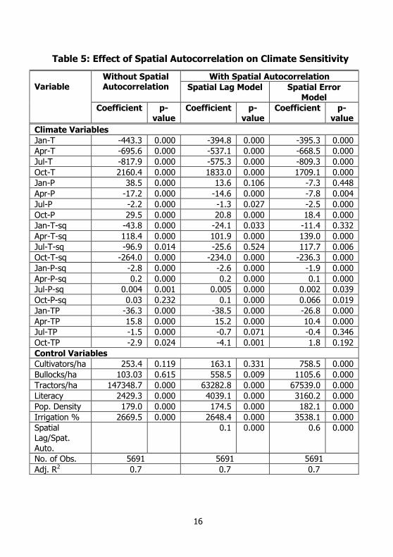
16

Table 5: Effect of Spatial Autocorrelation on Climate Sensitivity

Variable

Without Spatial Autocorrelation

With Spatial Autocorrelation

Spatial Lag Model Spatial Error Model

Coefficient p-value

Coefficient p-value

Coefficient p-value

Climate Variables

Jan-T -443.3 0.000 -394.8 0.000 -395.3 0.000

Apr-T -695.6 0.000 -537.1 0.000 -668.5 0.000

Jul-T -817.9 0.000 -575.3 0.000 -809.3 0.000

Oct-T 2160.4 0.000 1833.0 0.000 1709.1 0.000

Jan-P 38.5 0.000 13.6 0.106 -7.3 0.448

Apr-P -17.2 0.000 -14.6 0.000 -7.8 0.004

Jul-P -2.2 0.000 -1.3 0.027 -2.5 0.000

Oct-P 29.5 0.000 20.8 0.000 18.4 0.000

Jan-T-sq -43.8 0.000 -24.1 0.033 -11.4 0.332

Apr-T-sq 118.4 0.000 101.9 0.000 139.0 0.000

Jul-T-sq -96.9 0.014 -25.6 0.524 117.7 0.006

Oct-T-sq -264.0 0.000 -234.0 0.000 -236.3 0.000

Jan-P-sq -2.8 0.000 -2.6 0.000 -1.9 0.000

Apr-P-sq 0.2 0.000 0.2 0.000 0.1 0.000

Jul-P-sq 0.004 0.001 0.005 0.000 0.002 0.039

Oct-P-sq 0.03 0.232 0.1 0.000 0.066 0.019

Jan-TP -36.3 0.000 -38.5 0.000 -26.8 0.000

Apr-TP 15.8 0.000 15.2 0.000 10.4 0.000

Jul-TP -1.5 0.000 -0.7 0.071 -0.4 0.346

Oct-TP -2.9 0.024 -4.1 0.001 1.8 0.192

Control Variables

Cultivators/ha 253.4 0.119 163.1 0.331 758.5 0.000

Bullocks/ha 103.03 0.615 558.5 0.009 1105.6 0.000

Tractors/ha 147348.7 0.000 63282.8 0.000 67539.0 0.000

Literacy 2429.3 0.000 4039.1 0.000 3160.2 0.000

Pop. Density 179.0 0.000 174.5 0.000 182.1 0.000

Irrigation % 2669.5 0.000 2648.4 0.000 3538.1 0.000

Spatial Lag/Spat.

Auto.

0.1 0.000 0.6 0.000

No. of Obs. 5691 5691 5691

Adj. R2 0.7 0.7 0.7

17

All the estimates are based on fixed (year) effects specification in

the pooled data and observations are weighted by the total area under all

the crops considered in the analysis. Barring a few exceptions, the

climate coefficients in the models that accounts for spatial autocorrelation

(either through spatial lag or spatial error models) are uniformly lower

than that ignores the presence of spatial autocorrelation indicating the

true climate change impacts to be lower. This is confirmed by the climate

change impacts reported in table 6. The overall impacts estimated (for

same climate change scenario) using climate coefficients obtained from

model that accounts for spatial autocorrelation are significantly lower

than those obtained from model that ignores the spatial effects. Figures 2

compare the distribution of climate change impacts at the district level

between the model accounts for spatial autocorrelation and that does

not5.

Table 6: Climate Change Impacts – Without and With Spatial Autocorrelation

Scenario

Without Spatial Autocorrelation

With Spatial Autocorrelation

Spatial Lag Model Spatial Error Model

Impacts % of 1990 Net

Revenue

Impacts % of 1990 Net

Revenue

Impacts % of 1990 Net

Revenue

+2oC/7% -81.2 -9.17 14.2 1.6 -22.9 -2.6

India Specific CC Scenario

-195.1 -22.1 43.4 4.9 -2.1 -0.23

Note: Impacts are in billion rupees, 1999-2000 prices: Net revenue in

India in 1990 is Rs. 885 billion (1999-2000 prices).

5 Only spatial lag model results are reported for the purpose of comparison.

18

Figure 2. Distribution of Climate Change Impacts across Districts – Without and With Spatial

Autocorrelation

18

19

4. EVIDENCE ON INTER-FARMER COMMUNICATION

As observed in the previous section consideration of spatial effects has

contributed to positive spin-offs in terms of reduced climate change

impacts. For designing enabling policy responses, it is important to

explore factors contributing towards such spatial effects. Hypothesizing

that inter-farmer communication could among other factors be

responsible for spatial autocorrelation, an attempt has been made to

understand the scope and extent of information exchange between

farmers through focus group meetings held at six villages each in Tamil

Nadu and Andhra Pradesh1. The focus group meetings mainly explored

the perceptions of the villagers about the climate change and their views

on strategies helpful in ameliorating the climate change impacts. Among

other things, special attention is paid to the channels through which

information diffusion takes place.

The field level analysis showed that while most farmers are

familiar with the term climate change, their understanding is often

overlapping with other phenomenon. All climate/natural patterns are

perceived as climate change with little and/or no distinction between

future climate change and preset day climate concerns (that manifest in

the form of climate extremes like droughts, floods and cyclones, and

1 The focus group discussions are attempted only to gather preliminary insights

about the information exchange between several groups of farmers and by no

means these modest number of focus group discussions are claimed to reflect

the reality in the varied agricultural systems that are practiced in India. The

field studies are carried out during the months of March-April 2008 with the

help of local NGOs. In Tamil Nadu the villages covered include

Manampathy, Thevoor, Kumaramangalam, Echur, Arungunram, and

Thirunilai. In Andhra Pradesh Kothapatnam, Nidavanur, Kuchipudi,

Nilayeepalem, Chinagangam villages are covered for the focus group

discussions. Further, given the small number of discussions, no attempt has

been made to quantify the findings.

20

abnormal weather patterns like un-seasonal rainfall etc.). However, there

is a consensus in most discussions that anthropogenic activities leading

to excess pollution are often responsible for the abnormal weather.

Most farmers also consider climate/weather concerns to be more

threatening than other risks, such as price changes. The reasons cited for

such perceptions include, bigger scale of impact that climate/weather

risks may cause, and limited scope for adaptation. Such perceptions are

uniformly held by small, medium and large farmers.

Almost all focus group meetings indicated that there is dearth of

information. Farmers irrespective of size are in search of information –

which could include advice on input use, pest control, agronomic

practices, and soil and water conservation practices. Among the various

sources through which information diffusion takes place, most focus

group discussions ranked large farmers in the neighborhood as the

primary source. Not surprisingly, the agricultural extension services

offered by the government are not seen as appropriate source of

information, mainly due to the manner in which the extension services

provide information. While the information needs are different across

farmers based on their scale of operation and kind of crops cultivated,

the agricultural extension services often package the information in

uniform manner as though one size fits all. Similarly, the usual

information diffusion sources such as television and radio also appear to

be less effective in reaching out, partly because these sources are often

seen as entertainment sources rather than information channels.

Discussion in several focus group meetings revealed that farmers often

depend on fertilizer and pesticide dealers for information on new varieties

and new agricultural practices. While this source has appropriate self

regulated checks against provision of wrong information, it is important

to ensure that incorrect information does not reach the farmers even

inadvertently. Most importantly these sources provide information in a

case-by-case manner that suits most farmers.

21

New information does not often reach agricultural laborers. Given

the large size of this group and the important role it plays in determining

agricultural productivity, it is important to ensure that this group is also

targeted along with farmers in providing information on agricultural

practices. Similarly, the information diffusion must take place to reach

female farmers also alongside their male counterparts, which appeared to

be lacking presently based on the evidence from the focus group

discussions with the female farmers. There is two-tier structure for the

information flow with the male farmers receiving it first and the female

farmers learning through their male counterparts. Perhaps this is due to

larger social prejudices and needs immediate attention.

The field studies also revealed that new sources of information

diffusion should be explored and experimented. Given the fragmented

nature of Indian agricultural lands, large scale participation of corporate

sector in providing agricultural extension services could be difficult, and

hence other options must be explored. Among other things, the farmers

favored participation of agricultural cooperatives, NGOs, and dealers of

inputs and fertilizers in information diffusion. In this context, other

country experiences should also be carefully studied to identify the routes

through which the agricultural extension services could be provided to

the farmers. For instance, in Ecuador the agricultural extension workers

operate in tandem with the farmers through share cropping to ensure

proper information diffusion. On the other hand, Chile finances the costs

of private sector firms transferring the technology know-how and

information on new agricultural practices to small scale farmers.

22

5. CONCLUSIONS

The evidence presented in this paper suggests that (a) climate

change impacts are increasing over time indicating the increasing climate

sensitivity of Indian agriculture; and (b) accounting for spatial

autocorrelation is important due to the presence of significant spatial

clustering of the data; further, the climate change impacts are

significantly lower after incorporating spatial effects in the model

specification. The positive spatial effects could be due to the presence of

numerous communication channels between the „better-off‟ and „not-so-

better-off‟ farmers. Of course the information flow could also be in the

opposite direction. To exploit the presence of information flows between

the farmers, adaptation strategies through policy intervention can be

thought out to improve such channels. A crucial issue that should be

addressed in the context of adaptation is – how to adapt and adapt to

what.

The impact assessment literature mainly focused on what could

be termed as engineering/technological adaptation options. One measure

of the potential and cost of adaptation is to consider the historical record

of past speeds of adoption of new technologies. For example, Reilly and

Schimmelpfenng (1999) show the relative speed of adoption of various

adaptation measures. While the time taken for relatively soft adaptation

measures such as variety adoption and fertilizer adoption could be in the

range of 3 to 10 years, the hard options like development of irrigation

equipment and irrigation systems take much longer time. Jodha (1989)

also provides similar estimates based on evidence from post-independent

India. These adjustment times indicate that for effective implementation

of adaptation strategies appropriate planning must start well before the

manifestation of climate change. Also, soft options could be more cost

effective and hence should be explored first. Often the soft options

(which include enhancing the information flows mentioned above) may

23

provide dual advantage of gearing up for the future climate change as

well as providing benefits under the present-day conditions.

This leads the discussion to the next issue: adapt to what? This

has significant policy relevance in the ongoing discussion on

„mainstreaming‟ the climate policies. For vast majority of developing

countries (including India) climate change is a distant and invisible threat

whereas they are presently exposed to a range of stresses (including

climate related shocks such as cyclones, droughts and floods). If climate

change response strategies were to be embraced by these countries it is

imperative that such response strategies are aligned with development

agenda. Also, the local population should feel that the adaptation is

relevant and in their own interest. It is unrealistic to expect special policy

initiatives to deal with climate change adaptation by itself, especially

when so many of the suggested adaptation measures (such as drought

planning, coastal zone management, early warning etc.) are currently

being addressed in other policies and programs.

Underlying this is the implicit assumption that adaptation

strategies geared to cope with large climate anomalies that society faces

currently embrace a large proportion of the envelope of adjustments

expected under long-term climate change. In other words the climate

policies (at least in the local context) need not be something different

from the development policies. However, this need not be interpreted as

nullification of need for research on climate change specific adaptation

options. On the contrary the two should be seen as complimentary to

each other.

24

REFERENCES

Cline, W.R. (1996), “The Impact of Global Warming on Agriculture:

Comment” American Economic Review, 86(5): 1309-11.

Cline, W. (2007), Global Warming and Agriculture: Impact Estimates by

Country, Washington D.C., Peterson Institute.

Darwin, R. (1999), “The Impact of Global Warming on Agriculture: A

Ricardian Analysis: Comment”, American Economic Review,

89(4): 1049-52.

Deschenes, O. and M. Greenstone (2007), “The Economic Impacts of

Climate Change: Evidence from Agricultural Output and Random

Fluctuations in Weather”, American Economic Review, 97(1):

354-385.

Dinar, A., R. Mendelsohn, R. Evenson, J. Parikh, A. Sanghi, K. Kumar, J.

McKinsey, and S. Lonergan (1998), “Measuring the Imapct of

Climate Change on Indian Agriculture”, Technical Paper 402,

World Bank, Washington, D.C.

Jodha, N.S. (1989), “Potential Strategies for Adapting to Greenhouse

Warming: Perspectives from the Developing World”, In

Rosenberg, N.J., W.E. Easterling, P.R. Crosson, and J.

Darmstadter (eds.). Greenhouse Warming: Abatement and

Adaptation. Washington D.C.: Resources for the Future.

Kumar, K.S. Kavi, and J. Parikh (2001a), “Socio-economic Impacts of

Climate Change on Indian Agriculture”, International Review of

Environmental Strategies, 2(2): 277-293.

Kumar, K.S. Kavi, and J. Parikh (2001b), “Indian Agriculture and Climate

Sensitivity”, Global Environmental Change, 11(2): 147-154.

Mall, R.K., R. Singh, A. Gupta, G. Srinivasan, and L.S. Rathore (2006),

“Impact of Climate Change on Indian Agriculture: A Review”,

Climatic Change, 78: 445-478.

25

Mendelsohn, R., A. Dinar, and A. Sanghi (2001), “The Effect of

Development on the Climate Sensitivity of Agriculture”,

Environment and Development Economics, 6(1): 85-101.

Mendelsohn, R., W. Nordhaus, and D. Shaw (1994), “The Impact of

Global Warming on Agriculture: A Ricardian Analysis”, American

Economic Review, 84(4): 753-71.

Polsky, C. (2004), “Putting space and time in Ricardian climate change

impact studies: Agriculture in the US Great Plains, 1969-1992”,

Annals of the Association of American Geographers, 94(3): 549-

564.

Quiggin, J. and J. K. Horowitz (1999), “The Impact of Global Warming on

Agriculture: A Ricardian Analysis: Comment”, American Economic

Review, 89(4): 1044-45.

Reilly, J.M. and D. Schimmelpfennig (1999), “Agricultural Impact

Assessment, Vulnerability, and the Scope for Adaptation”,

Climatic Change, 43: 745-788.

Sanghi, A. and R. Mendelsohn (2008), “The Impacts of Global Warming

on Farmers in Brazil and India”, Global Environmental Change,

18: 655-665.

Schlenker, W., W.M. Hanemann and A.C. Fisher (2005), “Will US

agriculture really benefit from global warming? Accounting for

irrigation in the Hedonic approach”, American Economic Review,

95(1): 395-406.

Schlenker, W. and M. Roberts (2008), Estimating the Impact of Climate

Change on Crop Yields: The Importance of Non-linear

Temperature Effects, Working Paper 13799. Cambridge: National

Bureau of Economic Research.

26

Solomon, S., D. Qin, M. Manning, Z. Chen, M. Marquis, K.B. Averyt, M.

Tignor and H.L. Miller, eds. (2007), Climate Change 2007: The

Physical Science Basis, Contribution of Working Group I to the

Fourth Assessment Report of the Intergovernmental Panel on

Climate Change, Cambridge: Cambridge University Press.

Stern, N. (2006), The Economics of Climate Change: The Stern Review,

Cambridge: Cambridge University Press.

World Bank (2008), Climate Change Impacts in Drought and Flood

Affected Areas: Case Studies in India, Report No. 43946-IN; New

Delhi: India Country Management Unit.

MSE Monographs

* Monograph 1/2006 A Tract on Reform of Federal Fiscal Relations in India Raja J. Chelliah

* Monograph 2/2006 Employment and Growth C. Rangarajan

* Monograph 3/2006

The Importance of Being Earnest about Fiscal Responsibility C. Rangarajan and Duvvuri Subbarao

* Monograph 4/2007 The Reserve Bank and The State Governments: Partners in Progress Y.V.Reddy

* Monograph 5/2008

India’s Dilemmas: The Political Economy of Policy-Making in a Globalized World Kaushik Basu

MSE Working Papers Recent Issues

* Working papers are downloadable from MSE website http://www.mse.ac.in $ Restricted circulation

$ Working Paper 34/2008 Customer Relationship Management (Crm) to Avoid Cannibalizat ion: Analysis Through Spend Intensity Model Saumitra N Bhaduri, Avanti George and David J Fogarty

* Working Paper 35/2008 Innovation in India and China: Challenges and Prospects in Pharmaceuticals and Biotechnology

Jayan Jose Thomas

* Working Paper 36/2008 An Analysis of Life Insurance Demand Determinants for Selected Asian Economies and India Subir Sen

* Working Paper 37/2008 The Impact of R&D and Foreign Direct Investment on Firm Growth in Emerging-Developing Countries: Evidence rom Indian Manufacturing Industries Adamos Adamou and Subash S

* Working Paper 38/2008 Stock Returns-Inflation Relation in India

K.R. Shanmugam and Biswa Swarup Misra

* Working Paper 39/2009

Designing Fiscal Transfers: A Normative Approach K.R. Shanmugam and D.K. Srivastava

* Working Paper 40/2009 Determining General and Specific Purpose Transfers: An Integrated Approach Richa Saraf and D.K. Srivastava

* Working Paper 41/2009 Socio-Economic Characteristics of the Tal l and Not So Tall Women of India Brinda Viswanathan and Viney Sharma

* Working Paper 42/2009 Inter-State Imbalances in Essential Services: Some Perspectives C. Bhujanga Rao and D.K. Srivastava

* Working Paper 44/2009 Finance Commission and The Southern States: Overview of Issues D.K.Srivastava (forthcoming)