climate in a box user’s guide to models - nasa · climate in a box user’s guide to models...

Climate In a Box Userrsquos Guideto Models

Robert Burns Carlos Cruz Shawn Freeman

Philip Hayes Ramon Linan Raj Pandian

Rahman Syed Bruce VanAartsen and Gary

Wojcik

Software Integration andVisualization Office

NASA Goddard Space Flight CenterGreenbelt MD 20771

February 3 2011

Contents

1 System Overview 5

11 Toolkit platform hardware 5

12 Toolkit platform software 6

2 NASA Modeling Guru Knowledge Base and Forums 8

3 Torque Scheduler 11

4 NASA Workflow Tool 13

41 Tools and Data 13

42 General Operations 13

43 User Setup 14

44 Workflow Tool Installation 15

5 GEOS-5 AGCM 16

51 Configuring and building 18

511 MERRA vs Fortuna Tags 18

512 Baselibs 19

52 Installing the Fortuna Tag 20

53 Input dataBoundary conditions 22

54 Setting Up An Experiment 22

541 RC Files 26

55 Output and Plots 28

CONTENTS 3

56 Case Study 28

6 NASA-GISS modelE 30

601 System requirements 30

61 Configuration and Building 31

611 Getting the code 31

612 configuring modelE 32

613 Model installation 34


63 Executing an experiment 36

64 Visualization 37

641 Post-processed output 38

65 Stand-alone Package 40

651 Case Study 42

7 WRF 43

71 Introduction 43

72 Obtaining the Code 44

73 Configuring and building WRF model 44

731 Create a working directory 44

732 Initial Settings 45

74 Compiling WRF 46

75 Compiling WPS 47

76 Steps to Run Geogrid 50

77 Steps to Run Ungrib 50

78 Steps to Run Metgrid 51

79 Steps to Run WRF 52

710 Case Study Description 53

711 Run Case Study 54

8 GFDL MOM4 55

CONTENTS 4


811 Solo Models 56

812 Coupled Models 57


82 Examining the output 57

83 MOM4 Test Cases 58

9 FAQ and tips 61

91 Compiler settings 61

92 Links to documentation 61

Chapter 1

System Overview

Thank you for your participation in the Climate in a Box (CIB) projectAt NASArsquos Software Integration and Visualization Office (SIVO) we hopeto create a system that will make climate and weather research far moreaccessible to the broader community Although the project currently servesusers with a basic software toolkit wersquore moving forward with improving theuser experience of data and code sharing

With the Climate Toolkit our focus has been more on software thanhardware Although wersquore moving toward our goal for any user to deploy theCIB Toolkit on any cluster with minimum hassle for now wersquore deliveringthe software pre-installed onto new rdquodesktop supercomputersrdquo from SGI andCray

This Userrsquos Guide will provide CIB participants with a detailed set ofinstructions on how to administer a desktop supercomputer configured bySIVO how to execute the models that have been installed and how to con-figure new experiments moving forward

11 Toolkit platform hardware

The desktop supercomputers available so far have had a configuration similarto this details may not be exact for all systems

bull 1 chassis with 8-10 rdquobladesrdquo or rdquonodesrdquo


bull Node configuration

ndash 2 quad-core Intel Xeon cpus (8 cores total)

ndash 24gb RAM

ndash 300gb hard drive

bull Internal InfiniBand network for high-speed MPI communication

bull Internal Gigabit Ethernet network for administration

bull External Gigabit Ethernet interface on headnode for Internet connec-tivity

12 Toolkit platform software

The strategy for the Climate Toolkit is to emulate the major software compo-nents found on the NASA Center for Climate Simulation (NCCS) rdquoDiscoverrdquosupercomputing cluster Developers benefit from having an environment sim-ilar across platforms so any porting effort is made easier

For the first version of the Climate Toolkit SIVO has selected CentOS55 a community-supported version of RedHat Enterprise Linux With theOSCAR cluster toolkit and Torque scheduling system this provides a solidplatform for high performance computing (HPC) development More infor-mation about these software packages can be found at these links

httpwwwcentosorghttpsvnoscaropenclustergrouporgtracoscar

The Climate Toolkit will be based on versions 91 101 and 111 of IntelrsquosCompiler Suite (for CC++Fortran) To reduce complexity we have chosento support only the mvapich2 MPI library so the models and software becomemore manageable

The computational environment is managed using the module package(see httpmodulessourceforgenet) The module package allows for thedynamic modification of a userrsquos computational environment using ldquomodulecommandsldquo thus allowing to chooseswitch among various combinations of


compilers and MPI libraries To get started type ldquomodule helpldquo For ex-ample to view a list of installed compilers and MPI libraries type ldquomoduleavailldquo

We have also installed the NASA Workflow Server to make model setupand execution easy for new users Users are encouraged to develop their ownworkflows to make management and preservation of different experimentsmuch simpler

Chapter 2

NASA Modeling GuruKnowledge Base and Forums

NASAs Modeling Guru website is a user-friendly tool that allows those in-volved in Earth science modeling and research to find and share relevantinformation The system hosts a growing repository for expertise in run-ning Earth science models and using associated high-end computing (HEC)systems It is open to the public allowing collaboration with scientists pro-fessors and students from external research institutions

This Web 20 site offers

Topic-based communities for various scientific models software toolsand computing systems (ie Climate in a Box community)

Each community has its own discussion forums wiki-type documentsand possibly blogs

E-mail notifications or RSS feeds for desired communities or blogs

Homepage customization with drag-and-drop widgets

Publicly available at httpsmodelinggurunasagov

If you register for an account youll be able to post questions receive emailnotifications and customize you homepage View registration instructions byclicking Request an Account at the top of the pageNCCS account-holders

9

Figure 21 Climate in a Box Community in the NASA Modeling Guru WebSite

(for Discover Dirac etc) are preregistered ndash just login with your currentusername and password

For CIB users most relevant resources would be the found in the Cli-mate in a Box community which can be found by clicking its link underthe Communities menu on the homepage or by using this direct URLhttpsmodelinggurunasagovcommunitysystemsclimateinabox

Figure 21 shows a portion of the Overview page for the Climate in a BoxCommunity

Note that the tabs at the top let you select a specific content type toview Documents include information like model run procedures or bench-mark results while Discussions are your forum for posting questions If youdlike to be notified about all new posts to this community click Receive emailnotifications on the right (must be logged in to see this option)

10

If you cant find information you need on the site click Start a Discussionto post your question Moderators will monitor this area and will normallyrespond the same day We also expect to have a live-chat support featurewhich should be available most days during business hours

Chapter 3

Torque Scheduler

The Torque Scheduler is software that allows for several users on a clusterto share the nodes efficiently It is similar in operation to the PBS Prosoftware used on the NCCS Discover cluster Users recognize it as the rdquoqsubrdquocommand

For extensive documentation please visit the Torque website

httpwwwclusterresourcescomproductstorque-resource-managerphp

Most end users will find all they need here

httpwwwclusterresourcescomproductstorquedocs21jobsubmissionshtml

Users can create scripts that launch MPI tasks and submit them in thebackground for execution Queues are available so that users can reserve thesystem for their experiment and release it others when their job finishes Thefollowing directives should be placed at the top of a user script

PBS -S binbash

PBS -N somejobname

PBS -l nodes=2ppn=8

PBS -l walltime=003000

Once the user script has been created that loads the right applicationmodules cd to the correct directory then a user can submit this job to thequeue by typing rdquoqsub run scriptbashrdquo

12

Submitting a script to the background is one way of using the computa-tional resources on these clusters Another useful way is called an rdquointeractivePBS sessionrdquo which can help with debugging problems This method allowsa user to have their terminal rdquolandrdquo on a compute node where he can launchMPI applications directly Herersquos a sample session

[someuserheadnode run]$ hostname

headnodecx1

[someuserheadnode run]$ qsub -I -l nodes=2ppn=8walltime=003000

qsub waiting for job 1505headnodecx1 to start

qsub job 1505headnodecx1 ready

[someusernode-7 ~] hostname

node-7cx1

[someusenode-7 ~]$ mpirun_rsh -np 16 somemodelx

With an interactive session a script is not provided to the qsub commandInstead a user must use the rdquo-Irdquo flag to indicate that it is an interactivesession as well as the PBS parameters to indicate how many resources hewould like to use

Users must remember to type rdquoexitrdquo to leave an interactive session whentheyrsquore finished otherwise resources might sit idly while other users cannotaccess them

Chapter 4

NASA Workflow Tool

41 Tools and Data

The workflow tool is set up on the CIB system under the following paths

cibworkflow tool - Contains the initial workflow configurationsworkflow datasets experiment runs and other workflow-specific infor-mation

ciboutputdataltusernamegtworkflow - Typically contains thelarge outputs generated by workflows Note that Generic User modein NED places outputs under the ciboutputdataworkflowworkflowfolder

optandciblibraries - Contains various tools and applications re-quired to run the workflow tool or individiual workflows

optNEDandciblibrariesworkflow - Contains the NASA Ex-periment Designer client server and workflow editing software

42 General Operations

The workflow tool requires three processes to be launched during systemreset These processes should generally be run by the dedicated workflowaccount

43 User Setup 14

To start the NED server

nohup optNEDserver_deploymentrunNedServersh gt ~

nedserverNohuplog

To start the eXist database which is used to track experiments

nohup opteXistbinstartupsh gt ~existNohuplog

To create a tunnel to the GEOS5 revision control server

NOTE Currently the tunnel to cvsacl is restricted and requires dual-factor authentication Because of this a tunnel must be set up using anNCCS passcode Due to NCCS policy this tunnel will currently only stayactive for 7 days This is only required for checkouts of GEOS5 with theworkflow)

nohup ssh usernamecvsacl gt nohup_cvsacllog

After this you will be prompted for your passcode and your passwordOnce you have entered the password you can press CTRL Z to backgroundthe tunnel To ensure that the tunnel has connected properly you can checkthe log file output

43 User Setup

At a bare minimum all users that will be running workflows must belongto the user group that will correspond to running workflows Currently thisgroup is the CIB group Admins of the box may add additional groups forcontrolling access to different workflow directories

Assuming that a global profile has been established following the instal-lation instructions no additional user setup is required for running generalworkflows

If a user or users wish to run workflows as themselves instead of usingthe generic workflow account then the user would be required to add thepublic SSH key of the workflow account running the server into the usersSSH authorized keys file


44 Workflow Tool Installation

Please refer to the NASA Workflow Tool Administrator Guide section ondeploying the NED server for information about setting up and installing theworkflow tool and its dependencies

Chapter 5

GEOS-5 AGCM

The Goddard Earth Observing System (version 5) suite and its AtmosphericGeneral Circulation Model (AGCM) are being developed at the Global Mod-eling and Assimilation Office (GMAO) to support NASArsquos earth science re-search in data analysis observing system modeling and design climate andweather prediction and basic research

The AGCM is a weather-and-climate capable model being used for atmo-spheric analyses weather forecasts uncoupled and coupled climate simula-tions and predictions and for coupled chemistry-climate simulations Thereare model configurations with resolutions ranging from 2o to 14o and with72 layers up to 001 hPa resolving both the troposphere and the stratosphere

The AGCM structure consists of a hierarchy of ESMF gridded compo-nents ([1]) constructed and connected using MAPL MAPL is a softwarelayer that establishes usage standards and software tools for building ESMFcompliant components The modelrsquos architecture is illustrated in figure 51Most of the calculations are done by components at the leafs of this treeThe composite components above the leafs serve as connectors performingspecialized connections between the children and producing combined out-puts

Parallelization is primarily implemented through MPI although somekey parts of the code such as the model dynamics also have Open-MPcapability The model runs on a 2-D decomposition transposing internallybetween horizontal and vertical layouts Some of the physics such as thesolar radiation which at any given time is active over only half the globe

17

Figure 51 The GEOS-5 AGCM structure


is load balanced The code scales well across compute nodes and scalabilityincreases linearly with problem size

For additional information see the GMAO GEOS5 web site

51 Configuring and building

The GEOS-5 AGCM can be potentially built on a variety of platforms in-cluding SGI IBM Darwin and Linux systems However most of our testingand portability tools are limited to a handful of Linux systems In the follow-ing sections we provide information on setting up and running one versionof the AGCM Fortuna 21 Other versions of GEOS-5 may differ in detailsthat while minor will require different steps for building and running socaveat utilitor

The following description assumes that you know your way around Unixhave successfully logged into your NCCS account (presumably on the DIS-COVER cluster) and have an account on progress with the proper ssh prepa-ration (see the progress repository quick start) However the same commandscan be used in the CIB system unless otherwise noted

The commands below assume that your shell is csh This is for conve-nience since the scripts to build and run GEOS-5 tend to be written in thesame shell If you prefer or use a different shell it is easiest just to open acsh process to build the model and your experiment

511 MERRA vs Fortuna Tags

MERRA refers to the NASA reanalysis data set that uses a major new versionof the GEOS-5 Data Assimilation System ([3]) In the context of Climate Ina Box (CIB) MERRA is that and additionally it refers to the particularAGCM code base (tag) used in the generation of the MERRA data set1

The newest set of code releases are named Fortuna and the latest stabletag is Fortuna 21 (henceforth referred to as simply Fortuna)

The CIB toolkit is loaded with both the MERRA and Fortuna tags Thenext section describes the minimum steps required to build and run GEOS-5

1The tag GEOSagcm-Eros 7 25 was part of the Eros family of code releases


Fortuna 21 on a Linux platform You should successfully complete the stepsin these instructions before doing anything more complicated

Note that as packaged the MERRA tag must be built using a differentcompiler version As we shall see Fortuna uses Intel 111 whereas MERRArequires Intel 91 (and will work with Intel 101)

512 Baselibs

Baselibs are a set of support libraries (ESMF HDF netCDF etc) that needto be installed before attempting to build the GEOS-5 AGCM applicationNote that the CIB toolkit will contain preinstalled Baselibs for both theMERRA and Fortuna tags In this section we provide a brief description ofBaselibs installation

Note that the following compilers and utilities are required for compilingand building the Baselibs

- Fortran90 (or later) compiler

- C compiler

- MVAPICH2 openMPI or intel MPI compatible with the above com-pilers

- GNU make

- Perl - to run some scripts

- LATEX - to produce documentation

and the same should be used to build the Fortuna tag

Building the Baselibs from scratch requires an account on NASA-GSFCNCCS systems to access the progress repository as well as permission to readthe baselibs repository

When you have permission to checkout the Baselibs software from theprogress repository login to your target system and issue these commands

setenv CVS_RSH ssh

cvs -d extUSERNAMEprogressnccsnasagovcvsrootbaselibs

checkout -r SOMETAG Baselibs


Please replace USERNAME with your LDAP userid Please replaceSOMETAG with a valid Baselibs tag If you are using GEOS consider tagrdquoGMAO-Baselibs-3 2 0rdquo which is compatible with the Fortuna 21 tag Alsoplease note that the module name is rdquoBaselibsrdquo case sensitive

Other available tags

GMAO-Baselibs-3_1_4 (use with Fortuna 1x tags)

GMAO-Baselibs-2_1_1 (use with MERRA tag must be build with Intel 91 compiler)

For each system the environment must be setup so the build process willuse the desired compilers The Baselibs are generally portable but tweaksmay be needed and their discussion is beyond the scope of this manualTherefore it is recommended that the user refer to NASA Modeling Guruweb site

When issuing the make commands found in the INSTALL documentitrsquos best to route all output into a log file for debugging purposes Use thefollowing conventions to capture all information and run the installation inthe background

To install

make install gtamp installlog amp

You can also issue a rdquotail -f installlogrdquo to watch the process run to com-pletion if yoursquod like

When the process has completed search installlog for the keyword rdquoEr-rorrdquo Ignore any rdquoErrorrdquo string thatrsquos found in a filename or as part of acompiler warning If there are legitimate errors please review your environ-ment setup and build command prior to contacting support

After installation is complete the environment variable BASEDIR speci-fying the path of the Baselibs must be set

52 Installing the Fortuna Tag

Set the following environment variable

setenv CVSROOT extUSERIDprogressnccsnasagovcvsrootesma


where USERID is of course your progress username which should bethe same as your NASA and NCCS username Then issue the command

cvs co -r Fortuna-2_1 Fortuna

This should check out the Fortuna version of the model from progress andcreate a directory called GEOSagcm If you cd into GEOSagcmsrc thereis a script g5 modules that can be used to setup the proper computationalenvironment on NCCS systems otherwise it will likely not be portable Ifyou are working on NCCS systems

source g5_modules

Else on the CIB system use the script provided under ciblibrariesarchives

cp ciblibrariesarchivesset_modeltyour shellgt ~

To use execute the script and it will provide usage instructions When donetype

module list

and you should see

Currently Loaded Modulefiles

1) compintel-111

2) mpimvapich2-15intel-111

And the following environment variables must be set

setenv BASEDIR ltPATHS WHERE BASELIBS ARE INSTALLEDgt

setenv LD_LIBRARY_PATH $LIBRARY_PATH$BASEDIR$archlib

The environment variable BASEDIR was described in the previous sec-tion The environment variable LD LIBRARY PATH is a colon-separated setof directories where libraries should be searched for first before the standardset of directories On the MAC this variable is called DYLD LIBRARY PATHOn the CIB system the set mode script will take care of this

If this all worked then type


gmake install gt amp makefilelog amp

This will build the model and redirect the gmake output to the make-filelog file You can check the gmake progress by typing rdquotail -f makefilelogrdquoThe installation will take about 45 minutes If this works it should createa directory under GEOSagcm called Linuxbin In here you should find theexecutable GEOSgcmx

53 Input dataBoundary conditions

NOTE To obtain data from outside the NCCS firewall users must log into the data migration facility (DMF) The NCCS is currently running DMFon an SGI Origin 3000 called palm and the host name for the public-facingsystem is diracgsfcnasagov

What input data (ICs BCs resource files) do we need to run a GEOS-5AGCM experiment Generally model input - including restarts and resourcefiles - is associated with a particular CVS rdquotagrdquo like MERRA and FortunaThe CIB toolkit provides data sets to be used with the MERRA and Fortunatags at 2o resolution Currently there is no easy way to gather up all thenecessary data to run a particular experiment at a specific resolution If youneed a specific data set please contact SIVO

54 Setting Up An Experiment

First of all to run jobs on the cluster you will need to set up passwordlessssh (which operates within the cluster) On the CIB system there is nothingto do On the NCCS cluster run the following from your home directory

cd ssh

ssh-keygen -t dsa

cat id_dsapub gtgt authorized_keys

Similarly if working on the NCCS cluster transferring the daily outputfiles (in monthly tarballs) requires passwordless authentication from DIS-COVER to PALM While in simssh on DISCOVER run


ssh-keygen -t dsa

Then log into PALM and cut and paste the contents of the id rsapuband id dsapub files on DISCOVER into the simsshauthorized keys file onPALM Problems with ssh should be referred to NCCS support

To set the model up to run we need to create an experiment directory(scratch) that will contain GEOSgcmx restarts BCs and resource files Onthe CIB system the system can be setup using the experiment setup toolcontained in cibmodelsarchive These are the steps to follow

cp cibmodelsarchiveAGCMsetuptgz ciboutputdataltuseridgt

tar xfz AGCMsetuptgz

cd AGCMsetup

EDIT optionsrc file

RUN setupg5gcm

AGCMsetup helps setup MERRA or Fortuna run (2o resolution only)but we still need to create a run script A sample one fortuna runj can beobtained from cibmodelsarchives with only a minor edit necessary

On NCCS systems the GEOSagcmsrcApplicationsGEOSgcm App di-rectory contains the script gcm setup than can also be adapted to the CIBsystem To run

gcm_setup

The gcm setup script asks you a few questions such as an experimentname (with no spaces called EXPID) and description (spaces ok) It willalso ask you for the model resolution expecting one of the available lat-londomain sizes the dimensions separated by a space Here are some detailsregarding the required input

- The Experiment ID should be an easily identifiable name representingeach individual experiment you create One possibility is your initialsfollowed by a 3-digit number abc001

- The Experiment Description should be a concise statement describingthe relevant nature of your experiment


- Model Resolution Options

72 46 (~ 4 -deg)

144 91 (~ 2 -deg)

288 181 (~ 1 -deg)

576 361 (~12-deg)

1152 721 (~14-deg)

- The AERO PROVIDER describes the Chemistry Component to beused for Radiatively Active Aerosols PCHEM is the default used formost AMIP-style Climate Runs

- The HOME directory will contain your run scripts and primary resource(rc) files

- The EXP directory will contain your restarts and model outputThe HOME and EXP directories can be the same egdiscovernobackup$LOGNAMEabc001

- Your GROUP ID is your charge code used for NCCS accounting (notrequired on CIB)

For your first time out you will probably want to enter 144 91 (corre-sponding to sim2 degree resolution) Towards the end it will ask you for agroup ID Enter whatever is appropriate as necessary The rest of the ques-tions provide defaults which will be suitable for now so just press enter forthese Note that gcm setup will not work outside of NCCS systems

The script produces an experiment directory (EXPDIR) in your space(on DISCOVER) as discovernobackupUSERIDEXPID which containsamong other things the sub-directories

- post (containing the post-processing job script)

- archive (containing an incomplete archiving job script)

- plot (containing an incomplete plotting job script)

The post-processing script will complete (ie add necessary commandsto) the archiving and plotting scripts as it runs The setup script that you ran


also creates an experiment home directory (HOMEDIR) as simUSERIDgeos5EXPIDcontaining the run scripts and GEOS resource (rc) files

The run scripts need some more environment variables here are the min-imum contents of a cshrc

umask 022

unlimit

limit stacksize unlimited

set arch = lsquounamelsquo

The umask 022 is not strictly necessary but it will make the various filesreadable to others which will facilitate data sharing and user support Yourhome directory simUSERID is also inaccessible to others by default runningchmod 755 sim is helpful

Copy the restart (initial condition) files and associated cap restart intoEXPDIR Keep the rdquooriginalsrdquo handy since if the job stumbles early in therun it might stop after having renamed them The model expects restart file-names to end in rdquorstrdquo but produces them with the date and time appended soyou may have to rename them The cap restart file is simply one line of textwith the date of the restart files in the format YYYYMMDDltspacegtHHMMSSThe boundary conditionsforcings are provided by symbolic links created bythe run script If you need an arbitrary set of restarts please contact SIVO

The script you submit gcm runj is in HOMEDIR It should be readyto go as is The parameter END DATE in CAPrc (previously in gcm runj)can be set to the date you want the run to stop You may edit the rc filesdirectly instead of template (tmpl) An alternative way to stop the runis by commenting out the line if ( $capdate lt $enddate ) qsub $HOME-DIRgcm runj at the end of the script which will prevent the script frombeing resubmitted or rename the script file You may eventually want totune parameters in the CAPrc file JOB SGMT (the number of days per seg-ment the interval between saving restarts) and NUM SGMT (the number ofsegments attempted in a job) to maximize your run time

Submit the job with qsub gcm runj On DISCOVER you can keep trackof it with qstat or qstat mdash grep USERID or stdout with tail -f DIS-COVERpbs spoolJOBIDOU JOBID being returned by qsub and dis-played with qstat Jobs can be killed with qdel JOBID The standard out


and standard error will be delivered as files to the working directory at thetime you submitted the job

541 RC Files

You need to edit a couple of files in HOMEDIR to get the experiment to runthe way you want

AGCMrc

This file controls the model run characteristics For example a particularAGCMrc file has the following lines characteristic (to run GOCART withclimatological aerosol forcing)

GOCART_INTERNAL_RESTART_FILE gocart_internal_rst

GOCART_INTERNAL_RESTART_TYPE binary

GOCART_INTERNAL_CHECKPOINT_FILE gocart_internal_checkpoint

GOCART_INTERNAL_CHECKPOINT_TYPE binary

AEROCLIM ExtDataAeroComL72aero_clmgfedv2aeroetay4m2clmnc

AEROCLIMDEL ExtDataAeroComL72aero_clmgfedv2del_aeroetay4m2clmnc

AEROCLIMYEAR 2002

DIURNAL_BIOMASS_BURNING no

RATS_PROVIDER PCHEM options PCHEM GMICHEM STRATCHEM

(Radiatively active tracers)

AERO_PROVIDER PCHEM options PCHEM GOCART

(Radiatively active aerosols)

To run with interactive aerosol forcing modify the appropriate lines aboveto look like



AEROCLIMYEAR 2002

AERO_PROVIDER GOCART options PCHEM GOCART



HISTORYrc

This file controls the output streams from the model These are know ascollections

COLLECTIONS rsquogeosgcm_progrsquo

rsquogeosgcm_surfrsquo

rsquogeosgcm_moistrsquo

rsquogeosgcm_turbrsquo

rsquogeosgcm_gwdrsquo

rsquogeosgcm_tendrsquo

rsquogeosgcm_budrsquo

rsquotavg2d_aer_xrsquo

rsquoinst3d_aer_vrsquo

Additional information about the HISTORYrc file can be found in thislink

CAPrc

Among other things this file controls the timing of the model run Forexample you specify the END DATE the number of days to run per segment(JOB SGMT) and the number of segments (NUM SGMT) If you modifynothing else the model would run until it reached END DATE or had runfor NUM SGMT segments

cap restart

This file doesnrsquot exist here by default so create it with your favorite edi-tor As explained earlier cap restart will have the model start date (ignoreBEG DATE in CAPrc if this file exists it supersedes that) It should justspecify YYYYMMDD HHMMSS start time of model run For example

19991231 210000

Additional information can be found here and at the GEOS5 wiki site


55 Output and Plots

During a normal run the gcm runj script will run the model for the seg-ment length (current default is 8 days) The model creates output files(with an nc4 extension) also called collections (of output variables) in EX-PDIRscratch directory After each segment the script moves the output tothe EXPDIRholding and spawns a post-processing batch job which parti-tions and moves the output files within the holding directory to their owndistinct collection directory which is again partitioned into the appropri-ate year and month The post processing script then checks to see if a fullmonth of data is present If not the post-processing job ends If there is a fullmonth the script will then run the time-averaging executable to produce amonthly mean file in EXPDIRgeos gcm The post-processing script thenspawns a new batch job which will archive (on DISCOVER) the data ontothe mass-storage drives (archiveuUSERIDGEOS50EXPID)

If a monthly average file was made the post-processing script will alsocheck to see if it should spawn a plot job Currently our criteria for plottingare

1) if the month created was February or August AND

2) there are at least 3 monthly average files

then a plotting job for the seasons DJF or JJA will be issued

The plots are created as gifs in EXPDIRplots The post-processingscript can be found in

GEOSagcmsrcGMAO_SharedGEOS_Utilpostgcmpostscript

The nc4 output files can be opened and plotted with gradsnc4 but usesdfopen instead of open See the Grads web site for a tutorial

The contents of the output files (including which variables get saved) maybe configured in the HOMEDIRHISTORYtmpl ndash a good description of thisfile may be found on Modeling Guru

56 Case Study

The setup provided in AGCMsetuptgz is intended to produce an experimen-tal setting with the following characteristics

56 Case Study 29

- Resolution 144x91x72 levels

- 5-day simulation with starting datetime 19920110 210000

- Comprehensive prognostic and diagnostic output over the simulationperiod

- 16cpu run (2 nodes)

The case study can be used as a benchmarking suite to port the modelamong platforms and to examine model reproducibility (see for example thisdocument) and to some extent performance (see this document)

Chapter 6

NASA-GISS ModelE

The most current version of the NASA-GISS series of coupled atmosphere-ocean models is called ModelE The ModelE source code can be down- loadedfrom the GISS web site Model documentation including the ModelE speci-fication and results from three standard configurations is given in [4]

The CIB system comes with a pre-installed version of modelE (8102010snapshot) In this chapter we describe the steps required to build install andrun modelE on the CIB system The CIB system also contains a stand-alonepackage to help expedite the experiment setup and is described in section65

601 System requirements

System requirements are the following

- Fortran 90 (or later) compiler

- C compiler


- GNU make (version 379 or higher)

- Perl (version 5005 or higher)


ModelE has been tested with the SGI IBM and COMPAQDEC com-pilers on their respective workstations For Linux Macs or PCs the choiceof compiler is wider

Parallelization is primarily implemented through MPI but some parts ofthe code also have Open-MP capability

Many GCM subroutines declare temporary arrays which in FORTRANreside in a part of the computerrsquos memory known in computer parlance as therdquostackrdquo It is essential that a userrsquos stack size be large enough to accommo-date these arrays a minimum value of 8192 kilobytes is recommended withstack requirements increasing with model resolution Default stack sizes varyamong different computing environments but can be easily adjusted Un-fortunately this parameter must be explicitly set by the user rather than bythe GCM setup scripts Stack size is set by commands native to a userrsquos$SHELL for example a bash user would type rdquoulimit -s 32768rdquo to get astack size of 32768 kb Mysterious crashes in the radiation are quite oftenrelated to a too small stack

61 Configuration and Building

611 Getting the code

To buildrun the latest modelE code base you will need to check it out fromthe GISS repository That requires an account on the GISS server Pleasecontact contact Gavin Schmidt at GISS

After you have gained access to the server you can checkout the code asfollows

export CVSROOT=simplexgissnasagovgisscvsroot

export CVS_RSH=ssh

cvs co modelE

This will get you the latest code snapshot The distribution of modelE hasa top directory named modelE which contains the following sub-directories

aux config decks E2000 init_cond model README tests

cmor CVS doc exec Makefile prtdag templates


The CVS directory is for version control purposes and may also be foundin the sub-directories

612 configuring modelE

The very first step in the modelE setup is to create of a file called model-Erc This file keeps some system-wide information (such as your directorystructure) which is common to all modelE runs you do on current machineTo create this file go to the directory modelEdecks and execute

gmake config

Note file name requires a rdquordquo dot This file must be placed on your homedirectory The file contains global options for modelE some of which mustbe modified The following is a sample modelErc file

This file contains global options for modelE

Directory structure

DECKS_REPOSITORY - a directory for permanent storage of run info

All rundecks that you create will be copied to this directory

DECKS_REPOSITORY=ciboutputdataccruz2modelEscratchdecks

CMRUNDIR - directory to which all run directories will be linked

This directory will be searched by most scripts for locations of

specific runs

CMRUNDIR=ciboutputdataccruz2modelEscratchcmrun

EXECDIR - path to directory with modelE scripts and with some

executables This directory should contain the scripts from modelEexec

EXECDIR=ciboutputdataccruz2modelEscratchexec

SAVEDISK - a directory where all run directories (which will contain

all output files such as rsf acc etc) will be created This should

be big enough to accomodate all model output

SAVEDISK=ciboutputdataccruz2modelEscratchout


GCMSEARCHPATH - directory to search for gcm input files

All necessary input files should be copied or linked to this directory

GCMSEARCHPATH=cibinputdatamodeleinput

NETCDFHOME - path to location of netcdf library Leave blank if netcdf

is not installed on this computer

NETCDFHOME=ciblibrariesnetcdf

Customizable setings for Makefile

OUTPUT_TO_FILES - if set to YES all errors and warnings will be sent

to files with the names ltsource_namegtERR

OUTPUT_TO_FILES=YES

VERBOSE_OUTPUT - if set to YES gmake will show compilation commands

and some other information Otherwise most of the output will be

suppressed

VERBOSE_OUTPUT=YES

Compiler For options look under config directory for files named

compilerltCOMPILERgtmk

COMPILER=intel

MPI Compiler For options look under config directory for files named

mpiltMPIDISTRgtmk

MPIDISTR=mvapich2

This needs to be specified if installation is in non-standard directory

MPIDIR=optmpimvapich215intel-111

ESMF

ESMF=NO

ESMF_COMM=mpich2

ESMF_BOPT=O

path to location of ESMF installation

ESMFINCLUDEDIR=ciblibrariesesmfinclude

ESMFLIBDIR=ciblibrariesesmflib


multiprocessing support If set to YES gmake will compile the code

with OpenMP instructions

MP=NO

This file contains several entries that need to be described in more detailGenerally the directories specified in DECKS REPOSITORY CMRUNDIREXECDIR and SAVEDISK (decks cmrun exec and out respectively) haveto be manually created Therefore in the above example

cd ciboutputdataccruz2modelEscratch

mkdir decks cmrun exec out

GCMSEARCHPATH contains the input files needed for a particular ex-periment The CIB system contains data for E1M20 and E4M20 More datacan be obtained using the utility described in section 65 COMPILER andMPIDISTR are entries that must correspond to the corresponding files undermodelEconfig For example if COMPILER=intel then there must be a filenamed modelEconfigcompilerintelmk Likewise if MPIDIST=mvapich2then modelEconfigmpimvapich2mk must exist This is important or themodel compilation will fail

Note that there are entries for netCDF (NETCDFHOME) and ESMFThese are prerequisites in order for modelE to produce netCDF output andto run in parallel respectively Therefore these entries must point to existingdirectories for a proper modelE installation On the CIB system there arepre-installed versions of netCDF and ESMF under

ciblibrariesnetcdf362_intell11

ciblibrariesesmf222rp3_intel

Both libraries were compiled with Intel11 making it necessary to use thesame compiler when building modelE

613 Model installation

To compilebuild the model first setup your module environment that ischoose a compiler and an MPI implementation For example on the CIBplatform


module load compintel-111 mpimvapich2-15intel-111

In order to run the GCM a rsquorundeckrsquo file (with a suffix R) must be createdThis contains information about the run you would like to perform thefortran code that you intend to use pre-processing options that are requiredthe boundary and initial conditions and any run-specific parameters (such asthe time step length of run etc) Most of the specifics have been automatedusing rsquogmakersquo The sub-directory rsquodecksrsquo is the main control directory mostcommands will be issued in this directory Typing rsquogmakersquo will produce somedocumentation There are a number of sample rundecks in the templatessub-directory Here we will use the E1M20 rundeck as a rsquosourcelsquo and createa copy named E1M20copy

gmake rundeck RUNSRC=E1M20 RUN=E1M20copy

The list of fortran files within the rundeck determines which files arecompiled into the executable The compilation is automatic and will takeaccount of all dependencies so that if a file is modified it will be re-compiledalong with any files that directly or indirectly depend on modules or routineswithin it The executable is made using

gmake gcm RUN=E1M20copy

Note that this is a serial build by virtue of our choices in the modelErcfile namely ESMF=NO If this runs successfully there will be a messagesaying so

Parallel Build

For a parallel build you will need to build ESMF prior to building modelEESMF refers to the Earth System Modeling Framework For more informa-tion see this web site

Note that modelE still uses a frozen version of ESMF namely ESMF 2 2 2rp3which can be downloaded from the ESMF web site Additional informationfor installing ESMF can also be found there

After installing ESMF edit your modelE rc file and set ESMF=YES Alsochange ESMFINCLUDEDIR and ESMFLIBDIR accordingly Then rebuildmodelE


As mentioned earlier ESMF is installed under



GISS has set up a repository for modelE input files on NCCS machine calledrdquodataportalrdquo This files are available for public download from any computerby accessing the related dataportal modelE page

httpportalnccsnasagovGISS_modelE

One can also use updated script modelEexecget input data for auto-matically downloading all input files necessary to work with a particularrundeck The typical command to do this

get_input_data -w ltmy_rundeckgt ltdata_dirgt

where ltmy rundeckgt is the name of the rundeck you are working withand ltdata dirgt is the directory where you want to put the downloaded inputfiles To update your local repository you may want to point ltdata dirgt tothe directory $GCMSEARCHPATH specified in your modeErc (get input datawill skip existing files)

Currently the repository on Data Portal contains all input files necessaryto work with all rundecks in modelEtemplates

63 Executing an experiment

To actually run the model you must first rsquosetuprsquo the run by running the firsthour (or specifically the first source time step)

gmake setup RUN= E1M20copy

Alternatively you may want to use

64 Visualization 37

gmake setup_nocomp RUN= E1M20copy

rdquosetup nocomprdquo means that the code will not be recompiled This is notthe case if one uses rdquogmake setuprdquo If this runs successfully there will be amessage saying so

As is the rdquogmake setup nocomprdquo command runs the model for 1 hourto simply set up a model run but interesting experiments must run for morethan 1 hour One way to do it is by editing the rundeck file For the earlierexample the file E1M20copyR is the rundeck file that is created in the rdquodecksrdquodirectory It contains a namelist called INPUTZ

ampINPUTZ

YEARI=1949MONTHI=12DATEI=1HOURI=0 IYEAR1=1949 or earlier

YEARE=1949MONTHE=12DATEE=2HOURE=0 KDIAG=130

ISTART=2IRANDI=0 YEARE=1949MONTHE=12DATEE=1HOURE=1

As is this instructs the model to run for 1hour To run say for 5 yearsremove the last line (starting with ISTART and change the YEARE line asfollows

ampINPUTZ



The R file has plenty of documentation but if it is not enough more canbe found here

64 Visualization

Given the widespread use of netCDF format in the Earth Sciences commu-nity (and the availability of packages to display the data therein) it is notsurprising that modelE has the option to produce netCDF output In theE1M20copyR file there will be a line that reads as follows

POUT post-processing output

64 Visualization 38

This controls the binary format for the diagnostic post-processing Tooutput in netCDF format change POUT to POUT netcdf Note that this isa compile-time option which means you have to compile the model with thedesired option

After running the model for 5 years several rdquoaccrdquo files will be generatedand these are not netcdf files Note An acc file contains rdquoaccumulatedrdquodiagnostics from the previous month These acc files must be post-processedto create netcdf output To do so three more steps are necessary

Go to your output directory ( under decks simply rdquocd E1M20copyrdquo) and

1) Create a file named Ipd with the following contents

ampampPARAMETERS

ampampEND_PARAMETERS

ampINPUTZ

ISTART=-1QDIAG=trueKDIAG=130

ampEND

2) run E1M20copyln (yes there is an rdquolnrdquo at the end)

3) Execute the following (assuming you ran a 5-year run as explained earlierthe file NOV1954accE1M20copy will be that last file output by the model)

E1M20copyexe -i Ipd NOV1954accE1M20copy lt Ipd

Note 1 this last command will post-process only the last monthly outputand will generate several netCDF files (nc extension) that can be viewedunder grads or matlab

Note 2 If the executable E1M20copyexe was built to run in parallel theabove command should read rdquompirun -np 1 E1M20copyexe rdquo

641 Post-processed output

As mentioned earlier each month the program produces an rsquoaccrsquo accumu-lated diagnostics file which contains all of the diagnostic information from

64 Visualization 39

the previous month The program rsquopdErsquo (in the exec sub-directory) is analternate entry point into the model that reads in any number of these filesand a) creates a printout for the time period concerned and b) creates binaryoutput of many more diagnostics This can be used simply to recreate themonthly printout but also to create longer term means (annual seasonalmonthly climatologies etc)

For example to recreate the printout in cmrun$RUNID

for a single month pdE $RUNID JAN1987acc$RUNID

for all Januaries pdE $RUNID JANacc$RUNID

for a whole year pdE $RUNID 1987acc$RUNID

For pdE to work properly the directory cmrun$RUNID has to existand contain at least $RUNIDln $RUNIDuln $RUNIDexe The output fileswill end up in the PRESENT WORKING DIRECTORY which may be cm-run$RUNID or any other directory names and order of the inputfiles areirrelevant (as long as the format of the files is compatible with the model$RUNID)

It is possible to use pdE to average acc-files from several runs eg averageover an ensemble of runs Although the numbers that are produced are finesubroutine aPERIOD will not be able to create the proper labels the runIDwill be taken from the last file that was read in and the number of runsaveraged will be interpreted as successive years so averaging years 1951-1955of runs runA runB runC runD will produce the label ANN1951-1970runDrather than ANN1951-1955runA-D Some titles will also suffer from thatrsquobugrsquo but it should be easy to fix it manually afterwards

Note that the output can be controlled (a little) by the settings in rsquoIpdrsquo(which is created if it does not yet exist in the present working directory) Anumber of files will be created whose names contain the accumulated timeperiod (monyear[-year] where mon is a 3-letter acronym for a period of 1-12consecutive months)

monyearPRT the printout

monyearj$RUNID zonal budget pages (ASCII Aplot format)

monyearjk$RUNID latitude-height binary file

monyearil$RUNID longitude-height binary file

monyearij$RUNID lat-lon binary file


monyearwp$RUNID Wave power binary file

monyearoij$RUNID lat-lon binary file for ocean diagnostics

monyearojl$RUNID lat-depth binary file for ocean diagnostics

monyearoht$RUNID lat ASCII file for ocean heat transports

which can be read using the appropriate graphical software

Note If you have problems running pdE go to the $RUNDIR directoryand simply executed something like rdquo[mpirun -np 1] E1M20copyexe -i Ipd1950accE1M20one iexcl Ipdrdquo This produces annual averaged files with nameslike ANN1950ijkE1M20onenc

65 Stand-alone Package

The CIB toolkit contains a stand-alone package that allows a quick installa-tion of modelE linkung to the supporting libraries (ESMF and netCDF)

First install the package modelEscratchtgz

cp cibinputdataarchivesmodelEscratchtgz

tar xfz modelEscratchtgz

then

cd modelEscratch

You will see the following directories and files

baselibs

cmrun

decks

etc

exec

input

modelE

optionsrc

out

README

setupmodelE


First openedit optionsrc to make changes to the modelE setup Theoptionsrc file contains a very small number of options to help drive thesetup process

NETCDFDIR

ESMFDIR

DECK E1M20

COMPILER intel

MPI mvapich2

NETCDFDIR = netCDF installation iswill be in this -full- path

ESMFDIR = ESMF installation iswill be in this -full- path

DECK = select deck [default is E1M20] A copy E1M20test will be created

COMPILER = Options are [intel gfortran]

MPI = Options are intel openmpi mvapich2

Note that in the above example DECK=E1M20

Finally execute setupmodelE When done follow the next three steps

cd modelEdecks

cp cibmodelsarchivesmodele_envbash

cp cibmodelsarchivesmodele_runj

Now you will need to to edit modele runj and change guestX to yourusername When done submit the job to the batch system To submit thejob we use the qsub command

qsub modele_runj

You can monitor the job via the qstat command

qstat

Results of the setup run will be in

ciboutputdataguestXmodelEscratchoutE1M20copy

Look at E1M20testPRT look at bottom for the following

gtgt Terminated normally (reached maximum time) ltlt


651 Case Study

The setup described in the previous section is intended to produce an exper-imental setting using the E1M20 deck that upon execution of gmake setupwill produce a subdirectory outE1M20copy that has run for one hour thatis it has been rsquosetuprsquo The E1M20 deck is the simplest run deck in modelEand it is a good idea to try it first For a more interesting case study weuse the E4M20 deck E4M20 is a low-resolution version of the atmosphere-only AR5 model (but without interactive chemistry or aerosols) To use thisdeck simply edit the optionsrc file specify DECK=E4M20 and re-run Ad-ditionally you may want to edit the E4M20copyR run deck file that will begenerated under decks Edit so that the model runs for at least 30 days andproduces netCDF output See sections 63 and 64 respectively for detailson how to make those changes

The E4M20 case study can be used as a benchmarking suite to portthe model among platforms and to examine model reproducibility (see forexample this document) and to some extent performance (see this document)

Chapter 7

WRF

71 Introduction

The WRF ARW model is a fully compressible nonhydrostatic model (with ahydrostatic option) Its vertical coordinate is a terrain-following hydrostaticpressure coordinate The grid staggering is the Arakawa C-grid The modeluses higher order numerics This includes the Runge-Kutta 2nd and 3rd ordertime integration schemes and 2nd to 6th order advection schemes in bothhorizontal and vertical directions It uses a time-split small step for acousticand gravity-wave modes The dynamics conserves scalar variables TheWRF ARW model code contains several initialization programs (idealexeand realexe) a numerical integration program (wrfexe) and a program todo one-way nesting (ndownexe) The WRF ARW model supports a varietyof capabilities These include

- Real-data and idealized simulations

- Various lateral boundary condition options for both real-data and ide-alized simulations

- Full physics options

- Non-hydrostatic and hydrostatic (runtime option)

- One-way two-way nesting and moving nest

- Applications ranging from meters to thousands of kilometers


For more information on the model please check the following links

- httpwwwmmmucareduwrfOnLineTutorialindexhtm

- httpwwwmmmucareduwrfusersdocsuser guide V3contentshtml

It is assumed that we will use here WRF v3 and plan to run the RealData case

72 Obtaining the Code

The source code for the WRF ARW model is available from the downloadpage

httpwwwmmmucareduwrfusersdownloadget sourcehtml

You need to register (it is free) to be able to obtain the code You willneed the following files

- WRFV3TARgz

- WPSTARgz

73 Configuring and building WRF model

731 Create a working directory

mkdir myWorkDir

- for csh setenv workDir path to myWorkDir

- for bashrc export workDir=path to myWorkDir

Now untar the files

- cd workDir


- tar xvfz WRFV3TARgz

- tar xvfz WPSTARgz

This will create the directories WRFV3 and WPS

- for csh

setenv wrfDir $workDirWRFV3

setenv wpsDir $workDirWPS

- for bash

export wrfDir=$workDirWRFV3

export wpsDir=$workDirWPS

Also provide the path where to find the necessary input data

- for csh setenv dataDir path to inputData

- for bash export dataDir=path to inputData

The geographical input data set is located in

- shareLIBRARIESWRF GEOG

Also make sure that your ulimit setting is set to unlimited

- ulimit u unlimited

732 Initial Settings

In order to compile the WRF model we must first setup the environmentvariables needed Insert the following into your bashrc file

74 Compiling WRF 46

NetCDF Library

export NETCDF=ciblibrariesnetcdf362_intel11

export PATH=$NETCDFbin$PATH

export MANPATH=$NETCDFshareman$MANPATH

Settings for building WRF

module load compintel-111

module load mpimvapich2-15intel-111

module load mkl1012

export BASEDIR=ciblibrariesbaselibs320_intel11_mvapich2

export PATH=$BASEDIRLinuxbin$PATH

export LD_LIBRARY_PATH=$LD_LIBRARY_PATH$BASEDIR$ARCHlib

export LD_LIBRARY_PATH=$LD_LIBRARY_PATHciblibrarieslibpng143lib

NCL Library

export NCARG_ROOT=ciblibrariesncl520

export PATH=$NCARG_ROOTbin$PATH

export LD_LIBRARY_PATH=$LD_LIBRARY_PATHciblibrariesgfortran412lib64

74 Compiling WRF

- cd $wrfDir

Step 1

- configure

Make the following selections

- Linux x86 64 i486 i586 i686 ifort compiler with icc (dmpar)

- Compile for nesting (1=basic 2=preset moves 3=vortex following)1

75 Compiling WPS 47

Step 2

Edit the file configurewrf to delete the following expressions

-f90=$(SFC) and -cc=$(SCC)

Step 3

Compile a WRF ARW real data case by typing

- compile em real gtamp compilelog amp

You can check the progress of the compilation by typing

- tail -f compilelog

Check the compilelog file for any errors If your compilation was success-ful you should see these executables created in the main directory

File DescriptionMainndownexe Used for one-way nestingMainnupexe Upscaling - used with WRF-Varmainrealexe WRF initialization for real data casesmainwrfexe WRF model integration

These executables will be linked from the main directory to the direc-tories run and testem real which is where you will be running the codefrom

75 Compiling WPS

cd $wpsDir

Step 1

75 Compiling WPS 48

- configure


- PC Linux x86 64 Intel compiler DM parallel (Option 4)

Step 2

Edit the file configurewps to replace

-LusrX11R6lib -lX11

with

-LusrX11R6lib64 -lX11

also in order to use the Grib2 format you must replace

COMPRESSION_LIBS = -Ldata3ampgillWPS_LIBSlocallib

-ljasper -lpng12 -lpng -lz

COMPRESSION_INC = -Idata3ampgillWPS_LIBSlocalinclude

NCARG_LIBS = -L$(NCARG_ROOT)lib -lncarg

-lncarg_gks -lncarg_c


with

COMPRESSION_LIBS = -Lciblibrariesjasper19001lib

-Lciblibrarieslibpng143lib


COMPRESSION_INC = -Iciblibrariesjasper19001include

-Iciblibrarieslibpng143include

NCARG_LIBS = -L$(NCARG_ROOT)lib -lncarg -lncarg_gks

-lncarg_c

-Lciblibrariesgfortran412libgccx86_64-redhat-linux412

-Lusrlib64 -lX11 -lgfortran

75 Compiling WPS 49

Step 3

Compile WPS by typing

- compile gtamp compilelog amp

If the compilation is successfull you should see the executables

File Descriptiongeogridexe -gt geogridsrcgeogridexe Generate static datametgridexe -gt metgridsrcmetgridexe Generate input data for WRFV2ungribexe -gt ungribsrcungridexe Unpack GRIB data

The following utilities are also created in the directory util

File Descriptionavg tsfcexe Computes daily mean surface temperature from inter-

mediate files Recommended for using with the 5-layersoil model (sf surface physics = 1) in WRF

calc ecmwf pexeG1printexe List the contents of a GRIB1 fileG2printexe List the contents of a GRIB2 filemod levsexe Remove superfluous levels from 3-d fields in intermediate

filesplotfmtexe Plot intermediate files (dependent on NCAR Graphics

- if you donrsquot have these libraries plotfmtexe will notcompile correctly)

plotgridsexe Generate domain graphics An exellent tool to config-ure domains before running geogridexe (dependent onNCAR Graphics - if you donrsquot have these libraries plot-gridsexe will not compile correctly)

rd intermediateexe Read intermediate files


76 Steps to Run Geogrid

First edit the file namelistwps to set the variable geog data path directorywhere the geographical data directories may be found

- geog data path = $dataDirgeog

Next setup the namelistwps file to the proper resolution location dateetc Run geogridexe by typing

- geogridexe

If everything goes well you will obtain the netCDF files with names suchas geo em dxxnc

77 Steps to Run Ungrib

Step 1

Link the proper Vtable

- ln -sf ungribVariable TablesVtableGFS Vtable

Step 2

Link the input GRIB or GRIB2 data

- link gribcsh path to GRIB data

When done correctly you should have a list of links similar to the follow-ing

- GRIBFILEAAA

- GRIBFILEAAB


- GRIBFILEAAC

- GRIBFILEAAD

- GRIBFILEAAE

- GRIBFILEAAF

Step 3

Run UNGRIB

- ungribexe gtamp ungrib datalog amp

If ungrib runs successfully you should have files such as

- FILE2010-02-05 00

- FILE2010-02-05 03

- FILE2010-02-05 06

- FILE2010-02-05 09

- FILE2010-02-05 12

78 Steps to Run Metgrid

Run METGRID

- metgridexe

The outputs from the run will be

- met emd01YYYY-MM-DD DD0000nc - one file for per time and

- met emdxxYYYY-MM-DD DD0000nc - one file for per nest for theinitial time only (met em files for other times can be created but areonly needed for special FDDA runs)


79 Steps to Run WRF

Step 1

Move to the WRF run or testem real directory

- cd $wrfDirrun

Step 2

Link the met em files to this directory

- ln -s $wpsDirmet em

Step 3

Edit the input namelist file namelistinput

Step 4

Write a batch script to run realexe in order to create the initial andboundary condition files wrfinput d01 and wrfbdy d01 Here is a sampleone (named run realjob)

binbashPBS -S binbashPBS -N wrf realPBS -l nodes=2ppn=8PBS -l walltime=003000PBS -j eocd $wrfDirrun mpirun -hostfile $PBS NODEFILE -np 16 realexeexit 0

Submit the job by typing

- qsub run realjob


Step 5

Write a batch script to run wrfexe Here is a sample one (named run wrfjob)

binbashPBS -S binbashPBS -N wrf wrfPBS -l nodes=7ppn=8PBS -l walltime=120000PBS -j eocd $wrfDirrun

mpirun -hostfile $PBS NODEFILE -np 56 wrfexe exit 0


- qsub run wrfjob

The output file will be wrfout dxx initialDate that contains all the historyrecords

710 Case Study Description

The purpose of the case study is to test the limits of each machine andalso provide data that can be used to prove identical results The Feb 5th2010 Blizzard that produced copious amounts of snow for the DC region waspicked The following setup was used

Centered on Dulles International Airport (IAD)

48 hour simulation

Triple Nested Domain

Horizontal Resolution 16 4 1 km

Horizontal Grid Size (198x191) (301x285) (357x345)


28 Vertical Levels

Run with 48 nodes for each simulation

711 Run Case Study

Change into your user directory

cd ciboutputdataguestX

Copy over the WRF run directory

cp R cibmodelswrfwrf31Case_Study_demorun

Move into the run directory

cd run

Change the path in run wrfjob to reflect your current path (line 10)

Submit WRF script

qsub run_wrfjob

This will produce wrfout files for the 48 hour simulation

Chapter 8

GFDL MOM4

The Modular Ocean Model (MOM) is a numerical representation of theoceanrsquos hydrostatic primitive equations It is designed primarily as a tool forstudying the global ocean climate system as well as capabilities for regionaland coastal applications MOM4 is the latest version of the GFDL oceanmodel whose origins date back to the pioneering work of Kirk Bryan andMike Cox in the 1960s-1980s It is developed and supported by researchersat NOAArsquos Geophysical Fluid Dynamics Laboratory (GFDL) with criticalcontributions also provided by researchers worldwide In this chapter weprovide particular information for how to download and run the code Ad-ditional information will be found in the GFDL web site

Note that the MOM4 source code and associated datasets are maintainedat GForge MOM4 users are required to register at the GFDL GForge lo-cation Users need to register only once to get both the source code anddatasets of MOM4 Registered users then need to request access to the rele-vant project (MOM4p1 is the most recent MOM4 project)

For an overview of the main characteristics of MOM4 please refer to [2]


After you do CVS checkout successfully a directory will be created (refer tothe manual [mom4 manualhtml under doc] for details) For conveniencethis directory will be referred to as the ROOT directory A README filein the ROOT directory will tell you the contents of each subdirectory under


ROOT

MOM4 requires that NetCDF and MPI libraries be installed on usersrsquoplatform MOM4 tests are provided in the exp directory and are divided intwo types both using the GFDL shared infrastructure (FMS)

- Solo models Run stand alone MOM4 Ocean model

- Coupled models Run MOM4 coupled with GFDL ice model (besidesnull versions of atmosphere and land models)

811 Solo Models

1 cd to exp and run mom4p1 solo compilecsh first

2 Modify the rsquonamersquo variable in the script mom4p1 solo runcsh to be thename of the test you want to run A list of available tests is includedin the script

3 Get the required input data for the test from GFDL ftp site You canget the info by running the script mom4p1 solo runcsh and followingthe instructions

4 Run mom4p1 solo runcsh

5 The results go into subdirectory nameworkdir

Users may also want to change the following before starting compilation andexecution

set npes = number of processors used in the run

set days = the length of the run in days

set months = the length of the run in months

Those are the most basic settings for any run Experienced users may goto the namelist section in the script to set the values for namelist variablesDetails on namelists can be found in the corresponding Fortran module


812 Coupled Models

Do the same steps above to mom4p1 coupled compilecsh andmom4p1 coupled runcsh


The input data needed to run the selected experiments (tests) that are in-cluded in this release are available via anonymous ftp at

ftpftpgfdlnoaagovpermMOM4mom4p1_pubrelexp

Note that data in ASCII HISTORY RESTART directories are NOTneeded for running experiments They are the outputs of the experiments andare provided for the purpose of comparing your results with results producedat GFDL Tools are provided so that users can create data from scratch fortheir own experiments For more details refer to ROOTsrcpreprocessing

82 Examining the output

To keep the runscript simple all output files of a model run will be in thework directory There are three types of output files

1 ascii file with fmsout extension the description of the setup of therun and verbose comments printed out during the run

2 restart files in RESTART directory the model fields necessary to ini-tialize future runs of the model

3 history files with nctar extension output of the model both averagedover specified time intervals and snapshots

The ascii file contains everything written to the screen during model ex-ecution The total time for model execution as well as the times of separatemodules are reported here All tar files should be decompressed for view-ing The decompress command is


tar xvf filenametar

Users will see result files in NetCDF format Postprocessing tools such asFerret ncview grads or matlab can be used to view data in these filesThe outputs of the selected experiments are provided on GFDL ftp site[ftpftpgfdlnoaagovpermMOM4 mom4p1 pubrelexp] for the purposeof comparing your results with results produced at GFDL

83 MOM4 Test Cases

MOM4 is distributed with a suite of test cases Below is an outline of themain test cases available with MOM4p1

mom4 atlantic This regional model tests the open boundary conditionoption in MOM4p1

mom4 bowl This experiment has a sector model with a bowl topogra-phy

mom4 box This experiment has a sector model with a flat bottom to-pography This is the simplest test case

mom4 box channel This idealized experiment has a channel at thesouthern portion of the domain

mom4 core This experiment is global with a tripolar grid with roughlyrdquo1-degreerdquo resolution and 50 vertical levels The ocean is coupled to theGFDL sea ice model The configuration is forced with the Normal Year forc-ing from the Coordinated Ocean Reference Experiment (data developed byBill Large and Stephen Yeager at NCAR) This is a large model and it issimilar (though not the same) to the ocean and ice configuration used for theGFDL IPCC simulations

mom4 dome This is an idealized overflow configuration useful for test-ing overflow schemes


mom4 ebm This is a global model configuration coupled to the GFDLenergy balance atmosphere plus the GFDL ice model

mom4 iom This experiment is a regional Indian Ocean model setupduring a modeling school in Bangalore India during October 2004

mom4 mk3p5 This is a global spherical coordinate model which isbased on the configuration used by CSIRO Marine and Atmospheric Re-search in Aspendale AUS

mom4 symmetric box This is an idealized configuration that is sym-metric about the equator and uses symmetric forcing The simulation shouldthus remain symmetric about the equator

mom4 torus This is an idealized simulation that is periodic in the xand y directions It is useful for testing tracer advection schemes

CM2p1 This test case represents a release of the CM21 coupled climatemodel used by GFDL scientists for the IPCC AR4 assessment of climateThis test includes the ocean configuration land model atmospheric modeland sea ice model setup as in CM21 Note that the original CM21 used theMOM40 code whereas the CM2p1 test instead uses MOM4p1 HoweverGFDL scientists have verified that the climate simulations are compatible

On the CIB platform an additional script MOM4 setupbash is includedto simplify the MOM4p1 installation using one of the above test cases Touse copy the MOM4 setupbash script to the exp directory The MOM4 setupbashis driven by a text file called optionsrc with the following options

NETCDFDIR optlibrariesBaselibs320_intel11_mvapich2Linux

EXPTYPE mom4p1_coupled

EXPNAME atlantic1

COMPILER ia64

MPI mvapich2

NETCDFDIR = Location of netCDF installation (full path)

EXPTYPE = select experiment type [ default mom4p1_solo


options mom4p1_ebm

mom4p1_coupled

CM21p1_dynamic]

EXPNAME = for type mom4p1_solo [default box1 options box1

torus1 gyre1

mk3p51]

mom4p1_ebm [default mom4p1_ebm1]

mom4p1_coupled [default atlantic1

options MOM_SIS_TOPAZ]

CM21p1_dynamic [default CM21p1]

COMPILER = Options are [ia64 (ie intel) gfortran]

MPI = Options are openmpi mvapich2

MOM4 setupbash combines all the steps (and scripts) described in section81 into one and the user can if desired use the MOM4 scripts instead

Chapter 9

FAQ and tips

91 Compiler settings

92 Links to documentation

Bibliography

[1] N Collins G Theurich C DeLuca M Suarez A Trayanov V BalajiP Li W Yang C Hill and A da Silva Design and implementation ofcomponents in the earth system modeling framework Int J High PerfComput Appl 19341ndash350 2005

[2] SM Griffies et al A technical guide to mom4 Gfdl ocean group technicalreport no 5 NOAAGeophysical Fluid Dynamics Laboratory 2004

[3] MM Rienecker et al The geos-5 data assimilation system - documenta-tion of versions 501 510 and 520 Technical Report Series on GlobalModeling and Data Assimilation NASA GSFC (27) 2008

[4] GA Schmidt et al Present day atmospheric simulations using giss mod-ele Comparison to in-situ satellite and reanalysis data J Climate19153ndash192 2006

System Overview

Toolkit platform hardware

Toolkit platform software

NASA Modeling Guru Knowledge Base and Forums

Torque Scheduler

NASA Workflow Tool

Tools and Data

General Operations

User Setup

Workflow Tool Installation

GEOS-5 AGCM

Configuring and building

MERRA vs Fortuna Tags

Baselibs

Installing the Fortuna Tag

Input dataBoundary conditions

Setting Up An Experiment

RC Files

Output and Plots

Case Study

NASA-GISS modelE

System requirements

Configuration and Building

Getting the code

configuring modelE

Model installation


Executing an experiment

Visualization

Post-processed output

Stand-alone Package

Case Study

WRF

Introduction

Obtaining the Code

Configuring and building WRF model

Create a working directory

Initial Settings

Compiling WRF

Compiling WPS

Steps to Run Geogrid

Steps to Run Ungrib

Steps to Run Metgrid

Steps to Run WRF

Case Study Description

Run Case Study

GFDL MOM4


Solo Models

Coupled Models


Examining the output

MOM4 Test Cases

FAQ and tips

Compiler settings

Links to documentation

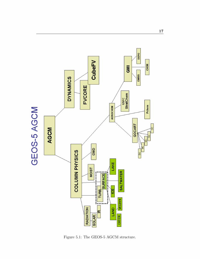
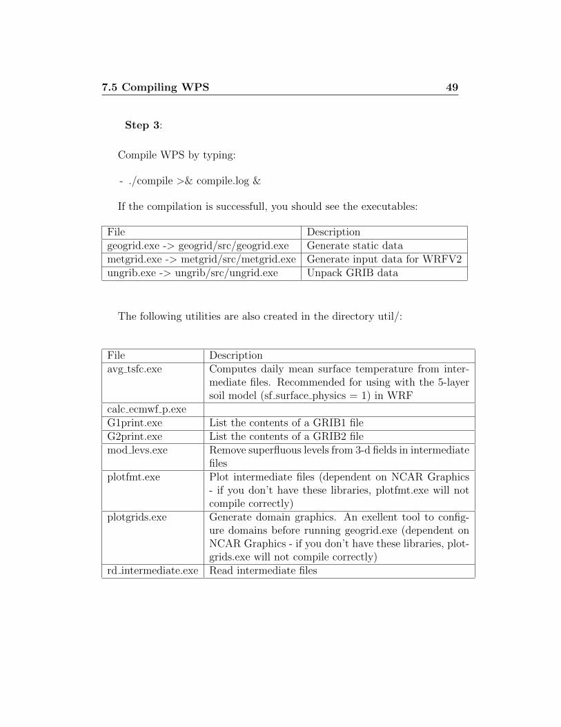
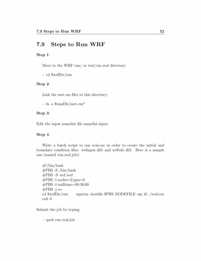
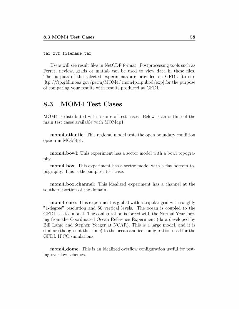Contents

1 System Overview 5

11 Toolkit platform hardware 5


2 NASA Modeling Guru Knowledge Base and Forums 8

3 Torque Scheduler 11

4 NASA Workflow Tool 13

41 Tools and Data 13

42 General Operations 13

43 User Setup 14


5 GEOS-5 AGCM 16


511 MERRA vs Fortuna Tags 18

512 Baselibs 19




541 RC Files 26


CONTENTS 3

56 Case Study 28









64 Visualization 37



651 Case Study 42

7 WRF 43

71 Introduction 43





74 Compiling WRF 46

75 Compiling WPS 47







8 GFDL MOM4 55

CONTENTS 4


811 Solo Models 56





9 FAQ and tips 61



Chapter 1

System Overview










ndash 24gb RAM














Chapter 2










9






10


Chapter 3

Torque Scheduler







PBS -S binbash

PBS -N somejobname

PBS -l nodes=2ppn=8



12



headnodecx1





node-7cx1




Chapter 4

NASA Workflow Tool

41 Tools and Data








43 User Setup 14



nedserverNohuplog







43 User Setup







Chapter 5

GEOS-5 AGCM





17

















512 Baselibs




- C compiler


- GNU make






setenv CVS_RSH ssh










To install












source g5_modules




module list

and you should see


1) compintel-111















cd ssh

ssh-keygen -t dsa




ssh-keygen -t dsa





cd AGCMsetup

EDIT optionsrc file

RUN setupg5gcm



gcm_setup






72 46 (~ 4 -deg)

144 91 (~ 2 -deg)

288 181 (~ 1 -deg)

576 361 (~12-deg)

1152 721 (~14-deg)














umask 022

unlimit









541 RC Files


AGCMrc








AEROCLIMYEAR 2002









AEROCLIMYEAR 2002




HISTORYrc












CAPrc


cap restart


19991231 210000



55 Output and Plots










56 Case Study


56 Case Study 29






Chapter 6

NASA-GISS ModelE






- C compiler













export CVS_RSH=ssh

cvs co modelE








gmake config



Directory structure






specific runs



















OUTPUT_TO_FILES=YES



suppressed

VERBOSE_OUTPUT=YES



COMPILER=intel


mpiltMPIDISTRgtmk

MPIDISTR=mvapich2



ESMF

ESMF=NO

ESMF_COMM=mpich2

ESMF_BOPT=O







MP=NO


















Parallel Build


















64 Visualization 37




ampINPUTZ





ampINPUTZ




64 Visualization



64 Visualization 38





ampampPARAMETERS


ampINPUTZ


ampEND








64 Visualization 39


























then

cd modelEscratch


baselibs

cmrun

decks

etc

exec

input

modelE

optionsrc

out

README

setupmodelE



NETCDFDIR

ESMFDIR

DECK E1M20

COMPILER intel

MPI mvapich2








cd modelEdecks




qsub modele_runj


qstat






651 Case Study



Chapter 7

WRF

71 Introduction

















- WRFV3TARgz

- WPSTARgz



mkdir myWorkDir



Now untar the files

- cd workDir



- tar xvfz WPSTARgz


- for csh



- for bash












74 Compiling WRF 46

NetCDF Library







module load mkl1012





NCL Library




74 Compiling WRF

- cd $wrfDir

Step 1

- configure




75 Compiling WPS 47

Step 2



Step 3








75 Compiling WPS

cd $wpsDir

Step 1

75 Compiling WPS 48

- configure



Step 2


-LusrX11R6lib -lX11

with









with







-lncarg_c



75 Compiling WPS 49

Step 3


















- geogridexe



Step 1



Step 2




- GRIBFILEAAA

- GRIBFILEAAB


- GRIBFILEAAC

- GRIBFILEAAD

- GRIBFILEAAE

- GRIBFILEAAF

Step 3

Run UNGRIB



- FILE2010-02-05 00

- FILE2010-02-05 03

- FILE2010-02-05 06

- FILE2010-02-05 09

- FILE2010-02-05 12


Run METGRID

- metgridexe





79 Steps to Run WRF

Step 1


- cd $wrfDirrun

Step 2



Step 3


Step 4




- qsub run realjob


Step 5





- qsub run wrfjob





48 hour simulation





28 Vertical Levels


711 Run Case Study






cd run


Submit WRF script

qsub run_wrfjob


Chapter 8

GFDL MOM4







ROOT




811 Solo Models












812 Coupled Models













tar xvf filenametar


83 MOM4 Test Cases


















EXPNAME atlantic1

COMPILER ia64

MPI mvapich2




options mom4p1_ebm

mom4p1_coupled

CM21p1_dynamic]


torus1 gyre1

mk3p51]








Chapter 9

FAQ and tips



Bibliography





System Overview




Torque Scheduler

NASA Workflow Tool

Tools and Data

General Operations

User Setup


GEOS-5 AGCM



Baselibs




RC Files

Output and Plots

Case Study

NASA-GISS modelE

System requirements


Getting the code

configuring modelE

Model installation



Visualization


Stand-alone Package

Case Study

WRF

Introduction

Obtaining the Code



Initial Settings

Compiling WRF

Compiling WPS


Steps to Run Ungrib


Steps to Run WRF


Run Case Study

GFDL MOM4


Solo Models

Coupled Models



MOM4 Test Cases

FAQ and tips

Compiler settings


CONTENTS 3

56 Case Study 28









64 Visualization 37



651 Case Study 42

7 WRF 43

71 Introduction 43





74 Compiling WRF 46

75 Compiling WPS 47







8 GFDL MOM4 55

CONTENTS 4


811 Solo Models 56





9 FAQ and tips 61



Chapter 1

System Overview










ndash 24gb RAM














Chapter 2










9






10


Chapter 3

Torque Scheduler







PBS -S binbash

PBS -N somejobname

PBS -l nodes=2ppn=8



12



headnodecx1





node-7cx1




Chapter 4

NASA Workflow Tool

41 Tools and Data








43 User Setup 14



nedserverNohuplog







43 User Setup







Chapter 5

GEOS-5 AGCM





17

















512 Baselibs




- C compiler


- GNU make






setenv CVS_RSH ssh










To install












source g5_modules




module list

and you should see


1) compintel-111















cd ssh

ssh-keygen -t dsa




ssh-keygen -t dsa





cd AGCMsetup

EDIT optionsrc file

RUN setupg5gcm



gcm_setup






72 46 (~ 4 -deg)

144 91 (~ 2 -deg)

288 181 (~ 1 -deg)

576 361 (~12-deg)

1152 721 (~14-deg)














umask 022

unlimit









541 RC Files


AGCMrc








AEROCLIMYEAR 2002









AEROCLIMYEAR 2002




HISTORYrc












CAPrc


cap restart


19991231 210000



55 Output and Plots










56 Case Study


56 Case Study 29






Chapter 6

NASA-GISS ModelE






- C compiler













export CVS_RSH=ssh

cvs co modelE








gmake config



Directory structure






specific runs



















OUTPUT_TO_FILES=YES



suppressed

VERBOSE_OUTPUT=YES



COMPILER=intel


mpiltMPIDISTRgtmk

MPIDISTR=mvapich2



ESMF

ESMF=NO

ESMF_COMM=mpich2

ESMF_BOPT=O







MP=NO


















Parallel Build


















64 Visualization 37




ampINPUTZ





ampINPUTZ




64 Visualization



64 Visualization 38





ampampPARAMETERS


ampINPUTZ


ampEND








64 Visualization 39


























then

cd modelEscratch


baselibs

cmrun

decks

etc

exec

input

modelE

optionsrc

out

README

setupmodelE



NETCDFDIR

ESMFDIR

DECK E1M20

COMPILER intel

MPI mvapich2








cd modelEdecks




qsub modele_runj


qstat






651 Case Study



Chapter 7

WRF

71 Introduction

















- WRFV3TARgz

- WPSTARgz



mkdir myWorkDir



Now untar the files

- cd workDir



- tar xvfz WPSTARgz


- for csh



- for bash












74 Compiling WRF 46

NetCDF Library







module load mkl1012





NCL Library




74 Compiling WRF

- cd $wrfDir

Step 1

- configure




75 Compiling WPS 47

Step 2



Step 3








75 Compiling WPS

cd $wpsDir

Step 1

75 Compiling WPS 48

- configure



Step 2


-LusrX11R6lib -lX11

with









with







-lncarg_c



75 Compiling WPS 49

Step 3


















- geogridexe



Step 1



Step 2




- GRIBFILEAAA

- GRIBFILEAAB


- GRIBFILEAAC

- GRIBFILEAAD

- GRIBFILEAAE

- GRIBFILEAAF

Step 3

Run UNGRIB



- FILE2010-02-05 00

- FILE2010-02-05 03

- FILE2010-02-05 06

- FILE2010-02-05 09

- FILE2010-02-05 12


Run METGRID

- metgridexe





79 Steps to Run WRF

Step 1


- cd $wrfDirrun

Step 2



Step 3


Step 4




- qsub run realjob


Step 5





- qsub run wrfjob





48 hour simulation





28 Vertical Levels


711 Run Case Study






cd run


Submit WRF script

qsub run_wrfjob


Chapter 8

GFDL MOM4







ROOT




811 Solo Models












812 Coupled Models













tar xvf filenametar


83 MOM4 Test Cases


















EXPNAME atlantic1

COMPILER ia64

MPI mvapich2




options mom4p1_ebm

mom4p1_coupled

CM21p1_dynamic]


torus1 gyre1

mk3p51]








Chapter 9

FAQ and tips



Bibliography





System Overview




Torque Scheduler

NASA Workflow Tool

Tools and Data

General Operations

User Setup


GEOS-5 AGCM



Baselibs




RC Files

Output and Plots

Case Study

NASA-GISS modelE

System requirements


Getting the code

configuring modelE

Model installation



Visualization


Stand-alone Package

Case Study

WRF

Introduction

Obtaining the Code



Initial Settings

Compiling WRF

Compiling WPS


Steps to Run Ungrib


Steps to Run WRF


Run Case Study

GFDL MOM4


Solo Models

Coupled Models



MOM4 Test Cases

FAQ and tips

Compiler settings


CONTENTS 4


811 Solo Models 56





9 FAQ and tips 61



Chapter 1

System Overview










ndash 24gb RAM














Chapter 2










9






10


Chapter 3

Torque Scheduler







PBS -S binbash

PBS -N somejobname

PBS -l nodes=2ppn=8



12



headnodecx1





node-7cx1




Chapter 4

NASA Workflow Tool

41 Tools and Data








43 User Setup 14



nedserverNohuplog







43 User Setup







Chapter 5

GEOS-5 AGCM





17

















512 Baselibs




- C compiler


- GNU make






setenv CVS_RSH ssh










To install












source g5_modules




module list

and you should see


1) compintel-111















cd ssh

ssh-keygen -t dsa




ssh-keygen -t dsa





cd AGCMsetup

EDIT optionsrc file

RUN setupg5gcm



gcm_setup






72 46 (~ 4 -deg)

144 91 (~ 2 -deg)

288 181 (~ 1 -deg)

576 361 (~12-deg)

1152 721 (~14-deg)














umask 022

unlimit









541 RC Files


AGCMrc








AEROCLIMYEAR 2002









AEROCLIMYEAR 2002




HISTORYrc












CAPrc


cap restart


19991231 210000



55 Output and Plots










56 Case Study


56 Case Study 29






Chapter 6

NASA-GISS ModelE






- C compiler













export CVS_RSH=ssh

cvs co modelE








gmake config



Directory structure






specific runs



















OUTPUT_TO_FILES=YES



suppressed

VERBOSE_OUTPUT=YES



COMPILER=intel


mpiltMPIDISTRgtmk

MPIDISTR=mvapich2



ESMF

ESMF=NO

ESMF_COMM=mpich2

ESMF_BOPT=O







MP=NO


















Parallel Build


















64 Visualization 37




ampINPUTZ





ampINPUTZ




64 Visualization



64 Visualization 38





ampampPARAMETERS


ampINPUTZ


ampEND








64 Visualization 39


























then

cd modelEscratch


baselibs

cmrun

decks

etc

exec

input

modelE

optionsrc

out

README

setupmodelE



NETCDFDIR

ESMFDIR

DECK E1M20

COMPILER intel

MPI mvapich2








cd modelEdecks




qsub modele_runj


qstat






651 Case Study



Chapter 7

WRF

71 Introduction

















- WRFV3TARgz

- WPSTARgz



mkdir myWorkDir



Now untar the files

- cd workDir



- tar xvfz WPSTARgz


- for csh



- for bash












74 Compiling WRF 46

NetCDF Library







module load mkl1012





NCL Library




74 Compiling WRF

- cd $wrfDir

Step 1

- configure




75 Compiling WPS 47

Step 2



Step 3








75 Compiling WPS

cd $wpsDir

Step 1

75 Compiling WPS 48

- configure



Step 2


-LusrX11R6lib -lX11

with









with







-lncarg_c



75 Compiling WPS 49

Step 3


















- geogridexe



Step 1



Step 2




- GRIBFILEAAA

- GRIBFILEAAB


- GRIBFILEAAC

- GRIBFILEAAD

- GRIBFILEAAE

- GRIBFILEAAF

Step 3

Run UNGRIB



- FILE2010-02-05 00

- FILE2010-02-05 03

- FILE2010-02-05 06

- FILE2010-02-05 09

- FILE2010-02-05 12


Run METGRID

- metgridexe





79 Steps to Run WRF

Step 1


- cd $wrfDirrun

Step 2



Step 3


Step 4




- qsub run realjob


Step 5





- qsub run wrfjob





48 hour simulation





28 Vertical Levels


711 Run Case Study






cd run


Submit WRF script

qsub run_wrfjob


Chapter 8

GFDL MOM4







ROOT




811 Solo Models












812 Coupled Models













tar xvf filenametar


83 MOM4 Test Cases


















EXPNAME atlantic1

COMPILER ia64

MPI mvapich2




options mom4p1_ebm

mom4p1_coupled

CM21p1_dynamic]


torus1 gyre1

mk3p51]








Chapter 9

FAQ and tips



Bibliography





System Overview




Torque Scheduler

NASA Workflow Tool

Tools and Data

General Operations

User Setup


GEOS-5 AGCM



Baselibs




RC Files

Output and Plots

Case Study

NASA-GISS modelE

System requirements


Getting the code

configuring modelE

Model installation



Visualization


Stand-alone Package

Case Study

WRF

Introduction

Obtaining the Code



Initial Settings

Compiling WRF

Compiling WPS


Steps to Run Ungrib


Steps to Run WRF


Run Case Study

GFDL MOM4


Solo Models

Coupled Models



MOM4 Test Cases

FAQ and tips

Compiler settings


Chapter 1

System Overview










ndash 24gb RAM














Chapter 2










9






10


Chapter 3

Torque Scheduler







PBS -S binbash

PBS -N somejobname

PBS -l nodes=2ppn=8



12



headnodecx1





node-7cx1




Chapter 4

NASA Workflow Tool

41 Tools and Data








43 User Setup 14



nedserverNohuplog







43 User Setup







Chapter 5

GEOS-5 AGCM





17

















512 Baselibs




- C compiler


- GNU make






setenv CVS_RSH ssh










To install












source g5_modules




module list

and you should see


1) compintel-111















cd ssh

ssh-keygen -t dsa




ssh-keygen -t dsa





cd AGCMsetup

EDIT optionsrc file

RUN setupg5gcm



gcm_setup






72 46 (~ 4 -deg)

144 91 (~ 2 -deg)

288 181 (~ 1 -deg)

576 361 (~12-deg)

1152 721 (~14-deg)














umask 022

unlimit









541 RC Files


AGCMrc








AEROCLIMYEAR 2002









AEROCLIMYEAR 2002




HISTORYrc












CAPrc


cap restart


19991231 210000



55 Output and Plots










56 Case Study


56 Case Study 29






Chapter 6

NASA-GISS ModelE






- C compiler













export CVS_RSH=ssh

cvs co modelE








gmake config



Directory structure






specific runs



















OUTPUT_TO_FILES=YES



suppressed

VERBOSE_OUTPUT=YES



COMPILER=intel


mpiltMPIDISTRgtmk

MPIDISTR=mvapich2



ESMF

ESMF=NO

ESMF_COMM=mpich2

ESMF_BOPT=O







MP=NO


















Parallel Build


















64 Visualization 37




ampINPUTZ





ampINPUTZ




64 Visualization



64 Visualization 38





ampampPARAMETERS


ampINPUTZ


ampEND








64 Visualization 39


























then

cd modelEscratch


baselibs

cmrun

decks

etc

exec

input

modelE

optionsrc

out

README

setupmodelE



NETCDFDIR

ESMFDIR

DECK E1M20

COMPILER intel

MPI mvapich2








cd modelEdecks




qsub modele_runj


qstat






651 Case Study



Chapter 7

WRF

71 Introduction

















- WRFV3TARgz

- WPSTARgz



mkdir myWorkDir



Now untar the files

- cd workDir



- tar xvfz WPSTARgz


- for csh



- for bash












74 Compiling WRF 46

NetCDF Library







module load mkl1012





NCL Library




74 Compiling WRF

- cd $wrfDir

Step 1

- configure




75 Compiling WPS 47

Step 2



Step 3








75 Compiling WPS

cd $wpsDir

Step 1

75 Compiling WPS 48

- configure



Step 2


-LusrX11R6lib -lX11

with









with







-lncarg_c



75 Compiling WPS 49

Step 3


















- geogridexe



Step 1



Step 2




- GRIBFILEAAA

- GRIBFILEAAB


- GRIBFILEAAC

- GRIBFILEAAD

- GRIBFILEAAE

- GRIBFILEAAF

Step 3

Run UNGRIB



- FILE2010-02-05 00

- FILE2010-02-05 03

- FILE2010-02-05 06

- FILE2010-02-05 09

- FILE2010-02-05 12


Run METGRID

- metgridexe





79 Steps to Run WRF

Step 1


- cd $wrfDirrun

Step 2



Step 3


Step 4




- qsub run realjob


Step 5





- qsub run wrfjob





48 hour simulation





28 Vertical Levels


711 Run Case Study






cd run


Submit WRF script

qsub run_wrfjob


Chapter 8

GFDL MOM4







ROOT




811 Solo Models












812 Coupled Models













tar xvf filenametar


83 MOM4 Test Cases


















EXPNAME atlantic1

COMPILER ia64

MPI mvapich2




options mom4p1_ebm

mom4p1_coupled

CM21p1_dynamic]


torus1 gyre1

mk3p51]








Chapter 9

FAQ and tips



Bibliography





System Overview




Torque Scheduler

NASA Workflow Tool

Tools and Data

General Operations

User Setup


GEOS-5 AGCM



Baselibs




RC Files

Output and Plots

Case Study

NASA-GISS modelE

System requirements


Getting the code

configuring modelE

Model installation



Visualization


Stand-alone Package

Case Study

WRF

Introduction

Obtaining the Code



Initial Settings

Compiling WRF

Compiling WPS


Steps to Run Ungrib


Steps to Run WRF


Run Case Study

GFDL MOM4


Solo Models

Coupled Models



MOM4 Test Cases

FAQ and tips

Compiler settings





ndash 24gb RAM














Chapter 2










9






10


Chapter 3

Torque Scheduler







PBS -S binbash

PBS -N somejobname

PBS -l nodes=2ppn=8



12



headnodecx1





node-7cx1




Chapter 4

NASA Workflow Tool

41 Tools and Data








43 User Setup 14



nedserverNohuplog







43 User Setup







Chapter 5

GEOS-5 AGCM





17

















512 Baselibs




- C compiler


- GNU make






setenv CVS_RSH ssh










To install












source g5_modules




module list

and you should see


1) compintel-111















cd ssh

ssh-keygen -t dsa




ssh-keygen -t dsa





cd AGCMsetup

EDIT optionsrc file

RUN setupg5gcm



gcm_setup






72 46 (~ 4 -deg)

144 91 (~ 2 -deg)

288 181 (~ 1 -deg)

576 361 (~12-deg)

1152 721 (~14-deg)














umask 022

unlimit









541 RC Files


AGCMrc








AEROCLIMYEAR 2002









AEROCLIMYEAR 2002




HISTORYrc












CAPrc


cap restart


19991231 210000



55 Output and Plots










56 Case Study


56 Case Study 29






Chapter 6

NASA-GISS ModelE






- C compiler













export CVS_RSH=ssh

cvs co modelE








gmake config



Directory structure






specific runs



















OUTPUT_TO_FILES=YES



suppressed

VERBOSE_OUTPUT=YES



COMPILER=intel


mpiltMPIDISTRgtmk

MPIDISTR=mvapich2



ESMF

ESMF=NO

ESMF_COMM=mpich2

ESMF_BOPT=O







MP=NO


















Parallel Build


















64 Visualization 37




ampINPUTZ





ampINPUTZ




64 Visualization



64 Visualization 38





ampampPARAMETERS


ampINPUTZ


ampEND








64 Visualization 39


























then

cd modelEscratch


baselibs

cmrun

decks

etc

exec

input

modelE

optionsrc

out

README

setupmodelE



NETCDFDIR

ESMFDIR

DECK E1M20

COMPILER intel

MPI mvapich2








cd modelEdecks




qsub modele_runj


qstat






651 Case Study



Chapter 7

WRF

71 Introduction

















- WRFV3TARgz

- WPSTARgz



mkdir myWorkDir



Now untar the files

- cd workDir



- tar xvfz WPSTARgz


- for csh



- for bash












74 Compiling WRF 46

NetCDF Library







module load mkl1012





NCL Library




74 Compiling WRF

- cd $wrfDir

Step 1

- configure




75 Compiling WPS 47

Step 2



Step 3








75 Compiling WPS

cd $wpsDir

Step 1

75 Compiling WPS 48

- configure



Step 2


-LusrX11R6lib -lX11

with









with







-lncarg_c



75 Compiling WPS 49

Step 3


















- geogridexe



Step 1



Step 2




- GRIBFILEAAA

- GRIBFILEAAB


- GRIBFILEAAC

- GRIBFILEAAD

- GRIBFILEAAE

- GRIBFILEAAF

Step 3

Run UNGRIB



- FILE2010-02-05 00

- FILE2010-02-05 03

- FILE2010-02-05 06

- FILE2010-02-05 09

- FILE2010-02-05 12


Run METGRID

- metgridexe





79 Steps to Run WRF

Step 1


- cd $wrfDirrun

Step 2



Step 3


Step 4




- qsub run realjob


Step 5





- qsub run wrfjob





48 hour simulation





28 Vertical Levels


711 Run Case Study






cd run


Submit WRF script

qsub run_wrfjob


Chapter 8

GFDL MOM4







ROOT




811 Solo Models












812 Coupled Models













tar xvf filenametar


83 MOM4 Test Cases


















EXPNAME atlantic1

COMPILER ia64

MPI mvapich2




options mom4p1_ebm

mom4p1_coupled

CM21p1_dynamic]


torus1 gyre1

mk3p51]








Chapter 9

FAQ and tips



Bibliography





System Overview




Torque Scheduler

NASA Workflow Tool

Tools and Data

General Operations

User Setup


GEOS-5 AGCM



Baselibs




RC Files

Output and Plots

Case Study

NASA-GISS modelE

System requirements


Getting the code

configuring modelE

Model installation



Visualization


Stand-alone Package

Case Study

WRF

Introduction

Obtaining the Code



Initial Settings

Compiling WRF

Compiling WPS


Steps to Run Ungrib


Steps to Run WRF


Run Case Study

GFDL MOM4


Solo Models

Coupled Models



MOM4 Test Cases

FAQ and tips

Compiler settings





Chapter 2










9






10


Chapter 3

Torque Scheduler







PBS -S binbash

PBS -N somejobname

PBS -l nodes=2ppn=8



12



headnodecx1





node-7cx1




Chapter 4

NASA Workflow Tool

41 Tools and Data








43 User Setup 14



nedserverNohuplog







43 User Setup







Chapter 5

GEOS-5 AGCM





17

















512 Baselibs




- C compiler


- GNU make






setenv CVS_RSH ssh










To install












source g5_modules




module list

and you should see


1) compintel-111















cd ssh

ssh-keygen -t dsa




ssh-keygen -t dsa





cd AGCMsetup

EDIT optionsrc file

RUN setupg5gcm



gcm_setup






72 46 (~ 4 -deg)

144 91 (~ 2 -deg)

288 181 (~ 1 -deg)

576 361 (~12-deg)

1152 721 (~14-deg)














umask 022

unlimit









541 RC Files


AGCMrc








AEROCLIMYEAR 2002









AEROCLIMYEAR 2002




HISTORYrc












CAPrc


cap restart


19991231 210000



55 Output and Plots










56 Case Study


56 Case Study 29






Chapter 6

NASA-GISS ModelE






- C compiler













export CVS_RSH=ssh

cvs co modelE








gmake config



Directory structure






specific runs



















OUTPUT_TO_FILES=YES



suppressed

VERBOSE_OUTPUT=YES



COMPILER=intel


mpiltMPIDISTRgtmk

MPIDISTR=mvapich2



ESMF

ESMF=NO

ESMF_COMM=mpich2

ESMF_BOPT=O







MP=NO


















Parallel Build


















64 Visualization 37




ampINPUTZ





ampINPUTZ




64 Visualization



64 Visualization 38





ampampPARAMETERS


ampINPUTZ


ampEND








64 Visualization 39


























then

cd modelEscratch


baselibs

cmrun

decks

etc

exec

input

modelE

optionsrc

out

README

setupmodelE



NETCDFDIR

ESMFDIR

DECK E1M20

COMPILER intel

MPI mvapich2








cd modelEdecks




qsub modele_runj


qstat






651 Case Study



Chapter 7

WRF

71 Introduction

















- WRFV3TARgz

- WPSTARgz



mkdir myWorkDir



Now untar the files

- cd workDir



- tar xvfz WPSTARgz


- for csh



- for bash












74 Compiling WRF 46

NetCDF Library







module load mkl1012





NCL Library




74 Compiling WRF

- cd $wrfDir

Step 1

- configure




75 Compiling WPS 47

Step 2



Step 3








75 Compiling WPS

cd $wpsDir

Step 1

75 Compiling WPS 48

- configure



Step 2


-LusrX11R6lib -lX11

with









with







-lncarg_c



75 Compiling WPS 49

Step 3


















- geogridexe



Step 1



Step 2




- GRIBFILEAAA

- GRIBFILEAAB


- GRIBFILEAAC

- GRIBFILEAAD

- GRIBFILEAAE

- GRIBFILEAAF

Step 3

Run UNGRIB



- FILE2010-02-05 00

- FILE2010-02-05 03

- FILE2010-02-05 06

- FILE2010-02-05 09

- FILE2010-02-05 12


Run METGRID

- metgridexe





79 Steps to Run WRF

Step 1


- cd $wrfDirrun

Step 2



Step 3


Step 4




- qsub run realjob


Step 5





- qsub run wrfjob





48 hour simulation





28 Vertical Levels


711 Run Case Study






cd run


Submit WRF script

qsub run_wrfjob


Chapter 8

GFDL MOM4







ROOT




811 Solo Models












812 Coupled Models













tar xvf filenametar


83 MOM4 Test Cases


















EXPNAME atlantic1

COMPILER ia64

MPI mvapich2




options mom4p1_ebm

mom4p1_coupled

CM21p1_dynamic]


torus1 gyre1

mk3p51]








Chapter 9

FAQ and tips



Bibliography





System Overview




Torque Scheduler

NASA Workflow Tool

Tools and Data

General Operations

User Setup


GEOS-5 AGCM



Baselibs




RC Files

Output and Plots

Case Study

NASA-GISS modelE

System requirements


Getting the code

configuring modelE

Model installation



Visualization


Stand-alone Package

Case Study

WRF

Introduction

Obtaining the Code



Initial Settings

Compiling WRF

Compiling WPS


Steps to Run Ungrib


Steps to Run WRF


Run Case Study

GFDL MOM4


Solo Models

Coupled Models



MOM4 Test Cases

FAQ and tips

Compiler settings


9






10


Chapter 3

Torque Scheduler







PBS -S binbash

PBS -N somejobname

PBS -l nodes=2ppn=8



12



headnodecx1





node-7cx1




Chapter 4

NASA Workflow Tool

41 Tools and Data








43 User Setup 14



nedserverNohuplog







43 User Setup







Chapter 5

GEOS-5 AGCM





17

















512 Baselibs




- C compiler


- GNU make






setenv CVS_RSH ssh










To install












source g5_modules




module list

and you should see


1) compintel-111















cd ssh

ssh-keygen -t dsa




ssh-keygen -t dsa





cd AGCMsetup

EDIT optionsrc file

RUN setupg5gcm



gcm_setup






72 46 (~ 4 -deg)

144 91 (~ 2 -deg)

288 181 (~ 1 -deg)

576 361 (~12-deg)

1152 721 (~14-deg)














umask 022

unlimit









541 RC Files


AGCMrc








AEROCLIMYEAR 2002









AEROCLIMYEAR 2002




HISTORYrc












CAPrc


cap restart


19991231 210000



55 Output and Plots










56 Case Study


56 Case Study 29






Chapter 6

NASA-GISS ModelE






- C compiler













export CVS_RSH=ssh

cvs co modelE








gmake config



Directory structure






specific runs



















OUTPUT_TO_FILES=YES



suppressed

VERBOSE_OUTPUT=YES



COMPILER=intel


mpiltMPIDISTRgtmk

MPIDISTR=mvapich2



ESMF

ESMF=NO

ESMF_COMM=mpich2

ESMF_BOPT=O







MP=NO


















Parallel Build


















64 Visualization 37




ampINPUTZ





ampINPUTZ




64 Visualization



64 Visualization 38





ampampPARAMETERS


ampINPUTZ


ampEND








64 Visualization 39


























then

cd modelEscratch


baselibs

cmrun

decks

etc

exec

input

modelE

optionsrc

out

README

setupmodelE



NETCDFDIR

ESMFDIR

DECK E1M20

COMPILER intel

MPI mvapich2








cd modelEdecks




qsub modele_runj


qstat






651 Case Study



Chapter 7

WRF

71 Introduction

















- WRFV3TARgz

- WPSTARgz



mkdir myWorkDir



Now untar the files

- cd workDir



- tar xvfz WPSTARgz


- for csh



- for bash












74 Compiling WRF 46

NetCDF Library







module load mkl1012





NCL Library




74 Compiling WRF

- cd $wrfDir

Step 1

- configure




75 Compiling WPS 47

Step 2



Step 3








75 Compiling WPS

cd $wpsDir

Step 1

75 Compiling WPS 48

- configure



Step 2


-LusrX11R6lib -lX11

with









with







-lncarg_c



75 Compiling WPS 49

Step 3


















- geogridexe



Step 1



Step 2




- GRIBFILEAAA

- GRIBFILEAAB


- GRIBFILEAAC

- GRIBFILEAAD

- GRIBFILEAAE

- GRIBFILEAAF

Step 3

Run UNGRIB



- FILE2010-02-05 00

- FILE2010-02-05 03

- FILE2010-02-05 06

- FILE2010-02-05 09

- FILE2010-02-05 12


Run METGRID

- metgridexe





79 Steps to Run WRF

Step 1


- cd $wrfDirrun

Step 2



Step 3


Step 4




- qsub run realjob


Step 5





- qsub run wrfjob





48 hour simulation





28 Vertical Levels


711 Run Case Study






cd run


Submit WRF script

qsub run_wrfjob


Chapter 8

GFDL MOM4







ROOT




811 Solo Models












812 Coupled Models













tar xvf filenametar


83 MOM4 Test Cases


















EXPNAME atlantic1

COMPILER ia64

MPI mvapich2




options mom4p1_ebm

mom4p1_coupled

CM21p1_dynamic]


torus1 gyre1

mk3p51]








Chapter 9

FAQ and tips



Bibliography





System Overview




Torque Scheduler

NASA Workflow Tool

Tools and Data

General Operations

User Setup


GEOS-5 AGCM



Baselibs




RC Files

Output and Plots

Case Study

NASA-GISS modelE

System requirements


Getting the code

configuring modelE

Model installation



Visualization


Stand-alone Package

Case Study

WRF

Introduction

Obtaining the Code



Initial Settings

Compiling WRF

Compiling WPS


Steps to Run Ungrib


Steps to Run WRF


Run Case Study

GFDL MOM4


Solo Models

Coupled Models



MOM4 Test Cases

FAQ and tips

Compiler settings


10


Chapter 3

Torque Scheduler







PBS -S binbash

PBS -N somejobname

PBS -l nodes=2ppn=8



12



headnodecx1





node-7cx1




Chapter 4

NASA Workflow Tool

41 Tools and Data








43 User Setup 14



nedserverNohuplog







43 User Setup







Chapter 5

GEOS-5 AGCM





17

















512 Baselibs




- C compiler


- GNU make






setenv CVS_RSH ssh










To install












source g5_modules




module list

and you should see


1) compintel-111















cd ssh

ssh-keygen -t dsa




ssh-keygen -t dsa





cd AGCMsetup

EDIT optionsrc file

RUN setupg5gcm



gcm_setup






72 46 (~ 4 -deg)

144 91 (~ 2 -deg)

288 181 (~ 1 -deg)

576 361 (~12-deg)

1152 721 (~14-deg)














umask 022

unlimit









541 RC Files


AGCMrc








AEROCLIMYEAR 2002









AEROCLIMYEAR 2002




HISTORYrc












CAPrc


cap restart


19991231 210000



55 Output and Plots










56 Case Study


56 Case Study 29






Chapter 6

NASA-GISS ModelE






- C compiler













export CVS_RSH=ssh

cvs co modelE








gmake config



Directory structure






specific runs



















OUTPUT_TO_FILES=YES



suppressed

VERBOSE_OUTPUT=YES



COMPILER=intel


mpiltMPIDISTRgtmk

MPIDISTR=mvapich2



ESMF

ESMF=NO

ESMF_COMM=mpich2

ESMF_BOPT=O







MP=NO


















Parallel Build


















64 Visualization 37




ampINPUTZ





ampINPUTZ




64 Visualization



64 Visualization 38





ampampPARAMETERS


ampINPUTZ


ampEND








64 Visualization 39


























then

cd modelEscratch


baselibs

cmrun

decks

etc

exec

input

modelE

optionsrc

out

README

setupmodelE



NETCDFDIR

ESMFDIR

DECK E1M20

COMPILER intel

MPI mvapich2








cd modelEdecks




qsub modele_runj


qstat






651 Case Study



Chapter 7

WRF

71 Introduction

















- WRFV3TARgz

- WPSTARgz



mkdir myWorkDir



Now untar the files

- cd workDir



- tar xvfz WPSTARgz


- for csh



- for bash












74 Compiling WRF 46

NetCDF Library







module load mkl1012





NCL Library




74 Compiling WRF

- cd $wrfDir

Step 1

- configure




75 Compiling WPS 47

Step 2



Step 3








75 Compiling WPS

cd $wpsDir

Step 1

75 Compiling WPS 48

- configure



Step 2


-LusrX11R6lib -lX11

with









with







-lncarg_c



75 Compiling WPS 49

Step 3


















- geogridexe



Step 1



Step 2




- GRIBFILEAAA

- GRIBFILEAAB


- GRIBFILEAAC

- GRIBFILEAAD

- GRIBFILEAAE

- GRIBFILEAAF

Step 3

Run UNGRIB



- FILE2010-02-05 00

- FILE2010-02-05 03

- FILE2010-02-05 06

- FILE2010-02-05 09

- FILE2010-02-05 12


Run METGRID

- metgridexe





79 Steps to Run WRF

Step 1


- cd $wrfDirrun

Step 2



Step 3


Step 4




- qsub run realjob


Step 5





- qsub run wrfjob





48 hour simulation





28 Vertical Levels


711 Run Case Study






cd run


Submit WRF script

qsub run_wrfjob


Chapter 8

GFDL MOM4







ROOT




811 Solo Models












812 Coupled Models













tar xvf filenametar


83 MOM4 Test Cases


















EXPNAME atlantic1

COMPILER ia64

MPI mvapich2




options mom4p1_ebm

mom4p1_coupled

CM21p1_dynamic]


torus1 gyre1

mk3p51]








Chapter 9

FAQ and tips



Bibliography





System Overview




Torque Scheduler

NASA Workflow Tool

Tools and Data

General Operations

User Setup


GEOS-5 AGCM



Baselibs




RC Files

Output and Plots

Case Study

NASA-GISS modelE

System requirements


Getting the code

configuring modelE

Model installation



Visualization


Stand-alone Package

Case Study

WRF

Introduction

Obtaining the Code



Initial Settings

Compiling WRF

Compiling WPS


Steps to Run Ungrib


Steps to Run WRF


Run Case Study

GFDL MOM4


Solo Models

Coupled Models



MOM4 Test Cases

FAQ and tips

Compiler settings


Chapter 3

Torque Scheduler







PBS -S binbash

PBS -N somejobname

PBS -l nodes=2ppn=8



12



headnodecx1





node-7cx1




Chapter 4

NASA Workflow Tool

41 Tools and Data








43 User Setup 14



nedserverNohuplog







43 User Setup







Chapter 5

GEOS-5 AGCM





17

















512 Baselibs




- C compiler


- GNU make






setenv CVS_RSH ssh










To install












source g5_modules




module list

and you should see


1) compintel-111















cd ssh

ssh-keygen -t dsa




ssh-keygen -t dsa





cd AGCMsetup

EDIT optionsrc file

RUN setupg5gcm



gcm_setup






72 46 (~ 4 -deg)

144 91 (~ 2 -deg)

288 181 (~ 1 -deg)

576 361 (~12-deg)

1152 721 (~14-deg)














umask 022

unlimit









541 RC Files


AGCMrc








AEROCLIMYEAR 2002









AEROCLIMYEAR 2002




HISTORYrc












CAPrc


cap restart


19991231 210000



55 Output and Plots










56 Case Study


56 Case Study 29






Chapter 6

NASA-GISS ModelE






- C compiler













export CVS_RSH=ssh

cvs co modelE








gmake config



Directory structure






specific runs



















OUTPUT_TO_FILES=YES



suppressed

VERBOSE_OUTPUT=YES



COMPILER=intel


mpiltMPIDISTRgtmk

MPIDISTR=mvapich2



ESMF

ESMF=NO

ESMF_COMM=mpich2

ESMF_BOPT=O







MP=NO


















Parallel Build


















64 Visualization 37




ampINPUTZ





ampINPUTZ




64 Visualization



64 Visualization 38





ampampPARAMETERS


ampINPUTZ


ampEND








64 Visualization 39


























then

cd modelEscratch


baselibs

cmrun

decks

etc

exec

input

modelE

optionsrc

out

README

setupmodelE



NETCDFDIR

ESMFDIR

DECK E1M20

COMPILER intel

MPI mvapich2








cd modelEdecks




qsub modele_runj


qstat






651 Case Study



Chapter 7

WRF

71 Introduction

















- WRFV3TARgz

- WPSTARgz



mkdir myWorkDir



Now untar the files

- cd workDir



- tar xvfz WPSTARgz


- for csh



- for bash












74 Compiling WRF 46

NetCDF Library







module load mkl1012





NCL Library




74 Compiling WRF

- cd $wrfDir

Step 1

- configure




75 Compiling WPS 47

Step 2



Step 3








75 Compiling WPS

cd $wpsDir

Step 1

75 Compiling WPS 48

- configure



Step 2


-LusrX11R6lib -lX11

with









with







-lncarg_c



75 Compiling WPS 49

Step 3


















- geogridexe



Step 1



Step 2




- GRIBFILEAAA

- GRIBFILEAAB


- GRIBFILEAAC

- GRIBFILEAAD

- GRIBFILEAAE

- GRIBFILEAAF

Step 3

Run UNGRIB



- FILE2010-02-05 00

- FILE2010-02-05 03

- FILE2010-02-05 06

- FILE2010-02-05 09

- FILE2010-02-05 12


Run METGRID

- metgridexe





79 Steps to Run WRF

Step 1


- cd $wrfDirrun

Step 2



Step 3


Step 4




- qsub run realjob


Step 5





- qsub run wrfjob





48 hour simulation





28 Vertical Levels


711 Run Case Study






cd run


Submit WRF script

qsub run_wrfjob


Chapter 8

GFDL MOM4







ROOT




811 Solo Models












812 Coupled Models













tar xvf filenametar


83 MOM4 Test Cases


















EXPNAME atlantic1

COMPILER ia64

MPI mvapich2




options mom4p1_ebm

mom4p1_coupled

CM21p1_dynamic]


torus1 gyre1

mk3p51]








Chapter 9

FAQ and tips



Bibliography





System Overview




Torque Scheduler

NASA Workflow Tool

Tools and Data

General Operations

User Setup


GEOS-5 AGCM



Baselibs




RC Files

Output and Plots

Case Study

NASA-GISS modelE

System requirements


Getting the code

configuring modelE

Model installation



Visualization


Stand-alone Package

Case Study

WRF

Introduction

Obtaining the Code



Initial Settings

Compiling WRF

Compiling WPS


Steps to Run Ungrib


Steps to Run WRF


Run Case Study

GFDL MOM4


Solo Models

Coupled Models



MOM4 Test Cases

FAQ and tips

Compiler settings


12



headnodecx1





node-7cx1




Chapter 4

NASA Workflow Tool

41 Tools and Data








43 User Setup 14



nedserverNohuplog







43 User Setup







Chapter 5

GEOS-5 AGCM





17

















512 Baselibs




- C compiler


- GNU make






setenv CVS_RSH ssh










To install












source g5_modules




module list

and you should see


1) compintel-111















cd ssh

ssh-keygen -t dsa




ssh-keygen -t dsa





cd AGCMsetup

EDIT optionsrc file

RUN setupg5gcm



gcm_setup






72 46 (~ 4 -deg)

144 91 (~ 2 -deg)

288 181 (~ 1 -deg)

576 361 (~12-deg)

1152 721 (~14-deg)














umask 022

unlimit









541 RC Files


AGCMrc








AEROCLIMYEAR 2002









AEROCLIMYEAR 2002




HISTORYrc












CAPrc


cap restart


19991231 210000



55 Output and Plots










56 Case Study


56 Case Study 29






Chapter 6

NASA-GISS ModelE






- C compiler













export CVS_RSH=ssh

cvs co modelE








gmake config



Directory structure






specific runs



















OUTPUT_TO_FILES=YES



suppressed

VERBOSE_OUTPUT=YES



COMPILER=intel


mpiltMPIDISTRgtmk

MPIDISTR=mvapich2



ESMF

ESMF=NO

ESMF_COMM=mpich2

ESMF_BOPT=O







MP=NO


















Parallel Build


















64 Visualization 37




ampINPUTZ





ampINPUTZ




64 Visualization



64 Visualization 38





ampampPARAMETERS


ampINPUTZ


ampEND








64 Visualization 39


























then

cd modelEscratch


baselibs

cmrun

decks

etc

exec

input

modelE

optionsrc

out

README

setupmodelE



NETCDFDIR

ESMFDIR

DECK E1M20

COMPILER intel

MPI mvapich2








cd modelEdecks




qsub modele_runj


qstat






651 Case Study



Chapter 7

WRF

71 Introduction

















- WRFV3TARgz

- WPSTARgz



mkdir myWorkDir



Now untar the files

- cd workDir



- tar xvfz WPSTARgz


- for csh



- for bash












74 Compiling WRF 46

NetCDF Library







module load mkl1012





NCL Library




74 Compiling WRF

- cd $wrfDir

Step 1

- configure




75 Compiling WPS 47

Step 2



Step 3








75 Compiling WPS

cd $wpsDir

Step 1

75 Compiling WPS 48

- configure



Step 2


-LusrX11R6lib -lX11

with









with







-lncarg_c



75 Compiling WPS 49

Step 3


















- geogridexe



Step 1



Step 2




- GRIBFILEAAA

- GRIBFILEAAB


- GRIBFILEAAC

- GRIBFILEAAD

- GRIBFILEAAE

- GRIBFILEAAF

Step 3

Run UNGRIB



- FILE2010-02-05 00

- FILE2010-02-05 03

- FILE2010-02-05 06

- FILE2010-02-05 09

- FILE2010-02-05 12


Run METGRID

- metgridexe





79 Steps to Run WRF

Step 1


- cd $wrfDirrun

Step 2



Step 3


Step 4




- qsub run realjob


Step 5





- qsub run wrfjob





48 hour simulation





28 Vertical Levels


711 Run Case Study






cd run


Submit WRF script

qsub run_wrfjob


Chapter 8

GFDL MOM4







ROOT




811 Solo Models












812 Coupled Models













tar xvf filenametar


83 MOM4 Test Cases


















EXPNAME atlantic1

COMPILER ia64

MPI mvapich2




options mom4p1_ebm

mom4p1_coupled

CM21p1_dynamic]


torus1 gyre1

mk3p51]








Chapter 9

FAQ and tips



Bibliography





System Overview




Torque Scheduler

NASA Workflow Tool

Tools and Data

General Operations

User Setup


GEOS-5 AGCM



Baselibs




RC Files

Output and Plots

Case Study

NASA-GISS modelE

System requirements


Getting the code

configuring modelE

Model installation



Visualization


Stand-alone Package

Case Study

WRF

Introduction

Obtaining the Code



Initial Settings

Compiling WRF

Compiling WPS


Steps to Run Ungrib


Steps to Run WRF


Run Case Study

GFDL MOM4


Solo Models

Coupled Models



MOM4 Test Cases

FAQ and tips

Compiler settings


Chapter 4

NASA Workflow Tool

41 Tools and Data








43 User Setup 14



nedserverNohuplog







43 User Setup







Chapter 5

GEOS-5 AGCM





17

















512 Baselibs




- C compiler


- GNU make






setenv CVS_RSH ssh










To install












source g5_modules




module list

and you should see


1) compintel-111















cd ssh

ssh-keygen -t dsa




ssh-keygen -t dsa





cd AGCMsetup

EDIT optionsrc file

RUN setupg5gcm



gcm_setup






72 46 (~ 4 -deg)

144 91 (~ 2 -deg)

288 181 (~ 1 -deg)

576 361 (~12-deg)

1152 721 (~14-deg)














umask 022

unlimit









541 RC Files


AGCMrc








AEROCLIMYEAR 2002









AEROCLIMYEAR 2002




HISTORYrc












CAPrc


cap restart


19991231 210000



55 Output and Plots










56 Case Study


56 Case Study 29






Chapter 6

NASA-GISS ModelE






- C compiler













export CVS_RSH=ssh

cvs co modelE








gmake config



Directory structure






specific runs



















OUTPUT_TO_FILES=YES



suppressed

VERBOSE_OUTPUT=YES



COMPILER=intel


mpiltMPIDISTRgtmk

MPIDISTR=mvapich2



ESMF

ESMF=NO

ESMF_COMM=mpich2

ESMF_BOPT=O







MP=NO


















Parallel Build


















64 Visualization 37




ampINPUTZ





ampINPUTZ




64 Visualization



64 Visualization 38





ampampPARAMETERS


ampINPUTZ


ampEND








64 Visualization 39


























then

cd modelEscratch


baselibs

cmrun

decks

etc

exec

input

modelE

optionsrc

out

README

setupmodelE



NETCDFDIR

ESMFDIR

DECK E1M20

COMPILER intel

MPI mvapich2








cd modelEdecks




qsub modele_runj


qstat






651 Case Study



Chapter 7

WRF

71 Introduction

















- WRFV3TARgz

- WPSTARgz



mkdir myWorkDir



Now untar the files

- cd workDir



- tar xvfz WPSTARgz


- for csh



- for bash












74 Compiling WRF 46

NetCDF Library







module load mkl1012





NCL Library




74 Compiling WRF

- cd $wrfDir

Step 1

- configure




75 Compiling WPS 47

Step 2



Step 3








75 Compiling WPS

cd $wpsDir

Step 1

75 Compiling WPS 48

- configure



Step 2


-LusrX11R6lib -lX11

with









with







-lncarg_c



75 Compiling WPS 49

Step 3


















- geogridexe



Step 1



Step 2




- GRIBFILEAAA

- GRIBFILEAAB


- GRIBFILEAAC

- GRIBFILEAAD

- GRIBFILEAAE

- GRIBFILEAAF

Step 3

Run UNGRIB



- FILE2010-02-05 00

- FILE2010-02-05 03

- FILE2010-02-05 06

- FILE2010-02-05 09

- FILE2010-02-05 12


Run METGRID

- metgridexe





79 Steps to Run WRF

Step 1


- cd $wrfDirrun

Step 2



Step 3


Step 4




- qsub run realjob


Step 5





- qsub run wrfjob





48 hour simulation





28 Vertical Levels


711 Run Case Study






cd run


Submit WRF script

qsub run_wrfjob


Chapter 8

GFDL MOM4







ROOT




811 Solo Models












812 Coupled Models













tar xvf filenametar


83 MOM4 Test Cases


















EXPNAME atlantic1

COMPILER ia64

MPI mvapich2




options mom4p1_ebm

mom4p1_coupled

CM21p1_dynamic]


torus1 gyre1

mk3p51]








Chapter 9

FAQ and tips



Bibliography





System Overview




Torque Scheduler

NASA Workflow Tool

Tools and Data

General Operations

User Setup


GEOS-5 AGCM



Baselibs




RC Files

Output and Plots

Case Study

NASA-GISS modelE

System requirements


Getting the code

configuring modelE

Model installation



Visualization


Stand-alone Package

Case Study

WRF

Introduction

Obtaining the Code



Initial Settings

Compiling WRF

Compiling WPS


Steps to Run Ungrib


Steps to Run WRF


Run Case Study

GFDL MOM4


Solo Models

Coupled Models



MOM4 Test Cases

FAQ and tips

Compiler settings


43 User Setup 14



nedserverNohuplog







43 User Setup







Chapter 5

GEOS-5 AGCM





17

















512 Baselibs




- C compiler


- GNU make






setenv CVS_RSH ssh










To install












source g5_modules




module list

and you should see


1) compintel-111















cd ssh

ssh-keygen -t dsa




ssh-keygen -t dsa





cd AGCMsetup

EDIT optionsrc file

RUN setupg5gcm



gcm_setup






72 46 (~ 4 -deg)

144 91 (~ 2 -deg)

288 181 (~ 1 -deg)

576 361 (~12-deg)

1152 721 (~14-deg)














umask 022

unlimit









541 RC Files


AGCMrc








AEROCLIMYEAR 2002









AEROCLIMYEAR 2002




HISTORYrc












CAPrc


cap restart


19991231 210000



55 Output and Plots










56 Case Study


56 Case Study 29






Chapter 6

NASA-GISS ModelE






- C compiler













export CVS_RSH=ssh

cvs co modelE








gmake config



Directory structure






specific runs



















OUTPUT_TO_FILES=YES



suppressed

VERBOSE_OUTPUT=YES



COMPILER=intel


mpiltMPIDISTRgtmk

MPIDISTR=mvapich2



ESMF

ESMF=NO

ESMF_COMM=mpich2

ESMF_BOPT=O







MP=NO


















Parallel Build


















64 Visualization 37




ampINPUTZ





ampINPUTZ




64 Visualization



64 Visualization 38





ampampPARAMETERS


ampINPUTZ


ampEND








64 Visualization 39


























then

cd modelEscratch


baselibs

cmrun

decks

etc

exec

input

modelE

optionsrc

out

README

setupmodelE



NETCDFDIR

ESMFDIR

DECK E1M20

COMPILER intel

MPI mvapich2








cd modelEdecks




qsub modele_runj


qstat






651 Case Study



Chapter 7

WRF

71 Introduction

















- WRFV3TARgz

- WPSTARgz



mkdir myWorkDir



Now untar the files

- cd workDir



- tar xvfz WPSTARgz


- for csh



- for bash












74 Compiling WRF 46

NetCDF Library







module load mkl1012





NCL Library




74 Compiling WRF

- cd $wrfDir

Step 1

- configure




75 Compiling WPS 47

Step 2



Step 3








75 Compiling WPS

cd $wpsDir

Step 1

75 Compiling WPS 48

- configure



Step 2


-LusrX11R6lib -lX11

with









with







-lncarg_c



75 Compiling WPS 49

Step 3


















- geogridexe



Step 1



Step 2




- GRIBFILEAAA

- GRIBFILEAAB


- GRIBFILEAAC

- GRIBFILEAAD

- GRIBFILEAAE

- GRIBFILEAAF

Step 3

Run UNGRIB



- FILE2010-02-05 00

- FILE2010-02-05 03

- FILE2010-02-05 06

- FILE2010-02-05 09

- FILE2010-02-05 12


Run METGRID

- metgridexe





79 Steps to Run WRF

Step 1


- cd $wrfDirrun

Step 2



Step 3


Step 4




- qsub run realjob


Step 5





- qsub run wrfjob





48 hour simulation





28 Vertical Levels


711 Run Case Study






cd run


Submit WRF script

qsub run_wrfjob


Chapter 8

GFDL MOM4







ROOT




811 Solo Models












812 Coupled Models













tar xvf filenametar


83 MOM4 Test Cases


















EXPNAME atlantic1

COMPILER ia64

MPI mvapich2




options mom4p1_ebm

mom4p1_coupled

CM21p1_dynamic]


torus1 gyre1

mk3p51]








Chapter 9

FAQ and tips



Bibliography





System Overview




Torque Scheduler

NASA Workflow Tool

Tools and Data

General Operations

User Setup


GEOS-5 AGCM



Baselibs




RC Files

Output and Plots

Case Study

NASA-GISS modelE

System requirements


Getting the code

configuring modelE

Model installation



Visualization


Stand-alone Package

Case Study

WRF

Introduction

Obtaining the Code



Initial Settings

Compiling WRF

Compiling WPS


Steps to Run Ungrib


Steps to Run WRF


Run Case Study

GFDL MOM4


Solo Models

Coupled Models



MOM4 Test Cases

FAQ and tips

Compiler settings





Chapter 5

GEOS-5 AGCM





17

















512 Baselibs




- C compiler


- GNU make






setenv CVS_RSH ssh










To install












source g5_modules




module list

and you should see


1) compintel-111















cd ssh

ssh-keygen -t dsa




ssh-keygen -t dsa





cd AGCMsetup

EDIT optionsrc file

RUN setupg5gcm



gcm_setup






72 46 (~ 4 -deg)

144 91 (~ 2 -deg)

288 181 (~ 1 -deg)

576 361 (~12-deg)

1152 721 (~14-deg)














umask 022

unlimit









541 RC Files


AGCMrc








AEROCLIMYEAR 2002









AEROCLIMYEAR 2002




HISTORYrc












CAPrc


cap restart


19991231 210000



55 Output and Plots










56 Case Study


56 Case Study 29






Chapter 6

NASA-GISS ModelE






- C compiler













export CVS_RSH=ssh

cvs co modelE








gmake config



Directory structure






specific runs



















OUTPUT_TO_FILES=YES



suppressed

VERBOSE_OUTPUT=YES



COMPILER=intel


mpiltMPIDISTRgtmk

MPIDISTR=mvapich2



ESMF

ESMF=NO

ESMF_COMM=mpich2

ESMF_BOPT=O







MP=NO


















Parallel Build


















64 Visualization 37




ampINPUTZ





ampINPUTZ




64 Visualization



64 Visualization 38





ampampPARAMETERS


ampINPUTZ


ampEND








64 Visualization 39


























then

cd modelEscratch


baselibs

cmrun

decks

etc

exec

input

modelE

optionsrc

out

README

setupmodelE



NETCDFDIR

ESMFDIR

DECK E1M20

COMPILER intel

MPI mvapich2








cd modelEdecks




qsub modele_runj


qstat






651 Case Study



Chapter 7

WRF

71 Introduction

















- WRFV3TARgz

- WPSTARgz



mkdir myWorkDir



Now untar the files

- cd workDir



- tar xvfz WPSTARgz


- for csh



- for bash












74 Compiling WRF 46

NetCDF Library







module load mkl1012





NCL Library




74 Compiling WRF

- cd $wrfDir

Step 1

- configure




75 Compiling WPS 47

Step 2



Step 3








75 Compiling WPS

cd $wpsDir

Step 1

75 Compiling WPS 48

- configure



Step 2


-LusrX11R6lib -lX11

with









with







-lncarg_c



75 Compiling WPS 49

Step 3


















- geogridexe



Step 1



Step 2




- GRIBFILEAAA

- GRIBFILEAAB


- GRIBFILEAAC

- GRIBFILEAAD

- GRIBFILEAAE

- GRIBFILEAAF

Step 3

Run UNGRIB



- FILE2010-02-05 00

- FILE2010-02-05 03

- FILE2010-02-05 06

- FILE2010-02-05 09

- FILE2010-02-05 12


Run METGRID

- metgridexe





79 Steps to Run WRF

Step 1


- cd $wrfDirrun

Step 2



Step 3


Step 4




- qsub run realjob


Step 5





- qsub run wrfjob





48 hour simulation





28 Vertical Levels


711 Run Case Study






cd run


Submit WRF script

qsub run_wrfjob


Chapter 8

GFDL MOM4







ROOT




811 Solo Models












812 Coupled Models













tar xvf filenametar


83 MOM4 Test Cases


















EXPNAME atlantic1

COMPILER ia64

MPI mvapich2




options mom4p1_ebm

mom4p1_coupled

CM21p1_dynamic]


torus1 gyre1

mk3p51]








Chapter 9

FAQ and tips



Bibliography





System Overview




Torque Scheduler

NASA Workflow Tool

Tools and Data

General Operations

User Setup


GEOS-5 AGCM



Baselibs




RC Files

Output and Plots

Case Study

NASA-GISS modelE

System requirements


Getting the code

configuring modelE

Model installation



Visualization


Stand-alone Package

Case Study

WRF

Introduction

Obtaining the Code



Initial Settings

Compiling WRF

Compiling WPS


Steps to Run Ungrib


Steps to Run WRF


Run Case Study

GFDL MOM4


Solo Models

Coupled Models



MOM4 Test Cases

FAQ and tips

Compiler settings


17

















512 Baselibs




- C compiler


- GNU make






setenv CVS_RSH ssh










To install












source g5_modules




module list

and you should see


1) compintel-111















cd ssh

ssh-keygen -t dsa




ssh-keygen -t dsa





cd AGCMsetup

EDIT optionsrc file

RUN setupg5gcm



gcm_setup






72 46 (~ 4 -deg)

144 91 (~ 2 -deg)

288 181 (~ 1 -deg)

576 361 (~12-deg)

1152 721 (~14-deg)














umask 022

unlimit









541 RC Files


AGCMrc








AEROCLIMYEAR 2002









AEROCLIMYEAR 2002




HISTORYrc












CAPrc


cap restart


19991231 210000



55 Output and Plots










56 Case Study


56 Case Study 29






Chapter 6

NASA-GISS ModelE






- C compiler













export CVS_RSH=ssh

cvs co modelE








gmake config



Directory structure






specific runs



















OUTPUT_TO_FILES=YES



suppressed

VERBOSE_OUTPUT=YES



COMPILER=intel


mpiltMPIDISTRgtmk

MPIDISTR=mvapich2



ESMF

ESMF=NO

ESMF_COMM=mpich2

ESMF_BOPT=O







MP=NO


















Parallel Build


















64 Visualization 37




ampINPUTZ





ampINPUTZ




64 Visualization



64 Visualization 38





ampampPARAMETERS


ampINPUTZ


ampEND








64 Visualization 39


























then

cd modelEscratch


baselibs

cmrun

decks

etc

exec

input

modelE

optionsrc

out

README

setupmodelE



NETCDFDIR

ESMFDIR

DECK E1M20

COMPILER intel

MPI mvapich2








cd modelEdecks




qsub modele_runj


qstat






651 Case Study



Chapter 7

WRF

71 Introduction

















- WRFV3TARgz

- WPSTARgz



mkdir myWorkDir



Now untar the files

- cd workDir



- tar xvfz WPSTARgz


- for csh



- for bash












74 Compiling WRF 46

NetCDF Library







module load mkl1012





NCL Library




74 Compiling WRF

- cd $wrfDir

Step 1

- configure




75 Compiling WPS 47

Step 2



Step 3








75 Compiling WPS

cd $wpsDir

Step 1

75 Compiling WPS 48

- configure



Step 2


-LusrX11R6lib -lX11

with









with







-lncarg_c



75 Compiling WPS 49

Step 3


















- geogridexe



Step 1



Step 2




- GRIBFILEAAA

- GRIBFILEAAB


- GRIBFILEAAC

- GRIBFILEAAD

- GRIBFILEAAE

- GRIBFILEAAF

Step 3

Run UNGRIB



- FILE2010-02-05 00

- FILE2010-02-05 03

- FILE2010-02-05 06

- FILE2010-02-05 09

- FILE2010-02-05 12


Run METGRID

- metgridexe





79 Steps to Run WRF

Step 1


- cd $wrfDirrun

Step 2



Step 3


Step 4




- qsub run realjob


Step 5





- qsub run wrfjob





48 hour simulation





28 Vertical Levels


711 Run Case Study






cd run


Submit WRF script

qsub run_wrfjob


Chapter 8

GFDL MOM4







ROOT




811 Solo Models












812 Coupled Models













tar xvf filenametar


83 MOM4 Test Cases


















EXPNAME atlantic1

COMPILER ia64

MPI mvapich2




options mom4p1_ebm

mom4p1_coupled

CM21p1_dynamic]


torus1 gyre1

mk3p51]








Chapter 9

FAQ and tips



Bibliography





System Overview




Torque Scheduler

NASA Workflow Tool

Tools and Data

General Operations

User Setup


GEOS-5 AGCM



Baselibs




RC Files

Output and Plots

Case Study

NASA-GISS modelE

System requirements


Getting the code

configuring modelE

Model installation



Visualization


Stand-alone Package

Case Study

WRF

Introduction

Obtaining the Code



Initial Settings

Compiling WRF

Compiling WPS


Steps to Run Ungrib


Steps to Run WRF


Run Case Study

GFDL MOM4


Solo Models

Coupled Models



MOM4 Test Cases

FAQ and tips

Compiler settings

















512 Baselibs




- C compiler


- GNU make






setenv CVS_RSH ssh










To install












source g5_modules




module list

and you should see


1) compintel-111















cd ssh

ssh-keygen -t dsa




ssh-keygen -t dsa





cd AGCMsetup

EDIT optionsrc file

RUN setupg5gcm



gcm_setup






72 46 (~ 4 -deg)

144 91 (~ 2 -deg)

288 181 (~ 1 -deg)

576 361 (~12-deg)

1152 721 (~14-deg)














umask 022

unlimit









541 RC Files


AGCMrc








AEROCLIMYEAR 2002









AEROCLIMYEAR 2002




HISTORYrc












CAPrc


cap restart


19991231 210000



55 Output and Plots










56 Case Study


56 Case Study 29






Chapter 6

NASA-GISS ModelE






- C compiler













export CVS_RSH=ssh

cvs co modelE








gmake config



Directory structure






specific runs



















OUTPUT_TO_FILES=YES



suppressed

VERBOSE_OUTPUT=YES



COMPILER=intel


mpiltMPIDISTRgtmk

MPIDISTR=mvapich2



ESMF

ESMF=NO

ESMF_COMM=mpich2

ESMF_BOPT=O







MP=NO


















Parallel Build


















64 Visualization 37




ampINPUTZ





ampINPUTZ




64 Visualization



64 Visualization 38





ampampPARAMETERS


ampINPUTZ


ampEND








64 Visualization 39


























then

cd modelEscratch


baselibs

cmrun

decks

etc

exec

input

modelE

optionsrc

out

README

setupmodelE



NETCDFDIR

ESMFDIR

DECK E1M20

COMPILER intel

MPI mvapich2








cd modelEdecks




qsub modele_runj


qstat






651 Case Study



Chapter 7

WRF

71 Introduction

















- WRFV3TARgz

- WPSTARgz



mkdir myWorkDir



Now untar the files

- cd workDir



- tar xvfz WPSTARgz


- for csh



- for bash












74 Compiling WRF 46

NetCDF Library







module load mkl1012





NCL Library




74 Compiling WRF

- cd $wrfDir

Step 1

- configure




75 Compiling WPS 47

Step 2



Step 3








75 Compiling WPS

cd $wpsDir

Step 1

75 Compiling WPS 48

- configure



Step 2


-LusrX11R6lib -lX11

with









with







-lncarg_c



75 Compiling WPS 49

Step 3


















- geogridexe



Step 1



Step 2




- GRIBFILEAAA

- GRIBFILEAAB


- GRIBFILEAAC

- GRIBFILEAAD

- GRIBFILEAAE

- GRIBFILEAAF

Step 3

Run UNGRIB



- FILE2010-02-05 00

- FILE2010-02-05 03

- FILE2010-02-05 06

- FILE2010-02-05 09

- FILE2010-02-05 12


Run METGRID

- metgridexe





79 Steps to Run WRF

Step 1


- cd $wrfDirrun

Step 2



Step 3


Step 4




- qsub run realjob


Step 5





- qsub run wrfjob





48 hour simulation





28 Vertical Levels


711 Run Case Study






cd run


Submit WRF script

qsub run_wrfjob


Chapter 8

GFDL MOM4







ROOT




811 Solo Models












812 Coupled Models













tar xvf filenametar


83 MOM4 Test Cases


















EXPNAME atlantic1

COMPILER ia64

MPI mvapich2




options mom4p1_ebm

mom4p1_coupled

CM21p1_dynamic]


torus1 gyre1

mk3p51]








Chapter 9

FAQ and tips



Bibliography





System Overview




Torque Scheduler

NASA Workflow Tool

Tools and Data

General Operations

User Setup


GEOS-5 AGCM



Baselibs




RC Files

Output and Plots

Case Study

NASA-GISS modelE

System requirements


Getting the code

configuring modelE

Model installation



Visualization


Stand-alone Package

Case Study

WRF

Introduction

Obtaining the Code



Initial Settings

Compiling WRF

Compiling WPS


Steps to Run Ungrib


Steps to Run WRF


Run Case Study

GFDL MOM4


Solo Models

Coupled Models



MOM4 Test Cases

FAQ and tips

Compiler settings









To install












source g5_modules




module list

and you should see


1) compintel-111















cd ssh

ssh-keygen -t dsa




ssh-keygen -t dsa





cd AGCMsetup

EDIT optionsrc file

RUN setupg5gcm



gcm_setup






72 46 (~ 4 -deg)

144 91 (~ 2 -deg)

288 181 (~ 1 -deg)

576 361 (~12-deg)

1152 721 (~14-deg)














umask 022

unlimit









541 RC Files


AGCMrc








AEROCLIMYEAR 2002









AEROCLIMYEAR 2002




HISTORYrc












CAPrc


cap restart


19991231 210000



55 Output and Plots










56 Case Study


56 Case Study 29






Chapter 6

NASA-GISS ModelE






- C compiler













export CVS_RSH=ssh

cvs co modelE








gmake config



Directory structure






specific runs



















OUTPUT_TO_FILES=YES



suppressed

VERBOSE_OUTPUT=YES



COMPILER=intel


mpiltMPIDISTRgtmk

MPIDISTR=mvapich2



ESMF

ESMF=NO

ESMF_COMM=mpich2

ESMF_BOPT=O







MP=NO


















Parallel Build


















64 Visualization 37




ampINPUTZ





ampINPUTZ




64 Visualization



64 Visualization 38





ampampPARAMETERS


ampINPUTZ


ampEND








64 Visualization 39


























then

cd modelEscratch


baselibs

cmrun

decks

etc

exec

input

modelE

optionsrc

out

README

setupmodelE



NETCDFDIR

ESMFDIR

DECK E1M20

COMPILER intel

MPI mvapich2








cd modelEdecks




qsub modele_runj


qstat






651 Case Study



Chapter 7

WRF

71 Introduction

















- WRFV3TARgz

- WPSTARgz



mkdir myWorkDir



Now untar the files

- cd workDir



- tar xvfz WPSTARgz


- for csh



- for bash












74 Compiling WRF 46

NetCDF Library







module load mkl1012





NCL Library




74 Compiling WRF

- cd $wrfDir

Step 1

- configure




75 Compiling WPS 47

Step 2



Step 3








75 Compiling WPS

cd $wpsDir

Step 1

75 Compiling WPS 48

- configure



Step 2


-LusrX11R6lib -lX11

with









with







-lncarg_c



75 Compiling WPS 49

Step 3


















- geogridexe



Step 1



Step 2




- GRIBFILEAAA

- GRIBFILEAAB


- GRIBFILEAAC

- GRIBFILEAAD

- GRIBFILEAAE

- GRIBFILEAAF

Step 3

Run UNGRIB



- FILE2010-02-05 00

- FILE2010-02-05 03

- FILE2010-02-05 06

- FILE2010-02-05 09

- FILE2010-02-05 12


Run METGRID

- metgridexe





79 Steps to Run WRF

Step 1


- cd $wrfDirrun

Step 2



Step 3


Step 4




- qsub run realjob


Step 5





- qsub run wrfjob





48 hour simulation





28 Vertical Levels


711 Run Case Study






cd run


Submit WRF script

qsub run_wrfjob


Chapter 8

GFDL MOM4







ROOT




811 Solo Models












812 Coupled Models













tar xvf filenametar


83 MOM4 Test Cases


















EXPNAME atlantic1

COMPILER ia64

MPI mvapich2




options mom4p1_ebm

mom4p1_coupled

CM21p1_dynamic]


torus1 gyre1

mk3p51]








Chapter 9

FAQ and tips



Bibliography





System Overview




Torque Scheduler

NASA Workflow Tool

Tools and Data

General Operations

User Setup


GEOS-5 AGCM



Baselibs




RC Files

Output and Plots

Case Study

NASA-GISS modelE

System requirements


Getting the code

configuring modelE

Model installation



Visualization


Stand-alone Package

Case Study

WRF

Introduction

Obtaining the Code



Initial Settings

Compiling WRF

Compiling WPS


Steps to Run Ungrib


Steps to Run WRF


Run Case Study

GFDL MOM4


Solo Models

Coupled Models



MOM4 Test Cases

FAQ and tips

Compiler settings






source g5_modules




module list

and you should see


1) compintel-111















cd ssh

ssh-keygen -t dsa




ssh-keygen -t dsa





cd AGCMsetup

EDIT optionsrc file

RUN setupg5gcm



gcm_setup






72 46 (~ 4 -deg)

144 91 (~ 2 -deg)

288 181 (~ 1 -deg)

576 361 (~12-deg)

1152 721 (~14-deg)














umask 022

unlimit









541 RC Files


AGCMrc








AEROCLIMYEAR 2002









AEROCLIMYEAR 2002




HISTORYrc












CAPrc


cap restart


19991231 210000



55 Output and Plots










56 Case Study


56 Case Study 29






Chapter 6

NASA-GISS ModelE






- C compiler













export CVS_RSH=ssh

cvs co modelE








gmake config



Directory structure






specific runs



















OUTPUT_TO_FILES=YES



suppressed

VERBOSE_OUTPUT=YES



COMPILER=intel


mpiltMPIDISTRgtmk

MPIDISTR=mvapich2



ESMF

ESMF=NO

ESMF_COMM=mpich2

ESMF_BOPT=O







MP=NO


















Parallel Build


















64 Visualization 37




ampINPUTZ





ampINPUTZ




64 Visualization



64 Visualization 38





ampampPARAMETERS


ampINPUTZ


ampEND








64 Visualization 39


























then

cd modelEscratch


baselibs

cmrun

decks

etc

exec

input

modelE

optionsrc

out

README

setupmodelE



NETCDFDIR

ESMFDIR

DECK E1M20

COMPILER intel

MPI mvapich2








cd modelEdecks




qsub modele_runj


qstat






651 Case Study



Chapter 7

WRF

71 Introduction

















- WRFV3TARgz

- WPSTARgz



mkdir myWorkDir



Now untar the files

- cd workDir



- tar xvfz WPSTARgz


- for csh



- for bash












74 Compiling WRF 46

NetCDF Library







module load mkl1012





NCL Library




74 Compiling WRF

- cd $wrfDir

Step 1

- configure




75 Compiling WPS 47

Step 2



Step 3








75 Compiling WPS

cd $wpsDir

Step 1

75 Compiling WPS 48

- configure



Step 2


-LusrX11R6lib -lX11

with









with







-lncarg_c



75 Compiling WPS 49

Step 3


















- geogridexe



Step 1



Step 2




- GRIBFILEAAA

- GRIBFILEAAB


- GRIBFILEAAC

- GRIBFILEAAD

- GRIBFILEAAE

- GRIBFILEAAF

Step 3

Run UNGRIB



- FILE2010-02-05 00

- FILE2010-02-05 03

- FILE2010-02-05 06

- FILE2010-02-05 09

- FILE2010-02-05 12


Run METGRID

- metgridexe





79 Steps to Run WRF

Step 1


- cd $wrfDirrun

Step 2



Step 3


Step 4




- qsub run realjob


Step 5





- qsub run wrfjob





48 hour simulation





28 Vertical Levels


711 Run Case Study






cd run


Submit WRF script

qsub run_wrfjob


Chapter 8

GFDL MOM4







ROOT




811 Solo Models












812 Coupled Models













tar xvf filenametar


83 MOM4 Test Cases


















EXPNAME atlantic1

COMPILER ia64

MPI mvapich2




options mom4p1_ebm

mom4p1_coupled

CM21p1_dynamic]


torus1 gyre1

mk3p51]








Chapter 9

FAQ and tips



Bibliography





System Overview




Torque Scheduler

NASA Workflow Tool

Tools and Data

General Operations

User Setup


GEOS-5 AGCM



Baselibs




RC Files

Output and Plots

Case Study

NASA-GISS modelE

System requirements


Getting the code

configuring modelE

Model installation



Visualization


Stand-alone Package

Case Study

WRF

Introduction

Obtaining the Code



Initial Settings

Compiling WRF

Compiling WPS


Steps to Run Ungrib


Steps to Run WRF


Run Case Study

GFDL MOM4


Solo Models

Coupled Models



MOM4 Test Cases

FAQ and tips

Compiler settings










cd ssh

ssh-keygen -t dsa




ssh-keygen -t dsa





cd AGCMsetup

EDIT optionsrc file

RUN setupg5gcm



gcm_setup






72 46 (~ 4 -deg)

144 91 (~ 2 -deg)

288 181 (~ 1 -deg)

576 361 (~12-deg)

1152 721 (~14-deg)














umask 022

unlimit









541 RC Files


AGCMrc








AEROCLIMYEAR 2002









AEROCLIMYEAR 2002




HISTORYrc












CAPrc


cap restart


19991231 210000



55 Output and Plots










56 Case Study


56 Case Study 29






Chapter 6

NASA-GISS ModelE






- C compiler













export CVS_RSH=ssh

cvs co modelE








gmake config



Directory structure






specific runs



















OUTPUT_TO_FILES=YES



suppressed

VERBOSE_OUTPUT=YES



COMPILER=intel


mpiltMPIDISTRgtmk

MPIDISTR=mvapich2



ESMF

ESMF=NO

ESMF_COMM=mpich2

ESMF_BOPT=O







MP=NO


















Parallel Build


















64 Visualization 37




ampINPUTZ





ampINPUTZ




64 Visualization



64 Visualization 38





ampampPARAMETERS


ampINPUTZ


ampEND








64 Visualization 39


























then

cd modelEscratch


baselibs

cmrun

decks

etc

exec

input

modelE

optionsrc

out

README

setupmodelE



NETCDFDIR

ESMFDIR

DECK E1M20

COMPILER intel

MPI mvapich2








cd modelEdecks




qsub modele_runj


qstat






651 Case Study



Chapter 7

WRF

71 Introduction

















- WRFV3TARgz

- WPSTARgz



mkdir myWorkDir



Now untar the files

- cd workDir



- tar xvfz WPSTARgz


- for csh



- for bash












74 Compiling WRF 46

NetCDF Library







module load mkl1012





NCL Library




74 Compiling WRF

- cd $wrfDir

Step 1

- configure




75 Compiling WPS 47

Step 2



Step 3








75 Compiling WPS

cd $wpsDir

Step 1

75 Compiling WPS 48

- configure



Step 2


-LusrX11R6lib -lX11

with









with







-lncarg_c



75 Compiling WPS 49

Step 3


















- geogridexe



Step 1



Step 2




- GRIBFILEAAA

- GRIBFILEAAB


- GRIBFILEAAC

- GRIBFILEAAD

- GRIBFILEAAE

- GRIBFILEAAF

Step 3

Run UNGRIB



- FILE2010-02-05 00

- FILE2010-02-05 03

- FILE2010-02-05 06

- FILE2010-02-05 09

- FILE2010-02-05 12


Run METGRID

- metgridexe





79 Steps to Run WRF

Step 1


- cd $wrfDirrun

Step 2



Step 3


Step 4




- qsub run realjob


Step 5





- qsub run wrfjob





48 hour simulation





28 Vertical Levels


711 Run Case Study






cd run


Submit WRF script

qsub run_wrfjob


Chapter 8

GFDL MOM4







ROOT




811 Solo Models












812 Coupled Models













tar xvf filenametar


83 MOM4 Test Cases


















EXPNAME atlantic1

COMPILER ia64

MPI mvapich2




options mom4p1_ebm

mom4p1_coupled

CM21p1_dynamic]


torus1 gyre1

mk3p51]








Chapter 9

FAQ and tips



Bibliography





System Overview




Torque Scheduler

NASA Workflow Tool

Tools and Data

General Operations

User Setup


GEOS-5 AGCM



Baselibs




RC Files

Output and Plots

Case Study

NASA-GISS modelE

System requirements


Getting the code

configuring modelE

Model installation



Visualization


Stand-alone Package

Case Study

WRF

Introduction

Obtaining the Code



Initial Settings

Compiling WRF

Compiling WPS


Steps to Run Ungrib


Steps to Run WRF


Run Case Study

GFDL MOM4


Solo Models

Coupled Models



MOM4 Test Cases

FAQ and tips

Compiler settings



ssh-keygen -t dsa





cd AGCMsetup

EDIT optionsrc file

RUN setupg5gcm



gcm_setup






72 46 (~ 4 -deg)

144 91 (~ 2 -deg)

288 181 (~ 1 -deg)

576 361 (~12-deg)

1152 721 (~14-deg)














umask 022

unlimit









541 RC Files


AGCMrc








AEROCLIMYEAR 2002









AEROCLIMYEAR 2002




HISTORYrc












CAPrc


cap restart


19991231 210000



55 Output and Plots










56 Case Study


56 Case Study 29






Chapter 6

NASA-GISS ModelE






- C compiler













export CVS_RSH=ssh

cvs co modelE








gmake config



Directory structure






specific runs



















OUTPUT_TO_FILES=YES



suppressed

VERBOSE_OUTPUT=YES



COMPILER=intel


mpiltMPIDISTRgtmk

MPIDISTR=mvapich2



ESMF

ESMF=NO

ESMF_COMM=mpich2

ESMF_BOPT=O







MP=NO


















Parallel Build


















64 Visualization 37




ampINPUTZ





ampINPUTZ




64 Visualization



64 Visualization 38





ampampPARAMETERS


ampINPUTZ


ampEND








64 Visualization 39


























then

cd modelEscratch


baselibs

cmrun

decks

etc

exec

input

modelE

optionsrc

out

README

setupmodelE



NETCDFDIR

ESMFDIR

DECK E1M20

COMPILER intel

MPI mvapich2








cd modelEdecks




qsub modele_runj


qstat






651 Case Study



Chapter 7

WRF

71 Introduction

















- WRFV3TARgz

- WPSTARgz



mkdir myWorkDir



Now untar the files

- cd workDir



- tar xvfz WPSTARgz


- for csh



- for bash












74 Compiling WRF 46

NetCDF Library







module load mkl1012





NCL Library




74 Compiling WRF

- cd $wrfDir

Step 1

- configure




75 Compiling WPS 47

Step 2



Step 3








75 Compiling WPS

cd $wpsDir

Step 1

75 Compiling WPS 48

- configure



Step 2


-LusrX11R6lib -lX11

with









with







-lncarg_c



75 Compiling WPS 49

Step 3


















- geogridexe



Step 1



Step 2




- GRIBFILEAAA

- GRIBFILEAAB


- GRIBFILEAAC

- GRIBFILEAAD

- GRIBFILEAAE

- GRIBFILEAAF

Step 3

Run UNGRIB



- FILE2010-02-05 00

- FILE2010-02-05 03

- FILE2010-02-05 06

- FILE2010-02-05 09

- FILE2010-02-05 12


Run METGRID

- metgridexe





79 Steps to Run WRF

Step 1


- cd $wrfDirrun

Step 2



Step 3


Step 4




- qsub run realjob


Step 5





- qsub run wrfjob





48 hour simulation





28 Vertical Levels


711 Run Case Study






cd run


Submit WRF script

qsub run_wrfjob


Chapter 8

GFDL MOM4







ROOT




811 Solo Models












812 Coupled Models













tar xvf filenametar


83 MOM4 Test Cases


















EXPNAME atlantic1

COMPILER ia64

MPI mvapich2




options mom4p1_ebm

mom4p1_coupled

CM21p1_dynamic]


torus1 gyre1

mk3p51]








Chapter 9

FAQ and tips



Bibliography





System Overview




Torque Scheduler

NASA Workflow Tool

Tools and Data

General Operations

User Setup


GEOS-5 AGCM



Baselibs




RC Files

Output and Plots

Case Study

NASA-GISS modelE

System requirements


Getting the code

configuring modelE

Model installation



Visualization


Stand-alone Package

Case Study

WRF

Introduction

Obtaining the Code



Initial Settings

Compiling WRF

Compiling WPS


Steps to Run Ungrib


Steps to Run WRF


Run Case Study

GFDL MOM4


Solo Models

Coupled Models



MOM4 Test Cases

FAQ and tips

Compiler settings




72 46 (~ 4 -deg)

144 91 (~ 2 -deg)

288 181 (~ 1 -deg)

576 361 (~12-deg)

1152 721 (~14-deg)














umask 022

unlimit









541 RC Files


AGCMrc








AEROCLIMYEAR 2002









AEROCLIMYEAR 2002




HISTORYrc












CAPrc


cap restart


19991231 210000



55 Output and Plots










56 Case Study


56 Case Study 29






Chapter 6

NASA-GISS ModelE






- C compiler













export CVS_RSH=ssh

cvs co modelE








gmake config



Directory structure






specific runs



















OUTPUT_TO_FILES=YES



suppressed

VERBOSE_OUTPUT=YES



COMPILER=intel


mpiltMPIDISTRgtmk

MPIDISTR=mvapich2



ESMF

ESMF=NO

ESMF_COMM=mpich2

ESMF_BOPT=O







MP=NO


















Parallel Build


















64 Visualization 37




ampINPUTZ





ampINPUTZ




64 Visualization



64 Visualization 38





ampampPARAMETERS


ampINPUTZ


ampEND








64 Visualization 39


























then

cd modelEscratch


baselibs

cmrun

decks

etc

exec

input

modelE

optionsrc

out

README

setupmodelE



NETCDFDIR

ESMFDIR

DECK E1M20

COMPILER intel

MPI mvapich2








cd modelEdecks




qsub modele_runj


qstat






651 Case Study



Chapter 7

WRF

71 Introduction

















- WRFV3TARgz

- WPSTARgz



mkdir myWorkDir



Now untar the files

- cd workDir



- tar xvfz WPSTARgz


- for csh



- for bash












74 Compiling WRF 46

NetCDF Library







module load mkl1012





NCL Library




74 Compiling WRF

- cd $wrfDir

Step 1

- configure




75 Compiling WPS 47

Step 2



Step 3








75 Compiling WPS

cd $wpsDir

Step 1

75 Compiling WPS 48

- configure



Step 2


-LusrX11R6lib -lX11

with









with







-lncarg_c



75 Compiling WPS 49

Step 3


















- geogridexe



Step 1



Step 2




- GRIBFILEAAA

- GRIBFILEAAB


- GRIBFILEAAC

- GRIBFILEAAD

- GRIBFILEAAE

- GRIBFILEAAF

Step 3

Run UNGRIB



- FILE2010-02-05 00

- FILE2010-02-05 03

- FILE2010-02-05 06

- FILE2010-02-05 09

- FILE2010-02-05 12


Run METGRID

- metgridexe





79 Steps to Run WRF

Step 1


- cd $wrfDirrun

Step 2



Step 3


Step 4




- qsub run realjob


Step 5





- qsub run wrfjob





48 hour simulation





28 Vertical Levels


711 Run Case Study






cd run


Submit WRF script

qsub run_wrfjob


Chapter 8

GFDL MOM4







ROOT




811 Solo Models












812 Coupled Models













tar xvf filenametar


83 MOM4 Test Cases


















EXPNAME atlantic1

COMPILER ia64

MPI mvapich2




options mom4p1_ebm

mom4p1_coupled

CM21p1_dynamic]


torus1 gyre1

mk3p51]








Chapter 9

FAQ and tips



Bibliography





System Overview




Torque Scheduler

NASA Workflow Tool

Tools and Data

General Operations

User Setup


GEOS-5 AGCM



Baselibs




RC Files

Output and Plots

Case Study

NASA-GISS modelE

System requirements


Getting the code

configuring modelE

Model installation



Visualization


Stand-alone Package

Case Study

WRF

Introduction

Obtaining the Code



Initial Settings

Compiling WRF

Compiling WPS


Steps to Run Ungrib


Steps to Run WRF


Run Case Study

GFDL MOM4


Solo Models

Coupled Models



MOM4 Test Cases

FAQ and tips

Compiler settings





umask 022

unlimit









541 RC Files


AGCMrc








AEROCLIMYEAR 2002









AEROCLIMYEAR 2002




HISTORYrc












CAPrc


cap restart


19991231 210000



55 Output and Plots










56 Case Study


56 Case Study 29






Chapter 6

NASA-GISS ModelE






- C compiler













export CVS_RSH=ssh

cvs co modelE








gmake config



Directory structure






specific runs



















OUTPUT_TO_FILES=YES



suppressed

VERBOSE_OUTPUT=YES



COMPILER=intel


mpiltMPIDISTRgtmk

MPIDISTR=mvapich2



ESMF

ESMF=NO

ESMF_COMM=mpich2

ESMF_BOPT=O







MP=NO


















Parallel Build


















64 Visualization 37




ampINPUTZ





ampINPUTZ




64 Visualization



64 Visualization 38





ampampPARAMETERS


ampINPUTZ


ampEND








64 Visualization 39


























then

cd modelEscratch


baselibs

cmrun

decks

etc

exec

input

modelE

optionsrc

out

README

setupmodelE



NETCDFDIR

ESMFDIR

DECK E1M20

COMPILER intel

MPI mvapich2








cd modelEdecks




qsub modele_runj


qstat






651 Case Study



Chapter 7

WRF

71 Introduction

















- WRFV3TARgz

- WPSTARgz



mkdir myWorkDir



Now untar the files

- cd workDir



- tar xvfz WPSTARgz


- for csh



- for bash












74 Compiling WRF 46

NetCDF Library







module load mkl1012





NCL Library




74 Compiling WRF

- cd $wrfDir

Step 1

- configure




75 Compiling WPS 47

Step 2



Step 3








75 Compiling WPS

cd $wpsDir

Step 1

75 Compiling WPS 48

- configure



Step 2


-LusrX11R6lib -lX11

with









with







-lncarg_c



75 Compiling WPS 49

Step 3


















- geogridexe



Step 1



Step 2




- GRIBFILEAAA

- GRIBFILEAAB


- GRIBFILEAAC

- GRIBFILEAAD

- GRIBFILEAAE

- GRIBFILEAAF

Step 3

Run UNGRIB



- FILE2010-02-05 00

- FILE2010-02-05 03

- FILE2010-02-05 06

- FILE2010-02-05 09

- FILE2010-02-05 12


Run METGRID

- metgridexe





79 Steps to Run WRF

Step 1


- cd $wrfDirrun

Step 2



Step 3


Step 4




- qsub run realjob


Step 5





- qsub run wrfjob





48 hour simulation





28 Vertical Levels


711 Run Case Study






cd run


Submit WRF script

qsub run_wrfjob


Chapter 8

GFDL MOM4







ROOT




811 Solo Models












812 Coupled Models













tar xvf filenametar


83 MOM4 Test Cases


















EXPNAME atlantic1

COMPILER ia64

MPI mvapich2




options mom4p1_ebm

mom4p1_coupled

CM21p1_dynamic]


torus1 gyre1

mk3p51]








Chapter 9

FAQ and tips



Bibliography





System Overview




Torque Scheduler

NASA Workflow Tool

Tools and Data

General Operations

User Setup


GEOS-5 AGCM



Baselibs




RC Files

Output and Plots

Case Study

NASA-GISS modelE

System requirements


Getting the code

configuring modelE

Model installation



Visualization


Stand-alone Package

Case Study

WRF

Introduction

Obtaining the Code



Initial Settings

Compiling WRF

Compiling WPS


Steps to Run Ungrib


Steps to Run WRF


Run Case Study

GFDL MOM4


Solo Models

Coupled Models



MOM4 Test Cases

FAQ and tips

Compiler settings




541 RC Files


AGCMrc








AEROCLIMYEAR 2002









AEROCLIMYEAR 2002




HISTORYrc












CAPrc


cap restart


19991231 210000



55 Output and Plots










56 Case Study


56 Case Study 29






Chapter 6

NASA-GISS ModelE






- C compiler













export CVS_RSH=ssh

cvs co modelE








gmake config



Directory structure






specific runs



















OUTPUT_TO_FILES=YES



suppressed

VERBOSE_OUTPUT=YES



COMPILER=intel


mpiltMPIDISTRgtmk

MPIDISTR=mvapich2



ESMF

ESMF=NO

ESMF_COMM=mpich2

ESMF_BOPT=O







MP=NO


















Parallel Build


















64 Visualization 37




ampINPUTZ





ampINPUTZ




64 Visualization



64 Visualization 38





ampampPARAMETERS


ampINPUTZ


ampEND








64 Visualization 39


























then

cd modelEscratch


baselibs

cmrun

decks

etc

exec

input

modelE

optionsrc

out

README

setupmodelE



NETCDFDIR

ESMFDIR

DECK E1M20

COMPILER intel

MPI mvapich2








cd modelEdecks




qsub modele_runj


qstat






651 Case Study



Chapter 7

WRF

71 Introduction

















- WRFV3TARgz

- WPSTARgz



mkdir myWorkDir



Now untar the files

- cd workDir



- tar xvfz WPSTARgz


- for csh



- for bash












74 Compiling WRF 46

NetCDF Library







module load mkl1012





NCL Library




74 Compiling WRF

- cd $wrfDir

Step 1

- configure




75 Compiling WPS 47

Step 2



Step 3








75 Compiling WPS

cd $wpsDir

Step 1

75 Compiling WPS 48

- configure



Step 2


-LusrX11R6lib -lX11

with









with







-lncarg_c



75 Compiling WPS 49

Step 3


















- geogridexe



Step 1



Step 2




- GRIBFILEAAA

- GRIBFILEAAB


- GRIBFILEAAC

- GRIBFILEAAD

- GRIBFILEAAE

- GRIBFILEAAF

Step 3

Run UNGRIB



- FILE2010-02-05 00

- FILE2010-02-05 03

- FILE2010-02-05 06

- FILE2010-02-05 09

- FILE2010-02-05 12


Run METGRID

- metgridexe





79 Steps to Run WRF

Step 1


- cd $wrfDirrun

Step 2



Step 3


Step 4




- qsub run realjob


Step 5





- qsub run wrfjob





48 hour simulation





28 Vertical Levels


711 Run Case Study






cd run


Submit WRF script

qsub run_wrfjob


Chapter 8

GFDL MOM4







ROOT




811 Solo Models












812 Coupled Models













tar xvf filenametar


83 MOM4 Test Cases


















EXPNAME atlantic1

COMPILER ia64

MPI mvapich2




options mom4p1_ebm

mom4p1_coupled

CM21p1_dynamic]


torus1 gyre1

mk3p51]








Chapter 9

FAQ and tips



Bibliography





System Overview




Torque Scheduler

NASA Workflow Tool

Tools and Data

General Operations

User Setup


GEOS-5 AGCM



Baselibs




RC Files

Output and Plots

Case Study

NASA-GISS modelE

System requirements


Getting the code

configuring modelE

Model installation



Visualization


Stand-alone Package

Case Study

WRF

Introduction

Obtaining the Code



Initial Settings

Compiling WRF

Compiling WPS


Steps to Run Ungrib


Steps to Run WRF


Run Case Study

GFDL MOM4


Solo Models

Coupled Models



MOM4 Test Cases

FAQ and tips

Compiler settings



HISTORYrc












CAPrc


cap restart


19991231 210000



55 Output and Plots










56 Case Study


56 Case Study 29






Chapter 6

NASA-GISS ModelE






- C compiler













export CVS_RSH=ssh

cvs co modelE








gmake config



Directory structure






specific runs



















OUTPUT_TO_FILES=YES



suppressed

VERBOSE_OUTPUT=YES



COMPILER=intel


mpiltMPIDISTRgtmk

MPIDISTR=mvapich2



ESMF

ESMF=NO

ESMF_COMM=mpich2

ESMF_BOPT=O







MP=NO


















Parallel Build


















64 Visualization 37




ampINPUTZ





ampINPUTZ




64 Visualization



64 Visualization 38





ampampPARAMETERS


ampINPUTZ


ampEND








64 Visualization 39


























then

cd modelEscratch


baselibs

cmrun

decks

etc

exec

input

modelE

optionsrc

out

README

setupmodelE



NETCDFDIR

ESMFDIR

DECK E1M20

COMPILER intel

MPI mvapich2








cd modelEdecks




qsub modele_runj


qstat






651 Case Study



Chapter 7

WRF

71 Introduction

















- WRFV3TARgz

- WPSTARgz



mkdir myWorkDir



Now untar the files

- cd workDir



- tar xvfz WPSTARgz


- for csh



- for bash












74 Compiling WRF 46

NetCDF Library







module load mkl1012





NCL Library




74 Compiling WRF

- cd $wrfDir

Step 1

- configure




75 Compiling WPS 47

Step 2



Step 3








75 Compiling WPS

cd $wpsDir

Step 1

75 Compiling WPS 48

- configure



Step 2


-LusrX11R6lib -lX11

with









with







-lncarg_c



75 Compiling WPS 49

Step 3


















- geogridexe



Step 1



Step 2




- GRIBFILEAAA

- GRIBFILEAAB


- GRIBFILEAAC

- GRIBFILEAAD

- GRIBFILEAAE

- GRIBFILEAAF

Step 3

Run UNGRIB



- FILE2010-02-05 00

- FILE2010-02-05 03

- FILE2010-02-05 06

- FILE2010-02-05 09

- FILE2010-02-05 12


Run METGRID

- metgridexe





79 Steps to Run WRF

Step 1


- cd $wrfDirrun

Step 2



Step 3


Step 4




- qsub run realjob


Step 5





- qsub run wrfjob





48 hour simulation





28 Vertical Levels


711 Run Case Study






cd run


Submit WRF script

qsub run_wrfjob


Chapter 8

GFDL MOM4







ROOT




811 Solo Models












812 Coupled Models













tar xvf filenametar


83 MOM4 Test Cases


















EXPNAME atlantic1

COMPILER ia64

MPI mvapich2




options mom4p1_ebm

mom4p1_coupled

CM21p1_dynamic]


torus1 gyre1

mk3p51]








Chapter 9

FAQ and tips



Bibliography





System Overview




Torque Scheduler

NASA Workflow Tool

Tools and Data

General Operations

User Setup


GEOS-5 AGCM



Baselibs




RC Files

Output and Plots

Case Study

NASA-GISS modelE

System requirements


Getting the code

configuring modelE

Model installation



Visualization


Stand-alone Package

Case Study

WRF

Introduction

Obtaining the Code



Initial Settings

Compiling WRF

Compiling WPS


Steps to Run Ungrib


Steps to Run WRF


Run Case Study

GFDL MOM4


Solo Models

Coupled Models



MOM4 Test Cases

FAQ and tips

Compiler settings



55 Output and Plots










56 Case Study


56 Case Study 29






Chapter 6

NASA-GISS ModelE






- C compiler













export CVS_RSH=ssh

cvs co modelE








gmake config



Directory structure






specific runs



















OUTPUT_TO_FILES=YES



suppressed

VERBOSE_OUTPUT=YES



COMPILER=intel


mpiltMPIDISTRgtmk

MPIDISTR=mvapich2



ESMF

ESMF=NO

ESMF_COMM=mpich2

ESMF_BOPT=O







MP=NO


















Parallel Build


















64 Visualization 37




ampINPUTZ





ampINPUTZ




64 Visualization



64 Visualization 38





ampampPARAMETERS


ampINPUTZ


ampEND








64 Visualization 39


























then

cd modelEscratch


baselibs

cmrun

decks

etc

exec

input

modelE

optionsrc

out

README

setupmodelE



NETCDFDIR

ESMFDIR

DECK E1M20

COMPILER intel

MPI mvapich2








cd modelEdecks




qsub modele_runj


qstat






651 Case Study



Chapter 7

WRF

71 Introduction

















- WRFV3TARgz

- WPSTARgz



mkdir myWorkDir



Now untar the files

- cd workDir



- tar xvfz WPSTARgz


- for csh



- for bash












74 Compiling WRF 46

NetCDF Library







module load mkl1012





NCL Library




74 Compiling WRF

- cd $wrfDir

Step 1

- configure




75 Compiling WPS 47

Step 2



Step 3








75 Compiling WPS

cd $wpsDir

Step 1

75 Compiling WPS 48

- configure



Step 2


-LusrX11R6lib -lX11

with









with







-lncarg_c



75 Compiling WPS 49

Step 3


















- geogridexe



Step 1



Step 2




- GRIBFILEAAA

- GRIBFILEAAB


- GRIBFILEAAC

- GRIBFILEAAD

- GRIBFILEAAE

- GRIBFILEAAF

Step 3

Run UNGRIB



- FILE2010-02-05 00

- FILE2010-02-05 03

- FILE2010-02-05 06

- FILE2010-02-05 09

- FILE2010-02-05 12


Run METGRID

- metgridexe





79 Steps to Run WRF

Step 1


- cd $wrfDirrun

Step 2



Step 3


Step 4




- qsub run realjob


Step 5





- qsub run wrfjob





48 hour simulation





28 Vertical Levels


711 Run Case Study






cd run


Submit WRF script

qsub run_wrfjob


Chapter 8

GFDL MOM4







ROOT




811 Solo Models












812 Coupled Models













tar xvf filenametar


83 MOM4 Test Cases


















EXPNAME atlantic1

COMPILER ia64

MPI mvapich2




options mom4p1_ebm

mom4p1_coupled

CM21p1_dynamic]


torus1 gyre1

mk3p51]








Chapter 9

FAQ and tips



Bibliography





System Overview




Torque Scheduler

NASA Workflow Tool

Tools and Data

General Operations

User Setup


GEOS-5 AGCM



Baselibs




RC Files

Output and Plots

Case Study

NASA-GISS modelE

System requirements


Getting the code

configuring modelE

Model installation



Visualization


Stand-alone Package

Case Study

WRF

Introduction

Obtaining the Code



Initial Settings

Compiling WRF

Compiling WPS


Steps to Run Ungrib


Steps to Run WRF


Run Case Study

GFDL MOM4


Solo Models

Coupled Models



MOM4 Test Cases

FAQ and tips

Compiler settings


56 Case Study 29






Chapter 6

NASA-GISS ModelE






- C compiler













export CVS_RSH=ssh

cvs co modelE








gmake config



Directory structure






specific runs



















OUTPUT_TO_FILES=YES



suppressed

VERBOSE_OUTPUT=YES



COMPILER=intel


mpiltMPIDISTRgtmk

MPIDISTR=mvapich2



ESMF

ESMF=NO

ESMF_COMM=mpich2

ESMF_BOPT=O







MP=NO


















Parallel Build


















64 Visualization 37




ampINPUTZ





ampINPUTZ




64 Visualization



64 Visualization 38





ampampPARAMETERS


ampINPUTZ


ampEND








64 Visualization 39


























then

cd modelEscratch


baselibs

cmrun

decks

etc

exec

input

modelE

optionsrc

out

README

setupmodelE



NETCDFDIR

ESMFDIR

DECK E1M20

COMPILER intel

MPI mvapich2








cd modelEdecks




qsub modele_runj


qstat






651 Case Study



Chapter 7

WRF

71 Introduction

















- WRFV3TARgz

- WPSTARgz



mkdir myWorkDir



Now untar the files

- cd workDir



- tar xvfz WPSTARgz


- for csh



- for bash












74 Compiling WRF 46

NetCDF Library







module load mkl1012





NCL Library




74 Compiling WRF

- cd $wrfDir

Step 1

- configure




75 Compiling WPS 47

Step 2



Step 3








75 Compiling WPS

cd $wpsDir

Step 1

75 Compiling WPS 48

- configure



Step 2


-LusrX11R6lib -lX11

with









with







-lncarg_c



75 Compiling WPS 49

Step 3


















- geogridexe



Step 1



Step 2




- GRIBFILEAAA

- GRIBFILEAAB


- GRIBFILEAAC

- GRIBFILEAAD

- GRIBFILEAAE

- GRIBFILEAAF

Step 3

Run UNGRIB



- FILE2010-02-05 00

- FILE2010-02-05 03

- FILE2010-02-05 06

- FILE2010-02-05 09

- FILE2010-02-05 12


Run METGRID

- metgridexe





79 Steps to Run WRF

Step 1


- cd $wrfDirrun

Step 2



Step 3


Step 4




- qsub run realjob


Step 5





- qsub run wrfjob





48 hour simulation





28 Vertical Levels


711 Run Case Study






cd run


Submit WRF script

qsub run_wrfjob


Chapter 8

GFDL MOM4







ROOT




811 Solo Models












812 Coupled Models













tar xvf filenametar


83 MOM4 Test Cases


















EXPNAME atlantic1

COMPILER ia64

MPI mvapich2




options mom4p1_ebm

mom4p1_coupled

CM21p1_dynamic]


torus1 gyre1

mk3p51]








Chapter 9

FAQ and tips



Bibliography





System Overview




Torque Scheduler

NASA Workflow Tool

Tools and Data

General Operations

User Setup


GEOS-5 AGCM



Baselibs




RC Files

Output and Plots

Case Study

NASA-GISS modelE

System requirements


Getting the code

configuring modelE

Model installation



Visualization


Stand-alone Package

Case Study

WRF

Introduction

Obtaining the Code



Initial Settings

Compiling WRF

Compiling WPS


Steps to Run Ungrib


Steps to Run WRF


Run Case Study

GFDL MOM4


Solo Models

Coupled Models



MOM4 Test Cases

FAQ and tips

Compiler settings


Chapter 6

NASA-GISS ModelE






- C compiler













export CVS_RSH=ssh

cvs co modelE








gmake config



Directory structure






specific runs



















OUTPUT_TO_FILES=YES



suppressed

VERBOSE_OUTPUT=YES



COMPILER=intel


mpiltMPIDISTRgtmk

MPIDISTR=mvapich2



ESMF

ESMF=NO

ESMF_COMM=mpich2

ESMF_BOPT=O







MP=NO


















Parallel Build


















64 Visualization 37




ampINPUTZ





ampINPUTZ




64 Visualization



64 Visualization 38





ampampPARAMETERS


ampINPUTZ


ampEND








64 Visualization 39


























then

cd modelEscratch


baselibs

cmrun

decks

etc

exec

input

modelE

optionsrc

out

README

setupmodelE



NETCDFDIR

ESMFDIR

DECK E1M20

COMPILER intel

MPI mvapich2








cd modelEdecks




qsub modele_runj


qstat






651 Case Study



Chapter 7

WRF

71 Introduction

















- WRFV3TARgz

- WPSTARgz



mkdir myWorkDir



Now untar the files

- cd workDir



- tar xvfz WPSTARgz


- for csh



- for bash












74 Compiling WRF 46

NetCDF Library







module load mkl1012





NCL Library




74 Compiling WRF

- cd $wrfDir

Step 1

- configure




75 Compiling WPS 47

Step 2



Step 3








75 Compiling WPS

cd $wpsDir

Step 1

75 Compiling WPS 48

- configure



Step 2


-LusrX11R6lib -lX11

with









with







-lncarg_c



75 Compiling WPS 49

Step 3


















- geogridexe



Step 1



Step 2




- GRIBFILEAAA

- GRIBFILEAAB


- GRIBFILEAAC

- GRIBFILEAAD

- GRIBFILEAAE

- GRIBFILEAAF

Step 3

Run UNGRIB



- FILE2010-02-05 00

- FILE2010-02-05 03

- FILE2010-02-05 06

- FILE2010-02-05 09

- FILE2010-02-05 12


Run METGRID

- metgridexe





79 Steps to Run WRF

Step 1


- cd $wrfDirrun

Step 2



Step 3


Step 4




- qsub run realjob


Step 5





- qsub run wrfjob





48 hour simulation





28 Vertical Levels


711 Run Case Study






cd run


Submit WRF script

qsub run_wrfjob


Chapter 8

GFDL MOM4







ROOT




811 Solo Models












812 Coupled Models













tar xvf filenametar


83 MOM4 Test Cases


















EXPNAME atlantic1

COMPILER ia64

MPI mvapich2




options mom4p1_ebm

mom4p1_coupled

CM21p1_dynamic]


torus1 gyre1

mk3p51]








Chapter 9

FAQ and tips



Bibliography





System Overview




Torque Scheduler

NASA Workflow Tool

Tools and Data

General Operations

User Setup


GEOS-5 AGCM



Baselibs




RC Files

Output and Plots

Case Study

NASA-GISS modelE

System requirements


Getting the code

configuring modelE

Model installation



Visualization


Stand-alone Package

Case Study

WRF

Introduction

Obtaining the Code



Initial Settings

Compiling WRF

Compiling WPS


Steps to Run Ungrib


Steps to Run WRF


Run Case Study

GFDL MOM4


Solo Models

Coupled Models



MOM4 Test Cases

FAQ and tips

Compiler settings











export CVS_RSH=ssh

cvs co modelE








gmake config



Directory structure






specific runs



















OUTPUT_TO_FILES=YES



suppressed

VERBOSE_OUTPUT=YES



COMPILER=intel


mpiltMPIDISTRgtmk

MPIDISTR=mvapich2



ESMF

ESMF=NO

ESMF_COMM=mpich2

ESMF_BOPT=O







MP=NO


















Parallel Build


















64 Visualization 37




ampINPUTZ





ampINPUTZ




64 Visualization



64 Visualization 38





ampampPARAMETERS


ampINPUTZ


ampEND








64 Visualization 39


























then

cd modelEscratch


baselibs

cmrun

decks

etc

exec

input

modelE

optionsrc

out

README

setupmodelE



NETCDFDIR

ESMFDIR

DECK E1M20

COMPILER intel

MPI mvapich2








cd modelEdecks




qsub modele_runj


qstat






651 Case Study



Chapter 7

WRF

71 Introduction

















- WRFV3TARgz

- WPSTARgz



mkdir myWorkDir



Now untar the files

- cd workDir



- tar xvfz WPSTARgz


- for csh



- for bash












74 Compiling WRF 46

NetCDF Library







module load mkl1012





NCL Library




74 Compiling WRF

- cd $wrfDir

Step 1

- configure




75 Compiling WPS 47

Step 2



Step 3








75 Compiling WPS

cd $wpsDir

Step 1

75 Compiling WPS 48

- configure



Step 2


-LusrX11R6lib -lX11

with









with







-lncarg_c



75 Compiling WPS 49

Step 3


















- geogridexe



Step 1



Step 2




- GRIBFILEAAA

- GRIBFILEAAB


- GRIBFILEAAC

- GRIBFILEAAD

- GRIBFILEAAE

- GRIBFILEAAF

Step 3

Run UNGRIB



- FILE2010-02-05 00

- FILE2010-02-05 03

- FILE2010-02-05 06

- FILE2010-02-05 09

- FILE2010-02-05 12


Run METGRID

- metgridexe





79 Steps to Run WRF

Step 1


- cd $wrfDirrun

Step 2



Step 3


Step 4




- qsub run realjob


Step 5





- qsub run wrfjob





48 hour simulation





28 Vertical Levels


711 Run Case Study






cd run


Submit WRF script

qsub run_wrfjob


Chapter 8

GFDL MOM4







ROOT




811 Solo Models












812 Coupled Models













tar xvf filenametar


83 MOM4 Test Cases


















EXPNAME atlantic1

COMPILER ia64

MPI mvapich2




options mom4p1_ebm

mom4p1_coupled

CM21p1_dynamic]


torus1 gyre1

mk3p51]








Chapter 9

FAQ and tips



Bibliography





System Overview




Torque Scheduler

NASA Workflow Tool

Tools and Data

General Operations

User Setup


GEOS-5 AGCM



Baselibs




RC Files

Output and Plots

Case Study

NASA-GISS modelE

System requirements


Getting the code

configuring modelE

Model installation



Visualization


Stand-alone Package

Case Study

WRF

Introduction

Obtaining the Code



Initial Settings

Compiling WRF

Compiling WPS


Steps to Run Ungrib


Steps to Run WRF


Run Case Study

GFDL MOM4


Solo Models

Coupled Models



MOM4 Test Cases

FAQ and tips

Compiler settings






gmake config



Directory structure






specific runs



















OUTPUT_TO_FILES=YES



suppressed

VERBOSE_OUTPUT=YES



COMPILER=intel


mpiltMPIDISTRgtmk

MPIDISTR=mvapich2



ESMF

ESMF=NO

ESMF_COMM=mpich2

ESMF_BOPT=O







MP=NO


















Parallel Build


















64 Visualization 37




ampINPUTZ





ampINPUTZ




64 Visualization



64 Visualization 38





ampampPARAMETERS


ampINPUTZ


ampEND








64 Visualization 39


























then

cd modelEscratch


baselibs

cmrun

decks

etc

exec

input

modelE

optionsrc

out

README

setupmodelE



NETCDFDIR

ESMFDIR

DECK E1M20

COMPILER intel

MPI mvapich2








cd modelEdecks




qsub modele_runj


qstat






651 Case Study



Chapter 7

WRF

71 Introduction

















- WRFV3TARgz

- WPSTARgz



mkdir myWorkDir



Now untar the files

- cd workDir



- tar xvfz WPSTARgz


- for csh



- for bash












74 Compiling WRF 46

NetCDF Library







module load mkl1012





NCL Library




74 Compiling WRF

- cd $wrfDir

Step 1

- configure




75 Compiling WPS 47

Step 2



Step 3








75 Compiling WPS

cd $wpsDir

Step 1

75 Compiling WPS 48

- configure



Step 2


-LusrX11R6lib -lX11

with









with







-lncarg_c



75 Compiling WPS 49

Step 3


















- geogridexe



Step 1



Step 2




- GRIBFILEAAA

- GRIBFILEAAB


- GRIBFILEAAC

- GRIBFILEAAD

- GRIBFILEAAE

- GRIBFILEAAF

Step 3

Run UNGRIB



- FILE2010-02-05 00

- FILE2010-02-05 03

- FILE2010-02-05 06

- FILE2010-02-05 09

- FILE2010-02-05 12


Run METGRID

- metgridexe





79 Steps to Run WRF

Step 1


- cd $wrfDirrun

Step 2



Step 3


Step 4




- qsub run realjob


Step 5





- qsub run wrfjob





48 hour simulation





28 Vertical Levels


711 Run Case Study






cd run


Submit WRF script

qsub run_wrfjob


Chapter 8

GFDL MOM4







ROOT




811 Solo Models












812 Coupled Models













tar xvf filenametar


83 MOM4 Test Cases


















EXPNAME atlantic1

COMPILER ia64

MPI mvapich2




options mom4p1_ebm

mom4p1_coupled

CM21p1_dynamic]


torus1 gyre1

mk3p51]








Chapter 9

FAQ and tips



Bibliography





System Overview




Torque Scheduler

NASA Workflow Tool

Tools and Data

General Operations

User Setup


GEOS-5 AGCM



Baselibs




RC Files

Output and Plots

Case Study

NASA-GISS modelE

System requirements


Getting the code

configuring modelE

Model installation



Visualization


Stand-alone Package

Case Study

WRF

Introduction

Obtaining the Code



Initial Settings

Compiling WRF

Compiling WPS


Steps to Run Ungrib


Steps to Run WRF


Run Case Study

GFDL MOM4


Solo Models

Coupled Models



MOM4 Test Cases

FAQ and tips

Compiler settings












OUTPUT_TO_FILES=YES



suppressed

VERBOSE_OUTPUT=YES



COMPILER=intel


mpiltMPIDISTRgtmk

MPIDISTR=mvapich2



ESMF

ESMF=NO

ESMF_COMM=mpich2

ESMF_BOPT=O







MP=NO


















Parallel Build


















64 Visualization 37




ampINPUTZ





ampINPUTZ




64 Visualization



64 Visualization 38





ampampPARAMETERS


ampINPUTZ


ampEND








64 Visualization 39


























then

cd modelEscratch


baselibs

cmrun

decks

etc

exec

input

modelE

optionsrc

out

README

setupmodelE



NETCDFDIR

ESMFDIR

DECK E1M20

COMPILER intel

MPI mvapich2








cd modelEdecks




qsub modele_runj


qstat






651 Case Study



Chapter 7

WRF

71 Introduction

















- WRFV3TARgz

- WPSTARgz



mkdir myWorkDir



Now untar the files

- cd workDir



- tar xvfz WPSTARgz


- for csh



- for bash












74 Compiling WRF 46

NetCDF Library







module load mkl1012





NCL Library




74 Compiling WRF

- cd $wrfDir

Step 1

- configure




75 Compiling WPS 47

Step 2



Step 3








75 Compiling WPS

cd $wpsDir

Step 1

75 Compiling WPS 48

- configure



Step 2


-LusrX11R6lib -lX11

with









with







-lncarg_c



75 Compiling WPS 49

Step 3


















- geogridexe



Step 1



Step 2




- GRIBFILEAAA

- GRIBFILEAAB


- GRIBFILEAAC

- GRIBFILEAAD

- GRIBFILEAAE

- GRIBFILEAAF

Step 3

Run UNGRIB



- FILE2010-02-05 00

- FILE2010-02-05 03

- FILE2010-02-05 06

- FILE2010-02-05 09

- FILE2010-02-05 12


Run METGRID

- metgridexe





79 Steps to Run WRF

Step 1


- cd $wrfDirrun

Step 2



Step 3


Step 4




- qsub run realjob


Step 5





- qsub run wrfjob





48 hour simulation





28 Vertical Levels


711 Run Case Study






cd run


Submit WRF script

qsub run_wrfjob


Chapter 8

GFDL MOM4







ROOT




811 Solo Models












812 Coupled Models













tar xvf filenametar


83 MOM4 Test Cases


















EXPNAME atlantic1

COMPILER ia64

MPI mvapich2




options mom4p1_ebm

mom4p1_coupled

CM21p1_dynamic]


torus1 gyre1

mk3p51]








Chapter 9

FAQ and tips



Bibliography





System Overview




Torque Scheduler

NASA Workflow Tool

Tools and Data

General Operations

User Setup


GEOS-5 AGCM



Baselibs




RC Files

Output and Plots

Case Study

NASA-GISS modelE

System requirements


Getting the code

configuring modelE

Model installation



Visualization


Stand-alone Package

Case Study

WRF

Introduction

Obtaining the Code



Initial Settings

Compiling WRF

Compiling WPS


Steps to Run Ungrib


Steps to Run WRF


Run Case Study

GFDL MOM4


Solo Models

Coupled Models



MOM4 Test Cases

FAQ and tips

Compiler settings





MP=NO


















Parallel Build


















64 Visualization 37




ampINPUTZ





ampINPUTZ




64 Visualization



64 Visualization 38





ampampPARAMETERS


ampINPUTZ


ampEND








64 Visualization 39


























then

cd modelEscratch


baselibs

cmrun

decks

etc

exec

input

modelE

optionsrc

out

README

setupmodelE



NETCDFDIR

ESMFDIR

DECK E1M20

COMPILER intel

MPI mvapich2








cd modelEdecks




qsub modele_runj


qstat






651 Case Study



Chapter 7

WRF

71 Introduction

















- WRFV3TARgz

- WPSTARgz



mkdir myWorkDir



Now untar the files

- cd workDir



- tar xvfz WPSTARgz


- for csh



- for bash












74 Compiling WRF 46

NetCDF Library







module load mkl1012





NCL Library




74 Compiling WRF

- cd $wrfDir

Step 1

- configure




75 Compiling WPS 47

Step 2



Step 3








75 Compiling WPS

cd $wpsDir

Step 1

75 Compiling WPS 48

- configure



Step 2


-LusrX11R6lib -lX11

with









with







-lncarg_c



75 Compiling WPS 49

Step 3


















- geogridexe



Step 1



Step 2




- GRIBFILEAAA

- GRIBFILEAAB


- GRIBFILEAAC

- GRIBFILEAAD

- GRIBFILEAAE

- GRIBFILEAAF

Step 3

Run UNGRIB



- FILE2010-02-05 00

- FILE2010-02-05 03

- FILE2010-02-05 06

- FILE2010-02-05 09

- FILE2010-02-05 12


Run METGRID

- metgridexe





79 Steps to Run WRF

Step 1


- cd $wrfDirrun

Step 2



Step 3


Step 4




- qsub run realjob


Step 5





- qsub run wrfjob





48 hour simulation





28 Vertical Levels


711 Run Case Study






cd run


Submit WRF script

qsub run_wrfjob


Chapter 8

GFDL MOM4







ROOT




811 Solo Models












812 Coupled Models













tar xvf filenametar


83 MOM4 Test Cases


















EXPNAME atlantic1

COMPILER ia64

MPI mvapich2




options mom4p1_ebm

mom4p1_coupled

CM21p1_dynamic]


torus1 gyre1

mk3p51]








Chapter 9

FAQ and tips



Bibliography





System Overview




Torque Scheduler

NASA Workflow Tool

Tools and Data

General Operations

User Setup


GEOS-5 AGCM



Baselibs




RC Files

Output and Plots

Case Study

NASA-GISS modelE

System requirements


Getting the code

configuring modelE

Model installation



Visualization


Stand-alone Package

Case Study

WRF

Introduction

Obtaining the Code



Initial Settings

Compiling WRF

Compiling WPS


Steps to Run Ungrib


Steps to Run WRF


Run Case Study

GFDL MOM4


Solo Models

Coupled Models



MOM4 Test Cases

FAQ and tips

Compiler settings









Parallel Build


















64 Visualization 37




ampINPUTZ





ampINPUTZ




64 Visualization



64 Visualization 38





ampampPARAMETERS


ampINPUTZ


ampEND








64 Visualization 39


























then

cd modelEscratch


baselibs

cmrun

decks

etc

exec

input

modelE

optionsrc

out

README

setupmodelE



NETCDFDIR

ESMFDIR

DECK E1M20

COMPILER intel

MPI mvapich2








cd modelEdecks




qsub modele_runj


qstat






651 Case Study



Chapter 7

WRF

71 Introduction

















- WRFV3TARgz

- WPSTARgz



mkdir myWorkDir



Now untar the files

- cd workDir



- tar xvfz WPSTARgz


- for csh



- for bash












74 Compiling WRF 46

NetCDF Library







module load mkl1012





NCL Library




74 Compiling WRF

- cd $wrfDir

Step 1

- configure




75 Compiling WPS 47

Step 2



Step 3








75 Compiling WPS

cd $wpsDir

Step 1

75 Compiling WPS 48

- configure



Step 2


-LusrX11R6lib -lX11

with









with







-lncarg_c



75 Compiling WPS 49

Step 3


















- geogridexe



Step 1



Step 2




- GRIBFILEAAA

- GRIBFILEAAB


- GRIBFILEAAC

- GRIBFILEAAD

- GRIBFILEAAE

- GRIBFILEAAF

Step 3

Run UNGRIB



- FILE2010-02-05 00

- FILE2010-02-05 03

- FILE2010-02-05 06

- FILE2010-02-05 09

- FILE2010-02-05 12


Run METGRID

- metgridexe





79 Steps to Run WRF

Step 1


- cd $wrfDirrun

Step 2



Step 3


Step 4




- qsub run realjob


Step 5





- qsub run wrfjob





48 hour simulation





28 Vertical Levels


711 Run Case Study






cd run


Submit WRF script

qsub run_wrfjob


Chapter 8

GFDL MOM4







ROOT




811 Solo Models












812 Coupled Models













tar xvf filenametar


83 MOM4 Test Cases


















EXPNAME atlantic1

COMPILER ia64

MPI mvapich2




options mom4p1_ebm

mom4p1_coupled

CM21p1_dynamic]


torus1 gyre1

mk3p51]








Chapter 9

FAQ and tips



Bibliography





System Overview




Torque Scheduler

NASA Workflow Tool

Tools and Data

General Operations

User Setup


GEOS-5 AGCM



Baselibs




RC Files

Output and Plots

Case Study

NASA-GISS modelE

System requirements


Getting the code

configuring modelE

Model installation



Visualization


Stand-alone Package

Case Study

WRF

Introduction

Obtaining the Code



Initial Settings

Compiling WRF

Compiling WPS


Steps to Run Ungrib


Steps to Run WRF


Run Case Study

GFDL MOM4


Solo Models

Coupled Models



MOM4 Test Cases

FAQ and tips

Compiler settings
















64 Visualization 37




ampINPUTZ





ampINPUTZ




64 Visualization



64 Visualization 38





ampampPARAMETERS


ampINPUTZ


ampEND








64 Visualization 39


























then

cd modelEscratch


baselibs

cmrun

decks

etc

exec

input

modelE

optionsrc

out

README

setupmodelE



NETCDFDIR

ESMFDIR

DECK E1M20

COMPILER intel

MPI mvapich2








cd modelEdecks




qsub modele_runj


qstat






651 Case Study



Chapter 7

WRF

71 Introduction

















- WRFV3TARgz

- WPSTARgz



mkdir myWorkDir



Now untar the files

- cd workDir



- tar xvfz WPSTARgz


- for csh



- for bash












74 Compiling WRF 46

NetCDF Library







module load mkl1012





NCL Library




74 Compiling WRF

- cd $wrfDir

Step 1

- configure




75 Compiling WPS 47

Step 2



Step 3








75 Compiling WPS

cd $wpsDir

Step 1

75 Compiling WPS 48

- configure



Step 2


-LusrX11R6lib -lX11

with









with







-lncarg_c



75 Compiling WPS 49

Step 3


















- geogridexe



Step 1



Step 2




- GRIBFILEAAA

- GRIBFILEAAB


- GRIBFILEAAC

- GRIBFILEAAD

- GRIBFILEAAE

- GRIBFILEAAF

Step 3

Run UNGRIB



- FILE2010-02-05 00

- FILE2010-02-05 03

- FILE2010-02-05 06

- FILE2010-02-05 09

- FILE2010-02-05 12


Run METGRID

- metgridexe





79 Steps to Run WRF

Step 1


- cd $wrfDirrun

Step 2



Step 3


Step 4




- qsub run realjob


Step 5





- qsub run wrfjob





48 hour simulation





28 Vertical Levels


711 Run Case Study






cd run


Submit WRF script

qsub run_wrfjob


Chapter 8

GFDL MOM4







ROOT




811 Solo Models












812 Coupled Models













tar xvf filenametar


83 MOM4 Test Cases


















EXPNAME atlantic1

COMPILER ia64

MPI mvapich2




options mom4p1_ebm

mom4p1_coupled

CM21p1_dynamic]


torus1 gyre1

mk3p51]








Chapter 9

FAQ and tips



Bibliography





System Overview




Torque Scheduler

NASA Workflow Tool

Tools and Data

General Operations

User Setup


GEOS-5 AGCM



Baselibs




RC Files

Output and Plots

Case Study

NASA-GISS modelE

System requirements


Getting the code

configuring modelE

Model installation



Visualization


Stand-alone Package

Case Study

WRF

Introduction

Obtaining the Code



Initial Settings

Compiling WRF

Compiling WPS


Steps to Run Ungrib


Steps to Run WRF


Run Case Study

GFDL MOM4


Solo Models

Coupled Models



MOM4 Test Cases

FAQ and tips

Compiler settings


64 Visualization 38





ampampPARAMETERS


ampINPUTZ


ampEND








64 Visualization 39


























then

cd modelEscratch


baselibs

cmrun

decks

etc

exec

input

modelE

optionsrc

out

README

setupmodelE



NETCDFDIR

ESMFDIR

DECK E1M20

COMPILER intel

MPI mvapich2








cd modelEdecks




qsub modele_runj


qstat






651 Case Study



Chapter 7

WRF

71 Introduction

















- WRFV3TARgz

- WPSTARgz



mkdir myWorkDir



Now untar the files

- cd workDir



- tar xvfz WPSTARgz


- for csh



- for bash












74 Compiling WRF 46

NetCDF Library







module load mkl1012





NCL Library




74 Compiling WRF

- cd $wrfDir

Step 1

- configure




75 Compiling WPS 47

Step 2



Step 3








75 Compiling WPS

cd $wpsDir

Step 1

75 Compiling WPS 48

- configure



Step 2


-LusrX11R6lib -lX11

with









with







-lncarg_c



75 Compiling WPS 49

Step 3


















- geogridexe



Step 1



Step 2




- GRIBFILEAAA

- GRIBFILEAAB


- GRIBFILEAAC

- GRIBFILEAAD

- GRIBFILEAAE

- GRIBFILEAAF

Step 3

Run UNGRIB



- FILE2010-02-05 00

- FILE2010-02-05 03

- FILE2010-02-05 06

- FILE2010-02-05 09

- FILE2010-02-05 12


Run METGRID

- metgridexe





79 Steps to Run WRF

Step 1


- cd $wrfDirrun

Step 2



Step 3


Step 4




- qsub run realjob


Step 5





- qsub run wrfjob





48 hour simulation





28 Vertical Levels


711 Run Case Study






cd run


Submit WRF script

qsub run_wrfjob


Chapter 8

GFDL MOM4







ROOT




811 Solo Models












812 Coupled Models













tar xvf filenametar


83 MOM4 Test Cases


















EXPNAME atlantic1

COMPILER ia64

MPI mvapich2




options mom4p1_ebm

mom4p1_coupled

CM21p1_dynamic]


torus1 gyre1

mk3p51]








Chapter 9

FAQ and tips



Bibliography





System Overview




Torque Scheduler

NASA Workflow Tool

Tools and Data

General Operations

User Setup


GEOS-5 AGCM



Baselibs




RC Files

Output and Plots

Case Study

NASA-GISS modelE

System requirements


Getting the code

configuring modelE

Model installation



Visualization


Stand-alone Package

Case Study

WRF

Introduction

Obtaining the Code



Initial Settings

Compiling WRF

Compiling WPS


Steps to Run Ungrib


Steps to Run WRF


Run Case Study

GFDL MOM4


Solo Models

Coupled Models



MOM4 Test Cases

FAQ and tips

Compiler settings


64 Visualization 39


























then

cd modelEscratch


baselibs

cmrun

decks

etc

exec

input

modelE

optionsrc

out

README

setupmodelE



NETCDFDIR

ESMFDIR

DECK E1M20

COMPILER intel

MPI mvapich2








cd modelEdecks




qsub modele_runj


qstat






651 Case Study



Chapter 7

WRF

71 Introduction

















- WRFV3TARgz

- WPSTARgz



mkdir myWorkDir



Now untar the files

- cd workDir



- tar xvfz WPSTARgz


- for csh



- for bash












74 Compiling WRF 46

NetCDF Library







module load mkl1012





NCL Library




74 Compiling WRF

- cd $wrfDir

Step 1

- configure




75 Compiling WPS 47

Step 2



Step 3








75 Compiling WPS

cd $wpsDir

Step 1

75 Compiling WPS 48

- configure



Step 2


-LusrX11R6lib -lX11

with









with







-lncarg_c



75 Compiling WPS 49

Step 3


















- geogridexe



Step 1



Step 2




- GRIBFILEAAA

- GRIBFILEAAB


- GRIBFILEAAC

- GRIBFILEAAD

- GRIBFILEAAE

- GRIBFILEAAF

Step 3

Run UNGRIB



- FILE2010-02-05 00

- FILE2010-02-05 03

- FILE2010-02-05 06

- FILE2010-02-05 09

- FILE2010-02-05 12


Run METGRID

- metgridexe





79 Steps to Run WRF

Step 1


- cd $wrfDirrun

Step 2



Step 3


Step 4




- qsub run realjob


Step 5





- qsub run wrfjob





48 hour simulation





28 Vertical Levels


711 Run Case Study






cd run


Submit WRF script

qsub run_wrfjob


Chapter 8

GFDL MOM4







ROOT




811 Solo Models












812 Coupled Models













tar xvf filenametar


83 MOM4 Test Cases


















EXPNAME atlantic1

COMPILER ia64

MPI mvapich2




options mom4p1_ebm

mom4p1_coupled

CM21p1_dynamic]


torus1 gyre1

mk3p51]








Chapter 9

FAQ and tips



Bibliography





System Overview




Torque Scheduler

NASA Workflow Tool

Tools and Data

General Operations

User Setup


GEOS-5 AGCM



Baselibs




RC Files

Output and Plots

Case Study

NASA-GISS modelE

System requirements


Getting the code

configuring modelE

Model installation



Visualization


Stand-alone Package

Case Study

WRF

Introduction

Obtaining the Code



Initial Settings

Compiling WRF

Compiling WPS


Steps to Run Ungrib


Steps to Run WRF


Run Case Study

GFDL MOM4


Solo Models

Coupled Models



MOM4 Test Cases

FAQ and tips

Compiler settings














then

cd modelEscratch


baselibs

cmrun

decks

etc

exec

input

modelE

optionsrc

out

README

setupmodelE



NETCDFDIR

ESMFDIR

DECK E1M20

COMPILER intel

MPI mvapich2








cd modelEdecks




qsub modele_runj


qstat






651 Case Study



Chapter 7

WRF

71 Introduction

















- WRFV3TARgz

- WPSTARgz



mkdir myWorkDir



Now untar the files

- cd workDir



- tar xvfz WPSTARgz


- for csh



- for bash












74 Compiling WRF 46

NetCDF Library







module load mkl1012





NCL Library




74 Compiling WRF

- cd $wrfDir

Step 1

- configure




75 Compiling WPS 47

Step 2



Step 3








75 Compiling WPS

cd $wpsDir

Step 1

75 Compiling WPS 48

- configure



Step 2


-LusrX11R6lib -lX11

with









with







-lncarg_c



75 Compiling WPS 49

Step 3


















- geogridexe



Step 1



Step 2




- GRIBFILEAAA

- GRIBFILEAAB


- GRIBFILEAAC

- GRIBFILEAAD

- GRIBFILEAAE

- GRIBFILEAAF

Step 3

Run UNGRIB



- FILE2010-02-05 00

- FILE2010-02-05 03

- FILE2010-02-05 06

- FILE2010-02-05 09

- FILE2010-02-05 12


Run METGRID

- metgridexe





79 Steps to Run WRF

Step 1


- cd $wrfDirrun

Step 2



Step 3


Step 4




- qsub run realjob


Step 5





- qsub run wrfjob





48 hour simulation





28 Vertical Levels


711 Run Case Study






cd run


Submit WRF script

qsub run_wrfjob


Chapter 8

GFDL MOM4







ROOT




811 Solo Models












812 Coupled Models













tar xvf filenametar


83 MOM4 Test Cases


















EXPNAME atlantic1

COMPILER ia64

MPI mvapich2




options mom4p1_ebm

mom4p1_coupled

CM21p1_dynamic]


torus1 gyre1

mk3p51]








Chapter 9

FAQ and tips



Bibliography





System Overview




Torque Scheduler

NASA Workflow Tool

Tools and Data

General Operations

User Setup


GEOS-5 AGCM



Baselibs




RC Files

Output and Plots

Case Study

NASA-GISS modelE

System requirements


Getting the code

configuring modelE

Model installation



Visualization


Stand-alone Package

Case Study

WRF

Introduction

Obtaining the Code



Initial Settings

Compiling WRF

Compiling WPS


Steps to Run Ungrib


Steps to Run WRF


Run Case Study

GFDL MOM4


Solo Models

Coupled Models



MOM4 Test Cases

FAQ and tips

Compiler settings




NETCDFDIR

ESMFDIR

DECK E1M20

COMPILER intel

MPI mvapich2








cd modelEdecks




qsub modele_runj


qstat






651 Case Study



Chapter 7

WRF

71 Introduction

















- WRFV3TARgz

- WPSTARgz



mkdir myWorkDir



Now untar the files

- cd workDir



- tar xvfz WPSTARgz


- for csh



- for bash












74 Compiling WRF 46

NetCDF Library







module load mkl1012





NCL Library




74 Compiling WRF

- cd $wrfDir

Step 1

- configure




75 Compiling WPS 47

Step 2



Step 3








75 Compiling WPS

cd $wpsDir

Step 1

75 Compiling WPS 48

- configure



Step 2


-LusrX11R6lib -lX11

with









with







-lncarg_c



75 Compiling WPS 49

Step 3


















- geogridexe



Step 1



Step 2




- GRIBFILEAAA

- GRIBFILEAAB


- GRIBFILEAAC

- GRIBFILEAAD

- GRIBFILEAAE

- GRIBFILEAAF

Step 3

Run UNGRIB



- FILE2010-02-05 00

- FILE2010-02-05 03

- FILE2010-02-05 06

- FILE2010-02-05 09

- FILE2010-02-05 12


Run METGRID

- metgridexe





79 Steps to Run WRF

Step 1


- cd $wrfDirrun

Step 2



Step 3


Step 4




- qsub run realjob


Step 5





- qsub run wrfjob





48 hour simulation





28 Vertical Levels


711 Run Case Study






cd run


Submit WRF script

qsub run_wrfjob


Chapter 8

GFDL MOM4







ROOT




811 Solo Models












812 Coupled Models













tar xvf filenametar


83 MOM4 Test Cases


















EXPNAME atlantic1

COMPILER ia64

MPI mvapich2




options mom4p1_ebm

mom4p1_coupled

CM21p1_dynamic]


torus1 gyre1

mk3p51]








Chapter 9

FAQ and tips



Bibliography





System Overview




Torque Scheduler

NASA Workflow Tool

Tools and Data

General Operations

User Setup


GEOS-5 AGCM



Baselibs




RC Files

Output and Plots

Case Study

NASA-GISS modelE

System requirements


Getting the code

configuring modelE

Model installation



Visualization


Stand-alone Package

Case Study

WRF

Introduction

Obtaining the Code



Initial Settings

Compiling WRF

Compiling WPS


Steps to Run Ungrib


Steps to Run WRF


Run Case Study

GFDL MOM4


Solo Models

Coupled Models



MOM4 Test Cases

FAQ and tips

Compiler settings



651 Case Study



Chapter 7

WRF

71 Introduction

















- WRFV3TARgz

- WPSTARgz



mkdir myWorkDir



Now untar the files

- cd workDir



- tar xvfz WPSTARgz


- for csh



- for bash












74 Compiling WRF 46

NetCDF Library







module load mkl1012





NCL Library




74 Compiling WRF

- cd $wrfDir

Step 1

- configure




75 Compiling WPS 47

Step 2



Step 3








75 Compiling WPS

cd $wpsDir

Step 1

75 Compiling WPS 48

- configure



Step 2


-LusrX11R6lib -lX11

with









with







-lncarg_c



75 Compiling WPS 49

Step 3


















- geogridexe



Step 1



Step 2




- GRIBFILEAAA

- GRIBFILEAAB


- GRIBFILEAAC

- GRIBFILEAAD

- GRIBFILEAAE

- GRIBFILEAAF

Step 3

Run UNGRIB



- FILE2010-02-05 00

- FILE2010-02-05 03

- FILE2010-02-05 06

- FILE2010-02-05 09

- FILE2010-02-05 12


Run METGRID

- metgridexe





79 Steps to Run WRF

Step 1


- cd $wrfDirrun

Step 2



Step 3


Step 4




- qsub run realjob


Step 5





- qsub run wrfjob





48 hour simulation





28 Vertical Levels


711 Run Case Study






cd run


Submit WRF script

qsub run_wrfjob


Chapter 8

GFDL MOM4







ROOT




811 Solo Models












812 Coupled Models













tar xvf filenametar


83 MOM4 Test Cases


















EXPNAME atlantic1

COMPILER ia64

MPI mvapich2




options mom4p1_ebm

mom4p1_coupled

CM21p1_dynamic]


torus1 gyre1

mk3p51]








Chapter 9

FAQ and tips



Bibliography





System Overview




Torque Scheduler

NASA Workflow Tool

Tools and Data

General Operations

User Setup


GEOS-5 AGCM



Baselibs




RC Files

Output and Plots

Case Study

NASA-GISS modelE

System requirements


Getting the code

configuring modelE

Model installation



Visualization


Stand-alone Package

Case Study

WRF

Introduction

Obtaining the Code



Initial Settings

Compiling WRF

Compiling WPS


Steps to Run Ungrib


Steps to Run WRF


Run Case Study

GFDL MOM4


Solo Models

Coupled Models



MOM4 Test Cases

FAQ and tips

Compiler settings


Chapter 7

WRF

71 Introduction

















- WRFV3TARgz

- WPSTARgz



mkdir myWorkDir



Now untar the files

- cd workDir



- tar xvfz WPSTARgz


- for csh



- for bash












74 Compiling WRF 46

NetCDF Library







module load mkl1012





NCL Library




74 Compiling WRF

- cd $wrfDir

Step 1

- configure




75 Compiling WPS 47

Step 2



Step 3








75 Compiling WPS

cd $wpsDir

Step 1

75 Compiling WPS 48

- configure



Step 2


-LusrX11R6lib -lX11

with









with







-lncarg_c



75 Compiling WPS 49

Step 3


















- geogridexe



Step 1



Step 2




- GRIBFILEAAA

- GRIBFILEAAB


- GRIBFILEAAC

- GRIBFILEAAD

- GRIBFILEAAE

- GRIBFILEAAF

Step 3

Run UNGRIB



- FILE2010-02-05 00

- FILE2010-02-05 03

- FILE2010-02-05 06

- FILE2010-02-05 09

- FILE2010-02-05 12


Run METGRID

- metgridexe





79 Steps to Run WRF

Step 1


- cd $wrfDirrun

Step 2



Step 3


Step 4




- qsub run realjob


Step 5





- qsub run wrfjob





48 hour simulation





28 Vertical Levels


711 Run Case Study






cd run


Submit WRF script

qsub run_wrfjob


Chapter 8

GFDL MOM4







ROOT




811 Solo Models












812 Coupled Models













tar xvf filenametar


83 MOM4 Test Cases


















EXPNAME atlantic1

COMPILER ia64

MPI mvapich2




options mom4p1_ebm

mom4p1_coupled

CM21p1_dynamic]


torus1 gyre1

mk3p51]








Chapter 9

FAQ and tips



Bibliography





System Overview




Torque Scheduler

NASA Workflow Tool

Tools and Data

General Operations

User Setup


GEOS-5 AGCM



Baselibs




RC Files

Output and Plots

Case Study

NASA-GISS modelE

System requirements


Getting the code

configuring modelE

Model installation



Visualization


Stand-alone Package

Case Study

WRF

Introduction

Obtaining the Code



Initial Settings

Compiling WRF

Compiling WPS


Steps to Run Ungrib


Steps to Run WRF


Run Case Study

GFDL MOM4


Solo Models

Coupled Models



MOM4 Test Cases

FAQ and tips

Compiler settings











- WRFV3TARgz

- WPSTARgz



mkdir myWorkDir



Now untar the files

- cd workDir



- tar xvfz WPSTARgz


- for csh



- for bash












74 Compiling WRF 46

NetCDF Library







module load mkl1012





NCL Library




74 Compiling WRF

- cd $wrfDir

Step 1

- configure




75 Compiling WPS 47

Step 2



Step 3








75 Compiling WPS

cd $wpsDir

Step 1

75 Compiling WPS 48

- configure



Step 2


-LusrX11R6lib -lX11

with









with







-lncarg_c



75 Compiling WPS 49

Step 3


















- geogridexe



Step 1



Step 2




- GRIBFILEAAA

- GRIBFILEAAB


- GRIBFILEAAC

- GRIBFILEAAD

- GRIBFILEAAE

- GRIBFILEAAF

Step 3

Run UNGRIB



- FILE2010-02-05 00

- FILE2010-02-05 03

- FILE2010-02-05 06

- FILE2010-02-05 09

- FILE2010-02-05 12


Run METGRID

- metgridexe





79 Steps to Run WRF

Step 1


- cd $wrfDirrun

Step 2



Step 3


Step 4




- qsub run realjob


Step 5





- qsub run wrfjob





48 hour simulation





28 Vertical Levels


711 Run Case Study






cd run


Submit WRF script

qsub run_wrfjob


Chapter 8

GFDL MOM4







ROOT




811 Solo Models












812 Coupled Models













tar xvf filenametar


83 MOM4 Test Cases


















EXPNAME atlantic1

COMPILER ia64

MPI mvapich2




options mom4p1_ebm

mom4p1_coupled

CM21p1_dynamic]


torus1 gyre1

mk3p51]








Chapter 9

FAQ and tips



Bibliography





System Overview




Torque Scheduler

NASA Workflow Tool

Tools and Data

General Operations

User Setup


GEOS-5 AGCM



Baselibs




RC Files

Output and Plots

Case Study

NASA-GISS modelE

System requirements


Getting the code

configuring modelE

Model installation



Visualization


Stand-alone Package

Case Study

WRF

Introduction

Obtaining the Code



Initial Settings

Compiling WRF

Compiling WPS


Steps to Run Ungrib


Steps to Run WRF


Run Case Study

GFDL MOM4


Solo Models

Coupled Models



MOM4 Test Cases

FAQ and tips

Compiler settings




- tar xvfz WPSTARgz


- for csh



- for bash












74 Compiling WRF 46

NetCDF Library







module load mkl1012





NCL Library




74 Compiling WRF

- cd $wrfDir

Step 1

- configure




75 Compiling WPS 47

Step 2



Step 3








75 Compiling WPS

cd $wpsDir

Step 1

75 Compiling WPS 48

- configure



Step 2


-LusrX11R6lib -lX11

with









with







-lncarg_c



75 Compiling WPS 49

Step 3


















- geogridexe



Step 1



Step 2




- GRIBFILEAAA

- GRIBFILEAAB


- GRIBFILEAAC

- GRIBFILEAAD

- GRIBFILEAAE

- GRIBFILEAAF

Step 3

Run UNGRIB



- FILE2010-02-05 00

- FILE2010-02-05 03

- FILE2010-02-05 06

- FILE2010-02-05 09

- FILE2010-02-05 12


Run METGRID

- metgridexe





79 Steps to Run WRF

Step 1


- cd $wrfDirrun

Step 2



Step 3


Step 4




- qsub run realjob


Step 5





- qsub run wrfjob





48 hour simulation





28 Vertical Levels


711 Run Case Study






cd run


Submit WRF script

qsub run_wrfjob


Chapter 8

GFDL MOM4







ROOT




811 Solo Models












812 Coupled Models













tar xvf filenametar


83 MOM4 Test Cases


















EXPNAME atlantic1

COMPILER ia64

MPI mvapich2




options mom4p1_ebm

mom4p1_coupled

CM21p1_dynamic]


torus1 gyre1

mk3p51]








Chapter 9

FAQ and tips



Bibliography





System Overview




Torque Scheduler

NASA Workflow Tool

Tools and Data

General Operations

User Setup


GEOS-5 AGCM



Baselibs




RC Files

Output and Plots

Case Study

NASA-GISS modelE

System requirements


Getting the code

configuring modelE

Model installation



Visualization


Stand-alone Package

Case Study

WRF

Introduction

Obtaining the Code



Initial Settings

Compiling WRF

Compiling WPS


Steps to Run Ungrib


Steps to Run WRF


Run Case Study

GFDL MOM4


Solo Models

Coupled Models



MOM4 Test Cases

FAQ and tips

Compiler settings


74 Compiling WRF 46

NetCDF Library







module load mkl1012





NCL Library




74 Compiling WRF

- cd $wrfDir

Step 1

- configure




75 Compiling WPS 47

Step 2



Step 3








75 Compiling WPS

cd $wpsDir

Step 1

75 Compiling WPS 48

- configure



Step 2


-LusrX11R6lib -lX11

with









with







-lncarg_c



75 Compiling WPS 49

Step 3


















- geogridexe



Step 1



Step 2




- GRIBFILEAAA

- GRIBFILEAAB


- GRIBFILEAAC

- GRIBFILEAAD

- GRIBFILEAAE

- GRIBFILEAAF

Step 3

Run UNGRIB



- FILE2010-02-05 00

- FILE2010-02-05 03

- FILE2010-02-05 06

- FILE2010-02-05 09

- FILE2010-02-05 12


Run METGRID

- metgridexe





79 Steps to Run WRF

Step 1


- cd $wrfDirrun

Step 2



Step 3


Step 4




- qsub run realjob


Step 5





- qsub run wrfjob





48 hour simulation





28 Vertical Levels


711 Run Case Study






cd run


Submit WRF script

qsub run_wrfjob


Chapter 8

GFDL MOM4







ROOT




811 Solo Models












812 Coupled Models













tar xvf filenametar


83 MOM4 Test Cases


















EXPNAME atlantic1

COMPILER ia64

MPI mvapich2




options mom4p1_ebm

mom4p1_coupled

CM21p1_dynamic]


torus1 gyre1

mk3p51]








Chapter 9

FAQ and tips



Bibliography





System Overview




Torque Scheduler

NASA Workflow Tool

Tools and Data

General Operations

User Setup


GEOS-5 AGCM



Baselibs




RC Files

Output and Plots

Case Study

NASA-GISS modelE

System requirements


Getting the code

configuring modelE

Model installation



Visualization


Stand-alone Package

Case Study

WRF

Introduction

Obtaining the Code



Initial Settings

Compiling WRF

Compiling WPS


Steps to Run Ungrib


Steps to Run WRF


Run Case Study

GFDL MOM4


Solo Models

Coupled Models



MOM4 Test Cases

FAQ and tips

Compiler settings


75 Compiling WPS 47

Step 2



Step 3








75 Compiling WPS

cd $wpsDir

Step 1

75 Compiling WPS 48

- configure



Step 2


-LusrX11R6lib -lX11

with









with







-lncarg_c



75 Compiling WPS 49

Step 3


















- geogridexe



Step 1



Step 2




- GRIBFILEAAA

- GRIBFILEAAB


- GRIBFILEAAC

- GRIBFILEAAD

- GRIBFILEAAE

- GRIBFILEAAF

Step 3

Run UNGRIB



- FILE2010-02-05 00

- FILE2010-02-05 03

- FILE2010-02-05 06

- FILE2010-02-05 09

- FILE2010-02-05 12


Run METGRID

- metgridexe





79 Steps to Run WRF

Step 1


- cd $wrfDirrun

Step 2



Step 3


Step 4




- qsub run realjob


Step 5





- qsub run wrfjob





48 hour simulation





28 Vertical Levels


711 Run Case Study






cd run


Submit WRF script

qsub run_wrfjob


Chapter 8

GFDL MOM4







ROOT




811 Solo Models












812 Coupled Models













tar xvf filenametar


83 MOM4 Test Cases


















EXPNAME atlantic1

COMPILER ia64

MPI mvapich2




options mom4p1_ebm

mom4p1_coupled

CM21p1_dynamic]


torus1 gyre1

mk3p51]








Chapter 9

FAQ and tips



Bibliography





System Overview




Torque Scheduler

NASA Workflow Tool

Tools and Data

General Operations

User Setup


GEOS-5 AGCM



Baselibs




RC Files

Output and Plots

Case Study

NASA-GISS modelE

System requirements


Getting the code

configuring modelE

Model installation



Visualization


Stand-alone Package

Case Study

WRF

Introduction

Obtaining the Code



Initial Settings

Compiling WRF

Compiling WPS


Steps to Run Ungrib


Steps to Run WRF


Run Case Study

GFDL MOM4


Solo Models

Coupled Models



MOM4 Test Cases

FAQ and tips

Compiler settings


75 Compiling WPS 48

- configure



Step 2


-LusrX11R6lib -lX11

with









with







-lncarg_c



75 Compiling WPS 49

Step 3


















- geogridexe



Step 1



Step 2




- GRIBFILEAAA

- GRIBFILEAAB


- GRIBFILEAAC

- GRIBFILEAAD

- GRIBFILEAAE

- GRIBFILEAAF

Step 3

Run UNGRIB



- FILE2010-02-05 00

- FILE2010-02-05 03

- FILE2010-02-05 06

- FILE2010-02-05 09

- FILE2010-02-05 12


Run METGRID

- metgridexe





79 Steps to Run WRF

Step 1


- cd $wrfDirrun

Step 2



Step 3


Step 4




- qsub run realjob


Step 5





- qsub run wrfjob





48 hour simulation





28 Vertical Levels


711 Run Case Study






cd run


Submit WRF script

qsub run_wrfjob


Chapter 8

GFDL MOM4







ROOT




811 Solo Models












812 Coupled Models













tar xvf filenametar


83 MOM4 Test Cases


















EXPNAME atlantic1

COMPILER ia64

MPI mvapich2




options mom4p1_ebm

mom4p1_coupled

CM21p1_dynamic]


torus1 gyre1

mk3p51]








Chapter 9

FAQ and tips



Bibliography





System Overview




Torque Scheduler

NASA Workflow Tool

Tools and Data

General Operations

User Setup


GEOS-5 AGCM



Baselibs




RC Files

Output and Plots

Case Study

NASA-GISS modelE

System requirements


Getting the code

configuring modelE

Model installation



Visualization


Stand-alone Package

Case Study

WRF

Introduction

Obtaining the Code



Initial Settings

Compiling WRF

Compiling WPS


Steps to Run Ungrib


Steps to Run WRF


Run Case Study

GFDL MOM4


Solo Models

Coupled Models



MOM4 Test Cases

FAQ and tips

Compiler settings


75 Compiling WPS 49

Step 3


















- geogridexe



Step 1



Step 2




- GRIBFILEAAA

- GRIBFILEAAB


- GRIBFILEAAC

- GRIBFILEAAD

- GRIBFILEAAE

- GRIBFILEAAF

Step 3

Run UNGRIB



- FILE2010-02-05 00

- FILE2010-02-05 03

- FILE2010-02-05 06

- FILE2010-02-05 09

- FILE2010-02-05 12


Run METGRID

- metgridexe





79 Steps to Run WRF

Step 1


- cd $wrfDirrun

Step 2



Step 3


Step 4




- qsub run realjob


Step 5





- qsub run wrfjob





48 hour simulation





28 Vertical Levels


711 Run Case Study






cd run


Submit WRF script

qsub run_wrfjob


Chapter 8

GFDL MOM4







ROOT




811 Solo Models












812 Coupled Models













tar xvf filenametar


83 MOM4 Test Cases


















EXPNAME atlantic1

COMPILER ia64

MPI mvapich2




options mom4p1_ebm

mom4p1_coupled

CM21p1_dynamic]


torus1 gyre1

mk3p51]








Chapter 9

FAQ and tips



Bibliography





System Overview




Torque Scheduler

NASA Workflow Tool

Tools and Data

General Operations

User Setup


GEOS-5 AGCM



Baselibs




RC Files

Output and Plots

Case Study

NASA-GISS modelE

System requirements


Getting the code

configuring modelE

Model installation



Visualization


Stand-alone Package

Case Study

WRF

Introduction

Obtaining the Code



Initial Settings

Compiling WRF

Compiling WPS


Steps to Run Ungrib


Steps to Run WRF


Run Case Study

GFDL MOM4


Solo Models

Coupled Models



MOM4 Test Cases

FAQ and tips

Compiler settings







- geogridexe



Step 1



Step 2




- GRIBFILEAAA

- GRIBFILEAAB


- GRIBFILEAAC

- GRIBFILEAAD

- GRIBFILEAAE

- GRIBFILEAAF

Step 3

Run UNGRIB



- FILE2010-02-05 00

- FILE2010-02-05 03

- FILE2010-02-05 06

- FILE2010-02-05 09

- FILE2010-02-05 12


Run METGRID

- metgridexe





79 Steps to Run WRF

Step 1


- cd $wrfDirrun

Step 2



Step 3


Step 4




- qsub run realjob


Step 5





- qsub run wrfjob





48 hour simulation





28 Vertical Levels


711 Run Case Study






cd run


Submit WRF script

qsub run_wrfjob


Chapter 8

GFDL MOM4







ROOT




811 Solo Models












812 Coupled Models













tar xvf filenametar


83 MOM4 Test Cases


















EXPNAME atlantic1

COMPILER ia64

MPI mvapich2




options mom4p1_ebm

mom4p1_coupled

CM21p1_dynamic]


torus1 gyre1

mk3p51]








Chapter 9

FAQ and tips



Bibliography





System Overview




Torque Scheduler

NASA Workflow Tool

Tools and Data

General Operations

User Setup


GEOS-5 AGCM



Baselibs




RC Files

Output and Plots

Case Study

NASA-GISS modelE

System requirements


Getting the code

configuring modelE

Model installation



Visualization


Stand-alone Package

Case Study

WRF

Introduction

Obtaining the Code



Initial Settings

Compiling WRF

Compiling WPS


Steps to Run Ungrib


Steps to Run WRF


Run Case Study

GFDL MOM4


Solo Models

Coupled Models



MOM4 Test Cases

FAQ and tips

Compiler settings



- GRIBFILEAAC

- GRIBFILEAAD

- GRIBFILEAAE

- GRIBFILEAAF

Step 3

Run UNGRIB



- FILE2010-02-05 00

- FILE2010-02-05 03

- FILE2010-02-05 06

- FILE2010-02-05 09

- FILE2010-02-05 12


Run METGRID

- metgridexe





79 Steps to Run WRF

Step 1


- cd $wrfDirrun

Step 2



Step 3


Step 4




- qsub run realjob


Step 5





- qsub run wrfjob





48 hour simulation





28 Vertical Levels


711 Run Case Study






cd run


Submit WRF script

qsub run_wrfjob


Chapter 8

GFDL MOM4







ROOT




811 Solo Models












812 Coupled Models













tar xvf filenametar


83 MOM4 Test Cases


















EXPNAME atlantic1

COMPILER ia64

MPI mvapich2




options mom4p1_ebm

mom4p1_coupled

CM21p1_dynamic]


torus1 gyre1

mk3p51]








Chapter 9

FAQ and tips



Bibliography





System Overview




Torque Scheduler

NASA Workflow Tool

Tools and Data

General Operations

User Setup


GEOS-5 AGCM



Baselibs




RC Files

Output and Plots

Case Study

NASA-GISS modelE

System requirements


Getting the code

configuring modelE

Model installation



Visualization


Stand-alone Package

Case Study

WRF

Introduction

Obtaining the Code



Initial Settings

Compiling WRF

Compiling WPS


Steps to Run Ungrib


Steps to Run WRF


Run Case Study

GFDL MOM4


Solo Models

Coupled Models



MOM4 Test Cases

FAQ and tips

Compiler settings



79 Steps to Run WRF

Step 1


- cd $wrfDirrun

Step 2



Step 3


Step 4




- qsub run realjob


Step 5





- qsub run wrfjob





48 hour simulation





28 Vertical Levels


711 Run Case Study






cd run


Submit WRF script

qsub run_wrfjob


Chapter 8

GFDL MOM4







ROOT




811 Solo Models












812 Coupled Models













tar xvf filenametar


83 MOM4 Test Cases


















EXPNAME atlantic1

COMPILER ia64

MPI mvapich2




options mom4p1_ebm

mom4p1_coupled

CM21p1_dynamic]


torus1 gyre1

mk3p51]








Chapter 9

FAQ and tips



Bibliography





System Overview




Torque Scheduler

NASA Workflow Tool

Tools and Data

General Operations

User Setup


GEOS-5 AGCM



Baselibs




RC Files

Output and Plots

Case Study

NASA-GISS modelE

System requirements


Getting the code

configuring modelE

Model installation



Visualization


Stand-alone Package

Case Study

WRF

Introduction

Obtaining the Code



Initial Settings

Compiling WRF

Compiling WPS


Steps to Run Ungrib


Steps to Run WRF


Run Case Study

GFDL MOM4


Solo Models

Coupled Models



MOM4 Test Cases

FAQ and tips

Compiler settings



Step 5





- qsub run wrfjob





48 hour simulation





28 Vertical Levels


711 Run Case Study






cd run


Submit WRF script

qsub run_wrfjob


Chapter 8

GFDL MOM4







ROOT




811 Solo Models












812 Coupled Models













tar xvf filenametar


83 MOM4 Test Cases


















EXPNAME atlantic1

COMPILER ia64

MPI mvapich2




options mom4p1_ebm

mom4p1_coupled

CM21p1_dynamic]


torus1 gyre1

mk3p51]








Chapter 9

FAQ and tips



Bibliography





System Overview




Torque Scheduler

NASA Workflow Tool

Tools and Data

General Operations

User Setup


GEOS-5 AGCM



Baselibs




RC Files

Output and Plots

Case Study

NASA-GISS modelE

System requirements


Getting the code

configuring modelE

Model installation



Visualization


Stand-alone Package

Case Study

WRF

Introduction

Obtaining the Code



Initial Settings

Compiling WRF

Compiling WPS


Steps to Run Ungrib


Steps to Run WRF


Run Case Study

GFDL MOM4


Solo Models

Coupled Models



MOM4 Test Cases

FAQ and tips

Compiler settings



28 Vertical Levels


711 Run Case Study






cd run


Submit WRF script

qsub run_wrfjob


Chapter 8

GFDL MOM4







ROOT




811 Solo Models












812 Coupled Models













tar xvf filenametar


83 MOM4 Test Cases


















EXPNAME atlantic1

COMPILER ia64

MPI mvapich2




options mom4p1_ebm

mom4p1_coupled

CM21p1_dynamic]


torus1 gyre1

mk3p51]








Chapter 9

FAQ and tips



Bibliography





System Overview




Torque Scheduler

NASA Workflow Tool

Tools and Data

General Operations

User Setup


GEOS-5 AGCM



Baselibs




RC Files

Output and Plots

Case Study

NASA-GISS modelE

System requirements


Getting the code

configuring modelE

Model installation



Visualization


Stand-alone Package

Case Study

WRF

Introduction

Obtaining the Code



Initial Settings

Compiling WRF

Compiling WPS


Steps to Run Ungrib


Steps to Run WRF


Run Case Study

GFDL MOM4


Solo Models

Coupled Models



MOM4 Test Cases

FAQ and tips

Compiler settings


Chapter 8

GFDL MOM4







ROOT




811 Solo Models












812 Coupled Models













tar xvf filenametar


83 MOM4 Test Cases


















EXPNAME atlantic1

COMPILER ia64

MPI mvapich2




options mom4p1_ebm

mom4p1_coupled

CM21p1_dynamic]


torus1 gyre1

mk3p51]








Chapter 9

FAQ and tips



Bibliography





System Overview




Torque Scheduler

NASA Workflow Tool

Tools and Data

General Operations

User Setup


GEOS-5 AGCM



Baselibs




RC Files

Output and Plots

Case Study

NASA-GISS modelE

System requirements


Getting the code

configuring modelE

Model installation



Visualization


Stand-alone Package

Case Study

WRF

Introduction

Obtaining the Code



Initial Settings

Compiling WRF

Compiling WPS


Steps to Run Ungrib


Steps to Run WRF


Run Case Study

GFDL MOM4


Solo Models

Coupled Models



MOM4 Test Cases

FAQ and tips

Compiler settings



ROOT




811 Solo Models












812 Coupled Models













tar xvf filenametar


83 MOM4 Test Cases


















EXPNAME atlantic1

COMPILER ia64

MPI mvapich2




options mom4p1_ebm

mom4p1_coupled

CM21p1_dynamic]


torus1 gyre1

mk3p51]








Chapter 9

FAQ and tips



Bibliography





System Overview




Torque Scheduler

NASA Workflow Tool

Tools and Data

General Operations

User Setup


GEOS-5 AGCM



Baselibs




RC Files

Output and Plots

Case Study

NASA-GISS modelE

System requirements


Getting the code

configuring modelE

Model installation



Visualization


Stand-alone Package

Case Study

WRF

Introduction

Obtaining the Code



Initial Settings

Compiling WRF

Compiling WPS


Steps to Run Ungrib


Steps to Run WRF


Run Case Study

GFDL MOM4


Solo Models

Coupled Models



MOM4 Test Cases

FAQ and tips

Compiler settings



812 Coupled Models













tar xvf filenametar


83 MOM4 Test Cases


















EXPNAME atlantic1

COMPILER ia64

MPI mvapich2




options mom4p1_ebm

mom4p1_coupled

CM21p1_dynamic]


torus1 gyre1

mk3p51]








Chapter 9

FAQ and tips



Bibliography





System Overview




Torque Scheduler

NASA Workflow Tool

Tools and Data

General Operations

User Setup


GEOS-5 AGCM



Baselibs




RC Files

Output and Plots

Case Study

NASA-GISS modelE

System requirements


Getting the code

configuring modelE

Model installation



Visualization


Stand-alone Package

Case Study

WRF

Introduction

Obtaining the Code



Initial Settings

Compiling WRF

Compiling WPS


Steps to Run Ungrib


Steps to Run WRF


Run Case Study

GFDL MOM4


Solo Models

Coupled Models



MOM4 Test Cases

FAQ and tips

Compiler settings



tar xvf filenametar


83 MOM4 Test Cases


















EXPNAME atlantic1

COMPILER ia64

MPI mvapich2




options mom4p1_ebm

mom4p1_coupled

CM21p1_dynamic]


torus1 gyre1

mk3p51]








Chapter 9

FAQ and tips



Bibliography





System Overview




Torque Scheduler

NASA Workflow Tool

Tools and Data

General Operations

User Setup


GEOS-5 AGCM



Baselibs




RC Files

Output and Plots

Case Study

NASA-GISS modelE

System requirements


Getting the code

configuring modelE

Model installation



Visualization


Stand-alone Package

Case Study

WRF

Introduction

Obtaining the Code



Initial Settings

Compiling WRF

Compiling WPS


Steps to Run Ungrib


Steps to Run WRF


Run Case Study

GFDL MOM4


Solo Models

Coupled Models



MOM4 Test Cases

FAQ and tips

Compiler settings












EXPNAME atlantic1

COMPILER ia64

MPI mvapich2




options mom4p1_ebm

mom4p1_coupled

CM21p1_dynamic]


torus1 gyre1

mk3p51]








Chapter 9

FAQ and tips



Bibliography





System Overview




Torque Scheduler

NASA Workflow Tool

Tools and Data

General Operations

User Setup


GEOS-5 AGCM



Baselibs




RC Files

Output and Plots

Case Study

NASA-GISS modelE

System requirements


Getting the code

configuring modelE

Model installation



Visualization


Stand-alone Package

Case Study

WRF

Introduction

Obtaining the Code



Initial Settings

Compiling WRF

Compiling WPS


Steps to Run Ungrib


Steps to Run WRF


Run Case Study

GFDL MOM4


Solo Models

Coupled Models



MOM4 Test Cases

FAQ and tips

Compiler settings



options mom4p1_ebm

mom4p1_coupled

CM21p1_dynamic]


torus1 gyre1

mk3p51]








Chapter 9

FAQ and tips



Bibliography





System Overview




Torque Scheduler

NASA Workflow Tool

Tools and Data

General Operations

User Setup


GEOS-5 AGCM



Baselibs




RC Files

Output and Plots

Case Study

NASA-GISS modelE

System requirements


Getting the code

configuring modelE

Model installation



Visualization


Stand-alone Package

Case Study

WRF

Introduction

Obtaining the Code



Initial Settings

Compiling WRF

Compiling WPS


Steps to Run Ungrib


Steps to Run WRF


Run Case Study

GFDL MOM4


Solo Models

Coupled Models



MOM4 Test Cases

FAQ and tips

Compiler settings


Chapter 9

FAQ and tips



Bibliography





System Overview




Torque Scheduler

NASA Workflow Tool

Tools and Data

General Operations

User Setup


GEOS-5 AGCM



Baselibs




RC Files

Output and Plots

Case Study

NASA-GISS modelE

System requirements


Getting the code

configuring modelE

Model installation



Visualization


Stand-alone Package

Case Study

WRF

Introduction

Obtaining the Code



Initial Settings

Compiling WRF

Compiling WPS


Steps to Run Ungrib


Steps to Run WRF


Run Case Study

GFDL MOM4


Solo Models

Coupled Models



MOM4 Test Cases

FAQ and tips

Compiler settings


Bibliography





System Overview




Torque Scheduler

NASA Workflow Tool

Tools and Data

General Operations

User Setup


GEOS-5 AGCM



Baselibs




RC Files

Output and Plots

Case Study

NASA-GISS modelE

System requirements


Getting the code

configuring modelE

Model installation



Visualization


Stand-alone Package

Case Study

WRF

Introduction

Obtaining the Code



Initial Settings

Compiling WRF

Compiling WPS


Steps to Run Ungrib


Steps to Run WRF


Run Case Study

GFDL MOM4


Solo Models

Coupled Models



MOM4 Test Cases

FAQ and tips

Compiler settings
