climate change risk assessment for the built environment...
TRANSCRIPT

(Defra Project Code GA0204)
Climate Change Risk Assessment for the Built Environment Sector
January 2012 1Capon, R. and 2Oakley, G. Contractors: HR Wallingford
1Independent Consultant 2AMEC Environment & Infrastructure UK Ltd (formerly Entec UK Ltd) The Met Office Collingwood Environmental Planning Alexander Ballard Ltd Paul Watkiss Associates Metroeconomica
ii Built Environment sector
Statement of use See full statement of use on Page v. Keywords: Climate, risks, built environment Research contractor: HR Wallingford Howbery Park, Wallingford, Oxon, OX10 8BA Tel: +44 (0)1491 835381 (For contractor quality control purposes this report is also numbered EX 6411) Defra project officer: Dominic Rowland Defra contact details: Adapting to Climate Change Programme, Department for Environment, Food and Rural Affairs (Defra) Area 3A Nobel House 17 Smith Square London SW1P 3JR
Tel: 020 7238 3000 www.defra.gov.uk/adaptation
Document History: Date Release Prepared Notes 07/10/10 0.1 Entec UK Ltd Review copy for project team only 29/10/10 0.2 Entec UK Ltd Revised draft for project t team only 29/10/10 1.0 Entec UK Ltd Draft for review 03/11/10 1.1 HR Wallingford Workshop output link added 28/01/11 2.0 HR Wallingford Revised in response to academic
peer review and Government Department review comments
30/03/11 3.0 HR Wallingford Revised in response to 2nd department review comments
13/05/11 3.0A HR Wallingford High level concerns identified by Government Departments added (to be addressed in Release 4).
14/06/11 3.0A2 HR Wallingford Minor amendments 12/08/11 4.0 Rachel Capon and HR Wallingford Major re-write: draft for external
publication 21/10/11 4.0A Rachel Capon and HR Wallingford Updated in response to Government
Department and other comments 5/12/11 5.0 Rachel Capon and HR Wallingford Updated in response to further
Government Department and other comments
13/01/12 6.0 Rachel Capon and HR Wallingford Minor edits 23/04/12 7.0 Rachel Capon and HR Wallingford Minor edits 10/07/12 8.0 HR Wallingford Minor edits
Built Environment sector iii
Amended 23rd April 2012 from the version published on 25th January 2012. Amendments to the version published on 25th January 2012 The following corrections have been made: Page 192: Corrections to the magnitude table under the ‘social’ category Pages xi, xii, 82-84, 103-104 and 135: Rounding errors in some floods results corrected
© Crown copyright 2012 You may use and re-use the information featured in this document/publication (not including logos) free of charge in any format or medium, under the terms of the Open Government Licence http://www.nationalarchives.gov.uk/doc/open-government-licence/open-government-licence.htm Any email enquiries regarding the use and re-use of this information resource should be sent to: [email protected]. Alternatively write to The Information Policy Team, The National Archives, Kew, Richmond, Surrey, TW9 4DU. Printed on paper containing 75% recycled fibre content minimum. This report is available online at: http://www.defra.gov.uk/environment/climate/government/

iv Built Environment sector

Built Environment sector v
Statement of use This report presents the research completed as part of the UK Climate Change Risk Assessment (CCRA) for a selected group of risks in the Built Environment sector. Whilst some broader context is provided, it is not intended to be a definitive or comprehensive analysis of the sector.
Before reading this report it is important to understand the process of evidence gathering for the CCRA.
The CCRA methodology is novel in that it has compared over 100 risks (prioritised from an initial list of over 700) from a number of disparate sectors based on the magnitude of the consequences and confidence in the evidence base. A key strength of the analysis is the use of a consistent method and set of climate projections to look at current and future threats and opportunities.
The CCRA methodology has been developed through a number of stages involving expert peer review. The approach developed is a tractable, repeatable methodology that is not dependent on changes in long term plans between the 5 year cycles of the CCRA.
The results, with the exception of population growth where this is relevant, do not include societal change in assessing future risks, either from non-climate related change, for example economic growth, or developments in new technologies; or future responses to climate risks such as future Government policies or private adaptation investment plans.
Excluding these factors from the analysis provides a more robust ‘baseline’ against which the effects of different plans and policies can be more easily assessed. However, when utilising the outputs of the CCRA, it is essential to consider that Government and key organisations are already taking action in many areas to minimise climate change risks and these interventions need to be considered when assessing where further action may be best directed or needed.
Initially, eleven ‘sectors’ were chosen from which to gather evidence: Agriculture; Biodiversity & Ecosystem Services; Built Environment; Business, Industry & Services; Energy; Forestry; Floods & Coastal Erosion; Health; Marine & Fisheries; Transport; and Water.
A review was undertaken to identify the range of climate risks within each sector. The review was followed by a selection process that included sector workshops to identify the most important risks (threats or opportunities) within the sector. Approximately 10% of the total number of risks across all sectors was selected for more detailed consideration and analysis.
The risk assessment used UKCP09 climate projections to assess future changes to sector risks. Impacts were normally analysed using single climate variables, for example temperature.
A final Evidence Report draws together information from the 11 sectors (as well as other evidence streams) to provide an overview of risk from climate change to the UK.
Neither this report nor the Evidence Report aims to provide an in depth, quantitative analysis of risk within any particular ‘sector’. Where detailed analysis is presented using large national or regional datasets, the objective is solely to build a consistent picture of risk for the UK and allow for some comparison between disparate risks and regional/national differences.

vi Built Environment sector
This is a UK risk assessment with some national and regional comparisons. The results presented here should not be used by the reader for re-analysis or interpretation at a local or site-specific scale.
In addition, as most impacts were analysed using single climate variables, the analysis may be over-simplified in cases where the consequence of climate change is caused by more than one climate variable (for example, higher summer temperatures combined with reduced summer precipitation).

Built Environment sector vii
Sector summary Key findings Climate change poses several potential risks to the Built Environment sector, due primarily to higher temperatures and changed rainfall patterns. Flooding, lack of water availability and subsidence may become more prevalent. The interrelated risks of the Urban Heat Island, building overheating and a reduction in the effectiveness of green spaces could be particularly affected by rising summer temperatures. However, in winter, reduced energy demand for heating is projected with potential benefits of reducing energy use and costs to consumers.
Overall Selected risks
The predominant climate related risks to the Built Environment sector, as identified by stakeholders and confirmed by the CCRA analysis, are Urban Heat Island, building overheating, flood damage and water availability and demand. This report covers these and other key risks. Many other risks have been identified in the CCRA but not analysed; a brief discussion of the most notable issues in this category is however included for completeness.
Building overheating and the Urban Heat Island effect are closely related to the effectiveness of green space in providing cooling capacity within urban areas. At the sector workshop, stakeholders were keen to develop risk metrics related to these impacts. Hot summers are projected to increase in frequency and bring with them several heat related consequences including effects on health and wellbeing, particularly for vulnerable members of society. High temperatures would also have severe consequences for economic productivity in the workplace.
Ground stability and subsidence was also identified as a widespread risk of potential major economic consequence. It is difficult to predict how this risk will evolve in a changing climate but it is likely that claims for subsidence would increase in future.
The reduction in demand for winter heating, which would occur as a consequence of warmer winters, is seen as an opportunity, both economically and for building design. However, there is a danger that any reduction in energy use could be offset by an increase in demand for energy for summer cooling, unless concerted adaptation action is taken to combat building overheating.
Water availability and flooding are also substantial risks for the Built Environment sector. Within the context of the CCRA, these have been considered within the Water and Floods and Coastal Erosion sectors respectively, but information from their analysis is included in this report.
The water analysis found that there are significant pressures on water availability in the UK, which are likely to increase in future due to changes in climate, land use and rising demand for water.
The floods analysis projected significant climate change related increases in the risk of both tidal and river flooding. Surface water flooding affects a greater number of properties, but data were not available to perform a risk analysis.

viii Built Environment sector
Emerging challenges
Whilst the analysis undertaken within this stage of the CCRA has not identified major impacts of climate change that informed stakeholders would not be aware of, it has identified what appear to be potentially the more important risks and in some cases quantified the impacts. In particular, it has underlined the risk posed by higher temperatures in prolonged periods of hot weather within the built environment.
There are potentially major challenges related to future adaptation of both existing and new buildings, particularly in relation to building overheating and the Urban Heat Island effect. Different approaches may also be required for spatial planning to create comfortable and safe environments that are suited to potential future climate conditions.
Risk descriptions BE1 – Urban Heat Island
The existence of the Urban Heat Island (UHI) effect within cities is now well established; the temperature at the centre of a large city can be several degrees higher than in the surrounding rural areas. The magnitude of urban heat island effects is dependent upon a complex interplay of the urban environment, in terms of land coverage, built form and anthropogenic heat emissions, and the prevailing meteorological conditions, wind regimes, cloud coverage and relative humidity. The temperature uplift is typically greatest during stable anti-cyclonic conditions in summer, and at night. In the case of London a UHI effect on night-time temperatures of up to 9°C has been recorded (e.g. in August 2003), in Manchester 5–10°C and in Birmingham 5-7°C.
The August 2003 heatwave led to over 2000 excess deaths in England and Wales. The greatest proportion of deaths occurred in the southern half of England, particularly in London. (There was far greater loss of life in Paris and elsewhere in Europe). By the 2050s, such hot summers are projected to be much more frequent events, occurring perhaps every 2 to 3 years.
Within the CCRA, assessment of the UHI has been linked to health effects and thermal comfort at night via minimum night-time temperatures. UKCP09 projections for the mean average summer night temperature would see an increase of the order of 2–3°C by the 2050s (p50 Medium emissions scenario) across the UK. By the 2080s, the projected increase is 3–4°C under the p50 Medium emissions scenario, but could be as high as 7-9°C under the p90 High emissions scenario. Although Urban Heat Island effects are not represented within the UKCP09 projections, nevertheless these temperature rises indicate that present night-time temperature thresholds for heat wave action will be exceeded more frequently. The health impacts of high temperatures are discussed in more detail in the Health sector report.
Recent research on the UHI by the LUCID and SCORCHIO projects has helped to disaggregate climate and non-climate factors. Initial results indicate that temperatures rise at the same rate in urban and rural areas. Nonetheless, external temperatures are higher within the Heat Island, increasing the risk of building overheating. Green and blue infrastructure can help cool urban areas. Thus the UHI effect is closely linked to both building overheating and to the availability and effectiveness of urban green space. Anthropogenic heat emissions, such as heat escaping from buildings and hot air exhausted by mechanical ventilation systems, are also a significant factor. There is a very real danger that the UHI could be exacerbated in the future by autonomous maladaptation in the form of widespread installation of air conditioning for comfort cooling.

Built Environment sector ix
BE2 – Subsidence
Subsidence was selected as a risk with major economic consequences within the Built Environment sector. In 2009 there were 29,700 notified claims relating to subsidence for domestic properties in the UK, amounting to a gross value of £175 million. The risk of subsidence is greatest in the densely populated areas of London and the South East of England, where there are large areas of clay soils with high shrink-swell potential.
Under climate change, changes to the present shrink swell pattern may occur due to wetter winters and hotter drier summers. Although soil moisture projections are not provided within UKCP09, estimates of soil dryness have been made using UKCP09 summer rainfall projections. An increase of around 7% in the number of subsidence incidents is projected by the 2020s (p50 Medium emissions scenario); this is projected to rise to around 17% by the 2050s and 20% by the 2080s.
An important caveat to these estimates is that they are based on the existing building stock. Modern buildings (post-1970) and new-build constructions have better foundations. However, if replacement rates remain at the current low levels, a substantial proportion of older buildings, particularly in the domestic sector, will remain at risk.
Concerns have been raised about the potential conflict between insurers wishing to remove urban trees to reduce subsidence risk and the desire for green infrastructure (e.g. London Assembly, 2007). The ABI provides advice and guidance on the limitation of future tree root subsidence and many insurers have adopted compensatory ‘replanting schemes’. Nevertheless, given the long time scales for trees to come to maturity and thus provide a significant shading benefit, a factor which is also dependent on the species chosen, replacement needs to be carefully managed.
BE3 – Overheating of buildings
Historically within the UK, building design has been driven by the need for indoor thermal comfort in winter and more recently, by a desire for winter energy efficiency. There is, however, evidence that some types of building, such as highly insulated lightweight buildings and buildings with heavily glazed facades, are already vulnerable to summer overheating. Hotter, drier summers will exacerbate this risk for all building types. Without planned adaptation to implement appropriate passive cooling measures, there is the further risk that the Urban Heat Island effect would be exacerbated by widespread autonomous maladaptation in the form of air-conditioning.
In domestic properties the general effects on people of building overheating are likely to be increases in discomfort and difficulty sleeping. Elsewhere, building overheating will make working conditions uncomfortable, leading to a reduction in productivity. This would affect commercial buildings including offices and other types of buildings, for example schools and hospitals. This metric focuses on this second aspect of overheating, which is assessed in terms of temperature above an absolute external temperature threshold (26C), at which productivity has been observed to drop.
Using this criteria, the number of days per year when overheating could occur in London is projected to rise from a baseline of 18 days to between 22 and 51 days by the 2020s (central estimate 33 days). This is projected to rise to between 27 and 121 days per year by the 2080s (central estimate 69 days). Elsewhere in England and Wales, by the 2080s, the projections range from between 5 and 82 days per year in the North East (central estimate 22 days) to between 18 and 114 days in the South East (central estimate 57 days).
Ideally, this risk metric would also be broken down by building type/construction/age, but such data are not readily available. Furthermore, there is very limited research data to relate specific building types to indoor thermal comfort. Hence within the CCRA,

x Built Environment sector
external temperature has been used as a proxy for indoor thermal comfort and the need for further data collection and research is highlighted.
BE5 – Effectiveness of green space
Green and blue infrastructure, such as parks, open spaces, rivers and water bodies, has a dual function in combating the Urban Heat Island effect. Firstly its inherent cooling and, for green infrastructure, shading capacity reduces the heat vulnerability of the surrounding area. Secondly, it provides valuable climate refuges, to which local residents can go for temporary respite from extreme heat. There is also an important association between access to green spaces and better mental and physical health (Department of Health, 2011).
Green infrastructure can take many forms from large open spaces such as parks to smaller scale features such as domestic gardens and street trees. In recent hot summers, drying out of green space has been observed, for example the parched grassland in Hyde Park in 2006. Under prolonged hot, dry conditions, evapo-transpiration of the green space slows down, eventually shutting down if the vegetation becomes completely parched. Consequently, the cooling effect of the green space is effectively switched off. Without adaptation, this could become an ever more frequent occurrence as summers become hotter and drier. Clearly this also has consequences for the Urban Heat Island and overheating.
In this study, the Generalised Land Use Database green space category is used for formulating a risk metric. This is a broad category, which includes all types of open space from woodland and farmland to parks and grassed verges, but excludes domestic gardens. An indicative risk metric relates green space effectiveness to relative aridity (water sector risk metric WA1). Climate change projections for England and Wales indicate that aridity is likely to increase for all climate change scenarios except the p10 (wet) scenarios. Extreme aridity is projected by the 2080s for the p90 Medium and High emissions scenarios and the p50 High emissions scenario.
In order to better quantify the risk, more research is needed into the response of individual species to increasing aridity and to identify suitable species for use in climate change adapted green infrastructure. Current watering and maintenance regimes may also need to be reviewed.
Future adaptation proposals should encompass all scales of green infrastructure. The effectiveness of green space is linked to wider urban planning considerations, for example the creation of green corridors and the adoption of green roofs. Particular consideration should also be given to vulnerable locations, such as hospitals and care homes and socially disadvantaged areas. The latter typically have less access to urban green space.
Green space is also a key component of Sustainable Urban Drainage Systems and can improve flood resilience.
BE9 – Demand for heating
A reduction in the projected levels of energy demand to heat homes and non-domestic buildings across all regions is projected in future decades. Annual space heating demand per household is likely to fall significantly by the 2080s. This reduction in demand is projected to be of the order of 15% by the 2020s, rising to 25% by the 2050s and 40% by the 2080s for the p50 Medium emissions scenario. Cold-related mortality is also projected to fall.
Currently, winter energy efficiency is the focus of both new-build design and retrofit/refurbishment programs, such as the “Warm Front” scheme and the Carbon Emissions Reduction Target (CERT) programme (to be replaced by the Energy

Built Environment sector xi
Company Obligation). However, with future warmer winters, the projected reduction in heating demand provides an opportunity for innovative design, for example of building plant. On the other hand, it does not justify a reduction in current recommended insulation levels. Good levels of insulation would still be required in colder spells and, if used appropriately, can also help to reduce overheating in summer.
EN2 – Demand for cooling
The demand for cooling of buildings in the summer is projected to increase. The magnitude of the future cooling demand is likely to be less than the overall demand for heating, even taking into account the projected reduction in winter heating demand. The magnitude of the increase will depend on the degree of adaptation responses, but a study carried out for London projected an increase in cooling demand of between 35% and 50% by 2030 based on a 2004 baseline.
WA5 – Water supply-demand deficit
Water availability for the built environment and other uses has been considered within the Water sector analysis.
Very differing pictures emerge when looking at the public water supply-demand balance at the national scale, as opposed to the UKCP09 river basin region level. Nationally in the near term (2020s) there are projected decreases of 1300 Ml/d (-15 to -3300 Ml/d). This includes population growth and assumes that there is not a future position where water companies can and will share water resources. In the longer term these decreases could be as much as 8300 Ml/d (-4300 to -11100 Ml/d) or four times the current water supply for London, across several acutely sensitive river basin regions.
WA6 – Population affected by a water supply-demand deficit
The estimate of the number of people potentially affected by a supply-demand deficit (when water resource zones fall into deficit and require demand or supply side measures) is calculated from information on security of supply for each water company. The scenarios suggest that the majority of the UK population (about 97%) could be affected by the 2080s and thus subjected to rising costs of supply and potentially limitations on non-essential uses if the gap between supply and demand is not closed. In Scotland, which is projected to have the smallest supply-demand deficit of the four UK countries, the population affected would be over 80% by the 2080s.
FL6 and FL7 – Property at risk of flooding
Analysis from the Floods and Coastal Erosion sector shows that the number of properties at risk of significant likelihood of flooding from rivers or the sea in England and Wales is projected to increase from the baseline of about 560,000 (370,000 residential and 190,000 non-residential) to:
Between 800,000 and 2.1 million by the 2050s of which between 530,000 and 1.5 million are residential properties
Between 1.0 million and 2.9 million by the 2080s of which between 700,000 and 2.1 million are residential properties.
The risk of Expected Annual Damages (EAD) to properties from river and tidal flooding in England and Wales is projected to increase from the baseline of about £1.2 billion (£640 million residential and £560 million non-residential) to:
Between £1.6 billion and £6.8 billion by the 2050s of which between £1.0 billion and £3.8 billion is for residential properties
xii Built Environment sector
Between £2.1 billion and £12 billion by the 2080s of which between £1.2 billion and £6.5 billion is for residential properties.
These figures do not include other sources of flooding, for example from surface water and groundwater.
FL13 and BU6 – Flooding, property insurance and mortgages
As flood risk increases, the number of properties where insurance becomes unaffordable or unavailable is likely to increase. The number of properties at significant likelihood of flooding (with an annual probability of 1.3% or greater) provides an indicator of the potential magnitude of this risk.
The mortgage fund value at risk due to insurance becoming unaffordable or unavailable may be of the order of £1 to 8 billion by the 2050s and £2 to 9 billion by the 2080s.
Insurance payout costs for flooding average between £200 million and £300 million per year. This is projected to increase to between £500 million and £1 billion by the 2080s. However the 2007 flood resulted in payouts totalling about £3 billion, demonstrating the severe effect that a major flood can have on the insurance industry.
Whilst average insurance payouts can be managed through pricing, there is a risk that very large future payouts could occur as the result of a very serious and widespread flood event.
Current vulnerability In the short term, extreme weather events, for example flooding and storm damage, are likely to have more impact than underlying climate change.
In the medium to long term, climate change impacts may become more important, for example:
Hotter summers are likely to increase the risks of overheating and the Urban Heat Island effect, particularly in London and other large conurbations
Hotter, drier summers are also likely to increase pressure on water resources, particularly in London and the South East of England
Sea-level rise is likely to adversely affect coastal areas.
Buildings have lifetimes of decades or longer. Generally the service life of non-residential buildings is often expected to be short (around 30 years) but it could be longer in many cases. The turnover rate is considerably lower within the residential sector. Within the Built Environment sector, therefore, the following issues are key:
For existing buildings, does their expected lifespan justify a climate change adaptation refurbishment/retrofit?
For new buildings, which are intended to have a long lifespan, their design must consider climate change risks and adaptation now. The alternative of future adaptation could be very costly.
Adaptive capacity/awareness in sector
Adaptive capacity can be considered under the headings of ‘structural adaptive capacity’ (related to structural barriers to change) and ‘organisational adaptive capacity’

Built Environment sector xiii
(related to human capacity within organisations), and work to assess adaptive capacity in the Built Environment is ongoing.
Interdependencies Key links to other CCRA risks and sector reports
The Urban Heat Island, overheating of buildings and the effectiveness of green space all relate to thermal comfort (both indoor and outdoor). Overheating in non-domestic buildings can impact upon worker productivity. This is considered under the overheating risk metric and developed within the Business, Industry and Services sector analysis under metric BU10, results of which are included here.
Thermal comfort, or lack thereof, can have serious health implications, particularly for vulnerable members of the population. The August 2003 heatwave led to over 2000 excess deaths in England and Wales. Thermal comfort and health are considered under the discussion of the Urban Heat Island. The interrelationship between the Urban Heat Island, overheating of buildings and the effectiveness of green spaces is drawn out in the discussion of recent results, e.g. from the LUCID project on London’s Urban Heat Island. Heat related mortality and morbidity are covered in further depth by the Health sector under metrics HE1, HE2, HE3 and HE5. The results are included in this sector report.
There is also a dependency between the expected reduction in heating demand and the increased energy demand for cooling, considered within the Energy sector under metric EN2 (Cooling demand) results of which are included here.
The potential future impacts of flooding and water availability on the built environment are covered in detail in the respective sector reports. Results from their analysis are included here. The main potential risks to cultural heritage include flooding and sea level rise.
Other drivers
Projected changes in population would have several consequences:
Heat-related health effects are determined by the demographic distribution, not absolute population. The risk is likely to increase as the population ages.
Unless sufficient new buildings are constructed, occupant density would increase with rising populations. In this case, buildings would be more susceptible to overheating.
A large increase in population could offset any individual or building level reduction in heating demand, leading to no change or even an increase in total energy demand for heating.
Projected changes in population growth and movement pose a significant risk for the water supply / demand balance, particularly in the already-stressed south-east of the country.
Socio-political drivers are also likely to have an impact on water availability. For example political and societal value of the environment could change either way, adding or reducing pressure on water quality and the water supply / demand balance.
The futures scenarios raise the prospect of further consequences:

xiv Built Environment sector
A high level of population needs/demands is likely to exacerbate all the risks considered. For example, a high demand for housing may lead to slower turnover of older housing, which is more vulnerable to subsidence.
An even distribution of wealth and effective decision-making at a national level could facilitate widespread adaptation to all risks. With uneven wealth distribution, lower income groups may be unable to afford to take appropriate adaptation measures.
Unsustainable consumer-driven values could allow and encourage widespread maladaptation to heat-related risks, for example in the form of widespread autonomous installation of air-conditioning, whereas consumers driven by more sustainable values might implement passive adaptation measures. In practice, however, many consumers are likely to use the cheapest effective measures.
The planning regime is also a key influence, especially for new development and changes of use. Planning encompasses a wide range of issues, for example development on subsidence-prone areas and flood plains, wider flood risk management, high versus low-density development, sustainable design and construction, overheating and cooling, energy efficiency, urban greening, protection of open space, and impact on Public Health.
About the analysis Data quality and modelling issues / level of confidence
For many of the metrics, the analysis was hampered by a lack of available data. As an example, for subsidence, commercially available high-resolution soil data were far too costly to be used within the scope of the CCRA.
The number of properties at risk from surface water flooding is estimated to be greater than the number at risk from river and tidal flooding. However it has not been possible to provide projections related to future surface water flooding owing to a lack of suitable data. The projected increases in precipitation indicate however that this problem is likely to get worse if risk reduction and adaptation measures are not implemented.
In some areas, the available research is limited or still ongoing. For building overheating, the performance of certain typical case study buildings has been simulated theoretically (for example in CIBSE TM36). Yet post-occupancy studies often reveal that the performance of a building is quite different from that envisaged in the design. DCLG has identified overheating as a priority research area in its Departmental Adaptation Plan.
Recent research for Defra and DCLG identified several knowledge gaps in the field of green space and its potentially beneficial role in climate change adaptation.
The Urban Heat Island is also an area of ongoing research. Results from the EPSRC-funded funded LUCID and SCORCHIO projects have been made available since the analysis here was carried out and provide tools to evaluate the risk of overheating and health impacts within urban areas. With the aid of the urban climate models they have developed, climate change can be disaggregated from other factors in the UHI, for example local green space cooling and anthropogenic heat emissions. These results and those from related ongoing research projects should be more fully exploited in the next CCRA.
Of necessity, only a limited number of impacts and consequences were considered in the Tier 2 analysis. A brief discussion of selected other issues, for example pest infestations, is included for completeness.

Built Environment sector xv
Despite these limitations, the analysis presented here should help the sector to better understand the nature and magnitude of the potential risks due to climate change and provide ample motivation for adaptation.

xvi Built Environment sector

Built Environment sector xvii
Key Term Glossary A number of key terms are defined below.
Adaptation (IPCC AR4, 2007)
Autonomous adaptation – Adaptation that does not constitute a conscious1 response to climatic stimuli but is triggered by ecological changes in natural systems and by market or welfare changes in human systems. Also referred to as spontaneous adaptation.
Planned adaptation – Adaptation that is the result of a deliberate policy decision, based on an awareness that conditions have changed or are about to change and that action is required to return to, maintain, or achieve a desired state.
Adaptive Capacity -The ability of a system to design or implement effective adaptation strategies to adjust to information about potential climate change (including climate variability and extremes), to moderate potential damages, to take advantage of opportunities, or to cope with the consequences (modified from the IPCC to support project focus on management of future risks). As such this does not include the adaptive capacity of biophysical systems.
Adaptation costs and benefits
The costs of planning, preparing for, facilitating, and implementing adaptation measures, including transition costs
The avoided damage costs or the accrued benefits following the adoption and implementation of adaptation measures.
Consequence - The end result or effect on society, the economy or environment caused by some event or action (e.g. economic losses, loss of life). Consequences may be beneficial or detrimental. This may be expressed descriptively and/or semi-quantitatively (high, medium, low) or quantitatively (monetary value, number of people affected etc).
Impact - An effect of climate change on the socio-bio-physical system (e.g. flooding, rails buckling).
Response function - Defines how climate impacts or consequences vary with key climate variables; can be based on observations, sensitivity analysis, impacts modelling and/or expert elicitation.
Risk – Combines the likelihood an event will occur with the magnitude of its outcome.
Sensitivity - The degree to which a system is affected, either adversely or beneficially, by climate variability or change.
Uncertainty - A characteristic of a system or decision where the probabilities that certain states or outcomes have occurred or may occur is not precisely known.
Vulnerability - Climate vulnerability defines the extent to which a system is susceptible to, or unable to cope with, adverse effects of climate change including climate variability and extremes. It depends not only on a system’s sensitivity but also on its adaptive capacity. 1 The inclusion of the word ‘conscious’ in this IPCC definition is a problem for the CCRA and we treat this as anticipated adaptation that is not part of a planned adaptation programme. It may include behavioural changes by people who are fully aware of climate change issues.

xviii Built Environment sector
Built Environment sector xix
Acknowledgements This report incorporates inputs from a number of individuals who provided information and guidance to the project team. The project team would like to thank the following people for their contribution to this analysis.
Bill Gething, Architect and Sustainable Built Environment Consultant, Chair RIBA Sustainable Futures Committee (2002-2009)
Jonathan Davis, Rachel Fisher and Richard Simmons, CABE
Anastasia Mylona and Hywel Davies, CIBSE
Robert Shaw, AECOM
Jake Hacker, Phil Nedin and Polly Turton, Arup
Swenja Surminski, ABI
Julie Fay, West Midlands Climate Change Adaptation Co-ordinator
Charlie McFadyen, Building Standards Division, Directorate for the Built Environment, Scottish Government
Anne Lockwood, Department of the Environment, Northern Ireland
Charlotte Hart and colleagues, Historic Scotland
Kate Warburton, The National Trust
Emily Hay, DCLG
Mark Phillipson, Glasgow Caledonian University
Mike Davies, University College London
Mark McCarthy, Met Office
Geoff Levermore, University of Manchester
Alistair Fair and Alan Short, University of Cambridge
Katie Oven, University of Durham
The project team also wishes to acknowledge the author of the costs assessment (Chapter 7), Paul Watkiss.

xx Built Environment sector

Built Environment sector xxi
Contents
Statement of use v
Sector summary vii
Key Term Glossary xvii
Acknowledgements xix
Contents xxi
1 Introduction 1
1.1 Background 1
1.2 Scope of the Built Environment sector report 3
1.3 Overview of the Built Environment sector 3
1.4 Policy context 6
1.5 Structure of this report 11
2 Methods 13
2.1 Introduction: CCRA Framework 13
2.2 Outline of the method used to assess impacts, consequences and risks 14
2.3 Identify and characterise the impacts 16
2.4 Assess vulnerability 16
2.5 Identify the main risks 16
2.6 Assess current and future risk 17
2.7 Report on risks 18
3 Impacts and Risk Metrics Scoping of Impacts 19
3.1 Identification of Tier 1 impacts and consequences 19
3.2 Scoring of Tier 1 impacts and selection of Tier 2 consequences 20
3.3 Selected Tier 2 risks 22
3.4 Discussion of other risks 23
3.5 Cross-sectoral and indirect consequences 27
3.6 Selection of risk metrics 29
4 Response Functions 33
4.1 Introduction 33
4.2 BE1 – Urban Heat Island 34
4.3 BE2 – Subsidence 37
4.4 BE3 – Overheating of buildings 39
4.5 BE5 – Effectiveness of green space 45
4.6 BE9 – Demand for heating 47
4.7 EN2 – Energy demand for cooling 49

xxii Built Environment sector
4.8 WA5 and WA6 - Water supply-demand deficit and population affected 49
4.9 FL6, FL7 and FL13 - Flooding of properties 50
4.10 HE1 – Temperature mortality (Heat) and HE5 Temperature mortality (Cold) 51
4.11 HE2 – Temperature morbidity (Heat) and HE6 Temperature morbidity (Cold) 52
4.12 HE3 – Flood related deaths 52
4.13 BU6 – Increased exposure for mortgage lenders 53
4.14 BU10 – Loss of staff hours due to high internal building temperatures 53
5 Estimates of Change with Selected Climate Scenarios 55
5.1 Introduction 55
5.2 Data used 55
5.3 Use of UKCP09 55
5.4 BE1 – Urban Heat Island 56
5.5 BE2 – Subsidence 64
5.6 BE3 – Overheating of buildings 66
5.7 BE5 – Effectiveness of green space 71
5.8 BE9 – Demand for heating 72
5.9 EN2 – Energy demand for cooling 74
5.10 WA5 – Water supply-demand deficit 77
5.11 WA6 – Population affected by a water supply-demand deficit 80
5.12 FL6, FL7 and FL13 - Flooding of properties 82
5.13 HE1 – Temperature mortality (Heat) and HE5 Temperature mortality (Cold) 86
5.14 HE2 – Temperature morbidity (Heat) and HE6 Temperature morbidity (Cold) 87
5.15 HE3 – Flood related deaths 88
5.16 BU6 – Increased exposure for mortgage lenders 89
5.17 BU10 – Loss of staff hours due to high internal building temperatures 89
6 Socio-economic Changes 92 6.1 Introduction 92
6.2 Application of population projections to the 2050s 93
6.3 Socio-economic change in the 2080s 95
6.4 Relevant impacts from other sectors 99
7 Costs of Climate Change 110
7.1 Summary of the results 110
7.2 Introduction to monetisation 115
7.3 Presentation of results 116
7.4 BE1 Urban Heat Island 117
7.5 BE2 Subsidence 118
7.6 BE3 Overheating of non-domestic buildings 120
7.7 BE5 Effectiveness of green space 122

Built Environment sector xxiii
7.8 BE9 Demand for heating (domestic) 124
7.9 EN2 – Energy demand for cooling 131
7.10 WA5 – Water supply-demand deficit 133
7.11 WA6 - Population affected by a water supply-demand deficit 135
7.12 Flooding costs 135
7.13 HE1 – Temperature mortality (Heat) 135
7.14 HE2 – Temperature morbidity (heat) 139
7.15 HE3 – Flood related deaths 140
7.16 HE5 – Temperature mortality (cold) 141
7.17 BU6 – Increased exposure for mortgage lenders 143
7.18 BU10 – Loss of staff hours due to high internal building temperatures 144
8 Adaptive Capacity 145
8.1 Overview 145
8.2 Assessing structural and organisational adaptive capacity 145
8.3 Adaptation Sub-Committee Reports 147
8.4 Summary 148
9 Discussion 149
9.1 Heat-related issues: Urban Heat Island, overheating and green space 149
9.2 Water 152
9.3 Flooding 152
9.4 Subsidence 153
9.5 Energy demand for heating and cooling 154
9.6 Policy implications and issues 154
10 Conclusions 158
10.1 Heat-related consequences 158
10.2 Water 159
10.3 Flooding 159
10.4 Subsidence 160
10.5 Energy demand for heating and cooling 160
10.6 Summary 160
11 References 163
Appendices 173
Appendix 1 The Tier 1 List 175
Appendix 2 Social Vulnerability Checklist 181
Appendix 3 Scoring of Impacts 191
Appendix 4 Response Functions 195
Appendix 5 Application of Climate Change Projections 203
Appendix 6 Monetisation 211
xxiv Built Environment sector
Tables Table 3.1(a) Outcomes of the scoring 21 Table 3.1(b) Alternative scoring rule based on risk AND urgency 22 Table 5.1 Projected change in summer minimum air temperature 58 Table 5.2 Heatwave Action Threshold Temperatures 59 Table 5.3 Projected number of domestic subsidence incidents per annum 65 Table 5.4 Increased risk of overheating in non-domestic buildings 70 Table 5.5 Reduction in effective green space 71 Table 5.6 Total properties and EAD from metrics FL6 and FL7 84 Table 5.7 Additional premature deaths (heat) per year for the UK for the different emissions scenarios 86 Table 5.8 Premature deaths avoided (cold) per year for the UK for the different emissions scenarios 86 Table 5.9 Baseline premature deaths (heat) per year and premature deaths avoided (cold) for each region 87 Table 5.10 Annual additional patient days due to increased high temperatures and annual patient days
avoided due to increased low temperatures (both thousands, p50) – tentative estimates 88 Table 5.11 Annual additional flood related deaths due to extreme event flooding and storms 88 Table 5.12 Lost production days per year per employee for days exceeding 26C 90 Table 5.13 Lost production days per year per employee for days exceeding 28C 91 Table 5.14 Staff days lost and indicative cost using thresholds of 26C and 28C 91 Table 6.1 Socio-economic dimensions summary 97 Table 6.2 Per capita consumption (pcc) and change in population, for the climate change and socio-
economic scenarios 99 Table 6.3 The UK population affected by a supply-demand deficit considering climate change scenarios and
socio-economic change (millions) 102 Table 6.4 Socio-economic futures overview 103 Table 6.5 Socio-economic futures detail 103 Table 6.6 Properties at significant likelihood of flooding 103 Table 6.7 EAD for properties at likelihood of flooding 104 Table 6.8 Residential properties at significant likelihood of flooding: median estimate 104 Table 6.9 Additional deaths brought forward (heat) per year for the UK for the different emissions scenarios 106 Table 6.10 Additional deaths brought forward (heat) per year for the UK for the different emissions scenarios 106 Table 6.11 Additional deaths brought forward (heat) per year for the UK for the different emissions scenarios 106 Table 6.12 Premature deaths avoided (Cold) per year for the UK for the different emissions scenarios 106 Table 6.13 Premature deaths avoided (Cold) per year for the UK for the different emissions scenarios 107 Table 6.14 Premature deaths avoided (Cold) per year for the UK for the different emissions scenarios 107 Table 6.15 Additional patient days per year due to heat morbidity (thousands) – tentative estimates 107 Table 6.16 Additional patient days per year due to cold morbidity (thousands) – tentative estimates 108 Table 6.17 Additional flood related deaths per year due to extreme event flooding and storms 108 Table 6.18 Business sector socio-economic summary: Projections to 2080 109 Table 7.1 Summary of results 112 Table 7.2 Marginal change in domestic subsidence incidents per annum (BE2) 120 Table 7.3 Future energy price projections (variable) 125 Table 7.4 Future GHG values 127 Table 7.5 Air quality damage costs from primary fuel use 127 Table 7.6 Projected total domestic space heating per annum (BE9) - £billion including climate change 129 Table 7.7 Valuation of Ancillary GHG Reduction associated with change in total domestic space heating
(gas) per annum (2009 prices) 130 Table 7.8 Valuation of Ancillary Air Quality Improvement associated with total domestic space heating (gas)
per annum 131 Table 7.9 Annual water supply-demand balance in the UK – marginal climate change impacts on
Deployable Outputs 134 Table 7.10 Annual water supply-demand balance in the UK considering climate change impacts and socio-
economic change (population) on Deployable Outputs 134 Table 7.11 Property flooding: Climate attributable EADs – England and Wales 135 Table 7.12 Valuation of Life Years Lost (heat) per year for the UK for the different emissions scenarios 137 Table 7.13 Valuation of Life Years Lost (heat) per year for the English regions for the medium emissions
scenario 137 Table 7.14 Valuation of Life Years Lost (heat) per year for the UK for the different emissions scenarios: low
population 138 Table 7.15 Valuation of Life Years Lost (heat) per year for the UK for the different emissions scenarios:
principal population 138 Table 7.16 Valuation of Life Years Lost (heat) per year for the UK for the different emissions scenarios: high
population 138 Table 7.17 Valuation of premature fatalities (heat) per year for the UK for the different emissions scenarios:
current population 138 Table 7.18 Monetary value of annual additional patient days in UK per year due to increased temperatures:
current population – tentative estimates 139 Table 7.19 Monetary value of annual additional patient days in UK per year due to increased temperatures:
population projections – indicative estimates 140 Table 7.20 Monetary value of annual additional flood related deaths per year due to extreme event flooding
and storms: future climate change 141 Table 7.21 Monetary value of annual additional flood related deaths per year due to extreme event flooding
and storms: future climate and population change 141 Table 7.22 Valuation of life years gained (cold) per year for the UK for the different emissions scenarios:
current population 142 Table 7.23 Baseline valuation of life years gained (cold) per year for the regions 142 Table 7.24 Valuation of life years gained (cold) per year for the UK for the different emissions scenarios with
future socio-economic change, low population 142

Built Environment sector xxv
Table 7.25 Valuation of life years gained (cold) per year for the UK for the different emissions scenarios with future socio-economic change, principal population 143
Table 7.26 Valuation of life years gained (cold) per year for the UK for the different emissions scenarios with future socio-economic change, high population 143
Table 10.1 Ranking of Built Environment sector risks 161
Figures Figure 2.1 Stages of the CCRA (yellow) and other actions for Government (grey) 13 Figure 2.2 Steps of the CCRA Method (that cover Stage 3 of the CCRA Framework: Assess risks) 15 Figure 3.1 Impact clusters for the Built Environment sector 20 Figure 4.1 Land Surface Temperature at 21:00 on 12 July 2006 36 Figure 4.2 Areas of shrink-swell clays in the UK 38 Figure 4.3 BE2 Number of domestic subsidence claims versus change in summer rainfall (2002 - 2009) 39 Figure 4.4 Mean number of days per annum at risk of building overheating for the period 1993-2006 41 Figure 4.5 Monitored hourly internal temperature in summer 2010 42 Figure 4.6 Area of effective green space versus relative aridity (‘000 km2) 47 Figure 4.7 UK Energy Consumption in 2009 by sector 48 Figure 4.8 Space heating energy demand versus heating degree days (by region) 49 Figure 4.9 Residential properties at significant likelihood of river flooding 50 Figure 4.10 EAD for residential properties: river flooding 51 Figure 4.11 Fall in productivity as a function of temperature 54 Figure 5.1 UKCP09 projected mean average night-time temperatures 60 Figure 5.2 Increase in minimum temperature (°C) in period 2041 – 2050 63 Figure 5.3 Projected Domestic Space Heating Energy Consumption 72 Figure 5.4 DECC 2050 Pathways trajectories for heating (space and hot water) demand for domestic sector 73 Figure 5.5 DECC 2050 Pathways trajectories for heating (space and hot water) demand for non-domestic
sector 74 Figure 5.6 Cooling Degree Days (CDD) from the 11 member RCM climate projections 76 Figure 5.7 Trajectories for domestic (top) and non-domestic (bottom) cooling demand 77 Figure 5.8 The water supply-demand balance assuming no sharing of water across regions 79 Figure 5.9 The population affected by a supply-demand deficit due to climate change only 81 Figure 5.10 Number of properties at significant likelihood of flooding 83 Figure 5.11 EAD for properties (residential and non-residential) 84 Figure 6.1 Projected domestic space heating energy consumption – principal projection 94 Figure 6.2 Projected domestic space heating energy consumption – high projection 95 Figure 6.3 The water supply-demand deficit (Ml/day) 101

xxvi Built Environment sector

Built Environment sector 1
1 Introduction
1.1 Background
It is widely accepted that the world’s climate is being affected by the increasing anthropogenic emissions of greenhouse gases into the atmosphere. Even if efforts to mitigate these emissions are successful, the Earth is already committed to significant climatic change (IPCC, 2007).
Over the past century, the Earth has warmed by approximately 0.7°C2. Since the mid-1970s, global average temperature increased at an average of around 0.17°C per decade3. UK average temperature increased by 1°C since the mid-1970s (Jenkins et al., 2009), however recent years have been below the long-term trend highlighting the significant year-to-year variability. Due to the time lag between emissions and temperature rise, past emissions are expected to contribute an estimated further 0.2°C increase per decade in global temperatures for the next 2-3 decades (IPCC, 2007), irrespective of mitigation efforts during that time period.
The types of impacts expected later in the Century are already being felt in some cases, for example:
Global sea levels rose by 3.3 mm per year (± 0.4 mm) between 1993 and 2007; approximately 30% was due to ocean thermal expansion due to ocean warming and 55% due to melting of land ice. The rise in sea level is slightly faster since the early 1990s than previous decades (Cazenave and Llovel, 2010).
Acidification of the oceans caused by increasing atmospheric carbon dioxide (CO2) concentrations is likely to have a negative impact on the many marine organisms and there are already signs that this is occurring, e.g. reported loss of shell weight of Antarctic plankton, and a decrease in growth of Great Barrier coral reefs (ISCCC, 2009).
Sea ice is already reducing in extent and coverage. Annual average Arctic sea ice extent has decreased by 3.7% per decade since 1978 (Comiso et al., 2008).
There is evidence that human activity has doubled the risk of a very hot summer occurring in Europe, akin to the 2003 heatwave (Stott et al., 2004).
The main greenhouse gas responsible for recent climate change is CO2 and CO2 emissions from burning fossil fuels have increased by 41% between 1990 and 2008. The rate of increase in emissions has increased between 2000 and 2007 (3.4% per year) compared to the 1990s (1.0% per year) (Le Quéré et al., 2009). At the end of 2009 the global atmospheric concentration of CO2 was 387.2 ppm (Friedlingstein et al., 2010); this high level has not been experienced on earth for at least 650,000 years (IPCC, 2007).
The UK government is committed to action to both mitigate and adapt to climate change4 and the Climate Change Act 20085 makes the UK the first country in the world 2 Global temperature trends 1911-2010 were: HadCRUT3 0.8°C/century, NCDC 0.7°C/century, GISS 0.7°C/century. Similar values are obtained if we difference the decadal averages 2000-2009 and 1910-1919, or 2000-2009 and 1920-1929.
3 Global temperature trends 1975-2010 were: HadCRUT3 0.16°C/decade, NCDC 0.17°C/decade, GISS 0.18°C/decade.
4 http://www.defra.gov.uk/environment/climate/government/

2 Built Environment sector
to have a legally binding long-term framework to cut carbon emissions, as well as setting a framework for building the nation’s adaptive capacity.
The Act sets a clear and credible long-term framework for the UK to reduce its greenhouse gas (GHG) emissions including:
A legal requirement to reduce emissions by at least 80% below 1990 levels by 2050 and by at least 34% by 2020.
Compliance with a system of five-year carbon budgets, set up to 15 years in advance, to deliver the emissions reductions required to achieve the 2020 and 2050 targets.
In addition it requires the Government to create a framework for building the UK's ability to adapt to climate change and requires Government to:
Carry out a UK wide Climate Change Risk Assessment (CCRA) every five years.
Put in place a National Adaptation Programme for England and reserved matters to address the most pressing climate change risks as soon as possible after every CCRA.
The purpose of this first CCRA is to provide underpinning evidence, assessing the key risks and opportunities to the UK from climate change, and so enable Government to prioritise climate adaptation policies for current and future policy development as part of the statutory National Adaptation Programme for England and reserved matters. The CCRA will also inform devolved Governments’ policy on climate change mitigation and adaptation.
Climate Change Act: First 5 year Cycle
The Scope of the CCRA covers an assessment of the risks and opportunities to those things which have social, environmental and economic value in the UK, from the current climate and future climate change, in order to help the UK and devolved Governments identify priorities for action and implement necessary adaptation measures. The Government requires the CCRA to identify, assess, and where possible estimate economic costs of the key climate change risks and opportunities at UK and national (England, Wales, Scotland, Northern Ireland) level. The outputs from the CCRA will also be of value to other public and private sector organisations that have a stake in the sectors covered by the assessment.
The CCRA will be accompanied (in 2012) with a study on the Economics of Climate Resilience6 (ECR) that will identify options for addressing some of the priority risks identified by the CCRA, and will analyse their costs and benefits. This analysis will provide an overall indication of the scale of the challenge and potential benefits from acting; and, given the wide-ranging nature of possible interventions, will help to identify priority areas for action by Government on a consistent basis.
This will be followed by the first National Adaptation Programme (NAP) for England and reserved matters. The NAP will set out:
Objectives in relation to adaptation
Proposals and policies for meeting those objectives
Timescales
5 http://www.legislation.gov.uk/ukpga/2008/27/contents
6 http://www.defra.gov.uk/environment/climate/government/

Built Environment sector 3
An explanation about how those proposals and policies contribute to sustainable development.
The CCRA analysis has been split into eleven sectors to mirror the general sectoral split of climate impacts research; agriculture, biodiversity & ecosystem services, business/industry/services, built environment, energy, floods and coastal erosion, forestry, health, marine & fisheries, transport and water.
1.2 Scope of the Built Environment sector report
This Built Environment sector report is one of the eleven sector reports, which together form a key step in the process of developing the evidence base required to deliver the UK CCRA to Parliament by January 2012, as required by the Climate Change Act.
A list of climate change impacts in the Built Environment sector was developed in consultation with sector specialists (the ‘Tier 1’ list of impacts). There were too many impacts to be analysed within the time and resources available for the CCRA. Hence a selection of impacts for analysis was made (the ‘Tier 2’ list).
This report covers the Tier 1 and Tier 2 lists, and the analysis undertaken to provide projections of the consequences of climate change.
The analysis, based on the CCRA methodology, included identification of risk metrics, systematic mapping, development of response functions, a high level adaptive capacity assessment, policy landscape mapping and assessment of the magnitude of the risks. It required consultation with government departments, experts and practitioners in the Built Environment sector to collect data and support the analysis.
The scope of the analysis carried out for the built environment includes the nature of buildings and their surroundings as well as their construction. As such, it considers damage to buildings resulting from adverse weather events, such as increased temperatures and drier conditions, storms and flooding, as well as the impact upon internal building comfort. The wider scope of impacts relating to the built environment such as demand for water and energy, as well as the potential impact of flood events are captured within the analyses of the respective CCRA sectors and included here for completeness.
1.3 Overview of the Built Environment sector
The built environment refers to the human-made surroundings that provide the setting for human activity, including buildings, neighbourhoods and cities together with their supporting infrastructure. It is often considered at individual building level, although it also covers the urban environment including streets and other open spaces.
The energy demands of the Built Environment sector and thus its contribution to the UK’s carbon emissions are significant. Space heating alone comprises approximately 40% of all non-transport energy consumption (DECC, 2010a). There is huge potential to reduce this, but without concerted action there is a risk of rising carbon emissions from buildings, especially if the use of air-conditioning as an adaptation response to increasing temperatures becomes more widespread.
Within the built environment, both new-build and existing stock must be considered. Existing buildings were typically designed and built with the climate at the time of construction in mind. Hence, they are not necessarily equipped to cope with the impacts of climate change. However, the rate of replacement of building stock is low. It
4 Built Environment sector
has been estimated that around 70% of the buildings which will be in use in the 2050s already exist (UK Green Building Council, 2007). It is vital to understand the consequences of climate change impacts for existing building stocks before appropriate adaptation of these buildings, through refurbishment and retrofit, can be undertaken.
For new-build projects, the challenge is to understand climate impacts, consequences and risks sufficiently to allow climate change adaptation to be incorporated into the design from the outset.
There are also specific issues with respect to heritage buildings and sites, which are by nature cross-cutting with the tourism sector.
The built environment encompasses a vast range of stakeholders, and consequences for the built environment cut across many other sectors being considered within the CCRA, such as health, water and business (including tourism).
1.3.1 Sector scoping report
A preliminary overview of the potential impacts and consequences of climate change on the built environment was provided in the sector scoping report (Capon, 2010). The report primarily concentrated on buildings and their surroundings but also considered construction. For buildings, the consequences of climate change impacts can affect both their structure and fabric, and their performance, i.e. their function as places to live and work.
Key climate-related impacts that affect the structure and fabric of buildings include increased flooding, increased storminess (including high wind speeds), and changes in ground conditions (either wetting or drying). Increased storminess includes wind-driven rain penetration caused by intense precipitation.
Further potential causes of increased damage to heritage buildings, in particular, are mould and pests caused by milder, wetter winters and damage caused by changes in the freeze/thaw cycle. Increased temperatures are also likely to increase the risk of fire.
Key climate-related consequences that affect the performance of buildings include internal overheating and the availability of adequate water resources.
Thus the impacts and consequences for the Built Environment sector can generally be classified as:
Damage to buildings caused by extreme storm events - extreme rainfall, flood and wind.
Damage to buildings caused by increased temperatures and drier summers. This includes damage to foundations caused by changes in soil stability, damage to underground services and heat effects on building fabric.
Stress to urban environments, particularly green spaces, where temperature increases may be combined with potential water availability constraints.
Increase in temperature in buildings and the urban environment, including the effect of extreme heat waves and the urban heat island. Vulnerable people would be particularly affected.
Built Environment sector 5
1.3.2 Spatial planning
There is a direct link between spatial planning and climate change impacts, such as temperatures in urban areas and flood risk. Buildings generally have a design life of 40 to 100 years. However the urban form has even greater longevity; hence in planning terms climate change should be regarded as a current rather than a future issue (Shaw et al., 2007).
Recent work by the Town and Country Planning Association together with the Royal Town Planning Institute has emphasised that, in shaping new and existing developments, spatial planning can make a major contribution to tackling climate change, both in terms of mitigation, by reducing carbon dioxide emissions, and adaptation, by positively building community resilience to climate impacts such as extreme heat or flood risk (TCPA, 2010). Many adaptation strategies offer multiple benefits, for example, managed realignment of hard flood defences can improve biodiversity as well as managing flood risks (Shaw et al., 2007). The crucial role of green infrastructure in creating environments in which people will want to live and work in the future is also highlighted (Shaw et al., 2007and TCPA, 2010).
1.3.3 Building statistics7
The majority of buildings within the UK, in terms of both number and floor area, are residential. However, other building types also form a significant part of the total building stock.
There are approximately 27 million dwellings in the UK, with a floor area of 3 billion m2. 22.7 million of these are in England. Northern Ireland, Scotland and Wales have 0.7 million, 2.5 million and 1.3 million dwellings respectively. In England and Scotland around 80% of dwellings are in urban areas, but only 65% in Wales and 60% in Northern Ireland. The number of households is projected to increase in all four administrations, driven by a combination of population growth and population ageing. The number of households in England8 is projected to grow to 27.5 million by 2033, an increase of 5.8 million (27%) over 2008.
21% of the English housing stock was built before 1919, 37% between 1919 and 1964 and 42% post-1964. In Wales, the housing stock is older: 29% was built before 1919, 32% between 1919 and 1964, and 39% post 1964. In comparison, the housing stock in Northern Ireland is newer, with only 13% pre-1919, 28% built between 1919 and 1964 and 59% post-1964. The majority of properties (66%) are owner-occupied; the remainder are let by social or private landlords. The highest proportion of flats is in Scotland, where they accommodate 33% of households. In England and Northern Ireland, a greater proportion of the population live in houses (of all types including bungalows); flat-dwellers comprise only 13% and 8% of households respectively.
In 2008, there were 1,794,592 commercial and industrial properties in England and Wales, including retail premises, offices, factories and warehouses, with a total floor area of just over 600 million m2. The replacement rate for commercial stock is typically higher than for domestic buildings. For example, approximately 40% of office buildings in the City of London area were built during the 1980-90s (London Climate Change Partnership, 2009).
Other building types (for which statistics are not so readily available) include institutional buildings such as hospitals and schools. 7 Data for this section is taken from the sources cited under Building Statistics in the References (Chapter 11)
8 N.B. The total number of dwellings includes vacant dwellings and second homes and is therefore slightly larger than the total number of households. A household is the only or main residence of a single person or group of persons.

6 Built Environment sector
1.4 Policy context
Climate change adaptation in the Built Environment sector is a cross-government responsibility. The departments with core responsibilities are:
The Department for Communities and Local Government (DCLG) has overall responsibility for planning and building regulations; housing and homelessness policy; and supporting local government;
The Department for Business Innovation and Skills (BIS) has responsibility for policy relating to the construction industry;
The Department of Energy and Climate Change (DECC) oversees policy relating to energy in buildings and energy efficiency policies including the Green Deal;
The Department for Environment, Food and Rural Affairs (Defra) is responsible for policy covering flood and coastal erosion risk management; and water availability and quality;
The Department of Health and Department for Education are responsible for design standards in hospitals and schools respectively.
The Welsh Government leads on policy development for devolved matters in the built environment. Areas of the Welsh Government’s work that are relevant to this sector include planning, business and economy, housing and community, environment and countryside and sustainable development.
The Scottish Government provides a framework for development, infrastructure and the built environment for devolved matters through planning and architectural policy and building regulations for domestic and non-domestic buildings. Its agencies, primarily Scottish Enterprise, Highlands and Islands Enterprise and the Scottish Environment Protection Agency (SEPA), work together in areas such as renewable energy, sustainable construction, transport infrastructure and environmental monitoring and management.
In Northern Ireland, the Department of the Environment (DOE) provides leadership on climate change matters. They work closely with DECC and Defra and with the devolved administrations of Scotland and Wales. DOE leads on climate change adaptation policy and are supported by other Northern Ireland Executive departments. For the Built Environment sector, the following departments in Northern Ireland are particularly relevant:
The Department of Enterprise Trade and Investment has responsibilities for energy policy including renewables.
The Department of Finance and Personnel is responsible for energy efficiency improvements through building regulations.
The Department of Agriculture and Rural Development plays a role in land use policy and practices.
The Department for Social Development plays a role in energy efficiency in domestic residences.
England
Planning policy and planning legislation aim to support the provision of infrastructure and development to promote sustainable growth which safeguards the environment and addresses climate change through adaptation and mitigation actions. DCLG
Built Environment sector 7
published the draft National Planning Policy Framework for consultation in July 2011, which sets out principles that local councils and communities must follow to ensure that local decision making is consistent with nationally important issues, including climate change. The draft National Planning Policy Framework promotes sustainable economic growth through the planning system and sets out principles for protection and enhancement of the natural, built and historic environment. These principles promote climate change adaptation and mitigation and moving to a low carbon economy.
Building regulations set standards for design and construction, which apply to most new buildings and many alterations to existing buildings in England and Wales. DCLG is responsible for building regulations and ensures adequate consideration of health, safety, welfare and sustainability for both domestic and non-domestic buildings, working closely with Defra and DECC on energy and water efficiency policy.
Building regulations set standards for energy and water, complying with the EU Energy Performance of Buildings Directive, which supports improved energy efficiency within existing buildings. The Code for Sustainable Homes provides a single national voluntary standard to guide industry in the design and construction of sustainable new homes. Additional work is ongoing to consider how future regulatory changes may take account of future climate risks under the 2013 Building Regulations Review.
Specific guidance for hospital buildings is provided by the Department of Health in the form of Health Technical Memoranda. For schools, the Department for Education issues Building Bulletins, although the recent James Review (2011) has recommended revision of the current guidance.
The Coalition Government has made a commitment to preventing unnecessary building in areas of high flood risk and balancing the risk of new development in areas vulnerable to coastal change with the need to sustain local communities.
The National Strategy for Flood and Coastal Erosion Risk Management for England was laid before Parliament in May 2011. The strategy encourages more effective risk management by enabling people, communities, business, infrastructure operators and the public sector to work together to:
ensure a clear understanding of the risks of flooding and coastal erosion, nationally and locally, so that investment in risk management can be prioritised more effectively;
set out clear and consistent plans for risk management so that communities and businesses can make informed decisions about the management of the remaining risk;
manage flood and coastal erosion risks in an appropriate way, taking account of the needs of communities and the environment;
ensure that emergency plans and responses to flood incidents are effective and that communities are able to respond effectively to flood forecasts, warnings and advice;
help communities to recover more quickly and effectively after incidents.
Water efficiency measures within buildings are important in ensuring the sustainable use of water. The Code for Sustainable Homes sets out standards for water efficiency in domestic buildings. The implementation of the Flood and Water Management Act 2010 will widen the list of uses of water that water companies can control during drought periods and enable Government to add and remove uses from the list.

8 Built Environment sector
Both Defra and DCLG are committed to protecting and providing green infrastructure to reduce heat island effects, for example by commissioning research and engaging with charities such as Green Space and Green LINK. The Green Infrastructure Partnership was launched by Government in October 2011.
Each UK Government department has prepared a Departmental Adaptation Plan (DAP), which sets out priorities and plans for climate change adaptation. The DAPs that are most relevant to the built environment are discussed briefly in the boxed text below.
Department for Communities and Local Government’s Departmental Adaptation Plan - One of the aims of DCLG is to build adaptation into policy development and assessment.
The DAP identifies the following adaptation priorities:
Ensure that the findings from the Climate Change Risk Assessment inform key areas of central and local government policy and delivery.
Investigate the evidence related to overheating in the built environment.
Continue to identify opportunities to consider climate risk in policy development.
Aim to embed adaptation into policy appraisal.
Develop a policy framework which will incentivise designers, developers and building owners to address adaptation risks.
Support local delivery of flood resilience and resistance in new buildings through planning.
Planning that ensures new development is designed and located in a way which reduces its vulnerability to flood risk, coastal change and heat island effects.
Support the management of supply and demand for water by effective spatial planning and water efficiency standards for new homes.
Department of Health’s Departmental Adaptation Plan identifies the built environment as one of its priorities; the Department aims to provide leadership in health and social care by providing information on the potential health impacts that may result from climate change and putting in place plans for adaptation to those impacts.
The value of the historic environment and the contribution it makes to cultural, social and economic life is set out in the Government’s Statement on the Historic Environment for England 2010. The Department for Culture, Media and Sport (DCMS) is responsible for ensuring that the historic environment of England is properly protected and conserved for the benefit of present and future generations. DCMS works closely with DCLG and Defra regarding the conservation of the historic environment. Policies consider the impacts of climate change on heritage assets both regarding adaptation and mitigation. The sustainable use of water, energy and improving resilience to climate change are key.
Department for Education’s Departmental Adaptation Plan specifically identifies the importance of overheating in school buildings and the consequences that has for pupils as a key risk. Reduction of poverty in children, which exacerbates their vulnerability to overheating, is highlighted as a priority. Flooding is highlighted as an issue to be dealt with at the local scale.

Built Environment sector 9
Department for Business Innovation and Skills Departmental Adaptation Plan identifies low-carbon construction as a priority for government action with a focus on adaptation as well as mitigation and sustainability in the construction industry.
Construction policy is focused on the opportunities that a low carbon economy may bring and promotion of sustainable construction techniques, including techniques related to water and flood management. The Low Carbon Construction Innovation and Growth Team published its report for Government in 20109, setting out approaches for the construction industry to meet low carbon objectives. The report highlights that for the construction industry to reduce carbon emissions, the businesses must look to de-carbonise, they must provide more energy efficient buildings and they must provide the infrastructure which enables the supply of clean energy and sustainable practices in other areas of the economy. In collaboration with other organisations such as Defra and the Research Councils, BIS is looking to increase the resilience of the built environment through technological advances and design of urban systems that can be carried out through the construction industry.
Defra’s Departmental Adaptation Plan (DAP) identifies the following adaptation priorities, working with DCLG and other Government Departments:
To enhance the evidence base in relation to planning and the condition of England’s “green infrastructure”.
Embedding adaptation into local government and community groups, including adaptation to flood and coastal erosion risk management.
Wales
The majority of executive functions and secondary legislative powers contained in the Acts relevant to land-use planning are devolved and the Welsh Government has competence to pass Acts in the general area of Town and Country Planning. Various Technical Advice Notes (TAN) aid in embedding adaptation into the planning process, including TAN 12 Design, TAN 15 Flood Risk and TAN 22 Sustainable Buildings. A precautionary framework for dealing with development in the floodplain has also been established.
With the full devolution of Building Regulations from January 2012, the Welsh Government will be able to set improved standards for new buildings. A programme aimed at developing proposals to increase energy performance in new buildings is in train. This will be informed by industry stakeholder activities of the Wales Low/Zero Carbon Hub and experience gained through social housing developments built to higher code levels. Proposals, on which the Welsh Government intends to consult in early 2012, will apply to both domestic and non-domestic buildings.
The Welsh Government’s historic environment service, Cadw, works to provide an accessible and well-protected historic environment for Wales. The Royal Commission on the Ancient and Historic Monuments of Wales (RCAHMW) and other organisations such as the National Trust Wales play a vital role in achieving this aim. The Historic Environment Group (including Cadw, RCAHMW and other organisations with an interest in the historic environment) are already making good progress in delivering an action contained in The Welsh Historic Environment Strategic Statement: Action Plan (2010) to ‘aid understanding of the impacts of climate change on the historic
9 http://www.bis.gov.uk/assets/biscore/business-sectors/docs/l/10-1266-low-carbon-construction-igt-final-report.pdf
10 Built Environment sector
environment and produce priorities for action to mitigate the consequences of climate change’.
Scotland
Adaptation to climate change through spatial planning is an integral part of the long term development strategy set out in the second National Planning Framework (NPF2). Scottish Planning Policy sets the need to tackle climate change as a principal challenge of sustainable economic growth. Flooding and sustainable urban drainage are also key aspects of planning policy in Scotland under which the aim is to carry out development sustainably for the benefit of the environment, cultural heritage and economy and the protection of critical national infrastructure and emergency services. Wider references on climate change adaptation which play into the planning system can be found at http://www.scotland.gov.uk/Topics/Environment/climatechange/scotlands-action/adaptation
Scottish ministers are responsible for Building Standards in Scotland with the key purpose of protecting the public interest, creating Building Regulations and preparing technical guidance to ensure buildings are safe, efficient and sustainable for both domestic and non-domestic buildings. Energy performance and reduction of carbon in the construction supply chain are key aspects of built environment policy for non-domestic buildings in Scotland. Climate change mitigation objectives are explicit under the Building (Scotland) Act 2005 with reduction in carbon footprints and achievement of sustainable development being a key aspect in new developments and current building stock. The risks and opportunities that climate change may present are considered regarding business continuity and how resilience may be built into delivery of products and services.
The Scottish Government is supported by Historic Scotland, Scottish Natural Heritage, the Scottish Environment Protection Agency and the Forestry Commission in promoting and highlighting actions to help prepare Scotland to adapt to climate change in the built historic environment as well as the associated natural environment. The key agencies and Scottish Government have prepared a resources and guidance pack, Planning and Climate Change: Key Agency & Scottish Government Resources and Guidance (Scottish Government 2010) to assist in delivering a response to climate change through development plans and other means. The National Trust for Scotland (NTS) has identified a range of climate change impacts on both natural and built heritage, and recognises that Historic Scotland should be supported to carry out research on introducing acceptable adaptation measures for historic buildings, appropriate management and maintenance techniques and craft skills.
The Flood Risk Management (Scotland) Act 2009 will lead to improved information on flood risk in the form of flood risk and hazard maps (by 2013) and flood risk management plans (by 2015). These will inform planning authorities when they prepare development plans and determine specific planning applications. Frameworks have been developed including Secure and Resilient: A Strategic Framework for Critical National Infrastructure In Scotland and Choosing our future: Scotland’s sustainable development strategy. A number of initiatives that focus on making the construction industry in Scotland “greener”, more sustainable and resilient to extreme weather events are ongoing.
Northern Ireland
Responsibility for planning control belongs to the Department of the Environment, which is now responsible under the Planning (Northern Ireland) Order 1991 for planning matters. The Department is under statutory obligation to formulate and co-

Built Environment sector 11
ordinate policy for securing the orderly and consistent development of land and the planning of development. The Department is required to ensure that such policy is in general conformity with the Regional Development Strategy. This strategy specifically identifies the need to adapt to climate change and to develop sustainably, particularly with regard to waste management, air and soil quality and energy efficiency in order to tackle regional disparities and create equality across Northern Ireland. Avoidance of building on flood plains is also a key aspect of planning policy considerations in Northern Ireland.
The Department of Finance and Personnel is responsible for building regulations, both domestic and non-domestic. Conservation of fuel, insulation and ventilation are particularly important as energy efficiency and energy performance of buildings is a key aspect of modern Northern Irish building regulation. The Northern Ireland Building Regulations Advisory Committee (NIBRAC) is a statutory body that advises the department. The Northern Ireland housing executive is responsible for social housing, urban and rural regeneration issues. The Department for the Social Environment is responsible for fuel poverty issues, providing advice for the public in line with the Energy Savings Trust code of practice; energy efficiency is extremely important for the work that these departments undertake for homes.
Planning Policy Statement (PPS) 6 Planning, Archaeology and the Built Heritage sets out the Department of the Environment’s planning policies for the protection and conservation of archaeological remains and features of the built heritage and advises on the treatment of these issues in development plans. It embodies the Government’s commitment to sustainable development and environmental stewardship.
Regarding construction in the public sector and government contracts, the Department of Finance and Personnel, and an internal group called the Sustainable Construction Group ensure that construction is environmentally friendly; using methods that do not rely heavily on diminishing resources and that conserve virgin material whilst minimising waste, pollution, noise, and traffic, mitigating and adapting to climate change and providing a safer working environment.
The building regulations’ supporting documentation is currently being replaced, to provide better guidance as to how to follow the regulations. The old strategic policies remain in force whilst a new planning policy statement has not been published to replace them. The Planning Bill will also create changes within the Northern Ireland Planning System, transferring the majority of planning functions from central government to district councils and bringing forward a number of other reforms to the planning system.
1.5 Structure of this report
This report describes the methodological steps taken in the Built Environment sector analysis. These steps include:
An overview of the methods used for impact selection and analysis in the CCRA (Chapter 2).
A list of impacts, referred to as the ‘Tier 1’ list (Section 3.1 and Appendix 1).
Identification of the most important impacts (the ‘Tier 2’ impacts). These are the impacts selected for analysis (Sections 3.2 and 3.3).
Identification of ‘risk metrics’, which are measures for the impacts of climate change (Section 3.6).

12 Built Environment sector
Development of response functions, which show how the metric values are affected by climate change variables (Chapter 4).
Calculation of the impacts of climate change for selected climate change scenarios (Chapter 5).
Calculation of the impacts of climate change taking account of future socio-economic change (Chapter 6).
Estimation of the economic costs of climate change (Chapter 7).
Initial consideration of adaptive capacity within the sector (Chapter 8).
Discussion of the findings (Chapter 9).
Conclusions (Chapter 10).
The report structure broadly follows the risk assessment steps as described in detail in the CCRA Method Report (Defra, 2010b)10 and summarised in Chapter 2.
Each section provides a summary of the work undertaken for each step and signposts additional information that includes stand-alone reports (for example, the Tier 1 scoping report) and the additional information contained in Appendices to this report.
10 http://randd.defra.gov.uk/Document.aspx?Document=GA0204_9587_TRP.pdf

Built Environment sector 13
2 Methods
2.1 Introduction: CCRA Framework
The overall aim of the CCRA is to inform UK adaptation policy, by assessing the main current and future risks (threats and opportunities) posed by the current climate and future climate change for the UK to the year 2100. The overall approach to the risk assessment and subsequent adaptation plan is based on the UK Climate Impacts Programme (UKCIP) Risk and Uncertainty Framework (UKCIP, 2003). The framework comprises eight stages as shown in Figure 2.1. The CCRA has undertaken Stages 1, 2 and 3 as outlined below. Stages 4 and 5 will be addressed as part of a separate economic assessment, entitled the ‘Economics of Climate Resilience’, and the remaining stages will be implemented by the UK Government and Devolved Administrations. The framework presents a continual process that can adapt as new evidence and policy emerges; in the case of the CCRA the process will be revisited every five years.
Figure 2.1 Stages of the CCRA (yellow) and other actions for Government (grey) Adapted from UKCIP (2003)
Stage 1 is defined by the aim of the CCRA project, to undertake an assessment of the main risks (including both threats and opportunities) posed by climate change that will have social, environmental and economic consequences for the UK.
Stage 2 established decision-making criteria for the study, which were used to inform the selection of impacts for analysis in Stage 3. These criteria are the social, environmental and economic magnitude of consequences and the urgency of taking adaptation action for UK society as a whole.
Stage 3 covers the risk assessment process. This involved a tiered assessment of risks with Tier 1 (broad level) identifying a broad range of potential impacts and Tier 2 (detailed level) providing a more detailed analysis including quantification and monetisation of some impacts. A list of climate change impacts was developed based on eleven sectors with further impacts added to cover cross-cutting issues and impacts which fell between sectors. This list of climate change impacts is referred to as the ‘Tier 1’ list of impacts. This list contained over 700 impacts – too many to
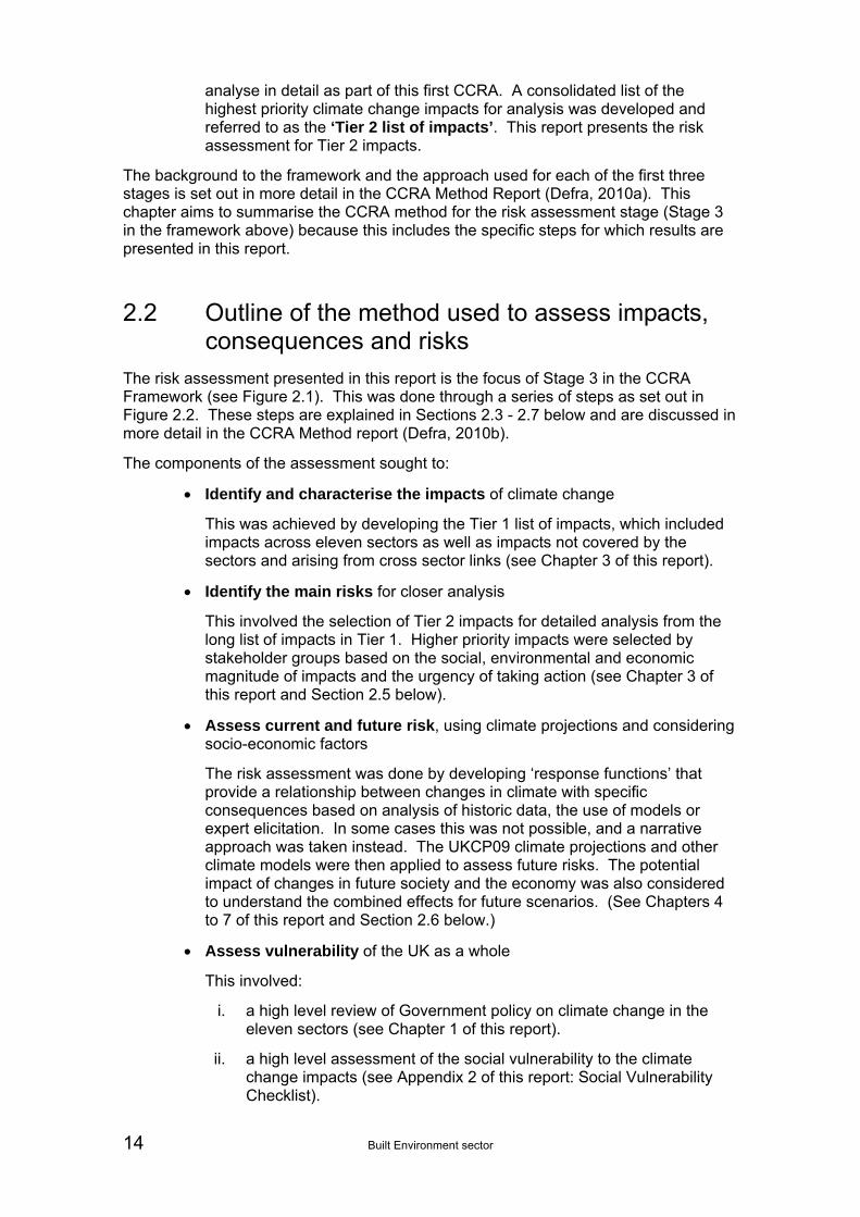
14 Built Environment sector
analyse in detail as part of this first CCRA. A consolidated list of the highest priority climate change impacts for analysis was developed and referred to as the ‘Tier 2 list of impacts’. This report presents the risk assessment for Tier 2 impacts.
The background to the framework and the approach used for each of the first three stages is set out in more detail in the CCRA Method Report (Defra, 2010a). This chapter aims to summarise the CCRA method for the risk assessment stage (Stage 3 in the framework above) because this includes the specific steps for which results are presented in this report.
2.2 Outline of the method used to assess impacts, consequences and risks
The risk assessment presented in this report is the focus of Stage 3 in the CCRA Framework (see Figure 2.1). This was done through a series of steps as set out in Figure 2.2. These steps are explained in Sections 2.3 - 2.7 below and are discussed in more detail in the CCRA Method report (Defra, 2010b).
The components of the assessment sought to:
Identify and characterise the impacts of climate change
This was achieved by developing the Tier 1 list of impacts, which included impacts across eleven sectors as well as impacts not covered by the sectors and arising from cross sector links (see Chapter 3 of this report).
Identify the main risks for closer analysis
This involved the selection of Tier 2 impacts for detailed analysis from the long list of impacts in Tier 1. Higher priority impacts were selected by stakeholder groups based on the social, environmental and economic magnitude of impacts and the urgency of taking action (see Chapter 3 of this report and Section 2.5 below).
Assess current and future risk, using climate projections and considering socio-economic factors
The risk assessment was done by developing ‘response functions’ that provide a relationship between changes in climate with specific consequences based on analysis of historic data, the use of models or expert elicitation. In some cases this was not possible, and a narrative approach was taken instead. The UKCP09 climate projections and other climate models were then applied to assess future risks. The potential impact of changes in future society and the economy was also considered to understand the combined effects for future scenarios. (See Chapters 4 to 7 of this report and Section 2.6 below.)
Assess vulnerability of the UK as a whole
This involved:
i. a high level review of Government policy on climate change in the eleven sectors (see Chapter 1 of this report).
ii. a high level assessment of the social vulnerability to the climate change impacts (see Appendix 2 of this report: Social Vulnerability Checklist).

Built Environment sector 15
iii. Defra is undertaking an assessment of the adaptive capacity of the sectors and will report on this later in 2012.
Report on risks to inform action
This report presents the results of the risk assessment for the Built Environment sector. The results for the other ten sectors are presented in similar reports and the CCRA Evidence Report (CCRA, 2012) draws together the main findings from the whole project, including consideration of cross-linkages, and outlines the risks to the UK as a whole.
Figure 2.2 Steps of the CCRA Method (that cover Stage 3 of the CCRA Framework: Assess risks)

16 Built Environment sector
2.3 Identify and characterise the impacts
Step 1 – Literature review and Tier 1 analysis
This step scoped the potential impacts of climate change on the UK based on existing evidence and collating the findings from literature reviews, stakeholder participation through workshops, correspondence with wider stakeholders and soliciting expert opinion. This work developed the Tier 1 list of impacts (see Appendix 1). The Tier 1 impacts have not been analysed in detail; high level discussion of these impacts is provided in Chapter 3 of this report.
Step 2 – Cross sectoral and indirect impacts
The Tier 1 lists for the eleven sectors in CCRA were compared and developed further to include cross-sectoral and indirect impacts. This was done by ‘Systematic Mapping’, which sets out a flow chart to link causes and effects in a logical process. The impacts that were identified in this step were added to the Tier 1 list of impacts.
2.4 Assess vulnerability
Step 3 – Review of Policy
Government policy on climate change develops and changes rapidly to keep pace with emerging science and understanding of how to respond through mitigation and adaptation. This report includes an overview of selected relevant policy in Chapter 1 as this provides important context for understanding how risks that are influenced by climate relate to existing policies. This information will be expanded in the Economics of Climate Resilience project and the National Adaptation Programme.
Step 4 – Social Vulnerability
The vulnerability of different groups in society to the climate change risks for each sector was considered at a high level through a check list. The completed check list for the Built Environment sector is provided in Appendix 2. This information is provided for context; it is not a detailed assessment of social vulnerability to specific risks. Note that this step is different from Step 10, which considers how future changes in society may affect the risks.
Step 5 – Adaptive Capacity
The adaptive capacity of a sector is the ability of the sector as a whole, including the organisations involved in working in the sector, to devise and implement effective adaptation strategies in response to information about potential future climate impacts. An assessment of the adaptive capacity of the Built Environment sector is ongoing but an initial review based on literature review and stakeholder consultation is presented in Chapter 8. This information is provided for context.
2.5 Identify the main risks
Step 6 – Selection of Tier 2 impacts
The Tier 1 list of impacts for each sector that resulted from Step 2 (see above) was consolidated to select the higher priority impacts for analysis in Tier 2. Firstly, similar or overlapping impacts were grouped where possible in a simple cluster analysis,

Built Environment sector 17
which is provided in Chapter 3. Secondly, the Tier 2 impacts were selected using a simple multi-criteria assessment based on the following criteria:
the social, economic and environmental magnitude of impacts
overall confidence in the available evidence
the urgency with which adaptation decisions need to be taken.
Each of these criteria were allocated a score of 1 (low), 2 (medium) or 3 (high) and the impacts with highest scores over all criteria were selected for Tier 2 analysis. The scoring for each sector was carried out based on expert judgement and feedback from expert consultation workshops (or telephone interviews). Checks were carried out to ensure that a consistent approach was taken across all the sectors. The results of the scoring process are provided in Appendix 3.
Step 7 – Identifying risk metrics
For each impact in the Tier 2 list, one or more risk metrics were identified. Risk metrics provide a measure of the consequences of climate change, related to specific climate variables or biophysical impacts. For example, in the Built Environment sector report, one of the impacts identified is ‘subsidence’ due to increased temperatures and seasonal changes in rainfall patterns. The risk metric identified to measure the consequences of this impact is the number of domestic subsidence claims versus change in summer rainfall. The risk metrics were developed to provide a spread of information about economic, environmental and social consequences. The metrics have been referenced using the sector acronym and a number; the Built Environment sector metrics are referenced as BE1 to BE9.
2.6 Assess current and future risk
Step 8 – Response functions
This step established how each risk metric varied with one or more climate variables using available data or previous modelling work. This step was only possible where evidence existed to relate metrics to specific climate drivers, and has not been possible for all of the tier 2 impacts. This step was carried out by developing a ‘response function’, which is a relationship to show how the risk metric varies with change in climate variables. Some of the response functions were qualitative, based on expert elicitation, whereas others were quantitative.
Step 9 – Estimates of changes in selected climate change scenarios
The response functions were used to assess the magnitude of consequences the UK could face due to climate change by making use of the UKCP09 climate projections. This step used the response functions to provide estimates of future risk under three different emissions scenarios (high carbon emissions, A1FI; medium emissions, A1B; low emissions, B1; see http://ukclimateprojections.defra.gov.uk/content/view/1367/687/ for further details) and for three probability levels (10, 50 and 90 percent, see http://ukclimateprojections.defra.gov.uk/content/view/1277/500/ for further details).
All of the changes given in the UKCP09 projections are from a 1961-1990 baseline.
The purpose of this step is to provide the estimates for the level of future risk (threat or opportunity), as measured by each risk metric.

18 Built Environment sector
Step 10 – Socio-economic change
It is recognised that many of the risk metrics in CCRA are influenced by a wide range of drivers, not just by climate change. The way in which the social and economic future of the UK develops will influence the risk metrics. Growth in population is one of the major drivers in influencing risk metrics and may result in much larger changes than if the present day population is assumed. For some of the sectors where this driver is particularly important, future projections for change in population have been considered to adjust the magnitude of the predicted risks derived in Step 9.
For all of the sectors, a broad consideration has been made of how different changes in our society and economy may influence future risks and opportunities. The dimensions of socio-economic change that were considered are:
Population needs/demands (high/low)
Global stability (high/low)
Distribution of wealth (even/uneven)
Consumer driven values and wealth (sustainable/unsustainable).
The full details of these dimensions and the assessment of the influence they have on the Built Environment sector is provided in Chapter 6. Note that this step is different from Step 4, which considers how the risks may affect society; whereas this step considers how changes in society may affect the risks.
Step 11 – Economic impacts
Based on standard investment appraisal approaches (HM Treasury, 2003) and existing evidence, some of the risks were expressed as monetary values. This provides a broad estimate of the costs associated with the risks and is presented in Chapter 7 of this report. A more detailed analysis of the costs of climate change will be carried out in a study on the Economics of Climate Resilience11.
2.7 Report on risks
Step 12 – Report outputs
The main report outputs from the work carried out for the CCRA are:
The eleven sector reports (this is the sector report for the Built Environment sector), which present the overview of impacts developed from Tier 1 and the detailed risk analysis carried out in Tier 2.
The Evidence Report, which draws together the main findings from all the sectors into a smaller number of overarching themes.
Reports for the Devolved Administrations for Scotland, Wales and Northern Ireland to provide conclusions that are relevant to their respective countries.
11 http://www.defra.gov.uk/environment/climate/government/
Built Environment sector 19
3 Impacts and Risk Metrics Scoping of Impacts
3.1 Identification of Tier 1 impacts and consequences
A wide range of impacts and consequences were identified for the Built Environment sector as a whole based on the sector scoping report (Capon, 2010), the CCRA scoping study (Watkiss et al., 2009) and consultation with sector specialists. This is referred to as the ‘Tier 1’ list of impacts.
Consultation was undertaken with a range of organisations in the preparation of the sector scoping report including representatives of national and regional government, research and consultancy organisations, the National Trust and the ABI.
Subsequent analysis involved a review of current research literature as well as further discussions with a number of individuals and organisations. This has included representatives from DCLG, Defra, CABE and the Met Office.
There was also a Built Environment sector workshop held 28th May 2010, which was attended by 23 people drawn from across the sector. The participants reviewed the list of sector impacts identified in the ‘Tier 1’ risk assessment and made additions/ amendments as necessary. Names of attendees are included in the Acknowledgements section12.
While many potentially adverse impacts and consequences were identified, there are also a number of opportunities. A total of 48 impacts and consequences for the Built Environment sector were identified during this scoping process. These are listed in the Tier 1 list in Appendix 1. These were clustered into 5 main overlapping areas or themes (Figure 3.1), namely:
Construction
Cultural Heritage
Homes
Places of Work
Spatial Planning.
Impacts and consequences are grouped with others that they are strongly linked to and placed with biophysical impacts on the left and the more socio-economic consequences for the sector on the right. The interactions between impacts and consequences are explored in more detail in the systematic mapping (Step 2 of the CCRA method). The numbers in brackets refer to the individual impact number in the Tier 1 list.
12 The following web-link provides access, upon registering, to the Built Environment Sector workshop record: http://ccra.defra.gov.uk

20 Built Environment sector
Figure 3.1 Impact clusters for the Built Environment sector
3.2 Scoring of Tier 1 impacts and selection of Tier 2 consequences
There are over 700 impacts identified in the Tier 1 assessment for all eleven sectors and more than forty in the Built Environment sector (including omissions identified during or subsequent to the workshop). With the time and resources available for the CCRA, it simply would not have been possible to undertake a detailed analysis of all of the Tier 1 risks, and so a selection process was carried out.
The CCRA pilot study involved work with Defra experts and consultation with the CCRA Forum and Project Steering Group on a simple selection process to identify impacts for further assessment in the Tier 2 risk assessment. The criteria agreed by the technical advisory group to the CCRA (the In House Experts Group) to be used to prioritise the consequences were:
Magnitude of consequences
- Economic
- Social
- Environmental
Likelihood of the consequence occurring
Urgency with which a decision needs to be made.

Built Environment sector 21
The criteria were equally weighted and the scores were derived according to the narratives in Tables 5.1 to 5.3 of the methodology report (Defra, 2010b).
The scoring is primarily based on qualitative information and attempts to record ‘orders of magnitude’ rather than offering precision at this early stage of the study. The scoring is similar to the Cabinet Office’s National Risk Assessment, although at a higher level, given the wide ranging uncertainties in climate change impacts assessment, and with an equal emphasis on environmental impacts.
The built environment impacts were scored according to the guidelines above using the following formula:
3
Urgency
3
Likelihood
9
EconomictalEnvironmenSocial*100
Different scoring methods were considered but application of more complex approaches would indicate an overly high level of precision in the evidence and in most cases would lead to bias in the selection of impacts towards particular criteria. For example a logarithmic scale (1, 10, 100,..) could be used for the magnitude of impacts but this would lead to only high magnitude impacts being selected and make urgency and likelihood scores irrelevant.
From a risk perspective considering logical rules related to risk AND urgency is more appropriate but analytically this makes little difference in terms of what risks are selected for Tier 2.
The scores are included in Appendix 3. These scores were also informed by consideration of social vulnerability (see Appendix 3). The overall outcomes of the scoring are shown in Table 3.1 with Table 3.1(a) showing the impacts which scored above the threshold for inclusion in Tier 2 and Table 3.1(b) showing how the same impacts relate to levels of urgency and risk.
Table 3.1(a) Outcomes of the scoring
Selected (threshold >30) Marginal (threshold = 20) Excluded (below score of 20)
Urban Heat Islands (25,39)
Water Availability (13,14)
Overheating of Buildings (24)
Flood Damage (1,2,3,4,10,21,22,23)
Demand for Water (27)
Effectiveness of Green Spaces (20,46)
Damage from Heat/Drying (28,30)
Pest Infestations (31,34,44)
Demand for Heating (26)
Soil Drying, Heave & Subsidence (15,40)
Seasonal Interruptions (36, 38)
Biodiversity/species balance (29, 41)
Rainwater Penetration (7,8)
Condensation, Damp, Mould, etc. (17,44)
Soil Erosion (5) & Landslips (6)
Waste Management (34,37)
Fires (43)
Water Availability for construction (16)
Sulphates in Soils (45)
Dust Generation (48)
Cold Weather Damage (32,33)
Urban Creep (18)
Use of Outdoor Spaces (35)
Water Logging (47)
Damage from Tree Roots (19,42)
Wind Damage (9,11,12)

22 Built Environment sector
Table 3.1(b) Alternative scoring rule based on risk AND urgency
Hig
h
Fires (43)
Water availability for construction (16)
Use of Outdoor Spaces (35)
Flood Damage (1, 2, 3, 4, 10, 21, 22, 23)
Demand for Water (27)
Effectiveness of green spaces (20, 46)
Damage from heat/drying (28, 30)
Pest infestations (31, 34, 44)
Demand for Heating (26)
Soil Drying, Heave & Subsidence (15, 40)
Waste Management (34, 37)
Biodiversity/Species balance (29, 41)
Seasonal Interruptions (36, 38)
Urban Heat Islands (25, 39)
Water Availability (13, 14)
Overheating of Buildings (24) M
ediu
m
Dust generation (48)
Sulphates in soils (45)
Water Logging (47)
Cold weather damage (32, 33)
Damage from tree roots (19, 42)
Wind Damage (9, 11, 12)
Rainwater penetration (7, 8)
Condensation, Damp, Mould etc. (17,44)
Soil Erosion (5) & Landslips (6)
Ris
k (q
ual
itat
ive
esti
mat
e)
Lo
w
Urban Creep (18)
Low Medium High
Urgency of decisions
3.3 Selected Tier 2 risks
On the basis of the scoring undertaken and the comments made during the sector workshop, the following Tier 2 impacts were selected for analysis:
Urban Heat Island – Consideration of the significant uplift in urban temperature in comparison to neighbouring rural locations given projected increases in average temperatures.
Subsidence – Risk of subsidence increased by drying out of vulnerable soil areas.
Overheating of buildings – Risk of overheating in buildings including homes and within the working environment, arising due to inadequate design or lack of cooling capacity in a local environment.

Built Environment sector 23
Effectiveness of green space – Risk of exacerbation of urban heat island effects arising from the reduction in the capacity of urban green space to provide cooling.
Demand for heating (opportunity) – Warmer winters potentially reduce demand for space heating with consequences for both household demand and new build design.
While the first four of these are risks to the Built Environment sector, the fifth impact, reduced demand for heating, is taken forward as a positive benefit arising from climate change, in accordance with the CCRA methodology.
In addition, the following significant built environment impacts exceeded the threshold for inclusion in Tier 2 and are included in this report, although they were analysed within other sectors of the CCRA:
Water availability and demand for water, from the Water sector analysis (Rance et al., 2012).
Flood damage, from the Floods and Coastal Erosion sector analysis (Ramsbottom et al., 2012).
3.4 Discussion of other risks
Further consideration is given in this section to some of the risks that are not covered by the analysis including (a) risks with scores in the marginal category, (b) risks in the high score category but where no data were available for analysis and (c) risks specifically requested to be covered by consultees. These risks were:
Damage from Heat/Drying (28, 30), which had a high score but limited data.
Pest Infestations (31, 34, 44), which had a high score but limited data. Specific issues were raised in terms of the increase in levels of moulds and pest infestations resulting from milder, wetter winters. This was identified as an issue for cultural heritage buildings in particular, with little additional evidence available in the case of wider domestic or non-domestic properties. Given the limited availability of robust evidence linking changing climate with specific pests or mould growth this was not taken forward for further analysis.
Seasonal Interruptions in the Construction Industry (36, 38), which had a marginal score.
Rainwater Penetration (7, 8), which had a marginal score.
Condensation, Damp and Mould (17, 44), which had a marginal score.
Indoor Air Quality, which was raised as a specific issue by consultees.
The built historic environment, which was raised as a specific issue by consultees.

24 Built Environment sector
3.4.1 Seasonal interruptions in the construction industry
Although the market share of off-site construction is increasing13, most construction processes are still carried out on-site and are therefore vulnerable to extreme weather, which can slow or stop progress (Graves & Phillipson 2000). Health and safety considerations can also lead to suspension of some construction activity under certain climatic conditions. The consequences of such disruption are increased construction times and late delivery of finished buildings. Weather-damage may also cause excess wastage of construction materials. In his recent report for the Technology Strategy Board, Gething (2010) identified several issues, all of which need to be considered on a short-term time-scale, i.e. within the next 10 years.
Hotter, drier summers will lead to temperature limitations for some building processes, e.g. laying concrete. Working conditions will also be affected; site accommodation huts currently in use are likely to become intolerable in future summers, as are internal conditions in incomplete/unserviced buildings. Water-intensive construction processes will also be affected by reduced summer rainfall and more frequent summer droughts.
Stability during construction could also be vulnerable to climate change impacts such as hotter drier summers, warmer wetter winters and more frequent extreme weather events. An increase in inclement winter weather, e.g. more extreme rain, could result in more working days being lost on-site. On the other hand, a reduction in the number of frosts will increase the number of days available to use concrete and cements, for example.
3.4.2 Rainwater penetration
Rain penetration occurs most frequently through walls exposed to the prevailing wet winds, which are usually south-westerly or southerly (Trotman et al., 2004). The risk of wind-driven rain and rainwater penetration of buildings in the current climate is assessed using a wind-driven rain index derived by BRE (British Standards Institution 1992). As would be expected, the areas at greatest risk include Scotland (The Scottish Government 2009), parts of Cumbria, the west of Wales and Southwest England. Historically, local design in Scotland has taken this risk into account through detailing, such as recessed window and door reveals, and render finishes (Gething, 2010).
The UKCP09 projections show an increase in mean winter precipitation but not in mean winter wind speed. Thus wind-driven rain may increase under climate change. This could raise the severity of expected rain penetration (e.g. from moderate to severe) to a level where a building’s external elements, materials or joints, no longer provide the precipitation resistance needed. This increased affect of wind driven rain will be particularly relevant where external walls do not have a suitable cavity or rain screen (The Scottish Government, 2009). For example, driving rain will affect properties with rendered walls to a greater extent than those with cladding. Cavity wall insulation - which is often recommended to increase the thermal efficiency of buildings - may actually render buildings more vulnerable to rain penetration in conditions of driving rain (Stirling, 2002 and Austin et al., 2008).
13 The off site construction of buildings, building elements and structures is currently worth around £2-3 Billion per year and accounts for around 2% of the total construction market – a market share increasing by 25% per year (Offsite Production in the UK Construction Industry – prepared by HSE and published by Buildoffsite, June 2009 www.buildoffsite.com).

Built Environment sector 25
3.4.3 Condensation, damp, mould
Dampness within a building is most commonly caused by condensation, rain penetration (see above) or rising damp and can lead to a variety of problems with the building fabric; blistering paint, bulging plaster, timber rot, reduced effectiveness of thermal insulation, sulphate attack on brickwork and corrosion of metal elements leading to brickwork cracking. The risk of condensation is greatest in areas which are colder, moister and/or poorly ventilated. Mould growth is likely where surfaces or air are continuously or frequently damp (Trotman et al., 2004). Mould can have significant consequences for human health, most commonly allergic reactions to the spores, especially asthma. However other health effects associated with toxic and psychological reactions and fungal infections have been noted (Sanders et al., 2004).
The main climate driver for condensation, damp and mould is increased winter precipitation and consequent higher humidity levels. More research is needed to determine whether the risks of mould growth are greater in highly energy-efficient buildings, which have increased insulation but reduced air infiltration (Crump et al., 2009).
3.4.4 Damage from heat/drying
The performance of building materials may be affected by climate change impacts such as higher temperatures and increased UV radiation levels (Gething, 2010). This may cause greater thermal expansion and movement in metallic building components such as cladding. The rate of corrosion reactions may also increase, although this is likely to be a relatively small change. Plastics, e.g. uPVC windows, doors, gutters, weatherboards and downpipes, are expected to degrade more quickly under climate change, but the extent of such decay has yet to be quantified. There is also an increased risk of failure for poor quality glazing, e.g. due to thermal shock (Graves and Phillipson, 2000).
3.4.5 Pest infestations
Some types of pest, house dust mites and cockroaches for example, cause a risk to health. Due to the buffering effects of the carpets and soft-furnishings in which mites live, it is unlikely that climate change will have any effect of the level of mites in UK properties. The spread of cockroaches between buildings is dependent upon the external environment. With a progression to warmer summers there is an increased likelihood of infestations occurring in properties unconnected to the source (Sanders et al., 2004).
Timber structures, both modern and historic, can also be damaged by infestations of pests such as wood-boring beetles (e.g. house longhorn beetle) and termites. The risk of existing colonies of pests spreading may increase as temperatures rise. Changes in humidity will also impact the breeding cycle (Graves and Phillipson, 2000). A significant risk is through the importation of infested timber, particularly if future climate conditions are more favourable to imported species.
3.4.6 Indoor air quality
People spend approximately 90% of their lives indoors on average. Therefore, indoor air quality is a fundamental determinant of the health, comfort and performance of people in buildings. It depends, however, on a combination of factors, any of which

26 Built Environment sector
can cause discomfort and/or health problems for occupants. In addition to condensation, damp and mould and pests, which have already been discussed, a key issue is the presence of pollutants in indoor air. Volatile Organic Compounds (VOCs) and formaldehyde may be generated internally from natural metabolic processes, household consumables (particularly cleaning products), the building fabric (particularly adhesives, solvents and treatments), furniture and finishes (for example carpets, paints, etc) (Sanders et al., 2004). Activities such as cooking, heating and smoking may generate other pollutants, such as nitrous oxides and particulates (Crump et al., 2009). Externally generated pollutants and ground contaminants, such as radon gas, may also enter buildings through windows or other means of ventilation (Sanders et al., 2004).
This is particularly an area of concern for new energy-efficient buildings, which are constructed to have much greater air-tightness than traditional stock (Davis and Harvey, 2008). The resulting lack of air infiltration could potentially lead to build-up of pollutants, high humidity and condensation (leading to mould growth), damage to structures and proliferation of house dust mites (Crump et al., 2009). In the housing sector, for example, Crump et al concluded that there is an urgent need for research into the performance of highly energy efficient homes with respect to the quality of the internal environment ventilation systems used, and the impact on the health and wellbeing of occupants.
3.4.7 The built historic environment
Many of the climate change impacts and consequences affecting the built historic environment are the same as elsewhere in the Built Environment sector. Nevertheless, the built historic environment is unique in terms of its non-renewable character and the potential for damage and loss. Many historic buildings, sites and landscapes have already experienced and survived significant climatic changes in the past and may demonstrate considerable resilience in the face of future climate change. However, many more historic assets are potentially at risk from the direct impacts of future climate change (English Heritage, 2008). These include the following.
Rising sea levels and a possible increase in storminess endangers historic landscapes, structures, buildings and archaeology in the coastal zone, for example, the Heart of Neolithic Orkney World Heritage Site including Skara Brae in Scotland (Scottish Government, 2009).
Increased extremes of wetting and drying heighten the risk of ground subsidence and accelerated decay of stonework.
More frequent intense rainfall can cause increased erosion of archaeological sites and also overload roofing and gutters, penetrate traditional materials (e.g. thatch, cob, wattle-and-daub, etc) or deliver pollutants to building surfaces, while flooding brings catastrophic loss (Sabbioni et al., 2008), making historic buildings difficult to insure.
Changes in humidity affect the growth of microorganisms on stone and wood, and the formation of salts that degrade surfaces and influence corrosion, as well as increasing mould outbreaks within buildings.
Changes in the distribution of pests (see above) threaten the integrity of historic buildings, collections and designed landscapes.
Freeze/thaw events can cause fractured stonework and burst pipes, rainwater goods and radiators (National Trust).

Built Environment sector 27
Historic thatched properties are at greater risk of fire damage (which may or may not be linked to climate change).
Subsidence is a greater risk for some historic buildings.
Work ongoing in this area includes the interdisciplinary PARNASSUS programme and other projects under the Science and Heritage Programme, funded by the Arts & Humanities Research Council and Engineering and Physical Sciences Research Council.
3.5 Cross-sectoral and indirect consequences
Many of the risks examined for this sector are linked or interact with risks in other sectors. This section (i) explores the cross-sectoral links in more detail based on the systematic mapping of causes, processes and consequences; and (ii) identifies the risks in other sector reports that are pertinent to the sector.
3.5.1 Systematic mapping
For the Built Environment sector, most of the cross-sectoral links were already identified in the Tier 1 report, although the systematic mapping has emphasised them.
Heat-related issues such as the Urban Heat Island, overheating and the effectiveness of green space particularly affect health and energy demand. There is an association between green space and better mental and physical health.
Indoor air quality also affects health.
Water resources and quality are related to water availability and management issues for the built environment.
Transport is necessary for sustaining the urban system. Climate impacts such as flooding and subsidence can affect transport as much as the built environment. Transport failure modifies use of the Built Environment sector and reduces business productivity.
Tourism can be negatively impacted by extreme weather events, which damage the built environment, e.g. 2004 Boscastle flood.
Hotter drier summers may have a positive impact upon tourism.
Heritage and tourism are closely interrelated.
Biodiversity changes, e.g. in population and productivity of species, may have implications for planning and land-use.
3.5.2 Risks addressed in other sector reports
The following cross-sectoral risks are included in the analysis carried out in other sector reports:
Water availability and demand for water (Water sector)
Flood damage to properties (Floods and Coastal Erosion sector)

28 Built Environment sector
Heat-related mortality and morbidity – both in summer and winter (Health sector)
Flood impacts on mortgages (Business sector)
Loss of staff hours due to high building temperatures (Business sector)
Energy demand (Energy sector)
Wildfires (Biodiversity & Ecosystem Services sector)
Transport infrastructure (Transport sector).
In addition, cultural heritage is included to a limited degree in the consequences for tourism assets (Business sector).
The wildfire and transport infrastructure risks are discussed at an overview level below. The analysis for the other risks in this list is covered in more detail in Chapters 4 to 7 of this report. The content has been taken from the other sector reports and these should be referred to for full context of the analysis of these risks.
Wildfires – Increased risk of wildfire (Risk metric BD12)
An increased prevalence of hotter, drier conditions implies a greater risk of fire. Some ecosystems, such as woodlands, semi-natural grasslands, heathlands, and those on peat soils (e.g. bogs) are particularly sensitive to fire. Wildfires can also impact upon other sectors, including human health, forestry, agriculture, and the built environment and cause disruption to business activities and transport (McMorrow et al., 2005). Where wildfire prone sites (gorse, heath, grass) are located in close proximity to highly populated areas and transport infrastructure both the frequency and impact of even relatively small wildfires can be significant (South East of England Regional Wildfire Group and Home Counties Operational Wildfire Group, April 2010).
Analysis of recent data held by the Department for Communities and Local Government (DCLG) shows a strong correlation between the frequency of fire and the ‘heatwave’ years of 1995, 2003 and 2006 (Gazzard, 2010). Within the biodiversity sector analysis, the 11-member Regional Climate Model (HadRM3) ensemble associated with UKCP09 has been used and model results (% difference) extracted for national parks across England, Scotland and Wales. These show a 30-50% increase in the McArthur Forest Fire Danger Index between the 1980s and the 2080s (ensemble mean; medium emissions scenario), with the largest changes in the south. For Northern Ireland, the change in risk is lower at 10-30% (CCRA, 2012a). Note that these figures relate to annual average change only; they give no indication of the possible impact of changing interannual variability or extreme events such as heat waves.
Transport Infrastructure
Transport is necessary for sustaining the urban system. Climate impacts such as flooding and subsidence can affect transport as much as the built environment. Transport failure affects the use of the built environment and reduces business productivity, particularly failure due to flooding and inundation and failure due to land movements, i.e. subsidence and landslides. These impacts were analysed within the Transport sector.
Flood disruption/delay to road traffic (Risk metric TR1): Within the context of the CCRA, analysis focused on one aspect of flooding and inundation disruption, namely the delay
Built Environment sector 29
to road traffic. The widespread flooding of major and minor roads in 2007 gives a very useful guide to the scale and costs of the risks involved. It has been estimated that the cost of disruption was of the order of £100m and the probability of this type of event is likely to increase with climate change. The assessment suggests that the economic cost of disruption from floods is projected to remain relatively low to the 2050s with the potential to increase to an event similar to 2007 on an almost annual basis by the 2080s.
Landslide impacting on the road network (Risk metric TR2): With respect to land movement of roads, the analysis within the Transport sector focused predominantly on landslip/landslide. In general, subsidence is effectively managed through existing road maintenance programmes and thus is not considered to be a significant issue. The length of roads currently under some kind of threat from landslides in the UK runs into thousands of kilometres. However, the length of road at risk is projected to remain similar to current levels over the next 40 years, with some increase in risk beyond this period.
For both the above metrics, there is still uncertainty within the qualitative analysis. Hence they should be considered solely as indicative of the risk.
3.6 Selection of risk metrics
Risk metrics provide a measure of the consequences of climate change. For national risk assessment, ‘good’ metrics should satisfy a number of criteria, i.e. they should:
Be sensitive to climate but also allow the disaggregation of climate and socio-economic effects.
Provide a measure of changing probability or consequences relevant to a baseline, so historical data are required to establish the current situation.
Be presented at the national and regional scales, based on high quality data that are collected and held by Government departments, agencies or research institutes. The use of Government data should provide consistency between sectors and allow the metrics to be repeatable in subsequent CCRA cycles.
Reflect economic, environmental and social consequences of climate change; some metrics may be monetised but others may simply indicate the areas affected or consequences for vulnerable groups of society.
Be relevant/have legitimacy to the relevant Government policy.
For the Built Environment sector the identification of metrics for direct biophysical impacts, such as flood risk to property, is a relatively straightforward task but these on their own are insufficient to express risk in this sector as they do not provide enough information to measure the economic, social and environmental consequences of climate change. Within the sector it is often the consequences for users of the built environment which are more relevant; for example, the effect overheating in buildings may have on a workforce or the number of homes at increasing risk of flood and the consequences this may have for their residents.
The selected metrics for the Built Environment sector are listed below together with relevant metrics from other sectors where the analysis is included in this report.

30 Built Environment sector
3.6.1 Built Environment risk metrics
Risk metrics for the five key impacts taken forward in the Built Environment sector analysis are:
BE1 – Increase in temperature caused by the Urban Heat Island effect. This describes the increased temperature within urban areas compared to their rural surroundings. During the heat wave events across South East England in August 2003 and July 2006 night-time air temperatures in London were 6–9°C higher than those recorded for rural locations south of London (Mayor of London, 2006). Such effects have been observed in urban centres elsewhere in the UK e.g. Birmingham and Manchester. The August 2003 heatwave led to 2,139 excess deaths in England and Wales, the majority of which were in the London area.
BE2 – Number of household incidents of subsidence. The gradual increase in average temperatures and seasonal changes in rainfall patterns may lead to changes in the cycle of wetting and drying of soils thereby increasing the soil moisture deficit. Drier soils increase the risk of subsidence on susceptible soils; as a result the foundations and structures of older buildings will be damaged. Subsidence is currently the second most important hazard to property insurers in the UK. Insurance claims for the period 2002 to 2009 exceeded £1.8 billion, an average of over £200 million per year. Costs during the very dry year of 2003 were about £400 million.
BE3 – Number of days that threshold temperatures are exceeded (in relation to overheating of buildings). As temperatures rise, summer internal comfort is becoming more important in both domestic and commercial buildings due to potential consequences for health and productivity. Particularly in commercial space, this has major implications for building design in terms of maladaptation and reliance on air conditioning and general working conditions and associated productivity.
BE5 – Change in the effective area of urban green space. Green infrastructure has been shown to have a beneficial cooling effect in urban areas. During prolonged hot and dry periods, grass and other vegetation can dry out, severely reducing the cooling capacity of such areas. Green infrastructure also contributes to better mental and physical health.
BE9 – Demand for heating. Warmer winters lead to reduced demand for energy for heating and thus reduced energy bills. This is also a design opportunity for new build, as reduced heating capacity/plant would be required.
3.6.2 Water availability risk metrics
The following risk metrics relevant to the Built Environment sector were analysed within the Water sector report.
WA5 – Supply-demand deficits (Dry Year Annual Average design condition) (Ml/d or %). The supply-demand balance is calculated based on the water available from surface water and groundwater sources and the demand for water. Water companies estimate the amount of water available for abstraction based on hydrological or hydrogeological conditions, licence conditions and works capacities. These calculations are combined with 25 year demand forecasts to estimate when resources

Built Environment sector 31
zones will fall into deficit, requiring investment in demand or supply side measures.
WA6 – Population affected by a water supply-demand deficit (No. or %). The population affected by a supply-demand deficit (when water resource zones fall into deficit and require demand or supply-side measures) is calculated at the same time as WA5.
Metrics WA5 and WA6 are quantitative.
3.6.3 Flooding risk metrics
The following risk metrics relevant to the Built Environment sector were analysed within the Floods and Coastal Erosion sector report.
Residential properties
FL6a Residential properties at significant likelihood of flooding14 and FL6b Expected Annual Damages to residential property (EAD)
Commercial properties
FL7a Non-residential properties at significant likelihood of flooding and FL7b Expected Annual Damages to commercial property (EAD)
Insurance of residential properties
FL13 Residential properties at significant likelihood of flooding (to assess insurance impacts). In England, the Government and the ABI have agreed a statement of principles in relationship to the continued provision of insurance against flood risk for most households. In this agreement, significant likelihood of flooding (i.e. 1:75 years or more frequent) is identified as the threshold that insurers use to consider their approach to the provision of insurance cover.
Limitations
The metrics are defined by type of flood (tidal/coastal, river and surface water) because this is the way in which the data are presented in the studies used to provide information for calculating the metrics. There are some important limitations to the analysis:
Metrics have been calculated for river and tidal flooding, but not for surface water flooding. Whilst estimates are available of the number of properties currently at risk for surface water flooding, there is a lack of suitable information of potential future risks.
The calculations do not include Scotland and Northern Ireland (about 6% of overall flood risk) because of a lack of suitable information.
3.6.4 Health risk metrics
The following risk metrics relevant to the Built Environment sector were analysed within the Health sector report.
14 Defined as the 1.3% annual probability of flooding (or once in 75 years on average).
32 Built Environment sector
HE1 – Temperature Mortality (Heat) and HE5 Temperature Mortality (Cold)
HE2 – Temperature Morbidity (Heat) and HE6 Temperature Morbidity (Cold)
HE3 – Flood related deaths
3.6.5 Business risk metrics
The following risk metrics relevant to the Built Environment sector were analysed within the Business sector report.
BU6 – Increased exposure for mortgage lenders
BU10 – Loss of staff hours due to high internal building temperatures
3.6.6 Energy risk metrics
The following risk metrics relevant to the Built Environment sector were analysed within the Energy sector report.
EN2 – Energy demand for cooling

Built Environment sector 33
4 Response Functions
4.1 Introduction
The purpose of this step is to understand the sensitivity (according to the available evidence) of the selected metrics to changing climate conditions. It was based on review and synthesis of existing research outputs and government analyses and included recording key assumptions and uncertainties related to the assessment.
Given the varied and extensive form within the built environment, and a complex interplay with spatial planning, water and energy resources (among others) it is difficult to succinctly capture the direct impacts of changing climate as exemplified in the UKCP09 climate projections. Instead, the selected metrics were developed as a means of capturing key issues, as identified via the process outlined in Section 3, and enabling risk assessment, as described in Chapter 5.
For each metric, suitable datasets were sought from publicly available sources (either government analyses or wider published research); this will provide the basis for consistency in the delivery of future risk assessments. Suitability in this case meant not only data that was scalable with a given climate parameter, but that also enabled consideration of the wider economic (where practicable, via monetisation), environmental and social consequences.
This section describes the sensitivity of selected metrics to the UKCP09 future climate projections, particularly warmer conditions with drier summers. The metrics discussed here consider both domestic and non-domestic buildings.
While cultural heritage sites were explicitly considered in both the scoring of impacts and the selection of these metrics, some of the issues highlighted during the sector workshop as being of particular note for these sites did not score above the threshold for inclusion in the Tier 2 analysis. It was also noted in the workshop however that many historic buildings face the same risks as more modern buildings, although the consequences of these risks can be very different, often determined by the structure and fabric of each building. For these reasons, risks which are specific to cultural heritage are not included in this analysis. Risks relating to cultural heritage sites are discussed in Section 3.4.7.
Other relevant impacts and consequences have been considered in other CCRA sectors, as discussed in Section 3.5.2.
This section sets out the response functions that were developed for the Built Environment sector, which are denoted by risk metrics BE1, BE2, BE3, BE5 and BE9. The missing number references are metrics that were considered in the scoping of risk metrics but that were not taken forward for analysis.
Following the sub-sections for each of the BE metrics, there are sub-sections on metrics that are covered by other sectors. These are Water metrics (WA5 and WA6), Floods metrics (FL6, FL7 and FL13), Health metrics (HE1, HE5, HE2 and HE3), Business metrics (BU6 and BU10) and Energy metric (EN2). The full details and context for these analyses can be found in the reports for these sectors.

34 Built Environment sector
4.2 BE1 – Urban Heat Island
The Urban Heat Island (UHI) is a phenomenon that has been recognised since the beginning of the 19th Century. Extensive urban development alters the surface energy balance in such a way that the temperature at the centre of a large city can be several degrees higher than in the surrounding rural areas. The effect is more pronounced at night.
A number of factors contribute to the development of this urban microclimate. There is greater absorption and storage of short-wave solar radiation by the urban fabric during the day. This energy is then re-emitted at night as long-wave radiation (although the rate of heat loss is limited by the reduced sky-view factors of urban street canyons). The majority of surface water from rainfall is drained away and is therefore not available for evaporative or evapotranspirative cooling. Anthropogenic heat emissions, such as exhaust air from air-conditioning systems, also act to increase the local air temperature.
Due to uncertainty and lack of available data at the time of the CCRA analysis, a quantitative response function was not developed for this metric.
Understanding the UHI, both in the present-day climate and its future evolution under climate change, is an active and rapidly evolving area of research. The EPSRC has funded a number of research programmes in this area, including LUCID (focussed on London) and SCORCHIO (focussed on Greater Manchester).
In winter the UHI can be beneficial. The LUCID project found that the UHI currently has a significant net energy benefit for London, as it reduces winter heating demand (Mavrogianni 2009). However, in summer, particularly during heat waves, the urban heat island prevents the city from cooling down, maintaining night-time temperatures at a level that affects human health and comfort.
4.2.1 Magnitude of UHI
Urban Heat Islands have been observed in a number of UK cities. For example, in Birmingham, night-time minimum temperatures have been observed to be up to 5°C higher within the city than in surroundings rural areas during periods of high atmospheric stability (Tomlinson, 2010; Unwin, 1980).
Recent work by the SCORCHIO team included the development of a spatial temperature profile across Greater Manchester. The results available to date suggest a maximum UHI intensity (defined as the difference in temperature between urban and rural locations) of around 3°C during the day increasing to around 5°C at night (Smith et al., 2011). The Royal Meteorological Society’s Big Urban Heat Island Experiment campaign is ongoing15, with the aim of mapping the UHI in a number of UK cities and towns. Results from this study in relation to Manchester suggested a maximum difference between the warmest and coolest areas as high as 10.0°C (Knight, 2010).
In London, spatial pattern mapping of the UHI during the summer of 2000, over the hour between 02:00 – 03:00 for a series of calm dry nights, revealed areas with UHI intensity in excess of 6°C. More recent observations have noted extreme UHI intensities in excess of 7°C; in August 2003, for example, the UHI intensity reached a maximum value of 9°C (Mayor of London, 2006).
The UHI intensity is typically greatest in the centre of a city and decreases when moving outwards in a radial direction. However, there are also local variations within
15 http://www.metlink.org/urban

Built Environment sector 35
the city according to the land-use type (Smith et al., 2011). Urban green spaces are generally cooler than the surrounding built-up areas, as illustrated for Regents Park and Richmond–Wimbledon Common in London (Figure 4.1).
4.2.2 Impacts of the UHI
The link between increased summertime temperatures and heat-related mortality has also been investigated by a number of authors. Analysis of single events has provided evidence of a link between UHI effect and heat deaths (Milojevic, 2011). In the case of the summer period of 26 May - 21 June 2006 in London, the percentage of heat-related deaths attributable to the UHI effect was determined as 37.7% in outer London rising to 47.2% in central London; the corresponding mean differences in daily maximum temperature for these zones were +0.3 and +0.5 °C respectively.
The LUCID project has also investigated the contribution of the UHI effect to indoor thermal comfort and summertime overheating. The analysis revealed that the microclimatic characteristics of the specific site and the thermal quality of the individual dwelling were greater indicators of risk than the location of the building within the Urban Heat Island (Mavrogianni et al., 2010).
4.2.3 Anthropogenic heat contribution to the UHI
SCORCHIO examined the anthropogenic heat contribution to the Urban Heat Island in Manchester. In winter it was 39% at night and 75% during the day, whereas in summer the nocturnal and daytime contributions were 17% and 25% respectively.
LUCID found that the UHI currently has a net-energy benefit for London, as it reduces winter heating demand. However in future, the net energy balance will depend critically on levels of uptake of air conditioning (Kolokotroni, 2010). If air-conditioning is widely installed (e.g. domestically) the summer energy demand will rise. Furthermore the UHI effect will be exacerbated by the exhaust heat output.
4.2.4 Summary
The relationship between urban morphology and the UHI effect is complex; modelling of such effects increasingly involves use of a variety of spatial and temporal scales beyond current regional climate change models (Section 5.4.1). Furthermore, the CCRA analysis was undertaken before completion of the LUCID and SCORCHIO projects.
The magnitude of difference between urban and rural temperature is seen to be at its greatest during night-time periods (typically 23:00 – 03:00). The relationship between Urban Heat Island effects and heat-related mortality is an area of ongoing research. A number of studies have shown that prolonged periods of elevated night-time temperatures contribute to heat stress (e.g. Dousset et al., 2011). Thus the change in minimum night-time temperature during summer months can be considered as an important variable in assessing the risk to human comfort and health presented by UHI effects.

36
Figure 4.1 Land Surface Temperature at 21:00 on 12 July 2006
Source: LUCID project (2007 – 2010)

Built Environment sector 37
Given the degree of uncertainty in future evolution of the UHI and the lack of model output data available at the time of analysis, a response function is not defined. Instead a qualitative assessment is made with change in mean average minimum summer temperature being selected as an appropriate climate variable.
Note that the CCRA Health sector assessment has taken a different approach and considered the number of times a specific daily mean temperature threshold measured over time is exceeded. Within this assessment, however, the focus is upon the UHI effect and how temperatures in urban centres may increase. The relative magnitudes of the UKCP09 projected increases in summer minimum temperatures provide a means of assessing the likelihood that present threshold temperatures for action during heat wave events are exceeded more frequently (see Section 5.4).
The analysis carried out for metric BE1 is based on specific large cities in England. Whilst the UHI effect is likely to occur to some degree in all large urban areas in the UK, the magnitude will depend on a range of factors including size and location.
4.3 BE2 – Subsidence
Changes in climate, both increased temperatures and changing rainfall patterns, may lead to greater levels of variability in the wetting and drying of shrink-swell soils. This increases the risk of subsidence and damage, particularly to some building designs with susceptible foundation types and ground floor types. For example, a substantial increase in the drying of such clay soils was observed during the dry summers of 1989 and 1990 (Driscoll and Skinner, 2007) together with a corresponding increase in the number of insurance claims (Graves and Phillipson, 2000).
Subsidence claims for domestic dwellings amounted to £175 million in 2009 with 29,700 notified claims (Source: Association of British Insurers). Figure 4.2 shows the shrink-swell potential of soils throughout the UK. It can be seen that the level of risk is most significant in certain areas of England, with reduced or limited risk in other parts of the UK.
A response function has been developed, which relates the change in average summer rainfall to the projected number of notified claims (as an indicator of actual incidents of subsidence). The response function is developed on a regional basis for the whole of the UK. The baseline number of incidents per region is extrapolated from the national total using the number of dwellings and the percentage area of high-risk soils in each region. For the purposes of this analysis, only areas with significant soil shrink-swell potential (Figure 4.2) are considered.
A linear relationship between subsidence claims and future changes in summer rainfall has been obtained by plotting the total number of claims within each year (within the data supplied by the Association of British Insurers) against the percentage change in summer rainfall (in comparison with the 1961 – 1990 average) for each year as recorded by the Met Office for the years 2002-2009 (Figure 4.3). It should, however, be noted that, although this appears to give a good correlation, the data sample is so small that the relationship must be considered highly uncertain.
This metric primarily applies to England, where the areas of significant shrink-swell potential exists (Figure 4.2).
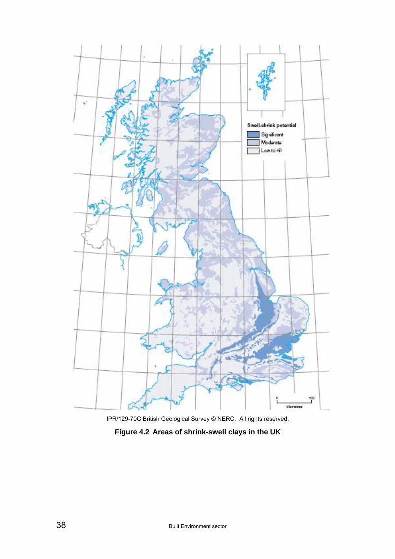
38 Built Environment sector
IPR/129-70C British Geological Survey © NERC. All rights reserved.
Figure 4.2 Areas of shrink-swell clays in the UK

Built Environment sector 39
20,000
25,000
30,000
35,000
40,000
45,000
50,000
55,000
60,000
-40 -20 0 20 40 60
% Change in Summer Rainfall
No
. of
do
me
sti
c s
ub
sid
en
ce
cla
ims
2002
2003
20042005
2006
2007
20082009
Figure 4.3 BE2 Number of domestic subsidence claims versus change in summer rainfall (2002 - 2009)
4.4 BE3 – Overheating of buildings
A response function, quantifying the risk of building overheating, has been developed for England and Wales, as only these countries are covered by the temperature dataset used. Within this version of the CCRA, it was decided to link this metric to workplace productivity and to consider health impacts of overheating elsewhere (including BE1, the Urban Heat Island, and the Heath sector metrics).
Changes in climate are likely to influence both the heating and cooling energy demand within buildings. In the specific case of cooling requirements, longer, drier summer periods may cause overheating in naturally ventilated buildings and affect the capacity of low energy cooling systems to provide comfortable conditions across all building types. The current trend is to rely on mechanical air conditioning to meet additional cooling comfort needs, but the disadvantages of this approach need to be taken into account in any cost-benefit analysis, namely:
likely inhibitive costs of retrofitting within the existing building stock
associated additional energy demand and consequent greenhouse gas emissions
danger of system failure due to power supply interruptions
exhaust heat output resulting in increased external temperatures, especially in an urban environment.
The potential consequences of increased energy demand for cooling are considered in more detail in the energy sector analysis (see Section 4.7).
Overheating occurs when the temperature within a building becomes too hot for the occupants’ thermal comfort. The range of human responses to high temperatures varies from feeling slightly uncomfortable, through loss of productivity, to illness and ultimately heat-related death. The level of response can vary with absolute

40 Built Environment sector
temperatures, the rate of change in maximum temperatures, the persistence of high temperatures and the diurnal temperature range.
Thermal comfort in the domestic environment is important for both health and productivity. High bedroom temperatures result in poor sleep quality and poor performance at work the following day, exacerbated in instances where the work environment is also overheated (Thomas, 1998).
Heat comfort levels within the work environment also influence general productivity at work. Productivity levels have been related to external temperature in a Centre for Economics and Business Research study (CEBR, 2003), which found that productivity falls by 8% at 26°C, by 29% at 32°C and by 62% at 38°C. The respective costs to the UK economy of these productivity falls were estimated at the time as £35m, £126m and £270m per day.
There are still fundamental questions to be addressed with regard to overheating, such as what constitutes overheating, how is it defined and how is it best addressed in a cost-effective manner. This has been identified as a priority area of research by DCLG (DCLG, 2011). The CIBSE overheating task force are also in the process of reviewing their overheating risk criteria.
Current CIBSE guidance (CIBSE, 2006) outlines an overheating threshold of 28°C for any building space with the exceptions of bedrooms where the overheating threshold temperature is 26°C. This threshold should not be exceeded for more than 1% of occupied hours. CIBSE also defines a comfort threshold, which is 3°C lower than the overheating threshold, i.e. 25°C in general and 23°C for bedrooms.
Different buildings will have different responses to external temperature and therefore exhibit widely different degrees of overheating (see for example CIBSE, 2005). The level of risk is affected by multiple aspects of design e.g. thermal mass, air-tightness, ventilation strategy, glazed area (whether shaded or un-shaded) and orientation. It also depends on the usage of the building, the occupancy hours and the building management system.
A detailed quantitative assessment of overheating risk therefore requires not only extensive information relating to building construction and design but also performance data relating to individual building responses. In the absence of such data, external temperature can be used as a proxy for overheating risk in all non-domestic buildings.
The number of days for which the maximum external air temperature reaches or exceeds 26 °C is taken as a response function for building overheating. An external temperature of 26 °C has been used, rather than 28 °C, in order to allow for the effect of solar and internal gains on internal conditions in poorly performing buildings. This is also the temperature at which a reduction in productivity is observed.
This response function gives the number of days each year on which overheating is likely to occur during the day. It does not predict the duration or severity of such overheating. In order to calculate the overheating risk in terms of occupied hours, as defined by CIBSE, hourly temperature data would be required. This more detailed analysis was beyond the scope of this high level overview.
The baseline temperature time series used in this analysis is that developed by Armstrong et al. (2010). To determine the regional temperature time series, daily maximum and minimum temperature time series for stations, reporting on 75% of days between 1993 and 2006, were downloaded from the British Atmospheric Data Centre. The data were processed to obtain population-weighted mean daily series for each region. The AIRGENE algorithm (Ruckerl et al., 2007) was used to avoid spurious fluctuations due to missing data. Only data for Wales and England were available in this dataset.

Built Environment sector 41
Figure 4.4 shows the average number of days for which the external temperature exceeds 26°C for the baseline data period of 1993-2006.
Figure 4.4 Mean number of days per annum at risk of building overheating for the period 1993-2006
Source: Armstrong et al. (2010)
4.4.1 Hospitals
Specific considerations apply to hospital buildings. Their occupants comprise both the healthcare workforce and patients, many of whom are sick and vulnerable. Much hospital accommodation is occupied 24 hours a day, in particular in-patient wards.
In addition to the Building Regulations, design of healthcare facilities is prescribed by a suite of Health Technical Memoranda (HTMs) issued by the Department of Health, which give comprehensive advice and guidance on the design, installation and operation of specialised building and engineering technology used in the delivery of healthcare16. They are applicable to both new and existing sites, and are intended for use during the whole building lifecycle. The Department of Health also produces Health Building Notes, which are “best practice” guidance for healthcare facilities.
Infection control is one of the main drivers of hospital design. Hence high background ventilation rates are recommended: 6 air changes an hour in-patient wards, rising to 25 air changes an hour in operating theatres (HTM 03-01A (2007). There is also a strict hierarchy of cleanliness between different areas, which is maintained with appropriate pressurisation.
Hospitals should also provide a therapeutic environment, which promotes patients’ healing and recovery (e.g. reduced noise, privacy, natural daylight, view of nature).
The NHS estate contains a huge variety of buildings of different ages and functions, even within individual hospital campuses. Overheating is already a problem in some
16 Reference is given to Health Technical Memorandum for England. Similar guidance documents are published for the devolved administrations.

42 Built Environment sector
hospitals, even in new constructions (see for example SHINE Network, 2010). Figure 4.5 shows hourly internal temperatures against external temperatures during Summer 2010 for different buildings and wards on a single hospital campus in England, from initial monitoring studies carried out by the De2RHECC project (De2RHECC, 2010).
A Pre-1939 Nightingale Ward solid construction
B New Modular Ward prefabricated Central corridor with mix of single rooms and 4 bed bays
C 1960s linear framed building with lightweight panel infill Single and multi-bed spaces
Figure 4.5 Monitored hourly internal temperature in summer 2010
Data for three different ward types co-located on the same hospital campus. External temperatures, as shown by the solid blue line, are significantly lower. Source: De2RHECC (2010).
The pre-1939 Nightingale ward (A) is a narrow-plan, naturally ventilated open ward, with high ceilings, large opening windows which allow cross-ventilation and of a solid

Built Environment sector 43
brick/stone construction with high thermal mass. This demonstrates good resilience to external temperature variation in the current climate.
Also shown is a ward of mixed multi- and single-bed rooms in a prefabricated contemporary modular building (B). This is also predominantly naturally ventilated, with fresh air being drawn in through the windows and being exhausted via mechanical extract in the ensuite bathrooms. The NHS favours this type of modern construction, as it can be erected speedily with minimal disruption on site. However it appears less resilient than the older heavyweight Nightingale ward.
The third type of building is a 1960s linear block (C), which is of frame construction with lightweight panel elevation infills. It has some mechanical ventilation. Its performance is problematic in the current climate, with temperatures exceeding 30C even with relatively low external temperatures.
In addition to construction type, several other factors may contribute to overheating.
The air supply is sometimes controlled by a very simplistic algorithm with air supplied at a constant, often high, temperature to all spaces 24 hours a day, regardless of their usage or occupancy. There is an urgent need for improved facilities management.
There is a lack of evidence concerning what the ideal temperature for sleep is or at what temperature sleep is impaired. Wards are often maintained at warmer temperatures than a domestic bedroom overnight. While a rapid night purge, such as might be deployed in offices or schools, is obviously not appropriate in a space where patients are asleep, the current facilities management regime permits very little natural cooling of the building fabric at night. This would only serve to exacerbate the daytime overheating risk.
In new buildings generally, value engineering can result in planned adaptive measures, such as solar shading, being discarded.
For safety reasons, particularly with regard to vulnerable patients, Health Technical Memorandum 55 (HTM 55, 1998) specifies that windows should open to a maximum of 100mm. Furthermore, design considerations may dictate that there is only one opening within a room façade, at the bottom of a casement window; whereas for single-sided natural ventilation, having two separate openings at high and low level is much more effective. These constraints make it extremely difficult to design a natural ventilation strategy which would provide effective protection against overheating.
Changes in use of the space, for example increases in the number of occupants or additional equipment and IT, can all lead to increased internal heat gains.
Health conditions and drug regimes can alter a patient’s physiological perception of temperature in either direction, up or down.
As hospital in-patient wards are occupied 24 hours day, their thermal performance is expected to differ from that of other non-domestic buildings. As explained above, they are likely to be warmer at night and this may compromise occupants’ thermal comfort the following day. Ideally, an overheating response function would be developed for hospitals, which accounts for their special 24-hour occupancy pattern. However there is currently a lack of evidence upon which to base such a metric (see Section 5.6.1).

44 Built Environment sector
4.4.2 Schools
As with hospitals, additional specific guidance for school design is provided by the Department for Education in the form of Building Bulletins. The aim of any school design is to create an environment conducive to learning.
Overheating performance criteria for teaching and learning areas in schools are specified in Building Bulletin 101 (BB 101, 2006).
There should be no more than 120 hours when the air temperature in the classroom rises above 28°C.
The average internal to external temperature difference should not exceed 5°C (i.e. the internal air temperature should be no more than 5°C above the external air temperature on average).
The internal air temperature when the space is occupied should not exceed 32°C.
These standards apply outside the heating season and are for the occupied period of 09:00 to 15:30, Monday to Friday, from 1st May to 30th September. In order to show that the proposed school will not suffer overheating two of these three criteria must be satisfied.
BB 101 also specifies ventilation requirements. The external air supply rate in teaching and learning areas should be a minimum of 3 litres per second per person, with a daily average of 5 l/s per person and the capacity to provide at least 8 l/s per person on demand. The ventilation should limit the concentration of carbon dioxide, resulting from the occupants’ respiration. The maximum carbon dioxide concentration should not exceed 5000ppm during the teaching day and should fall below 1000ppm with the maximum ventilation rate of 8 l/s per person. In the absence of major pollutants, carbon dioxide is taken to be a key indicator for the control of indoor air quality in the classroom. Increased carbon dioxide levels have been shown to have a detrimental effect on pupils’ cognitive performance (Coley, 2004).
Further Building Bulletins specify lighting (BB 90, 1999) and acoustic (BB 93, 2004) requirements. In teaching spaces, the use of natural daylight is preferred. The lighting should provide a balanced distribution of luminance and glare should be avoided. In terms of acoustics, low ambient noise levels are required in order to provide a comfortable teaching environment. The prescribed indoor ambient noise levels should be satisfied even with the maximum 8 l/s per person ventilation rate. External noise levels need to be taken into account when calculating indoor noise levels.
CIBSE TM36 includes case studies of two types of schools. More recent case studies have been carried out on three different school types in London and Manchester (AECOM, 2010). In each case, dynamical thermal simulations were carried out to calculate the risk of overheating both now and in the future (using the CIBSE weather years based on the previous generation UKCIP02 scenarios).
The first type is a Victorian school, with heavyweight solid masonry construction, minimal insulation, single glazing and a pitched slate or tiled roof. Due to the high thermal mass, temperatures can usually be maintained within acceptable limits. However upper floors are at greater risk of overheating due to poorly insulated roofing. The large windows can also lead to high solar gains.
The second school type is a typical 1960s/70s school, with a flat roof, of relatively lightweight construction with single glazing and poor insulation and air tightness. Such schools already severely overheat in the present climate, particularly primary school buildings of this era which are predominantly single-storey.
Built Environment sector 45
The third school type is recently built with medium-weight construction, good insulation and double-glazing throughout. Although built to meet overheating targets, some such schools already experience high temperatures in classrooms between April and September. This may be due to a number of factors, including increased numbers of computers in classrooms and inadequate ventilation.
While there are specific issues with regards to schools, their occupancy is similar to that of many commercial buildings. As with offices, peak occupancy occurs during the daytime, albeit for slightly shorter hours: for pupils, the school day usually ends earlier than the normal working day. Hence the BE3 response function can also be applied to schools. The same caveats hold regarding the variation of thermal response with building construction and management.
4.5 BE5 – Effectiveness of green space
This response function relates the effectiveness of urban green space to changes in relative aridity. Only England is considered. Scotland, Wales and Northern Ireland are not included in the present analysis due to the lack of readily available and comparable datasets.
In the context of the urban system, green and blue infrastructure provides a valuable cooling resource for amelioration of high summer temperatures caused by the urban heat island effect and climate change (Forest Research, 2010). Vegetation cools the surrounding atmosphere by evapotranspiration. In addition, trees provide shading, thus reducing the incidence of direct solar radiation. However, during extremely hot periods, green spaces can become so parched that their evapotranspirative cooling capacity is effectively shut down, as has happened in Hyde Park in London during recent heatwaves. Different habitats and species demonstrate different levels of resilience to drought. Amenity grassland, such as found in urban parks, and shallow-rooting tree species, e.g. beech, are particularly vulnerable (London Climate Change Partnership, 2009a).
The cooling effect of green space has been demonstrated in a number of studies including recent work examining Manchester’s green infrastructure as part of the ASSCUE project (Gill et al., 2007). This study showed that maximum surface temperatures in woodland areas within Manchester were determined to be 12.8°C cooler than town centre areas. Further modelling work suggested that adding 10% green cover to areas such as the town centre or high density residential areas could result in a cooling impact in the range of 2.2 – 2.5°C. Conversely removal of 10% of green cover in the model resulted in a rise in surface temperature of up to 8°C. Provision of green roofs was also shown to provide a beneficial impact in terms of minimising surface temperatures. Tree coverage was highlighted as a key means of providing shading and cooling effects, particularly given its lower sensitivity to prolonged periods of drought than areas of grass that lose their evaporative cooling function fairly quickly.
Data collected as part of the Royal Meteorological Society’s Big Urban Heat Island Experiment in Manchester suggests that the proportion of vegetative cover is directly related to the magnitude of urban heating effects experienced; around half of the temperature variations observed could be attributed to the proportion of vegetation and water within each land-use type (Knight, 2010).
In the case of London, the size of the UHI effect measured for a summer period in 2000 clearly shows the area of Richmond Park being about 1°C cooler than its surroundings (Mayor of London, 2006). The LUCID project team has also explored the relationship between urban land-use fraction and the magnitude of UHI observed. In general a
46 Built Environment sector
larger fraction of green space is a determining factor in the size of UHI; these green spaces need to be large in order to mitigate heat on the city scale. The LUCID team’s simulation filling the entire green space of London with urban land use resulted in temperature increases of a further 3°C (Bohnenstengel et al., 2010 and 2011).
Recent work by CABE has sought to quantify and monetise the cooling capacity of green space (CABE, 2009) in producing a green infrastructure valuation toolbox. This work suggests that a 3% energy saving for each residential property within less than 10 metres of trees is attributable to the shelter provided by the tree canopy. In a similar manner a saving of 8% is achievable in commercial buildings less than 10m from trees (3% for heating and 5% for cooling).
The total area of green space17 in England, broken down by region, is available from the Office of National Statistics (ONS). Clearly the cooling capacity of this green space would be directly affected by prolonged hot, dry periods. As such a response function that considers the total area of green space and a change in relative aridity in England and Wales has been developed. Given the different responses of different species to increasing aridity, and particular microclimates for different urban areas, it is difficult to quantify precisely how the cooling capacity of this green space would be affected. A regional analysis is therefore not appropriate here. However, the present function is considered a proxy for cooling capacity given the progressive damage and death to vegetation resulting from increasing aridity.
Relative aridity provides a measure of how changes in average annual temperatures and rainfall will affect the likelihood of dry periods. Relative aridity scores (RAS) have been calculated as part of the water sector analysis (risk metric WA1) using the equation:
9061
9061
9061
9061 6.04.0Re
RainSD
RainRain
TSD
TTScoreAriditylative futurefuture
where futureT is the average of annual temperatures over a given period in the future,
9061T and 9061TSD are the average and standard deviation over the 30-year period.
futureRain is the average of annual totals, over a given period in the future, 9061Rain
and 9061RainSD are the average and standard deviation over the 30-year period.
As the RAS is a normalised score, values of between plus and minus one can be regarded as ‘normal’ with respect to the 1961-1990 climate; values greater than one ‘more arid’ than normal and values greater than two as ‘extremely arid’ compared to 1961-1990. Although the RAS scores developed for England and Wales are used, the measure can be taken as indicative of change for England.
The Water sector analysis calculated RAS for the period 1766 to 2003 using the Central England Temperature (CET) and the England and Wales rainfall series (Met Office). A number of major drought episodes were identified during the 20th century (Cole and Marsh, 2005). Of these, the drought of 1921/22, which is recognised as the worst resources drought for the Thames basin, has the highest RAS of 2.59. The year of the recent catastrophic European heatwave, 2003, has the second highest RAS at 1.77.
A basic relationship between relative aridity and effective area of green space has been proposed as shown in Figure 4.6. This assumes a linear decline in the effectiveness of green space once relative aridity exceeds the normal upper limit of 1.
17 Green space is defined in the Generalised Land Use Database (http://www.communities.gov.uk/documents/planningandbuilding/pdf/154941.pdf)
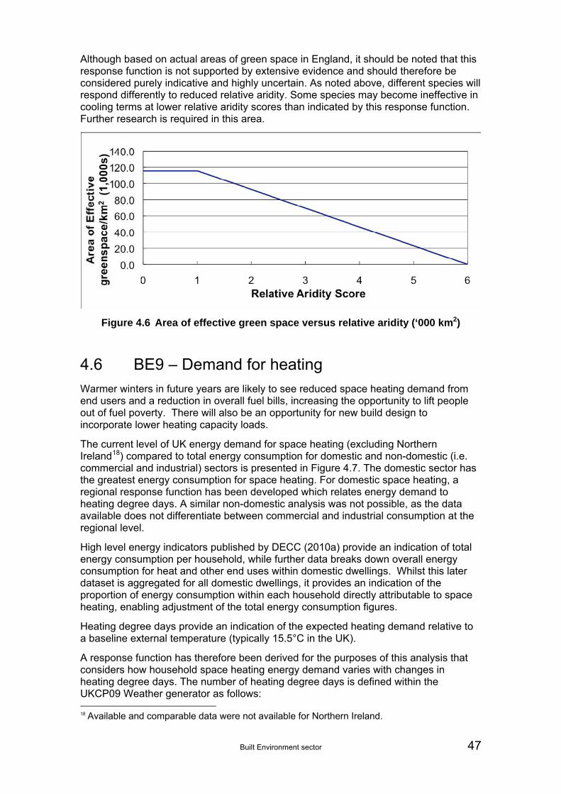
Built Environment sector 47
Although based on actual areas of green space in England, it should be noted that this response function is not supported by extensive evidence and should therefore be considered purely indicative and highly uncertain. As noted above, different species will respond differently to reduced relative aridity. Some species may become ineffective in cooling terms at lower relative aridity scores than indicated by this response function. Further research is required in this area.
Figure 4.6 Area of effective green space versus relative aridity (‘000 km2)
4.6 BE9 – Demand for heating
Warmer winters in future years are likely to see reduced space heating demand from end users and a reduction in overall fuel bills, increasing the opportunity to lift people out of fuel poverty. There will also be an opportunity for new build design to incorporate lower heating capacity loads.
The current level of UK energy demand for space heating (excluding Northern Ireland18) compared to total energy consumption for domestic and non-domestic (i.e. commercial and industrial) sectors is presented in Figure 4.7. The domestic sector has the greatest energy consumption for space heating. For domestic space heating, a regional response function has been developed which relates energy demand to heating degree days. A similar non-domestic analysis was not possible, as the data available does not differentiate between commercial and industrial consumption at the regional level.
High level energy indicators published by DECC (2010a) provide an indication of total energy consumption per household, while further data breaks down overall energy consumption for heat and other end uses within domestic dwellings. Whilst this later dataset is aggregated for all domestic dwellings, it provides an indication of the proportion of energy consumption within each household directly attributable to space heating, enabling adjustment of the total energy consumption figures.
Heating degree days provide an indication of the expected heating demand relative to a baseline external temperature (typically 15.5°C in the UK).
A response function has therefore been derived for the purposes of this analysis that considers how household space heating energy demand varies with changes in heating degree days. The number of heating degree days is defined within the UKCP09 Weather generator as follows: 18 Available and comparable data were not available for Northern Ireland.

48 Built Environment sector
∑ (15.5 – daily mean temperature) whenever mean temperature < 15.5 ºC. This assumes both the daily Tmax and Tmin are < 15.5 ºC and in other cases weighted increments are used.
Thus if, on a given day, the mean temperature is 5.5ºC, the number of heating degree days for that day would be 10. Hence, it is quite possible that the number of heating degree days in a year exceeds the number of days in the year.
The relationship between heating consumption and heating degree days is presented in Figure 4.8. It should be noted that an increase in mean average daily temperatures would see a reduction in heating degree days and a move from right to left on the response function.
Figure 4.7 UK Energy Consumption in 2009 by sector
Source: DECC (2010a) data

Built Environment sector 49
0
2,000
4,000
6,000
8,000
10,000
12,000
14,000
16,000
18,000
20,000
0 500 1,000 1,500 2,000 2,500 3,000
Number of Heating Degree Days per year
Sp
ac
e H
ea
tin
g E
ne
rgy
Co
ns
um
pti
on
Pe
r H
ou
se
ho
ld
(kW
h/y
r)
North East England
North West England
Yorkshire & The Humber
East Midlands
West Midlands
East of England
London
South East England
South West England
Wales
East Scotland
North Scotland
West Scotland
Figure 4.8 Space heating energy demand versus heating degree days (by region)
4.7 EN2 – Energy demand for cooling
To create a response function for cooling demand, the risk metric Cooling Degree Days (CDD) is used. CDD is the most common climatic indicator of the demand for cooling services and is a measure of the average temperature’s departure from a certain base temperature. It is assumed that, if air temperatures are below the base temperature, no energy for cooling is required. In this UK analysis, CDD is defined as the day-by-day sum of the mean number of degrees by which the air temperature is more than a value of 22°C and calculated using the method set out by Jenkins et al. (2009).
Analysing future projections of CDD therefore provides a means to assess how cooling demand may change in the future based on climatic factors alone. In this study, projections of future cooling demand were made using both the CDD approach and recent research (Section 5.9).
4.8 WA5 and WA6 - Water supply-demand deficit and population affected
The supply-demand balance is calculated based on the water available in surface water and groundwater and the demand for water. There is no response function required for the supply-demand metrics. Instead the results for these metrics were calculated through the use of simple supply-demand balance models. This includes the population affected by supply-demand deficits. These were developed at the UKCP09 river basin region scale, with one spreadsheet for each region in the UK.
The models use the following data:
Ofwat June Return data
Deployable Output
Demand for water – per capita consumption

50 Built Environment sector
Change in population.
June Return reports were either downloaded from Ofwat, or obtained directly from water companies. Data on the security of supply index and applications for vulnerable customer status were extracted from each report and collated in a database to form a baseline for the study (see Rance et al. (2012) for more details).
The models work by using the data to obtain results for each of the emissions scenarios, for each time period. Climate change affects household demand and supply but detailed climate impact models were not developed for other components, such as leakage or ‘outage.’ The outputs of this metric are also based on the assumption that there is no intervention in terms of implementing demand or supply-side measures.
4.9 FL6, FL7 and FL13 - Flooding of properties
Response functions in the Floods and Coastal Erosion sector were based on river and tidal flood modelling for England and Wales. The process of using the model results to develop the functions is described in the Floods and Coastal Erosion sector report (Ramsbottom et al., 2012). The functions were developed separately for Wales and the English Areas and include both numbers of properties and Expected Annual Damage (EAD).
FL6 - Residential properties at significant likelihood of flooding (FL6a: number; FL6b: EAD)
The response functions have been calculated using the number of residential properties by region and the associated EAD. The functions have been calculated for tidal and river flooding but not surface water flooding.
Examples of response functions are shown on Figure 4.8 (number of residential properties at risk of river flooding) and 4.9 (Expected Annual Damages (EAD) for residential properties caused by river flooding). ‘Significant likelihood’ of flooding corresponds to an annual probability of 1.3% (or once in 75 years on average).
Number of residential properties at significant likelihood of flooding (river)
0
20
40
60
80
100
120
0.00 0.05 0.10 0.15 0.20 0.25 0.30 0.35 0.40 0.45 0.50 0.55 0.60
Th
ou
sa
nd
s
Relative Change in Peak Flow
Nu
mb
er
of
pro
pe
rtie
s
1. East Midlands
2. East of England
3. London
4. North East England
5. North West England
6. South East England
7. South West England
8. Wales
9. West Midlands
10. Yorkshire and Humberside
Figure 4.9 Residential properties at significant likelihood of river flooding

Built Environment sector 51
Expected Annual Damage to residential property (river flooding)
£-
£100,000
£200,000
£300,000
£400,000
£500,000
£600,000
0.00 0.05 0.10 0.15 0.20 0.25 0.30 0.35 0.40 0.45 0.50 0.55 0.60
Th
ou
sa
nd
s
Relative Change in Peak Flow
Ex
pe
cte
d A
nn
ua
l D
am
ag
e 1. East Midlands
2. East of England
3. London
4. North East England
5. North West England
6. South East England
7. South West England
8. Wales
9. West Midlands
10. Yorkshire and Humberside
Figure 4.10 EAD for residential properties: river flooding
FL7 - Non-residential properties at significant likelihood of flooding (FL7a: number; FL7b: EAD)
The response functions have been calculated using counts of the number of non-residential properties by region and the associated EAD. The functions have been calculated for tidal and river flooding but not surface water flooding.
FL13 - Residential properties at significant likelihood of flooding (to assess insurance impacts)
This metric is used to provide an indication of the impact of increases in flood risk on property insurance. This is based on the response function for metric FL6a (Number of residential properties at significant likelihood of flooding). Figure 4.9 shows the response function for river flooding.
4.10 HE1 – Temperature mortality (Heat) and HE5 Temperature mortality (Cold)
The analysis of these metrics is mainly based on two papers: Hajat et al. (2007) who considered both heat and cold related deaths over the period 1993-2003, and Armstrong et al. (2010) who considered just heat related deaths over the period 1993-2006. Both papers considered an epidemiological time series of daily mortality rates and daily mean or maximum temperatures for regions in England and Wales.
Based on the analysis carried out, both papers presented regional current-day exposure-response functions (including confidence bands) linking excess daily mortality (heat related), or premature deaths, correlated against daily mean or maximum temperature, population and a baseline mortality rate for each region. Hajat et al. (2007) also showed the same relationship for cold related mortality, or premature deaths avoided.
For this analysis, it is assumed that these current-day exposure-response functions do not change over the rest of the century, as there is insufficient published evidence on the effects of autonomous and planned adaptation on temperature-related mortality. The Health sector report applies the response functions set out in Hajat et al. (2007) and Armstrong et al. (2010) for the regions in England and Wales. For Scotland and Northern Ireland, the heat and cold slopes corresponding to the North East and North
52 Built Environment sector
West of England respectively were used. These regions were considered the most representative of Scotland and Northern Ireland and provide a conservative estimate of heat and cold related mortality.
4.11 HE2 – Temperature morbidity (Heat) and HE6 Temperature morbidity (Cold)
There is evidence that both very high and very low temperatures have an impact on a range of morbidity outcomes. Morbidity rises in hot weather, particularly in the elderly, very young and sick people (Vassallo et al., 1995). Elderly people are vulnerable to heat stress, especially those in hospital or long-term care institutions.
A selection of studies summarised in the Health sector report show that generally hotter climatic conditions and more frequent and intense heatwaves are likely to cause an increase in patient-days per year in hospital in the UK due to heat-related illness (i.e. hospital admissions attributable to high temperatures but not necessarily diagnosed as hyperthermia, heat stroke, etc.).
The rate of change is more uncertain than that of heat-related mortality (probably because many heat-related deaths occur before the sufferers come to medical attention), and little work has been carried out in this area. However, Donaldson et al. (2002) indicates a linear relationship between heat related mortality and heat related patient-days which they calculated as 1 death for every 102 patient days in hospital. Although this figure can be considered highly uncertain due to the very limited published evidence, it is the only known indication of an exposure-response function for this metric in the UK. Nevertheless, this empirical relationship between heat-related deaths and hospital patient days per year in the UK obtained from the Donaldson et al. (2002) study has been used to make quantitative estimates of heat related morbidity for illustrative purposes only.
Heat related morbidity is therefore tentatively determined by multiplying the heat related mortality deaths (HE1) by a factor of 102. The same factor is also used to estimate the reduction in cold-related hospital patient days per year resulting from milder winters (HE6).
4.12 HE3 – Flood related deaths
The Health sector report (Hames and Vardoulakis, 2012) provides detailed discussion of how response functions have been developed to provide estimates of future mortality rates due to fluvial and tidal flooding including violent wave overtopping.
An assessment of past flood events in the UK, together with recent flash flood events in Western Europe from the EMDAT database, indicates an average mortality rate due to fluvial flooding of approximately 3 per year. In view of the potential for very severe flash floods as well as more minor flood events, some of which may not be widely reported or necessarily attributed to extreme flood events, an average fatality rate of between 5 and 10 per year is considered likely. A fatality rate of 8 per year has therefore been adopted for this analysis.
For coastal flooding, an average fatality rate has also been established through examination of previous events. Severe but very rare coastal flooding events could potentially lead to hundreds of deaths. For example, there were over 300 deaths in 1953. However the average yearly rate is small, possibly in the region of about 2 to 5 per year, and a central estimate of 3 has been assumed for this analysis. This

Built Environment sector 53
relatively small number compared with deaths from other causes, for example heat waves, demonstrates that the number of deaths as a result of extreme event coastal flooding is not anticipated to be large.
As part of an unofficial data gathering process for the Violent Overtopping of Waves at Seawalls Project (http://www.vows.ac.uk/), a record of deaths due to overtopping of water of seawalls or land recorded in the media has been kept. Although this provides only a limited sample of data, the study suggests a baseline rate of fatalities due to overtopping of 7 per year. For future risk, fatalities would be expected to be related to the increase in wave activity nearshore, which in turn due to depth limited effects, can be considered a function of sea level rise. The analysis provides a response function that estimates an exponential increase in deaths due to overtopping as sea level rises.
Thus the total baseline number of deaths per year is 18. Response functions are provided in the Health sector report for these three different causes of mortality from flooding and storms.
4.13 BU6 – Increased exposure for mortgage lenders
Climate change is projected to cause an increase in flood probability to properties, including flooding from tidal, fluvial and surface water sources (Pitt, 2008). As the probability of flooding increases, insurance for properties that flood may be increasingly costly or difficult to obtain in certain circumstances. There are already cases in the UK where property insurance is either not obtainable or very expensive.
For the purposes of this analysis, the number of residential properties at significant likelihood of tidal and river flooding is used as an indicator of the impact of flooding on the availability of insurance, and consequently on the gross level of mortgage lending exposed (metric FL6a, see Section 4.9). Here, the baseline (current) sea level and river flow peak data are used to derive the existing level of significant likelihood of flooding to properties in different regions (by numbers of properties).
This total mortgage fund value at risk is then calculated based on the total value of mortgages for residential properties at significant likelihood of flooding and taking into account the possible proportion of value that may be affected. Full details of the analysis are provided in the Business sector report (Baglee et al., 2012).
4.14 BU10 – Loss of staff hours due to high internal building temperatures
BE3, overheating of buildings, has been extended to consider the implications of overheating on productivity in the work place. The combination of overheating and warm weather periods has been observed to produce two responses in the workforce; increased absenteeism (Kronos, 2007) and reduced productivity (Parsons, 2009). The fall in productivity when working in high temperatures has been examined by the National Institute of Occupational Safety and Health in the US (cited by CEBR, 2003; NIOSH, 1986) and a response function based on an interpretation of their estimates is presented in Figure 4.11 (left plot).

54 Built Environment sector
25 30 35 400
20
40
60
80
Temperature (deg C)
Fal
l in
prod
ucti
vity
(%
)
0 10 20 3010
20
30
40
time (hr)
Tem
pera
ture
(de
g C
)
26
Figure 4.11 Fall in productivity as a function of temperature Interpreted from NIOSH (1986) estimates (left plot). The function is used to estimate the duration above
the threshold based on minimum, maximum and mean daily temperatures (red line), compared with observations (blue dotted line) for a typical hot day19 (right plot).
The relationship between fall in productivity and temperature has been used with some scaling components to take into account applicability within the UK, as the response function for this metric. Full details are provided in the Business sector report (Baglee et al., 2012).
19 Based on observed air temperatures in Southampton on 27 June 2010 (source: www.sotonmet.co.uk)

Built Environment sector 55
5 Estimates of Change with Selected Climate Scenarios
5.1 Introduction
The purpose of this step is to apply the UKCP09 projections to the response functions developed in Section 4 in order to estimate their evolution under different future scenarios. It is based on scaling using the relevant climate variable(s) and/or expert opinion and provides consistent assessment in the context of the UKCP09 projections.
The results presented in this section only consider climate change sensitivity. No change is made to the current socio-economic baseline. Social and economic drivers are only introduced in Section 6.
M Confidence assessment from high (H) to low (L)
3 High opportunity (positive)
2 Medium opportunity (positive)
1 Low opportunity (positive)
1 Low risk (negative)
2 Medium risk (negative)
For each metric a scorecard is given at the start of each section to indicate the confidence in the estimates given and the level of risk or opportunity. Confidence is assessed as high (H), medium (M) or low (L). Risks and opportunities are scored either high (3) medium (2) or low (1) (shown to the right). These are given for the lower (l), central (c) and upper (u) estimates for the 2020s, 2050s and 2080s. Further information is provided in Appendix 3. Where estimates are uncertain, or no data is available, this is stated in the scorecard. 3 High risk (negative)
5.2 Data used
The following data were used in the estimation of the impact of climate change with selected climate scenarios:
Mean average daily temperature (degrees Celsius) over the period 1990 – 2009: data supplied by the Met Office (to provide baseline information).
Change in population for the water supply-demand balance: based on data taken from the ONS.
5.3 Use of UKCP09
The full UKCP09 data set was downloaded from the internet20, for the 2020s, 2050s and 2080s, for the Low, Medium and High emissions scenarios. The following variables were used:
20 http://ukclimateprojections-ui.defra.gov.uk

56 Built Environment sector
Change in minimum air temperature: summer (degrees Celsius) (Change in future 30-year average of seasonal minimum air temperature at 1.5m from the baseline climate (1961-1990) long-term average).
Change in mean annual temperature (degrees Celsius) (Change in future 30-year average of annual average air temperature at 1.5m from the baseline climate (1961-90) long term average).
Change in mean average air temperature: summer (degrees Celsius) (Change in future 30-year average of seasonal maximum air temperature at 1.5 metres from the baseline climate (1961-1990) long-term average).
Change in mean average air temperature: spring (degrees Celsius) (Change in future 30-year average of seasonal maximum air temperature at 1.5 metres from the baseline climate (1961-1990) long-term average).
Change in mean average air temperature: autumn (degrees Celsius) (Change in future 30-year average of seasonal maximum air temperature at 1.5 metres from the baseline climate (1961-1990) long-term average).
Change in mean average air temperature: winter (degrees Celsius) (Change in future 30-year average of seasonal maximum air temperature at 1.5 metres from the baseline climate (1961-1990) long-term average).
Change in summer period precipitation (%) (Change in future summer average precipitation from the baseline climate (1961-90) long term average).
5.4 BE1 – Urban Heat Island
Summary Class
2020s 2050s 2080s Metric code
Metric name
Co
nfi
den
ce
l c u l c u l c u
BE1 Urban Heat Island H Too uncertain21
Several factors may contribute to the future intensification of the UHI. Climate change impacts, such as rising average temperatures, more frequent and intense heatwaves and more cloud-free days, will increase the amount of heat within the urban area. Drier summers may also lead to loss of evaporative cooling from green infrastructure (see BE5 Effectiveness of Green space). An increase in population density may lead to urban creep and loss of permeable green space. Anthropogenic heat emissions already contribute to the summer UHI within London, but this could increase in future if air-conditioning is widely adopted, (for example in the domestic sector).
Urban effects are not included in the UKCP09 projections. Therefore the Urban Heat Island effect is not explicitly represented, either in the baseline data or in the future. Nonetheless, urban temperatures would be expected to rise in line with the projected temperature increase. In London, for example, a 1.6°C rise in summer minimum air temperature is projected under the p50 Medium emissions scenario by the 2020s; this is projected to rise to 2.9°C and 4.1°C under the same scenario by the 2050s and 2080s respectively. Projected changes in summer minimum air temperatures under
21 BE1 is too uncertain to assess UK-wide but has high confidence as the magnitude is site specific
Built Environment sector 57
different scenarios are summarised in Table 5.1. These figures may underestimate the overall change in temperatures in urban areas, as they are summer averages and therefore do not consider extremes, such as during a heat wave when the UHI intensity is greatest.
Minimum night-time temperatures are an important factor in determining levels of heat stress which may be harmful to health. The precise health consequences of higher night-time temperatures is an area of ongoing research (e.g. Dousset et al., 2011). Nevertheless, a guide as to when night-time temperatures trigger potential negative health consequences amongst the vulnerable is provided in present heat wave planning guidance; threshold day and night temperatures are defined by the Met Office for each region of England in the Heatwave Action Plan as summarised in Table 5.2.
UKCP09 projections for mean average night-time summer temperature under the p50 Medium emissions scenario are shown in Figure 5.1. It is interesting to note that by the 2080s under this scenario the current threshold temperature would be below the projected average night-time temperature in some parts of Southern England and Wales. Given the UKCP09 projections of Figure 5.1 it is likely that an increased frequency of night-time temperature heat wave action triggers would occur in London and the South East by the 2020s. The frequency of heat stress events would also increase in other regions of England and Wales, with a northwards shift by the 2050s and beyond.
Over time, some physiological and behavioural adaptation to increased temperatures would be expected, as reflected in the regional variation in the action plan threshold temperatures, but the extent of such human adaptation is difficult to quantify. Nevertheless, it is still anticipated that heat stress would become an increasing problem in the event of a warmer climate. Heat-related health consequences and the potential for physiological adaptation are considered in more detail in the Health sector report and are summarised elsewhere in this report.

58
Table 5.1 Projected change in summer minimum air temperature
2020s 2050s 2080s
Medium Medium Medium Low Low Medium High High Low Low Medium High High
UKCP09 Region p10 p50 p90 p10 p50 p50 p50 p90 p10 p50 p50 p50 p90
East of England 0.6 1.5 2.7 1.1 2.5 2.7 3.1 5.3 1.3 3.0 3.9 5.0 8.4
East Midlands 0.6 1.5 2.6 1.1 2.4 2.7 3.1 5.2 1.3 2.9 3.8 4.9 8.2
London 0.6 1.6 2.9 1.2 2.7 2.9 3.4 5.6 1.4 3.2 4.1 5.4 9.0
North East 0.5 1.4 2.6 1.0 2.2 2.5 2.8 4.8 1.1 2.7 3.6 4.6 7.7
North West 0.5 1.5 2.6 1.0 2.3 2.5 2.9 4.9 1.1 2.7 3.6 4.6 7.8
South East 0.6 1.7 2.9 1.2 2.7 2.9 3.4 5.7 1.4 3.2 4.2 5.4 9.1
South West 0.5 1.6 2.9 1.0 2.5 2.9 3.3 5.5 1.2 3.1 4.1 5.3 8.8
West Midlands 0.5 1.5 2.7 1.0 2.4 2.7 3.1 5.2 1.2 2.9 3.9 5.0 8.4
Yorkshire and The Humber 0.6 1.5 2.5 1.1 2.3 2.6 3.0 4.9 1.2 2.8 3.7 4.7 7.9
Eastern Scotland 0.6 1.5 2.5 1.1 2.3 2.5 2.9 4.9 1.2 2.8 3.7 4.6 7.7
Northern Scotland 0.5 1.3 2.5 0.9 2.1 2.3 2.6 4.4 1.1 2.6 3.3 4.2 6.9
Western Scotland 0.5 1.4 2.5 0.9 2.1 2.4 2.7 4.6 1.0 2.6 3.5 4.4 7.4
Northern Ireland 0.4 1.4 2.5 0.9 2.1 2.4 2.8 4.6 1.2 2.6 3.6 4.5 7.4
Wales 0.5 1.5 2.6 0.9 2.3 2.6 3.0 5.0 1.1 2.8 3.8 4.9 8.0
Channel Islands 0.4 1.5 2.8 1.0 2.4 2.7 3.1 5.2 1.2 2.9 4.0 5.0 8.4
Isle of Man 0.4 1.3 2.3 0.8 2.0 2.2 2.5 4.3 0.9 2.4 3.2 4.1 6.9
Source: UKCP09 change in minimum air temperature – summer (degrees Celsius) (Change in future 30-year average of seasonal minimum air temperature at 1.5m from the baseline climate (1961-1990) long-term average).

Built Environment sector 59
Table 5.2 Heatwave Action Threshold Temperatures
Region Day Temperature (°C) Night Temperature (°C)
London 32 18
South East 31 16
South West 30 15
Wales 30 15
Eastern 30 15
West Midlands 30 15
East Midlands 30 15
North West 30 15
Yorkshire and Humber 29 15
North East 28 15
Source: Department of Health and Welsh Government, 2010
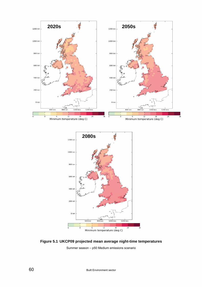
60 Built Environment sector
2020s 2050s
2080s
Figure 5.1 UKCP09 projected mean average night-time temperatures
Summer season – p50 Medium emissions scenario

Built Environment sector 61
5.4.1 Urban Heat Island and climate change research
The spatial scale in the UKCP09 regional climate change models is too large for urban heat islands to be represented explicitly. Understanding the future evolution of the UHI under climate change is an active and rapidly evolving area of research. The EPSRC has funded a number of research programmes in this area, including LUCID (focussed on London) and SCORCHIO (focussed on Greater Manchester). A number of ‘downscaling’ models have been developed in order to deepen understanding of the UHI and also to disaggregate climate change from other contributing factors such as green infrastructure and anthropogenic heat emissions. Unfortunately final results from these valuable projects were not yet available at the time of the CCRA Tier 2 analysis. It is only more recently that they have been disseminated. A brief overview of their outputs is given here.
In the ARCADIA project, a new version of the Met Office Hadley Centre’s regional climate model that includes the effects of land surface and anthropogenic heat emissions was coupled with a weather generator to analyse temperature in London under current and future conditions (Hall et al., 2009). The results suggest that:
By the 2050s, one third of London's summer may exceed the Met Office current heat wave temperature threshold.
Land use planning has a notable effect on the number of people exposed to heat waves, but is much less important than the change in climate.
A threefold increase in anthropogenic heat emissions (e.g. from air conditioning) on top of climate change has a negligible impact on maximum day-time temperature, but would raise minimum night-time temperatures by about 0.5°C which would aggravate heat stress.
Similarly, within the SCORCHIO project, adapted versions of the Hadley Centre climate models (the global model HadAM3 and more recently the regional model HadRM3), which include urban and other land surface properties and anthropogenic heat sources, have been used to explore local urban heat island effects (McCarthy, 2010). Outputs from the regional model provide an indication of where UHI effects are projected to significantly influence night-time temperature in the UK, as illustrated in Figure 5.2 which shows projected increases compared with the baseline used for UKCP09 (of 1961-90). This would suggest that the major consequences are likely to be experienced in the Greater London and Greater Manchester areas in the time horizon to the 2050s (McCarthy et al., 2011).
The SCORCHIO project has also developed a method for combining the outputs of the regional climate models with the UEA Weather Generator to create synthetic daily time series of weather variables (including temperature and rainfall) at 5 km resolution, with an improved representation of the UHI.
Results from the SCORCHIO models show that, in the UK, urban and rural areas are warming at the same rate. There is no increase in the intensity of the UHI as a result of projected changes in climate. However, UHI intensity alone is not a useful gauge of the potential impacts of urban climate change, which will be most strongly felt during extreme events. An extreme heat island event during relatively cool conditions will be less significant for human comfort than a small heat island during a heat wave for example. Therefore, although UHI intensity does not necessarily increase under climate change, the UHI does exacerbate the frequency of extreme heat events as experienced by urban dwellers.
These new climate projections for urban areas are being used in building simulation models to provide information about the risk of overheating. They also form the basis of a GIS-based city-scale hazard model, SCHEEME (Sustainable Cities Heat, Energy and

62 Built Environment sector
EMissions Evaluation). The SCHEEME model incorporates all elements of the SCORCHIO project and allows modelling of future climate risk and vulnerability, especially health and human comfort (i.e. overheating), within urban areas.
Following on from SCORCHIO, the COPSE project (which is currently ongoing) has collected detailed temperature data within the Greater Manchester urban area and has produced a tool to modify UKCP09 data to include UHI effects.
The LUCID project has developed a suite of urban climate models, which run at city, neighbourhood and street scales respectively in order to quantify the effect of urbanisation processes on local environmental conditions. A further suite of impact models has also been developed in order to investigate the impact of such conditions on comfort, energy use and health.
The LUCID city-scale urban climate model demonstrates that urban land-use distribution is key to urban temperatures; the current scattered greening in London has a cooling effect on the city. However, in order to affect the city-scale UHI the greening needs to be extensive. Winds are also an important cooling mechanism.
Building form has a moderate impact on urban temperatures. Increasing the surface albedo, with white roofs for example, leads to daytime cooling. At present, the UHI significantly reduces winter heating demand and thus has a net energy benefit for London. However, this balance could be tipped if air-conditioning is widely adopted, for example in domestic buildings. In this scenario, anthropogenic heating is likely to be a significant contributor to the UHI effect in summer.

Built Environment sector 63
Projected minimum temperature without urban heat island effects
Projected minimum temperature with urban heat island effects included
Difference between the two projections Source: Met Office Hadley Centre (© Crown copyright)
Figure 5.2 Increase in minimum temperature (°C) in period 2041 – 2050
Compared with 1961-90 baseline, based on Met Office modelling

64 Built Environment sector
5.5 BE2 – Subsidence
Summary Class
2020s 2050s 2080s Metric code
Metric name
Co
nfi
den
ce
l c u L c u l c u
BE2 Subsidence M 1 1 2 1 2 2 1 2 2
The change in the projected number of household incidents of subsidence under the different climate change scenarios considered in this study is summarised in Table 5.3. It should be noted that this analysis is based upon change to summer rainfall and hence may underestimate the overall impact.
Based on the response function developed in Section 4.3, an increase in the number of incidents of subsidence is projected in all regions where shrink-swell soils are present under a p50 Medium emissions scenario. This reflects a reduction in summer precipitation and the increased likelihood of prolonged drier spells in summer months.
For example, the average increase in the number of houses suffering subsidence in regions with shrink-swell clay soils is projected to be about 17% by the 2050s under a p50 Medium emissions scenario. This ranges from a reduction of about 10% to an increase of about 30% for the range for climate change scenarios used in the analysis. The results in Table 5.3 show that the range of projections is wide, reflecting the uncertainty in the projected changes in summer precipitation. For example, for all p90 scenarios (i.e. those with the highest amount of rainfall in the summer) the potential risk of subsidence is projected to reduce.
There is likely to be a degree of autonomous adaptation associated with this impact, thereby potentially reducing the overall increase in risk. Subsidence resulting from shrink-swell incidents is most likely to affect older dwellings with less resilient foundations. New developments in high-risk areas are required by Building Regulations to demonstrate sufficient resilience in their design to withstand ground movements. As a result, despite projected population increases in a number of the regions where shrink-swell soils are present, and a consequential increase in housing numbers, new developments should not increase the risk of additional subsidence incidents. Furthermore replacement of existing aged stock is likely to reduce the risk of incidents (although this effect will be limited given current replacement rates).

65
Table 5.3 Projected number of domestic subsidence incidents per annum
2020s 2050s 2080s
Medium Medium Medium Low Low Medium High High Low Low Medium High High
UKCP09 Region 2008
baseline P10 p50 p90 p10 p50 p50 p50 p90 p10 p50 p50 p50 p90
East of England 6,114 7,426 6,499 5,427 8,016 6,818 7,084 7,122 5,694 8,141 6,901 7,299 7,635 5,805
East Midlands 1,365 1,642 1,445 1,212 1,767 1,513 1,569 1,578 1,273 1,797 1,528 1,616 1,682 1,297
London 17,413 21,486 18,635 15,068 23,261 19,562 20,376 20,489 15,948 23,648 19,869 21,042 22,049 16,308
North East - - - - - - - - - - - - - -
North West - - - - - - - - - - - - - -
South East 3,823 4,734 4,090 3,329 5,116 4,319 4,496 4,521 3,520 5,197 4,367 4,637 4,850 3,610
South West 824 1,023 882 721 1,112 934 975 982 756 1,131 946 1,009 1,058 781
West Midlands - - - - - - - - - - - - - -
Yorkshire and The Humber
161 195 173 147 212 183 189 189 157 215 187 196 203 162
Scotland - - - - - - - - - - - - - -
Northern Ireland - - - - - - - - - - - - - -
Wales - - - - - - - - - - - - - -
Notes: 1 Blank entries denote regions where no clay soils with significant shrink-swell potential are present and therefore the risk of subsidence is much lower. 2 p90 is wetter than p10 and therefore has a lower projected number of subsidence incidents.

66 Built Environment sector
5.6 BE3 – Overheating of buildings
Summary Class
2020s 2050s 2080s Metric code
Metric name
Co
nfi
den
ce
l c u l c u l c u
BE3 Overheating of buildings H 1 2 2 2 2 3 2 3 3
The projected changes in daily maximum temperature for the UKCP09 scenarios have been added to the baseline temperature dataset of Armstrong et al. (2010). The method described in Section 4.4 (i.e. counting the number of days above a threshold for each scenario) has then been applied and an estimated change in the number of days at risk of overheating in non-domestic buildings under each climate scenario calculated. The outcomes are summarised in Table 5.4.
This metric has been restricted to non-domestic buildings because data are available on the main issues of maximum day-time temperatures and work place productivity. The issues for domestic buildings are more difficult to assess and include both day-time and night-time discomfort during periods of high temperatures. Mortality and morbidity impacts on people caused by heat were assessed in the Health sector and have been included elsewhere in this report.
It should be noted that the method of calculation used assumes that the current pattern of daily variability in maximum temperature will persist. The UKCP09 projection for change in maximum temperature is also applied uniformly across each season and region. This also assumes that there is no change in the underlying weather pattern and that the diurnal variation is constant from day to day (which is clearly not the case).
The results suggest that increased risk of overheating is a very real threat under all except the lowest p10 scenarios. The risk increases towards the South and East. Unsurprisingly, the highest risk occurs in London. By the 2020s, the risk of overheating is projected to approximately double under the p50 Medium emissions scenario. By the 2050s the number of days for which the maximum temperature is 26°C or more is projected to increase by values ranging from 11 days in the North East to 32 days in London under the Medium emissions p50 scenario.
By the 2080s, under the Medium emissions p50 scenario, a maximum daily temperature of 26°C or above is projected to occur on approximately 30 days a year in the northerly regions and Wales and on about 70 days a year in London (baseline of 18 days plus a projected increase of 51 days). Under the high p90 scenario, a maximum daily temperature of 26°C or more is projected to occur on about 80 days in the North East and about 120 days (i.e. 4 months) in London. This indicates that such high daily maxima could become the norm during summer.
These results do not discriminate between rural and urban areas. However, the baseline Tmax dataset of Armstrong et al. (2010) is population weighted. Hence one would expect it to provide a reasonable baseline for urban areas. This analysis also excludes night-time minimum temperatures, which are important in the Urban Heat Island effect and critical for buildings such as hospitals22, which are continuously occupied.
22 Consideration could be given developing a more sensitive response function for hospital overheating in the future.

Built Environment sector 67
At present energy efficiency is being driven by winter heating rather than summer cooling. However, given that working environments are typically in use during the hottest part of the day, they also have to consider maximum daytime temperatures. Clearly building form is a major influence on the risk of significant overheating; vulnerable building types include:
Modern highly insulated lightweight buildings. The lack of exposed thermal mass in these structures means that, during hot days, they have neither the capacity to soak up heat gains, nor any thermal mass to act as a source of ‘coolness’.
Buildings with excessive south and west facing glazing, where incident solar radiation creates major solar gains.
Older buildings, which have high thermal mass and smaller shaded windows, would in general be less vulnerable, if used correctly.
‘Mixed mode’ design, where passive cooling measures are used in the first instance, with mechanical ventilation used only as a back-up, is likely to become increasingly important given wider targets to reduce overall energy consumption and associated carbon emissions. There is, however, always the danger that any ‘back-up’ cooling will be used much more frequently than intended. Discouraging extensive use of mechanical air conditioning would also avoid maladaptation in the form of significant additional exhaust heat from buildings, which would exacerbate local urban heating effects.
In terms of new build design therefore, there is potential to reduce the risk of overheating through appropriate adaptive design. This could be driven primarily by Building Standards to ensure widespread uptake. ‘Green’ building rating systems such as BREEAM could also influence some clients (although currently their focus is much more on climate change mitigation). Measures such as provision of thermal mass, adequate air-tightness, effective summer shading and appropriate use of building insulation could all assist in maintaining thermal comfort conditions both in winter and summer periods.
These results do not take into account physiological adaptation or behavioural adaptation options within the working environment, for example change in dress codes and/or working hours. These are difficult to quantify and have not been included within this stage of the CCRA. Nonetheless, such “soft” adaptation measures can help mitigate overheating and, given the level of risk, should definitely be considered alongside other adaptation options such as changes to building design.
It important to note that an absolute comfort threshold temperature has been used to derive these results. As previous discussed in Section 4.4, overheating and overheating criteria are the subject of ongoing research. An alternative adaptive approach to thermal comfort has been proposed (Nicol et al., 2009), in which the ‘comfort temperature’ in a naturally ventilated building is calculated from the running mean of the outdoor temperature. If such an approach were to be adopted by CIBSE for use within the UK, it would necessitate a complete overhaul of the analysis presented here.
5.6.1 Hospitals
As with other buildings, the risk of overheating would increase under climate change in existing hospitals. For new-build, the current tendency is to build deep-plan, air-conditioned hospitals. Such designs were originally developed to provide an artificial environment when set in harsh climates such as the American mid-West. Also, the

68 Built Environment sector
NHS is already responsible for a third of public sector carbon emissions in the UK. Increasing carbon emissions resulting from air conditioning does not sit well with current carbon reduction targets.
In some situations, passive adaptive solutions may be preferable. These are potentially more conducive to providing the therapeutic environment discussed in Section 4.4.1 but there are considerable barriers to innovation in the hospital environment. For example, an overhead ceiling fan may be viewed as an infection control issue. As discussed in Section 4.4.1, it is extremely difficult to rely on natural ventilation when window openings must be less than 100mm.
The building overheating metric above gives some indication of the extent to which hot days may increase the risk of overheating. However, unlike many other non-domestic buildings, hospital wards are occupied 24 hours a day. Therefore it is important to consider what night-time temperature is comfortable for patients to sleep (and for staff to work at night). As discussed in Section 5.4 above, during hot spells, high night-time temperatures can also have adverse consequences for health.
Nevertheless, there is a lack of evidence as to what constitutes the ideal temperature for sleep within a hospital environment and temperature thresholds at which clinical recovery is impaired. There is also conflicting guidance within the technical documents (e.g. Health Technical Memorandum versus CIBSE guidance). Hospitals generally used fixed temperature set points with no night setback. However, different hospitals use different set points; the De2RHECC project has monitored one maternity hospital heated to 25-26C, another used a lower temperature set point of 22-23C. Both these temperatures are higher than typical temperatures for a domestic bedroom, for which CIBSE defines 23C and 26C as the comfort and overheating thresholds respectively.
Improved temperature controls and facilities management including setting back the internal temperatures at night would allow some cooling of the building fabric overnight and could markedly improve current performance. These issues, which are being examined by the ongoing De2RHECC project, should be considered before making changes to the building fabric.
Minimum night-time temperatures are projected to rise in summer (see Section 5.4) and this would affect the performance of all buildings. For buildings such as hospitals, which are occupied 24 hours a day, there are particular issues to consider such as the comfort of patients and the capacity to cool the building fabric at night while it is still occupied. However, given that the current regime does not allow for optimum building performance, it has not been possible within the CCRA to quantify how the risk of overheating would change in future. What can be said is that the risk of overheating, both now and in the future climate, is likely to vary with geographical location within the UK. It is therefore imperative that detailed design decisions are made on a site-specific basis, taking into consideration both current weather data and future climate projections for the location.
5.6.2 Schools
In the case studies described previously (Section 4.4.2), overheating risk was examined under future climate scenarios, using a variety of different measures. The results are summarised here.
The second type of school, built in the 1960s, has the worst thermal performance and greatest risk of overheating under future climate scenarios. Even substantial refurbishment and retrofit measures may not be sufficient to prevent future overheating. CIBSE TM36 recommended demolition and rebuild as the best option in such cases.

Built Environment sector 69
The Victorian era school is likely to overheat in the near future (2020s or 2050s), but retrofit measures such as night cooling and solar shading can be employed to increase occupant comfort.
The performance of a recently built school depends upon its thermal mass. The London case study school has a more heavyweight construction and therefore performs well under the projected climate change scenarios until the 2080s. The Manchester case study school, although it experiences lower ambient external temperatures, is of a more lightweight construction. It would therefore require adaptation measures to be undertaken on a shorter timescale.
As discussed in Section 4.4.2, the design of a good teaching environment requires a balance between well lit classrooms during the day, good acoustics and good indoor air quality and thermal comfort throughout the year. There are potential conflicts between these requirements, e.g. large windows for providing day light could lead to excessive solar gain in summer. Hence quality design through an integrated process is essential in order to achieve a balanced passive design, without resorting unnecessarily to mechanical solutions.
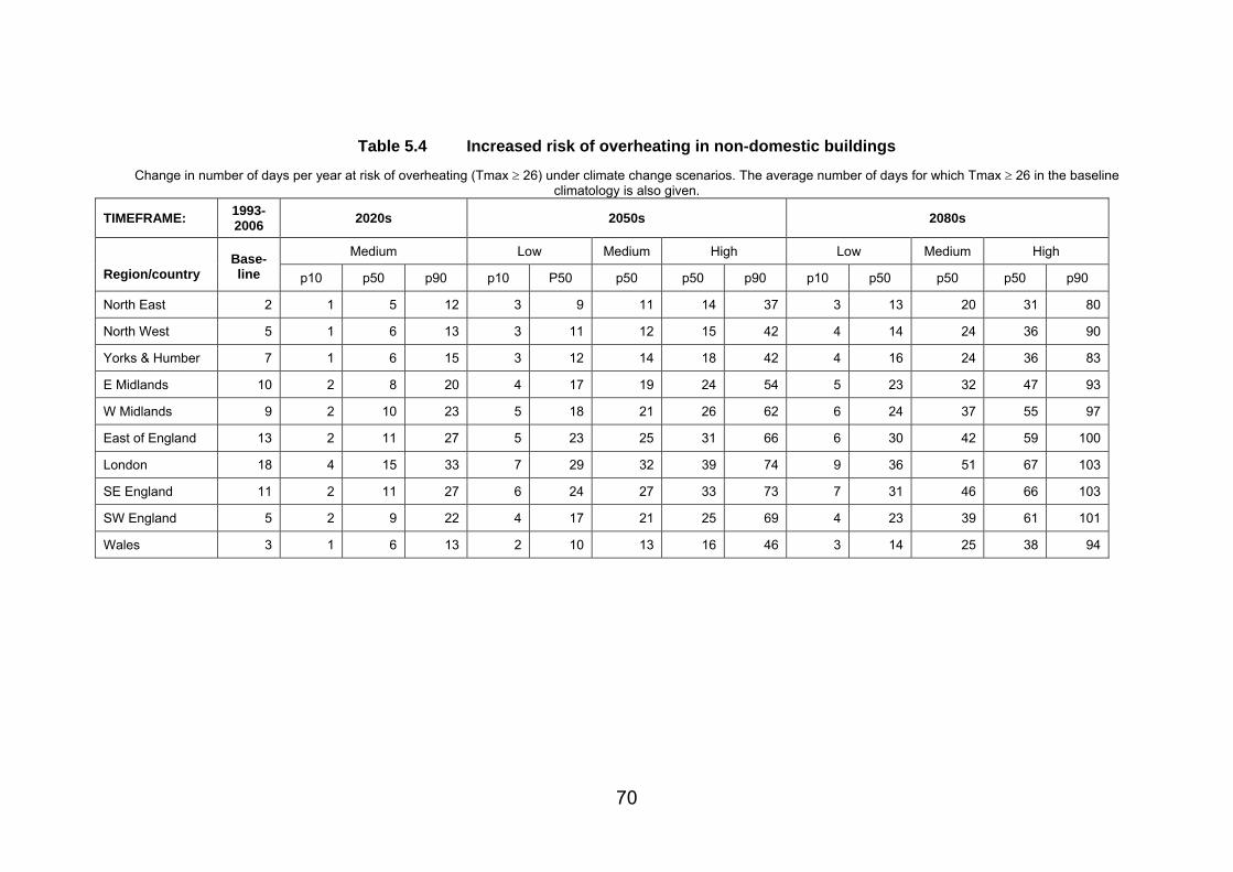
70
Table 5.4 Increased risk of overheating in non-domestic buildings
Change in number of days per year at risk of overheating (Tmax 26) under climate change scenarios. The average number of days for which Tmax 26 in the baseline climatology is also given.
TIMEFRAME: 1993-2006
2020s 2050s 2080s
Medium Low Medium High Low Medium High
Region/country Base-line p10 p50 p90 p10 P50 p50 p50 p90 p10 p50 p50 p50 p90
North East 2 1 5 12 3 9 11 14 37 3 13 20 31 80
North West 5 1 6 13 3 11 12 15 42 4 14 24 36 90
Yorks & Humber 7 1 6 15 3 12 14 18 42 4 16 24 36 83
E Midlands 10 2 8 20 4 17 19 24 54 5 23 32 47 93
W Midlands 9 2 10 23 5 18 21 26 62 6 24 37 55 97
East of England 13 2 11 27 5 23 25 31 66 6 30 42 59 100
London 18 4 15 33 7 29 32 39 74 9 36 51 67 103
SE England 11 2 11 27 6 24 27 33 73 7 31 46 66 103
SW England 5 2 9 22 4 17 21 25 69 4 23 39 61 101
Wales 3 1 6 13 2 10 13 16 46 3 14 25 38 94

Built Environment sector 71
5.7 BE5 – Effectiveness of green space
Summary Class
2020s 2050s 2080s Metric code
Metric name
Co
nfi
den
ce
l c u l c u l c u
BE5 Effectiveness of green space M 1 1 2 1 2 3 2 3 3
The relationship between effective green space and relative aridity developed as a response function was presented in Figure 4.6. A relative aridity score of less than 1 suggests little change in baseline conditions; it is therefore assumed that this has little effect on the cooling capacity of urban green space. A relative aridity score of between 1 and 2 suggests more arid conditions in comparison with the baseline period; a score of greater than 2 suggests extremely arid conditions in comparison with the baseline period.
The impact of relative aridity on the effective area of urban green space in England under the climate change scenarios considered here is summarised in Table 5.5. This implies that a loss of approximately 30% of effective green space by the 2080s (p50 Medium emissions scenario) might occur as an average across England. The range of projections by the 2080s is from 2% to over 70%.
Table 5.5 Reduction in effective green space (Percentage change in total area)
2020s 2050s 2080s
Med
ium
Med
ium
Med
ium
Lo
w
Lo
w
Med
ium
Hig
h
Hig
h
Lo
w
Lo
w
Med
ium
Hig
h
Hig
h
2008 baseline p10 p50 p90 p10 p50 p50 p50 p90 p10 p50 p50 p50 p90
0.0 0.0 0.6 12.2 0.0 11.8 16.4 20.6 39.6 2.2 19.2 30.8 42.8 71.6
It has to be noted that this metric provides only a very general guide to the connection between the reduced effectiveness of urban green space and more prolonged dry, warm periods. It cannot take account of urban microclimates and thus does not account for any UHI effects, for example.
Clearly the nature of urban green space has a major bearing on the cooling capacity it provides; for example the moisture released during transpiration from trees can assist a reduction in air-conditioning requirements within a given building. The value of such space in terms of its amenity, recreation and health benefits is widely acknowledged. Its cooling value is also recognised within heat wave planning; The Heatwave Plan for England (DoH 2010) makes several specific recommendations regarding the use of green space.
The value of green space cooling in terms of reducing localised urban heating effects has been demonstrated (see Section 5.4). Clearly a reduction in cooling capacity due to changes in relative aridity would reduce the capacity of local environments to minimise UHI effects. Conversely the benefits of the green space can be maximised by suitable choice of trees and vegetation and effective management in terms of general husbandry and scheduled watering regimes. In the case of trees, it may take decades for them to come to maturity and provide a shading benefit. Replacement therefore needs to be carefully managed if the overall cooling capacity is not to be compromised. ‘Right tree, right place’ principles should be followed for all green infrastructure (Greater London Authority, 2010a, 2010b).

72 Built Environment sector
Recent research for Defra and DCLG identified several knowledge gaps in this area (Forest Research, 2010). More detailed, statistically valid experimentation is necessary to improve understanding of the mechanisms by which vegetation cools the surrounding environment (Bowler et al., 2010). More information is also needed on suitable species for use in climate change adapted green infrastructure and their physiological characteristics, such as heat and drought tolerance and resistance to frost damage.
While increasing population in urban areas may put pressure on existing green space in terms of a change in land use, increasing population in itself is not a driver of effectiveness of the green space to provide local cooling. This would also be true of changes in the number of domestic or non-domestic buildings within urban areas.
5.8 BE9 – Demand for heating
Summary Class
2020s 2050s 2080s Metric code
Metric name C
on
fid
ence
l c u l c u l c u
BE9 Demand for heating L 1 2 3 2 3 3 2 3 3
5.8.1 Heating Degree Days and Domestic Energy Demand
The projected change in heating degree days for each region has been calculated using UKCP09 projections of changes in mean temperature. The response function developed in Section 4.6 has then been used to calculate the change in domestic space heating demand by region. Background information on the response function is given in Appendix 4 and detailed results are given in Appendix 5.
Broadly speaking there is a reduction in space heating demand in each region, directly correlated with increasing average temperatures. For the purposes of illustration, space heating demand projections under the p50 Medium emissions scenario are shown in Figure 5.3.
-
5,000
10,000
15,000
20,000
25,000
30,000
35,000
40,000
45,000
2008 2010-39 2040-69 2070-99
An
nu
al D
om
es
tic
Sp
ac
e H
ea
tin
g
Co
ns
um
pti
on
(G
Wh
/yr)
East MidlandsEast of EnglandLondonNorth EastNorth WestSouth EastSouth WestWest MidlandsYorkshire and The HumberWalesEast ScotlandNorth ScotlandWest Scotland
Figure 5.3 Projected Domestic Space Heating Energy Consumption (p50 Medium emissions scenario)

Built Environment sector 73
There is a clear reduction in the projected levels of energy demand to heat homes across all regions in future decades. In the case of domestic properties, a continued focus on improvements to roof and cavity wall insulation in existing stock would provide further benefits in reducing space heating demand. Nonetheless, care must be taken that, in implementing such measures, the risk of summer overheating is not increased.
In terms of fuel poverty measures, present metrics focussed on winter heating demands may need to be revised to consider cooling demands as well. This may be especially true for the elderly in providing assistance in summer heat events as well as in supporting energy efficiency programmes to reduce fuel costs in winter.
5.8.2 DECC 2050 Pathways
The DECC 2050 Pathways Report also provides trajectories for future heating demand (DECC 2010c). These include both climate and non-climate drivers. They are included here in order to provide a qualitative illustration of possible future demand.
Figure 5.4 shows trajectories for domestic space heating and hot water energy demand. Level 1 includes increased user demand in terms of internal temperatures and hot water use, but also some increase in domestic energy efficiency. At Level 4, consumer demand is significantly reduced and energy efficiency significantly increased.
Figure 5.4 DECC 2050 Pathways trajectories for heating (space and hot water) demand for domestic sector
Source: DECC (2010c)
Figure 5.5 shows similar trajectories for the non-domestic sector. In all scenarios shown the number of buildings increases by 1% per annum. At Level 1 there is little change either in user demand or building regulation requirements for energy efficiency. Level 4 includes considerable reductions in demands for space heating (90% in new build, 40% in old build) and hot water (30%) driven by widespread increases in energy efficiency, achieved by refurbishment of old buildings and improved new-build standards. The results indicate the magnitude of increase that might occur with no adaptation actions (Level 1).

74 Built Environment sector
Figure 5.5 DECC 2050 Pathways trajectories for heating (space and hot water) demand for non-domestic sector
Source: DECC (2010c)
5.9 EN2 – Energy demand for cooling
Summary Class
2020s 2050s 2080s Metric code
Metric name
Co
nfi
den
ce
l c u l c u l c u
EN2 Energy demand for cooling H 2 2 2 2 2 3 2 3 3
Two approaches are used to assess cooling demand, cooling degree days and the DECC pathway analysis. Further details of the methods and results are provided in the Energy sector report (McColl et al., 2012).
5.9.1 Cooling degree days
An estimate has been made of projections of cooling degree days (CDD) as an indicator of how the burden of cooling demand may change in the future as a result of climate factors only.
The ensemble mean simulation of CDD for 1961-1990, and the mean changes in CDD for the three future periods 2020s, 2050s and 2080s, are shown in Figure 5.6 (top row), together with the model range within the ensemble (bottom row). These results show that the CDD are projected to increase significantly during the twenty-first century, especially over southern England. The average CDD over southern England for the1961-1990 ensemble mean are simulated to be approximately 25 to 50, whereas by the 2080s they have increased to between 125 and 175.
The projected increase in CDD is reduced with increasing latitude, such that the increases over northern England and Scotland are much smaller (25 to 50). The variation between the projected changes in CDD also increases during the 21st century; the largest uncertainties are in the same locations as the largest increases in CDD.

Built Environment sector 75
From the projections of future CDD, it is possible to infer that cooling demand may increase in the future as a consequence of increasing temperatures. However it is important to consider these projections relative to current conditions since demand associated with cooling is currently small compared to heating. It could therefore be inferred that the increase in cooling demand based on climate factors alone could be met with the current capacity of the electricity network (particularly as the requirement for heating may reduce).
The future requirements for cooling will be affected by a number of factors including wealth (and affordability) and mitigation policies, for example measures to improve the efficiency of the UK housing stock are likely to change the thermal properties of UK houses.
5.9.2 DECC 2050 Pathways and other analysis
The objective of the second part of this analysis is to understand how a change in cooling requirements will impact on energy demand. Although there are not sufficient data available to carry out a quantitative analysis, there are projections of cooling demand available from Day et al. (2009) and DECC’s 2050 Pathway Analysis (DECC, 2010c). These are used to assess qualitatively the impact of climate change on cooling demand, as measured in terms of energy increases.
The analysis by Day et al. (2009) examines changes to building stock, air-conditioning and climate affected energy demand projections for London up to 2030, varying only the climate change scenarios (no, low and high climate scenarios). Under a high climate scenario, cooling energy demand is projected to rise from approximately 1.6TWh in 2004 to 2.5TWh (50% increase) and under a low climate scenario it is projected to rise from approximately 1.6TWh to 2.2TWh (35% increase).
Since the Day et al. (2009) study focussed on London, trajectories for UK future cooling demand from the 2050s Pathway Analysis are also presented here. The trajectories are provided for four different levels for both domestic and non-domestic sectors; they are illustrated in Figure 5.7. The domestic trajectories range from no additional domestic air conditioning (Level 4) to all houses installing an air conditioning system (Level 1).
This results in a potential rise from 0 in 2007 to 50 TWh per year by the 2050s for domestic cooling demand. It is stressed that these increases are primarily a response to increased wealth, although they do factor in future external temperature and climate change23. They therefore reflect the total change, i.e. the combined effects of socio-economic and climate change together, rather than the marginal change due to climate alone.
The non-domestic trajectories illustrate a range of scenarios including different uptakes of air-conditioning and efficiencies in existing systems. At best, there is a reduction of about 50% compared to 2007 levels due to an increased use of passive air conditioning (Level 4) and at worst an increase of approximately 300% if all non-domestic floor space install air-conditioning systems (Level 1).
23 The figures include growth in dwelling numbers, the change in average dwelling heat loss, projected changes in external temperature and the effect of changes to internal gains from hot water heating, lights and appliances. A cooling set point at an internal temperature of 23.5°C has been assumed.
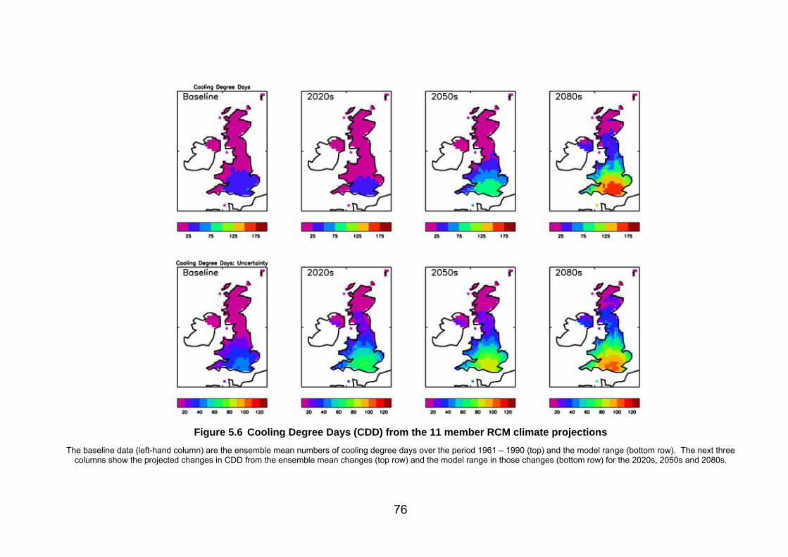
76
Figure 5.6 Cooling Degree Days (CDD) from the 11 member RCM climate projections
The baseline data (left-hand column) are the ensemble mean numbers of cooling degree days over the period 1961 – 1990 (top) and the model range (bottom row). The next three columns show the projected changes in CDD from the ensemble mean changes (top row) and the model range in those changes (bottom row) for the 2020s, 2050s and 2080s.

Built Environment sector 77
Figure 5.7 Trajectories for domestic (top) and non-domestic (bottom) cooling demand
Source: DECC (2010c)
5.10 WA5 – Water supply-demand deficit Summary Class
2020s 2050s 2080s Metric code
Metric name
Co
nfi
den
ce
l c u l c u l c u
WA5 Water supply-demand deficit M 1 1 2 1 3 3 2 3 3 Key considerations for these calculations include assumptions made in the analysis about headroom, which is the component used to manage uncertainties in the water supply-demand balance, leakage, which is a significant component of the balance in many parts of the UK, and the current baseline surplus or deficit that exists for each UKCP09 river basin region.
In this assessment the future percentage headroom is the same as in the base year. This ensures a consistent approach across the UK but underestimates this component compared to what is reported in water company plans: Headroom generally increases

78 Built Environment sector
through time as the future is more uncertain than the present. Similarly, leakage has not been considered in detail although this may be sensitive to climate, for example cold winters may increase the frequency of pipe bursts, while warmer winters may lead to fewer pipe bursts. Further detailed studies on climate and leakage are planned in 2011/12 and this element may be assessed in future cycles of the CCRA.
If supply versus demand as a simple balance of water available for use is considered, comprising imports and exports and ‘distribution input’ (without maintaining any additional allowance for uncertainties), most parts of the UK currently have sufficient public water supplies and some, such as the North East, have large surpluses of available water. This is reflected in assessments in England and Wales that show a high security of supply in most water resources zones, with some risks highlighted for zones in the South East, South West, Midlands and North Wales (Environment Agency, 2008 based on Ofwat data). If the UK is considered as a whole and it is assumed that water is transferred between companies, then the current balance is very healthy and there is a projected surplus of around 237 Ml/d (ranging from a surplus of 2280 Ml/d to a deficit of 2040 Ml/d) by the 2020s.
However, major water transfers are very expensive, have high energy costs for pumping water and also some environmental constraints. Companies also need to retain some additional resources (typically 5 to 10%) in order to deal with uncertainties in their supply-demand calculations. If it is assumed that companies are unable to share resources then impacts could be much higher, with a projected deficit of around 377 Ml/d (0 to -2281 Ml/d) by the 2020s. Currently the situation is closer to the latter case as the costs of major transfers are deemed far greater than those of local resource development, demand management and even desalinisation.
It should be noted that there are limitations involved in summing regional results to get a national figure, particularly for more extreme scenarios. For this reason the water balance results are most appropriately used at the scale of UKCP09 river basin regions rather than averaging data up to the country or UK scale. Figure 5.8 shows the results for this metric assuming no sharing of water across regions. The full results for WA5, including the current surplus/deficit and detailed changes assuming sharing of water across regions for each UKCP09 basin, can be found in the Water sector report (Rance et al., 2012).

Built Environment sector 79
Figure 5.8 The water supply-demand balance assuming no sharing of water across regions
Projections are shown by UKCP09 river basin region (Ml/d)
The maps in Figure 5.8 show the range of deficits across each UKCP09 river basin region. The largest deficits are projected to occur in the Thames river basin region, with a deficit of around 955 Ml/d (range -47 to -1780 Ml/d) by the 2050s that increases to a deficit of 1340 Ml/d (range -277 to -1840 Ml/d) by the 2080s. A number of river basin regions are projected to experience no deficit in supplies for some scenarios, including Neagh Bann, Tweed and Forth. One basin, North East Scotland, is projected to experience no deficit in supplies for all scenarios. These results indicate the wide regional variations in the results.

80 Built Environment sector
5.11 WA6 – Population affected by a water supply-demand deficit
Summary Class
2020s 2050s 2080s Metric code
Metric name
Co
nfi
den
ce
l c u l c u l c u
WA6 Population affected by a water supply-demand deficit M 1 2 2 1 2 2 2 2 3
The projected impacts of climate change on the population affected by a supply-demand deficit (when water resource zones fall into deficit and require demand or supply side measures) are summarised in Figure 5.9. Full results for this metric are given in the Water sector report. The results of the analysis indicate that between 15% and 80% of the population could be affected by a water-supply demand deficit by the 2020s, rising to between 65% and over 95% by the 2080s (based on Table A7.10 in Rance et al., 2012).
By looking at the data by UKCP09 river basin region, it is apparent that although this could be an issue for much of the country, there are variations. This would determine whether intervention would be required at the national or local level. For example, (looking at detailed figures) while almost all of the population for the Thames, Neagh Bann and Western Wales basins is projected to be affected by supply-demand deficits by the 2080s, other river basin regions such as Clyde and North West England are less affected.
As well as households, public services such as schools and hospitals are large users of water from both public water supply and their own groundwater abstraction licences24. Any disruption of supply for these essential services would have significant consequences and maintaining these supplies is a priority in water company drought plans and emergency plans.
There are specific concerns about vulnerable groups and the affordability of water in England and Wales that were considered as part of the Walker Review (2009). Tackling affordability issues is a key theme in the Water White Paper, Water for Life, published in December 2011. At present, water utility bills are highest in the south west. The Water White Paper addressed this by committing Government to discounting customer bills in the south west by £50 per annum (Defra (2011). In Northern Ireland they have traditionally been included in rates, rather than as a separate tariff.
It should be noted that these figures show the population affected by a supply-demand deficit assuming that no intervention takes place. In reality however, water companies do account for these projected deficits by considering different supply and demand-side management options in their Water Resources Management Plans for the period up to 2035.
24 Data on hospital water use in available http://www.hefs.ic.nhs.uk/

Built Environment sector 81
Figure 5.9 The population affected by a supply-demand deficit due to climate change only
Projections are shown by UKCP09 river basin region

82 Built Environment sector
5.12 FL6, FL7 and FL13 - Flooding of properties
5.12.1 Residential properties at significant likelihood of flooding and EAD (Metric FL6)
Summary Class 2020s 2050s 2080s Metric
code Metric name
Co
nfi
den
ce
l c u l c u l c u
FL6a Residential properties at significant likelihood of flooding
H 2 2 2 2 3 3 2 3 3
FL6b EAD for residential properties (tidal and river)
H 3 3 3 3 3 3 3 3 3
Number of residential properties at significant likelihood of flooding (Metric FL6a)
The number of residential properties at significant likelihood of flooding (i.e. annual probability of flooding of 1.3% or greater) is projected to range from about 500,000 to 800,000 in the 2020s compared with a baseline of about 370,000, rising to between 700,000 and 1.1 million by the 2080s for the range of climate change scenarios used in the analysis.
EAD for residential properties (Metric FL6b)
The Expected Annual Damages for residential properties is projected to range from about £750 million to £1.6 billion in the 2020s compared with a baseline of about £640 million, rising to about £1.1billion to £3.4 billion by the 2080s for the range of climate change scenarios used in the analysis (at present day prices).
These figures cover tidal and river flooding, but not surface water flooding. Further details are given in Section 5.12.3 below.
5.12.2 Non-residential properties at significant likelihood of flooding and EAD (Metric FL7)
Summary Class
2020s 2050s 2080s Metric code
Metric name
Co
nfi
den
ce
l c u l c u l c u
FL7a Number of non-residential properties at significant likelihood of flooding
H 1 3 3 2 3 3 2 3 3
FL7b EAD for non-residential properties (fluvial and tidal)
H 2 3 3 3 3 3 3 3 3
Number of non-residential properties at significant likelihood of flooding (Metric FL7a)
The number of non-residential properties at significant likelihood of flooding is projected to range from about 200,000 to 350,000 in the 2020s compared with the baseline of about 190,000, rising to about 300,000 to 400,000 by the 2080s for the range of climate change scenarios used in the analysis.

Built Environment sector 83
EAD for non-residential properties (Metric FL7b)
The Expected Annual Damages for non-residential properties is projected to range from about £650 million to £1.4 billion in the 2020s compared with a baseline of about £560 million, rising to about £1 billion to £2.7 billion by the 2080s for the range of climate change scenarios used in the analysis (at present day prices).
These figures cover tidal and river flooding, but not surface water flooding. Further details are given in Section 5.12.3 below.
5.12.3 Total numbers of properties and EAD
The number of properties (residential and non-residential) at significant likelihood of flooding is shown on Figure 5.10.
Properties at significant risk of flooding
0
200000
400000
600000
800000
1000000
1200000
1400000
1600000
1 2 3 4 5
Nu
mb
er o
f p
rop
ert
ies
Res - fluvial Non-res - fluvial Res - tidal Non-res tidal Res - total Non-res - total Total
Observed (2008 tidal)
2010-39 2040-69 2070-99Baseline (1961-90 fluvial)
The columns are based on the P50 Medium Emissions climate change scenario.
The arrows indicate the approximate ranges of projections for other climate change scenarios used in the analysis.
Figure 5.10 Number of properties at significant likelihood of flooding
The Expected Annual Damages for properties (residential and non-residential) is shown on Figure 5.11.

84 Built Environment sector
Expected annual damage for all properties
0
1000
2000
3000
4000
5000
6000
7000
1 2 3 4 5
EA
D (
£ m
illio
ns
)
Res - fluvial Non-res - fluvial Res - tidal Non-res - tidal Res - total Non-res - total Overall total
Observed (2008 tidal)
2010-39 2040-69 2070-99Baseline (1961-90 fluvial)
The columns are based on the P50 Medium Emissions climate change scenario.
The arrows indicate the approximate ranges of projections for other climate change scenarios used in the analysis.
Figure 5.11 EAD for properties (residential and non-residential)
The total numbers of properties and EAD are summarised in Table 5.6 for the p50 Medium emissions climate change scenario.
Table 5.6 Total properties and EAD from metrics FL6 and FL7 River and coastal/tidal flooding only
Baseline: 1961-90 (fluvial); 2008 (tidal) p50 Medium emissions climate change scenario
Properties (thousands) EAD (£ millions) Year Res Non-res Total Res Non-res Total
Baseline 370 190 560 640 560 1200 2020s 480 – 820 230 – 340 700 – 1160 750 – 1600 650 – 1400 1400 – 3000 2050s 530 – 1000 230 – 390 760 – 1390 850 – 2500 750 – 2000 1600 – 4500 2080s 700 – 1090 300 – 410 990 – 1500 1150 – 3450 950 – 2700 2100 – 6150
It may be concluded that:
The median projection for the total number of properties at significant likelihood of flooding is an increase to about 1.3 million by the 2080s from a baseline of about 560,000 if the defences are maintained to present crest levels and condition.
The median projection for the Expected Annual Damage to properties from flooding is an increase to over £3.5 billion by the 2080s from a baseline of about £1.2 billion if the defences are maintained to present crest levels and condition.
These figures cover tidal and river flooding, but not surface water flooding.
It is provisionally estimated that there is a total of about 2.8 million properties at risk from river and tidal flooding in the UK. It is also estimated that there are about 4.2
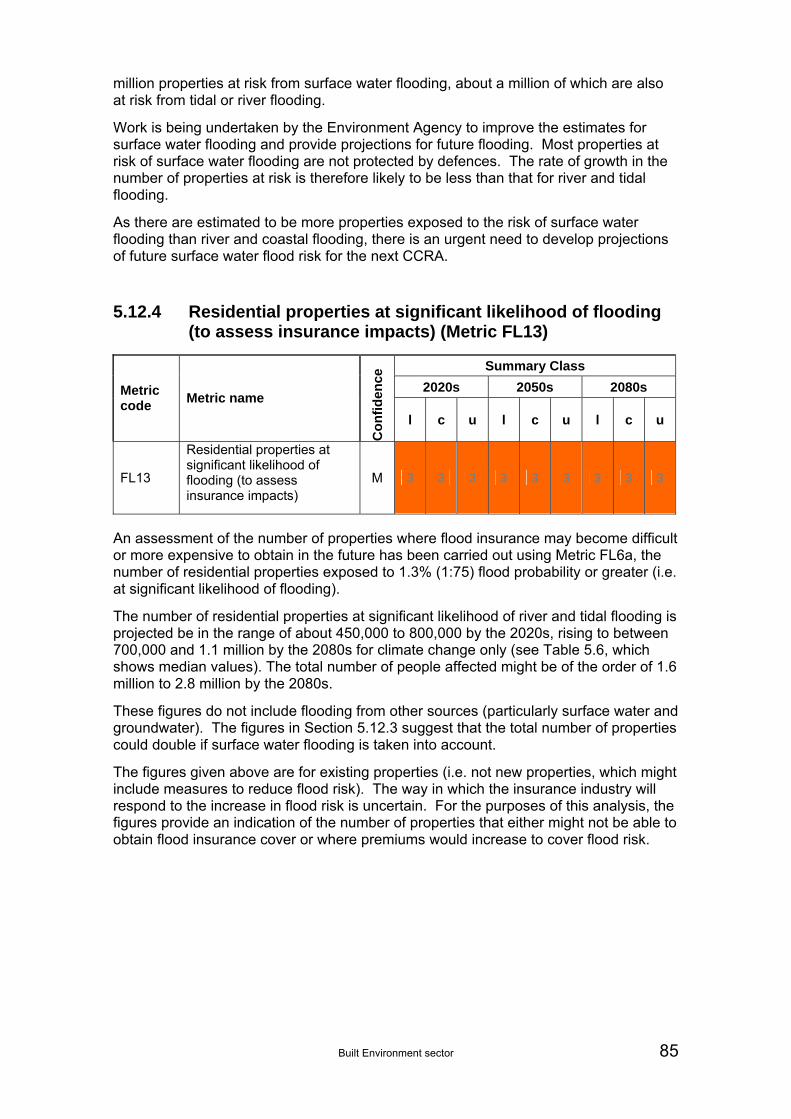
Built Environment sector 85
million properties at risk from surface water flooding, about a million of which are also at risk from tidal or river flooding.
Work is being undertaken by the Environment Agency to improve the estimates for surface water flooding and provide projections for future flooding. Most properties at risk of surface water flooding are not protected by defences. The rate of growth in the number of properties at risk is therefore likely to be less than that for river and tidal flooding.
As there are estimated to be more properties exposed to the risk of surface water flooding than river and coastal flooding, there is an urgent need to develop projections of future surface water flood risk for the next CCRA.
5.12.4 Residential properties at significant likelihood of flooding (to assess insurance impacts) (Metric FL13)
Summary Class
2020s 2050s 2080s Metric code
Metric name
Co
nfi
den
ce
l c u l c u l c u
FL13
Residential properties at significant likelihood of flooding (to assess insurance impacts)
M 3 3 3 3 3 3 3 3 3
An assessment of the number of properties where flood insurance may become difficult or more expensive to obtain in the future has been carried out using Metric FL6a, the number of residential properties exposed to 1.3% (1:75) flood probability or greater (i.e. at significant likelihood of flooding).
The number of residential properties at significant likelihood of river and tidal flooding is projected be in the range of about 450,000 to 800,000 by the 2020s, rising to between 700,000 and 1.1 million by the 2080s for climate change only (see Table 5.6, which shows median values). The total number of people affected might be of the order of 1.6 million to 2.8 million by the 2080s.
These figures do not include flooding from other sources (particularly surface water and groundwater). The figures in Section 5.12.3 suggest that the total number of properties could double if surface water flooding is taken into account.
The figures given above are for existing properties (i.e. not new properties, which might include measures to reduce flood risk). The way in which the insurance industry will respond to the increase in flood risk is uncertain. For the purposes of this analysis, the figures provide an indication of the number of properties that either might not be able to obtain flood insurance cover or where premiums would increase to cover flood risk.
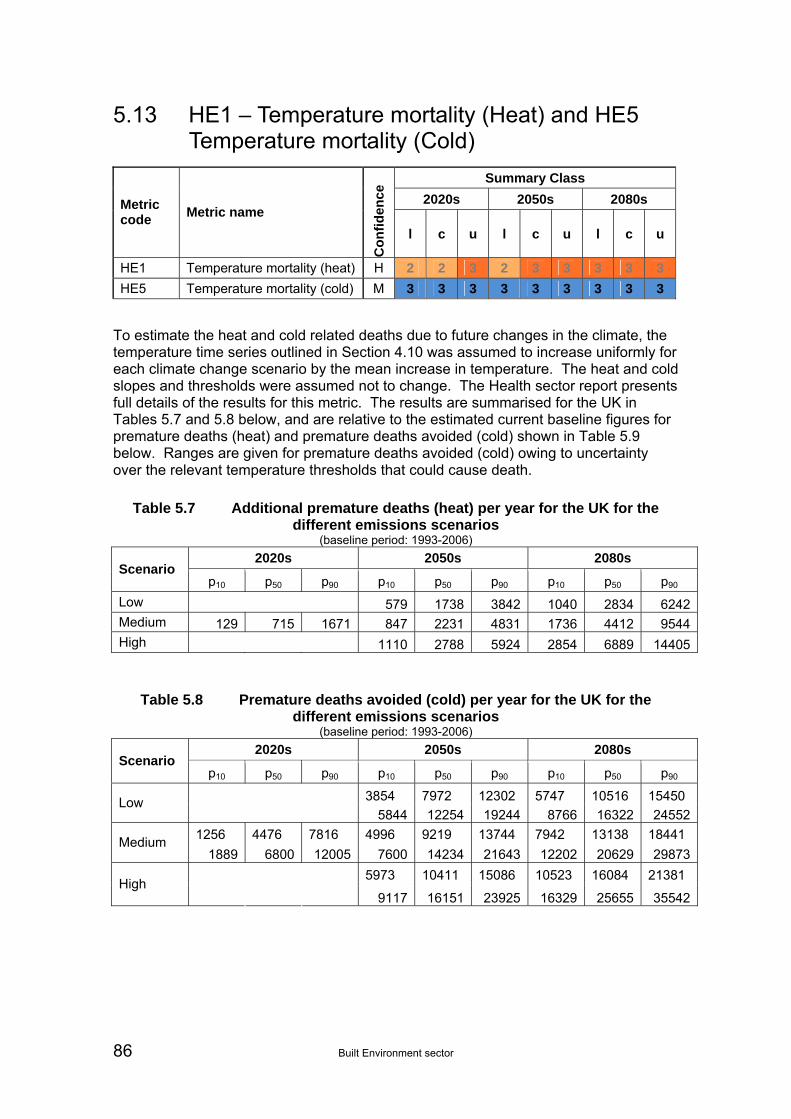
86 Built Environment sector
5.13 HE1 – Temperature mortality (Heat) and HE5 Temperature mortality (Cold)
Summary Class
2020s 2050s 2080s Metric code
Metric name
Co
nfi
den
ce
l c u l c u l c u
HE1 Temperature mortality (heat) H 2 2 3 2 3 3 3 3 3
HE5 Temperature mortality (cold) M 3 3 3 3 3 3 3 3 3
To estimate the heat and cold related deaths due to future changes in the climate, the temperature time series outlined in Section 4.10 was assumed to increase uniformly for each climate change scenario by the mean increase in temperature. The heat and cold slopes and thresholds were assumed not to change. The Health sector report presents full details of the results for this metric. The results are summarised for the UK in Tables 5.7 and 5.8 below, and are relative to the estimated current baseline figures for premature deaths (heat) and premature deaths avoided (cold) shown in Table 5.9 below. Ranges are given for premature deaths avoided (cold) owing to uncertainty over the relevant temperature thresholds that could cause death.
Table 5.7 Additional premature deaths (heat) per year for the UK for the different emissions scenarios
(baseline period: 1993-2006)
2020s 2050s 2080s Scenario
p10 p50 p90 p10 p50 p90 p10 p50 p90
Low 579 1738 3842 1040 2834 6242Medium 129 715 1671 847 2231 4831 1736 4412 9544High 1110 2788 5924 2854 6889 14405
Table 5.8 Premature deaths avoided (cold) per year for the UK for the different emissions scenarios
(baseline period: 1993-2006)
2020s 2050s 2080s Scenario
p10 p50 p90 p10 p50 p90 p10 p50 p90
3854 7972 12302 5747 10516 15450 Low 5844 12254 19244 8766 16322 24552
1256 4476 7816 4996 9219 13744 7942 13138 18441 Medium
1889 6800 12005 7600 14234 21643 12202 20629 29873
5973 10411 15086 10523 16084 21381 High
9117 16151 23925 16329 25655 35542
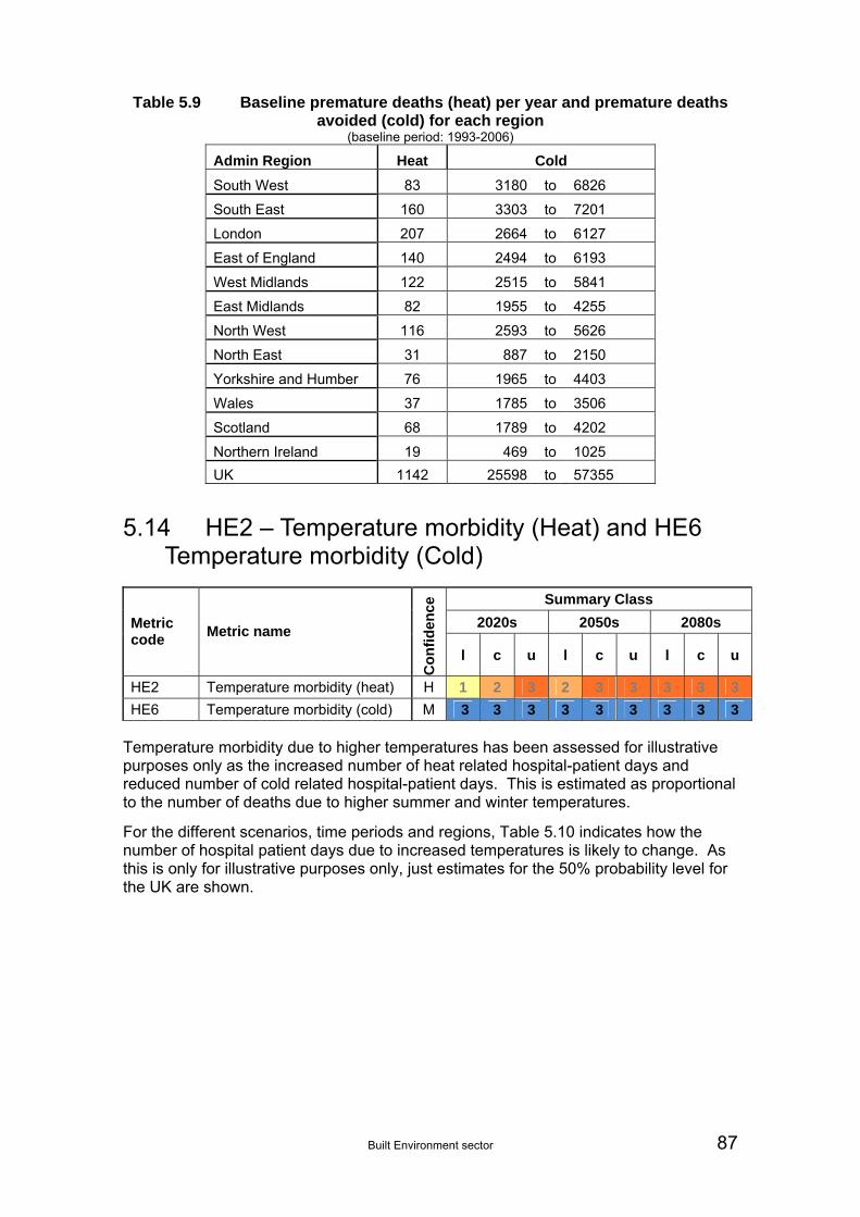
Built Environment sector 87
Table 5.9 Baseline premature deaths (heat) per year and premature deaths avoided (cold) for each region
(baseline period: 1993-2006)
Admin Region Heat Cold
South West 83 3180 to 6826
South East 160 3303 to 7201
London 207 2664 to 6127
East of England 140 2494 to 6193
West Midlands 122 2515 to 5841
East Midlands 82 1955 to 4255
North West 116 2593 to 5626
North East 31 887 to 2150
Yorkshire and Humber 76 1965 to 4403
Wales 37 1785 to 3506
Scotland 68 1789 to 4202
Northern Ireland 19 469 to 1025
UK 1142 25598 to 57355
5.14 HE2 – Temperature morbidity (Heat) and HE6 Temperature morbidity (Cold)
Summary Class
2020s 2050s 2080s Metric code
Metric name
Co
nfi
den
ce
l c u l c u l c u
HE2 Temperature morbidity (heat) H 1 2 3 2 3 3 3 3 3
HE6 Temperature morbidity (cold) M 3 3 3 3 3 3 3 3 3 Temperature morbidity due to higher temperatures has been assessed for illustrative purposes only as the increased number of heat related hospital-patient days and reduced number of cold related hospital-patient days. This is estimated as proportional to the number of deaths due to higher summer and winter temperatures.
For the different scenarios, time periods and regions, Table 5.10 indicates how the number of hospital patient days due to increased temperatures is likely to change. As this is only for illustrative purposes only, just estimates for the 50% probability level for the UK are shown.

88 Built Environment sector
Table 5.10 Annual additional patient days due to increased high temperatures and annual patient days avoided due to increased low
temperatures (both thousands, p50) – tentative estimates (baseline period: 1993-2006)
Low emissions Medium emissions High emissions UK only
2050s 2080s 2020s 2050s 2080s 2050s 2080sHeat: additional patient days 177 289 73 228 450 284 703
813 1073 457 940 1340 1062 1641 Cold: reduction in patient days, lower and upper bounds 1250 1665 694 1452 2104 1647 2617
5.15 HE3 – Flood related deaths
Summary Class
2020s 2050s 2080s Metric code
Metric name
Co
nfi
den
ce
l c u l c u l c u
HE3 Flood related deaths H 1 2 2 2 2 2 2 2 2
Flood related deaths as a result of a changing climate are assumed to be proportional to the number of people at risk due to fluvial or tidal flooding. For overtopping of seawalls, flood related deaths are assumed to increase exponentially in relation to changes in mean sea levels. Changes in deaths due to storms are assumed to be negligible. Baseline rates for deaths due to extreme event flooding and storms are assumed to be 18 per year (Section 4.12).
For the different scenarios, time periods and probability bands considered, Table 5.11 gives the estimated number of deaths due to future extreme event flooding and storms.
Table 5.11 Annual additional flood related deaths due to extreme event flooding and storms25
2020s 2050s 2080s Med Med Med Low Low Med High High Low Low Med High HighScenario
p10 p50 p90 p10 p50 p50 p50 p90 p10 p50 p50 p50 p90 Total (present day demographics)
22 30 35 24 36 39 42 52 31 44 49 57 87
Climate change effect
4 12 17 6 18 21 24 34 13 26 31 39 69
25 The climate change effect is those deaths from the total that are attributed to climate change. The difference between the figures is the current day baseline estimate of 22 deaths per year.
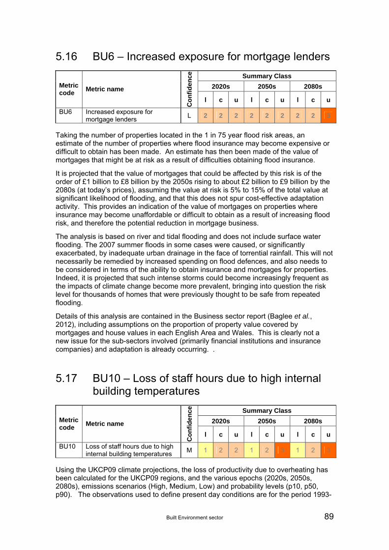
Built Environment sector 89
5.16 BU6 – Increased exposure for mortgage lenders
Summary Class
2020s 2050s 2080s Metric code
Metric name
Co
nfi
den
ce
l c u l c u l c u
BU6 Increased exposure for mortgage lenders
L 2 2 2 2 2 2 2 2 3
Taking the number of properties located in the 1 in 75 year flood risk areas, an estimate of the number of properties where flood insurance may become expensive or difficult to obtain has been made. An estimate has then been made of the value of mortgages that might be at risk as a result of difficulties obtaining flood insurance.
It is projected that the value of mortgages that could be affected by this risk is of the order of £1 billion to £8 billion by the 2050s rising to about £2 billion to £9 billion by the 2080s (at today’s prices), assuming the value at risk is 5% to 15% of the total value at significant likelihood of flooding, and that this does not spur cost-effective adaptation activity. This provides an indication of the value of mortgages on properties where insurance may become unaffordable or difficult to obtain as a result of increasing flood risk, and therefore the potential reduction in mortgage business.
The analysis is based on river and tidal flooding and does not include surface water flooding. The 2007 summer floods in some cases were caused, or significantly exacerbated, by inadequate urban drainage in the face of torrential rainfall. This will not necessarily be remedied by increased spending on flood defences, and also needs to be considered in terms of the ability to obtain insurance and mortgages for properties. Indeed, it is projected that such intense storms could become increasingly frequent as the impacts of climate change become more prevalent, bringing into question the risk level for thousands of homes that were previously thought to be safe from repeated flooding.
Details of this analysis are contained in the Business sector report (Baglee et al., 2012), including assumptions on the proportion of property value covered by mortgages and house values in each English Area and Wales. This is clearly not a new issue for the sub-sectors involved (primarily financial institutions and insurance companies) and adaptation is already occurring. .
5.17 BU10 – Loss of staff hours due to high internal building temperatures
Summary Class
2020s 2050s 2080s Metric code
Metric name
Co
nfi
den
ce
l c u l c u l c u
BU10 Loss of staff hours due to high internal building temperatures
M 1 2 2 1 2 3 1 2 3
Using the UKCP09 climate projections, the loss of productivity due to overheating has been calculated for the UKCP09 regions, and the various epochs (2020s, 2050s, 2080s), emissions scenarios (High, Medium, Low) and probability levels (p10, p50, p90). The observations used to define present day conditions are for the period 1993-

90 Built Environment sector
2006. However, the changes used to make the climate change projections all relate to the period 1961-90 as a baseline.
Given that the first projection epoch is for the interval 2010-2039 (labelled 2020s) it can be argued that the observed data should already include some of the projected change. However, determining how much change to assign depends on the degree to which a trend can be detected in the observations and the extent to which any such trend can be attributed to climate change.
In the case of temperature it is considered that changes since the baseline period of 1961-90 can be identified and attributed to climate change. Temperature records suggest that the period post-1990 is of the order of 0.5C warmer. The observed period could, therefore, already include about half of the change projected to the first epoch (2020s). The UKCP09 temperature variables, used to scale Tmax and Tmean, were therefore adjusted by this amount for all epochs.
The results using a 26C threshold are presented in Table 5.12 and those for a 28C threshold in Table 5.13. The values obtained suggest as much as a doubling in lost productivity as an upper bound by 2020s (p90 values), with little change at the lower bound (p10 values). By the 2050s the central estimate is for a 3-fold increase, on average, increasing to an average increase of 8-9 times for the high emissions, p90 case. This pattern continues into the 2080s, with roughly a 50% increase in lost productivity for the p10 case, and an increase of anything from 10-50 times for the high emissions, p90 case. If the climate change projections were simply added to the observed values, without the adjustment to baseline described above, these values would be further increased by about 50-80% in the near-term, and some 40-50% for the 2080s.
Table 5.12 Lost production days per year per employee for days exceeding 26C
Includes an adjustment to take account of the underlying changes since the time of the baseline period (1961-90)
2020s 2050s 2080s Medium Medium Medium Low Medium High Low Medium High
Region Baseline p10 p50 p90 p10 p50 p90 p10 p50 p90
East Midlands 0.25 0.29 0.37 0.49 0.36 0.64 1.55 0.37 1.09 4.36
East of England 0.33 0.36 0.47 0.65 0.47 0.87 2.08 0.48 1.44 5.50
London 0.53 0.58 0.77 1.03 0.74 1.33 3.05 0.77 2.14 7.47
North East 0.05 0.05 0.09 0.15 0.08 0.21 0.63 0.08 0.43 2.39
North West 0.13 0.15 0.21 0.30 0.20 0.38 0.97 0.20 0.67 3.14
South East 0.27 0.31 0.43 0.61 0.41 0.83 2.21 0.43 1.45 6.25
South West 0.11 0.12 0.20 0.32 0.19 0.46 1.51 0.20 0.92 5.35
West Midlands 0.25 0.28 0.38 0.55 0.36 0.71 1.75 0.39 1.21 5.22 Yorkshire & Humberside
0.16 0.18 0.25 0.33 0.24 0.42 1.05 0.25 0.72 3.05
Wales 0.08 0.09 0.13 0.21 0.12 0.29 0.89 0.13 0.59 3.47

Built Environment sector 91
Table 5.13 Lost production days per year per employee for days exceeding 28C
Includes an adjustment to take account of the underlying changes since the time of the baseline period (1961-90)
2020s 2050s 2080s Medium Medium Medium Low Medium High Low Medium High
Region Baseline p10 p50 p90 p10 p50 p90 p10 p50 p90
East Midlands 0.15 0.17 0.24 0.33 0.23 0.44 1.14 0.24 0.73 3.66
East of England 0.18 0.21 0.31 0.43 0.30 0.57 1.55 0.31 1.00 4.79
London 0.36 0.39 0.54 0.72 0.51 0.98 2.46 0.54 1.64 6.73
North East 0.01 0.02 0.03 0.06 0.02 0.09 0.37 0.02 0.23 1.75
North West 0.08 0.09 0.13 0.18 0.12 0.23 0.67 0.12 0.45 2.35
South East 0.15 0.18 0.25 0.39 0.25 0.53 1.61 0.26 1.00 5.51
South West 0.06 0.07 0.10 0.16 0.09 0.26 0.99 0.10 0.56 4.56
West Midlands 0.14 0.17 0.24 0.35 0.23 0.48 1.29 0.25 0.86 4.50 Yorkshire & Humberside
0.07 0.08 0.12 0.19 0.12 0.26 0.69 0.13 0.47 2.39
Wales 0.04 0.05 0.08 0.12 0.07 0.15 0.54 0.08 0.34 2.59
Although the approach involves a number of assumptions it does provide an initial indication of the order of magnitude of this consequence. There is also anecdotal evidence that there is increased absenteeism during warm periods. The above estimates do not include this effect.
Exposure of Sections and Divisions of Industries
The Business sector report contains analysis of the impact of this reduction in productivity on different sectors of business, industry and services. Table 5.14 summarises these results.
Table 5.14 Staff days lost and indicative cost using thresholds of 26C and 28C
2020s 2050s 2080s Medium Medium Medium Low Medium High Low Medium High
Tmax >26C Baseline p10 p50 p90 p10 p50 p90 p10 p50 p90 Staff days lost (x1000)
5120 5690 7770 10750 7430 14170 35680 7780 24290 101330
% of working time 0.10% 0.11% 0.16% 0.21% 0.15% 0.28% 0.71% 0.16% 0.49% 2.02%
Cost (£m) 770 850 1170 1610 1120 2130 5350 1170 3640 15200 % of turnover 0.02% 0.02% 0.03% 0.04% 0.03% 0.06% 0.14% 0.03% 0.10% 0.41%
Tmax >28C Staff days lost (x1000)
3050 3480 4890 6970 4650 9490 26270 4920 17010 86610
% of working time 0.06% 0.07% 0.10% 0.14% 0.09% 0.19% 0.52% 0.10% 0.34% 1.73%
Cost (£m) 460 520 730 1050 700 1420 3940 740 2550 12990 % of turnover 0.01% 0.01% 0.01% 0.02% 0.01% 0.03% 0.08% 0.01% 0.05% 0.25%
Ratio of costs 1.68 1.64 1.59 1.54 1.60 1.49 1.36 1.58 1.43 1.17
Conclusions
A number of assumptions have had to be made to get an estimate of how increased temperatures, notably during the summer months, are likely to affect worker productivity. The confidence in some of these assumptions or sources is generally low and hence the confidence in the overall estimates is low. However, they do serve to indicate that this could be a serious consequence with the potential to increase business costs substantially, unless suitable adaptation measures are introduced.

92 Built Environment sector
6 Socio-economic Changes
6.1 Introduction
In examining the socio-economic impacts on the estimated changes in the metrics outlined in Chapter 5, regional population and household projections (consistent with present DCLG estimates), to the 2050s, have been used. Three projections (low, principal and high) have been used in presenting possible socio-economic change.
In trying to quantify potential socio-economic drivers for the 2080s, which may influence the metrics identified in this study, three sets of socio-economic dimensions (listed below) have been devised following consultation with sector analysts and project team members. These dimensions represent socio-economic drivers that may have the potential to make a significant impact on the particular sector risks identified, but also contain a high degree of uncertainty making them unsuitable to model as a forecast.
Population needs/demands (high/low)
This dimension is intended to encapsulate drivers of population size and distribution (geographically and demographically) and the pressure the population forces onto the country in terms of housing, education etc. One extreme is that there is a high degree of demand on natural, economic and social resources (demand exceeds supply and more people are exposed to risk); the other is that demand is very low (supply exceeds demand and people are less exposed to risk).
Distribution of wealth (even/uneven)
This dimension considers the distribution of wealth amongst the British population; the extremes being whether it is more even compared to today or more uneven (with a strong gradient between the rich and poor) compared to today.
Consumer driven values and wealth (sustainable/unsustainable)
Globalisation and consumerism are the primary drivers here, specifically movement towards or away from consumerist values. The extremes are:
1. Consumers prioritise their time for working and the generation of wealth, with a greater focus on the consumption of material market goods and services compared to today.
2. Consumers reduce the importance of work and wealth generation in favour of leisure and less materialism, with a focus on the consumption of non-market goods and services such as conservation and recreational activities in green spaces.
For each risk metric, commentary is provided as to the relevance of each socio-economic dimension and a brief discussion of what the effects would be of the extremes of each dimension occurring.

Built Environment sector 93
6.2 Application of population projections to the 2050s
6.2.1 Urban Heat Island (UHI)
In terms of population exposure it is the demographic distribution, rather than the absolute numbers of urban dwellers, that would heavily influence health consequences. Existing work considering heat wave events shows that the most vulnerable groups are:
Elderly
Infants and the very young
Hospital inpatients / care home residents
Those with pre-existing health problems.
As such it is these social groups that would be most at risk of heat stress as a result of an increased frequency of elevated night-time temperature events (see the CCRA Health sector report).
From a UHI perspective, the risk of increasing temperatures in urban spaces is likely to increase if urban densities increase or there is urban creep (infilling of open space, paving of green areas, etc), either of which is a potential response to population growth.
6.2.2 Subsidence
In this analysis it is assumed that subsidence is a risk for existing homes, but that the risk to new build homes is minimal (as discussed in Section 5.5). For this reason, despite projected population increases in a number of the regions where shrink-swell soils are present, and a consequential increase in housing numbers, it is considered unlikely that new developments would significantly increase the risk of additional subsidence incidents. For this reason socio-economic projections have not been applied.
Furthermore replacement of existing aged stock is likely to reduce the risk of incidents (although this effect would be limited given current replacement rates).
6.2.3 Overheating of buildings
It is logical to assume that as population grows then there would be an increase in the number of buildings and an inherent risk of overheating where new buildings are not well designed. However, poor thermal comfort in both domestic and non-domestic buildings results from the specific design of individual buildings. As such, the consequences outlined in Section 5.6 are not strongly linked to changes in population or the number of households and hence no socio-economic projections have been applied.

94 Built Environment sector
6.2.4 Effectiveness of green space
While increasing population in urban areas may put pressure on existing green space in terms of a change in land use, increasing population in itself is not a driver of effectiveness of the green space to provide local cooling. This would also be true of changes in the number of domestic or non-domestic buildings within urban areas.
6.2.5 Demand for heating
The effect of increased number of dwellings is explored through the use of DCLG projections under low, principal and high population change scenarios. While the low population projection sees a similar downward trend in overall space heating consumption as in the baseline case, this is not so in the case of the principal projection (Figure 6.1). In this case, the projected increase in population and associated households approximately balances any decrease in demand for heating resulting from climate change, although on an individual basis each household is still benefiting from reduced heating demand. In the case of the high population scenario, a net increase in total space heating demand is projected (Figure 6.2), driven by population growth.
Further detail on the projected change for each population change scenario for each UKCP09 scenario is shown in Appendix 5.
-
5,000
10,000
15,000
20,000
25,000
30,000
35,000
40,000
45,000
2008 2010-39 2040-69 2070-99
An
nu
al D
om
es
tic
Sp
ac
e H
ea
tin
g
En
erg
y C
on
su
mp
tio
n (
GW
h/y
r)
East Midlands
East of England
London
North East
North West
South East
South West
West Midlands
Yorkshire and The Humber
Wales
East Scotland
North Scotland
West Scotland
Figure 6.1 Projected domestic space heating energy consumption – principal projection
p50 Medium emissions scenario. Includes principal projection for new build households
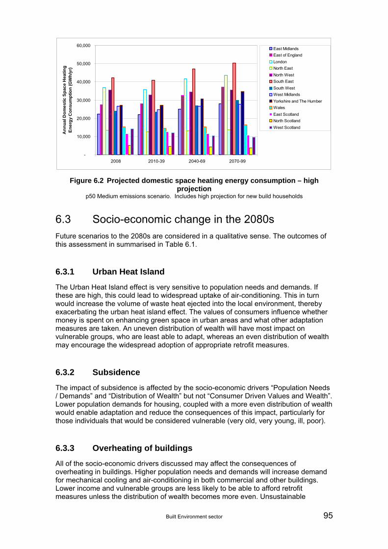
Built Environment sector 95
-
10,000
20,000
30,000
40,000
50,000
60,000
2008 2010-39 2040-69 2070-99
An
nu
al D
om
es
tic
Sp
ac
e H
ea
tin
g
En
erg
y C
on
su
mp
tio
n (
GW
h/y
r)
East Midlands
East of England
London
North East
North West
South East
South West
West Midlands
Yorkshire and The Humber
Wales
East Scotland
North Scotland
West Scotland
Figure 6.2 Projected domestic space heating energy consumption – high projection
p50 Medium emissions scenario. Includes high projection for new build households
6.3 Socio-economic change in the 2080s
Future scenarios to the 2080s are considered in a qualitative sense. The outcomes of this assessment in summarised in Table 6.1.
6.3.1 Urban Heat Island
The Urban Heat Island effect is very sensitive to population needs and demands. If these are high, this could lead to widespread uptake of air-conditioning. This in turn would increase the volume of waste heat ejected into the local environment, thereby exacerbating the urban heat island effect. The values of consumers influence whether money is spent on enhancing green space in urban areas and what other adaptation measures are taken. An uneven distribution of wealth will have most impact on vulnerable groups, who are least able to adapt, whereas an even distribution of wealth may encourage the widespread adoption of appropriate retrofit measures.
6.3.2 Subsidence
The impact of subsidence is affected by the socio-economic drivers “Population Needs / Demands” and “Distribution of Wealth” but not “Consumer Driven Values and Wealth”. Lower population demands for housing, coupled with a more even distribution of wealth would enable adaptation and reduce the consequences of this impact, particularly for those individuals that would be considered vulnerable (very old, very young, ill, poor).
6.3.3 Overheating of buildings
All of the socio-economic drivers discussed may affect the consequences of overheating in buildings. Higher population needs and demands will increase demand for mechanical cooling and air-conditioning in both commercial and other buildings. Lower income and vulnerable groups are less likely to be able to afford retrofit measures unless the distribution of wealth becomes more even. Unsustainable
96 Built Environment sector
consumer values may drive demand for air-conditioning (and associated energy), rather than using more sustainable passive cooling options. There are significant knock-on consequences for other sectors, e.g. the energy sector, depending on the adaptation measures undertaken. A large population with a high demand for air conditioning will have a high cross-sectoral impact on energy. A large population reliant on sustainable cooling measures will have less of a cross-sectoral impact.
6.3.4 Effectiveness of green space
A large population will put pressure on land, reducing the area of green space available for cooling within urban areas and could also reduce the availability of water for irrigation of green spaces during dry spells, thereby reducing their cooling effectiveness. Unsustainable consumer values could also put pressure on land and favour urban development over green space. The socio-economic driver “Distribution of Wealth” is likely to have little effect on this impact.
6.3.5 Demand for heating
Warmer winters and autonomous adaptation of people to the changing climate means that the overall impact of the socio-economic drivers is relatively low compared with the other impacts discussed. However, the distribution of wealth may have a considerable impact on affordability of heating, with vulnerable groups being most affected. High population demands, for example an increase in the numbers of households, could also increase overall heating demand, even if the per household demand decreases.
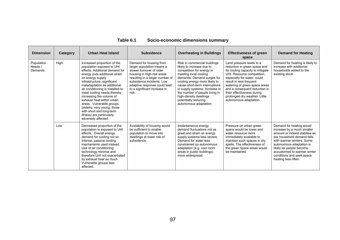
97
Table 6.1 Socio-economic dimensions summary
Dimension Category Urban Heat Island Subsidence Overheating in Buildings Effectiveness of green space
Demand for Heating
High Increased proportion of the population exposed to UHI effects. Additional demand for energy puts additional strain on energy supply infrastructure; significant maladaptation as additional air conditioning is installed to meet cooling needs thereby increasing the volume of exhaust heat within urban areas. Vulnerable groups (elderly, very young, those with short and long-term illness) are particularly adversely affected.
Demand for housing from larger population means a slower turnover of older housing in high-risk areas resulting in a larger number of subsidence incidents. Low adaptive response could lead to a significant increase in risk.
Risk in commercial buildings likely to increase due to competition for energy in meeting local cooling demands. Demand surges for cooling energy more likely to cause short-term interruptions in supply systems. Increase in the number of people living in high-density dwellings potentially reducing autonomous adaptation.
Land pressure leads to a reduction in green space and its cooling capacity to mitigate UHI. Resource competition, especially for water, could result in less frequent watering of green space areas and a consequent reduction in their effectiveness during prolonged dry weather. Little autonomous adaptation.
Demand for heating is likely to increase with additional households added to the existing stock.
Population Needs / Demands
Low Decreased proportion of the population is exposed to UHI effects. Overall energy demand for cooling not so intense, passive cooling mechanisms used instead. Use of air conditioning technology minimal and therefore UHI not exacerbated by exhaust heat as much. Vulnerable groups less affected.
Availability of housing would be sufficient to enable population to move into dwellings at lower risk of subsidence.
Instantaneous energy demand fluctuations not as great and strain on energy supply systems less severe. Demand for water less constrained so autonomous adaptation (e.g. cool room areas in public buildings) more widespread.
Pressure on urban green space would be lower and water resource more immediately available to maintain such spaces in dry spells. The effectiveness of the green space areas would be maintained.
Demand for heating would increase by a much smaller amount or indeed stabilise as per household demand falls with warmer winters. Some autonomous adaptation is likely as people become accustomed to warmer winter conditions and seek space heating less often.
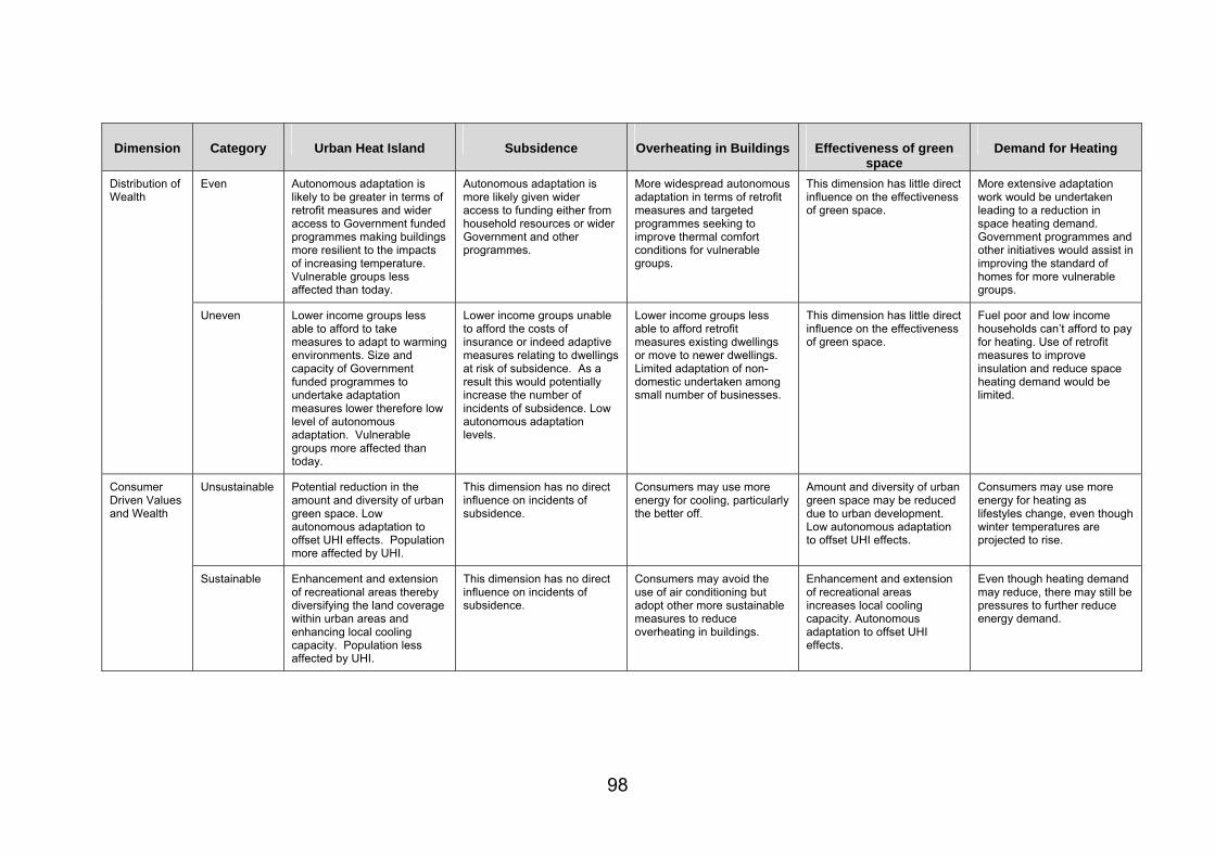
98
Dimension Category Urban Heat Island Subsidence Overheating in Buildings Effectiveness of green space
Demand for Heating
Even Autonomous adaptation is likely to be greater in terms of retrofit measures and wider access to Government funded programmes making buildings more resilient to the impacts of increasing temperature. Vulnerable groups less affected than today.
Autonomous adaptation is more likely given wider access to funding either from household resources or wider Government and other programmes.
More widespread autonomous adaptation in terms of retrofit measures and targeted programmes seeking to improve thermal comfort conditions for vulnerable groups.
This dimension has little direct influence on the effectiveness of green space.
More extensive adaptation work would be undertaken leading to a reduction in space heating demand. Government programmes and other initiatives would assist in improving the standard of homes for more vulnerable groups.
Distribution of Wealth
Uneven Lower income groups less able to afford to take measures to adapt to warming environments. Size and capacity of Government funded programmes to undertake adaptation measures lower therefore low level of autonomous adaptation. Vulnerable groups more affected than today.
Lower income groups unable to afford the costs of insurance or indeed adaptive measures relating to dwellings at risk of subsidence. As a result this would potentially increase the number of incidents of subsidence. Low autonomous adaptation levels.
Lower income groups less able to afford retrofit measures existing dwellings or move to newer dwellings. Limited adaptation of non-domestic undertaken among small number of businesses.
This dimension has little direct influence on the effectiveness of green space.
Fuel poor and low income households can’t afford to pay for heating. Use of retrofit measures to improve insulation and reduce space heating demand would be limited.
Unsustainable Potential reduction in the amount and diversity of urban green space. Low autonomous adaptation to offset UHI effects. Population more affected by UHI.
This dimension has no direct influence on incidents of subsidence.
Consumers may use more energy for cooling, particularly the better off.
Amount and diversity of urban green space may be reduced due to urban development. Low autonomous adaptation to offset UHI effects.
Consumers may use more energy for heating as lifestyles change, even though winter temperatures are projected to rise.
Consumer Driven Values and Wealth
Sustainable Enhancement and extension of recreational areas thereby diversifying the land coverage within urban areas and enhancing local cooling capacity. Population less affected by UHI.
This dimension has no direct influence on incidents of subsidence.
Consumers may avoid the use of air conditioning but adopt other more sustainable measures to reduce overheating in buildings.
Enhancement and extension of recreational areas increases local cooling capacity. Autonomous adaptation to offset UHI effects.
Even though heating demand may reduce, there may still be pressures to further reduce energy demand.

Built Environment sector 99
6.4 Relevant impacts from other sectors
This section covers the impacts that were analysed in detail within the other sectors of the CCRA, but have been included in this report as they are relevant to the built environment. The presentation format is that used in each of the sector reports, which in some cases differs from the presentation used for the Built Environment sector. In particular, some of the metrics were quantified using projections of population and property numbers.
6.4.1 Water Sector
WA5 – Water supply-demand deficit
Supply-demand balance results were calculated for each of the scenarios presented in Table 6.2. The two parameters used to define the scenarios were the change in population and per capita consumption (pcc). The population scenarios (‘High’, ‘Principal’ and ‘Low’) follow the naming convention of the population forecasts developed by ONS.
The per capita consumption values vary with anticipated adaptation. For example the current estimate of 150 l/h/d for England and Wales (Defra, 2008; Ofwat, 2010) is used for the Baseline, Climate change only and High population scenarios, while the per capita consumption values for the Principal projection scenario are based on the ambition for water consumption in the Future Water strategy, which is to reduce water consumption in England by 13 percent to 130 l/h/d (this is now being reviewed).. It should be noted that the main reason for including reductions of up to 130 l/h/d was to show the sensitivity of the supply-demand deficit to changes in water demand. While these figures give an indication of what the supply-demand deficit might be like if the demand for water was reduced, the current estimate of 150 l/h/d is more realistic (if compulsory metering is not going to be introduced).
Table 6.2 Per capita consumption (pcc) and change in population, for the climate change and socio-economic scenarios
Epoch Variable
Baseline scenario (Note 1)
Climate change
only
High population
Principal projection
(Anticipated Adaptation)
Low population
pcc (litres per person per day 150 150 150 137.4 126.4
2020s change in population
As principal
projection 0% Note 2 Note 2 Note 2
pcc (litres per person per day 150 150 150 130 101
2050s change in population
As principal
projection 0% Note 2 Note 2 Note 2
pcc (litres per person per day 150 150 150 130 83.7
2080s change in population
As principal
projection 0% Note 2 Note 2 Note 2
Note 1: Baseline scenario includes climate change and population growth (principal projection) Note 2: Data on population by river basin is given in the Water sector report

100 Built Environment sector
The only difference between the High population and the climate change only scenarios is the population growth rate; the climate change only scenario assumes no change in population whereas the High population scenario is using higher rates than the Principal projection scenario based on figures from ONS.
The Principal projection scenario has lower per capita consumption values but the same population growth rates as the Baseline scenario. The Low population scenario has lower per capita consumption and population growth rates than the Principal projection scenario. It should be noted that figures for per capita consumption were based on a former Defra ambition for England of reducing demand to 130 l/h/d, and this needs to be considered when interpreting the results.
The projected impacts of climate and socio-economic change on the water supply-demand deficit are summarised by UKCP09 river basin region in Figure 6.3. The Climate Change and Population maps show outputs for the baseline scenario while the Anticipated Adaptation maps show outputs for the Principal projection scenario (both as specified in Table 6.2).
While climate change is projected to have a large influence on the supply-demand deficit (Rance et al., 2012), Figure 6.3 shows it is also likely to be heavily influenced by population growth. This is because population changes are the main driver in determining the demand for water, which is used in the calculation of the supply-demand balance. The deficit is higher in the Climate Change and Population maps, than in the Climate Change only maps. At the UKCP09 river basin region level, the supply-demand deficit could also be affected by population movements within the country. Probably to a lesser extent, the figure shows that technological changes such as improved water efficiency measures could also affect the results for this metric.
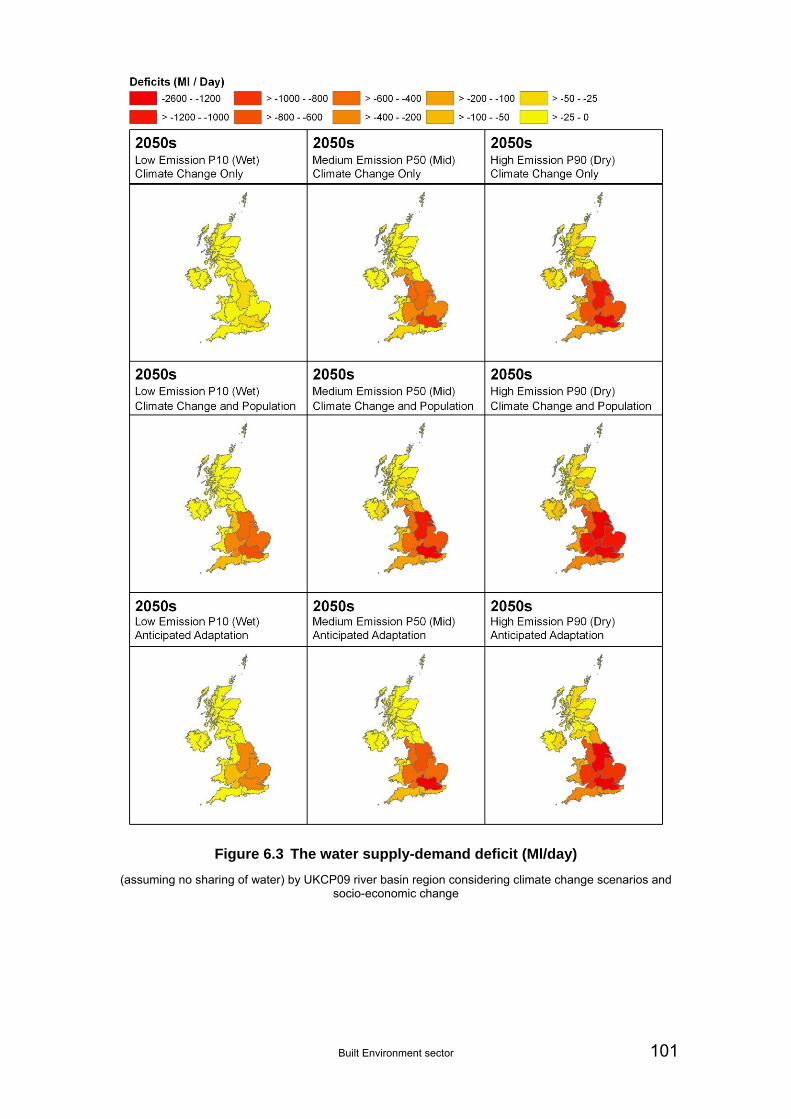
Built Environment sector 101
Figure 6.3 The water supply-demand deficit (Ml/day)
(assuming no sharing of water) by UKCP09 river basin region considering climate change scenarios and socio-economic change
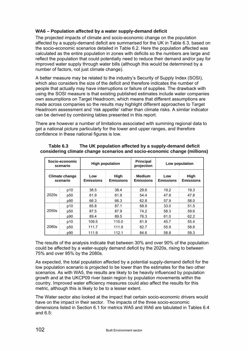
102 Built Environment sector
WA6 – Population affected by a water supply-demand deficit
The projected impacts of climate and socio-economic change on the population affected by a supply-demand deficit are summarised for the UK in Table 6.3, based on the socio-economic scenarios detailed in Table 6.2. Here the population affected was calculated as the entire population in zones with deficits so the numbers are large and reflect the population that could potentially need to reduce their demand and/or pay for improved water supply through water bills (although this would be determined by a number of factors, not just climate change).
A better measure may be related to the industry’s Security of Supply Index (SOSI), which also considers the size of the deficit and therefore indicates the number of people that actually may have interruptions or failure of supplies. The drawback with using the SOSI measure is that existing published estimates include water companies own assumptions on Target Headroom, which means that different assumptions are made across companies so the results may highlight different approaches to Target Headroom assessment and ‘risk appetite’ rather than climate risks. A similar indicator can be derived by combining tables presented in this report.
There are however a number of limitations associated with summing regional data to get a national picture particularly for the lower and upper ranges, and therefore confidence in these national figures is low.
Table 6.3 The UK population affected by a supply-demand deficit considering climate change scenarios and socio-economic change (millions)
Socio-economic scenario
High population Principal
projection Low population
Climate change scenario
Low Emissions
High Emissions
Medium Emissions
Low Emissions
High Emissions
p10 38.5 38.4 29.6 19.2 19.3 p50 61.9 61.9 54.4 47.8 47.8 2020s
p90 66.3 66.3 62.8 57.9 58.0 p10 85.8 87.1 68.9 33.0 51.5 p50 87.5 87.9 74.2 58.3 59.6 2050s
p90 89.4 89.5 76.3 61.0 62.2 p10 109.5 110.0 81.9 45.7 55.4
p50 111.7 111.9 82.7 55.9 58.8 2080s
p90 111.9 112.1 84.6 58.8 59.3 The results of the analysis indicate that between 30% and over 90% of the population could be affected by a water-supply demand deficit by the 2020s, rising to between 75% and over 95% by the 2080s.
As expected, the total population affected by a potential supply-demand deficit for the low population scenario is projected to be lower than the estimates for the two other scenarios. As with WA5, the results are likely to be heavily influenced by population growth and at the UKCP09 river basin region by population movements within the country. Improved water efficiency measures could also affect the results for this metric, although this is likely to be to a lesser extent.
The Water sector also looked at the impact that certain socio-economic drivers would have on the impact in their sector. The impacts of the three socio-economic dimensions listed in Section 6.1 for metrics WA5 and WA6 are tabulated in Tables 6.4 and 6.5:

Built Environment sector 103
Table 6.4 Socio-economic futures overview
Population needs/demands
Distribution of wealth
Consumer driven values and wealth
WA5 - Supply-demand deficits WA6 - Population affected by a supply-demand deficit
Not relevant Relevant Relevant and a stronger driver of change than climate
Table 6.5 Socio-economic futures detail
Population needs/demands (high/low)
Population numbers are the primary driver for increased water demands that affect the supply-demand balance (WA5). Under the highest population forecasts large deficits are estimated to emerge decades earlier than for the principal or central forecast. As water resources plans consider the medium term and are currently updated every five years, high populations and demands would lead to earlier investment in supply-side schemes, greater management of demands and potentially have knock-on effects for the location of new developments away from areas at greatest water stress. The mix of adaptation measures promoted may be very different under different futures, e.g. a more sustainable future may favour demand management measures and a greater emphasis on local decision making may reduce the amount of water exported to meet demand in other regions.
Distribution of wealth (even/uneven)
The distribution of wealth will have specific effects on “water poverty” and more generally the ability of lower income groups to pay utility bills.
Consumer driven values and wealth (sustainable/ unsustainable)
Consumer driven values have a major influence on the per capita consumption and household demand for water.
6.4.2 Floods and Coastal Erosion Sector
Properties at significant likelihood of flooding (Metrics FL6 and FL7)
The metrics for property show the same trends as population at significant likelihood of flooding, with a projected 45% increase in total numbers of properties at significant likelihood of flooding by the 2080s (under the ‘Principal’ population growth assumption) compared with the climate change only case.
The overall numbers are summarised in Tables 6.6 (properties) and 6.7 (EAD) for the p50 Medium emissions scenario and the ‘principal’ population growth assumption. Ranges for combinations of climate and socio-economic scenarios are also shown.
Table 6.6 Properties at significant likelihood of flooding
Climate change only With population growth Low projection High projection2020s 990 1,120 760 1,370
2050s 1,220 1,580 840 2,100
2080s 1,340 1,950 1,040 2,850
Properties at risk (thousands)Range of projections (combining climate and socioeconomic scenarios)
Epoch Properties at risk (thousands)P50 Medium Emissions climate change scenarioPrincipal population projection

104 Built Environment sector
Table 6.7 EAD for properties at likelihood of flooding
Climate change only With population growth Low projection High projection2020s 2,210 2,380 1,520 3,500
2050s 2,960 3,840 1,770 6,760
2080s 3,750 5,440 2,190 11,590
Epoch Expected Annual damages (£ millions) Expected Annual damages (£ millions)P50 Medium Emissions climate change scenario Range of projections (combining climate and socioPrincipal population projection economic scenarios)
The ‘Low’ projections are based on the p10 Low or Medium emissions scenario and low population growth. The ‘High’ projections are based on the p90 Medium or High emissions scenario and high population growth.
The projected number of properties at significant likelihood of flooding in the 2080s for the five climate change scenarios is from 1.0 to 2.9 million. The projected range of EAD for properties in the 2080s for the five climate change scenarios is from about £2 billion to £12 billion.
Residential properties at significant likelihood of flooding (to assess insurance impacts) (Metric FL13)
Projections for the number of residential properties exposed to a 1.3% (1:75) flood probability or greater (i.e. at significant likelihood of flooding) is covered by Metric 6a. The total numbers are given in Table 6.8 below.
Table 6.8 Residential properties at significant likelihood of flooding: median estimate
Climate change only With population growth
Low projection High projection
2020s 690 780 510 9702050s 870 1130 580 15102080s 960 1400 730 2080
Epoch Residential properties at risk (thousands)P50 Medium Emissions climate change scenarioPrincipal population projection
Residential properties at risk (thousands)Range of projections (combining climate and socio economic scenarios)
The ‘Low’ and ‘High’ projections are the same as those used in Tables 6.6 and 6.7. The projected range is between about 730,000 and 2.1 million properties by the 2080s.
Socio-economic dimensions
The effects that socio-economic dimensions would have on the impact of changes in flood and coastal erosion risk were considered in the Floods and Coastal Erosion sector report including the following dimensions considered in this section:
Population needs/demands (high/low)
Distribution of wealth (even/uneven)
Consumer driven values and wealth (sustainable/unsustainable).
Population needs/demands (high/low) affects the increase in number of people exposed to flood risk. One extreme is that there is a high degree of demand for development, where more people are exposed to flood risks. The other is that demand is low, and the number of additional people exposed to risk is small.
With regard to the distribution of wealth (even/uneven), where the distribution of wealth is more even, overall flood risk is likely to reduce. This is because more people would

Built Environment sector 105
be able to implement risk management measures including suitable insurance and possibly flood proofing of properties.
Where the distribution of wealth is more uneven, the number of people who are less able to implement risk management measures is likely to increase. There is already evidence to show that, proportionally, there are more poorer communities in flood risk areas than richer communities (Environment Agency, 2006), and this trend would continue.
As the poorer communities would be less able to take such measures as adequate flood insurance and contingency planning, flooding would have a more severe impact leading to a widening of the gap between rich and poor (and increasing demands on Government to support the poor).
The two extremes of consumer driven values and wealth could be considered as ‘unsustainable’ and ‘sustainable’ respectively. The unsustainable approach could lead to greater investment in flood risk management assets to protect the increasing wealth, but at the same time would lead to an overall increase in vulnerability as the number of assets in the floodplains increase.
In the long term this approach could leave a legacy of high flood risk and high asset maintenance requirements, which could prove a burden for future generations.
The sustainable approach would concentrate on flood risk management solutions that reduce the burden on future generations, by minimising increases in flood risk and reducing risk wherever possible (as encapsulated in Defra’s ‘Making Space for Water’ policy).
6.4.3 Health Sector
HE1 – Temperature mortality (Heat) and HE5 Temperature mortality (Cold)
Heat and cold affected deaths are a function of several factors, including the age distribution of the population of a region, levels of deprivation (especially in relation to cold related deaths), and social capital (i.e. social networks and contacts). This could have an effect on the baseline mortality rates, as well as the heat and cold mortality slopes and thresholds.
However, the relationship between temperature related mortality, deprivation and social capital is very complex and not possible to characterise within this assessment. It is also believed that there is limited published research in this area (Wolf et al., 2010; Hajat et al., 2007; Wilkinson et al., 2004). For the purpose of this assessment, baseline mortality rates, as well as temperature related mortality slopes and thresholds are assumed to remain unchanged in the future, and heat and cold related mortality are therefore considered to be solely proportional to population sizes.
Results for deaths brought forward (heat) and premature deaths avoided (cold) are therefore given for low, principal and high population projections for the 2020s, 2050s and 2080s based on the population projections. Summary statistics for the UK as a whole are given in Tables 6.9 to 6.14. Ranges are given for deaths avoided (cold) owing to uncertainty over the relevant temperature thresholds that could cause death.

106 Built Environment sector
Table 6.9 Additional deaths brought forward (heat) per year for the UK for the different emissions scenarios
(low population projection, baseline period: 1993-2006)
2020s 2050s 2080s Scenario
p10 p50 p90 p10 p50 p90 p10 p50 p90
Low 633 1899 4196 1086 2956 6503Medium 139 768 1795 929 2440 5278 1816 4606 9952High 1217 3051 6473 2985 7198 15031
Table 6.10 Additional deaths brought forward (heat) per year for the UK for the different emissions scenarios
(principal population projection, baseline period: 1993-2006)
2020s 2050s 2080s Scenario
p10 p50 p90 p10 p50 p90 p10 p50 p90
Low 700 2095 4627 1451 3946 8667Medium 145 804 1878 1095 2878 6224 2500 6336 13682High 1345 3370 7144 3985 9600 20017
Table 6.11 Additional deaths brought forward (heat) per year for the UK for the different emissions scenarios
(high population projection, baseline period: 1993-2006)
2020s 2050s 2080s Scenario
p10 p50 p90 p10 p50 p90 p10 p50 p90
Low 866 2602 5744 1959 5332 11711Medium 152 841 1965 1272 3343 7227 3279 8306 17930High 1668 4180 8862 5388 12986 27076
Table 6.12 Premature deaths avoided (Cold) per year for the UK for the different emissions scenarios
(low population projection, baseline period: 1993-2006)
2020s 2050s 2080s Scenario
p10 p50 p90 p10 p50 p90 p10 p50 p90
4181 8628 13305 5917 10805 15855 Low 6342 13270 20823 9033 16786 25222
1348 4792 8364 5423 9983 14867 8180 13502 18928 Medium
2028 7282 12850 8254 15421 23426 12581 21223 30700
6480 11275 16319 10833 16532 21946 High
9897 17501 25897 16830 26403 36536
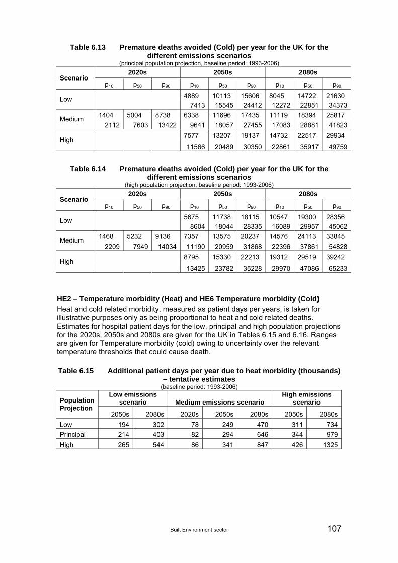
Built Environment sector 107
Table 6.13 Premature deaths avoided (Cold) per year for the UK for the different emissions scenarios
(principal population projection, baseline period: 1993-2006)
2020s 2050s 2080s Scenario
p10 p50 p90 p10 p50 p90 p10 p50 p90
4889 10113 15606 8045 14722 21630 Low 7413 15545 24412 12272 22851 34373
1404 5004 8738 6338 11696 17435 11119 18394 25817 Medium
2112 7603 13422 9641 18057 27455 17083 28881 41823
7577 13207 19137 14732 22517 29934 High
11566 20489 30350 22861 35917 49759
Table 6.14 Premature deaths avoided (Cold) per year for the UK for the different emissions scenarios
(high population projection, baseline period: 1993-2006)
2020s 2050s 2080s Scenario
p10 p50 p90 p10 p50 p90 p10 p50 p90
5675 11738 18115 10547 19300 28356 Low 8604 18044 28335 16089 29957 45062
1468 5232 9136 7357 13575 20237 14576 24113 33845 Medium
2209 7949 14034 11190 20959 31868 22396 37861 54828
8795 15330 22213 19312 29519 39242 High
13425 23782 35228 29970 47086 65233
HE2 – Temperature morbidity (Heat) and HE6 Temperature morbidity (Cold)
Heat and cold related morbidity, measured as patient days per years, is taken for illustrative purposes only as being proportional to heat and cold related deaths. Estimates for hospital patient days for the low, principal and high population projections for the 2020s, 2050s and 2080s are given for the UK in Tables 6.15 and 6.16. Ranges are given for Temperature morbidity (cold) owing to uncertainty over the relevant temperature thresholds that could cause death.
Table 6.15 Additional patient days per year due to heat morbidity (thousands) – tentative estimates
(baseline period: 1993-2006) Low emissions
scenario Medium emissions scenario High emissions
scenario Population Projection
2050s 2080s 2020s 2050s 2080s 2050s 2080s
Low 194 302 78 249 470 311 734
Principal 214 403 82 294 646 344 979
High 265 544 86 341 847 426 1325
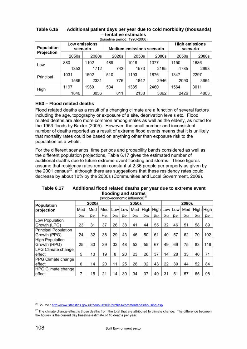
108 Built Environment sector
Table 6.16 Additional patient days per year due to cold morbidity (thousands) – tentative estimates
(baseline period: 1993-2006) Low emissions
scenario Medium emissions scenario High emissions
scenario Population Projection
2050s 2080s 2020s 2050s 2080s 2050s 2080s
880 1102 489 1018 1377 1150 1686 Low 1353 1712 743 1573 2165 1785 2693
1031 1502 510 1193 1876 1347 2297 Principal 1586 2331 776 1842 2946 2090 3664
1197 1969 534 1385 2460 1564 3011 High 1840 3056 811 2138 3862 2426 4803
HE3 – Flood related deaths
Flood related deaths as a result of a changing climate are a function of several factors including the age, topography or exposure of a site, deprivation levels etc. Flood related deaths are also more common among males as well as the elderly, as noted for the 1953 floods by Baxter (2005). However, the small number and inconsistent number of deaths reported as a result of extreme flood events means that it is unlikely that mortality rates could be based on anything other than exposure risk to the population as a whole.
For the different scenarios, time periods and probability bands considered as well as the different population projections, Table 6.17 gives the estimated number of additional deaths due to future extreme event flooding and storms. These figures assume that residency rates remain constant at 2.36 people per property as given by the 2001 census26, although there are suggestions that these residency rates could decrease by about 10% by the 2030s (Communities and Local Government, 2009).
Table 6.17 Additional flood related deaths per year due to extreme event flooding and storms
(socio-economic influence)27
2020s 2050s 2080s
Med Med Med Low Low Med High High Low Low Med High HighPopulation projection
p10 p50 P90 p10 p50 p50 p50 p90 p10 p50 p50 p50 p90 Low Population Growth (LPG) 23 31 37 26 38 41 44 55 32 46 51 58 89 Principal Population Growth (PPG) 24 32 38 29 43 46 50 61 40 57 62 70 102High Population Growth (HPG) 25 33 39 32 48 52 55 67 49 69 75 83 116LPG Climate changeeffect 5 13 19 8 20 23 26 37 14 28 33 40 71 PPG Climate changeeffect 6 14 20 11 25 28 32 43 22 39 44 52 84 HPG Climate changeeffect 7 15 21 14 30 34 37 49 31 51 57 65 98
26 Source : http://www.statistics.gov.uk/census2001/profiles/commentaries/housing.asp.
27 The climate change effect is those deaths from the total that are attributed to climate change. The difference between the figures is the current day baseline estimate of 18 deaths per year.

Built Environment sector 109
6.4.4 Business Sector
The potential impacts of the three socio-economic drivers listed in Section 6.1 on Business sector metrics BU6 and BU10 are discussed in Table 6.18.
Table 6.18 Business sector socio-economic summary: Projections to 2080
Socio-economic Factor
BU6 Mortgage provision
BU10 Over heating
Population needs/demands (high/low)
Increasing populations may exacerbate the issue of homes and floodplains. If unmanaged, house stock asset value may be affected if insurance becomes increasingly unavailable.
Risk in commercial buildings likely to increase due to competition for energy in meeting local cooling demands. Demand surges for cooling energy more likely to cause short-term interruptions in supply systems.
Distribution of wealth (even/uneven)
The housing market is sensitive to the distribution of wealth. The loss of mortgage provision could lead to poorer people living in flood risk areas without insurance, hence increasing vulnerability.
More widespread autonomous adaptation in terms of retrofit measures and targeted programmes seeking to improve thermal comfort conditions but SMEs may lag behind larger businesses.
Consumer driven values and wealth (sustainable/ unsustainable)
Increasing demand for homes and wealth may exacerbate issues around flood risk and mortgage provision.
Not applicable
6.4.5 Energy Sector
EN2 – Energy demand for cooling
Analysis by Day et al. (2009) and DECC (2010c) take into consideration increases in building stock and therefore take socio-economic change into account. Currently there is one area that does not contribute significantly to cooling demand: the domestic or residential sector. This is likely to change in the future due to an increase in population as well as an increase in market penetration of air-conditioning. Day et al. (2009) analysed an accelerated demand in the residential sector in London; this resulted in 10% of residential properties with mechanical cooling by 2030 (approximately 300,000 residencies) accounting for 0.28TWh of energy. In the future there may be increased expectations that new builds include cooling systems. Day et al. (2009) state that a key issue for the residential sector is to ensure that high efficiency cooling systems are designed into new development otherwise poorer systems may by installed at a later date.
There are many potential socio-economic scenarios that are likely to affect cooling demand including population growth, mitigation policy and behavioural change. In future CCRA updates these should be considered in more detail.

110 Built Environment sector
7 Costs of Climate Change Climate change adaptation decisions that are designed to reduce climate change risks inevitably involved making trade-offs concerning the use of scarce economic resources. To the extent that economic efficiency is an important criterion in informing such decision-making, it is useful to express climate change risks in monetary terms, so that they can be:
Assessed and compared directly (using £ as a common metric) and
Compared against the costs of reducing such risks by adaptation.
For the CCRA, a monetisation exercise has been undertaken to allow an initial comparison of the relative importance of different risks within and between sectors. Since money is a metric with which people are familiar, it may also serve as an effective way of communicating the possible extent of climate change risks in the UK and help raise awareness.
Where possible, an attempt has been made to express the size of individual risks (as described in this report) in monetary terms (cost per year) however, due to a lack of available data it has sometimes been necessary to use alternative costs (repair or adaption) to provide an estimate.
A variety of methods have been used to determine the costs. In broad terms, these methods can be categorised according to whether they are based on:
Market prices (MP)
Non-market values (NMV) or
Informed judgement (IJ).
Informed judgement has been used where there is no quantitative evidence and was based on extrapolation and/or interpretation of existing data.
In general terms, these three categories of method have differing degrees of uncertainty attached to them, with market prices being the most certain and informed judgement being the least certain. It is important to stress that the confidence and uncertainty of consequences differs. Therefore, care must be taken in directly comparing the results. Whilst we attempt to use the best monetary valuation data available, the matching-up of physical and monetary data is to be understood as an approximation only.
Further, it is important to highlight that some results are presented for a scenario of future climate change only, whilst others include climate change under assumptions of future socio-economic change. There are also some important cross-sector links, or areas where there is the risk of double counting impacts: these are highlighted on table 7.1.
A large proportion of this chapter is devoted to metric BE9 (demand for heating). This is because (a) it has a large economic impact and (b) the analysis also includes the economic benefits of reductions in GHG and air pollution emissions.
7.1 Summary of the results
A summary of the results is provided in Table 7.1. It is stressed that the pedigree, confidence and uncertainty of different impact categories differ, thus care must be

Built Environment sector 111
taken in directly comparing the results. Further, it is important to highlight that some results are presented for a scenario of future climate change only, whilst others include climate change under assumptions of future socio-economic change28. The approach used is stated in Table 7.1. There are also some important cross-sectoral links, or areas where there is the risk of double counting impacts: these are highlighted on the table.
Table 7.1 shows that one risk, reduction in heating demand (metric BE9), has monetary impacts ranked as ‘very high’ (£billion/year), although the impact is positive rather than negative: this positive effects also needs to be compared against the negative impacts of overheating of buildings (metric BE3), and the additional cooling costs (energy sector metric EN2). A number of other metrics have ‘high’ negative risks (>£100 million/year), including overheating of buildings. Other metrics have a medium or low ranking attached to them.
The study has applied quantitative estimates to all metrics that were quantified in the Tier 2 analysis (i.e. BE2 and BE9). Where quantitative risk data does not exist, it has been necessary to use expert judgement within the CCRA team to provide indicative estimates. These estimates (BE1, BE3, BE4, and BE5) should be treated with less confidence, i.e. they are only indicative. A number of other metrics were considered in the earlier analysis but are not reported on in this sector report. Note that the reason for their omission is because they are covered in other sectors (water availability/demand and floods), or else they were highlighted as potential areas for future investigation.
This section also presents the results of the monetisation analysis for the risk metrics from other sectors that have been covered in the previous analysis sections of this report, owing to their close links with the Built Environment sector.
28 The combined effects of socio-economic and climate change together provides the total risks faced, but care should be taken when attributing the relative (or marginal) risk due to climate change specifically, as this only includes the climate related element.
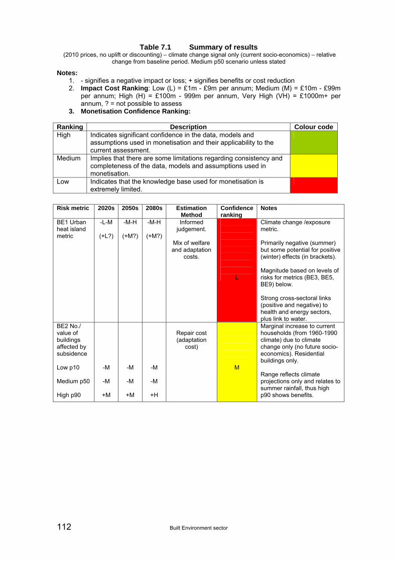
112 Built Environment sector
Table 7.1 Summary of results (2010 prices, no uplift or discounting) – climate change signal only (current socio-economics) – relative
change from baseline period. Medium p50 scenario unless stated
Notes: 1. - signifies a negative impact or loss; + signifies benefits or cost reduction 2. Impact Cost Ranking: Low (L) = £1m - £9m per annum; Medium (M) = £10m - £99m
per annum; High (H) = £100m - 999m per annum, Very High (VH) = £1000m+ per annum, ? = not possible to assess
3. Monetisation Confidence Ranking: Ranking Description Colour code High Indicates significant confidence in the data, models and
assumptions used in monetisation and their applicability to the current assessment.
Medium Implies that there are some limitations regarding consistency and completeness of the data, models and assumptions used in monetisation.
Low Indicates that the knowledge base used for monetisation is extremely limited.
Risk metric 2020s 2050s 2080s Estimation Method
Confidence ranking
Notes
BE1 Urban heat island metric
-L-M
(+L?)
-M-H
(+M?)
-M-H
(+M?)
Informed judgement.
Mix of welfare and adaptation
costs.
L
Climate change /exposure metric. Primarily negative (summer) but some potential for positive (winter) effects (in brackets). Magnitude based on levels of risks for metrics (BE3, BE5, BE9) below. Strong cross-sectoral links (positive and negative) to health and energy sectors, plus link to water.
BE2 No./ value of buildings affected by subsidence Low p10 Medium p50 High p90
-M
-M
+M
-M
-M
+M
-M
-M
+H
Repair cost (adaptation
cost)
M
Marginal increase to current households (from 1960-1990 climate) due to climate change only (no future socio-economics). Residential buildings only. Range reflects climate projections only and relates to summer rainfall, thus high p90 shows benefits.

Built Environment sector 113
Table 7.1 Summary of results (continued) Costs in £million per annum (2010 prices, no uplift or discounting) – climate change only (current socio-
economics) – relative change from baseline period. Risk metric 2020s 2050s 2080s Estimation
Method Confidence ranking
Notes
BE3 Overheating of non-domestic buildings * Low p10 Medium p50 High p90
-L
-M
-M
-L
-M
-M
-L
-H
-H-VH
Informed judgement
L
Climate only (no change in offices or productivity over time). Assumes no autonomous adaptation or use of cooling (energy), thus values are considered high. Note overlap with BU10, which addresses similar impact. Also, strong overlap (double counting) with increased energy use (EN3) in energy sector analysis. Range shows climate projection only.
* Note: that there is also the effect of overheating on residential buildings (health impacts, discomfort and disamenity, sleep disturbance, and energy costs). Health impacts and potential energy costs (cooling) are captured in the health and energy sector report: note that the combined economic effects of overheating to
residential buildings are possibly larger than non-domestic buildings. BE4 Cultural heritage at flood risk.
See Floods and Coastal Erosion sector report Probably modest costs (M) but potentially some nationally important issues of concern.
BE5 Effectiveness of green space in reducing urban temperature. Low p10 Medium p50 High p90
0
-L
-L
0
-L
-M
-L
-M
-M-H
Informed judgement
L
Climate change /exposure metric. Linkages to (BE3, BE9) as well as feedbacks with BE1. Strong cross-sectoral links to health and energy sectors, and some links to water. Range reflects climate only (increasing aridity). Excludes additional recreational value (NMV) for use of space itself.

114 Built Environment sector
Table 7.1 Summary of results (continued) Costs in £million per annum (2010 prices, no uplift or discounting) – climate change only (current socio-
economics) – relative change from baseline period. Risk metric 2020s 2050s 2080s Estimation
Method Confidence ranking
Notes
BE9 Indicative number of heating days (residential) # / ## Low p10 Medium p50 High p90
+H
+H
+VH
+VH
+VH
+VH
+VH
+VH
+VH
Market prices
Energy costs – long-run
variable costs for residential sector based
on DECC guidance.
H
Climate change only (current socio-economics), for current stock. Not include existing policy, notably green deal, thus probable over-estimate. Note no rebound effects included, which would reduce benefits significantly. Range reflects climate only.
Ancillary effects Low p10 Medium p50 High p90
+H
+H
+H
Non market values
Reduced GHG and air
pollution
H
Additional ancillary benefits of reductions, assuming gas provides future demand - note later time periods assume low carbon energy.
# Note there is also a reduction in heating demand for non-residential buildings. Current energy used in non-residential space heating is around 40% of residential demand, thus including these benefits would
further increase the benefits in BE9 above. ## Note there are also increases in cooling demand for residential buildings, and increased energy cooling
costs as well as health impacts, discomfort and disamenity, sleep disturbance. Health impacts and potential energy costs (cooling) are captured in the Health and Energy sector reports.
WA5 – Supply-demand deficits Low p10 Medium p50 High p90
+H
+M
-H
+M
-H
-H
-M
-H
-H
Market Prices H
Supply costs used. These equate to adaptation costs and are used to proxy welfare costs, only. Note consideration of climate and socio-economics increases deficit and total costs, though still in same bands.
WA6 - Population affected by supply-demand deficit
-M -M -M Informed
Judgement L
Metric largely covered by WA5. Cost ranking based only on possible impacts on households not connected to mains, and businesses with high WTP not captured in WA5.
FL6 No. residential properties and EAD
-H -H -VH Market Prices H
Property damage costs based on replacement costs and can be seen as adaptation costs.
FL7 EAD commercial properties; counts of commercial property types
-H -H -VH Market Prices H
Property damage costs based on replacement costs and can be seen as adaptation costs.
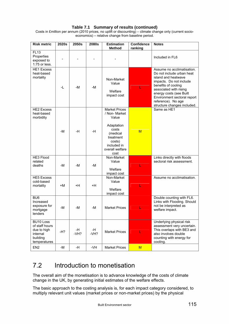
Built Environment sector 115
Table 7.1 Summary of results (continued) Costs in £million per annum (2010 prices, no uplift or discounting) – climate change only (current socio-
economics) – relative change from baseline period. Risk metric 2020s 2050s 2080s Estimation
Method Confidence ranking
Notes
FL13 Properties exposed to 1:75 or less.
- - - - Included in FL6
HE1 Excess heat-based mortality
-L -M -M
Non-Market Value
Welfare
impact cost
L
Assume no acclimatisation. Do not include urban heat island and heatwave impacts. Do not include benefits of cooling associated with rising energy costs (see Built Environment sectoral report reference). No age structure changes included.
HE2 Excess heat-based morbidity
-M -H -H
Market Prices / Non- Market
Value
Adaptation costs
(medical treatment
costs) included in
overall welfare cost
M
Same as HE1
HE3 Flood related deaths -M -M -M
Non-Market Value
Welfare
impact cost
L
Links directly with floods sectoral risk assessment.
HE5 Excess cold-based mortality +M +H +H
Non-Market Value
Welfare
impact cost
L
Assume no acclimatisation.
BU6 Increased exposure for mortgage lenders
-M -M -M Market Prices L
Double counting with FL6. Links with Flooding. Should not be interpreted as welfare impact.
BU10 Loss of staff hours due to high internal building temperatures
-H? -H
-VH? -H
-VH? Market Prices L
Underlying physical risk assessment very uncertain. This overlaps with BE3 and also involves double counting with energy for cooling.
EN2 -M -H -VH Market Prices M
7.2 Introduction to monetisation
The overall aim of the monetisation is to advance knowledge of the costs of climate change in the UK, by generating initial estimates of the welfare effects.
The basic approach to the costing analysis is, for each impact category considered, to multiply relevant unit values (market prices or non-market prices) by the physical
116 Built Environment sector
impacts identified in earlier sections of this sector report. The total value to society of any risk is taken to be the sum of the values of the different individuals affected. This distinguishes this system of values from one based on ‘expert’ preferences, or on the preferences of political leaders. However, due to the availability of data, it has sometimes been necessary to use alternative approaches (e.g. repair or adaptation costs) to provide indicative estimates.
There are a number of methodological issues that have to be addressed in making this conversion (Metroeconomica, 2006) including the compatibility between physical units and monetary units and the selection of unit values that address market and non-market impacts. As far as possible, physical and monetary units have been reconciled. The selection of unit values is justified in the explanation of the method used to monetise each risk metric. The aim is to express the risk in terms of its effects on social welfare, as measured by the preferences of individuals in the affected population. Individual preferences are expressed in two, theoretically equivalent, ways. These are:
The minimum payment an individual is willing to accept (WTA) for bearing the risk or
The maximum amount an individual is willing to pay (WTP) to avoid the risk.
There are also other issues (beyond this scoping analysis) in terms of impacts that have non-marginal effects on the UK economy, the treatment of distributional variations in impacts, and the aggregation of impact cost estimates over sectors and time.
7.3 Presentation of results
The analysis by metric is presented in Sections 7.4 to 7.18.
The climate scenarios are those adopted across the CCRA i.e. the UKCP09 scenarios: Low, Medium and High. No specific mitigation assumptions have been used in the analysis, though a discussion of these aspects is included in Section 9. For each climate scenario, a probabilistic density function (pdf) has been generated; the CCRA has used data from the 10% (p10, p50), 50% (p50) and 90% (p50, p90) of this pdf. Four population scenarios are adopted for various metrics: Current, Low, Principal and High.
Consistent with other sectors, the results below are presented in terms of constant 2010 prices) for the three time periods considered in the CCRA i.e. the 2020s, 2050s and 2080s. The results are presented in this way to facilitate direct comparison.
At this stage, the values are not presented as a present value or equivalent annual cost. However, the use of the values in subsequent analysis, for example in looking at the costs and benefits of adaptation options to reduce these impacts, would need to work with present values. For this, the values below would need to be adjusted and discounted. For discounting, the Green Book recommends 3.5% discount rates/factors (HMT, 2007).
Built Environment sector 117
7.4 BE1 Urban Heat Island
7.4.1 Outputs from the risk assessment
The BE1 risk metric considers the uplift in urban temperature (the urban heat island effect) in comparison to neighbouring rural locations. As urban heat island effects are not included in UKCP09, the analysis of this metric in the CCRA has been qualitative (see Section 5.4), and provides an indicative metric of the change in mean average minimum summer temperature.
Section 5.4 identifies that UHI effects will lead to a potential increase in health risks (temperature related mortality and morbidity) from the increased urban heat island effect, including increased night-time temperatures. It also identifies the additional triggering of the current heat alert (assuming current thresholds are maintained). Additional effects would also arise from increased residential and commercial building overheating, and thus discomfort, productivity losses or increased cooling demand. The CCRA has considered all of these impacts in other built environment, health or energy metrics (though these have not considered the additional impact of the urban heat island effect). Note that while the focus in Section 5.4 has been on the impacts of this metric, it is possible the UHI effect might also lead to positive benefits.29
7.4.2 Methodology and unit values to be adopted
BE1 is a climate metric, rather than an exposure or impact metric. It is therefore difficult to assess the potential economic costs of this risk, even in approximate terms. The analysis has considered the potential economic costs from considering the possible increase in other relevant metrics for health (HE1, HE2), building overheating (BE3, BU10) and energy use (EN3), which lead to some of the large economic costs (millions or even billions/year in later time periods). This provides only a very indicative estimate.
7.4.3 Results and discussion
Section 5.4 set out the relative increases indicated for this metric. Based on the size of the potential increases in UHI, and the economic costs associated with climate related increases for health (HE1, HE2), energy (cooling) and built environment (BE3), the potential economic costs of this metric could be in the range of £10 million – £99 million a year in the 2020s and plausibly £100 million – £999 million in later time periods. While it is considered that the summer related effects would lead to large negative impacts, the possibility of some positive winter effects are not ruled out. It is stressed that these estimates are very indicative only, but they do highlight the potential importance for future research in this area.
29 The urban heat island problem is discussed in Section 5.4 in the context of summer temperature, however, urban areas also have positive heat island effects in reducing cold winter temperatures, thus it is also possible that there could be some benefits in reducing winter related mortality and winter heating demand associated with this metric.

118 Built Environment sector
7.5 BE2 Subsidence
7.5.1 Outputs from the risk assessment
The BE2 risk metric considers residential building subsidence, reflecting the increased risks from drying out of vulnerable soil areas, leading to foundation damage and an increased incidence of (domestic) building subsidence.
Subsidence already has major economic consequences. As highlighted earlier, it is the second most important hazard to property insurers in the UK. Insurance claims for the period 2002 to 2009 exceeded £1.8 billion, an average of over £200 million per year. Claims in 2003 when there was a very hot summer were about £400 million. In the most recent year for which data were obtained, 2009, there were 29,700 notified domestic subsidence claims, with a total value of £175m.
The metric has been assessed in Section 5 using a response function relating the change in average summer rainfall with the projected number of notified claims (as an indicator of incidents of subsidence). Note that Section 5 considered that given the small sample size, the results are highly uncertain.
It is highlighted that this risk has a strong distributional pattern, with most risk in certain areas of England (see Figure 4.2, hence there are no DA values) and that it exists primarily for the existing housing stock (i.e. older dwellings with less resilient foundations: new build houses are considered to be better at addressing subsidence risks through building regulations). This potentially negates the need for future socio-economic projections of future housing increases, and indeed the stock at risk could reduce slightly in future years as old stock is replaced.
7.5.2 Methodology and unit values to be adopted
Previous studies have assessed the costs of subsidence from climate change, including Dlugolecki (2004) and Hunt and Taylor (2006). The former estimated subsidence claims rising from £300 million (year 2000 price) as a current annual average to £600 million in 2050 (and double this for an extreme year). The latter study estimated impacts of £5 to 15 million in the 2020s, rising to £25 to 185 million in the 2050s and £115 to 315 million in the 2080s. Note that the latter only applied the approach to extreme years (e.g. as 2003) rather than applying a general non-threshold linear analysis for lower precipitation, and so constitute a lower bound.
In order to estimate the welfare impact on the number of physical cases of building subsidence, ideally the willingness to pay of a household to avoid the risk of subsidence would be measured. In a perfect market this would be captured by the difference between the market price of a property with subsidence risk and one without this risk. Whilst this measure is likely to more fully reflect the welfare cost of the subsidence impact, the data requirements and subsequent treatment for this type of analysis (known as hedonic analysis) are much more involved than the replacement cost measure. Consequently, no estimates have been made to date.
As a result, the expenditure incurred to replace (or restore) the asset is estimated in unit cost terms. The replacement cost-based measure can be seen as a robust lower bound estimate of the welfare costs associated with subsidence. It is also, of course, a measure of adaptation costs (a reactive based response, rather than a proactive approach).

Built Environment sector 119
A unit value of £10,000 was used by Graves & Phillipson (2000) and Driscoll & Crilly (2000) in their analyses of climate change impacts on subsidence incidence for the Building Research Establishment. These estimates are derived from the typical costs of undertaking specific remedial work in the event of property subsidence. By way of comparison, aggregate historical data on subsidence claims supplied by the ABI for Great Britain can also be used to derive unit values. Using a regression analysis, Metroeconomica (2006) derived a central unit cost per subsidence of £5,650, with a lower bound of £1,500 and an upper bound of £12,000. The uncertainty reflected in this range of unit costs, together with the under-estimation implied by excluding other welfare cost components such as the disruption endured as the repair work is undertaken, leads to a unit value of £10,000 as a central value.
It is stressed that the real unit costs of subsidence work would change over time. There are possible scenarios in which the labour intensive nature of this work increases in cost, but it is also possible that they might reduce due to advances in technology.
Note that there are also some potential impacts on non-residential buildings. The most important of these are likely to be buildings or areas of cultural or historic significance, as commercial buildings are not (generally) considered to be vulnerable to subsidence. Hunt and Taylor (2006) explored the potential valuation of cultural heritage from climate change risks, using contingent valuation with a case study on a number of such buildings, and concluded that these effects are potentially significant, not least due to the high willingness to pay for protection of cultural heritage buildings from the impacts of climate change.
7.5.3 Results and discussion
The aggregated results for England are presented in Table 7.2, showing the costs of increased claims as a result of climate change (only). A full breakdown of the total number of annual claims, as well as the marginal estimated annual cases is presented by English region in Appendix 6. The results reflect the impacts of climate change only (no socio-economic change is considered, due to the lower risks for new build). Given the underlying rock and soil structure there are a number of English regions, as well as the Devolved Administrations, where this is the case.
At the UK level, the results indicate possible changes of the order of £10 million – £100 million/year (current prices, no uplifts or discounting) for England. However, there is a very wide range of results, especially when considering the regional breakdown (see Appendix 6). Even at the national level, the full uncertainty range leads to very different results, with even positive values projected in the 2080 high p90 analysis (because of increases in for summer precipitation).
The results in Appendix 6 show that by far the most vulnerable region is London, where the projected damage costs attributable to climate change (above baseline levels) vary between £12million/annum and £62million/annum over the time periods and climate scenarios. The East and South-East England regions account for the majority of the remaining damage costs in a given time period.

120 Built Environment sector
Table 7.2 Marginal change in domestic subsidence incidents per annum (BE2)
Change due to projected climate change in the 2020s, 2050s and 2080s, compared to 1961-1990 climate (2008 households, no socio-economic change). (£m per year, 2010 prices, no uplift or discounting)
2020s
Medium Medium MediumNation p10 p50 p90
England -68 -20 +38
2050s
Low Low Medium High High Nation p10 p50 p50 p50 p90
England -98 -36 -50 -52 +24
2080s
Low Low Medium High High Nation p10 p50 p50 p50 p90
England -104 -41 -61 -78 +17
Notes: + signifies that these are benefits or cost reductions.
7.6 BE3 Overheating of non-domestic buildings
7.6.1 Outputs from the risk assessment
The BE3 risk metric estimates the overheating of non-domestic buildings and thus the risks to working conditions and productivity (due to design which has become inadequate for the conditions or lack of cooling capacity). It includes commercial buildings (e.g. offices) and public buildings (e.g. schools and hospitals).
As noted in the earlier section, heat comfort levels are linked to general productivity at work; a Centre for Economics and Business Research study (CEBR, 2003) suggests that productivity falls by 8% at 26°C, by 29% at 32°C and by 62% at 38°C. The respective costs to the UK economy of these productivity falls were estimated at the time as £35m, £126m and £270m per day. In addition to lost productivity, previous heat wave events have also been characterised by travel disruption, affecting work hours, and absenteeism, all resulting in lost work time30.
The CCRA BE3 metric uses external temperature as a proxy for indoor thermal comfort in naturally ventilated buildings, and thus a proxy for comfortable conditions. It has investigated the use of a threshold based on CIBSE guidance (CIBSE, 2006) for an overheating threshold of 28°C for any building space. The CIBSE guidance recommends this threshold should not be exceeded for more than 1% of occupied hours. 30 There is some data reported in City of London (2007). Rising to the Challenge-The City of London Corporation’s Climate Adaptation. This provides unreferenced estimates that UK employers lost an estimated £154m a day in productivity during one week of the July 2006 heatwave, due to travel disruption and staff arriving late and that occupational health provider Active Health Partners (AHP) estimated that UK businesses lost £119m through absenteeism when temperatures topped 35C on 19 July 2006.

Built Environment sector 121
The CCRA response function estimates the number of days for which the maximum external air temperature reaches or exceeds 26°C (Section 4.4). The reason for the lower threshold (26°C rather than 28°C) was to allow for the effect of solar and internal gains on internal conditions in poorly performing buildings and also because a reduction in productivity is already observed at this temperature. Further, Section 4.4 outlines that it was not possible to derive hourly temperature data. The use of daily maximum temperature, rather than the number of hours over 26°C, will tend to increase the relative risk for the underlying metric, and this needs to be accounted for in subsequent valuation. Similarly, it is highlighted that the analysis does not take into account the existing penetration of air conditioning in offices, which is high in some sectors in some of the more vulnerable regions31.
This metric, BE3, also has a cross-sectoral overlap with the CCRA energy sector analysis and the increased use of energy for cooling (metric EN2). The increased use of air conditioning (an autonomous adaptation response to building overheating) is not additive to building overheating (and thus there is the risk of double counting across sectors) as increased energy use for cooling in EN2 would reduce impacts here in BE3.
However, the metric does not include the overheating of domestic (residential) buildings, which are likely to be very large. These domestic impacts include disamenity impacts (comfort level, discomfort, sleep disturbance, etc.) and potential health risks, the latter covered in the health sector risk analysis.
Finally, the underlying results reported in Section 5 only include the impacts of future climate change: they do not include the effect of future socio-economic change, which would affect the levels of number of offices, the level of future baseline productivity, as well as the autonomous responses to take account of future changes and for general replacement of the office stock over time.
7.6.2 Methodology and unit values to be adopted
Ideally, this analysis would aim to quantify the productivity loss from higher offices temperatures as a result of climate change, by looking at the unit costs of lost time (productivity per hour, derived from output per hour). Data on UK productivity is reported by ONS (ONS, 2007: ONS, 2010)32.
Note that metric BU10 has also considered a very similar metric - loss of staff hours due to high internal building temperatures.
To assess the effects of future climate change, the analysis would capture both the hours that the threshold temperature is exceeded and the level of temperatures above the threshold, given that productivity decreases with increasing temperature. This requires a very high level of data on buildings and disaggregated climate data.
The physical risk assessment above estimates the number of working days on which it is projected that a temperature threshold of 26°C is exceeded, for a baseline climate and future climate, based on current office stock. It also estimates the change in the number of days per year at risk of overheating. However, these metrics do not align
31 Day et al (2009) report that cooling of buildings in the UK is already responsible for around 15 TWh per year of energy demand, or around 4% of the total electricity demand in the UK, and is rising rapidly as sales of air conditioning are increasing. The level of penetration is already high in offices in some regions for high value sectors, particularly in London. 32 This metric does not include productivity falls associated with higher temperature and outdoor activities. Previous studies Kjellstrom et al (2009) report that workers may need to work longer hours, or more workers may be required, to achieve the same output and that there are likely to be economic costs associated with lost production and/or occupational health interventions against heat exposure. However, it is noted that there may be some productivity gains from climate change in relation to lost time at work, travel time, etc. from the reduction in colder temperatures, though these have not been considered here.
122 Built Environment sector
easily to the productivity losses, which would allow subsequent valuation. In the absence of this data, the analysis has used informed judgement to estimate the potential costs for this metric. This builds on the previous historical data and cross comparison with BU10.
7.6.3 Results and discussion
The earlier risks, on the number of exceedance days and the risks of overheating, show large increases from the baseline, rising over time.
In the short-term, there is likely to be a risk of extreme events (heatwaves), which could have high productivity losses, as reported by the press in previous extreme years (2003 and 2006). These reflect an existing adaptation deficit to current variability.
With climate change, the estimated number of days above the temperature threshold is projected to rise significantly, particularly in the South-East and London, and especially in the later time periods (2080s). In the absence of any action, this would lead to potentially high costs, from reduced productivity and lost work time, which could plausibly be of the order of hundreds of millions or even billions of pounds annually by later time periods, given the size of the working population potential impacted (35 million in the UK) combined with the unit value of a day of lost productivity (£150/day on average: figure obtained from the ONS web site). Note that metric BU10 has also considered the loss of productivity and derives impacts of this order of magnitude.
However, care is needed in interpreting these changes, because of the baseline private sector autonomous response to climate change. In the face of rising temperatures, companies would adjust the working environment (e.g. through air conditioning) to avoid falls in productivity and in direct response to occupational health legislation/ guidance. The indicative results above are therefore an over-estimate of the actual costs likely to occur in the future (even without planned adaptation).
There are also important cross-sectoral overlaps with energy cooling costs (EN2), both in the current and future stock of office buildings over time (including retrofit and refurbishment cycles). As highlighted above, adding energy cooling costs to these productivity costs would involve double counting, as there will either be the former or the latter, but not both. At this stage, there is not sufficient confidence in the estimates to judge whether the benefits of cooling, in improving productivity, exceed the costs of cooling, but this would be one area of future investigation.
Finally, it is highlighted that there are potentially very large costs from the overheating of domestic (residential) buildings. These include health impacts, discomfort and disamenity, sleep disturbance, and energy costs. Health impacts and potential energy costs (cooling) are captured in the health and energy sector reports.
7.7 BE5 Effectiveness of green space
7.7.1 Outputs from the risk assessment
The BE5 risk metric estimates the reduction in the effectiveness of green space from prolonged hot and dry periods and the potential reduction in the capacity of these areas to provide cooling. The analysis links the potential effectiveness with relative aridity scores in a qualitative response function. The earlier discussion highlights that given the current state of knowledge, the results for this metric are uncertain.

Built Environment sector 123
7.7.2 Methodology and unit values to be adopted
The use of a qualitative climate metric for BE5, rather than an impact metric, makes it challenging to scope the potential economic costs of the reduction in effectiveness of green space.
The metric implicitly considers the effectiveness of green space in reducing building cooling (domestic and non-domestic), but it has not been possible, given current knowledge, to assess the possible impacts that would follow: the higher heat related temperatures and the impact on increasing building cooling needs and/or increasing heat related impacts and productivity losses. Note that there are linkages with BE1 and the urban heat island effect.
Because of the qualitative nature, the analysis here has considered the potential economic costs of the loss of effectiveness of green space in very indicative terms using expert judgement. It is highlighted that it is not possible to estimate these effects with any real degree of confidence.
The earlier discussion (Sections 4 and 5) reported on the total current area of green-space in England, and on the recent work on quantifying and monetising the cooling capacity of green-space (CABE, 2009). The latter reports material energy savings of 3% for heating and 5% for cooling from nearby green space (trees), but these are extremely localised (tens of metres), thus cannot be scaled up to correspond to the national level area.
The CCRA results indicate relatively high percentage reductions in the effectiveness (cooling) of green space with future climate change, with 0% to 12% reduction by the 2020s, 0% to 40% reductions by the 2050s and 2% to 70% reductions projected by the 2080s across the range of UKCP scenarios and distributions, with medium estimates (p50 Medium emissions scenario) of 1%, 16% and 31% respectively. The potential impact of these changes can be gauged from analysis of other metrics, such as BE3 (building overheating), EN3 (energy for cooling) and HE1 (health impacts).
It is also highlighted that the impacts on green spaces would actually affect the recreational value of the green spaces themselves, an important non-monetary impact. This would have additional economic costs that are not considered here.
7.7.3 Results and discussion
For those areas affected, there are likely to be economic costs for building overheating (energy use, or else discomfort and disamenity, health risks and loss of productivity). However, while these effects would be important, the greatest costs will be relatively local.
For this reason, an indicative estimate is considered here of £0 to £10 million in the short-term rising to £10 million to £99 million a year in later periods, especially for the higher end of the climate distribution.
Note that if a wider definition of green space (and urban ecosystems) is taken, and/or that an assumption is made that these spaces lead to cooling effects over wider geographical areas of major urban areas (notably London), these effects could plausibly be higher.
It is stressed that this estimate is extremely uncertain. The additional direct loss of amenity and recreational benefits of these spaces is also highlighted. These direct costs could be as important as the cooling effect and could potentially be assessed on the basis of Willingness to Pay for the benefits of urban green space.
124 Built Environment sector
7.8 BE9 Demand for heating (domestic)
7.8.1 Outputs from the risk assessment
The BE9 risk metric looks at the positive aspect (the opportunity) of warmer temperatures from climate change in reducing winter energy demand in the domestic sector. The metric quantifies the potential reduction in winter space heating in energy terms, i.e. as GWh/year, using a response function that considers household space heating energy demand. Units are in final energy demand (consumption) in kWh of gas, based on DECC household energy consumption figures for regions of the UK. The function assumes that all space heating in the UK is provided by gas (at 80%, this fuel dominates current heating demand).
Analysis of these changes is possible on the basis of the climate projections and heating degree days. The function considers how household space heating energy demand varies with changes in heating degree days (based on the simple formula for determining Heating Degree days used within the UKCP09 Weather generator).
The underlying results have first assessed the impacts of future climate change only, before considering future climate change and socio-economic change together, the latter including the future projections of population into household levels.
Note that climate change would also reduce winter energy demand in the service and industrial sectors. While this has not been considered in Sections 4 and 5, it is highlighted that this would increase the economic benefits assessed below.
7.8.2 Methodology and unit values to be adopted
There is supplementary HMT / DECC guidance on valuing energy use and GHG emissions33 (DECC, 2010b). This is accompanied by a spread-sheet calculation toolkit which provides carbon values, long run variable energy supply costs, emission factors and air quality damage costs over the 2008-2050 period. There is also guidance on how to extend the analysis post 2050.
The guidance recommends that changes in energy use, for the purpose of economic appraisal, should be valued using the long-run variable cost of energy supply. The supply cost reflects the long-term variable cost components of energy supply and therefore excludes costs that would continue to be incurred at the same level in the long run despite marginal changes in energy use. The variable costs exclude taxes and other charges. The guidance stresses that these estimates of the long-run variable supply costs for different fossil fuel prices should not be considered forecasts, but as estimates to assist in policy appraisal.
The latest values from the DECC guidance are shown below, for gas and electricity. These are both important as there would need to be a switch from gas to electricity in the medium to long-term if the UK is to achieve the low carbon transition plan (see later discussion). The values are constant prices (2009) – and do not change after the year 2040. A full set of the price projections is shown in Appendix 6, including low and high range around the central numbers in Table 7.3. Note that the use of market prices (retail prices) would significantly increase the estimates here.
33 http://www.decc.gov.uk/en/content/cms/statistics/analysts_group/analysts_group.aspx

Built Environment sector 125
Table 7.3 Future energy price projections (variable)
Pence/kWh (2009 prices)
GAS – Variable element: domestic 2010 2020 2030 2040 - 2100
Central 2.2 2.5 2.9 2.9
ELECTRICITY – Variable element: domestic
2010 2020 2030 2040 - 2100
Central 7.4 8.6 14.0 14.0 Source IAG and supplementary green book guidance on valuing energy use (current 2009 prices).
A number of relevant issues are raised in the DECC guidance, which have been considered below.
The guidance notes that the tables should not be used for non-marginal cases, i.e. those on a scale which would be big enough to affect the long run assumptions for factors such as the marginal cost of energy, which underlie the values. It is considered that the changes from climate change could be this significant, and future analysis might consider using more detailed multi-sectoral energy modelling.
As there is a reduction in electricity use for heating from climate change, reductions in energy consumption would also be associated with an avoided cost of renewables (as well as other low carbon electricity, see recent market reforms). The DECC/HMT guidance highlights that such an analysis can be included in the short-term (2020, for consistency with existing EU obligations). However, as short-term energy reductions from winter heating are primarily associated with gas, these have not been assessed here.
The guidance also recommends consideration of rebound effects, in this case the fact that future climate change would reduce energy use and therefore energy bills, thus it would increase consumers disposable income, in turn leading to greater consumption of energy. It has not been possible to estimate these rebound effects in the analysis here, though it is stressed they are potentially large and a priority for future research. Note that when valuing the welfare benefit of direct rebound effects the guidance recommends the use of the full retail price (including tax) as consumers are willing to pay at least the full retail price for the welfare they gain from the increased energy use.
Finally, the changes here could have positive effects in terms of security of energy supply, i.e. the ability of the UK to meet its energy needs. The DECC guidance does provide some discussion of how this could be assessed for electricity, but this is outside the scope of the current assessment and so is not included here.
A number of important caveats are associated with the GWh estimates, and thus the economic values below:
The approach used is based on current household energy use for space heating. The only socio-economic factors considered are population (and number of households). The analysis does not take account of future changes in heating demand that would occur from rising incomes, or conversely the decreases that would arise from efficiency improvements or technological change in heating appliances, or improved energy efficiency of the housing stock.
The analysis does not include recently announced policy of the Green Deal. This is a major policy initiative to retrofit the housing stock with insulation, and would make a material difference to the energy benefits above, reducing them significantly. This is highlighted as a key issue in

126 Built Environment sector
interpreting the results. It is discussed in the earlier section on socio-economics.
The analysis does not take account of the effect of future price levels on demand, or non-marginal effects or rebound effects. It is also noted that prices would differ under future socio-economic scenarios, i.e. between the UKCP09 low and high scenarios, as these involve different global scenarios of energy use, mitigation, etc.
The level of gas use reductions here would have wider macro-economic effects, not least through reducing gas imports. In 2008 the UK imported about 25% of the gas that it used. Projections suggest that this could rise to around 60% by 2020, though this would reduce to around 45% with the planned policies within the UK Low Carbon Transition Plan (HM Government, 2009). The reduction in domestic gas demand here would reduce gas imports in future years.
The relatively energy mix for supplying residential heating would change away from gas, in order to achieve the UK’s long-term target (2050) greenhouse gas emission target. This is almost certainly going to require a switch to low carbon energy for residential heating.
Two other key areas are highlighted.
First, the analysis above only includes the residential sector. There would also be reductions in demand for other sectors, thus the benefits would be much larger than reported below. The potential increase can be considered by looking at current energy statistics. The majority of energy consumed in the domestic sector is for space heating, which accounted for 58 per cent of all delivered energy consumed in 2008. The domestic total final energy consumption for space heating (DECC, 2010a) was 26.5 Million tonnes of oil equivalent (toe) in 2008 (and the average for 2000 – 2008 was 28 million toe). The combined space heating in the commercial, service and public sector consumed 55 per cent of all energy consumed (DECC, 2010a) and in 2008, the total energy consumed for space heating was 8.2 million toe. Space heating is much less important as a proportion of final industrial energy use, at only 10 per cent. In 2008, though it was still around 3 million toe. Overall this suggests that the total space heating benefits might be 40% higher than assessed below when these other sectors are included.
Second, there are impacts of increased cooling demand that partially offset the energy benefits of reduced heating. These are discussed in the context of non-residential building overheating (BE3) above, but also include the energy costs for cooling, assessed in the energy sector report and metric EN2.
Effects on GHG and air pollution emissions
As well as the direct energy costs, the DECC/HMT guidance also provides values for assessing future GHG emissions and air pollution from changes in energy use. These are important here, because falling energy use from higher temperatures would reduce UK GHG emissions and air pollutants significantly. Currently, household combustion is responsible for around 15% of CO2 emissions in England (AEA, 2010).
Consistent with the DECC guidance, the analysis has first estimated the potential reduction in GHG emissions from energy reductions. The approach has converted units of gas to carbon saved using the emission factors in the Defra GHG reporting guidelines, i.e. 0.184 kgCO2 per kWh. It has then used the recommended estimates in the guidance for valuing Greenhouse Gas emissions. Note these are based on a

Built Environment sector 127
target consistent approach, rather than the social cost of carbon. The current values are shown in Table 7.4. Note that values for domestic sector (from gas) and values from the electricity sector are assigned different values, reflecting the non-traded and traded nature of these sectors.
Table 7.4 Future GHG values Central values and Sensitivity for carbon prices 2008-2100, 2009 £/tCO2e
(2009 prices)
Traded Non-traded Low Central High Low Central High 2010 7 14 18 26 52 78 2020 8 16 21 30 60 90 2030 35 70 105 35 70 105 2040 68 135 203 68 135 203 2050 100 200 300 100 200 300 2060 120 266 412 120 266 412 2070 120 301 482 120 301 482 2080 107 306 504 107 306 504 2090 88 292 497 88 292 497 2100 67 268 469 67 268 469 Source IAG and supplementary green book guidance on valuing energy use (2009 prices).
Similarly, the reductions in energy use would also reduce air pollution emissions associated with gas combustion. These have important economic costs (externalities) and the DECC/HMT guidance provides estimates for valuation.
The analysis has used the national damage cost values for gas from the IAG spread-sheet. The current values are presented in Table 7.5. Note that these rise over time (due to the 2% uplift agreed by the IGCB).
Table 7.5 Air quality damage costs from primary fuel use 2009 p/kWh. National gas use average. Source IAG.
2010 2020 2030 2040 2050 2060 2070 2080 2090 2100
Gas (p/KWh)
0.04 0.04 0.05 0.06 0.07 0.09 0.11 0.13 0.16 0.20
A major limitation of this analysis is the application of these values to the long-term, because the source of energy for domestic space heating may change in the future, including an increase in renewable energy. Therefore, the values are only applied to the 2020s.
7.8.3 Results and discussion
The results are shown in Table 7.6 below, which provides results for England, the English Areas and Devolved Administrations. It is highlighted that there is an extremely large range of results across for possible combinations of climate, socio-economics and future energy prices. The central projections are reported below, along with a breakdown for DA and English regions for the central projections.
Two alternative sets of valuation estimates have been considered. In order to help the direct comparison between periods, the results are reported first with constant 2010 energy price projections (in 2009 prices).
The first conclusion is that the absolute total values are extremely large when expressed in monetary terms, i.e. heating demand is measurable in £billions/year

128 Built Environment sector
currently, and climate change has the potential to lead to annual benefits that are in excess of £1 billion/year.
The results follow the earlier trends for energy, thus under a scenario of no future climate change (shown in row (1) in Table 7.6), energy use continues to increase, because of rising population and household numbers.
Looking at the effects of climate change alone, with no socio-economic change (shown in row (2) in Table 7.6), space heating falls significantly due to warmer temperatures, leading to large economic benefits.
However, when climate change and socio-economics are taken together (shown in row (3) of Table 7.6) then the rising population and greater number of households in the future baseline partially offset the reduction in winter heating from warmer temperatures when compared to the analysis of climate change effects only. Thus the absolute level of energy use is greater, but the relative increase in benefits relative to the counterfactual baseline is higher. This highlights an important issue in relation to the marginal changes assumed. The marginal benefits vary according to the baseline chosen, i.e. whether this is relative to the current control period, or relative to the future baseline period (when rising socio-economic projections are included).
Consideration of the marginal change from climate change alone relative to the baseline period (row (2)) gives benefits of £0.4 billion to £1.5 billion/year for the 2020s, £0.6 billion to £2.5 billion/year for the 2050s and £1 billion to £3.4 billion/year for the 2080s.
It is highlighted that there are a very large number of caveats with these results, discussed earlier. The potential impacts of future insulation and technology improvements are particularly highlighted, as are the increase in energy use for cooling (EN3). Nonetheless, these represent very large benefits to the UK that would have a significant effect on household energy consumption, ancillary benefits in reducing fuel poverty, and that would lead to increases in disposable income and potentially wider macro-economic effects (that are not assessed here). The regions with the largest savings are London and the South East, reflecting the greater number of domestic properties in these regions. However, there is the potential for rebound effects.

Built Environment sector 129
Table 7.6 Projected total domestic space heating per annum (BE9) - £billion including climate change
Baseline (2008 households at risk, 1960-1990 climate data) with CONSTANT prices based on 2010 Energy Price projections central (£m per year, 2009 prices, no uplift or discounting). 1) Socio-economic only (no climate change) 2) Future climate change only (2020s, 2050s, 2080s) assuming current household stock, no future socio-economic change 3) Future climate change (2020s, 2050s, 2080s) AND socio-economic change (household). See earlier text for caveats.
(a) England (£billion/year, constant energy prices)
Baseline (2010 Projection value, central, applied to 2008 base year)
£5.5 billion/year (@central, 2.16p/kWh)) for England
1) Socio-economic change only (rising population and household) central socio-economic, central energy projections (no climate change)
2010 2020s 2050s 2080s England 5.53 6.22 7.16 8.25
2) Climate change only, current socio-economic and households, central energy projections
2010 2020s 2050s 2080s
Medp10
Medp50
Medp90
Lowp10
Lowp50
Medp50
Hghp50
Hghp90
Lowp10
Lowp50
Medp50
Hghp50
Hghp90
England 5.53 5.10 4.55 4.01 4.89 4.16 4.04 3.71 3.03 4.52 3.74 3.49 3.11 2.09
3) Climate change and Socio-Economic Change (central) together, Central energy projections
Medp10
Medp50
Medp90
Lowp10
Lowp50
Medp50
Hghp50
Hghp90
Lowp10
Lowp50
Medp50
Hghp50
Hghp90
England 5.53 5.74 5.12 4.51 6.33 5.38 5.23 4.80 3.91 6.54 5.40 5.03 4.49 2.99
(b) English Areas and Devolved Administrations (£million/year)
2) Climate change only, current socio-economic and households, central energy projections
2010 2020s 2050s 2080s
Medp10
Medp50
Medp90
Lowp10
Lowp50
Medp50
Hghp50
Hghp90
Lowp10
Lowp50
Medp50
Hghp50
Hghp90
East Midlands
480 443 396 349 423 359 345 328 261 392 324 301 269 178
East of England
595 546 487 427 522 440 422 400 315 482 394 366 325 210
London 799 731 646 561 695 580 578 523 404 639 514 473 417 260 North East
293 276 247 218 263 228 222 203 175 246 209 199 181 131
North West
766 720 652 585 708 618 599 519 481 658 562 537 489 361
South East
914 839 742 650 799 671 659 608 472 737 598 553 488 309
South West
518 473 421 369 455 385 369 337 279 417 344 318 284 187
West Midlands
575 528 474 419 508 435 425 387 322 468 392 365 329 226
Yorkshire/ Humber
589 545 488 429 521 444 423 402 325 483 400 373 334 224
N. Ireland
595 540 486 432 519 432 422 400 313 476 389 368 324 216
Wales 476 443 389 346 432 368 346 324 259 389 324 303 259 173
Scotland 663 635 568 500 604 526 508 481 410 569 514 467 432 317
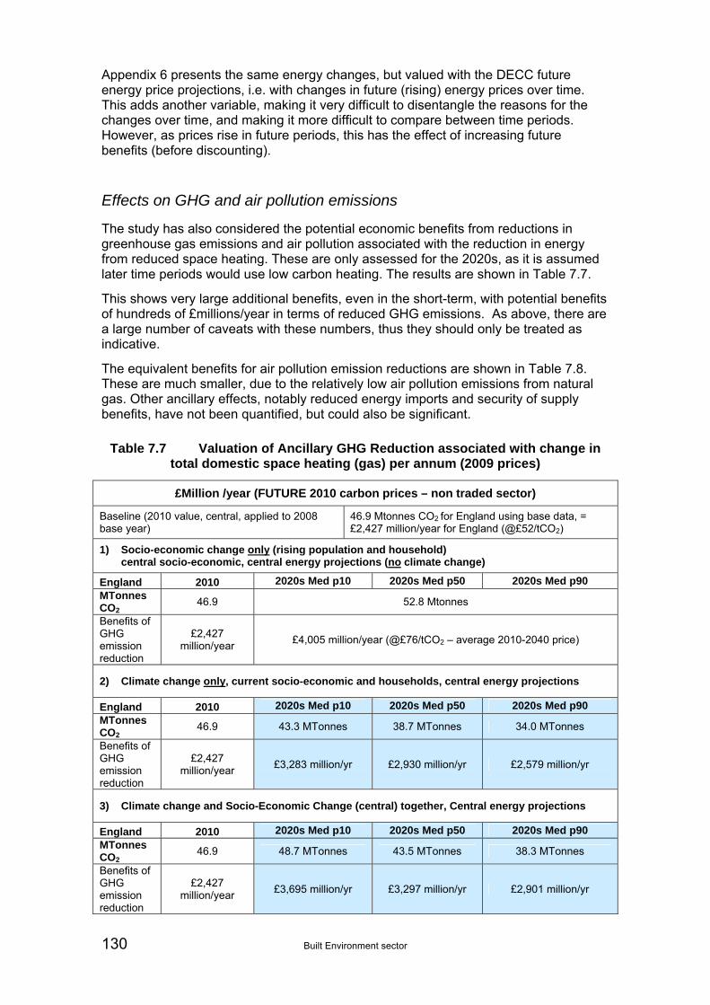
130 Built Environment sector
Appendix 6 presents the same energy changes, but valued with the DECC future energy price projections, i.e. with changes in future (rising) energy prices over time. This adds another variable, making it very difficult to disentangle the reasons for the changes over time, and making it more difficult to compare between time periods. However, as prices rise in future periods, this has the effect of increasing future benefits (before discounting).
Effects on GHG and air pollution emissions
The study has also considered the potential economic benefits from reductions in greenhouse gas emissions and air pollution associated with the reduction in energy from reduced space heating. These are only assessed for the 2020s, as it is assumed later time periods would use low carbon heating. The results are shown in Table 7.7.
This shows very large additional benefits, even in the short-term, with potential benefits of hundreds of £millions/year in terms of reduced GHG emissions. As above, there are a large number of caveats with these numbers, thus they should only be treated as indicative.
The equivalent benefits for air pollution emission reductions are shown in Table 7.8. These are much smaller, due to the relatively low air pollution emissions from natural gas. Other ancillary effects, notably reduced energy imports and security of supply benefits, have not been quantified, but could also be significant.
Table 7.7 Valuation of Ancillary GHG Reduction associated with change in total domestic space heating (gas) per annum (2009 prices)
£Million /year (FUTURE 2010 carbon prices – non traded sector)
Baseline (2010 value, central, applied to 2008 base year)
46.9 Mtonnes CO2 for England using base data, = £2,427 million/year for England (@£52/tCO2)
1) Socio-economic change only (rising population and household) central socio-economic, central energy projections (no climate change)
England 2010 2020s Med p10 2020s Med p50 2020s Med p90 MTonnes CO2
46.9 52.8 Mtonnes
Benefits of GHG emission reduction
£2,427 million/year
£4,005 million/year (@£76/tCO2 – average 2010-2040 price)
2) Climate change only, current socio-economic and households, central energy projections
England 2010 2020s Med p10 2020s Med p50 2020s Med p90 MTonnes CO2
46.9 43.3 MTonnes 38.7 MTonnes 34.0 MTonnes
Benefits of GHG emission reduction
£2,427 million/year
£3,283 million/yr £2,930 million/yr £2,579 million/yr
3) Climate change and Socio-Economic Change (central) together, Central energy projections
England 2010 2020s Med p10 2020s Med p50 2020s Med p90 MTonnes CO2
46.9 48.7 MTonnes 43.5 MTonnes 38.3 MTonnes
Benefits of GHG emission reduction
£2,427 million/year
£3,695 million/yr £3,297 million/yr £2,901 million/yr
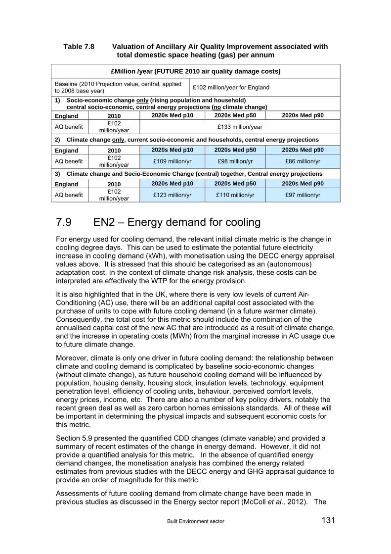
Built Environment sector 131
Table 7.8 Valuation of Ancillary Air Quality Improvement associated with total domestic space heating (gas) per annum
£Million /year (FUTURE 2010 air quality damage costs)
Baseline (2010 Projection value, central, applied to 2008 base year)
£102 million/year for England
1) Socio-economic change only (rising population and household) central socio-economic, central energy projections (no climate change)
England 2010 2020s Med p10 2020s Med p50 2020s Med p90
AQ benefit £102
million/year £133 million/year
2) Climate change only, current socio-economic and households, central energy projections
England 2010 2020s Med p10 2020s Med p50 2020s Med p90
AQ benefit £102
million/year £109 million/yr £98 million/yr £86 million/yr
3) Climate change and Socio-Economic Change (central) together, Central energy projections
England 2010 2020s Med p10 2020s Med p50 2020s Med p90
AQ benefit £102
million/year £123 million/yr £110 million/yr £97 million/yr
7.9 EN2 – Energy demand for cooling
For energy used for cooling demand, the relevant initial climate metric is the change in cooling degree days. This can be used to estimate the potential future electricity increase in cooling demand (kWh), with monetisation using the DECC energy appraisal values above. It is stressed that this should be categorised as an (autonomous) adaptation cost. In the context of climate change risk analysis, these costs can be interpreted are effectively the WTP for the energy provision.
It is also highlighted that in the UK, where there is very low levels of current Air-Conditioning (AC) use, there will be an additional capital cost associated with the purchase of units to cope with future cooling demand (in a future warmer climate). Consequently, the total cost for this metric should include the combination of the annualised capital cost of the new AC that are introduced as a result of climate change, and the increase in operating costs (MWh) from the marginal increase in AC usage due to future climate change.
Moreover, climate is only one driver in future cooling demand: the relationship between climate and cooling demand is complicated by baseline socio-economic changes (without climate change), as future household cooling demand will be influenced by population, housing density, housing stock, insulation levels, technology, equipment penetration level, efficiency of cooling units, behaviour, perceived comfort levels, energy prices, income, etc. There are also a number of key policy drivers, notably the recent green deal as well as zero carbon homes emissions standards. All of these will be important in determining the physical impacts and subsequent economic costs for this metric.
Section 5.9 presented the quantified CDD changes (climate variable) and provided a summary of recent estimates of the change in energy demand. However, it did not provide a quantified analysis for this metric. In the absence of quantified energy demand changes, the monetisation analysis has combined the energy related estimates from previous studies with the DECC energy and GHG appraisal guidance to provide an order of magnitude for this metric.
Assessments of future cooling demand from climate change have been made in previous studies as discussed in the Energy sector report (McColl et al., 2012). The

132 Built Environment sector
projections of increased costs (constant prices, no discounting) are of the order of £13 million to 30 million/year in the 2020s rising to £50 million to £180 million/year in the 2050s, and £250 million to over £1200 million/year by the 2080s. These costs did not capture the likely rise in demand from the additional uptake of AC units or the costs of additional AC units.
For valuation, the estimates above assume the technical costs of generation, based around combined cycle gas cycle as the marginal plant to meet extra demand (around 2.8 pence/kWh). If the more recent DECC energy price guidance values are used (7.4 pence/kWh for domestic and 6.9 p/kWh for commercial, 2010 costs, expressed in 2009 prices) this increases the monetised estimates by more than a factor of two. The resulting costs are therefore in the following ranges: medium costs (£10 – 99 million/year) for the 2020s; high costs (£100 – 999 million/year) for the 2050s and very high costs (>£1 billion/year) for the 2080s.
The results by Day et al. (2009) for London using the current DECC guidance value of 6.8 pence/kWh (2010 commercial costs, expressed in 2009 prices) equates to additional annual costs of £40 to 60 million/year. Using the DECC guidance values with the projected energy prices in 2030 (13 p/kWh) these figures would increase to £80 to 120 million/year. This implies medium costs (£10 – 99 million/year) for the 2020s for London alone (noting London is currently represents around 11% of current cooling demand).
The Pathway Analysis projections do not separate out the marginal effect due to climate change, and are primarily driven by increased wealth. However they do indicate that climate change has the potential to increase energy cooling costs very significantly. Any increase in non-domestic cooling would also add to these values, though the pathway report highlights that these could largely be avoided through a passive response (adaptation).
The results suggest that the monetised values for this metric could be £10 – 99 million/year in 2020s (i.e. a medium ranking), £100 – 1000 million in the 2050s (high), and in excess of £1000 million in the 2080s (very high). Note that these costs are an autonomous adaptation response (i.e. an autonomous adaptation cost).
There are a very large number of caveats associated with these numbers as listed below, and they can therefore only be considered indicative. Nonetheless, given the scale of impacts reported, this is one of the larger economic costs of climate change in the UK, and further modelling work and quantification is warranted for this metric.
Interestingly, the analysis also shows that if this cooling demand is met through electricity use and air conditioning, the monetised GHG and air quality impacts are likely to be significant. It is likely that current mitigation policy would reduce these costs very significantly even for the 2020s, and may entirely remove them in later time periods (2050s and 2080s).
A number of important caveats are associated with these indicative values.
The scoping analysis does not take account of any urban heat island effects. This may mean there is the potential to underestimate the cooling demand.
The analysis does not take into account the costs of cooling appliances.
The analysis does fully not take account of efficiency improvements or technological change in cooling appliances, or improved energy efficiency of the housing stock.
The analysis does not include policy relating to insulation of existing housing stock or zero carbon homes emissions standards.
Built Environment sector 133
The analysis does not consider how prices would change with future global emissions scenarios.
The analysis does not fully account for the changes in the energy mix for supplying residential cooling and the UK’s short- and long-term (2050) greenhouse gas emissions target.
A number of other key issues and cross sector linkages are highlighted. First, there may be additional cooling demand in the industrial and transport sectors, though the latter is considered in the Transport sector report (Thornes et al., 2012). Second, there are benefits of reduced space heating demand (metric BE9) that offset the energy impacts of increased cooling.
There are also cross sector linkages with non-residential building overheating (metric BE3), which overlap with cooling demand increases, because if there is cooling this will reduce the lost productivity and residential over-heating. There is therefore a risk of double counting if cooling demand and BE3 are added together. Similarly there is a risk of double counting between temperature-related (heat) mortality and morbidity (HE1, excess mortality, based on daily mean temperature and population) as air conditioning may reduce health impacts from heat.
7.10 WA5 – Water supply-demand deficit
In the first instance the welfare value of water in the supply-demand context is approximated by the use of supply-side cost data. Data provided in Walker and Burgess (2007) suggest a range of marginal cost estimates at the national level of between £0.1m/Ml/day and £7m/Ml/day, with a central (median) value of £2m/Ml/day. These costs comprise of both capital and operating cost components. It should be noted that whilst Walker and Burgess (2007) highlight considerable regional, sectoral and other location-specific variation, the range presented is intended to reflect much of this variation. This range is also equivalent to that reported in the National Ecosystem Assessment (NEA) though the NEA uses a different metric (£/m3).
The range of values identified above comprise of present values over the lifetime of the different supply-side options considered. For this analysis, it is more useful to express these costs in annualised terms. The assumption made in Mott MacDonald (1998) that the lifetime is 40 years is adopted. Thus, crudely, the central value is £0.05 million Ml/day annually. Applying the central value, only, the monetary values of the deficits (surpluses) are presented in Tables 7.9 and 7.10.
Under current population and ONS population projections respectively, Tables 7.9 and 7.10 present the monetised cost of the water supply-demand surplus and deficits across the three time periods to the end of this century, and under the three UKCP09 climate change scenarios. The totals shown as negative values denote water balance deficits, whilst the positive values denote surpluses compared to the present period. Some clarifications should be made with regard to the interpretation of these results. First, positive values (that feature primarily in the earlier time periods) should not necessarily be interpreted to mean that these totals constitute welfare benefits to the UK. Whilst there may be resource advantages to be obtained, for example, from capturing some of the additional winter rainfall in reservoirs rather than having to institute effluent re-use or desalinisation schemes to meet summer deficits, current water infrastructure is designed to operate optimally under present climatic patterns, i.e. with current precipitation levels. It is therefore unlikely to be able to fully exploit the benefits of increased winter rainfall.
Table 7.9, which reports the monetisation for climate change alone (on current socio-economic scenarios), shows that the surplus balances that are a feature of the p10 and

134 Built Environment sector
p50 climate scenarios in the 2020s turn to deficits by the 2080s, where they range from an annual deficit of £11m in the 10% probability level of the low emissions climate scenario to £338m in the 90% probability level of the high emissions climate scenario. The results for the 50% probability level under the Medium emissions scenario are £12m, minus £141m and minus £241m per annum for the 2020s, 2050s and 2080s time periods respectively.
Table 7.10, which includes climate change and socio-economic change, reflects a similar pattern as Table 7.9. However, the results in Table 7.10 with higher future population projections exacerbate the deficit estimates and reduce the surpluses estimated. Indeed, apart from the results for the 10% probability level under the climate scenarios in the 2020s time period, which remain in surplus, there are now deficits under all scenarios in all three time periods. The sizes of the deficits are significantly larger and equate to a factor of two under the 50% probability level for the 2080s time period and are over £200m per year in absolute terms.
Table 7.9 Annual water supply-demand balance in the UK – marginal climate change impacts on Deployable Outputs
£million/year, 2010 prices, no uplift, no discounting; current population; 150 l/h/d per capita consumption
Climate change only
Climate change scenario Low
Emissions Medium
Emissions High
Emissions
p10 108 114 109
p50 11 12 10 2020s
p90 -97 -102 -97
p10 36 6 -26
p50 -106 -141 -174 2050s
p90 -245 -282 -296
p10 -11 -86 -124
p50 -166 -212 -229 2080s p90 -296 -317 -338
Table 7.10 Annual water supply-demand balance in the UK considering climate change impacts and socio-economic change (population) on Deployable
Outputs £million/year, 2010 prices, no uplift, no discounting; Baseline (ONS) population projections; 150 l/h/d per
capita consumption
Socio-economic scenario Climate change and population
change (baseline scenario)
Climate change scenario Low
Emissions Medium
EmissionsHigh
Emissions
p10 50 56 50
p50 -46 -46 -46 2020s
p90 -155 -161 -156
p10 -94 -123 -156
p50 -239 -275 -310 2050s
p90 -382 -421 -437
p10 -204 -282 -323
p50 -366 -416 -437 2080s p90 -503 -530 -557
Regional breakdowns of these results are available in the Water sector report (Rance et al., 2012).

Built Environment sector 135
7.11 WA6 - Population affected by a water supply-demand deficit
WA5 utilised the cost of supply to proxy for the welfare value, based on the assumption that the two would equate in the long run. Since the current metric expresses the same climate change risk, water supply-demand balance, though in a different form, the supply cost measure is relevant here since it represents the cost of preventing supply-demand deficits and, by extension, the affected population. Consequently, there is a strong risk of double-counting if this metric is monetised.
WA6 does not provide quantitative estimates of the additional risks relating to non-connected households and business, or the amount that businesses may be willing to pay above that of the supply cost. As a result, it is not possible to make quantitative estimates of the welfare costs associated with these risks. As a consequence, an informed judgement has been made as to the potential order of magnitude that this risk metric implies, additional to the costs estimated in WA5. It is judged that since these two groups of water consumers may be sizeable, the risk across the UK could be Medium (£10m - £99m, annually).
7.12 Flooding costs
The monetary estimates are made within the flood model described in the Floods and Coastal Erosion sector report. The values used are consistent with those recommended for use in the Defra/Environment Agency Flood and Coastal Erosion Risk Management Appraisal Guidance. Flood defence levels are assumed to be kept constant in absolute terms; thus, under climate change scenarios the relative risk levels will increase. No additional autonomous adaptation, for example by household or in household design, is assumed.
The EAD results are outlined in Section 5 of this report and the Floods and Coastal Erosion sector report and are not repeated here. However, in order to facilitate results in other sectors, Table 7.11 utilises the results to derive the EADs attributable to climate change alone, for the p50 Medium emissions climate scenario for England and Wales. These results are generated on the basis that flood defences are maintained to present standards. The residential totals are further disaggregated to indicate that whilst approximately 75% of the cost will be borne by household insurance companies, one quarter of the total is attributed to provision of emergency and hospital services (see e.g. Chatterton et al., 2009).
Table 7.11 Property flooding: Climate attributable EADs – England and Wales £m, 2010, no uplift or discounting; p50 Medium emissions climate scenario; No socio-economic change.
Residential Total
Insurance NationalNon-
residential
2020s 345 115 440 910 2050s 720 240 790 1760 2080s 1095 365 1090 2550
7.13 HE1 – Temperature mortality (Heat)
Valuation of mortality (or fatality) focuses solely on the disutility welfare component; specifically the valuation of changes in the risk of death in a given time period. This is commonly expressed through the metric of a Value of a Prevented Fatality (VPF), also
136 Built Environment sector
known as the Value of a Statistical Life (VSL). These metrics are already widely used in Government appraisal and cost-benefit analysis, for example in transport appraisal. An alternative metric, the Value of a Life Year (VOLY), is also suggested for use in contexts such as air quality regulatory impact analysis where it is likely that the shortening of life time associated with a change in mortality risk is thought to be relatively small (IGCB, 2007). It is stressed that there is some debate in the literature as to the relative merits of these two metrics. Current best practice is been to use both metrics, at least in sensitivity analysis.
The search for appropriate unit values relies on the available literature. Since there are no values currently recommended for use in Government guidance for the climate change context, unit values have been transferred.
The most relevant context would appear to be that of air quality regulation, in which the Interdepartmental Group on Costs and Benefits (IGCB, 2010) has made recommendations on the appropriate unit values to apply. This guidance is particularly relevant, given guidance that it is important that the length of life time should be material in the valuation of mortality impacts34. The IGCB suggests a VOLY-equivalent of £60,00035. In order to incorporate length of life time into the monetary estimates it has been assumed that each additional death is associated with a loss of four months – the mid-point of a suggested range of two to six months36.
It is stressed that the results are based on the physical impact estimates provided earlier in this sectoral report. A number of important issues are associated with these estimates and these should be considered in interpreting the estimates below. The numbers below do not include physiological acclimatisation (a form of autonomous adaptation), i.e. the fact that future population will naturally adjust to future higher temperatures. It is highlighted that previous studies that have included this adjustment (Kovats et al., 2006 and Watkiss et al., 2009) derive very much lower estimates of physical and economic impacts. However, it is also highlighted that the climate change data used does not account for elevated temperatures in urban areas, i.e. from any urban heat island effects, and therefore may underestimate effects, particularly in major cities. It is also stressed that there are more complex issues in the acclimatisation, lag phases, etc that may mean that heat and cold related effects need to be treated differently, in terms of quantification and valuation. The results also do not account for other socio-economic factors (e.g. income growth, age profile or age specific mortality rates) that might affect relative risks.
There are some cross-sectoral linkages that affect these results and that are important when aggregating risks between sectors. The most important of these is the increased cooling demand and energy use in the built environment and energy analysis. The assumption of ownership and usage of air conditioning significantly reduces the effects of temperature on health outcomes to heat (Ostro et al., 2010) and would thus be expected to reduce the estimated risks.
The results are presented in Tables 7.12 – 7.16.
Table 7.12 shows the monetary value of additional mortality impacts under the three climate scenarios, given current population, i.e. in the absence of future socio-economic change. No acclimatisation or increased adoption of air conditioning is assumed. Tables 7.14 - 7.16 show equivalent results under low, principal and high population projections, i.e. combining future climate and future socio-economic change. It is stressed that these combined effects are not due only to climate change alone.
34 John Henderson, Department of Health, personal communication
35 Noise & Health – Valuing the Human Health Impacts of Environmental Noise Exposure” The Second Report of the IGCB(N)
36 Dr Sotiris Vardoulakis, Health Protection Agency and sectoral report author, personal communication

Built Environment sector 137
Table 7.13 presents the monetary totals for the English Regions and the DAs, for the Medium emissions climate scenario and principal population projection.
It is clear from Table 7.12 that as climate change develops over the course of the century the size of the heat-related mortality risks increase significantly, so that the increased welfare cost in the 2080s is at least five-six times higher than that in the 2020s, whilst doubling between the 2050s and 2080s. Contrasting Tables 7.12 and 7.14 - 7.16, it is apparent that the different population projections have a smaller effect on the scale of the results compared with the impact of climate change across the time periods.
Table 7.12 Valuation of Life Years Lost (heat) per year for the UK for the different emissions scenarios
£m, annual, 2010 prices; current population; baseline period 1993-2006; no acclimatisation
2020 2050 2080 Scenario
p10 p50 p90 p10 p50 p90 p10 p50 p90
Low 25 54 102 37 79 157
Medium 13 28 51 32 65 125 53 115 233
High 38 78 150 80 172 347
Table 7.13 Valuation of Life Years Lost (heat) per year for the English regions for the medium emissions scenario
£m, annual, 2010 prices; principal population; baseline period 1993-2006; no acclimatisation
2020 2050 2080
Administrative Region p10 p50 p90 p10 p50 p90 p10 p50 p90
South West 1.3 2.8 5.1 4.1 8.5 16.9 7.8 17.3 36.3
South East 2.1 4.6 8.4 6.7 14.1 26.8 13.1 28.3 56.3
London 2.3 4.7 8.4 6.9 14.0 26.5 13.1 28.1 55.9
East of England 1.9 4.2 7.5 5.9 11.8 21.9 11.3 23.6 46.4
West Midlands 1.4 3.2 5.9 4.0 8.2 16.1 7.4 15.9 33.4
East Midlands 1.1 2.3 4.1 3.0 5.9 10.9 5.6 11.6 22.9
North West 1.4 3.1 5.7 3.1 6.6 12.8 5.5 12.4 25.7
North East 0.4 0.9 1.7 1.0 2.1 4.0 1.8 4.0 8.1
Yorkshire and Humber 1.1 2.4 4.2 2.8 5.5 10.2 5.2 10.8 21.6
England 12.9 28.2 51.1 37.5 76.7 146.1 70.8 152.0 306.4

138 Built Environment sector
Table 7.14 Valuation of Life Years Lost (heat) per year for the UK for the different emissions scenarios: low population
£m, annual, 2010 prices; baseline period 1993-2006; no acclimatisation
2020 2050 2080 Scenario
p10 p50 p90 p10 p50 p90 p10 p50 p90
Low 27 58 112 38 83 163
Medium 14 30 55 35 71 136 56 120 243
High 42 85 164 83 179 362
Table 7.15 Valuation of Life Years Lost (heat) per year for the UK for the different emissions scenarios: principal population
£m, annual, 2010 prices; baseline period 1993-2006; no acclimatisation
2020 2050 2080 Scenario
p10 p50 p90 p10 p50 p90 p10 p50 p90
Low 30 64 123 51 110 218
Medium 14 31 57 41 84 161 77 165 334
High 46 94 180 111 239 482
Table 7.16 Valuation of Life Years Lost (heat) per year for the UK for the different emissions scenarios: high population
£m, annual, 2010 prices; baseline period 1993-2006; no acclimatisation
2020 2050 2080 Scenario
p10 p50 p90 p10 p50 p90 p10 p50 p90
Low 38 80 153 69 149 295
Medium 15 33 60 48 98 187 101 217 438
High 57 117 224 150 324 651
A sensitivity using VSL estimates (a value of £1.79m, as used by Department for Transport) is presented in Table 7.17 for the UK level analysis, where no socio-economic (population) change is included. Thus, apart from the valuation metric, it is equivalent to Table 7.12 above. Clearly, the results in Table 7.17 are much higher than the earlier table.
Table 7.17 Valuation of premature fatalities (heat) per year for the UK for the different emissions scenarios: current population
£m, annual, 2010 prices; baseline period 1993-2006; no acclimatisation
2020s 2050s 2080s Scenario
p10 p50 p90 P10 p50 p90 p10 p50 p90
Low 1036 3110 6878 1862 5074 11173Medium 230 1280 2990 1517 3994 8648 3108 7897 17084High 1988 4991 10604 5108 12332 25785

Built Environment sector 139
7.14 HE2 – Temperature morbidity (heat)
Previous economic analysis in UK Government in the context of air quality regulation has assessed the economic costs of hospital admissions (IGCB, 2007). This assumes that hospital admissions (HA), whether resulting from respiratory or cardio-vascular illness, are valued equivalently.
Based on Department of Health (1999), IGCB (2007) estimates the total resource cost, and per patient-day of an HA to be £2,423 and £266 respectively (2010 prices). In its central estimates, IGCB (2007) assumes that since most respiratory hospital admissions (RHAs) are borne by the retired population, no productivity losses and associated costs are incurred as a result of RHAs. In accordance with IGCB recommendations, total WTP for HA patient-days is then assumed to be £625 (£350 and £900 constitute lower and upper bounds around this central estimate) at 2010 prices.
It is stressed that the numbers below use the physical impact estimates provided earlier in this chapter. A number of important issues are associated with these estimates, as reported in the earlier analysis, and these should be considered in interpreting the estimates below. Further, the issues raised in relation to HE1 above, notably the urban temperature effects and other socio-economic factors including age profile, and the cross-sectoral overlap with cooling are highlighted.
Tables 7.18 and 7.19 present the monetary results for heat-related morbidity using current population as the baseline (climate change only), and the three population projections (i.e. with climate change and future socio-economic change) respectively. No acclimatisation is assumed.
When comparing the two tables, as with HE1, it is clear that climate change, rather than socio-economic change, accounts for the majority of the additional cost of morbidity. Across the population projections, the uncertainty appears to increase in the furthest time period, where the result for the High emissions scenario is approximately double that for the Low emissions scenario.
Table 7.18 Monetary value of annual additional patient days in UK per year due to increased temperatures: current population – tentative estimates
£m, annual, 2010 prices; baseline period 1993-2006
Emissions scenario (p50)
2020s 2050s 2080s
Low 111 181
Medium 46 142 281
High 178 439

140 Built Environment sector
Table 7.19 Monetary value of annual additional patient days in UK per year due to increased temperatures: population projections – indicative estimates
£m, annual, 2010 prices; baseline period 1993-2006
Population projection
Emissions scenario (p50)
2020s 2050s 2080s
Low 121 188
Medium 49 156 294
Low
High 194 459
Low 134 252
Medium 51 183 404
Principal
High 215 612
Low 166 340
Medium 54 213 530
High
High 266 828
7.15 HE3 – Flood related deaths
The metric to be valued is the number of fatalities resulting from floods. Thus, the VPF (VSL) is the relevant monetary metric. The UK Department of Transport uses a VPF in its economic appraisal of accident fatalities in the UK. As documented in unit 3.4.1 of webtag (http://www.dft.gov.uk/webtag/), this value is currently £1.79m (2010 prices). It is highlighted that this assumes the values are readily transferable to the floods context, which does involve a number of important contextual differences, not least the involuntary risk, as well as the size of the risk change. The value that is currently quoted in Defra guidance is £1.49m37. This latter value is therefore adopted in this analysis.
The monetary totals for climate-induced flood related deaths are presented in Tables 7.20 and 7.21. Whilst Table 7.20 shows the results using current population (i.e. climate change only on current conditions), those in Table 7.21are based on a range of population projections, and thus include the effects of climate change and socio-economic change. The results are presented for a range of climate scenarios and distributions, depending on the time period.
In both tables, the number - and welfare cost - of fatalities increases further into the future, and across the climate scenarios from low to high. As with HE1, the climate signal is more important than the population signal in determining the size of the additional cost. It is also notable that the range of uncertainty expressed by the results across the probability distribution function (p10 - p90) within a given emissions scenario is substantial, the latter being a factor of four greater than the former in the 2020s.
37 Defra (2008) Defra Flood and Coastal Defence Appraisal Guidance: Social Appraisal Supplementary Note to Operating Authorities: Assessing and Valuing the Risk to Life from Flooding for Use in Appraisal of Risk Management Measures. May 2008

Built Environment sector 141
Table 7.20 Monetary value of annual additional flood related deaths per year due to extreme event flooding and storms: future climate change
£m, 2010 prices; current population
2020s 2050s 2080s Med. Med. Med. Low Low Med. High High Low Low Med. High High
p10 p50 p90 p10 p50 p50 p50 p90 p10 p50 p50 p50 p90
6 17 25 9 26 31 35 51 20 39 47 57 103
Table 7.21 Monetary value of annual additional flood related deaths per year due to extreme event flooding and storms: future climate and population change
£m, 2010 prices; future socio-economic change (population projections)
2020s 2050s 2080s Med. Med. Med. Low Low Med. High High Low Low Med. High High
Population projection
p10 p50 p90 p10 p50 p50 p50 p90 p10 p50 p50 p50 p90
Low 8 20 28 12 30 35 39 55 21 41 49 60 106
Principal 9 21 30 16 37 42 47 64 33 57 66 77 125
High 10 23 32 21 44 50 55 73 47 76 85 97 146
7.16 HE5 – Temperature mortality (cold)
The method used to estimate the monetary value of mortality avoided is the same as that adopted in HE1. Hence, the number of premature deaths is converted to life years. In this case each death is assumed to result in a loss of lifetime of six months and the unit value of VOLY of £33,800 (2010 prices) is then applied, as recommended in IGCB (2007).
The results are presented in Tables 7.22 to 7.26. Table 7.22 shows the monetary value of additional mortality impacts under the three climate scenarios, given current population (i.e. climate change only). Tables 7.24 - 7.26 show equivalent results under low, principal and high population projections, i.e. with future climate and socio-economic change. Table 7.23 presents the monetary totals for the English Regions and the Devolved Administrations, for the Medium emissions climate scenario and principal population projection. No acclimatisation is assumed.
It is clear from Table 7.22 that as climate change develops over the course of the century the size of the cold-related mortality benefits increase significantly, so that the welfare cost in the 2080s is approximately three times higher than that in the 2020s. Contrasting Tables 7.22 and 7.24 -7.26, it is apparent that the different population projections have a small effect on the scale of the results compared with the impact of climate change across the time periods. It is also notable that the range of uncertainty expressed by the results across the probability distribution function (p10-p90) within a given emissions scenario is substantial, the latter being at least a factor of two greater than the former in each of the three time periods. Ranges are given in the values for each scenario owing to uncertainty over the relevant temperature thresholds that could cause death.
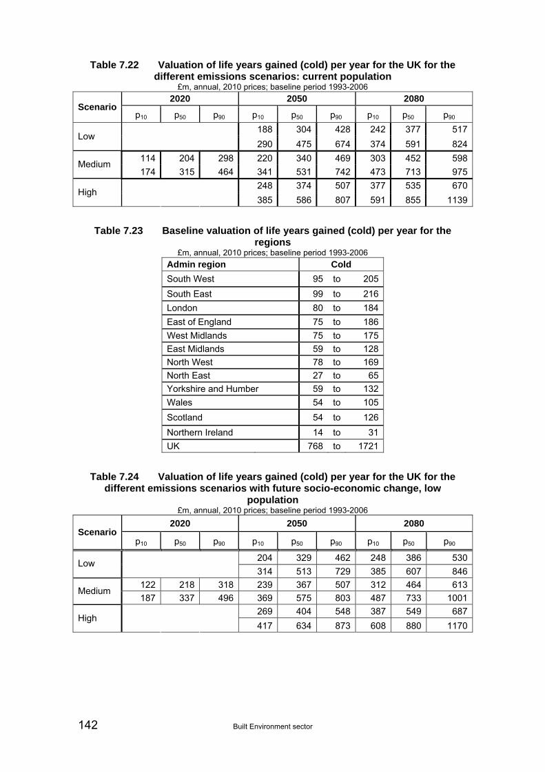
142 Built Environment sector
Table 7.22 Valuation of life years gained (cold) per year for the UK for the different emissions scenarios: current population
£m, annual, 2010 prices; baseline period 1993-2006
2020 2050 2080 Scenario
p10 p50 p90 p10 p50 p90 p10 p50 p90
188 304 428 242 377 517Low
290 475 674 374 591 824
114 204 298 220 340 469 303 452 598Medium
174 315 464 341 531 742 473 713 975
248 374 507 377 535 670High
385 586 807 591 855 1139
Table 7.23 Baseline valuation of life years gained (cold) per year for the regions
£m, annual, 2010 prices; baseline period 1993-2006
Admin region Cold
South West 95 to 205
South East 99 to 216
London 80 to 184
East of England 75 to 186
West Midlands 75 to 175
East Midlands 59 to 128
North West 78 to 169
North East 27 to 65
Yorkshire and Humber 59 to 132
Wales 54 to 105
Scotland 54 to 126
Northern Ireland 14 to 31
UK 768 to 1721
Table 7.24 Valuation of life years gained (cold) per year for the UK for the different emissions scenarios with future socio-economic change, low
population £m, annual, 2010 prices; baseline period 1993-2006
2020 2050 2080 Scenario
p10 p50 p90 p10 p50 p90 p10 p50 p90
204 329 462 248 386 530Low
314 513 729 385 607 846
122 218 318 239 367 507 312 464 613Medium
187 337 496 369 575 803 487 733 1001
269 404 548 387 549 687High
417 634 873 608 880 1170

Built Environment sector 143
Table 7.25 Valuation of life years gained (cold) per year for the UK for the different emissions scenarios with future socio-economic change, principal
population £m, annual, 2010 prices; baseline period 1993-2006
2020 2050 2080 Scenario
p10 p50 p90 p10 P50 p90 p10 p50 p90
240 388 545 341 531 729Low
370 605 859 529 834 1163
130 234 341 297 390 538 463 518 686Medium
200 362 532 391 609 851 543 818 1118
317 477 646 533 755 945High
491 748 1029 836 1209 1608
Table 7.26 Valuation of life years gained (cold) per year for the UK for the different emissions scenarios with future socio-economic change, high
population £m, annual, 2010 prices; baseline period 1993-2006
2020 2050 2080 Scenario
p10 p50 p90 p10 P50 p90 p10 p50 p90
279 450 633 447 697 955Low
430 703 997 694 1094 1524
133 239 348 327 503 694 562 836 1105Medium
204 369 542 506 787 1098 878 1321 1804
368 553 750 698 990 1239High
570 868 1194 1096 1585 2108
7.17 BU6 – Increased exposure for mortgage lenders
This metric is concerned with the impact of increasing flood risk on mortgage lending revenues as a function of market changes and the important issue of asset devaluation in the event of the loss of insurance cover.
For the purposes of this analysis, the number of properties at significant risk of flooding (coastal and fluvial) is used as an indicator of the impact of flooding on the availability of insurance, and consequently on the level of mortgage lending exposed. Here, the baseline (current) sea level and river flow peak data are used to derive the existing level of significant risk to properties in different regions (by numbers of properties).
As discussed in Section 5.16, it is projected that the value of mortgages that could be affected by this risk is of the order of £1 billion to £8 billion by the 2050s rising to £2 billion to £9 billion by the 2080s (at today’s prices).
This risk metric is not concerned with a welfare impact per se; the related welfare impact i.e. flooding to residential property is presented in the Floods and Coastal Erosion sector report, risk metric FL6. Rather it is concerned with the scale of the mortgage fund value at risk, relative to the 2008 baseline. The values given are total asset values and are therefore not comparable to results presented elsewhere in the risk assessment in annual terms.

144 Built Environment sector
7.18 BU10 – Loss of staff hours due to high internal building temperatures
In the specific case of cooling requirements, longer, drier summer periods may cause overheating in naturally ventilated buildings and affect the capacity of low energy cooling systems to provide comfortable conditions across all building types. These changes may have knock-on implications for worker health and safety, productivity and product quality.
Metric BE3 (overheating of buildings) considered the number of days a year when the temperature exceeds a comfort level taken as the threshold for overheating. The monetisation of this metric in Section 7.6 considered the potential effects on productivity, and is therefore essentially the same as this metric.
It is also noted that there may be some productivity gains from climate change in relation to lost time at work, travel time, etc. from the reduction in colder temperatures, although these have not been considered.
This risk metric is concerned with the scale of the productivity losses associated with overheating in buildings. The results, expressed in terms of turnover, were given in Section 5.17, adjusted to identify the climate attributable impacts net of the baseline. The lack of detailed economic analysis in this assessment leads to some questions over the reliability of these estimates. Whilst they are retained here, this is an important area for future investigation.
With climate change, the estimated number of days above the temperature threshold rises significantly, particularly in the South-East and London, and especially in the later time periods (2080s). In the absence of any action, this would lead to potentially high costs, from reduced productivity and lost work time, which could plausibly be of the order of hundreds of millions or even billions of pounds annually by later time periods, given the size of the working population potential impacted (35 million in the UK) combined with the unit value of a day of lost productivity (£150/day on average). These are therefore given a high to very high rating.
However, particularly care is needed in interpreting these changes, because of the private sector autonomous response to climate change. In the face of rising temperatures, companies may adjust the working environment to avoid falls in productivity and in direct response to occupational health legislation/guidance that may be provided in future. The indicative results above may therefore be an over-estimate of the actual costs likely to occur.
There are cross-sectoral linkages with energy cooling costs, both in the current and future stock of office buildings over time (including retrofit and refurbishment cycles). As highlighted above, adding energy cooling costs to these productivity costs will involve double counting (as there will either be the former or the latter, but not both together).

Built Environment sector 145
8 Adaptive Capacity
8.1 Overview
Adaptive capacity considers the ability of a system to design or implement effective adaptation strategies to adjust to information about potential climate change, to moderate potential damages, to take advantage of opportunities, or to cope with the consequences (Ballard, 2009, after IPCC, 2007). This can be considered as having two components; the inherent biological and ecological adaptive capacity of ecosystems and the socio-economic factors determining the ability to implement planned adaptation measures (Lindner et al., 2010). Considering adaptive capacity is essential for adaptation planning and the CCRA project has included work in this area that will contribute to the ongoing Economics of Climate Resilience study and the National Adaptation Programme. The CCRA work on adaptive capacity focuses on structural and organisational adaptive capacity and this chapter provides an overview of the assessment approach. The subsequent sections of this chapter provide an overview of the findings from other work on adaptive capacity in the Built Environment sector that has been carried out.
The climate change risks for any sector can only be fully understood by taking into account that sector’s level of adaptive capacity. Climate change risks can be reduced or worsened depending on how well we recognise and prepare for them. The consequences of climate change are not limited to its direct impacts. Social and physical infrastructure, the backdrop against which climate change occurs, must also be considered. If such infrastructure is maladapted, the economic, social or environmental cost of climate impacts may be much greater; other consequences could also be considerably more detrimental than they otherwise might have been. Avoiding maladaptation is one outcome of high adaptive capacity; high adaptive capacity lowers the negative consequence of climate impacts. Conversely, low adaptive capacity increases the negative consequences.
8.2 Assessing structural and organisational adaptive capacity
The methods used for assessing structural and organisational adaptive capacity in the CCRA are based on the PACT framework38. The work included a preliminary literature- and expert interview-based assessment of all eleven sectors in the CCRA. This was followed by more detailed analysis for the following sectors:
Business, Industry and Services (focusing on the finance sector)
Transport (focusing on road and rail)
Built Environment (focusing on house building)
Health
Biodiversity and Ecosystem Services
Water 38 PACT was developed in the UK as one of the outcomes of the ESPACE Project (European Spatial Planning: Adapting to Climate Events) http://www.pact.co/home.
146 Built Environment sector
Structural adaptive capacity
The extent to which a system is free of structural barriers to change that makes it hard to devise and implement effective adaptation strategies to prepare for future impacts. This covers issues such as:
Decision timescales: This considers the lifetimes of decisions, from their conception to the point when their effects are no longer felt. The longer this period is, the greater the uncertainty as to the effects of climate change impacts. Cost-effective adaptation becomes harder. Potential climate impacts also become more extreme over longer timescales. This means that a greater scale of adaptation may need to be considered, and that the barriers to adaptation resulting from 'lock-in' to maladapted processes become more pronounced (Stafford-Smith et al., 2011). Adaptive capacity is therefore lower, and maladaptation more likely, when long-lasting decisions are taken.
Activity levels: This considers what opportunities are there for adaptation, and on what scale. The frequency with which assets are replaced or created determines how many opportunities there will be to take action which increases adaptive capacity.39 In addition, when a lot of asset replacement and/or new investment is expected, there will be more chances to learn from experience, which increases adaptive capacity.
Maladaptation: This evaluates the effect of decisions already made on adaptive capacity. Long-term previous decisions which have reduced adaptive capacity are often difficult or expensive to reverse. Such decisions were made either before climate change was recognised as an issue, or more recently as a result of poor organisational capacity. Such maladaptation makes implementing effective strategies much harder.
Sector (or industry) complexity: This refers to the level of interaction between stakeholders within an industry, or with outside industries and groups, that is required to facilitate effective decision-making. Complexity is higher (and adaptive capacity lower) when many stakeholders are involved in decision-making and when their agendas (e.g. their financial interests) differ substantially.
Organisational adaptive capacity
Organisational adaptive capacity is the extent to which human capacity has developed to enable organisations to devise and implement effective adaptation strategies. Effective adaptation requires decision-making that takes account of an uncertain future and avoids locking-out future options that might be more cost-effective if climate impacts become more severe, or arrive more rapidly, than expected. The PACT framework used to assess this recognises different levels of adaptation. This framework is arranged in a hierarchy of ‘Response Levels’ (‘RLs’), as set out below, of increasing capacity40. These levels do not supersede one another; instead, each one builds on the experiences and practices built up in the previous response level. Organisations may need to be active on all levels for an effective adaptation programme. An RL4 organisation focused on breakthrough projects still needs to be stakeholder-responsive, for example.
RL1: Core Business Focused: At this level, organisations see no benefit from adapting; if change is required of them, it should both be very
39This differs from ‘Decision timescales’ because investment in a sector is not continuous but varies over time, with periods of high investment being followed by periods of little or no investment.
40 The PACT framework contains six response levels: those cited are the most relevant to the adaptation field.
Built Environment sector 147
straightforward to implement and also incentivised, e.g. through ‘carrots’ and ‘sticks’.
RL2: Stakeholder Responsive: At early stages of adaptation, organisations lack basic skills, information, processes and also skilled people; they need very clear advice and information plus regulations that are straightforward enough to help them get started.
RL3: Efficient Management: As organisations begin to professionalise adaptation, they become more self-directing, able to handle short term impacts up to 10 years (Stafford-Smith et al., 2011). They need professional networks, best practice guidelines, management standards, etc.
RL4: Breakthrough projects: When impacts beyond 10 years need to be considered, organisations may need to consider more radical adaptation options. As well as high quality support from scientists, they may need support with the costs of innovation.
RL5: Strategic Resilience: Adapting a whole region or industry for long-term climate impacts of 30 years or more requires lead organisations to develop very advanced capacity that is able to co-ordinate and support action by a wide range of actors over programmes that are likely to last for many years.
8.3 Adaptation Sub-Committee Reports The first Adaptation Sub-Committee (ASC) Progress Report (ASC, 2010) considered the steps the UK should be taking to adapt to climate change, as well as what progress has been made so far and what further action is required. It identified a number of priority areas for early action, including land-use planning and designing and renovating buildings. Findings for these two priority areas relevant to the Built Environment sector were reported in the second progress report (ASC, 2011) and are summarised here.
8.3.1 Land-Use Planning
The ASC (2011) concluded that the land use planning faces difficult trade-offs in assessing climate change considerations against other, shorter-term priorities. Their findings suggest that there is limited evidence that local authorities are taking into account long-term costs when making decisions on the strategic location of new development in their Local Plan. The report suggests that a strategic approach is needed to manage vulnerability at community and individual property scale. This would involve weighing up the long-term costs of climate impacts against more immediate social and economic benefits from development. There may be a role for developing localised indicators that allow communities to understand how development decisions are affecting their vulnerability to climate risks.
The ASC (2011) analysis showed variable uptake of adaptation measures at the property level in development applications. Nearly all applications in areas of river and coastal flood risk included adaptation and around half the applications in areas of surface water flooding risk included adaptation. Other climate risks, for example heat stress, are not as widely considered within development applications.

148 Built Environment sector
8.3.2 Designing and Renovating Buildings
The ASC (2011) identified buildings as a priority area for adaptation, because decisions concerning the design, construction and renovation of buildings are long lasting and potentially costly to reverse. An in-depth, quantitative assessment of preparedness in the residential buildings sector was undertaken and a range of adaptation measures at the individual property level evaluated. A number of low-regret adaptation options were identified to protect against water stress, flooding and heat stress.
The Government has taken some action to address the climate risks facing the residential built environment sector. Generally this action has tended to focus on new developments. In the boroughs surveyed, uptake is higher for flood resilience and water saving measures than for measures to reduce the risk of overheating (without resorting to air-conditioning).
Limited evidence was found on the uptake of adaptation measures in existing homes, where there is less regulation. This is especially true for property level measures to reduce the risk of heat stress.
A number of barriers prevent the uptake of low-regret measures across the sector. Sufficient incentives are required for householders to take action. Information on climate risks, options for managing risks and professional advice on the installation of measures also needs to be more readily available to reduce any hidden costs that householders and developers may incur.
8.4 Summary The ASC analysis focused on the housing/residential sector. A means of assessing adaptive capacity in a more general context, is provided by results of the Carbon Disclosure Project (CDP) survey, 2008. This gave some information on the extent to which business organisations have begun the process of adaptation. The focus was on early stage adaptation activities rather than on the much more sophisticated adaptation activities that would be required, for instance at a period of major investment in long-lasting assets. This means that low scores indicate with relatively high confidence that adaptation activity is absent, but that relatively high scores do not necessarily indicate that adaptation activities are sufficient, or even necessarily very far developed. This survey suggested that the status of adaptation actions is low in real estate (management and house building) and real estate (leisure).
Expert stakeholders consulted during the early stages of the CCRA project expressed the view that the adaptive capacity of the Built Environment sector is low (Capon, 2010). In building projects, capital cost and mandatory standards imposed by regulation are often the most important drivers for decision-making. Capital versus life-cycle cost of a project is rarely considered. For many stakeholders, the issue of climate change lies too far into the future to trigger investment in the current economic climate. Thus the driver of capital cost has a major impact on the degree of adaptation that is currently achieved.
Notwithstanding these obstacles, a sound business case can be made for including adaptation in building design now (Gething, 2010). Companies which position themselves as the first movers in developing and testing adaptation strategies for new and existing buildings should have a significant competitive advantage in the future.
In light of the need to build adaptive capacity within the sector, the Technology Strategy Board has launched the “Design for Future Climate” competition, which is to invest £5m in designing strategies for climate change adaptation for new and existing buildings.

Built Environment sector 149
9 Discussion A number of key risks to the Built Environment sector have been analysed within the CCRA. This section discusses the outcomes, with risks grouped thematically rather than in strict numerical order. Gaps and limitations in the analysis are highlighted, together with areas for future research. Implications for policy are also reviewed in the light of the evidence gathered.
9.1 Heat-related issues: Urban Heat Island, overheating and green space
9.1.1 Urban Heat Island and health effects
The Urban Heat Island (UHI) effect has been observed in several UK cities (London, Birmingham and Manchester). The temperature at the centre of a large city can be several degrees higher than in the surrounding rural areas. Several factors contribute to the development of this urban microclimate: the urban fabric stores heat during the day and re-radiates it at night; less surface water is available for evaporative cooling; and anthropogenic heat emissions, such as exhaust air from air-conditioning systems and traffic, act to increase the local air temperature. Although in winter, the UHI can have beneficial effects in reducing heating demand and winter mortality, in summer it can have severe consequences for human comfort and health.
During the August 2003 heatwave the temperature in the centre of London was up to 9°C greater than that in surrounding rural areas. This heatwave led to over 2000 excess deaths in England and Wales, the greatest proportion of which occurred in the southern half of England, particularly in London (Johnson et al., 2005). There was far greater loss of life in Paris and elsewhere in Europe. By the 2050s, such hot summers are projected to be much more frequent events, occurring perhaps every 2 to 3 years.
The UKCP09 regional climate models do not have sufficient resolution to include an explicit representation of urban areas and their effects. Therefore specific projections of the UHI under climate change are not available within UKCP09. Within the CCRA the change in minimum night-time temperature during summer months is used to assess the risk to human comfort and health presented by UHI effects. Elevated night-time temperatures have been correlated with heat stress in some studies (e.g. Dousset et al., 2011).
UKCP09 projections for the mean average summer night temperature indicate that present night-time temperature thresholds for heat wave action may be exceeded more frequently (risk metric BE1). Analysis within the Health sector points to increased rates of heat-related mortality and morbidity (risk metrics HE1, HE2).
9.1.2 Overheating in buildings and workplace productivity
Historically within the UK, building design has been driven by the need for indoor thermal comfort in winter and more recently, by a desire for winter energy efficiency. Overheating and indoor thermal comfort in summer has not been regarded as a problem. Overheating risk depends partly on climatic factors; there is a natural geographical variation in the risk, which can be further exacerbated by the Urban Heat Island effect. There is evidence that some types of building, such as highly insulated

150 Built Environment sector
lightweight buildings and buildings with heavily glazed facades, are already vulnerable to summer overheating.
Increasing temperatures and a higher incidence of summer heatwaves due to climate change would increase the risk of overheating and other building types could also be affected. Without planned adaptation to implement appropriate passive cooling measures, there is the further risk that the Urban Heat Island effect and the resulting building overheating would be exacerbated by widespread autonomous maladaptation in the form of air-conditioning. It has been suggested that the introduction of shallow geothermal heating-cooling systems could be used to help mitigate the effect of the potential problem of overheating in buildings.
The effects of high temperatures on health and well-being are discussed under metric BE1 (UHI) and in greater detail in the Health sector report. Another major consequence of building overheating is uncomfortable or intolerable working conditions, leading to a reduction in productivity. This would affect commercial buildings including offices and other types of buildings, for example schools and hospitals.
In the absence of more building specific data, this metric is assessed in terms of temperature above an absolute external temperature threshold of 26ºC. This is the temperature at which productivity starts falling and also lies between the CIBSE comfort and overheating thresholds. The analysis indicates that the risk of overheating is likely to increase if temperatures increase (risk metric BE3). The Business sector report has extended this analysis to consider the implications of overheating on productivity in the work place (risk metric BU10).
9.1.3 Effectiveness of green space
Green and blue infrastructure, such as parks, open spaces, rivers and water bodies, has a dual function in combating the Urban Heat Island effect. Firstly its inherent cooling and, for green infrastructure, shading capacity reduces the heat vulnerability of the surrounding area. Secondly, it provides valuable climate refuges, to which local residents can go for temporary respite from extreme heat. There is an important association between access to green spaces and better mental and physical health (Department of Health, 2011). In addition, green space is a key component of Sustainable Urban Drainage Systems and has a pivotal role to play in improving flood resilience.
In recent hot summers, drying out of green space has been observed, for example the parched grassland in Hyde Park in 2006. Under prolonged hot, dry conditions, evapo-transpiration of the green space slows down, eventually shutting down if the vegetation becomes completely parched. Consequently, the cooling effect of the green space is effectively switched off. Without adaptation, this could become an ever more frequent occurrence as summers become hotter and drier. Work by the LUCID project has demonstrated the cooling influence of green infrastructure on the local microclimate as an effective means of reducing both the Urban Heat Island and overheating.
There is a lack of evidence to indicate the precise thresholds at which cooling by evapo-transpiration is reduced or switched off. Indicative analysis has been carried out, which relates green space effectiveness to relative aridity (water sector risk metric WA1). A reduction in the cooling effectiveness of green space as a consequence of increasing relative aridity would reduce the capacity of local environments to minimise UHI effects and overheating risk (risk metric BE5). The greatest impact is likely in the south of the UK.

Built Environment sector 151
9.1.4 Gaps and limitations of the analysis and areas for future research
It is unclear from UKCP09 projections how extremes are likely to change relative to mean temperatures, yet it is during heat-waves that heat-related impacts and consequences may be most keenly felt.
BE1 – Urban Heat Island
Specific Urban Heat Island effects are not included in the UKCP09 projections. Therefore the projected average change in summer minimum temperature has been used as an indicator of the risk. However, this does not provide information on either the future pattern of extreme heatwave events or the evolution of the UHI under climate change.
Since the analysis here was undertaken, results have been disseminated from the EPSRC-funded SCORCHIO and LUCID projects. Climate change does not increase UHI intensity per se, but the frequency of extreme heat events experienced within urban areas may increase with the average rise in summer temperatures. Moreover, the model results do demonstrate the impact of other non-climate factors, namely the potential of green infrastructure to mitigate the UHI and the power of increased anthropogenic heat emissions to exacerbate it.
These projects have also developed impacts models, in the case of SCORCHIO a GIS-tool, SCHEEME, to examine the risks of the UHI to overheating and health. Future cycles of the CCRA should aim to exploit the outcomes of this and future work.
BE3 – Overheating
Thermal performance varies widely from building to building. Thus, ideally, this risk metric would be broken down by building type/construction/age. Such data is not however readily available. There is also very limited research data to relate specific building types to indoor thermal comfort. Hence within the CCRA, external temperature has been used as a proxy for indoor thermal comfort.
This analysis does not take into account possible physiological or behavioural adaptation, for which there is considerable scope. Examples include relaxing dress codes and changing working or school hours to an earlier cooler part of the day.
The lack of knowledge as to what constitutes overheating and the need for further research in this area has already been identified by DCLG and is highlighted here.
Furthermore, it is important to note that an absolute comfort threshold temperature has been used to derive these results. As already stated, overheating criteria are the subject of ongoing research. An alternative adaptive approach to thermal comfort has been proposed (Nicol et al., 2009), in which the ‘comfort temperature’ in a naturally ventilated building is calculated from the running mean of the outdoor temperature. If such an approach were to be adopted by CIBSE for use within the UK, it would necessitate a complete revision of the analysis presented here.
Within this first version of the CCRA, it was decided at the start of the Tier 2 analysis to link this metric to workplace productivity and to consider health impacts of overheating under BE1, the Urban Heat Island and the Health sector metrics. However future versions of the CCRA should consider developing a more holistic approach to these issues.

152 Built Environment sector
BE5 – Effectiveness of green space
The BE5 risk metric presented here should be considered as purely indicative. Recent research for Defra and DCLG has identified several knowledge gaps in the field of green space (Forest Research, 2010). More detailed, statistically valid experimentation is necessary to improve understanding of the mechanisms by which vegetation cools the surrounding environment (Bowler et al., 2010). More information is also needed on suitable species for use in climate change adapted green infrastructure and their physiological characteristics, such as heat and drought tolerance and resistance to frost damage. This will enable a more robust correlation to be made between the climate drivers (relative aridity in this case) and the effectiveness of green space. This in turn could inform decisions about the effectiveness of mitigation strategies, for example replacing built areas with green space.
9.2 Water
Analysis undertaken within the Water sector indicates a wide range of potential impacts. Drier conditions with lower summer flows would reduce the amount of water available for public water supply within the Built Environment sector (risk metrics WA5, WA6).
9.2.1 Gaps and limitations of the analysis and areas for future research
Uncertainties within the Water sector, particularly in the longer term (2050s, 2080s), are caused not only by changes in climate and population but also by developments in water efficiency and technology for sustainable water management. An improved understanding may also be needed on the effect of water scarcity on behaviour change.
9.3 Flooding
The Floods and Coastal Erosion sector analysis shows that there could be a large increase in the consequences of flooding during the 21st Century as a result of climate change.
Sea level is highly likely to continue to rise and the rate of rise is projected to increase. This would lead to an increase in flood risk on the coast and in estuaries through overtopping, increasing rates of erosion and increases in the risk of defence breaching.
According to UKCP09 projections of future rainfall, winters may become significantly wetter and extreme winter precipitation may increase across the UK in all regions. Summers are likely to have less overall rainfall but be characterised by intense heavy downpours interspersed with longer relatively drier periods. These winter and summer changes would lead to an increase in fluvial and surface water flooding.
Several flood risk metrics directly affect the Built Environment sector. Increased numbers of properties, both residential and non-residential may be at risk of river and tidal flooding (metrics FL6 and FL7). This would have knock-on effects for the insurance industry (metrics FL13 and BU6), for which major flood events (as occurred in 2007) can have severe consequences.

Built Environment sector 153
The overall number of deaths due to extreme event flooding and storms in the UK currently are small (metric HE3). Although deaths during flooding are a significant and “newsworthy” event, the primary effects of flooding on people are disruption, displacement and mental stress.
9.3.1 Gaps and limitations of the analysis and areas for future research
The Floods and Coastal Erosion sector risk assessment examines the potential changes in risk due to climate change. The analysis assumes that there are no changes to existing flood risk management measures. Hence it does not consider adaptation to manage the increase in flood risk and assumes that the existing defence system will be maintained at its current extent and condition. Neither does it take account of investment to reduce the risk, or deterioration of the existing flood risk management system, which would increase the risk.
The figures from the Floods and Coastal Erosion sector metrics cover tidal and river flooding, but not surface water flooding. It is provisionally estimated that there is a total of about 2.8 million properties at risk from river and tidal flooding in the UK and about 4.2 million properties at risk from surface water flooding, (of which, about a million are also at risk of river and tidal flooding). This highlights the urgent need to develop projections of future surface water flood risk for the next CCRA. Information on the spatial extent of flooding from all sources would also assist with the planning of new development and improvements to existing buildings to reduce flood damage.
9.4 Subsidence
Subsidence was selected as a risk with major economic consequences within the Built Environment sector. In the UK, large numbers of properties are at risk of subsidence. In 2009 there were 29,700 notified claims relating to subsidence for domestic properties amounting to a gross value of £175 million. In particular, clay soils with high shrink-swell potential underlie much of the densely populated areas of London and the South East of England. Other areas can also be susceptible to subsidence, for example the Vale of York and the Cheshire Plain.
Changes in seasonal rainfall patterns may lead to greater variability in the wetting and drying of shrink-swell soils, increasing the risk of subsidence (risk metric BE2).
9.4.1 Gaps and limitations of the analysis and areas for future research
Commercially available high-resolution soil data would give a more accurate estimate of current and future subsidence risk but were far too costly to be used within the scope of the CCRA. Although it would be of interest to explore the correlation between stock replacement rates and soil types, such an investigation was also beyond the scope of the current CCRA.
In order to apply the UKCP09 climate projections in the CCRA analysis, an initial correlation was established between the total number of claims within each year (from ABI data) and the percentage change in summer rainfall (in comparison with the 1961 – 1990 baseline average) for in the period 2003-2009. This appears to give a good correlation, but the data covers such a short period that the relationship must be considered highly uncertain.
154 Built Environment sector
An additional uncertainty factor is that these projections are based on the current building stock. The vulnerability of different types of property to subsidence depends not only on location but also on the construction type and in particular the nature of the building’s foundations. Older properties, including domestic properties, are at greatest risk. Although widespread underpinning may reduce the risk, it is not considered a viable adaptation option. New buildings, especially those in high-risk areas, are driven by a combination of building regulations, planning, insurance and mortgage lending constraints to have deeper and more resilient foundations. Therefore the overall risk will reduce as building stock is replaced, although given the current slow domestic replacement rates this will be a very gradual effect.
9.5 Energy demand for heating and cooling
Currently, winter energy efficiency is the focus of both new-build design and retrofit/refurbishment programs, such as the Carbon Emissions Reduction Target (CERT) programme and the “Warm Front” scheme. However, with future warmer winters, a reduction in heating demand is expected (risk/opportunity metric BE9). The Health sector analysis has also projected a decrease in cold-related deaths as temperatures increase (metric HE3).
This reduced requirement for space heating provides an opportunity for innovative design, for example of building plant. On the other hand, it does not justify a reduction in current recommended insulation levels. Good levels of insulation would still be required in colder spells and, if used appropriately, can also help to reduce overheating in summer. Although the average space heating demand per property may decline, heating plant is sized for extreme conditions. Hence projected changes in low temperature extremes must also be taken into account in future design.
9.5.1 Gaps and limitations of the analysis and areas for future research
There is the very real possibility that the reduction in heating energy demand per household would be offset by the number of new dwellings built over the same period. The principal population projection used for this study leads to a broadly flat demand profile over the time horizon to the 2050s. Furthermore, the high population projection would lead to in an increase in aggregate space heating demand in each region.
Confidence in the demand for cooling analysis would be enhanced by calculating cooling energy demand projections based on the projected number of cooling degree days from UKCP09. This would however require information on energy demand for cooling for both domestic and non-domestic properties.
9.6 Policy implications and issues
9.6.1 Thermal comfort
Overheating and the Urban Heat Island
Heat related consequences of climate change will be felt at all scales within the built environment: the Urban Heat Island is a city-scale effect; green infrastructure is important at neighbourhood and street level; overheating will be experienced at the
Built Environment sector 155
building scale. The latest research has emphasised the inter-related nature of these scales. Modelling within the LUCID project for London has demonstrated that, currently, the thermal performance of a building and the extent of greening within the immediate vicinity (which influences the local microclimate) both make a greater contribution to overheating risk than the location of the building within the UHI. Furthermore, there is a very real danger that the UHI effect could be exacerbated in future if air-conditioning is widely adopted, for example in the domestic sector.
Nevertheless, it is likely that mechanical and mixed-mode ventilation systems may become more widely used, especially in city centre buildings. Indeed, the Health sector analysis assumes that air-conditioning is an appropriate adaptation response to rising temperatures. However, in the light of the Built Environment sector analysis, it should always be a last resort after all possible passive design options have been explored. A further reason for this is that, once some form of cooling has been installed in a building, it may be over used.
Under the Building Regulations Part L, the impact of solar gain on building overheating must be considered, but only in so far as it affects the energy use in the building through cooling. No other provision is made to regulate thermal comfort in summer, e.g. through passive means or in naturally ventilated buildings.
DCLG has recognised that there is a knowledge gap here and commissioned research into overheating. Consultation on the 2013 Review of the Building Regulations will reference this work as appropriate.
On the city and neighbourhood scale, government heat wave plans address the health risks associated with the Urban Heat Island effect during periods of hot weather.
Energy issues
The reduced requirement for winter space heating underlines the need to exploit the opportunity afforded by climate change for new and innovative design. Continuing the current focus on improvements to roof and cavity wall insulation will reduce winter heating demand in existing domestic stock. However, care must be taken that such measures do not exacerbate summer overheating.
In summer, increased insulation levels can reduce transmission of solar gains through the fabric of the building thus reducing internal temperatures, but in the same way they can trap heat built up within a building, for example from internal gains or solar radiation through the windows. Furthermore, exposed thermal mass, which can help regulate extremes of external temperature, is rendered ineffective if covered up by internal insulation.
Green space
Urban green space is protected within local and national planning policy. In addition, tree preservations orders and conservation areas provide protection for some, but not all, garden and street trees. In spite of this, further research is needed into suitable climate change adaptation measures, for example which species will be resilient to hotter, drier summers, and appropriate maintenance regimes. Future adaptation proposals should encompass all scales of green infrastructure, from large parks and open spaces to green corridors, street trees and green roofs. Particular consideration should also be given to vulnerable locations, such as hospitals and care homes and socially disadvantaged areas. The latter typically have less access to urban green space.
The subsidence issue is closely linked to green infrastructure, in particular urban trees. Some stakeholders are concerned about the potential for conflict between insurers wishing to remove urban trees to reduce subsidence risk and the desire for green

156 Built Environment sector
infrastructure. Recent statistics for London show that only a small percentage of trees are being lost because of insurance concerns (5% on average but up to 40% in one borough, London Assembly, 2007). Many insurers have adopted compensatory ‘replanting schemes’ and the ABI has also been providing advice and guidance on how to limit future tree root subsidence. On the other hand, trees take a long time to mature and thus provide a significant shading benefit. The degree of shading also varies with species and size of tree, and replanted trees are not necessarily the same species as the original. Replacement therefore needs to be carefully managed if the overall cooling capacity of an area is not to be compromised.
9.6.2 Water
In the UK high ‘levels of service’ are expected from water customers and this is likely to remain the case in the near term (2020s). In the longer term (2050s and 2080s), a more complex mix of factors is expected to shape our use of water. Behaviour of different social groups may change in response to the price of water, attitudes to the environment and lifestyles choices. There are potential public health issues as more vulnerable groups may reduce their water use. These require consideration as part of adaptation planning.
Overall the analysis indicates that the current framework of water resources planning, including water efficiency targets, is likely to cope with both climate change and population change in the 2020s. However, the longer term picture suggests there could be significant consequences by the 2050s that may require a change in the way the UK provides a public water supply.
9.6.3 Flooding
The projected increases in flooding could be exacerbated by socio-economic change due to projected increases in population and property numbers. However any additional increase that might occur as a result of socio-economic change will depend critically on the success of current and future polices, e.g. the Draft National Planning Policy Framework and the Flood and Water Management Act 2010, on development in flood risk areas.
9.6.4 Subsidence
Modern buildings constructed post-1970 have deeper foundations and are expected to be resilient to subsidence, even if the theoretical risk increases. Concern focuses on older buildings, particularly within the domestic sector, given current low replacement rates and the lack of viable adaptation options. There are, however, many uncertainties within the present analysis. More robust evidence of increased risk would be required at regional and local level before taking any action to increase stock turnover rates.
9.6.5 Summary
Climate impacts that relate to flood damage in the built environment are addressed in a range of new and emerging policies such as the Flood and Water Management Act 2010 and the Draft National Planning Policy Framework. Water companies have statutory water resources management plans, which take account of climate change. Building Regulations also incorporate water efficiency standards.
Built Environment sector 157
Building Regulations set minimum standards for internal thermal comfort in winter, but not for summer internal comfort in naturally ventilated buildings. Improved energy efficiency in winter is also a key focus of the Code for Sustainable Homes. However, climate change mitigation measures designed to make buildings more energy efficient in winter, for example through increased solar gain and higher insulation levels, have the potential to increase the risk of summer overheating. Further research into the interplay between climate change mitigation and adaptation measures is essential.
There is a compelling case for joined-up policy in this area, with regard to thermal comfort in both summer and winter and other related issues, i.e. the Urban Heat Island and Green Infrastructure. This is currently lacking as different policy makers manage different aspects of the built environment. For example, at present, DECC oversee energy efficiency programmes such as Warm Front, whereas Building Regulations are the responsibility of DCLG.
Vulnerable groups in society (the poor, the young, the elderly and those with underlying health problems) are also most exposed to the consequences of climate change impacts in the built environment, including flooding and overheating of buildings. The projected decrease in cold-related mortality and increase in heat-related mortality implies that in terms of fuel poverty measures, present government campaigns focussed on winter heating demands, such as Warm Front in England, may need to be revised to consider cooling demands as well. This may be especially true for the elderly in increasing resilience to summer heat events as well as in supporting energy efficiency programmes to reduce fuel costs in winter.
Both Building Regulations and Planning Policy can only directly influence new build projects and existing sites where redevelopment or refurbishment work takes place. Given that around 70% of the buildings which will be in use in the 2050s already exist, one of the major challenges for policy development in this area is the means of influencing and encouraging suitable retrofitting and adaptation of the existing stock.
158 Built Environment sector
10 Conclusions
10.1 Heat-related consequences
10.1.1 Urban Heat Island
The Urban Heat Island (UHI) effect has significant consequences for human health and comfort. The greatest effects are likely to occur in the largest cities but other cities and towns could also be affected. Additional factors that may influence the magnitude of the UHI effect include location and latitude. For example, cities near the coast may be less affected than cities further inland.
According to UKCP09 projections, the mean average summer night temperature will increase by 2–3°C by the 2050s (p50 Medium emissions scenario) across the UK. An increase of 3–4°C is projected by the 2080s under the same scenario, but could be as high as 7-9°C under the p90 High emissions scenario. Therefore present night-time temperature thresholds for heat wave action are likely to be exceeded more frequently. The Health sector analysis projects an increase in heat-related mortality, the highest levels of which are typically observed in the south of the UK.
Analysis within the SCORCHIO project has indicated that temperatures will rise in urban and rural areas at the same rate. Climate change does not increase UHI intensity per se, but it does increase the frequency of extreme heat events within urban areas. The LUCID project has investigated the impact of other contributing factors on the UHI. Green infrastructure has a beneficial cooling effect. However, there is a critical danger that increased anthropogenic heat emissions, particularly hot air exhausted from air-conditioning, could in future exacerbate the UHI in summer.
10.1.2 Overheating in buildings
Overheating of commercial and other properties can arise due to a number of factors, but can be especially acute in modern highly insulated lightweight buildings and also highly glazed buildings.
The risk of overheating is likely to increase if temperatures increase. The number of days per year when overheating could occur in London is projected to rise from a baseline of 18 days to between 22 and 51 days by the 2020s (central estimate 33 days). This is projected to rise to between 27 and 121 days per year by the 2080s (central estimate 69 days). Elsewhere in England and Wales by the 2080s the projections range from between 5 and 82 days per year in the North East (central estimate 22 days) to between 18 and 114 days in the South East 2080s (central estimate 57 days).
The precise performance of individual buildings is dependent on a number of factors specific to their design. There is scope for mitigation of overheating through “soft” adaptation measures, such as physiological adaptation and behavioural changes, but these are difficult to quantify. Nevertheless, in broad terms increasing periods of elevated temperatures would heighten the risk of impaired productivity. Results from the business sector indicate that this could be a serious consequence with the potential to increase business costs substantially, unless suitable adaptation measures are

Built Environment sector 159
introduced. There would also be more disruption in the cases of schools and difficulties for hospitals in maintaining cooler areas for patients.
10.1.3 Effectiveness of green space
Green and blue infrastructure provides a valuable cooling resource for amelioration of high summer temperatures within cities, caused by the Urban Heat Island effect and climate change. The cooling capacity of urban green space is determined by a number of factors. These include the nature of the vegetation and land coverage, the maintenance and care regime in place as well as the relative aridity. In hot, dry conditions green spaces can become so parched that they lose their capacity for evapo-transpirative cooling.
Climate change projections for England and Wales indicate that aridity is likely to increase for all climate change scenarios except the p10 (wet) scenarios. Extreme aridity is projected by the 2080s for the p50 Medium and High emissions scenarios and the p90 High emissions scenario. A reduction in the cooling effectiveness of green space due to changes in relative aridity is likely to exacerbate UHI effects and contribute to heat stress in localised areas. The impact is expected to be greatest in the south of the UK.
10.2 Water
Analysis within the Water sector shows that there are significant pressures on water availability in the UK that could increase due to drier conditions and rising demands. These pressures affect the north and west as well as the South East of England, North and South Wales, parts of Scotland and Northern Ireland. The majority of the UK population could be affected by rising costs to maintain water supplies and, in the longer term, may be affected by more frequent restrictions and changes in levels of service, unless a wider range of supply and demand measures are taken to close the supply-demand balance. Ambitions to reduce household demands (which are currently under review) are an important step in managing supplies in the near term (2020s) but in the longer term (2050s, 2080s) further measures and potentially a change in our approach will be required to manage water sustainably.
10.3 Flooding
There could be a large increase in the consequences of flooding during the 21st Century as a result of climate change. The projected increases in sea level rise, winter rainfall and storm rainfall intensity would increase both the frequency and extent of flooding.
Based on UKCP09 projections, the Floods and Coastal Erosion sector analysis indicates that the risk from tidal and river flooding (in terms of Expected Annual Damages to properties) could increase by between 70% and 400% by the 2080s compared with the baseline as a result of climate change assuming no change in population or property numbers, and assuming no change in existing flood risk management measures.
The increase in flood risk expected as a result of climate change could also affect the availability of insurance and therefore the availability of mortgages for properties at high risk of flooding. The Business sector has assessed the overall mortgage value of such properties to be of the order of £2 to 9 billion by the 2080s (at today’s prices).

160 Built Environment sector
The overall numbers of people and property at risk from surface water flooding are comparable with those for river and tidal flooding. However data were not available for this type of flooding and it is not included in the analysis. Information on present and projected future surface water flood risk should be developed for the next CCRA.
10.4 Subsidence
Subsidence has major economic consequences within the Built Environment sector. In 2009 there were 29,700 notified claims relating to subsidence for domestic properties in the UK, amounting to a gross value of £175 million. Clay soils with high shrink-swell potential, which underlie much of the densely populated areas of London and the South East of England, pose the greatest risk.
Changes in seasonal rainfall patterns may lead to greater variability in the wetting and drying of such soils, increasing the risk of subsidence. Estimates of soil dryness have been made using UKCP09 summer rainfall projections. An increase of around 7% in the number of subsidence incidents is projected by the 2020s (p50 Medium emissions scenario); this is projected to rise to around 17% by the 2050s and 20% by the 2080s.
These projections are based on the current building stock. The vulnerability to subsidence is greatest for older properties, (including domestic). Therefore the overall risk will reduce as building stock is replaced, although given the current slow domestic replacement rates this will be a very gradual effect.
10.5 Energy demand for heating and cooling
Based on projected heating degree days, there is a clear reduction in the projected levels of energy demand to heat homes across all regions in future decades. Annual space heating demand per household is likely to fall significantly by the 2080s. This reduction in demand is projected to be of the order of 15% by the 2020s, rising to 25% by the 2050s and 40% by the 2080s for the p50 Medium emissions scenario, although it could potentially be offset by an increase in the number of households. Cold-related mortality is also projected to fall.
There is also potential to reduce non-domestic energy demand for space heating, but again this is subject to other drivers such as user expectations, rates of replacement/ new-build and standards for refurbishment and new-build of non-domestic building stock.
An increase in cooling degree days of between 125 and 175 is projected by the 2080s for southern England and between 25 and 50 in northern England and Scotland. In a separate assessment, the cooling demand in London is projected to increase by between 35% and 50% by 2030 compared with a 2004 baseline, although with pre-UKCP09 climate projections. The cost of an increase in cooling demand is rated as high by the 2050s and very high (>£1 billion per year) by the 2080s.
10.6 Summary
It is not straightforward to rank these risks relative to one another. Table 10.1 provides an indication of the relative ranking of the risks based on successive stages of the CCRA: the Tier 1 impacts scoring (Chapter 3), the severity of consequences obtained by applying UKCP09 projections to the response functions (Chapter 5) and the monetisation of these consequences (Chapter 7).
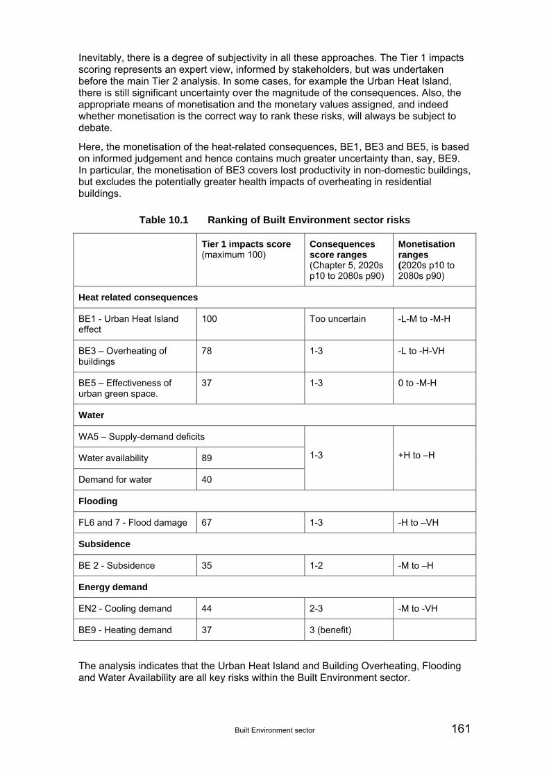
Built Environment sector 161
Inevitably, there is a degree of subjectivity in all these approaches. The Tier 1 impacts scoring represents an expert view, informed by stakeholders, but was undertaken before the main Tier 2 analysis. In some cases, for example the Urban Heat Island, there is still significant uncertainty over the magnitude of the consequences. Also, the appropriate means of monetisation and the monetary values assigned, and indeed whether monetisation is the correct way to rank these risks, will always be subject to debate.
Here, the monetisation of the heat-related consequences, BE1, BE3 and BE5, is based on informed judgement and hence contains much greater uncertainty than, say, BE9. In particular, the monetisation of BE3 covers lost productivity in non-domestic buildings, but excludes the potentially greater health impacts of overheating in residential buildings.
Table 10.1 Ranking of Built Environment sector risks
Tier 1 impacts score (maximum 100)
Consequences score ranges (Chapter 5, 2020s p10 to 2080s p90)
Monetisation ranges (2020s p10 to 2080s p90)
Heat related consequences
BE1 - Urban Heat Island effect
100 Too uncertain -L-M to -M-H
BE3 – Overheating of buildings
78 1-3 -L to -H-VH
BE5 – Effectiveness of urban green space.
37 1-3 0 to -M-H
Water
WA5 – Supply-demand deficits
Water availability 89
Demand for water 40
1-3 +H to –H
Flooding
FL6 and 7 - Flood damage 67 1-3 -H to –VH
Subsidence
BE 2 - Subsidence 35 1-2 -M to –H
Energy demand
EN2 - Cooling demand 44 2-3 -M to -VH
BE9 - Heating demand 37 3 (benefit)
The analysis indicates that the Urban Heat Island and Building Overheating, Flooding and Water Availability are all key risks within the Built Environment sector.

162 Built Environment sector
As temperatures rise, heat-related risks pose a threat both to human health and comfort and to productivity, yet there is a lack of policy drivers and an urgent need for further research in this area. The phenomenon of building overheating is closely inter-related with the Urban Heat Island and green infrastructure.
Recent research has indicated that, currently, the thermal performance of a building and its local microclimate, as determined by greening in the immediate vicinity, make a greater contribution to its overheating risk than its location within the Urban Heat Island. This highlights the need for an integrated approach to adaptation. Where possible, passive cooling measures should be implemented at building level to improve thermal comfort. This will avoid exacerbation of the Urban Heat Island by widespread adoption of air-conditioning.
In addition, green infrastructure on all scales is needed to provide local shading and cooling benefits. However, management and maintenance practices for urban green space may need to change, for example through planting of climate change resilient species and effective water management strategies in hot, dry periods, to prevent a loss of cooling capacity.
Lack of water availability and increased risk of flooding are also key risks within the Built Environment sector. However, adaptive capacity is higher than for heat-related issues. Climate change is already incorporated, albeit simplistically, within the Water Resources Periodic Review. The Flood and Water Management Act 2010 provides for more comprehensive management of flood risk for people, homes and businesses.
Subsidence is a major economic risk, which could increase with changing rainfall patterns. The risk would be expected to decrease as old buildings are replaced with more modern constructions, but the turnover of existing stock is still extremely low (typically 1% per annum), especially in the domestic sector.
Energy demand for winter heating is projected to fall. This provides an opportunity for innovation in design. Nonetheless there is a danger that the current focus on improving winter energy efficiency of new and existing buildings may reduce their capacity to withstand prolonged warm periods, which are projected to become more frequent in future.
Many of these impacts and consequences would have a disproportionate effect on socially vulnerable groups. For example, heat stress is most likely to affect the elderly, those in hospitals or care homes, the very young and those with underlying health problems. The Urban Heat Island effect has already contributed to excess deaths during recent heatwaves, particularly amongst the elderly, and this is projected to increase. Furthermore, socially disadvantaged members of society may not have the financial resources to adapt by themselves.
Overall, climate change presents an opportunity to seek to maximise the efficiency of both new and existing buildings, both domestic and non-domestic, and to promote the use of passive design principles rather than an over reliance on mechanical means of providing thermal comfort. However, given the low adaptive capacity of the Built Environment sector, in which the chief driver is capital cost, such adaptation may not happen on an autonomous basis. Given the low replacement rate of existing building stock, refurbishment and retrofit adaptation work is as important in coping with a future changing climate as standards for new-build projects.

Built Environment sector 163
11 References Other CCRA Sector Reports
Baglee, A., Haworth, A. and Anastasi, S. (2012) CCRA Risk Assessment for the Business, Industry and Services Sector. UK 2012 Climate Change Risk Assessment, Defra, London.
McColl, L., Angelini, T. and Betts, R. (2012) CCRA Risk Assessment for the Energy Sector. UK 2012 Climate Change Risk Assessment, Defra, London.
Moffat, A.J., Morison, J.I.L., Nicoll, B., and Bain, V. (2012) CCRA Risk Assessment for the Forestry Sector. UK 2012 Climate Change Risk Assessment, Defra, London.
Brown, I., Ridder, B., Alumbaugh, P., Barnett, C., Brooks, A., Duffy, L., Webbon, C., Nash, E., Townend, I., Black, H. and Hough, R. (2012) CCRA Risk Assessment for the Biodiversity and Ecosystem Services Sector. UK 2012 Climate Change Risk Assessment, Defra, London.
Hames, D. and Vardoulakis, S. (2012) CCRA Risk Assessment for the Health Sector. UK 2012 Climate Change Risk Assessment, Defra, London.
Knox, J.W., Hurford, A., Hargreaves, L. and Wall, E. (2012) CCRA Risk Assessment for the Agriculture Sector. UK 2012 Climate Change Risk Assessment, Defra, London.
Ramsbottom, D., Sayers, P. and Panzeri, M. (2012) CCRA Risk Assessment for the Floods and Coastal Erosion Sector. UK 2012 Climate Change Risk Assessment, Defra, London.
Rance, J., Wade, S.D., Hurford, A.P., Bottius, E. and Reynard, N.S. (2012) CCRA Risk Assessment for the Water Sector. UK 2012 Climate Change Risk Assessment, Defra, London.
Thornes, J., Rennie, M., Marsden, H. and Chapman, L. (2012) CCRA Risk Assessment for the Transport Sector. UK 2012 Climate Change Risk Assessment, Defra, London.
Pinnegar, J., Watt, T., and Kennedy, K. (2012) CCRA Risk Assessment for the Marine and Fisheries Sector. UK 2012 Climate Change Risk Assessment, Defra, London.
Other CCRA Reports
Ballard, D. (2009) Working paper on adaptive capacity. Working paper 1 for the UK’s Climate Change Risk Assessment 2012. Alexander Ballard Ltd for HR Wallingford Ltd.
CCRA (2011) Systematic mapping report. UK 2012 Climate Change Risk Assessment, Defra, London.
Defra (2010a) Method for undertaking the CCRA, UK 2012 Climate Change Risk Assessment, Defra, London.
Defra (2010b) Method for undertaking the CCRA Part II - Detailed Method for Stage 3: Assess Risk, UK 2012 Climate Change Risk Assessment, Defra, London.
CCRA (2012) CCRA Evidence Report. UK 2012 Climate Change Risk Assessment, Defra, London.
CCRA (2012a) Devolved Administration and English Area Report: Volume 1: A climate change risk assessment for Northern Ireland, UK 2012 Climate Change Risk
164 Built Environment sector
Assessment, Defra, London. Report by HR Wallingford Ltd, The Met Office, Alexander Ballard Ltd, Collingwood Environmental Planning, Entec Ltd UK, Paul Watkiss Associates, Metroeconomica.
Other References
Acclimatise Ltd (2010), http://www.acclimatise.uk.com/resources/reports.
AEA (2010) Greenhouse Gas Inventories for England, Scotland, Wales and Northern Ireland: 1990 – 2008. Available http://uk-air.defra.gov.uk/reports/cat07/1009070945_DA_GHGI_report_2008_maintext_Issue_1.pdf
AECOM (2010) Adapting English Schools Sites to reduce the predicted overheating impacts resulting from Climate Change, Department for Education, London.
Armstrong B., Chalabi Z., Fenn B., Hajat S., Kovats S., Milojevic A. and Wilkinson P. (2010) Association of mortality with high temperatures in a temperate climate: England and Wales. Journal of Epidemiology Community Health.
ASC (2010) How well prepared is the UK for climate change? First report of the Adaptation Sub-Committee, 16 September 2010.
ASC (2011) Adapting to climate change in the UK: Measuring progress, Adaptation Sub-Committee Progress Report 2011.
Austin P, Rydin Y, Maslin M (2008) Climate Change – The Risks for Property in the UK, UCL Environment Institute for Hermes Real Estate.
Baxter P (2005) The East Coast Great Flood, 31 January - 1 February 1953: A Summary of the Human Disaster. Philosophical Transactions of the Royal Society. Series A.
BB 90 (1999) Department for Education and Employment, Building Bulletin 90: Lighting Design for Schools, 1999.
BB 93 (2004) Department for Education and Skills, Building Bulletin 93: Acoustic Design of Schools, 2004.
BB 101 (2006) Department for Education, Building Bulletin 101: Ventilation of School Buildings, 2006.
Bohnenstengel S et al. (2010) International Association for Urban Climate, Issue No. 36, 2010.
Bohnenstengel SI, Evans S, Clark PA and Belcher SE (2011) Simulations of the London urban heat island, Q.J.R. Meteorol. Soc.
Bowler, D., Buyung-Ali, L., Knight, T. & Pullin, A.S (2010) How effective is ‘greening’ of urban areas in reducing human exposure to ground level ozone concentrations, UV exposure and the ‘urban heat island effect’? Environmental Evidence: www.environmentalevidence.org/SR41.html
British Standards Institution (1992) Code of practice for assessing exposure of walls to wind-driven rain, British Standard BS 8104:1992, London, BSI 1992.
Buildoffsite (2009) Offsite Production in the UK Construction Industry – prepared by HSE and published by Buildoffsite, June 2009 www.buildoffsite.com
CABE (2009) Making the invisible visible: the real value of park assets, CABE, February 2009.

Built Environment sector 165
Capon R (2010) Built Environment Sector Early Report, February 2010.
Cassar M (2002) Climate Change and the Historic Environment. Report by UCL for English Heritage. Available at: http://www.climatechangeandyourhome.org.uk/live/content_pdfs/Climate%20Change%20and%20the%20Historic%20Environment%202.pdf
Cazenave, A and Llovel W (2010) Contemporary Sea Level Rise. Annual Review of Marine Science, 2, 145-173.
CEBR (2003) Press release.
Chatterton J, Morris J, Viavattene C, Penning-Rowsell E and Tapsell S (2009) The costs of the summer 2007 floods in England. Final Project Report: SC070039/R1. Environment Agency.
CIBSE (2005) Climate change and the indoor environment: impacts and adaptation, CIBSE TM36: 2005.
CIBSE (2006) Guide A: Environmental Design.
City of London (2007) Rising to the Challenge-The City of London Corporation’s Climate Adaptation, January 2007.
Cole, G.A. and Marsh, T.J. (2005) Major droughts in England and Wales from 1800 and evidence of impact, Science Report SC030298/SR, Environment Agency.
Coley D A, Greeves R (2004) Report R102 for DfES, the effect of low ventilation rates on the cognitive function of a primary school class, Exeter University.
Comiso, JC, Parkinson, CL, Gernsten L, and Stock, L (2008) Accelerated decline in the Arctic sea ice cover. Geophysical Research Letters, 35, L01703.
Communities and Local Government (2009) Household Projections to 2031, England. Housing Statistical Release. 11/03/09. Available at: http://www.communities.gov.uk/documents/statistics/pdf/1172133.pdf.
COPSE project, Co-Incident Probabilistic Climate Change Weather Data for a Sustainable Environment http://www.copse.manchester.ac.uk/
Council of Mortgage Lenders (2010) http://www.cml.org.uk/cml/media/press/2745 (accessed 10th Dec 2010).
Crump D, Dengel A and Swainson M (2009) Indoor air quality in highly energy efficient homes – a review, NHBC Foundation report NF18, IHS BRE Press.
Davis I, Harvey V (2008) Zero Carbon: what does it mean to homeowners and housebuilders? NHBC Foundation report, NF9.
Day A R, Jones P G, Maidment G G (2009) Forecasting future cooling demand in London. Energy and Buildings 41 (2009) 942–948.
DCLG (2011) Departmental Adaptation Plan - Update May 2011.
Defra (2000) Guidelines for Environmental Risk Assessment and Management. At: http://www.defra.gov.uk/environment/quality/risk/eramguide/index.htm
Defra (2008) Future Water: The Government’s water strategy for England. HMSO, Norwich, UK. 98pp.
Defra (2009) UK Climate Projections. At: http://ukclimateprojections.defra.gov.uk/

166 Built Environment sector
Defra (2011) Water for Life (The Water White Paper), December 2011. http://www.official-documents.gov.uk/document/cm82/8230/8230.pdf (Accessed 08/12/11)
Defra Flooding and Coastal Change http://ww2.defra.gov.uk/environment/flooding/ accessed 26 July 2011.
DECC (2009) The Road to Copenhagen. The UK Government’s case for an ambitious international agreement on climate change. The Department for Energy and Climate Change, London.
DECC (2010a) Energy Consumption in the UK. Published by the Department for Energy and Climate Change. Available at: http://www.decc.gov.uk/assets/decc/statistics/publications/ecuk/file11250.pdf
DECC (2010b) Valuation of energy use and greenhouse gas emissions for appraisal and evaluation, June 2010. Department of Climate Change/ HM Treasury. Available at: http://www.decc.gov.uk/assets/decc/statistics/analysis_group/122-valuationenergyuseggemissions.pdf
DECC (2010c) 2050 Pathways Analysis Report. Available at http://www.decc.gov.uk/en/content/cms/tackling/2050/2050.aspx
Department of Health (1999) Economic Appraisal of the Health Effects of Air Pollution. Ad-Hoc Group on the Economic Appraisal of the Health Effects of Air Pollution. London. The Stationery Office.
Department of Health (2010) Heatwave Plan for England, Protecting Health and Reducing Harm from Extreme Heat and Heatwaves.
Department of Health (2011) No health without mental health: a cross-government mental health outcomes strategy for people of all ages, Department of Health, February 2011.
De2RHECC (2010) Design and Delivery of Robust Hospital Environments in a Changing Climate (continues to 2012) www.robusthospitals.org.uk
Dlugolecki A (2004) A changing climate for insurance. A summary report for Chief Executives and Policymakers. ABI, London.
Donaldson G., Kovats R.S., Keatinge W.R. and McMichael A.J. (2002) Heat and Cold Related Mortality and Morbidity and Climate Change. In: Health Effects of Climate Change in the UK. Department of Health. London. pp 70-80.
Dousset B, Gourmelon F, Laaidi K, Zeghnoun A, Giraudet E, Bretin P, Mauri E, Vandentorren S (2011) Satellite monitoring of summer heat waves in the Paris metropolitan area. International Journal of Climatology; Feb2011, Vol. 31 Issue 2, p313-323.
Driscoll R M C and Crilly M S (2000) Subsidence damage to domestic buildings: lessons learned and questions remaining. FBE Report 1. CRC Ltd.
Driscoll R and Skinner H (2007) Subsidence damage to domestic buildings: a guide to good technical practice. FB13, Garston: BRE Trust.
English Heritage (2008) Climate Change and the Historic Environment. Available at http://www.climatechangeandyourhome.org.uk/live/content_pdfs/29.pdf
Environment Agency (2006) Addressing Environmental Inequalities: Flood Risk, Lancaster University on behalf of the Environment Agency, Project SC020061/SR1.
Built Environment sector 167
Environment Agency (2008) Water resources in England and Wales – current state and future pressures. Environment Agency, Bristol, UK. 23pp.
Forest Research (2010) Benefits of green infrastructure. Report to Defra and DCLG. Forest Research, Farnham.
Friedlingstein, P, Houghten, RA, Marland, G, Hacklar, J, Boden, TA, Conway, TJ, Canadell, JG, Raupach, MR, Ciais, P and Le Quéré, C. (2010) Update on CO2 emissions. Nature Geosciences, 3, 811-812.
Gazzard R (2010) Development of wildfire statistics and risk impacts in the United Kingdom, Fire and Rescue Statistics User Group (FRSUG). http://www.frsug.org/reports
Gething B (2010) Design for Future Climate: Opportunities for Adaptation in the Built Environment, Technology Strategy Board.
Gill S, Handley J, Ennos R and Pauleit S (2007) Adapting cities for climate change: the role of green infrastructure, Built Environment, Vol 33, No 1, pages 115 – 133.
Graves H M and Phillipson M C (2000) Potential implications of climate change in the built environment. FBE Report 2. CRC Ltd.
Greater London Authority (2010a) Right trees for a changing climate. Greater London Authority. http://www.right-trees.org.uk/default.aspx
Greater London Authority (2010b) The draft climate change adaptation strategy for London. Available from http://legacy.london.gov.uk/mayor/priorities/docs/Climate_change_adaptation_080210.pdf
Hajat S., Kovats R.S. and Lachowycz K. (2007) Heat-Related and Cold-Related Deaths in England and Wales: Who is at Risk? Occupational and Environmental Medicine. Volume 64. pp 93-100.
Hall, J.W., Dawson, R.J., Walsh, C.L., Barker, T., Barr, S.L., Batty, M., Bristow, A.L., Burton, A., Carney, S., Dagoumas, A., Evans, S., Ford, A.C., Glenis, V., Goodess, C.G., Harpham, C, Harwatt, H., Kilsby, C., Köhler, J., Jones, P., Manning, L., McCarthy, M., Sanderson, M., Tight, M.R., Timms, P.M. and Zanni, A.M. (2009) Engineering Cities: How can cities grow whilst reducing emissions and vulnerability? Newcastle University, October, 2009. (ISBN 978-0-7017-0225-0).
HCA (2009) Affordable Housing Survey: A Review of the quality of affordable housing in England.
HM Government (2009) The UK Low Carbon Transition Plan: National strategy for climate and energy. Presented to Parliament pursuant to Sections 12 and 14 of the Climate Change Act 2008. Published by the Stationary Office.
H.M. Treasury (2003) The Treasury Green Book – Appraisal and Evaluation in Central Government. At: http://www.hm-treasury.gov.uk/data_greenbook_index.htm
HMT (2007) The Green Book. Appraisal and Evaluation in Central Government Treasury Guidance. Her Majesty’s Treasury. London: TSO.
HMT (2008) Intergenerational wealth transfers and social discounting: Supplementary Green Book guidance July 2008, http://www.hm-treasury.gov.uk/d/4(5).pdf.
HMT (2009) Accounting for the Effects of Climate Change. June 2009. Supplementary Green Book Guidance, Available at http://www.hm-treasury.gov.uk/data_greenbook_supguidance.htm#Adaptation_to_Climate_Change.
168 Built Environment sector
HTM 03-01A (2007) Department of Health Estates and Facilities, Health Technical Memorandum 03-01: Specialised Ventilation for Healthcare Premises - Part A: Design and Validation Heating and Ventilation Systems, 2007.
HTM 55 (1998) Department of Health Estates and Facilities, Health Technical Memorandum 55 Windows (first published 1989, second edition 1998).
Hunt A and Taylor T (2006) Buildings. Chapter 7 In. Metroeconomica (2006). Climate Change Impacts and Adaptation: Cross-Regional Research Programme Project E. Published by Defra, London.
IGCB (2007) An Economic Analysis to Inform the Air Quality Strategy, Updated Third Report of the Interdepartmental Group on Costs and Benefits. Published by the IGCB, London.
IGCB (2010) The appraisal of climate change impacts of air pollution. Published by the Interdepartmental Group on Costs and Benefits (IGCB), London.
IPCC (2007) Climate Change 2007: The physical science basis. Contribution of working group I to the fourth assessment report of the Intergovernmental Panel on Climate Change [Solomon, S., Qin, D., Manning, M., Chen, Z., Marquis, M., Averyt, K. B., Tignor, M. and Miller, H. L. (eds.)]. Cambridge University Press, Cambridge, United Kingdom and New York, NY, USA, 996 pp.
ISCCC (2009) International Scientific Congress Climate Change: Global Risks, Challenges & Decisions – Synthesis Report. ISCCC, Copenhagen.
James S, (2011) Review of Education Capital, April 2011, available at http://media.education.gov.uk/assets/files/pdf/c/review of education capital.pdf
Jenkins, GJ, Perry, MC, and Prior, MJO (2009) The Climate of the United Kingdom and Recent Trends. Met Office Hadley Centre, UK.
Johnson H, Kovats S, McGregor G, Stedman J, Gibbs M and Walton H (2005) The impact of the 2003 heat wave on daily mortality in England and Wales and the use of rapid weekly mortality estimates,Euro Surveillance: European Communicable Disease Bulletin 2005, 10(7):168-71.
Kjellstrom T, Kovats R S, Lloyd S J, Holt T and Tol R S (2009) The direct impact of climate change on regional labour productivity. Arch Environ Occup Health. 2009 Winter; 64(4):217-27.
Knight S (2010) Mapping Manchester’s urban heat island, Weather – July 2010, Vol 65, No.7.
Kolokotroni M, Davies M, Croxford B, Bhuiyan S and Mavrogianni A (2010) A validated methodology for the prediction of heating and cooling energy demand for buildings within the Urban Heat Island: Case-study of London, Solar Energy 84 (2010) 2246–22.
Kovats S., Armstrong B. and Hunt A. (2006) Climate Change Impacts and Adaptation: Cross Regional Research Programme - Quantify the Costs of Impacts and Adaptation - GA01075. In Metroeconomica (2006) Defra, London.
Kronos (2007) Sunny Skies and High Temperatures Have Employees Suffering From Seasonal Absence Syndrome, www.kronos.com
Le Quéré, C., Raupach, MR, Canadell, JG, and Marland GM (2009) Nature Geosciences, 2, 831-836.
Lindner, M., Maroschek, M., Netherer, S., Kremer, A., Barbati, A., Garcia-Gonzalo, J., Seidl, R., Delzon, S., Corona, P., Kolstrom, M., Lexer, M. J. and Marchetti, M. (2010)

Built Environment sector 169
Climate change impacts, adaptive capacity and vulnerability of European forest ecosystems. Forest Ecology and Management, 259, 698 – 709.
London Assembly (2007) Chainsaw massacre - A review of London’s street trees.
London Climate Change Partnership (2009) Commercial Building Stock and Climate Change Adaptation: Costs, Value and Legal Implications, London Climate Change Partnership – Finance Group.
London Climate Change Partnership (2009a) Adapting to climate change: Creating natural resilience Summary Report, GLA available at www.london.gov.uk/lccp
LUCID project (2007-2010) The Development of a Local Urban Climate Model and its Application to the Intelligent Design of Cities http://www.lucid-project.org.uk/
Mavrogianni A et al. (2009) Space heating demand and heatwave vulnerability: London domestic stock, Building Research & Information 37 (5 – 6), 583 – 597.
Mavrogianni A, Davies M, Wilkinson P and Pathan A (2010) London housing and climate change: impact on comfort and health – preliminary results of a summer overheating study. Open House 53(2), 49-59.
Mayor of London (2006) London’s urban heat island: A summary for decision makers. Greater London Authority: London.
McCarthy M P et al. (2010) Climate change in cities due to global warming and urban effects. Geophys. Res. Lett., 37, L09705, doi:10.1029/2010GL042845.
McCarthy M.P., Harpham C, Goodess C, and Jones P (2011) Simulating climate change in UK cities using a regional climate model, HadRM3. submitted to Int. J. Climatol.
McMorrow J., Aylen, J., Albertson, K., Cavan, G., Lindley, S., Handley, J., and Karooni, R. (2005) Change and the Visitor Economy Technical Report 3: Moorland Wildfires in the Peak District, University of Manchester.
Metroeconomica (2006) Climate Change Impacts and Adaptation: Cross-Regional Research Programme Project E.
Milojevic A, Wilkinson P, Armstrong Ben, Davis M, Mavrogianni Anna, Bohnenstengel S, Belcher S (2011) Impact of London's Urban Heat Island on Heat-related Mortality, Epidemiology. 22(1):S182-S183, January 2011.
Mott MacDonald (1998) The Review of Costs To Balance Supply and Demand Project 2. Report Ref: 48550/WSD/02/B. Final Report. August 1998.
National Trust, stakeholder response in Capon (2010).
Nicol, J.F., Hacker J., Spires B. and Davies H. (2009) Suggestion for new approach to overheating diagnostics, Building Research & Information, 37:4, 348-357.
NIOSH (1986) Criteria for a Recommended Standard: Occupational Exposure to Hot Environments (Revised Criteria 1986), The National Institute for Occupational Safety and Health (NIOSH), USA, Report No: Publication No. 86-113, 1-151.
Ofwat (2010) Delivering sustainable water – Ofwat’s strategy. Available at: http://www.ofwat.gov.uk/aboutofwat/reports/forwardprogrammes/rpt_fwd_20100303ofwatstrategy.pdf
ONS (2007) The ONS Productivity Handbook A Statistical Overview and Guide. Office for National Statistics. Available at http://www.ons.gov.uk/about-statistics/user-guidance/productivity-handbook/index.html

170 Built Environment sector
ONS (2010) Labour Productivity. Available at http://www.statistics.gov.uk/StatBase/Product.asp?vlnk=7476
Ostro B., Rauch S., Green R., Malig B. and Basu R. (2010) The Effects of Temperature and Use of Air Conditioning on Hospitalizations, American Journal of Epidemiology, Volume 172, Issue 9, pp 1053-1061.
PARNASSUS Protecting Cultural Heritage From Flood And Driven Rain http://www.bath.ac.uk/parnassus/
Parsons, K. (2009) Maintaining health, comfort and productivity in heat waves, Global Health Action, Vol. 2, pp. 2057.
Pitt (2008) Learning Lessons from the 2007 Floods, Independent Review chaired by Sir Michael Pitt, April 2008.
Roaf, Crichton and Nicol (2009) Adapting Buildings And Cities For Climate Change: a 21st century survival guide, Oxford: Elsevier.
Ruckerl R, Green S, Ljungman P, Aalto P, Antoniades C, Bellander T, Berglind N, Chrysohoou C, Forastiere F, Jacquemin B, Von Klot S, Koenig W, Kuchenhoff H, Lanki T, Pekkanen J, Perucci C A, Schneider A, Sunyer J and Peters A (2007) Air Pollution and inflammation (interleukin-6, C-reactive protein, fibrinogen) in myocardial infarction survivors. Environ Health Perspect, 115(7). pp 1072-1080.
Sabbioni C, Cassar M, Brimblecombe P and Lefevre RA (2008) Vulnerability of Cultural Heritage to Climate Change, Report for E. FERNANDEZ-GALIANO, Council of Europe European and Mediterranean Major Hazards Agreement (EUR-OPA), 6 November 2008.
Sanders, C.H. and Phillipson, M.C. (2003) UK adaptation strategy and technical measures: the impacts of climate change on buildings, Building Research and Information 31(3-4): 210-221.
Sanders CH, Phillipson MC and Hunter CA (2004) Future Challenges for Air-Quality and Health in Housing, New Horizons Project DO3 Final Report and Technical Report, Prepared for Office of the Deputy Prime Minister, New Horizons Programme.
SCIENCE AND HERITAGE PROGRAMME funded by the Arts & Humanities Research Council and Engineering and Physical Sciences Research Council http://www.heritagescience.ac.uk/
SCORCHIO project (2007-2010) Sustainable Cities: Options for Responding to climate CHange Impacts and Outcomes http://www.sed.manchester.ac.uk/research/cure/research/scorchio/
The Scottish Government (2009) Scotland’s Climate Change Adaptation Framework– The Built Environment http://www.scotland.gov.uk/Publications/2009/12/08130803/1
The Scottish Government (2010) Planning and Climate Change: Key Agency & Scottish Government Resources and Guidance http://www.scotland.gov.uk/Topics/Built-Environment/planning/modernising/cc/Climatechange
Shaw R, Colley M and Connell R (2007) Climate change adaptation by design: a guide for sustainable communities. TCPA, London.
SHINE Network (2010) CIRIA, Research Project for the National Institute for Healthcare Research, Making Existing Healthcare Buildings Sustainable 2010.
Smith C, Webb A, Levermore GJ, Lindley SJ and Beswick K (2011) Fine-scale spatial temperature patterns across a UK conurbation, Climatic Change.

Built Environment sector 171
South East of England Regional Wildfire Group and Home Counties Operational Wildfire Group (2010) Building our resilience to wildfires: preparation and prevention for 2012, April 2010.
Stirling C (2002) Thermal Insulation: Avoiding Risks, BRE.
Stott PA, Stone DA and Allen MR (2004) Human contribution to the European heatwave of 2003. Nature, 432, 610-614. Corrigem. Nature, 436, 1200.
TCPA (2010) Planning and Climate Change Guide: guidance and model policies for local authorities - TCPA, in conjunction with the RTPI (Nov 2010).
Thomas M et al. (1998) Brain and behaviour changes during sleep deprivation, Proc. Human Factors and Ergonomics Society 2.
Tomlinson CJ, Chapman L, Thornes JE and Baker CJ (2010) Derivation of Birmingham’s summer surface urban heat island from MODIS satellite images, International Journal of Climatology (published online 3 Dec 2010).
Trotman P, Sanders C and Harrison H (2004) Understanding Dampness, BRE Bookshop.
Twigger-Ross C and Orr P (2011) Social vulnerability to climate impacts. UK 2012 Climate Change Risk Assessment, Defra, London.
UKCIP (2003) Climate adaptation: Risk, uncertainty and decision making. Willows, R. and Connell, R., UK Climate Impacts Programme, Oxford, UK.
UK Green Building Council (2007) Report on carbon reductions in new non-domestic buildings, Report from UK Green Building Council, December 2007, Department for Communities and Local Government
Unwin D J (1980) The Synoptic Climatology of Birmingham’s Urban Heat Island, 1965 – 74, Weather 35: 43–50.
Vassallo M., Gera K.N., and Allen S (1995) Factors Associated with High Risk of Marginal Hyperthermia in Elderly Patients Living in an Institution. Postgraduate Medical Journal. Volume 71. Number 834. pp 213-216.
Walker, M. and Burgess, D. (2007) Preliminary Cost Effectiveness Analysis (pCEA) of Water Resources Measures to meet WFD Environmental Objectives.
The Walker Review (2009) The Independent Review of Charging for Household Water and Sewerage Services, Final Report, Anna Walker, published by Defra, December 2009.
Watkiss P., Hunt A. and Horrocks L. (2009) Literature Review: Scoping Study for a National Climate Change Risk Assessment and Cost-Benefit Analysis. Metroeconomica, AEA group, and Paul Watkiss Associates.
Wilkinson P., Pattenden S., Armstrong B., Fletcher A., Kovats R.S., Mangtanu P. and McMuchael A.J. (2004) Vulnerability to Winter Mortality in Elderly People in Britain: Population Based Study. British Medical Journal. Volume 329(7467). pp 647-651.
Wolf J., Adger W.N., Lorenzoni I., Abrahamson V. and Raine R. (2010) Social Capital, Individual Responses to Heat Waves and Climate Change Adaptation: An Empirical Study of Two UK cities. Global Environmental Change. Volume 20. pp 44-52.

172 Built Environment sector
Data sets
Armstrong B, Chalabi Z, Fenn B, Hajat S, Kovats S, Milojevic A and Wilkinson P (2010) Association of mortality with high temperatures in a temperate climate: England and Wales. Journal of Epidemiology Community Health.
UKCP09 web site: http://ukclimateprojections-ui.defra.gov.uk
Met Office Hadley centre observation datasets web site: http://hadobs.metoffice.com/index.html
ABI Table 8: Domestic Subsidence – Gross Incurred Claims.
Building statistics:
DCLG - England
About housing
http://www.communities.gov.uk/housing/about/
Housing statistics
http://www.communities.gov.uk/housing/housingresearch/housingstatistics/housingstatisticsby/
http://www.communities.gov.uk/housing/housingresearch/housingsurveys/englishhousingsurvey/ehstables/
http://www.communities.gov.uk/documents/statistics/xls/1750447.xls
Wales
Housing statistics
http://www.statswales.wales.gov.uk/TableViewer/tableView.aspx?ReportId=18911
Projections
http://wales.gov.uk/topics/statistics/theme/housing/estimate/hsehold-proj/?lang=en
http://wales.gov.uk/topics/statistics/theme/housing/stock/;jsessionid=w3P8TJBTLZDvS2fpkgRMN3xMgRn6yQ9hp3pyj3f3QgmmWGvz9pBh!-1092479367?lang=en
Scotland
Projections
http://www.scotland.gov.uk/Topics/Statistics/Browse/Housing-Regeneration/PubHouseholdProjections
Statistics
http://www.scotland.gov.uk/Topics/Statistics/Browse/Housing-Regeneration/HSfS/KeyInfoTables
Northern Ireland
http://www.nisranew.nisra.gov.uk/census/censusstatistics/1991/1991housing.html (updated statistics required)

Built Environment sector 173
Appendices

174 Built Environment sector

Built Environment sector 175
Appendix 1 The Tier 1 List
This Appendix contains the Tier 1 list for the Built Environment sector including impacts and consequences.
The impacts to the built environment can generally be classified as:
Damage to buildings caused by extreme storm events (including extreme rainfall and wind).
Damage to buildings caused by increased temperatures and dryer summers. This includes damage to foundations caused by changes in soil stability, damage to underground services and heat effects on building fabric.
Increase in temperature in buildings and the surrounding areas, including extreme heat waves. Vulnerable people will be particularly affected.
Climate change also presents opportunities for the built environment particularly in the reduction in winter heating demands and problems caused by ice and snow.
The following points should be considered when using the data:
Where the same or similar impacts have been identified, attempts have been made to remove duplicates. However, where there are subtle differences between impacts, similar impacts have been retained as separate impacts in the spreadsheet.
There are many potentially adverse impacts but also a number of opportunities have been identified. A preliminary assessment has been made of threats (adverse impacts) and opportunities in the tables using the following colour code:
T= threat (red), O = opportunity (green); N = neutral impact (amber).
However it is recognised that there may be both positive and negative aspects of the same impact.

176 Built Environment sector
Tier 1 list of climate change impacts
Climate effects Impacts T/O/N Consequences Comments
Main climate driver: Increase in storms including extreme precipitation, extreme wind and surge tides
1. Storm surges / sea-level rise
Increase in flooding of coastal areas, including coastal archaeology and landscapes, green space R
Flood damage: Increase in damage to land and property, including historic sites and buildings. Implications for land use in future, increase demand for flood defences for developments; influence location of key infrastructure
Significant impact. Clustered with impacts 2, 3, 4, 10, 21, 22 and 23. Assessed in Floods Sector (Metrics FL6 and FL7)
2. Increase in frequency of intense precipitation events; increase in winter rainfall
Increase in fluvial flooding of urban areas and buildings
R
Flood damage: Increase in damage to land and property; disruption of services making reinstatement of the building more difficult; increase in relative humidity levels leading to pests and mould. High cost of claims. Implications for land use in the future. Premises inaccessible
Significant impact. Clustered with impacts 1, 3, 4, 10, 21, 22 and 23. Assessed in Floods Sector (Metrics FL6, FL7 and FL13)
3. Increase in frequency of intense precipitation events
Increase in pluvial flooding in urban areas
R
Flood damage: Overwhelming of sewers causing them to back up, increase in flooding by water contaminated by raw sewage; damage to land and property; pollution of rivers
Significant impact. Clustered with impacts 1, 2, 4, 10, 21, 22 and 23. Assessed in Floods Sector (Metrics FL6 and FL7)
4. Increase in frequency of intense precipitation events
Increase in flash flooding
R
Flood damage: Increase in flooding ; damage to emergency infrastructure; damage to property
Significant impact. Clustered with impacts 1, 2, 3, 10, 21, 22 and 23. Assessed in Floods Sector (Metrics FL6 and FL7)
5. # Increase in intense precipitation events
Soil erosion
R
Competition for land and increasing tensions between land use objectives
Marginal score. Clustered with impact 6.
6. Increase in winter rainfall; increase in frequency of extreme rainfall events
Increase in landslips
R
Increased damage to buildings; implications for what particular land can be used for in the future
Marginal score. Clustered with impact 5.
7. Increase in wind-driven rain - increase in winter rainfall; increase in frequency of intense rainfall events
Increase in rainwater penetration of buildings
R
Water damage: Increase in damage to buildings including historical sites and buildings; increase in maintenance required; higher humidity leading to increase in pests and mould
Marginal score. Discussed in Section 3.4. Clustered with impact 8.
8. Increase in frequency of extreme rainfall events
Overwhelming of roofs and rainwater goods, particularly in historical buildings
R
Water damage: Increased penetration of driven rainwater (pluvial) into buildings through roofs and flashings and around windows
Marginal score. Discussed in Section 3.4. Clustered with impact 7.
9. Increase in frequency of windstorms
Structural damage to buildings
R
Storm damage: Increase in building damage. Loss of life in extreme cases
Low score. Not taken forward. Clustered with impacts 11 and 12.
10. Increase in wind-driven rain
Increase in surface water discharge from buildings
r
Flood damage: Increase in flooding elsewhere
Significant impact. Clustered with impacts 1, 2, 3, 4, 21, 22 and 23. Assessed in Floods Sector (Metrics FL6 and FL7)
11. Increase in frequency of windstorms
Tree damage/loss
r
Storm damage: Increase in severe damage to buildings; loss of life
Low score. Not taken forward. Clustered with impacts 9 and 12.

Built Environment sector 177
Climate effects Impacts T/O/N Consequences Comments
12. Change in storminess
Storm damage at construction sites
r
# Delays to construction Low score. Not taken forward. Clustered with impacts 9 and 11
Main climate driver: Changes in annual or seasonal precipitation
13. Drier summers (decrease in summer rainfall)
Impacts on water infrastructure, water shortage a
Adaptation of water infrastructure will have implications for where future developments can be located
Significant impact. Clustered with impact 14. Assessed in Water Sector (Metrics WA5 and WA6)
14. Decrease in summer rainfall
Decrease in water availability
r
Water availability: Decrease in water available for households; increase in tree management issues
Significant impact. Clustered with impact 13. Assessed in Water Sector (Metrics WA5 and WA6)
15. Decrease in summer rainfall
Drought impacts on infrastructure
r
Damage caused by drying: Increased damage caused by drying soils and loss of vegetation
Significant impact. Clustered with impact 40. Assessed in analysis (Metric BE2)
16. Drier summers (decrease in summer rainfall)
Shortage of water affecting construction r
# Delays to construction. Greater need to design for water efficiency
Low score. Not taken forward.
17. Drier summers (decrease in summer rainfall)
Reduced condensation and deterioration g
Marginal score. Discussed in Section 3.4. Clustered with impact 44.
18. Drier summers (decrease in summer rainfall)
Dry conditions in gardens help promote 'urban creep'
r Change in condition of spaces
Low score. Not taken forward
19. Decrease in summer rainfall; increase in average summer temperature - hot, dry conditions
Increase in tree roots attacking sewerage systems
r
Damage caused by drying: Increase in damage and failure of sewerage systems
Low score. Not taken forward. Clustered with impact 42
20. Wetter winters (increase in winter rainfall)
Change in condition of urban green spaces
a
Significant impact. Clustered with impact 46. Assessed in analysis (Metric BE5)
21. Increase in rainfall Flooding during construction and difficulties around unprotected on-site storage of materials
r # Damage and delays to construction. Construction companies will have to take account of the impact of these factors on the way they work
Significant impact. Clustered with impacts 1, 2, 3, 4, 10, 22 and 23. Assessed in Floods Sector (Metrics FL6 and FL7)
Main climate driver: Sea-level rise
22. Sea-level rise City inundation
r
Flood impacts: Increased disruption to urban economic function
Significant impact. Clustered with impacts 1, 2, 3, 4, 10, 21, and 23. Assessed in Floods Sector (Metrics FL6 and FL7)
23. # Sea-level rise; increase in winter rainfall
Flooding of development land
r
Increased tensions between land use objectives; land may become unsuitable for some purposes and more suitable for other uses. Development diverted from floodplain affecting green and brownfield sites
Significant impact. Clustered with impacts 2, 3, 4, 10, 21 and 22. Assessed in Floods Sector (Metrics FL6 and FL7)
Main climate driver: Changes in annual, seasonal or extreme temperature
24. Increase in average summer temperature; heat waves
Increase in overheating of buildings
r
Increase in heat: Increased impacts on health; serious impacts on vulnerable people; increase in maladaptation e.g. installation of air conditioning systems; buildings inadequate. Affects productivity
Significant impact. Assessed in analysis (Metric BE3)
25. Increase in average summer temperature
Increase in external overheating in high density areas
r
Increase in heat: Increased impacts on health and well-being; serious impacts on vulnerable people
Significant impact. Clustered with impact 39. Assessed in analysis (Metric BE1)
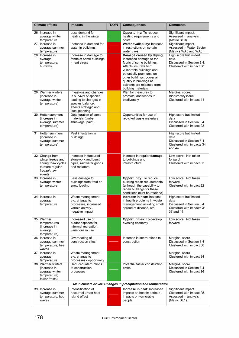
178 Built Environment sector
Climate effects Impacts T/O/N Consequences Comments
26. Increase in average winter temperature
Less demand for heating in the winter g
Opportunity: To reduce heating requirements and costs
Significant impact. Assessed in analysis (Metric BE9)
27. Increase in average summer temperature
Increase in demand for water in buildings r
Water availability: Increase in restrictions on certain water uses
Significant impact. Assessed in Water Sector (Metrics WA5 and WA6)
28. Increase in average temperature; humidity
Increase in damage to fabric of some buildings - heat stress
r
Damage caused by drying: Increased damage to the fabric of some buildings. Affects insurability of vulnerable buildings and potentially premiums on other buildings. Lower air quality in buildings as solvents are released from building materials
High score but limited data. Discussed in Section 3.4. Clustered with impact 30.
29. Warmer winters (increase in average winter temperature)
Invasions and changes in survival of species leading to changes in species balance, affects strategic and local planning
a
Plan for measures to promote landscapes to biodiversity
Marginal score. Biodiversity issue. Clustered with impact 41
30. Hotter summers (increase in average summer temperature)
Deterioration of some materials (timber shrinkage, paint) a
Opportunities for use of recycled waste materials
High score but limited data Discussed in Section 3.4 Clustered with impact 28
31. Hotter summers (increase in average summer temperature)
Pest infestation in buildings
r
High score but limited data Discussed in Section 3.4 Clustered with impacts 34 and 44
32. Change from winter freeze and spring thaw cycles to more regular freeze/thaw events
Increase in fractured stonework and burst pipes, rainwater goods and radiators
r
Increase in regular damage to buildings and infrastructure.
Low score. Not taken forward. Clustered with impact 33.
33. Increase in average winter temperature
Less damage to buildings from frost or snow loading g
Opportunity: To reduce building repair requirements (although the capability to repair buildings for these conditions must be retained)
Low score. Not taken forward Clustered with impact 32
34. Increase in average temperature
Waste management e.g. change to processes, increased vermin activity - negative impact
r
Increase in heat: Increase in health problems in waste management including smell, spread of disease, etc.
High score but limited data Discussed in Section 3.4 Clustered with impacts 31, 37 and 44
35. Warmer temperatures (increase in average temperature)
Increased use of outdoor spaces for informal recreation; variations in use
g
Opportunities: To develop evening economy
Low score. Not taken forward
36. Increase in average summer temperature; heat waves
Overheating of construction sites
r
Increase in interruptions to construction
Marginal score Discussed in Section 3.4 Clustered with impact 38
37. Increase in average temperature
Waste management e.g. change to processes - opportunity
g Marginal score
Clustered with impact 34
38. Warmer winters (increase in average winter temperature; fewer frosts)
Reduced interruptions to construction processes g
Potential faster construction times
Marginal score Discussed in Section 3.4 Clustered with impact 36
Main climate driver: Changes in precipitation and temperature
39. Increase in average summer temperature; heat waves
Intensification of nocturnal urban heat island effect r
Increase in heat: Increased impacts on health; serious impacts on vulnerable people
Significant impact. Clustered with impact 25. Assessed in analysis (Metric BE1)

Built Environment sector 179
Climate effects Impacts T/O/N Consequences Comments
40. Changes in rainfall and temperature - evaporation rates (# soil moisture)
Increase in ground movement (heave) and subsidence of clay soils
r
Damage caused by drying: Increase in movement of some building foundations; increase in pipe breakages affecting water availability and supply. Impacts on roads, bridges, embankments and tunnels
Significant impact. Clustered with impact 15. Assessed in analysis (Metric BE2)
41. Reduced soil moisture
Change in species balance with changed soil conditions
a Implications for strategic and local planning
Marginal score Biodiversity issue. Clustered with impact 29
42. Changes in rainfall and temperature - evapotranspiration rates
Increase in shrinkage of tree roots due to drying and swelling due to rehydration
r
Damage caused by drying: Increase in movement of some building foundations; indirect threat to green infrastructure as insurers demand that individual trees be taken out; increase in pipe breakages.
Low score. Not taken forward. Clustered with impact 19
43. Increase in average summer temperature; decrease in summer rainfall (hot, dry periods)
Increase in fire starting or spreading in buildings / increased fire fighting
r
Damage caused by drying: Increase in potential fire damage, particularly to historic thatched properties
Low score. Not taken forward
44. Milder, wetter winters
Increase in damp, mould and insect pests in buildings
r
Water damage: Increase in building damage and repair requirements.
High score but limited data Discussed in Section 3.4 Clustered with impacts 17, 31 and 34
45. Warmer, wetter conditions
Impact on sulphates in soils
r Increased threat to building foundations
Low score. Not taken forward
46. Heat waves (extremely hot periods); decrease in summer rainfall (very dry periods)
Green spaces become parched
r
Increase in heat: Reduction in cooling capacity of green spaces
Significant impact. Clustered with impact 20. Assessed in analysis (Metric BE5)
47. Wetter, milder winters
Construction site management will be affected e.g. too muddy for heavy machinery
r
Delays in construction delivery programmes and cost increases
Low score. Not taken forward
48. Hotter, drier summers
Increase in on-site dust generation - construction r
Increase in complaints from neighbouring building occupants, affecting construction delivery programmes
Low score. Not taken forward
Additional impacts identified in DA workshops and systematic mapping
49. Higher mean temperatures
Decline in indoor and outdoor air quality
Health impacts on people Marginal score. Assessed in terms of ozone in the Health Sector
50. Higher mean temperatures
Increase in equipment overheating
Increases in internal temperature of buildings
Low score. Not taken forward
51. Increase in heavy rainfall events
Increase in contaminant transport due to increased runoff
Contamination Low score. Not taken
forward
52. Change in storminess
Increase in lightning strikes
Increase in damage to buildings and trees
Low score. Not taken forward
53. Spring and summer droughts
Reduction in green space effectiveness
Loss or damage to newly planted trees
Related to Metric BE5 but not considered separately

180 Built Environment sector

Built Environment sector 181
Appendix 2 Social Vulnerability Checklist

182 Built Environment sector

183
Sector Built Environment
Cluster/Theme41 Construction
Category of social vulnerability factor
Questions to ask Comment (general answer)
Evidence (opinion, reports, research) Extent (specifics including data where available)
Place Which locations are affected by these impacts?
Is it spread evenly across regions or not?
Mostly regions with high housing and industrial/commercial development demand
Housing statistics (House building: permanent dwellings started, by tenure and region42), DCLG website
Mainly London, the South East, the East and the South West. In specific43:
Thames Gateway
Milton Keynes – South Midlands
London Stansted – Cambridge – Peterborough
Ashford
Social Deprivation How may people with poor health (physical or mental) be affected by these impacts?
Dust could exacerbate the symptoms of people with respiratory conditions (e.g. asthma, pulmonary infections, lung cancer etc.)44
Expert opinion See above
How may people with fewer financial resources be affected?
Flood damage and water availability could impact neighbouring properties thereby affecting those with fewer financial resources who may be unable to relocate45
Expert opinion See above
41 When looking at clusters it is assumed that all the impacts within the cluster are taken into account, so, for example, in the construction cluster the following impacts will be assessed: dust generation, water logging, seasonal interruption, flood damage, water availability, soil erosion, heat and cold damage. In particular when looking at the social vulnerability, the vulnerability of people to those impacts will be assessed.
42 http://www.communities.gov.uk/housing/housingresearch/housingstatistics/housingstatisticsby/housebuilding/livetables/ (Accessed September 2010)
43 http://www.communities.gov.uk/housing/housingsupply/growthareas/growthareas/ (Accessed September 2010)
44 It is assumed that dust and other impacts are already included in construction projects EIA and Risk Assessments. It is anticipated that it would be very difficult to measure the additional dust created as an effect of climate change on construction sites and the cascading effect on the vulnerable groups (i.e. asthmatics) living nearby. Potentially this analysis will be done qualitatively by measuring the reduction in number of rain days, assuming increased dust is due primarily to reduced summer rainfall (although other factors such as wind could also be important)
45 It is assumed that flood damage and water availability are already dealt with in construction projects risk assessments

184
Sector Built Environment
Cluster/Theme41 Construction
Category of social vulnerability factor
Questions to ask Comment (general answer)
Evidence (opinion, reports, research) Extent (specifics including data where available)
How may people living or working in poor quality homes or workplaces be affected?
No additional effects on this population due to climate change impacts on construction sites
How may people who have limited access to public and private transport be affected?
No additional effects on this population due to climate change impacts on construction sites
Disempowerment How may people with lack of awareness of the risks be affected?
No additional effects on this population due to climate change impacts on construction sites
How may people without social networks be affected?
No additional effects on this population due to climate change impacts on construction sites
How may people with little access to systems and support services (e.g. health care) be affected?
No additional effects on this population due to climate change impacts on construction sites
Other Are any other social vulnerability issues relevant?
No

185
Sector Built Environment
Cluster/Theme46 Homes, Cultural heritage, Places of work
Category of social vulnerability factor
Questions to ask Comment (general answer)
Evidence (opinion, reports, research) Extent (specifics including data where available)
Place Which locations are affected by these impacts?
Is it spread evenly across regions or not?
Inefficient homes/workplaces and historic properties
Built environment workshop47
Office of National Statistics48
Building stock (incl historic buildings)49
Social Deprivation How may people with poor health (physical or mental) be affected by these impacts?
Beneficial effect on people with poor health as they will be able to enjoy outdoor/green spaces and biodiversity if temperatures increase in winter
Overheating and the Urban Heat Island effect have a
Mortality in southern England during the 2003 heat wave by places of death, Clare Griffiths, Helen Johnson, R Sari Kovats, Health Statistics Quarterly, no 29, pp6-8, 2006
Excess Winter Mortality – By Age Group and Region, ONS52
Young and elderly (About 7.3 mn people in the UK are over the age of the 70 and about the same are below 10 years of age)54.
About 2% of the total UK population is considered at risk of health problems55
46 When looking at clusters it is assumed that all the impacts within the cluster are taken into account, so, for example, in the construction cluster the following impacts will be assessed: dust generation, water logging, seasonal interruption, flood damage, water availability, soil erosion, heat and cold damage. In particular when looking at the social vulnerability, the vulnerability of people to those impacts will be assessed.
47 The UK’s First Climate Change Risk Assessment, Built Environment Sector Early Report, February 2010, Rachel Capon
48 http://www.statistics.gov.uk/STATBASE/ssdataset.asp?vlnk=7315 (Accessed September 2010)
49 Available at http://www.statistics.gov.uk/STATBASE/ssdataset.asp?vlnk=7315 (Accessed September 2010)
50 Worfolk JB (2000), Heat waves: their impact on the health of elders, Geriatric Nursing, 21, 70-7
51 Higher indoor temperatures were found in hospitals in London in the 2003 heatwave. Newton S (2005), Design of Environmental conditions in hospital wards. Case study: Four wards in Whittington Hospital, London, MSc UCL

186
Sector Built Environment
Cluster/Theme46 Homes, Cultural heritage, Places of work
Category of social vulnerability factor
Questions to ask Comment (general answer)
Evidence (opinion, reports, research) Extent (specifics including data where available)
major impact on mortality, with the mostly affected being the over 75 and people with serious health conditions50. Those in institutions (care homes, hospitals) may suffer more51. Similarly extremely cold winter also responsible for excess winter mortality with the over 75 mostly at risk.
Pest infestation and mould due to increased moisture and heat in buildings also could exacerbate the symptoms of children, those with pre-existing respiratory conditions and people with mobility issues who live indoors
Sector Report53
How may people with fewer financial resources be affected?
Lower income groups less likely to be able to afford to pay for heating/cooling or
Affordable Housing Survey A review of the quality of affordable housing in England, HCA, 2009.
Households spending more than 10% of their income on fuel to maintain a satisfactory heating regime (usually 21 °C
52 Excess winter mortality in England and Wales, 2008/09 (provisional) and 2007/08 (final), Vanessa Fearn and Jane Carter, Office for National Statistics, 2009. Report available at http://www.statistics.gov.uk/downloads/theme_health/HSQ44.pdf, underlying data available at: http://www.statistics.gov.uk/statbase/Expodata/Spreadsheets/D7089.xls (Accessed September 2010)
53 The UK’s First Climate Change Risk Assessment, Built Environment Sector Early Report, February 2010, Rachel Capon
54 Population statistics, Office of National Statistics
55 People at risk data from ‘Out-patient referral rates per 1,000 patient years at risk, by clinical specialty, age, sex and calendar year: 1994-98”. ONS, available at http://www.statistics.gov.uk/STATBASE/DatasetType.asp?vlnk=2346 (Accessed September 2010). The database contains analyses derived from anonymised patient based clinical records submitted regularly by general practices. The analyses cover four main areas: prevalence of disease, GP out-patient referrals to secondary care, prescribing of drugs and management of disease. Data from 211 practices and 1.4 million patients are analysed, representing 2.6% of the population of England and Wales. Data are presented for the five years 1994-98; also by country/region, ONS area classification and deprivation category

187
Sector Built Environment
Cluster/Theme46 Homes, Cultural heritage, Places of work
Category of social vulnerability factor
Questions to ask Comment (general answer)
Evidence (opinion, reports, research) Extent (specifics including data where available)
adaptation of their homes, which could increase their risk of health problems.
Other impacts such as wind damage, hot/cold damage to buildings, subsidence, flooding and rainwater penetration could also impact lower income groups more than others as they may be unable to repair the damage or adapt to increase their resilience and may be unable to relocate.
In England, people with lower incomes are less likely to live in areas near to parks and therefore have access to green spaces56
Met Office report for the Association of British Insurers57; this report highlights how levels of insurance may increase at national level due to climate change58
for the main living room and 18 °C for other occupied rooms). Approximately 3.5 m households are fuel poor, of which 2.75 m are vulnerable59
How may people living or working in poor quality homes or workplaces be affected?
These people may be the most affected as they may need more energy to reach an appropriate level of comfort (both for heating and cooling)60. Their properties
Affordable Housing Survey A Review of the quality of affordable housing in England, HCA 2009
21% of affordable housing is of poor quality61.
In England, 34% of all households lived in non-decent homes in 2006. The proportion of households with dependent
56 National Audit Office, 2006 Enhancing Urban Green Space, Report for the Office of the Deputy Prime Minister
57 Available at http://www.abi.org.uk/Media/Releases/2009/11/45222.pdf (Accessed September 2010)
58 Although figures reported are at national level, there is potential to scale the costs to vulnerable groups based on other statistics where available
59 The UK Fuel Poverty Strategy, 6th Annual progress report, 2008, available at: http://www.berr.gov.uk/files/file48036.pdf (Accessed September 2010)
60 Those in poor quality homes are more susceptible to overheating in heatwaves: McGregor, G., Pelling, M., Wolf, T. and Gosling, S. (2007) The social impacts of heatwaves. Science Report – SC20061/SR6 Environment Agency, Bristol

188
Sector Built Environment
Cluster/Theme46 Homes, Cultural heritage, Places of work
Category of social vulnerability factor
Questions to ask Comment (general answer)
Evidence (opinion, reports, research) Extent (specifics including data where available)
could be unsuitable for adaptation or too expensive to adapt
children living in non-decent was 31%62.
How may people who have limited access to public and private transport be affected?
They may have less access to green spaces / climate refuges.
Expert judgement (sector champion)
Disempowerment How may people with lack of awareness of the risks be affected?
Lack of awareness of the impacts of climate change on buildings means that people are not prepared to minimise health risks to the vulnerable and damages to property. In some cases this could have serious health consequences including death
Mortality in Southern England during the 2003 heat wave by place of death, Clare Griffths, Helen Johnson, R Sari Kovats, Health Statistics Quarterly, no 29, pp6-8, 200663
Sector report.
Elderly, children and people with mental health issues
How may people without social networks be affected?
No serious impacts on healthy people, but people who cannot afford heating-cooling and have health issues are particularly vulnerable if they cannot rely on other people to help them64
Expert opinion Elderly, children and people with mental health issues
How may people with little access to systems and support services (e.g.
People could be subject to increased symptoms due to
Expert opinion Elderly, children and people with mental health issues
61 Affordable Housing Survey A review of the quality of affordable housing in England, HCA, 2009 Available at: http://www.homesandcommunities.co.uk/public/documents/HCA_AHS_Accessible.pdf (Accessed September 2010)
62 Social Trend, N39, Office of National Statistics, 2009 Edition, Available at: http://www.statistics.gov.uk/downloads/theme_social/SocialTrends39/Social_Trends_39.pdf (Accessed September 2010)
63 Available at http://www.statistics.gov.uk/articles/hsq/1419.pdf (Accessed September 2010)
64 A relatively low number of heat related deaths in the Latino population in 1995Chicago heatwave was thought to be due to the tight social networks in that community (Klineberg, E (2002) A social autopsy of disaster in Chicago. London: University of Chicago press. This suggests the benefits of having social networks).
189
Sector Built Environment
Cluster/Theme46 Homes, Cultural heritage, Places of work
Category of social vulnerability factor
Questions to ask Comment (general answer)
Evidence (opinion, reports, research) Extent (specifics including data where available)
health care) be affected? climate change impacts and this may be exacerbated where there is little access to health care support
Other Are any other social vulnerability issues relevant?
No

190

Built Environment sector 191
Appendix 3 Scoring of Impacts
A3.1 Magnitude, confidence and presentation of results
Magnitude
Table A3.1 defines the magnitude classes used in the assessment. These were used for scoring impacts in the Tier 2 selection process as well as for scoring risk levels for the scorecards presented for each metric in Chapter 5. For scoring purposes 3 = High, 2 = Medium and 1 = Low. For the scorecard, the risk/opportunity level relates to the most relevant of the economic/environmental/social criteria.
Confidence
The levels of confidence used by the CCRA can be broadly summarised as follows:
Low - Expert view based on limited information, e.g. anecdotal evidence.
Medium - Estimation of potential impacts or consequences, grounded in theory, using accepted methods and with some agreement across the sector.
High - Reliable analysis and methods, with a strong theoretical basis, subject to peer review and accepted within a sector as 'fit for purpose'.
The lower, central and upper estimates provided in the scorecards relate to the range of the estimated risk or opportunity level. For risk metrics that have been quantified with UKCP09 and response functions, this range relates to the results that are given for the low emissions, 10% probability level (lower); medium emissions, 50% probability level (central); and high emissions, 90% probability level (upper). For the risk metrics that have been estimated with a more qualitative approach, these estimates cover the range of potential outcomes given the evidence provided.
Presentation
The CCRA analysis uses three discrete time periods to estimate future risks up to the year 2100: the 2020s (2010 to 2039), 2050s (2040 to 2069) and the 2080s (2070 to 2099). This is consistent with the UKCP09 projections.

192 Built Environment sector
Table A3.1 Guidance on classification of relative magnitude: qualitative descriptions of high, medium and low classes
Class Economic Environmental Social
Hig
h
Major and recurrent damage to property and infrastructure
Major consequence on regional and national economy
Major cross-sector consequences
Major disruption or loss of national or international transport links
Major loss/gain of employment opportunities
~ £100 million for a single event or per year
Major loss or decline in long-term quality of valued species/habitat/landscape
Major or long-term decline in status/condition of sites of international/national significance
Widespread Failure of ecosystem function or services
Widespread decline in land/water/air quality
Major cross-sector consequences
~ 5000 ha lost/gained
~ 10000 km river water quality affected
Potential for many fatalities or serious harm
Loss or major disruption to utilities (water/gas/electricity)
Major consequences on vulnerable groups
Increase in national health burden
Large reduction in community services
Major damage or loss of cultural assets/high symbolic value
Major role for emergency services
Major impacts on personal security e.g. increased crime
~million affected
~1000s harmed
~100 fatalities
Med
ium
Widespread damage to property and infrastructure
Influence on regional economy
Consequences on operations & service provision initiating contingency plans
Minor disruption of national transport links
Moderate cross-sector consequences
Moderate loss/gain of employment opportunities
~ £10 million per event or year
Important/medium-term consequences on species/habitat/landscape
Medium-term or moderate loss of quality/status of sites of national importance
Regional decline in land/water/air quality
Medium-term or Regional loss/decline in ecosystem services
Moderate cross-sector consequences
~ 500 ha lost/gained
~ 1000 km river water quality affected
Significant numbers affected
Minor disruption to utilities (water/gas/electricity)
Increased inequality, e.g. through rising costs of service provision
Consequence on health burden
Moderate reduction in community services
Moderate increased role for emergency services
Minor impacts on personal security
~100s thousands affected, ~100s harmed, ~10 fatalities
Lo
w
Minor or very local consequences
No consequence on national or regional economy
Localised disruption of transport ~ £1 million per event or year
Short-term/reversible effects on species/habitat/landscape or ecosystem services
Localised decline in land/water/air quality
Short-term loss/minor decline in quality/status of designated sites
~ 50 ha of valued habitats damaged/improved
~ 100 km river quality affected
Small numbers affected
Small reduction in community services
Within ‘coping range’
~10s thousands affected
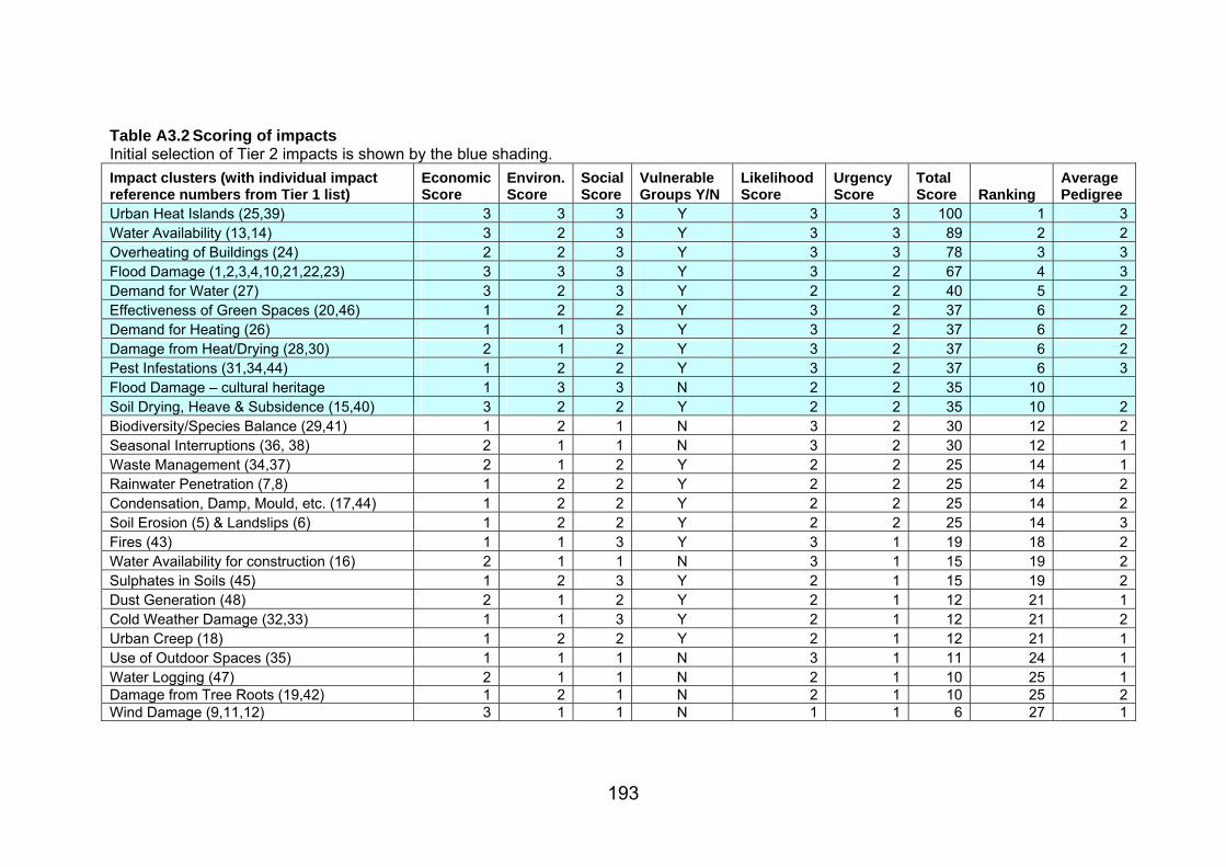
193
Table A3.2 Scoring of impacts Initial selection of Tier 2 impacts is shown by the blue shading.
Impact clusters (with individual impact reference numbers from Tier 1 list)
Economic Score
Environ. Score
Social Score
Vulnerable Groups Y/N
Likelihood Score
Urgency Score
Total Score Ranking
Average Pedigree
Urban Heat Islands (25,39) 3 3 3 Y 3 3 100 1 3 Water Availability (13,14) 3 2 3 Y 3 3 89 2 2 Overheating of Buildings (24) 2 2 3 Y 3 3 78 3 3 Flood Damage (1,2,3,4,10,21,22,23) 3 3 3 Y 3 2 67 4 3 Demand for Water (27) 3 2 3 Y 2 2 40 5 2 Effectiveness of Green Spaces (20,46) 1 2 2 Y 3 2 37 6 2 Demand for Heating (26) 1 1 3 Y 3 2 37 6 2 Damage from Heat/Drying (28,30) 2 1 2 Y 3 2 37 6 2 Pest Infestations (31,34,44) 1 2 2 Y 3 2 37 6 3 Flood Damage – cultural heritage 1 3 3 N 2 2 35 10 Soil Drying, Heave & Subsidence (15,40) 3 2 2 Y 2 2 35 10 2 Biodiversity/Species Balance (29,41) 1 2 1 N 3 2 30 12 2 Seasonal Interruptions (36, 38) 2 1 1 N 3 2 30 12 1 Waste Management (34,37) 2 1 2 Y 2 2 25 14 1 Rainwater Penetration (7,8) 1 2 2 Y 2 2 25 14 2 Condensation, Damp, Mould, etc. (17,44) 1 2 2 Y 2 2 25 14 2 Soil Erosion (5) & Landslips (6) 1 2 2 Y 2 2 25 14 3 Fires (43) 1 1 3 Y 3 1 19 18 2 Water Availability for construction (16) 2 1 1 N 3 1 15 19 2 Sulphates in Soils (45) 1 2 3 Y 2 1 15 19 2 Dust Generation (48) 2 1 2 Y 2 1 12 21 1 Cold Weather Damage (32,33) 1 1 3 Y 2 1 12 21 2 Urban Creep (18) 1 2 2 Y 2 1 12 21 1 Use of Outdoor Spaces (35) 1 1 1 N 3 1 11 24 1 Water Logging (47) 2 1 1 N 2 1 10 25 1 Damage from Tree Roots (19,42) 1 2 1 N 2 1 10 25 2 Wind Damage (9,11,12) 3 1 1 N 1 1 6 27 1

194

Built Environment sector 195
Appendix 4 Response Functions

196 Built Environment sector

197
BE2 – Subsidence
1. Determine estimated total number of dwellings at risk from subsidence a) Determine estimated land area by region of shrink-swell clays (derived from BGS map) b) Use number of dwellings as per Council Tax Bands (DCLG data) c) Assume ABI subsidence claims are distributed across regions in proportion to estimated dwellings at risk Total Land Area of GOR, Scotland and Wales
Land Area (km2) Estimated Area of significant shrink-swell clay soils (% of region)
Estimated Area with significant shrink-swell threat (km2)
Total number of dwellings by region
Estimated Dwellings at risk
Baseline: No of insurance claims for subsidence (ABI, 2009)
England 130,282 22,481,264 4,194,111 29,700 of which: East 19,109 35% 6,688 2,466,733 863,357 6,114 East Midlands 15,606 10% 1,561 1,927,013 192,701 1,365 London 1,572 75% 1,179 3,278,746 2,459,060 17,413 North East 8,573 NA 1,165,201 0 North West 14,107 NA 3,107,960 0 South East 19,071 15% 2,861 3,599,041 539,856 3,823 South West 23,837 5% 1,192 2,327,124 116,356 824 West Midlands 12,998 NA 2,331,286 0 Yorkshire & The Humber
15,408 1% 154 2,278,160 22,782 161
Scotland 77,932 NA 0 Wales 20,734 NA 1,348,900 0 Northern Ireland 13,562 NA Data Sources: Land Area: http://www.ons.gov.uk/about-statistics/geography/products/geog-products-other/sam/index.html Estimated Area of significant shrink-swell clay soils (% of region): http://www.bgs.ac.uk/products/geosure/pdf/shrink_swell.pdf (Figure 4.2) Total number of dwellings by region: DCLG: Dwelling Stock By Council Tax Band, 2008 Baseline: Number of insurance claims for subsidence, ABI: Domestic Subsidence - Gross Incurred Claims (ABI, 2009)
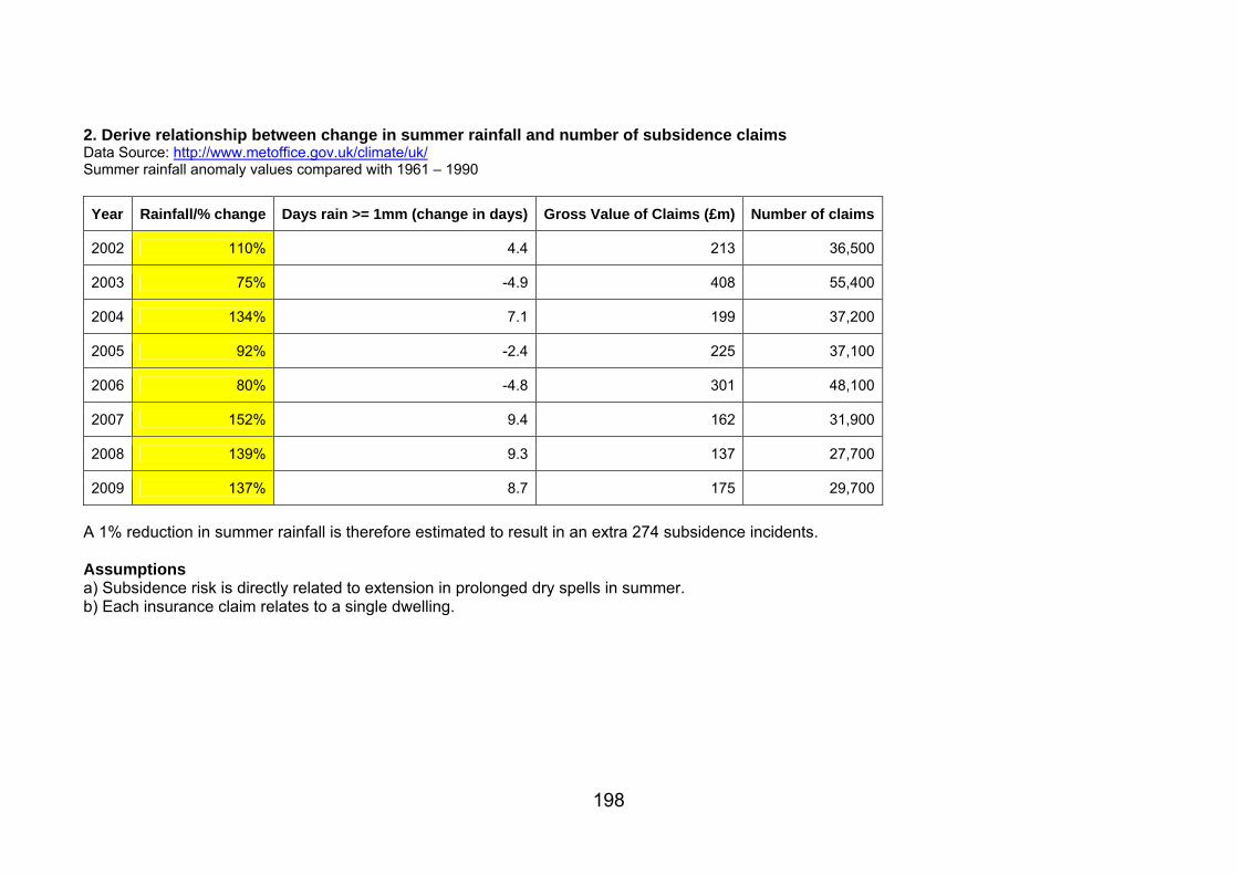
198
2. Derive relationship between change in summer rainfall and number of subsidence claims Data Source: http://www.metoffice.gov.uk/climate/uk/ Summer rainfall anomaly values compared with 1961 – 1990
Year Rainfall/% change Days rain >= 1mm (change in days) Gross Value of Claims (£m) Number of claims
2002 110% 4.4 213 36,500
2003 75% -4.9 408 55,400
2004 134% 7.1 199 37,200
2005 92% -2.4 225 37,100
2006 80% -4.8 301 48,100
2007 152% 9.4 162 31,900
2008 139% 9.3 137 27,700
2009 137% 8.7 175 29,700
A 1% reduction in summer rainfall is therefore estimated to result in an extra 274 subsidence incidents. Assumptions a) Subsidence risk is directly related to extension in prolonged dry spells in summer. b) Each insurance claim relates to a single dwelling.

Built Environment sector 199
BE3 – Overheating of Buildings
Data Source: Daily regional Tmax from Armstrong et al. (2010) dataset. Calculate average number of days per annum for which Tmax >= 26°C.
BE5 – Effectiveness of Green Space
Figure A4.1 Percentage change in effective green space versus relative aridity score (As Figure 4.6 but with reduction in effective green space expressed in percentage terms.)

200 Built Environment sector
BE9 - Demand for Heating
1. Calculate Baseline Regional Heating Degree Days Heating if Tmean < 15.5 °C Data Source: Met Office mean annual temperature data for period 1990 - 2009 2. Determine domestic energy consumption per household Source: High Level Energy Indicators 2007 (DECC, May 2010) Table 1.4
NUTS1 Code NUTS1 Region
Total domestic energy consumption/ household (kWh)
UKL Wales 21,320 UKM Scotland 21,620 UKC North East 21,550 UKD North West 21,390
UKE Yorkshire and the Humber 21,770
UKF East Midlands 20,950 UKG West Midlands 20,850 UKH East of England 20,150 UKI Greater London 19,870 UKJ South East 21,330
UKK South West 18,830
3. Determine proportion of this energy attributable to heating Source: Energy Consumption in the UK Overall Data Tables 2010 Update (DECC) Overall energy consumption for heat and other end uses by fuel 2008
Thousand tonnes of oil
equivalentSector End use Gas Oil Solid fuel Electricity Total
Domestic Space heating 21,887 2,305 596 1,455 26,244
Water heating 8,357 725 155 1,501 10,738
Cooking/catering 668 3 3 625 1,300 Heat total 30,913 3,033 753 3,582 38,282
Lighting and appliances 3 - - 7,236 7,239
Overall total 1 30,916 3,033 753 10,818 45,521 Space heating as proportion of total energy use 58%
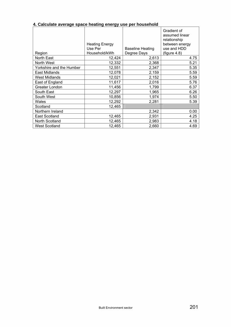
Built Environment sector 201
4. Calculate average space heating energy use per household
Region
Heating Energy Use Per Household/kWh
Baseline Heating Degree Days
Gradient of assumed linear relationship between energy use and HDD (figure 4.8)
North East 12,424 2,613 4.75North West 12,332 2,368 5.21Yorkshire and the Humber 12,551 2,347 5.35East Midlands 12,078 2,159 5.59West Midlands 12,021 2,152 5.59East of England 11,617 2,016 5.76Greater London 11,456 1,799 6.37South East 12,297 1,965 6.26South West 10,856 1,974 5.50Wales 12,292 2,281 5.39Scotland 12,465 Northern Ireland 2,342 0.00East Scotland 12,465 2,931 4.25North Scotland 12,465 2,983 4.18West Scotland 12,465 2,660 4.69

202 Built Environment sector

Built Environment sector 203
Appendix 5 Application of Climate Change Projections
BE2 – Subsidence
To apply climate change projections: UKCP09 projected percentage change in summer rainfall for given scenario and region used to calculate projected subsidence claims using relationship given in Figure 4.3.
BE3 – Overheating of Buildings
To apply climate change projections: UKCP09 projected average change in Tmax (for given scenario, region, season) added to baseline dataset (Daily regional Tmax from Armstrong et al., 2010). Calculate average number of days per annum for which Tmax >= 26°C.
BE5 – Effectiveness of Green Space
Table A5.1 Relative aridity scores for England and Wales
Low Emissions Medium Emission High Emissions
p10 p50 p90 p10 p50 p90 p10 p50 p90
2020s 0.49 1.00 1.55 0.49 1.03 1.61 0.51 1.02 1.58
2050s 0.87 1.59 2.41 1.05 1.82 2.71 1.20 2.03 2.98
2080s 1.11 1.96 2.97 1.53 2.54 3.75 1.94 3.14 4.58
Table A5.2 Reduction in Effectiveness of Green space (percentage reduction in total area)
2020s 2050s 2080s
Med
ium
Med
ium
Med
ium
Lo
w
Lo
w
Med
ium
Hig
h
Hig
h
Lo
w
Lo
w
Med
ium
Hig
h
Hig
h
2008 baseline p10 p50 p90 p10 p50 p50 p50 p90 p10 p50 p50 p50 p90
0.0 0.0 0.6 12.2 0.0 11.8 16.4 20.6 39.6 2.2 19.2 30.8 42.8 71.6
Using response function figure A4.1.

204
BE9 - Demand for Heating
Table A5.3 BE9 – Demand for Heating: Projected Change in Heating Degree Days (by region)
2020s 2050s 2080s
Medium Medium Medium Low Low Medium High High Low Low Medium High High
UKCP09 Region
1990 - 2009
baseline p10 p50 p90 p10 p50 p50 p50 p90 p10 p50 p50 p50 p90
East Midlands 2159 -167 -381 -592 -255 -543 -607 -684 -987 -397 -705 -805 -951 -1357
East of England 2016 -164 -367 -569 -248 -523 -585 -660 -949 -384 -679 -777 -915 -1305
London 1799 -153 -344 -535 -234 -492 -496 -621 -888 -360 -640 -732 -861 -1214
North East 2613 -150. -404 -664 -266 -578 -633 -805 -1047 -418 -749 -836 -994 -1448
North West 2368 -143 -351 -561 -180 -458 -515 -765 -881 -335 -630 -707 -855 -1252
South East 1965 -162 -369 -569 -248 -522 -548 -658 -950 -382 -680 -776 -917 -1301
South West 1974 -168 -369 -566 -240 -506 -568 -690 -912 -385 -663 -761 -892 -1259
West Midlands 2152 -173 -376 -581 -249 -524 -559 -703 -944 -398 -683 -785 -922 -1307
Yorkshire and The Humber 2347 -175 -403 -635 -271 -578 -661 -746 -1050 -420 -752 -860 -1015 -1453
Northern Ireland 2342 -54 -344 -625 -190 -501 -704 -793 -928 -309 -643 -685 -782 -1226
Wales 2281 -184 -398 -616 -260 -553 -645 -763 -996 -417 -723 -831 -975 -1379

205
2020s 2050s 2080s
Medium Medium Medium Low Low Medium High High Low Low Medium High High
UKCP09 Region
1990 - 2009
baseline p10 p50 p90 p10 p50 p50 p50 p90 p10 p50 p50 p50 p90
East Scotland 2931 -64 -375 -692 -210 -556 -586 -635 -1034 -339 -711 -755 -875 -1380
North Scotland 2983 -155 -423 -703 -278 -609 -601 -874 -1134 -437 -790 -896 -1071 -1584
West Scotland 2660 -152 -417 -682 -272 -594 -725 -838 -1081 -429 -772 -864 -1025 -1490
Isle of Man 2198 -135 -356 -584 -236 -510 -701 -617 -913 -369 -657 -733 -867 -1251
Heating if Tmean < 15.5°C Baseline Data Source: Met Office mean annual temperature data for period 1990 - 2009 As a proxy for projected heating degree days: The baseline daily mean average temperature is adjusted by the projected change in mean average winter temperature under each UKCP09 scenario. The adjusted 20-year series of mean daily temperatures is then used to calculate future heating degree days (against a heating temperature baseline of 15.5 deg C) and a 20 year average calculated.

206
Table A5.4 BE9 – Demand for Heating: Household Space Heating Energy Consumption
Household Space Heating Energy Consumption (‘000 GWh/yr) - including climate change
2020s 2050s 2080s
Medium Medium Medium Low Low Medium High High Low Low Medium High High
UKCP09 Region 2008 baseline p10 p50 p90 p10 p50 p50 p50 p90 p10 p50 p50 p50 p90
East Midlands 22 20.5 18 16 20 17 16 15 12 18 15 14 12 8
East of England 27.5 25 22.5 20 24 20 19.5 18.5 14.5 22 18 17 15 10
London 37 34 30 26 32 27 27 24 19 29 24 22 19 12
North East 13.5 13 11 10 12 10.5 10 9 8 11 10 9 8 6
North West 35 33 30 27 33 29 28 24 22 30 26 25 23 17
South East 42 39 34 30 37 31 30 28 22 34 28 25.5 22.5 14
South West 24 22 19 17 21 18 17 15.5 13 19 16 15 13 8.7
West Midlands 26.5 24 22 19 23.5 20 20 18 15 22 18 17 15 10
Yorkshire & The Humber 27 25 22 20 24 20.5 19.5 18.5 15 22 18.5 17 15 10
Northern Ireland 22 20.5 18 16 20 17 16 15 12 18 15 14 12 8
Wales 27.5 25 22.5 20 24 20 19.5 18.5 14.5 22 18 17 15 10
East Scotland 12 11 10 9 11 9 9 9 7.5 10 9 9 8 6
North Scotland 5 5 4 4 4.5 4 4 3.5 3 4 5 3.5 3 2
West Scotland 14 13 12 10 13 11 10 10 8 12 10 9 9 6
See Figure 4.8 for linear relationship between HDD and assumed energy use.
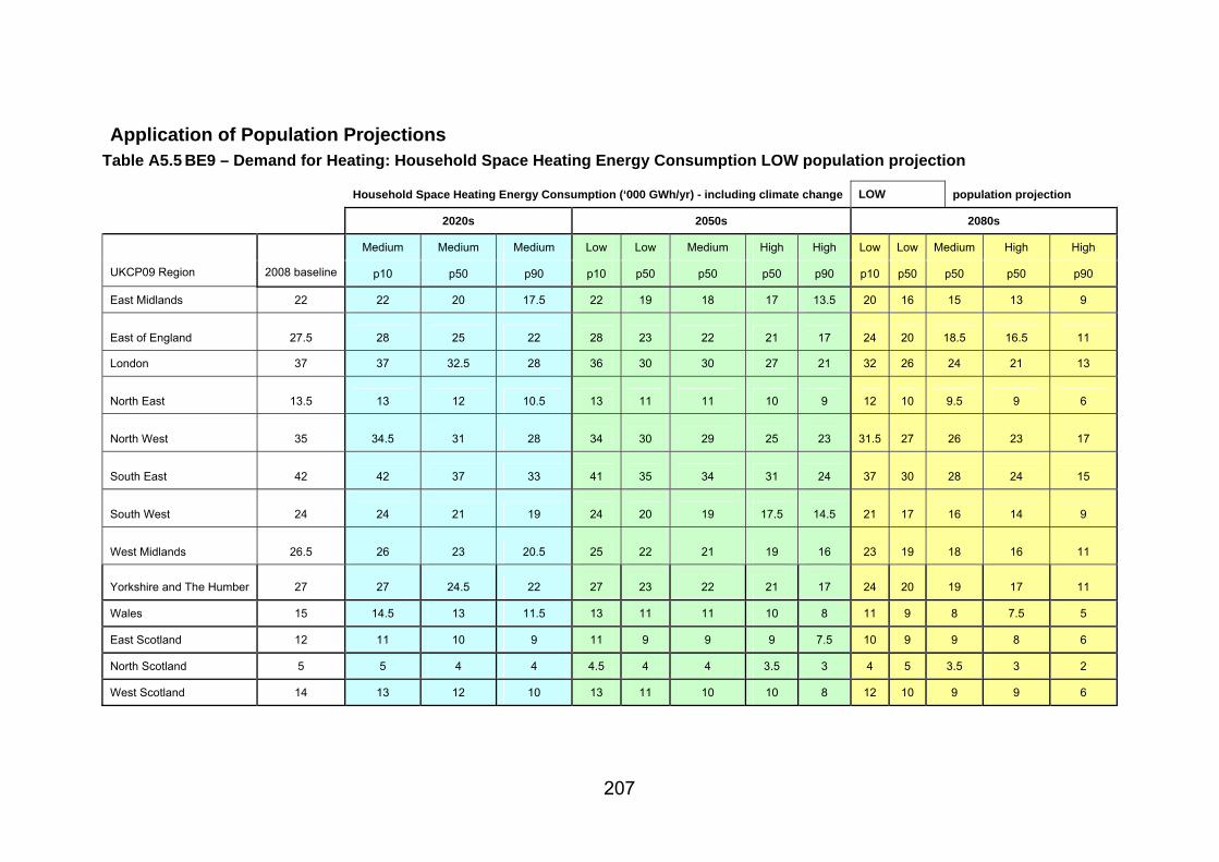
207
Application of Population Projections Table A5.5 BE9 – Demand for Heating: Household Space Heating Energy Consumption LOW population projection
Household Space Heating Energy Consumption (‘000 GWh/yr) - including climate change LOW population projection
2020s 2050s 2080s
Medium Medium Medium Low Low Medium High High Low Low Medium High High
UKCP09 Region 2008 baseline p10 p50 p90 p10 p50 p50 p50 p90 p10 p50 p50 p50 p90
East Midlands 22 22 20 17.5 22 19 18 17 13.5 20 16 15 13 9
East of England 27.5 28 25 22 28 23 22 21 17 24 20 18.5 16.5 11
London 37 37 32.5 28 36 30 30 27 21 32 26 24 21 13
North East 13.5 13 12 10.5 13 11 11 10 9 12 10 9.5 9 6
North West 35 34.5 31 28 34 30 29 25 23 31.5 27 26 23 17
South East 42 42 37 33 41 35 34 31 24 37 30 28 24 15
South West 24 24 21 19 24 20 19 17.5 14.5 21 17 16 14 9
West Midlands 26.5 26 23 20.5 25 22 21 19 16 23 19 18 16 11
Yorkshire and The Humber 27 27 24.5 22 27 23 22 21 17 24 20 19 17 11
Wales 15 14.5 13 11.5 13 11 11 10 8 11 9 8 7.5 5
East Scotland 12 11 10 9 11 9 9 9 7.5 10 9 9 8 6
North Scotland 5 5 4 4 4.5 4 4 3.5 3 4 5 3.5 3 2
West Scotland 14 13 12 10 13 11 10 10 8 12 10 9 9 6

208
Table A5.6 BE9 – Demand for Heating: Household Space Heating Energy Consumption PRINCIPAL population projection
Household Space Heating Energy Consumption (‘000 GWh/yr) – including climate change PRINCIPAL population projection
2020s 2050s 2080s
Medium Medium Medium Low Low Medium High High Low Low Medium High High
UKCP09 Region 2008 baseline p10 p50 p90 p10 p50 p50 p50 p90 p10 p50 p50 p50 p90
East Midlands 22 23 21 18 26 22 21 20 16 27 23 21 19 12
East of England 27.5 30 26 23 34 28.5 27 26 20 36 29 27 24 16
London 37 39 34 30 43 36 36 32 25 44.5 36 33 29 18
North East 13 14 12 11 14 12 12 11 9 14 12 11.5 10.5 7.5
North West 35 35 32 29 37.5 33 32 27 25 37 32 30 28 20
South East 42 44 39 34 49 41 40 37 29 51 41 38 34 21
South West 24 25 22 19.5 28 24 23 21 17 29 24 22 20 13
West Midlands 26.5 27 24 21 28.5 24 24 22 18 29 24 22 20 14
Yorkshire and The Humber 27 29 26 23 32 27.5 26 25 20 34 28 26 23 16
Wales 15 17 17 17 18 18 18 18 18 19 19 19 19 19
East Scotland 12 13 11 10 12 10.5 10 10 8 11.5 10 10 9 7
North Scotland 5 5 4 4 5 4 4 4 3 4 5 4 3 2
West Scotland 14 13 12 10.5 13 11 10 10 8 12 10 9.5 9 6

209
Table A5.7 BE9 – Demand for Heating: Household Space Heating Energy Consumption HIGH population projection
Household Space Heating Energy Consumption (‘000 GWh/yr) - including climate change HIGH population projection
2020s 2050s 2080s
Medium Medium Medium Low Low Medium High High Low Low Medium High High
UKCP09 Region 2008 baseline p10 p50 p90 p10 p50 p50 p50 p90 p10 p50 p50 p50 p90
East Midlands 22 24.5 22 19 31 26 25 24 19 36 30 28 25 16.5
East of England 27.5 31 28 24 40 34 33 31 24 49 0 37 33 21
London 37 40 36 31 50 42 42 38 29 59 47 44 38 24
North East 13 14 12.5 11 15.5 13.5 13 12 10 17 14 14 12.5 9
North West 35 36 33 29 41 35.5 34 30 28 43.5 37 35.5 32 24
South East 42 46 41 36 57 48 47 43 34 67 54 50 44 28
South West 24 26 23 20.5 33 28 27 24.5 20 39 32 30 26.5 17.5
West Midlands 26.5 27.5 25 22 32 27 27 24 20 35 30 28 25 17
Yorkshire and The Humber 27 30 27 24 38 32 31 29 24 45 37 35 31 21
Wales 15 16 14 13 19 16 15 14 12 21 18 16 15 10
East Scotland 12 14 12.5 11 13 12 11.5 11 9 13 11 11 10 8
North Scotland 5 5 4.5 4 5 4 4 4 3 4.5 5 4 3 2.5
West Scotland 14 13.5 12 11 13 11 10 10 8.5 12 10 10 9 6

210

Built Environment sector 211
Appendix 6 Monetisation
This section provides the full tables of values and supporting unit values.

212 Built Environment sector
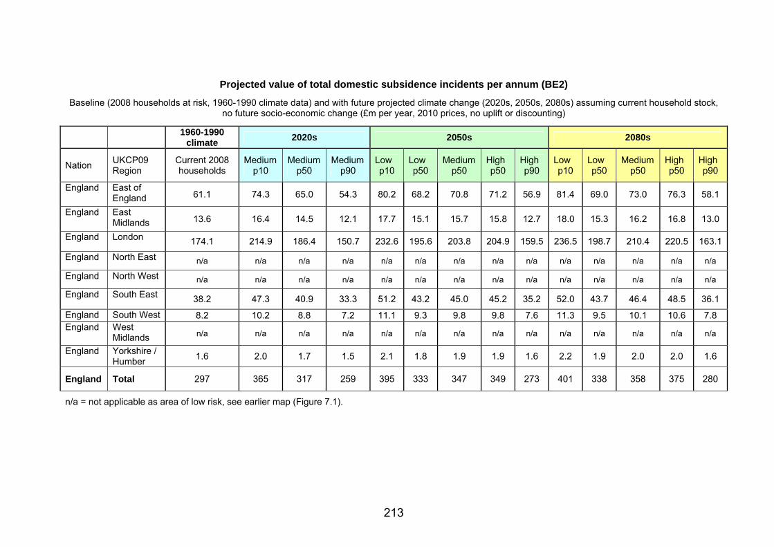
213
Projected value of total domestic subsidence incidents per annum (BE2)
Baseline (2008 households at risk, 1960-1990 climate data) and with future projected climate change (2020s, 2050s, 2080s) assuming current household stock, no future socio-economic change (£m per year, 2010 prices, no uplift or discounting)
1960-1990
climate 2020s 2050s 2080s
Nation UKCP09 Region
Current 2008 households
Medium p10
Medium p50
Medium p90
Low p10
Low p50
Medium p50
High p50
High p90
Low p10
Low p50
Medium p50
High p50
High p90
England East of England 61.1 74.3 65.0 54.3 80.2 68.2 70.8 71.2 56.9 81.4 69.0 73.0 76.3 58.1
England East Midlands 13.6 16.4 14.5 12.1 17.7 15.1 15.7 15.8 12.7 18.0 15.3 16.2 16.8 13.0
England London 174.1 214.9 186.4 150.7 232.6 195.6 203.8 204.9 159.5 236.5 198.7 210.4 220.5 163.1
England North East n/a n/a n/a n/a n/a n/a n/a n/a n/a n/a n/a n/a n/a n/a
England North West n/a n/a n/a n/a n/a n/a n/a n/a n/a n/a n/a n/a n/a n/a
England South East 38.2 47.3 40.9 33.3 51.2 43.2 45.0 45.2 35.2 52.0 43.7 46.4 48.5 36.1
England South West 8.2 10.2 8.8 7.2 11.1 9.3 9.8 9.8 7.6 11.3 9.5 10.1 10.6 7.8 England West
Midlands n/a n/a n/a n/a n/a n/a n/a n/a n/a n/a n/a n/a n/a n/a
England Yorkshire / Humber
1.6 2.0 1.7 1.5 2.1 1.8 1.9 1.9 1.6 2.2 1.9 2.0 2.0 1.6
England Total 297 365 317 259 395 333 347 349 273 401 338 358 375 280
n/a = not applicable as area of low risk, see earlier map (Figure 7.1).
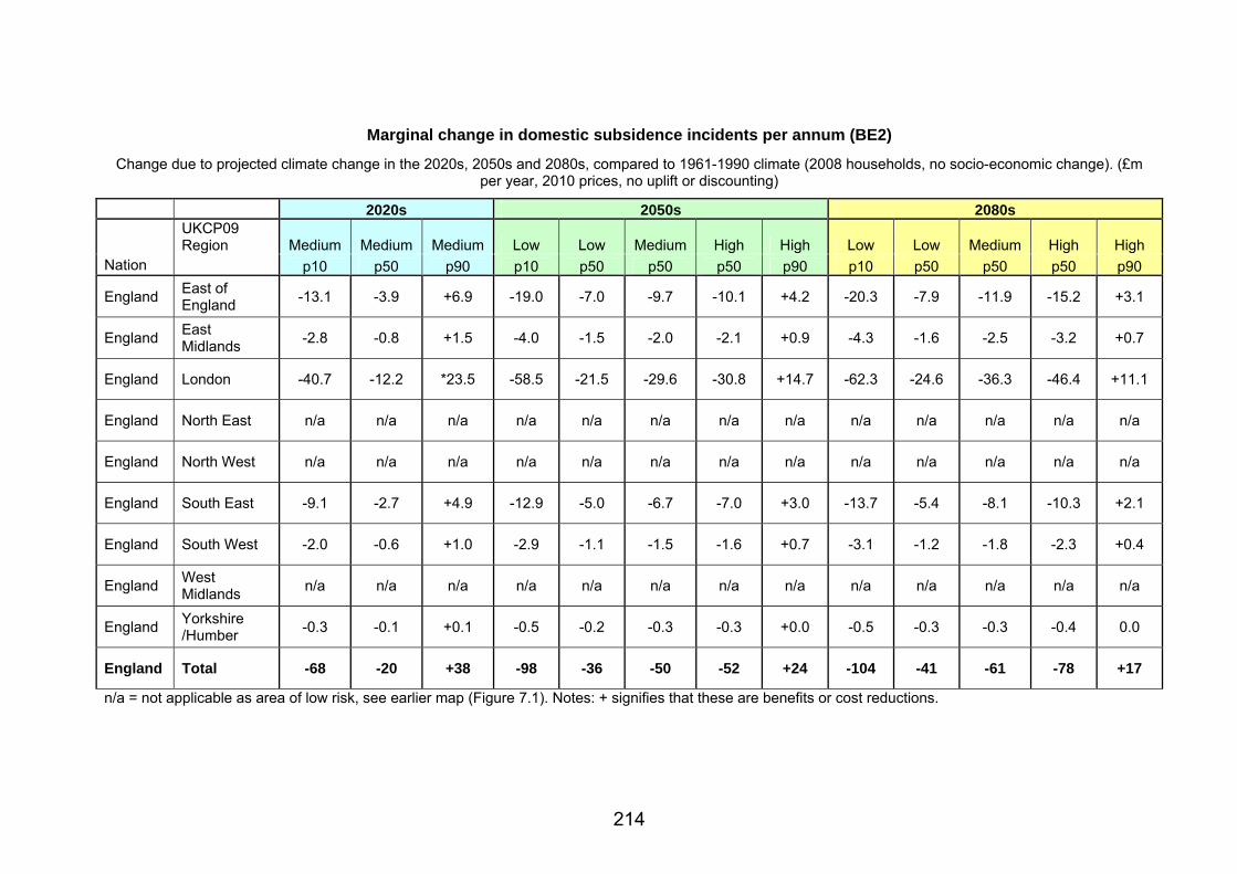
214
Marginal change in domestic subsidence incidents per annum (BE2)
Change due to projected climate change in the 2020s, 2050s and 2080s, compared to 1961-1990 climate (2008 households, no socio-economic change). (£m per year, 2010 prices, no uplift or discounting)
2020s 2050s 2080s UKCP09 Region Medium Medium Medium Low Low Medium High High Low Low Medium High High
Nation p10 p50 p90 p10 p50 p50 p50 p90 p10 p50 p50 p50 p90
England East of England
-13.1 -3.9 +6.9 -19.0 -7.0 -9.7 -10.1 +4.2 -20.3 -7.9 -11.9 -15.2 +3.1
England East Midlands
-2.8 -0.8 +1.5 -4.0 -1.5 -2.0 -2.1 +0.9 -4.3 -1.6 -2.5 -3.2 +0.7
England London -40.7 -12.2 *23.5 -58.5 -21.5 -29.6 -30.8 +14.7 -62.3 -24.6 -36.3 -46.4 +11.1
England North East n/a n/a n/a n/a n/a n/a n/a n/a n/a n/a n/a n/a n/a
England North West n/a n/a n/a n/a n/a n/a n/a n/a n/a n/a n/a n/a n/a
England South East -9.1 -2.7 +4.9 -12.9 -5.0 -6.7 -7.0 +3.0 -13.7 -5.4 -8.1 -10.3 +2.1
England South West -2.0 -0.6 +1.0 -2.9 -1.1 -1.5 -1.6 +0.7 -3.1 -1.2 -1.8 -2.3 +0.4
England West Midlands
n/a n/a n/a n/a n/a n/a n/a n/a n/a n/a n/a n/a n/a
England Yorkshire /Humber
-0.3 -0.1 +0.1 -0.5 -0.2 -0.3 -0.3 +0.0 -0.5 -0.3 -0.3 -0.4 0.0
England Total -68 -20 +38 -98 -36 -50 -52 +24 -104 -41 -61 -78 +17
n/a = not applicable as area of low risk, see earlier map (Figure 7.1). Notes: + signifies that these are benefits or cost reductions.

215
Future energy price projections. Source IAG and supplementary green book guidance on valuing energy use (2009 prices).
Note prices do not change in the period post 2050, thus are not shown.
Energy prices - Central 2010 Average 2020 2030 2040 Average 2050 2060 2070
2011-2040
2041-2070
ELECTRICITY - retail: domestic p/KWh (2009) 11.6 18.1 15.1 21.8 21.8 21.8 21.8 21.8 21.8
ELECTRICITY - retail: commercial p/KWh (2009) 10.0 16.8 13.6 20.8 20.8 20.8 20.8 20.8 20.8
ELECTRICITY - retail: industrial p/KWh (2009) 9.2 15.4 12.5 19.1 19.1 19.1 19.1 19.1 19.1
ELECTRICITY - Variable element: domestic p/KWh (2009) 7.4 11.2 8.6 14.0 14.0 14.0 14.0 14.0 14.0
ELECTRICITY - Variable element: commercial p/KWh (2009) 6.8 10.4 7.9 13.0 13.0 13.0 13.0 13.0 13.0
ELECTRICITY - Variable element: industrial p/KWh (2009) 6.4 9.7 7.4 12.1 12.1 12.1 12.1 12.1 12.1
GAS - retail: domestic p/KWh (2009) 3.7 5.1 5.1 5.5 5.5 5.5 5.5 5.5 5.5
GAS - retail: commercial p/KWh (2009) 2.9 3.9 4.0 4.3 4.3 4.3 4.3 4.3 4.3
GAS - retail: industrial p/KWh (2009) 2.6 3.6 3.6 3.9 3.9 3.9 3.9 3.9 3.9
GAS - Variable element: domestic p/KWh (2009) 2.2 2.7 2.5 2.9 2.9 2.9 2.9 2.9 2.9
GAS - Variable element: commercial p/KWh (2009) 2.1 2.5 2.4 2.7 2.7 2.7 2.7 2.7 2.7
GAS - Variable element: industrial p/KWh (2009) 2.1 2.5 2.4 2.7 2.7 2.7 2.7 2.7 2.7
Energy prices - Low 2010 Average 2020 2030 2040 Average 2050 2060 2070
2011-2040
2041-2070
ELECTRICITY - retail: domestic p/KWh (2009) 9.3 13.7 12.6 15.6 15.6 15.6 15.6 15.6 15.6
ELECTRICITY - retail: commercial p/KWh (2009) 7.6 12.2 11.0 14.4 14.4 14.4 14.4 14.4 14.4
ELECTRICITY - retail: industrial p/KWh (2009) 7.0 11.2 10.1 13.2 13.2 13.2 13.2 13.2 13.2
ELECTRICITY - Variable element: domestic p/KWh (2009) 5.1 6.2 5.4 7.0 7.0 7.0 7.0 7.0 7.0
ELECTRICITY - Variable element: commercial p/KWh (2009) 4.6 5.6 4.9 6.4 6.4 6.4 6.4 6.4 6.4
ELECTRICITY - Variable element: industrial p/KWh (2009) 4.3 5.3 4.6 6.0 6.0 6.0 6.0 6.0 6.0
GAS - retail: domestic p/KWh (2009) 2.8 3.8 4.0 4.1 4.1 4.1 4.1 4.1 4.1
GAS - retail: commercial p/KWh (2009) 1.9 2.6 2.7 2.8 2.8 2.8 2.8 2.8 2.8
GAS - retail: industrial p/KWh (2009) 1.7 2.3 2.5 2.5 2.5 2.5 2.5 2.5 2.5
GAS - Variable element: domestic p/KWh (2009) 1.3 1.4 1.4 1.5 1.5 1.5 1.5 1.5 1.5
GAS - Variable element: commercial p/KWh (2009) 1.2 1.2 1.2 1.3 1.3 1.3 1.3 1.3 1.3
GAS - Variable element: industrial p/KWh (2009) 1.2 1.2 1.2 1.3 1.3 1.3 1.3 1.3 1.3

216
Energy prices - High 2010 Average 2020 2030 2040 Average 2050 2060 2070
2011-2040
2041-2070
ELECTRICITY - retail: domestic p/KWh (2009) 12.7 20.5 16.9 24.9 24.9 24.9 24.9 24.9 24.9
ELECTRICITY - retail: commercial p/KWh (2009) 11.2 19.3 15.5 24.0 24.0 24.0 24.0 24.0 24.0
ELECTRICITY - retail: industrial p/KWh (2009) 10.2 17.7 14.2 22.0 22.0 22.0 22.0 22.0 22.0
ELECTRICITY - Variable element: domestic p/KWh (2009) 8.5 13.4 11.0 16.3 16.3 16.3 16.3 16.3 16.3
ELECTRICITY - Variable element: commercial p/KWh (2009) 7.8 12.4 10.1 15.1 15.1 15.1 15.1 15.1 15.1
ELECTRICITY - Variable element: industrial p/KWh (2009) 7.3 11.6 9.5 14.1 14.1 14.1 14.1 14.1 14.1
GAS - retail: domestic p/KWh (2009) 4.2 5.9 6.2 6.3 6.3 6.3 6.3 6.3 6.3
GAS - retail: commercial p/KWh (2009) 3.3 4.8 5.1 5.1 5.1 5.1 5.1 5.1 5.1
GAS - retail: industrial p/KWh (2009) 3.1 4.4 4.7 4.7 4.7 4.7 4.7 4.7 4.7
GAS - Variable element: domestic p/KWh (2009) 2.6 3.5 3.6 3.6 3.6 3.6 3.6 3.6 3.6
GAS - Variable element: commercial p/KWh (2009) 2.5 3.3 3.4 3.4 3.4 3.4 3.4 3.4 3.4
GAS - Variable element: industrial p/KWh (2009) 2.5 3.3 3.4 3.4 3.4 3.4 3.4 3.4 3.4
Energy prices - High High 2010 Average 2020 2030 2040 Average 2050 2060 2070
2011-2040
2041-2070
ELECTRICITY - retail: domestic p/KWh (2009) 14.2 23.1 18.7 27.9 27.9 27.9 27.9 27.9 27.9
ELECTRICITY - retail: commercial p/KWh (2009) 12.7 22.0 17.3 27.1 27.1 27.1 27.1 27.1 27.1
ELECTRICITY - retail: industrial p/KWh (2009) 11.6 20.2 15.9 24.8 24.8 24.8 24.8 24.8 24.8
ELECTRICITY - Variable element: domestic p/KWh (2009) 9.8 15.9 13.1 18.8 18.8 18.8 18.8 18.8 18.8
ELECTRICITY - Variable element: commercial p/KWh (2009) 9.1 14.8 12.1 17.4 17.4 17.4 17.4 17.4 17.4
ELECTRICITY - Variable element: industrial p/KWh (2009) 8.5 13.8 11.3 16.3 16.3 16.3 16.3 16.3 16.3
GAS - retail: domestic p/KWh (2009) 4.7 6.7 7.0 7.1 7.1 7.1 7.1 7.1 7.1
GAS - retail: commercial p/KWh (2009) 3.9 5.7 6.0 6.0 6.0 6.0 6.0 6.0 6.0
GAS - retail: industrial p/KWh (2009) 3.6 5.2 5.4 5.5 5.5 5.5 5.5 5.5 5.5
GAS - Variable element: domestic p/KWh (2009) 3.1 4.3 4.3 4.4 4.4 4.4 4.4 4.4 4.4
GAS - Variable element: commercial p/KWh (2009) 3.0 4.1 4.2 4.2 4.2 4.2 4.2 4.2 4.2
GAS - Variable element: industrial p/KWh (2009) 3.0 4.1 4.2 4.2 4.2 4.2 4.2 4.2 4.2
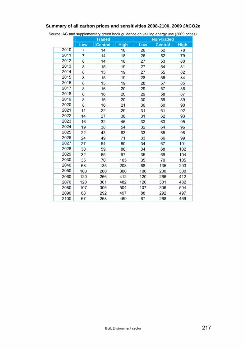
Built Environment sector 217
Summary of all carbon prices and sensitivities 2008-2100, 2009 £/tCO2e
Source IAG and supplementary green book guidance on valuing energy use (2009 prices).
Traded Non-traded Low Central High Low Central High 2010 7 14 18 26 52 78 2011 7 14 18 26 52 79 2012 8 14 18 27 53 80 2013 8 15 19 27 54 81 2014 8 15 19 27 55 82 2015 8 15 19 28 56 84 2016 8 15 19 28 57 85 2017 8 16 20 29 57 86 2018 8 16 20 29 58 87 2019 8 16 20 30 59 89 2020 8 16 21 30 60 90 2021 11 22 29 31 61 92 2022 14 27 38 31 62 93 2023 16 32 46 32 63 95 2024 19 38 54 32 64 96 2025 22 43 63 33 65 98 2026 24 49 71 33 66 99 2027 27 54 80 34 67 101 2028 30 59 88 34 68 102 2029 32 65 97 35 69 104 2030 35 70 105 35 70 105 2040 68 135 203 68 135 203 2050 100 200 300 100 200 300 2060 120 266 412 120 266 412 2070 120 301 482 120 301 482 2080 107 306 504 107 306 504 2090 88 292 497 88 292 497 2100 67 268 469 67 268 469

218 Built Environment sector
Projected value for total domestic space heating per annum (BE9) - (£Billion) with future energy price projections
Baseline (2008 households at risk, 1960-1990 climate data) with FUTURE prices based on 2010 Energy Price projections central (£m per year, 2009 prices, no uplift or discounting) 1) future climate change (2020s, 2050s, 2080s) assuming current household stock, no future socio-economic change 2) for socio-economic only (no climate change) 3) with climate change and socio-economic change (household growth). See earlier text for caveats.
£Billion /year (with FUTURE energy prices)
1) Socio-economic change only (population and household alone) central socio-economic, central energy projections (no climate change)
2010 2020s 2050s 2080s
England 5.53 7.64 9.46 10.90
2) Climate change only, current socio-economic, central energy projections
2010 2020s 2050s 2080s
Medp10
Medp50
Medp90
Lowp10
Lowp50
Medp50
Hghp50
Hghp90
Lowp10
Lowp50
Medp50
Hghp50
Hghp90
England 5.53 6.26 5.58 4.92 6.46 5.50 5.34 4.90 4.01 5.97 4.94 4.61 4.12 2.76
3) Climate change and Socio-Economic Change (central) together, Central energy projections
Medp10
Medp50
Medp90
Lowp10
Lowp50
Medp50
Hghp50
Hghp90
Lowp10
Lowp50
Medp50
Hghp50
Hghp90
England 5.53 7.04 6.28 5.53 8.36 7.11 6.90 6.34 5.17 8.64 7.13 6.65 5.93 3.95