Climate change

Prediction

Data collection and presentation by

Carl Denef, Januari 2014

1

Climate models Climate models are simplified numerical representations of the climate system

constructed with two types of essential building blocks: physical, chemical, and biological principles founded on theory (the laws of thermodynamics and Newton’s laws of motion, for example) and data collected from observations on climate system components. The basic models, known as General Circulation Models (GCM), handle 3-dimentional circulation dynamics of the atmosphere and ocean through mathematical equations. The Earth’s surface is represented in a grid of millions of stacked cubes, with each representing a specific area of land, ocean, sea ice, and atmosphere (see Figure next slide). Each cube is a collection of mathematical formulas describing the processes within that area. The mathematical equations are numerically solved by super-computers that calculate as accurately as possible what will happen to temperatures, winds, water currents, and many other parameters in each cube under various scenarios. For instance, models resolve the question of what happens to temperature after a doubling of the current atmospheric CO2 concentration. The cubes are then joined to calculate how circulation in one cube will interact with that in surrounding grids and integrated over the globe. Resolution of the grid cells is between 300 and 30 km. The higher the resolution the longer the computer time needed. Even with the best supercomputers of today, calculation times can extend over several weeks. At present, climate projections are based on an ensemble of different models, known as multi-model ensembles. The reason for this is that averages across different models show better large-scale agreement with observations.

2

Climate models are used to simulate global and regional climate variability and change over past periods, to project changes in the near future (decadal scale) and to predict changes over longer periods (century scale). They potentially provide valuable guidance to help policy makers and businesses adapt to and mitigate climate change.

3

Reliability of climate models has to be tested against what happened with

climate in the past.[125] If a model can correctly simulate trends from a particular starting point somewhere in the past, it can be used to predict with reasonable certainty what might happen in the future. However, different models include different entry elements and may therefore generate different predictions. Results can also vary due to different greenhouse gas or aerosol inputs, the model's climate sensitivity to greenhouse gases (= the change in temperature upon doubling of CO2 in the atmosphere), the use of differing estimates of future greenhouse gas emissions (for example the rate of methane leakage during shale gas extraction) and so on. A model-based prediction is therefore presented under different scenarios with respect to humanity’s future demographic expansion and behavior. Which scenarios are most realistic is uncertain, as the projections of future greenhouse gas and aerosol emission are themselves uncertain.

Certain processes represented in the model may be too complex or too small-scale to be physically represented in the model. In that case the process is replaced by a simplified process. This manipulation is known as parameterization. Various parameters are used in these simplified processes. An example are clouds. Cloud formation is notoriously complex and climate model gridboxes for clouds have a resolution of 5 km, which is much larger than the scale of a typical cumulus cloud (1 km). Therefore the processes that such clouds represent are parameterized.

Because of simplification by parameterization and uncertainty in scenarios, climate models always enclose estimates of uncertainty levels.

4

Climate system elements used in climate models

Source: Nature 463, 747-756 (11 February 2010)

Clouds

5

Reliability of climate models Models have accurately predicted climate change trends in the past. For

example, the vulcanic eruption of Mt. Pinatubo allowed to test the accuracy of models by entering the eruption data and then observe how climate changed. The observed climatic response was found consistent with the prediction. Predictions of atmospheric CO2 levels made by IPCC in 1990 were also fully confirmed by the later observations (see slides on ‘Climate change in the atmosphere’). Models also correctly predicted greater warming in the Arctic and over land, greater warming at night, and stratospheric cooling.

Other predictions underestimated climate change, such as arctic ice melting and sea level rise predicted by the IPCC Third Assessment report. Precipitation rates also increased significantly faster than global climate models predicted.

Still others slightly over-estimated the rise in atmospheric methane concentrations (see IPCC AR5 WG1).

An important uncertainty factor in climate predictions is climate sensitivity – being the temperature response to a doubling of the atmospheric greenhouse gas concentration –, because it is affected by climate feedbacks. Higher climate sensitivity will result in more warming, in case of a positive feedback.[Ref] If a negative feedback is acting, a given greenhouse gas rise will result in less sensitivity.

Climate models are still not well predicting the effect of clouds [Ref] , due to lack in knowledge of cloud generation processes. Uncertainties in methane release from permafrost and leakage during methane extraction from shale gas by fracking, are other examples of prediction uncertainties.

6

Climate sensitivity Projections of climate change in the future are dependent on the sensitivity of the

climate system to the greenhouse radiative forcing. It is therefore essential to have an accurate estimate of this sensitivity. Climate sensitivity is a measure of the surface temperature change in °C per W/m2 sustained radiative forcing. In practice it is expressed as the temperature change associated with a doubling of the concentration of CO2 in the atmosphere relative to pre-industrial levels (~280 ppm). There are two ways to look at climate senstivity: equilibrium climate sensitivity (ECS) and transient climate sensitivity (TCS). The former is calculated over the time span needed to reach full equilibrium between sustained CO2 forcing and the climate system. TCS is defined as the average temperature response over a 20-year period to CO2 doubling with CO2 increasing at 1% per year.[Ref] TCS is lower than ECS, due to the "inertia" (slowliness) of ocean heat uptake and ice sheet feedbacks. Doubling CO2 level results in forcing of 3.7 W/m2. In a simple physical environment a doubling of CO2 would result in 1 °C warming. However, in the real atmosphere complex positive and negative feedbacks are operating (water vapor, cloud and ice albedo, aerosols, ozone…), influencing radiative forcing. The net warming effect was found to be ~3 times higher. Feedbacks can also become stronger with time. For example ice sheets may melt at a given time point at a much faster rate due to a sudden collapse of large ice shelves allowing massive release of ice into the sea. Icebergs drift away to warmer water and melt, hereby decreasing albedo, resulting in more warming. Addition of these longterm feedbacks to climate models was found to lead to a higher value of ECS, but most climate models have not included these feedbacks yet. Thus, future climate change may be more deleterious than presently expected.

7

Current climate models span an ECS range of 2.6–4.1 °C, most clustering

around 3 °C."[Ref] The IPCC AR5 concensus value of ECS, calculated by multimodel ensembles, is between 1.5°C and 4.5°C, is extremely unlikely <1°C, and very unlikely >6°C. Notice that feedback contribution, being not constant over time, induces a level of uncertainty in any climate model.

8

IPCC radiative forcing scenarios IPCC AR5 introduced a new set of scenarios, to project future climate

change with climate model simulations. These scenarios are called RCPs (Representative Concentration Pathways). These are based on the radiative forcing that emission rates would cause in the years to come. The main RCPs are RCP2.6, RCP4.5, RCP6.0, and RCP8.5, named after the radiative forcing values that are projected for the year 2100 i.e. +2.6, +4.5, +6.0, and +8.5 W/m2, respectively.[2]

In the RCP8.5 scenario radiative forcing is set to reach 8.5 W/m2 by 2100 and to continue to rise for some time thereafter. RCP6.0 and RCP4.5 are intermediate “stabilization pathways”, where radiative forcing does not further rise after 2100. In the RCP2.6 scenario, radiative forcing peaks at 3 W/m2 before 2050 and then declines to 2.6 by 2100.

To each forcing scenario there is a corresponding greenhouse gas level in the atmosphere (see next slides). In order to remain within this future greenhouse gas concentrations adopted in the RCP scenarios, the maximum cumulative fossil fuel emissions should be not higher than 272 Gt, 780 Gt, 1062 Gt and 1687 Gt carbon equivalents up to 2100 for RCP2.6, RCP4.5, RCP6.0, and RCP8.5, respectively (see next slides).

9

Although theoretically possible, [Ref]

RCP2.6 is a scenario difficult to attain, since 1) in 2012 radiative forcing was already 2.9 W/m2, 2) to realize RCP2.6, atmospheric CO2 must be stabilized at 450 ppm (see next slide) which requires a ~70% reduction of CO2 emissions relative to the level in 2000 (see section 5). 3) Both RCP2.6 and 4.5 scenarios already include ‘carbon dioxide removal’ (CDR) programs (see section 5) to remain within the radiative forcing limit and these CDR programs are presently considered difficult to realize on a sufficient global scale and with sufficient safety.

Trends in radiative forcing for 4 different scenarios (IPCC RCP scenarios). Forcing is relative to pre-industrial values and does not include land use (albedo), dust, or nitrate aerosol forcing (van Vuuren 2011).

Source

RCP8.5

RCP6.0

RCP4.5

RCP2.6

10

The Figures below show the greenhouse gas levels and maximum emissions

for the different RCP forcings.

Yearly carbon emissions allowed to meet each of the 4 RCP’ scenarios (mean +/- SD) (IPCC AR5 Figure 6.25)

Gt c

arbo

n/ye

ar

RCP 2.6

RCP 6.0

RCP 4.5

RCP 8.5

Greenhouse gas concentrations, expressed as atmospheric CO2-equivalent concentrations (ppm), corresponding to each RCP scenario up to 2100.

CO2-e

q. (p

pm)

11

Global surface temperature predictions In 2001 the IPCC third assessment report (TAR) announced that, although

the climate system was so complex, scientists would never reach complete certainty about present and future climate change, but that it is ‘much more likely than not’ that our civilization faces severe global warming

Since 2001, greatly improved computer models and an abundance of data have strengthened the IPCC conclusion. The IPCC conclusions were endorsed by national science academies of major nations and leading scientific societies.

In 2007 the IPCC fourth assessment report (AR4) stated that “it is ‘very likely’ that significant global warming is coming in our lifetimes. This surely brings a likelihood of harm, widespread and grave. Depending on what will be done to restrict emissions, we could expect the planet’s average surface temperature to rise anywhere between about 1.4-5.8°C by the end of this century.” Notice that the lower bound is already reached today!

The IPCC fifth assessment report (AR5), presented in September 2013 in Stockholm, projects a somewhat lower rise in global surface temperature in 2100. Increase of global mean surface temperatures for 2081–2100 relative to 1986–2005 is projected to ‘likely be’ in the range of 0.3 - 1.7°C (RCP2.6 scenario), 1.1 - 2.6°C (RCP4.5 scenario), 1.4 - 3.1°C (RCP6.0 scenario), or 2.6 - 4.8°C (RCP8.5 scenario). Notice that temperature during the reference period 1986–2005 had already risen by ~0.6 °C relative to the preindustrial temperature.

12

IPCC AR5 reported that “it is virtually certain that there will be more

frequent hot and fewer cold temperature extremes over most land areas on daily and seasonal timescales as global mean temperatures increase. It is very likely that heat waves will occur with a higher frequency and duration. Occasional cold winter extremes will continue to occur”

The Figure shows multimodel simulations for future global surface temperature under different RCP scenarios. Values are relative to 1985-2005. Numbers inside the Figure indicate the number of different models used for the different time periods.

(Figure 12.40 from IPCC AR5)Year

13

Land vs sea and seasonal differences Depending on the scenario considered, global average temperature on land

surface is anticipated to rise up to 6 °C, relative to averaged 1986–2005 temperatures, by 2100, with little difference between Winter and Summer. Sea surface temperature will rise as well but ~2°C less.

The Figures only show land temperatures. Thin lines denote one of 5 ensemble members per model, thick lines the CMIP5 multi-model mean. From IPCC AR5 Figure AI.4 and AI.5

14

Incidence of warm and cold days Warm days will drastically increase in number while cold days will decrease. The

Figure shows results from CMIP5 models under the RCP2.6, RCP4.5 and RCP8.5 scenarios.

From IPCC AR5 Figure 11.1715

Regional differences In certain regions surface temperature anomaly for

2080-2099 is expected to rise up to 10 °C, particulatly in the Arctic, threatening massive melting of Greenland ice sheets. Land surface will warm more than ocean.

The Figure (from IPCC AR5) shows the average surface temperature for the scenarios RCP2.6 and RCP8.5 in 2081– 2100 relative to 1986–2005, as calculated by CMIP5 multi-models. The number of CMIP5 models used is indicated in the upper right corner of each panel.

See NOAA animation video h e r e, showing the projected annual mean surface temperature regional distribution from 1970-2100, (credit: NOAA Geophysical Fluid Dynamics Laboratory).

16

Arctic region (67.5°–90° North) Depending on the RPC scenario examined, the Arctic will warm up to 3 x more

during Winter than during Summer. The sea surface tends to warm more than land surface, at least in Winter.

Land

Sea

December-Februari (Winter)

The Figure shows CMIP5 multi-model expectations of average temperature changes in Arctic areas up to 2100, relative to averaged 1986–2005 temperatures. From IPCC AR5 Figure AI.8 and AI9.

June-August (Summer)

Land

Sea

17

Antarctic region Temperature rise over land in Antarctica is much smaller than in the Arctic and

there is little difference between Winter and Summer.

December-Februari (Summer)

IPCC AR5 Figure A1.76 and 77

June-August (Winter)

Land Land

The Figure shows CMIP5 multi-model axpectations of average temperature changes in Arctic areas up to 2100, relative to averaged 1986–2005 temperatures.. From IPCC AR5 Figure AI.8 and AI9.

18

Land ice IPCC AR5 concluded that it is “ ‘exceptionally unlikely’ that the ice sheets of

either Greenland or West Antarctica will suffer a near-complete disintegration during the 21st century.” However, it may happen at a millenial time scale, because both the ocean and the ice masses are huge, which makes it very long before heat and CO2 of the surrounding atmosphere equilibrates. Moreover, as summarized by IPCC AR5 WG1 chapt. 13, models project that the Greenland Ice Sheet will exhibit a strongly nonlinear and potentially irreversible response to surface warming. The mechanism of this threshold behavior is the surface mass balance (SMB) height feedback, that is, as the surface height is lowered due to ice loss, the higher temperature above the near surface leads to further ice loss. This feedback is small in the 21st century but will become important in the 22nd century. This nonlinear behaviour may be accelerated by a reduced surface albedo caused by the continuous loss of ice sheet extent. Models have calculated a threshold in surface warming beyond which self-amplifying feedbacks result in a partial or near complete ice loss on Greenland. If a temperature above this threshold is maintained over a multi-millennial time period, the majority of the Greenland Ice Sheet will be lost on a millennial to multi-millennial time scale. The treshhold global mean surface temperature rise to initiate this evolution has been estimated to be 3.1 (1.9 to 4.6) °C above pre-industrial level. Other models found this threshold at a 2.5°C rise.

Look the summarizing video from NASA19

Consistent with this result is that during the Middle Pliocene warm intervals,

when global mean temperature was 2°C–3.5°C higher than pre-industrial, ice-sheet models calculated near-complete deglaciation of Greenland. Some scientists predict that climate change may make the entire Greenland ice sheet melt in about 2,000 years.[2] That alone would add 7m to sea level [3].

The surface mass balance of the Antarctic Ice Sheet is projected to increase in most models because increased snowfall outweighs melt increase. However, ice-shelf decay due to oceanic or atmospheric warming might lead to abruptly accelerated ice flow and loss into the sea. It remains uncertain whether East Antarctic ice sheet will gain or loose mass [Ref]

Also James Hansen has argued that multiple positive feedbacks could lead to nonlinear ice sheet disintegration by increased ice flow, calving and sudden ice shelve collapses. More surface melt water would flow to the ice sheet bed, leading to much faster melting of the ice interior.[Ref]. Moreover, as ice sheets shed ice more and more rapidly, in ice streams, climate simulations indicate that a point will be reached when the high latitude ocean surface cools while low latitudes surfaces are warming. Larger temperature contrast between low and high latitudes will drive more powerful storms.20

Arctic and Antarctic sea ice According to IPCC AR5 arctic sea ice will have virtually disappeared (< 1

km2 in extent) by 2050 (37 models with RCP8.5 scenario). Antarctic sea ice extent is also expected to decrease, altough at a considerably slower rate. Decreased sea ice extent means less albedo and thus faster warming.

From IPCC AR5 Figure 12.28

Changes in sea ice extent as simulated by CMIP5 models over the second half of the 20th century and the whole 21st century under RCP2.6, RCP4.5, RCP6.0 and RCP8.5 scenarios. The number of models used for each RCP is given in the legend. 21

Permafrost Permafrost area is expected to decrease with 15 million km2 in the worst case

scenario by 2100. Under sustained Arctic warming, models indicate with medium agreement that permafrost destabilization could cause a release of greenhouse gases up to 200 Gt CO2 equivalents (CO2 + methane) by 2100. This would cause substantial additional warming (see IPCC AR5 FAQ 6.2). However, an insufficient understanding of the relevant soil processes during and after permafrost thaw, precludes making a high confidence and precise projection. Of course, uncertainty does not guarantee safety.

The Figure below shows the trends in permafrost area under different RCP scenarios. Thick lines are multi-model average. Shading and thin lines indicate the inter-model spread (one standard deviation).

From IPCC AR5 Figure 12.33

22

Snow cover extent In all RCP scenarios Northern Hemisphere snow cover extent is anticipated

to decrease, resulting in reduced albedo and further warming. From IPCC AR5 Figure 12.32

Northern Hemisphere spring (March to April average) snow cover extent change (in %) in the CMIP5 model ensemble, relative to the simulated extent for the 1986–2005 reference period.

23

Methane clathrate destabilization Model simulations suggest that methane from terrestrial and oceanic

methane clathrate deposits in shallow ocean regions at high latitude and in the Gulf of Mexico are susceptible to destabilization by ocean warming. However, sea level rise will also increase ocean mass, which enhances clathrate stability (due to higher pressure by water). A net increase of methane release and a positive feedback on warming is expected over multi-millennial timescales.

A pertinent issue here is the threshold at which warming begins to mobilize seabed methane. Reaching this threshold would initiate a “runaway” feedback warming that characterized the PETM and EECO palaeoclimate periods. No one knows what the threshold is. Once warming is at that treshhold, methane will enter the atmosphere and give additional warming, which then will release more methane that then, in turn, gives warming and so on. Runaway warming is possible and, at that stage, uncontrollable.

24

Sea level rise Sea level rise is expected to continue

for centuries, even millenia, even when anthropogenic carbon emissions would stabilize at the present level[13] This is because the sea level contribution from ice sheets continues over these time scales. In 2007, the IPCC AR4 projected that during the 21st century, sea level will rise another 18 to 59 cm, but these numbers do not include "uncertainties in climate-carbon cycle feedbacks nor do they include the full effects of changes in ice sheet flow".[Ref] As shown in the Figure, IPCC AR5 predicts similar sea level rise. Projections assessed by the US National Research Council[Ref] suggest possible sea level rise over the 21st century of between 56 cm and 2 m. The predicted upper limit of sea level rise remains highly uncertain, due to the incomplete understanding of fast ice streams and glacier collapse that are major contributors of ice delivery to the sea and sea level rise (See Nature 461, 971-975, 2009).

25

Ultimate sea level rise In a recent article in PNAS (July 15, 2013), a

combination of palaeoclimate data with simulations by models was used to estimate the future sea-level commitment on a multimillennial time scale. It was found that oceanic thermal expansion and the Antarctic Ice Sheet will contribute quasi-linearly, with 0.4 m/°C and 1.2 m/°C of warming, respectively. The contribution from glaciers saturates earlier while the response of the Greenland Ice Sheet is nonlinear. As a consequence sea-level rise is committed to approximately 2.3 m/°C within the next 2,000 years. Since a rise in temperature of at least 4 °C, relative to 1990, is expected by 2100 under a worst case scenario, at least a 10 m rise in global sea level is expected within 2 millennia even when no further rise in temperature would occur.

ocean warming

mountain glaciers

Greenland ice sheet

Antarctic ice sheet

total sea level

The Figure shows modelled Sea level rise contributions over the next 2000 years from: ocean warming (a), mountain glaciers (b), Greenland (c) and Antarctic (d) ice sheets, plotted against temperature rise from 1 to 4 °C. The total sea level rise (e) is about 2.3m per °C of warming above pre-industrial.

26

The PNAS paper also calculated the regional differences of sea level rise under a 1, 2, 3 and 4 °C sustained temperature rise (see Figure). Even under the « safe » 2 °C temperature rise, many regions in the World will see a 5-6 m sea level rise

The theoretical maximal sea level rise would be reached if all land ice would melt. According to IPCC AR4 this is 7 m if Greenland ice melts and 57 m if Antarctic Ice Sheets melt. Greenland melting alone would inundate most coastal cities over the world. The total possible contribution of glaciers (i.e., all of the land ice excluding the ice sheets) is limited to ∼0.5-0.6 m (From IPCC AR5, Ch. 4 and ref 22 in PNAS).

27

Ocean acidification The average pH of ocean surface waters today

has fallen by about 0.1 unit (from about 8.2 to 8.1) since 1765 and will further fall to 7.7 by the end of this century under the RCP8.5 scenario. To illustrate the potential damage to life and ecosystems, look at what happens to human cells during acidosis. The normal pH in human blood ranges between 7.35 and 7.45. Irreversible cell damage occurs when pH falls below 6.8 or rises above 7.8. However, it remains uncertain how much and how fast pH could change to allow ecosystems in the ocean to adapt.

Notice that under normal seawater conditions, the hydrogen ions that are produced from CO2 dissolved in water will combine with carbonate ion (CO3

2– ) to produce HCO3–. Doubling of CO2

levels in the atmosphere relative to preindustial levels would reduce carbonate ion concentration from 228 to 144 µmol/kg (IPCC AR5 FAQ 3.2, Table 1). Thus, uptake of anthropogenic CO2 into the oceans consumes carbonate ions, lowering availability of the building blocks of skeletons and shells in marine organisms.

From IPCC AR5 Figure 6.28

28

Ocean oxygen content About three O2 molecules are lost every time a single CO2 molecule is produced

by fossil fuel combustion. A 0.0317% decline in atmospheric oxygen has been recorded thus far (for the period 1990 to 2008) and is expected to drop further, as a consequence of the warming-induced decline in dissolved oxygen in the ocean upper 500 m. A second cause is the slowing down of the thermohaline circulation, resulting in less oxygen carried from the surface layers of the water into the deeper layers. Oxygen is the most important limiting factor on the growth of many marine organisms. Lowering oxygen makes it more difficult for these animals to find food, avoid predators, and reproduce.

From IPCC AR5 Figure 6.30

Simulated changes in dissolved O2 (mean and model range as shading) relative to 1990s for RCP2.6,RCP4.5, RCP6.0 and RCP8.5.

Multi-model simulated changes in dissolved O2 (mmol/m3) for 2090-2100 period relative to the 1990s for RCP8.5

29

Thermohaline circulation Thermohaline circulation is a major driver of climate. As reported by IPCC

AR5, it is very likely that the thermohaline circulation will weaken over the 21st century relative to preindustrial values. Weakening could occur as a consequence of high freshwater runoff from rapidly melting Greenland ice sheet. The weakening in 2100 is projected to be about 20–30% for the RCP4.5 scenario and 36–44% for the RCP8.5 scenario. The consequence will be cooling of the Atlantic Northern Hemisphere, as weakening of the thermohaline circulation diminishes the influx of warm tropical water into the northern Atlantic Ocean. Western Europe would then experience cold winters.

30

Water cycle IPCC AR5 projects a poleward movement of evaporated water by extratropical

winds, and a further increase of evaporation from the surface. At high latitudes there will be more rain, because a warmer atmosphere will allow greater precipitation. Subtropical areas likely will get drier. Upward motion in the Hadley circulation will promote tropical rainfall, while suppressing subtropical rainfall. Hadley circulation will shift its downward branch poleward (North and South) with associated drying.

According to the World Meteorological Organization the western United States and Mexico, the Mediterranean basin, northern China, Southern Africa, Australia, and parts of South America are other regions highly likely to experience harsh drought conditions in the future (9).

From IPCC AR5 FAQ 12.2, Figure 131

32

Look at the video animation of global rainfall by NASA-Goddard Space Flight Center Scientific Visualization Studio

The video shows the frequency that regions receive no rain (brown), moderate rain (tan), and very heavy rain (blue). The occurrence of no rain and heavy rain will increase, while moderate rainfall will decrease.

Global and regional precipitation change Multimodel projections show a positive trend in global precipitation (from

October to March) over land and over sea, but it is relatively small even under the worst case scenario RCP8.5. Higher latitude and tropical regions will experience the highest precipitation increases. Subtropical zones will be drier.

Land (Oct-March)

Sea (Oct-March)

From IPCC AR5 Figure AI.6; From IPCC AR5 Figure 12.2233

Wettest days incidence Extreme precipitation events will become more pronounced.

From IPCC AR5 Figure 11.17 From IPCC AR5 Figure 12.26

34

Monsoon circulation and precipitation The major monsoon systems are the West African and the Asian-Australian

monsoons. Warming-related changes in large-scale circulation influence the strength and extent of the overall monsoon circulation. Several studies show an intensification of the rainfall associated with the Indian summer monsoon, concomitant with a weakening of the summer monsoon circulation. In addition, anthropogenic land use change and atmospheric aerosol loading can lower the land-sea temperature difference and hence further weaken the monsoon circulation. The net effect is more precipitation, due to enhanced moisture transport into the monsoon regions.

For many people in India it is the variability of rainfall on shorter time scales that will have the biggest impacts. Intense heavy rainfall may lead to flooding while breaks in the monsoon of a week or more, may lead to water shortage and agricultural drought.

From IPCC AR5 FAQ 14.2, Figure 1

35

Extreme weather events

From IPCC ‘Special Report on Managing the Risks of Extreme Events and Disasters (SREX)’. 36

Temperature extremes It is virtually certain

that there will be more hot and fewer cold extremes by the end of this century. The temperature of the coldest day of the year will undergo larger increases than the warmest day (up to 7 °C and in many regions up to 11 °C), paricularly in the northern hemisphere at higher latitudes.

Multi-model projections of changes in the annual minimum of the minimum daily temperature and annual maximum of maximum daily temperature, (relative to a 1981–2000 reference period) under the RCP8.5 scenario. IPCC AR5 Figure 12.1337

There will be up to 7-

25 frost days (below 0°C) less by 2100, depending on the scenario considered. On the other hand, the number of tropical nights (above 20°C) will go up with 60 in the worst case scenario. The fall in frost days will be more pronounced at higher latitudes in the Northen Hemisphere, while tropical nights will increase most at tropical and subtropical latitudes (in some areas up to 90 days).

There will be more record high than record cold temperatures. Meehl et al. (2009) calculated that the current ratio of 2 to 1 for record daily maxima to record daily minima temperatures in the United States will become approximately 20 to 1 by the mid 21st century and 50 to 1 by late century.

IPCC AR5 Figure 12.13

38

Returning rare temperature extremes Climate models found large increases in the magnitude of rare extreme

temperatures (annual maximum and minimum daily average surface temperatures) that occur once in 20 year (or with a 5% chance every year). Larger changes are expected over land than over sea. In certain regions the warm temperature extremes could be 10 °C hotter while the cold temperature extremes could be 12 °C less cold.

From IPCC AR5 Figure 12.14

39

Humid heat waves Human discomfort, morbidity and mortality during heat waves depend not only on

temperature but also specific humidity. Coastal regions display abundant atmospheric moisture and therefore are expected to experience the greatest heat stress changes.In mediteranian areas the number of combined tropical nights and hot days per year will drastically increase.

From European Environment Agency40

Droughts Consecutive dry days will increase in number, particularly in North and

South Africa, South America, Southern Europe and Australia.

While previous long-term droughts in Southwest North America arose from natural causes, climate models project that this region will undergo progressive aridification as part of a general drying and poleward expansion of the subtropical dry zones caused by global warming.

Data are multimodel average changes in the period 2081-2100 relative to the 1981–2000 reference period. From IPCC AR5 Figure 12.26

41

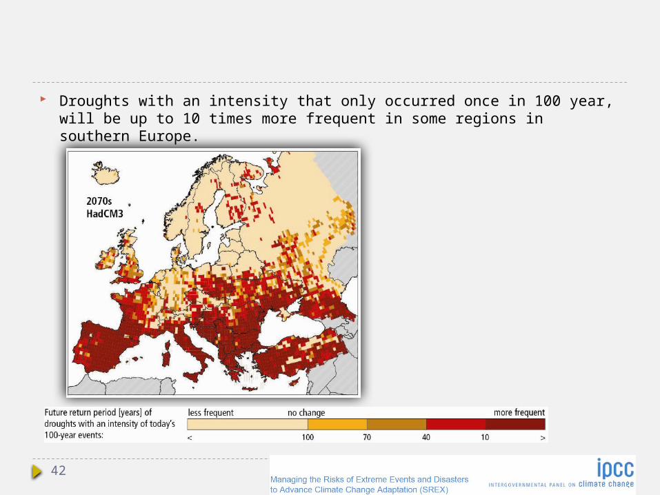
Droughts with an intensity that only occurred once in 100 year, will be up to

10 times more frequent in some regions in southern Europe.

42

Tropical cyclones The intensity of Atlantic hurricanes is expected to increase as the ocean

warms. More heat means more energy to drive atmospheric circulations, evaporation and ocean-air interactions. Although there have been dramatic improvements in predicting the trajectory of tropical cyclones, the largest uncertainty exists in the prediction of tropical cyclone intensity. The frequency of category 4 and 5 tropical cyclones over the 21st century is expected to increase, the largest increase projected to occur in the Western Atlantic, North of 20 degrees[Science 327, 454–458 (2010)]. A doubling of atmospheric CO2 may increase the frequency of the most intense cyclones [J. Clim. 17, 3477

(2004)].

On the other hand, there is evidence that the strong cyclones cause a large amount of ocean mixingRef, pumping heat from the surface down into the oceanic interior, which is then redistributed over the globe, particularly through upwelling of the heat in the equatorial Eastern Pacific, where El Niño originates. This may turn the globe into a permanent El Niño condition[Ref], which will favor global warming in a closed positive feedback loop.

In combination with sea level rise and tides, storm surges may cause more floods.

Moreover, climate simulations indicate that, as ice sheets release ice more and more rapidly in ice streams and hence cool the ocean at high latitude, a point will be reached when the high latitude ocean surface cools while low latitudes surfaces are warming. Larger temperature contrast between low and high latitudes will induce more powerful storms.[Ref]

43

Millenial scale projections of global warming and CO2 residence time It is very likely that large fractions of emitted CO2 will remain in the

atmosphere for at least 1000 years after anthropogenic emissions have stopped. Temperature will remain elevated for an even longer time due to the very slow mixing of heat with the deep ocean waters and the slow transfer of already stored heat in the oceans back into the atmosphere. This extremely long inertia times makes climate change irreversible on time scales relevant to human life (see next slide and IPCC AR5 Box 6.1).

There is high agreement between models that ocean warming and circulation changes will reduce the rate of CO2 uptake in the Southern Ocean and North Atlantic, which will amplify warming.

44

This Figure shows model-

simulated millenial evolution, under the 4 RCP scenarios, of atmospheric CO2 levels and global mean surface temperature after CO2 emissions up to 2300, followed by zero emissions after 2300,.

45

ppm

From IPCC AR5 Figure 12.44 adapted.The drop in temperature in 2300 is a result of eliminating all CO2 emissions. Shadings and bars denote the minimum to maximum range. The dashed line on panel (b) indicates the pre-industrial CO2 concentration.

This Figure shows model-

simulated changes of global mean surface temperature and atmospheric CO2 levels up to the year 3000, under the 4 RCP forcing scenarios, up to 2300 followed by a constant (year 2300 level) radiative forcing (Zickfeld et al., 2013). Under RCP8.5, radiation will reach 12.5 W/m2 by 2300. Notice that CO2 will rise to 7 x preindustrial, and average temperature will be 8 °C higher. Shadings and bars denote the minimum to maximum range. The dashed line on panel (a) indicates the pre-industrial CO2 concentration.

Other models predict a temperature increase above 8 °C by 2300 (see IPCC AR5 Figure 12.40).

From IPCC AR5 Figure 12.43

46

Is the World inhabitable with a 10 °C rise in average global temperature? The human body at rest cannot survive in an ambient sustained wet bulb

temperature (Tw) ≥35°C. The highest Tw (Twmax) anywhere on Earth today is ~30 °C and the most-common Twmax is 26–27 °C.[Ref] About 58% of the world’s population in 2005 resided in regions where Twmax ≥ 26 °C. A recent climate model simulation study reported that a global average temperature rise of 5 °C would result in a Twmax > 35 °C in some locations. [Ref] For an 8.5 °C increase the most-common value of Twmax would be 35 °C , which is incompatible with human life. With a 10 °C rise, many regions would experience a Tw = 35 °C at a particular time each year, even in Siberia (see next slide). It looks therefore that most of the World would be practically inhabitable in a 10 °C warmer climate. At this temperature grain and agricultural production would suffer very much or be destroyed, causing a food crisis. Humans could air-condition their houses but deployment this over the World will be economically and energetically extremely demanding and a power failure would be life threatening. People working outside cannot work in air-conditioned environments and these would rapidly develop hyperthermia. Poorer countries, which are located in tropical and subtropical regions, will be hit the most.

During the PETM and EECO average global surface temperature rose 7-14 °C, which is comparable to the study mentioned above. The question is then: How life could have adapted to that hothouse? Humans have a body temperature of 37 °C but many other mammals have a 2 °C and birds a 5 °C warmer body temperature[Ref] [Ref].

47

Non-human mammals and birds therefore may be more heat-tolerant than humans. Just before the onset of the PETM mammals were small-sized (average = 1 kg)[Ref] [Ref] [Ref]). This may have allowed their survival at that time, as small body mass is better adapted to high temperatures (higher surface/mass ratio allowing better cooling). Bioevolution during the PETM occurred over a time span of 20,000 years. In contrast, anthropogenic warming extends over a few centuries, too short for a significant evolutionary adaptation in heat tolerance.

But is this a realistic scenario? RCP8.5 is considered by IPCC as a worst case scenario maintained up to 2300. If this scenario becomes reality, humans will have made the World ~5-10 °C warmer by then. Atmospheric concentration would have risen to ~7 x preindustrial. If fossil fuel burning would further increase, we would be on the way to a 10 °C rise. However, it looks highly unlikely that humans would not reduce greenhouse gas emissions as soon as the impacts of climate change become frightening, which is definitely earlier than 2300. Nonetheless, the temperatures reached at that time would decrease only very slowly, even under strong reductions or complete elimination of CO2 emissions. Temperature might even increase temporarily due to an abrupt reduction of short-lived aerosol emissions and, hence, of aerosol negative forcing – see IPCC AR5 Ch. 12). Heat stored in the ocean will be released at an even slower rate. Thus, we would be forced to live in a World with climate disasters in many regions for many centuries.

48

Can a 10 °C rise be reached if we burn all fossil energy?

Since it takes more than 1000 years for emitted CO2 to be removed, the cumulative amount of emitted CO2 determines future climate. The amount of fossil fuels still available ranges between 7,300-15,000 gigatonnes carbon equivalent. James Hansen calculated[Ref] that burning this amount would increase Earth’s average surface temperature with 16°C. It would make the World practically inhabitable.

49

Source

The Figure shows the distribution of global average temperature (T), wet-bulb temperature (Tw) and maximum Tw (Twmax) on land from 60°South to 60°North during the decade 1999–2008 (upper panel) and the model-simulated distribution of these values for a 10 °C increased surface temperature (lower panel). The dotted red line in the lower panel is the model-simulated distribution under the present surface temperature. Notice the

Observations today

50

good agreement between observations and model. On the right side it can be seen that large parts of the World will experience a Twmax of 35 °C or more at periods during the year (panel F).

Permanent departure from climate variability In a recent paper in the journal Nature (Nature 502, 183–187) the year at

which the climate will exceed the bounds of its historical variability was calculated, using Earth system models. Under the RCP4.5 scenario, the global surface temperature average will have risen beyond historical variability by 2069, i.e. 56 years from now. Under the RCP8.5 scenario, this will be in 2047 i.e. within 34 years from now. Furthermore, after 2050 most tropical regions are expected to have every subsequent month lying outside of their historical range of variability. This means that every month will be an extreme climatic record. Ocean pH is already permanently outside its historical variability range. The same paper found that the Tropics will be the earliest to experience historically unprecedented climates, probably because the relatively small natural climate variability in the Tropics, which makes that climate bounds are easily surpassed by relatively small climate changes. Such small but fast changes could induce considerable biological damage. Studies in corals, terrestrial ectoderms, plants and insects show that tropical species live in areas with climates near their physiological tolerances and are therefore vulnerable to relatively small climate changes. These are alarming results, because most of the world’s biodiversity is concentrated in the Tropics. The situation will be further impaired because protection and mitigation initiatives are limited in the Tropics due to the lack of economical power of most countries in these regions. 51

These findings have enormous consequences on human society because

under RCP4.5 conditions roughly 1 billion people will live in areas where climate will exceed historical bounds of variability by 2050 and these people have no historical responsibility for the climate changes. Under RCP8.5 conditions this will be 5 billion people.

52

Ecosystems[Ref]

In terrestrial ecosystems, the earlier timing of spring events, and poleward and upward shifts in plant and animal range, have been linked with high confidence to recent warming. Future climate change is expected to particularly affect certain ecosystems, including tundra, mangroves, and coral reefs. It is expected that most ecosystems will be affected by higher atmospheric CO2 levels, combined with higher global temperatures. Overall, it is expected that climate change will result in the extinction of many species and reduce ecosystems diversity. Since ecosystems provide many goods and services to humans and other living systems in a mutually dependent manner, the consequences of ecosystem losses may become a very serious problem.

The current rate of ocean acidification is many times faster than at least the past 300 million years, which included four mass extinctions that involved rising ocean acidity, such as the Permian mass extinction, which killed 95% of marine species. By the end of the century, acidity changes would match that of the Palaeocene-Eocene Thermal Maximum (see slides on palaeoclimate), which occurred over 5000 years and killed 35–50% of benthic foraminifera[Ref] . It has been shown that corals, coccolithophore algae, coralline algae, foraminifera, shellfish and pteropods experience reduced calcification when exposed to elevated CO2 in the oceans. [Ref]

Warming of the surface ocean, combined with ocean acidification and reduction in ocean oxygen concentration will have potentially nonlinear multiplicative impacts on biodiversity and ecosystems and each may increase the vulnerability of ocean

53

systems, triggering an extreme impact. In the upper 500 m of the oceans oxygen levels range between 50 and 300 mmol/m3, with levels highest at higher latitudes. [Ref] Many marine organisms cannot survive under hypoxic conditions (oxygen between 60 to 120 mmol/m3 depending on the species).[Ref] [Ref] Multiple studies reported an impressive increase in the number of hypoxic ocean zones and their extension, severity, and duration.[Ref] There are several examples in palaeoclimate records that extreme ocean hypoxia led to the loss of 90% of marine animal taxa.[Ref] The slowing down of the ocean’s circulation also results in fewer nutrients from the deep layers into the ocean surface, which endangers oxygen-producing phytoplankton that live in the ocean surface. Phytoplankton organisms produce half of the world’s oxygen output (the other half is produced by plants on land). Hence, with decreasing numbers of these oxygen producers, the level of oxygen in the ocean is bound to decline further, entailing dramatic shortages in food supply. As reported by the IPCC AR5 WG1 chapt. 12, models consistently predict an increase in dry season length, and a 70% reduction in the areal extent of the rainforest by the end of the 21st century under a worst case scenario. If the dry season becomes too long, wildfires combined with human-caused fire ignition, can undermine the forest’s resiliency. Fire and deforestation could act as a trigger to abruptly and irreversibly change the forest ecosystem. Forests purify our air, improve water quality, keep soils intact, provide us with food, wood products and medicines, protect

54

against heat, and are home to many of the world’s most endangered species. An estimated 1.6 billion people worldwide rely on forests for their livelihoods, including 60 million indigenous people who depend on forests for their subsistence. Forests also help protect the Planet from climate change by absorbing massive amounts of CO2. Boreal forests could tip into a different vegetation state under climate warming. It should be noted, however, that uncertainties on the likelihood of it are very high, due to large gaps in knowledge of the ecosystemic and plant physiological responses to warming (see IPCC AR5 WG1 chapt. 12).

55

Look at a movie on plant productivity decrease despite more CO2 availability

Socio-economic consequences Water and food supply:

Ocean warming, oxygen depletion, and acidification will result in reduction in primary productivity of living species and, hence, in ocean goods and services for humans. More floods will destroy more crops. Less water means less agriculture, food and income. Crop yield will be decreased in drier areas. The Himalayan glaciers provide water for drinking, irrigation, and other uses for about 1.5 billion people. Since most glaciers in the Hindu Kush Himalayan region are retreating, the concern has been raised that over time the region's water supply may be threatened. However, recent studies show that at lower elevations, glacial retreat is unlikely to cause significant changes in water availability over the next several decades. Other factors, such as groundwater depletion and increasing water use by human activity could have a greater impact than the decrease of glacier water. On the other hand, higher elevation areas could experience less water flow in some rivers if current rates of glacier retreat continue, but shifts in rain and snow due to climate change will likely have a greater impact on regional water supplies[Ref] . Whatever the reason, climate change may likely threaten water supply and consequently food supply. Glacier recession reduces the buffering role of glaciers, hence inducing more floods during the rainy season and more water shortages during the dry season.

56

Human health:

Climate change caused >100,000 deaths/year at present. By 2030, climate change is estimated to indirectly cause nearly one million deaths a year and inflict 157 billion dollars in damage in terms of today's economy. Read more hereDiseases that are caused by prolonged exposure to heat include cramps, fainting, and heatstroke, and these can eventually lead to death. The key to preventing such health hazards is the accessibility of air conditioning. But as heat extremes will become more common, the reliance on air conditioning could cause problems for people in areas that are both adapted to high temperatures and those that are not. In regions like the southern United States, which are today accustomed to heat and where air conditioning is common, the increasing demands on power generators could become problematic if heat waves increase. In the Northwestern United States and Europe, where few places have air conditioning today, problems include making air conditioning available and ensuring that there is enough power to supply them. An important inherent factor deteriorating human health is that emissions inherently cause pollution and pollutants caused 400,000 premature deaths in Europe alone.

57

Increased exposure to tropical cyclones. The most exposed regions to

tropical cyclones are the U.S. and East-Asia (88% of all tropical cyclones). According to Yale and MIT researchers in a paper published in Nature Climate Change, tropical cyclones will cause $109 billion in damages by 2100,.

58

Increased exposure to floods.

An increase in the frequency or intensity of floods would be catastrophic in many low-lying places around the World. Asian countries are particularly at risk, as low-lying areas (like river deltas and small islands) are densely populated. In Bangladesh alone, over 17 million people live at an elevation of less than 1 m above sea level, and millions more inhabit the flat banks of the Ganges and Brahmaputra Rivers. Another consideration is that poorer countries like Bangladesh do not have the financial resources to relocate their citizens to lower risk areas, nor are they able to create protective barriers. Read more

The Organization for Economic Co-Operation and Development announced the 10 cities most vulnerable to flooding. Six are in Asia: Mumbai, Shanghai, Ho Chi Minh City, Calcutta, Osaka, and Guangzhou. The other four are in the United States: New York City, Miami, Alexandria, and New Orleans. All are coastal, low-lying, and densely populated[12].

Floodwaters can contaminate drinking water, and sea level rise can lead to the contamination of private wells, with local catastrophic results.

59

In Asia the number of people exposed to floods will increase from 29 million

in 1970 to 77 million in 2030

60

Hotspots for vulnerability

River Deltas and megadeltas are highly vulnerable to the impacts of climate change, particularly sea-level rise and changes in river runoff. Many of them also experience strong urban area expansion, collecting more and more people in small land spots. A global sample of 40 deltas inhabited by ~300 million people was studied for the impact of climate change. This analysis showed that much of the population of these 40 deltas is at risk through coastal erosion and land loss, primarily as a result of decreased sediment delivery by the rivers (due to the effects of water use and diversion, and declining sediment input as a consequence of water entrapment in dams). This phenomenon of land subsidence augments relative sea-level rise. Many people are already subject to flooding from both storm surges and seasonal river floods.

61

62

Relative vulnerability of coastal deltas in terms of the number of people potentially displaced by current sea-level trends to 2050 (Extreme = >1 million; High = 1 million to 50,000; Medium = 50,000 to 5,000; following Ericson et al., 2006). From IPCC “Climate Change 2007: Impacts, Adaptation and Vulnerability”, Chapter 6

Transport infrastructure

Transport infrastructure is vulnerable to extremes in temperature, floods from precipitation and rivers, and storm surges.

Since 80 % of global trade in goods is transported by sea, freight-handling ports and their road and rail connections, will be at high risk for serious damage from storm surges and floods, particularly in regions with very low elevation above sea level such as the U.S. Gulf Coast.

63

Heat waves can cause road pavement to soften and expand and can place stress on bridge joints. Heat waves or floods can also limit construction activities, particularly in areas with high humidity. With these changes, it could become more costly to build and maintain roads and highways.

Storms and floods may damage oil pipe lines and cause oil spills.

64

Impacts on tourism (from IPCC, Managing the Risks of Extreme Events

and Disasters to Advance Climate Change Adaptation) (SREX). These include:

Direct impacts on tourist infrastructure (hotels, access roads, etc.), on operating costs (heating/cooling, snowmaking, irrigation, food and water supply, evacuation, and insurance costs), on emergency preparedness requirements, and on business disruption (e.g., sun-and-sea or winter sports holidays)

Indirect environmental change impacts of extreme events on biodiversity and landscape (e.g. coastal erosion), which may negatively affect the quality and attractiveness of tourism destinations

Adverse weather conditions or the occurrence of an extreme event can reduce a touristic region’s popularity during the following season.

65

Environmental refugees:

There are currently between 25-30 million refugees worldwide as a consequence of climate events, and their numbers are expected to rise to 200 million by 2100.[14]Unlike traditional refugees, environmental refugees are not recognized by the Geneva Convention or the United Nations High Commission on Refugees (UNHCR), and therefore do not have the same legal status in the international community. Most threatened are people in developing countries - in particular, people in low-lying regions, on small islands, and arid regions that suffer from drought across North Africa, farm regions dependent on river water from glacier and snow melt, and regions of Southeast Asia facing changes in monsoon patterns. These countries have the least economical power to adapt to climate change. Most international statements on human rights in relation to climate change have emphasized the potential adverse impacts of climate change on the human rights to life, health, food, water, housing, development, and self-determination.[13] These rights are enumerated in the UN conventions of international human rights law, though not all UN members or UNFCCC parties have signed these conventions.

66

Worsening of human conflicts.

The impact of climate change will make the poorest communities across the world poorer. Many of them experience conflict and instability, on top of poverty, which exposes them to a dual risk. The impact of climate change may entail more violent conflict, which in turn counteracts governments and people to adapt to climate change. Thus, climate change and violent conflict create a potential vicious circle of destruction, if not properly cared of by the international community.

International peacebuilding NGO International Alert named 46 countries where climate change effects may interact with economic, social, and political forces to create a high risk of violent conflict.[15]

1. Afghanistan2. Algeria3. Angola4. Bangladesh5. Bolivia6. Bosnia & Herzegovina7. Burma8. Burundi9. Central African Republic10. Chad11. Colombia12. Congo13. Côte d’Ivoire14. Dem. Rep. Congo15. Djibouti16. Eritrea17. Ethiopia18. Ghana19. Guinea20. Guinea Bissau21. Haiti22. India23. Indonesia24. Iran

25. Iraq26. Israel & Occupied Territories27. Jordan28. Lebanon29. Liberia30. Nepal31. Nigeria32. Pakistan33. Peru34. Philippines35. Rwanda36. Senegal37. Sierra Leone38. Solomon Islands39. Somalia40. Somaliland41. Sri Lanka42. Sudan43. Syria44. Uganda45. Uzbekistan46. Zimbabwe

67

Combined climate change impacts (Europe)

The Figure shows predictions (using CCLM models under an IPCC scenario between RCP6.0 and RCP8.5) of climate change impacts for the period 2070-2100, based on regional sensitivity and exposure to climate factors and with a weighted combination of physical, environmental, social, economical and cultural impact parameters. From IRPUD Espon Climate Project, 2011 ©

68

Potentially abrupt and irreversible changes (”tipping points”) According to IPCC AR5 WG1 Chapter 12, abrupt climate change is defined

as a large-scale change in the climate system that develops over a few decades or less, persists for at least a few decades, and causes substantial disruptions in human and natural systems. Abrupt changes arise from nonlinearities within the climate system. They are therefore inherently difficult to assess and their timing is difficult to predict. Nevertheless, progress is being made on the basis of early warning signs for abrupt climate change.

AR5 defines a perturbed climate state as irreversible (also known as a “tipping point”), if the timescale of recovery from this state via natural processes is significantly longer than the time it took for the climate system to reach this perturbed state. According to this definition climate change resulting from CO2 emissions are irreversible, due to the long residence time of the CO2 in the atmosphere and the inertia of oceans to store the CO2 and the resulting warming (see next slides). A tipping point is a point such that no additional forcing is required for large change and impacts to occur.[8] If climate change reaches a state that causes serious disconfort to humans, potential catastrophic situations emerge for centuties, and even millenia.

69

IPCC AR5 WG1 Ch. 12 gives an overview of the potential catastrophic

consequences and the likelihood of abrupt and irreversible climate change, even when greenhouse gas emission is reversed. They are considered very unlikely to occur in the 21st century, except for permafrost methane release and disappearance of Arctic sea ice.

70

When will the next Ice Age begin? Changes in future solar radiation by variations in the Earth’s orbit

around the sun (orbital forcing) can be accurately calculated, since the periods of the Milankovitch cycles are precisely known (see ‘Key concepts’). This allows to predict the onset of the next glacial period. Since the glaciation threshold depends also on the atmospheric CO2 concentration, several different models have been run to investigate the response to orbital forcing in the future for different atmospheric CO2 scenarios. The results consistently show that a new glacial period will not develop within the next 50,000 years, if atmospheric CO2 concentration remains above 300 ppm.

71

Look at other slide shows on climate predictions

72