click here full article soil moisture and vegetation ... · soil moisture and vegetation controls...

Soil moisture and vegetation controls on evapotranspiration

in a heterogeneous Mediterranean ecosystem

on Sardinia, Italy

Matteo Detto,1 Nicola Montaldo,1 John D. Albertson,2,3 Marco Mancini,1

and Gaby Katul2,3

Received 26 October 2005; revised 19 April 2006; accepted 28 April 2006; published 11 August 2006.

[1] Micrometeorological measurements of evapotranspiration (ET) can be difficult tointerpret and use for validating model calculations in the presence of land coverheterogeneity. Land surface fluxes, soil moisture (q), and surface temperatures (Ts) data werecollected by an eddy correlation-based tower located at the Orroli (Sardinia) experimentalfield (covered by woody vegetation, grass, and bare soil) from April 2003 to July 2004. TwoQuickbird high-resolution images (summer 2003 and spring 2004) were acquired fordepicting the contrasting land cover components. A procedure is presented for estimating ETin heterogeneous ecosystems as the residual termof the energybalance usingTsobservations,a two-dimensional footprint model, and the Quickbird images. Two variations on theprocedure are successfully implemented: a proposed two-source random model (2SR),which treats the heat sources of each land cover component separately but computes the bulkheat transfer coefficient as spatially homogeneous, and a common two-source tile model. For2SR, new relationships between the interfacial transfer coefficient and the roughnessReynolds number are estimated for the two bare soil–woody vegetation and grass–woodyvegetation composite surfaces. The ET versus q relationships for each land covercomponent were also estimated, showing that that the woody vegetation has a strongtolerance to long droughts, transpiring at rates close to potential for even the driestconditions. Instead, the grass is much less tolerant to q deficits, and the switch from grass tobare soil following the rainy season had a significant impact on ET.

Citation: Detto, M., N. Montaldo, J. D. Albertson, M. Mancini, and G. Katul (2006), Soil moisture and vegetation controls on

evapotranspiration in a heterogeneous Mediterranean ecosystem on Sardinia, Italy, Water Resour. Res., 42, W08419,

doi:10.1029/2005WR004693.

1. Introduction

[2] Semiarid regions, such as around the Mediterranean,suffer from broad desertification processes produced byboth natural (climate variations, fires, etc.) and human(deforestation, overgrazing, urbanization, pollution, fires,etc.) influences [Brunetti et al., 2002; Lelieveld et al.,2002; Moonen et al., 2002; Mouillot et al., 2002; Venturaet al., 2002; Ceballos et al., 2004].[3] In these regions, the root zone soil moisture is a key

control on the surface water and energy balances [Entekhabiet al., 1996; Western et al., 2002; Albertson and Montaldo,2003], and thus further controls the recharge of groundwaterand surface water that may serve as drinking water reser-voirs [Sophocleous, 2000; Ragab et al., 2001]. In semiaridregions evapotranspiration (ET) is the leading loss term of

the root zone water budget with a yearly magnitude thatmay be roughly equal to the precipitation [Reynolds et al.,2000; Rodriguez-Iturbe, 2000; Baldocchi et al., 2004; Kurcand Small, 2004; Maselli et al., 2004; Williams andAlbertson, 2004].[4] These Mediterranean ecosystems are commonly het-

erogeneous savanna-like ecosystems, with contrasting plantfunctional types (PFTs, e.g., grass, shrubs and trees) com-peting for the water use [Scholes and Archer, 1997;Ramirez-Sanz et al., 2000; Jackson et al., 2002; Baldocchiet al., 2004; Fernandez et al., 2004; Williams andAlbertson, 2004]. Despite the attention these ecosystemsare receiving, a general lack of knowledge persists about therelationship between ET and the plant survival strategies forthe different PFTs under water stress [Baldocchi et al.,2004; Kurc and Small, 2004]. With this as motivation, weexplore the issue of estimating ET and its relationship withsoil moisture, q, for the typical PFTs of an heterogeneouswater-limited Mediterranean ecosystem. This is an impor-tant ecohydrological issue [Rodriguez-Iturbe, 2000;Albertson and Kiely, 2001; Williams and Albertson, 2004;Montaldo et al., 2005] for both prognostic models, in whichpredictions of q and land surface fluxes (e.g., ET) are requiredfor a projected radiative and precipitation forcing time series,and diagnostic models, in which land surface fluxes are

1Dipartimento di Ingegneria Idraulica, Ambientale, Infrastrutture viarie edel Rilevamento, Politecnico di Milano, Milan, Italy.

2Department of Civil and Environmental Engineering, Pratt School ofEngineering, Duke University, Durham, North Carolina, USA.

3Nicholas School of the Environment and Earth Sciences, DukeUniversity, Durham, North Carolina, USA.

Copyright 2006 by the American Geophysical Union.0043-1397/06/2005WR004693$09.00

W08419

WATER RESOURCES RESEARCH, VOL. 42, W08419, doi:10.1029/2005WR004693, 2006ClickHere

for

FullArticle

1 of 16

http://dx.doi.org/10.1029/2005WR004693

estimated for a set of observed atmospheric and surface states(q and surface temperature, Ts) using satellite remote sensingobservations [Montaldo et al., 2001; Kustas et al., 2002;Caparrini et al., 2004; Reichle et al., 2004]. Regarding thediagnostic perspective, the mapping of surface q at highspatial resolutions may be derived from active microwavesensor (radar) observations (up to 10 m of spatial resolution);however the uncertainties on the effectiveness of the radarsignal remain large, especially in heterogeneous terrain [e.g.,Altese et al., 1996;Mancini et al., 1999; Holah et al., 2005].While more accurate q estimates may be provided by passivemicrowave remote sensor observations, they are at extremelycoarse spatial resolutions (25–50 km) [Jackson, 1997a;Entekhabi et al., 2004], arguably unsuited to heterogeneousMediterranean ecosystems. Instead, estimates of Ts frompassive remote sensors (at infrared bands) are more attractivebecause they are more robust and also available at higherspatial resolutions: for instance, images from the AVHRRsensor are at 1100 m spatial resolution and daily temporalresolution, while images of the ASTER sensor mounted onTerra satellite are at 90 m spatial resolution and 16-daytemporal resolution [Dash et al., 2002; Kustas et al., 2003].For this reason, we investigate the possibility to estimate landsurface fluxes from Ts remote observations in heterogeneousecosystems.[5] Given that shifts in vegetation cover vary with hy-

drologic controls, observation of water and energy fluxesmust be conducted through extended field campaigns [e.g.,Jackson, 1997b; Halldin et al., 1999; Albertson and Kiely,2001;Montaldo et al., 2003; Kurc and Small, 2004]. Recentefforts [Baldocchi et al., 2004; Kurc and Small, 2004;Williams and Albertson, 2004] compared spatially aggregateET estimates in grasslands and shrublands from micro-meterological observations [e.g., Brutsaert, 1982; Garratt,1992], and estimated the relationships between ET and q forthe two contrasting ecosystems. However, in heterogeneousecosystems with various land cover components, micro-meteorological observations need to be carefully inter-preted. Indeed, since the tower flux measurements areoften conducted at a height comparable to the patchinesslength scale, thus putting the characteristic transportingeddy on a similar length scale as the surface heterogeneity,the measured fluxes are not so trivially interpreted in termsof the contributing source areas (or PFTs).[6] The most elementary approach, as taken in most of

the references cited above, is to assume the observed ETrates from the tower are representative of the large-scaleaverage land cover characteristics (i.e., the ecosystem), witha single temporally constant value for the fractional cover ofeach PFT. This simplification misses several importantaspects: (1) the source area of each land cover componentcontributing to the flux measurement may vary during theobservation period; (2) the separate and unique forms of ET= ET (q) for each PFT remain undefined, (3) the results arenot transferable to other sites with different percentage ofcover of PFTs. These are important issues because due tohuman and natural influences the distributions of PFTs varyspatially and temporally over the Mediterranean regions[Scholes and Archer, 1997; Fernandez et al., 2004].[7] The combination of recent advancements in footprint

models [Schmid, 1994; Hsieh et al., 2000; Schmid, 2002;Finnigan, 2004; Kljun et al., 2004] and high-resolution

remote sensing of the land surface presents a promising pathtoward interpreting land surface flux estimates from modelswith tower-based micrometeorological observations in het-erogeneous ecosystems. The concept of a footprint becamepopular in the last decade because it provides a quantitativeinterpretation of the field of view of tower-based eddycorrelation instruments. At the same time new satelliteremote sensors are permitting unprecedented spatial resolu-tion (up to 1 m) mapping of land cover from visible (VIS)and near infrared (NIR) bands [Su et al., 2004], and ground-based thermal infrared thermometers permit the monitoringof skin temperature for the constitutive elements (e.g.,PFTs) of the land surface [e.g., Williams and Albertson,2004]. These thermal sensors provide analogous informa-tion to those of satellite thermal infrared sensors (simplyplaced meters from a source rather than tens or hundreds ofkilometers).[8] We propose to use micrometeorological measure-

ments, ground based thermal infrared thermometers, andhigh-resolution VIS/NIR remote observations to estimateland surface fluxes of each cover type, and then to use anadapted 2-D version of the analytical footprint model ofHsieh et al. [2000] (hereafter indicated with H2000) toaggregate the fluxes appropriately for comparison to thetower measured fluxes. The model-derived surface fluxesare used with the observed soil moisture data to estimate therelationships between q and ET for each constitutive PFT onthe landscape.[9] A logical starting point is a patchy landscape domi-

nated by only two elements: bare soil and woody vegetationor grass and woody vegetation. Despite its simplicity suchdual-PFT landscapes are fairly common in water-limitedecosystems. The case study site is within the Flumendosabasin on Sardinia, which is one of the regions of Italy mostaffected by water deficits, and indeed the recent long-termdrought on the island has raised serious concerns aboutclimate change and land use impacts on the water resourcesof the region. There is therefore an urgent need to exploitadvanced observation and simulation technologies to pro-vide a better understanding of the water balance regime forthe entire island and for its major catchments. In this sense,the Flumendosa river basin constitutes the water supply formuch of southern Sardinia, including the island’s largestcity, Cagliari (about 350,000 inhabitants in the urban area).[10] In this way, the following objectives are addressed:

(1) assess the usefulness of surface temperature measure-ments in concert with revised interfacial transfer theories forheterogeneous landscapes for estimating evapotranspirationover heterogeneous water-limited terrains and (2) identifythe functional relationship between soil water content andevapotranspiration for the individual landscape components(i.e., woody vegetation, grass and bare soil).

2. Experiment

[11] The site, the tower setup and instruments, and theremote sensing images are described next.

2.1. Site

[12] The measurements were conducted at a site in Orroli(39� 410 12. 5700 N, 9� 160 30. 3400 E, 500 m a. s. l.), situatedin the mideast of Sardinia (Italy). The site (area � 1.5 km2)is a plateau that has a gentle slope (approximately 3�) from

2 of 16

W08419 DETTO ET AL.: EVAPOTRANSPIRATION IN MEDITERRANEAN ECOSYSTEM W08419

NW to SE. The landscape is a patchy mixture of Mediter-ranean vegetation types: trees, including mainly wild olive(Olea sylvestris) of height approximately 3.5–4.5 m, andseveral cork oaks (Quercus suber) of height approximately6–7 m, several different types of shrubs (e.g., Asparagusacutifolius, Rubus ulmifolius) and herbaceous (grass) spe-cies (e.g., Asphodelus microcarpus, Ferula comunis,Bellium bellidioides, Scolymus hispanicum) that are presentin live form only during wet seasons and reach heights ofapproximately 0.5 m. The soil thickness varies from 15–40 cm, bounded from below by a rocky layer of basalt. Thisimpervious layer leads to tree and shrub rooting systemsthat expand horizontally. The soil is mainly silt loam with abulk density of 1.38 g/cm3 and a porosity of 53%. The rootzone depth is coincident with the soil depth for these thinsoils. The foliage density of the woody vegetation (trees andshrubs) remains approximately constant throughout the year(woody leaf area index, LAI, fluctuates between 3.5 and4.5), whereas, the leaf area of the herbaceous speciesincreases rapidly with winter and spring precipitation (max-imum grass LAI of 2) and vanishes for the summer.[13] The climate at this site is typically Mediterranean

maritime, with a mean historical (1922–1992) annualprecipitation of 690 mm (rain gauge data from the nearbyvillage of Nurri), and mean historical monthly precipitationsranging between 103 mm in December and 12 mm in July.Furthermore, historical air temperature data of the Nurristation are mean annual value of 13.9�C, mean monthlyvalues ranging between 23.1�C in July and 6.1�C inJanuary.

2.2. Tower Setup

[14] A 10 m tower was instrumented to measure land-atmosphere fluxes of energy, water, and carbon in additionto key state variables. The tower was anchored to a smalloutcropped rock, surrounded by wild olive trees, grass andbare soils (depending on the year season). Data are availablefrom April 2003 to July 2004.[15] A Campbell Scientific CSAT-3 sonic anemometer

and a Licor-7500 CO2/H2O infrared gas analyzer were usedto measure velocity and gas concentrations at 10 Hz for theestimation of latent heat (LE), and sensible heat fluxes (H)through standard eddy correlation methods [e.g., Brutsaert,1982; Garratt, 1992]. The two instruments were placed at10 m height above the ground. Half hourly statistics werecomputed and recorded by a 23X data logger (CampbellScientific Inc., Logan, Utah). The effect of the gentle slopeof the plateau was removed by an axis rotation (equationsare presented in Appendix A for completeness) analogous toan approach used in other studies on complex topography[Baldocchi et al., 2000]. The Webb-Pearman-Leuning ad-justment [Webb et al., 1980] was later applied.[16] Three infrared transducers, IRTS-P (Apogee Instru-

ment, accuracy of 0.3�C) were used to measure the surfacetemperature (Ts) of the different PFTs. One IRTS-P ob-served the skin temperature of a tree (wild olive) canopy at3.5 m height above the ground and with a canopy viewzenith angle of about 70�, another observed either bare soilor grass (depending on the season) at 1.6 m above theground with a canopy view zenith angle of about 50�, andthe third sensor was placed at a greater height (10 m abovethe ground, view zenith angle of about 40�) to observe acomposite mixture of trees and soil or trees and grasses

(depending on the year season). In these transducers Ts isderived from the apparent target temperature through cali-bration relationships, which depend on the sensor bodytemperature [Bugbee et al., 1998], and are provided bythe manufacturer.[17] The incoming and outgoing shortwave and longwave

radiation components were measured by a CNR-1 (Kipp &Zonen) integral radiometer positioned at 10 m with ahemispherical field of view. Soil heat flux (G) was mea-sured at two different locations close to the tower, one in anopen patch (4 m from the tower) and one under a treecanopy of wild olive (5.5 m from the tower), with thermo-pile plates, HFT3 (REBS), buried at 8 cm below the soilsurface. Two thermocouples (per plate) were buried at 2 and6 cm, and one frequency domain reflectometer probe (FDRCampbell CS615) per plate was buried horizontally at 5 cm,as needed to estimate changes in the stored energy above theplates (see HFT3 instruction manual edited by CampbellSci.).[18] A total of seven FDR probes were buried close to the

tower (3.3–5.5 m away) to estimate the mean q within theroot zone. Four were buried horizontally (two at 15 cmdepth and two at 5 cm) and three were installed vertically(i.e., average 0–30 cm).The FDR calibration (q = 2.755 �7.875 t + 7.259 t2 � 2.002 t3, with t the FDR probe outputperiod in milliseconds) was made using gravimetric watercontent sampled (a total of 11 samples during the entireperiod of observation) near the probes over a wide range ofsoil moisture conditions (0.08 < q < 0.55).[19] Precipitation was measured by an ARG100 (Envi-

ronmental Measurements Limited) rain gauge. Recordedprecipitation and q time series (aggregated to the dailyscale) are shown in Figure 1. Data gaps (22.7% of the totalhalf hour values) exist mainly due to power supply failuresand maintenance operations. Rainfall observations duringthe data gaps are filled with rainfall data of a nearby raingauge located in the town of Nurri.

2.3. Remote Sensing Images

[20] Two multispectral high spatial resolution (2.8 m �2.8 m per pixel) Quickbird satellite images (DigitalGlobe

Figure 1. Mean daily root zone soil moisture (open circle)and precipitation (bar) recorded at the Orroli tower. The twoinvestigated periods, P1 and P2, are also highlighted.

W08419 DETTO ET AL.: EVAPOTRANSPIRATION IN MEDITERRANEAN ECOSYSTEM

3 of 16

W08419

Inc.) were acquired (DOY = 220, 2003 and DOY = 138,2004). The two images depict the contrasting land covers ofthe summer and the spring, respectively, which are keyseasons in the water resources management of Mediterra-nean ecosystems. Indeed, the first image characterizes theland cover after a long dry period just before a significantrain event (Figure 1), so that the soil moisture conditionswere very dry (q � 0.08) and herbaceous cover was absentsuch as is typical in the Sardinian summer. The secondimage depicts the land cover conditions after a long wetperiod (q � 0.4, Figure 1), hence the bare soil was nearlyabsent because of the flourishing grasses that in those daysreached their maximum growth.[21] The 6S model of Vermote et al. [1997] was used to

correct the images for atmospheric effects. The inputparameters for the 6S model were: midlatitude atmospheremodel, maritime aerosol model, horizontal visibility of40 km, and inhomogeneous ground surface reflectance. Asupervised classification scheme based on the parallepipedalgorithm [Richards, 1999] allows for distinguishing‘‘woody vegetation’’ (WV) from ‘‘nonwoody vegetation’’(NWV, i.e., bare soil or grass according to the time period)from the image of DOY = 220, 2003. The widely usednormalized difference vegetation index (NDVI) [e.g.,Gamon et al., 1995; Carlson and Ripley, 1997; Scanlon etal., 2002] was computed from the surface reflectance valuesaveraged over ranges of wavelengths in the visible red andNIR regions of the spectrum. Figure 2 shows the compar-ison of the distributions of the NDVI relative frequencies ofthe two images in the field around the tower (area of 1300 m� 1300 m), highlighting the contrast between the landcovers of the two periods. While on DOY = 220 of 2003bare soil (i.e., NDVI equal 0) was the dominant cover type(almost 90%), it was absent on DOY = 138 of 2004.[22] The NDVI/NDVIMAX map (where NDVIMAX is the

spatial maximum of the particular NDVI map) of the fieldaround the tower (the tower is in the center of the map) forthe DOY = 220, 2003 is computed (Figure 3a). Note thatNDVI/NDVIMAX values of WV pixels are greater than 0.6,

so that the color bar of the Figure 3a is modified for abetter contrast of the WV pixels. The heterogeneity of thefield is well depicted by Figure 3b, which shows the spatialaverage of NDVI/NDVIMAX within circles of variableradius (for increments of 14 m) centered at the tower. Itis clear from Figure 3 that the tower resides in a prefer-

entially dense vegetation area, with the values of NDVINDVIMAX

decreasing from about 0.4 (close to the tower) to 0.1.Beyond the radial bias, we also note a directional effect ofheterogeneity in Figure 3a.[23] Hereafter we focus on two periods, P1 and P2 as

noted in Figure 1, bounding the image acquisition dates,because the two periods allow for an evaluation of the landsurface fluxes in two contrasting ecosystem conditions: thefirst period is in the summer (DOY = 187–242, 2003), withthe surface dominated by bare soil and WV (P1); the secondperiod is in the spring (DOY = 87–156, 2004) with thesurface primarily dominated by grass and WV (P2). Hence,in each analysis period we consider a patchy landscape withonly two elements (WV and NWV), with NWV being baresoil during P1 and grass during P2. This simplified ap-proach is a necessary first step toward building a compre-hensive approach for multielement ecosystems on complexterrain. Note that in P2 there is a significant data gap (DOY= 98–133, 2004), unfortunately.[24] Figure 4 reports the hourly average values of air and

surface temperatures during the daytime of the two selectedperiods highlighting the significant difference in tempera-ture conditions between the two periods and among theecosystem land cover components. As expected, the datashow that during P1 the difference between the Ts of baresoil and the Ts of WV is significantly larger than thedifference between the Ts of grass and the Ts of WV duringP2. This is an important consideration for spatially down-scaling satellite data of radiometric surface temperatures inthese landscapes.

39

3. Theoretical Development

[25] For the stated objectives, estimates of the energy fluxcontribution of each landscape component are necessary.While it is true that the footprint (source area) of eddycorrelation flux measurements changes in size and direc-tionality through time, this variation can be exploited tosample the relative fractions of the different surface types.[26] Hence the first step is to introduce the concept of

footprint for establishing an objective connection betweenindividual PFT-based surface flux model calculations andthe measured aggregate fluxes by the eddy correlationsystem. The combined use of a footprint model and thehigh-resolution satellite image allows us to distinguish thesource area of each PFT to the measured flux. Then,the methodology for 1) estimating energy fluxes from Ts(and meteorological) observations over heterogeneous ter-rains, and 2) evaluating hydrologic relationships between qand derived ET estimates for each landscape component aredescribed.

3.1. Footprint Model for Interpreting Surface FluxObservations

[27] In a coordinate system (x, y, z) referenced at thetower base, a source distribution SF at the ground is related

Figure 2. Distributions of the NDVI relative frequenciesof the two Quickbird satellite images at DOY = 220, 2003(solid bar) and DOY = 138, 2004 (gray bar with dottedline).

4 of 16


to the observed surface flux Fobs (e.g., H, LE, or theradiation) by [Schmid, 1997]:

Fobs 0; 0; zmð Þ ¼Z10

Z10

SF x; y; 0ð Þf x; y; zmð Þdxdy ð1Þ

where zm is the height of measurement, f (x, y, zm) is thesource area function, which, for instance, depends on thefeatures of the turbulent flow (e.g., roughness properties,stability of the air and wind direction) in the case ofmicrometeorological observations and on the properties ofthe instrument in the case of the radiometer [Schmid, 1997].[28] If the landscape is decomposed into its constitutive

elements, we can discretize the integral equation (1) on auniform grid of M � N dimensions (note that Fobs and fdepend on zm, but hereafter we avoid to repeat thisnotation):

Fobs ffiXnek¼1

SF;kXNi¼1

XMj¼1

fijxijkDxDy ð2Þ

where ne is the number of the constitutive elements (in ourcase ne = 2 since we have NWVand WV), xijk is the fractionof the kth cover type in the i-j grid cell, Dx and Dy are thepixel dimensions, SF,k is the source strength for the kthcover type, and fij is the value of the source area function forthe i-j grid cell.[29] Rearranging equation (2) we obtain

Fobs ffiXnek¼1

SF;kFfp;k ð3Þ

where the Ffp,k is the fraction of the kth cover type in thefootprint

Ffp;k ¼XNi¼1

XMj¼1

fijxijkDxDy ð4Þ

[30] In the case of eddy correlation measurements Fobs is,for instance, the observed H, LE. Several models havealready been proposed for f [Schmid, 2002; Vesala et al.,2004]. We adopt the H2000 simplified analytical modelmodified to include lateral dispersion. The proposed model

Figure 3. (a) Map of NDVI/NDVIMAX of WVof the field around the tower (the tower is in the center ofthe map) determined from the Quickbird image (spatial resolution 2.8 m � 2.8 m) for DOY = 220, 2003;note that NDVI/NDVIMAX values of WV pixels are greater than 0.6, so that the color bar is modified for abetter contrast of the WV pixels. (b) NDVI/NDVIMAX average values of the fields within a circle aroundthe tower versus radial distance from the tower. (c) Histogram of the time series of Ffp,WV of the wholedata set.


5 of 16

W08419

has been tested against several data sets [e.g., Baldocchi andRao, 1995]. Appendix B describes how lateral dispersionwas included in the H2000 model. For illustration, wepresent the cross-wind integrated footprint (Fy) and thecontour line of the 50% flux source area (i.e., 50% of themeasured flux comes from within this boundary) to dem-

onstrate the extent of longitudinal and lateral spread formildly stable (Obukhov’s length, L, of 100 m, frictionvelocity, u*, of 0.5 m/s and standard deviation of thevelocity component along the vertical axis, sv, of 0.6 m/s)and mildly unstable (L = �100 m, u* = 0.5 m/s and sv =0.6 m/s) atmospheric stability conditions (Figure 5).

Figure 5. (top) Cross-wind-integrated footprints (Fy) for mildly unstable (thin line) and mildly stable(thick line) conditions. (bottom) Contour lines representing the 50% flux source area for the twofootprints of Figure 5 (top).

Figure 4. Diurnal variation of the ensemble-averaged ground-based IRT temperatures during the twoperiods for individual WV (Ts,WV), bare soil (Ts,bs), grass (Ts,g) and the composite surface temperature(referred to as Ts,mix), and the footprint weighted surface temperature value (T s,fp). For reference theobserved air temperature (Ta) at zm = 10 m is also shown (solid line).

6 of 16


[31] Instead, in the case of the radiative flux observations(i.e., for the radiometer), f is given by the optical sourceweight function of the instrument [Schmid, 1997]:

f ¼ 1

pzm þ r2d

zm

� ��2

ð5Þ

where rd is the radial distance from the radiometer center. Inthis case Ffp,k is constant through time.

3.2. Estimation of the Energy Balance Fluxes

[32] Here we present a forward model that will estimatefluxes for each PFT and aggregate them to the towerfootprint for subsequent comparison to measured fluxes(which are of course footprint specific). Surface fluxes ‘‘atthe tower’’, for any particular time period, are predictedthrough

F ¼Xnek¼1

SF;kFfp;k ð6Þ

where F is the estimated surface flux, Ffp,k is given by (4),and SF,k is the estimated flux contribution of the kth covertype (described below).[33] For calculating Ffp,k we need to estimate xijk in (4),

with ne = 2 in our case. Note that the value xijk for WV landcover (xij,WV) may be less than 1 according to the WVdensity in the pixel (see section 2.3). Because NDVI and thefraction of vegetation cover are strongly related [e.g.,Gutman and Ignatov, 1997; Shimabukuro et al., 1997] weadopt xij,WV = NDVIij/NDVIMAX, where NDVIij is theNDVI value of the generic grid cell (Figure 3a) and, i.e.,xij,NWV = 1 � xij,WV for NWV cover.[34] We now present the methodology for estimating SF,k

of each energy balance term.3.2.1. Available Energy[35] The available energy of the kth cover type is SQn,k =

SRn,k � SG,k, with SRn,k and SG,k the estimated Rn and Gcontributions of the kth cover type, respectively. SRn,k isestimated from the measurements of the incoming short-wave (Rsw,in) and longwave radiation (Rlw,in) fluxes andthe Ts of the kth cover type (Ts,k) as [e.g., Brutsaert,1982]

SRn;k ¼ Rsw;in 1� akð Þ þ ek Rlw;in � sT4s;k

� �ð7Þ

where ak and ek are the surface albedo and emissivity of thekth cover type, respectively, and s is the Stefan-Boltzmannconstant. When reflected shortwave and emitted longwaveradiation observations and surface temperature observationsare available ak and ek may be accurately estimated throughcalibration.[36] SG,k is estimated as a fraction of SRn,k, given by

SG;k ¼ ck SRn;k ð8Þ

where we assume constant values of ck for the differentland cover types, which is an acceptable assumption atdaily timescale [e.g., Brutsaert, 1982]. Also ck may beaccurately estimated through calibration using soil heatflux observations.

3.2.2. Sensible Heat Flux[37] The estimated sensible heat flux contribution of the

kth cover type (SH,k) is computed from the bulk transferformulation [Garratt, 1992]:

SH ;k ¼ Chrrcpu Ts;k � Ta� �

ð9Þ

where r is the temporal mean air density, cp is the specific heatcapacity of dry air at constant pressure, u and Ta are the windspeed and air temperature, respectively, andChr is the transfercoefficient that relates directly the sensible heat flux and theradiative surface temperature of each land cover type in ouranalysis. Note that in the bulk transfer formulation SH,k is notrelated to Ts but to the aerodynamic surface temperature of theMonin-Obukhov similarity theory [e.g.,Brutsaert, 1982].Chr

is related to the interfacial transfer coefficient, often referredto as kvBH

�1 [Brutsaert, 1982;Garratt, 1992]with kv (=0.4) thevon Karman’s constant, through

Chr ¼Cd0:5m

B�1H þ Cd�0:5

m

ð10Þ

where Cdm (=u*/u)2 is the bulk drag coefficient at zm.

[38] For the parameterization of BH�1 over a uniform land

cover surfaces are generally classified as smooth, bluff-rough, or permeable-rough. Formulations have been derivedexperimentally and/or theoretically [Brutsaert, 1982;Garratt, 1992; Verhoef et al., 1997; Kustas and Norman,1999; Massman, 1999], often linking BH

�1 to the roughnessReynolds number z0+ (=u* zom/u, where zom is the roughnesslength for momentum, and u is the cinematic viscosity)through (at a given Prandtl number)

B�1H ¼ aznB0þ þ b ð11Þ

with a, b and nB being empirical coefficients. In Figure 6 theBH�1 (z0+) relationships of bare soil (i.e., bluff-rough), grass

Figure 6. BH�1 values estimated from observed data using

(12) versus zo+ for the composite soil-WV and grass-WVsurfaces. For reference, published BH

�1 values for bluffrough surface, grass, and an aspen forest are reported.


7 of 16

W08419

and Aspen forest surfaces from Brutsaert [1982,Figure 4.24] are shown, and in Table 1 the correspondingvalues of a, b and nB are reported. However, most naturalsurfaces are intermediate or composite thereby fallingbetween these classes (for example in sparse or opencanopies). For these surfaces, Massman [1999] developed acomplex model, which provides estimates of BH

�1 as afunction of LAI and canopy drag coefficient, but it requiresdetailed information (e.g., the vertical foliage distribution)that is not readily available. Instead, we examine twodifferent approaches for estimating BH

�1.[39] 1. The land cover is viewed as a set of tiles of WV

and NWV. Within each component tile, the surface rough-ness (and interfacial properties) are assumed to be statisti-cally homogeneous and representative of the cover typeonly in the tile (no dependency on neighbors). We refer tothis as the ‘‘two-source tile model’’ (2ST) because the heatsources of WV and NWV are separately resolved, and thebulk heat transfer coefficient is computed as if the landcover is decomposed into two spatially homogeneous tiles.[40] 2. The surface roughness and heat source elements

are randomly distributed and sensed by the turbulent flow asa single ‘hypothetical’ surface. Hence the interfacial transferproperties appear to resemble those of a bluff rough surface(e.g., bare soil) with trees and shrubs adding ‘‘excess’’roughness. We refer to this as the ‘‘two-source randommodel’’ (2SR), because the heat sources of WV and NWVare treated separately, but the bulk heat transfer coefficientis computed as spatially homogeneous.[41] While in the 2ST approach, BH

�1 is evaluated by (11)using literature parameter values, in the 2SR approach weneed to compute the spatially aggregated (effective) BH

�1 asa function of the spatially aggregated z0+ for the mixed WV-bare soil (P1 period) and WV-grass (P2 period) systems.Considering an analogous expression of (9) for the wholesystem, inverting it, and making explicit BH

�1 from (10) weestimate BH

�1 as

B�1H ¼ Cd�0:5

m

Cdmrcpu Ts;fp � Ta� �Hobs

� 1

!ð12Þ

where Hobs is the observed sensible heat flux, and T s,fp is anestimated average value of the Ts of the whole ecosystem,weighted by the foot print model using an analogousequation of (6) for Ts. Then, we propose to define newrelationships for BH

�1 (z0+) for mixed land cover systems,fitting (11) to the scattered points estimated by (12), andtherefore estimating the a, b and nB coefficients of (11) forthe two observation periods. This is done in section 4.1.3.2.3. Latent Heat Flux[42] For estimating the latent heat flux contribution of the

kth cover type (SLE,k) the same methodology of SH,k may beused, estimating SLE,k from the difference between the landcover surface humidity of each kth cover type (qs,k) and theair humidity [e.g., Garratt, 1992, equation 3.51], but muchof the problem is the determination of the qs,k. Indeed, for asaturated soil, wet canopy or water surface, qs,k equals thesaturated value at that surface temperature, but for anunsaturated or drying surface, qs,k is not so readily deter-mined [Garratt, 1992].[43] For this reason, we propose to bypass this difficulty

and estimate SLE,k as a residual term of the energy budget.

For obtaining a more robust estimate we compute the latentheat flux at the daily timescale, as is appropriate forhydrologic balance calculations. A successful techniquefor daily averaging the energy flux is based on the assump-tion of the self-preservation of the evaporative fraction ofthe kth cover type (EFk), which is the ratio of the latentenergy flux to the available energy [Crago and Brutsaert,1996]. We assume that EFk is constant during the daylighthours (i.e., when SQn,k > 0), and the best estimate of EFk istaken from the middle of the day (e.g., between 10:00 and16:30). In this way EFk can be computed by

EFk ¼1

nmd

Xnmdl¼1

SLE;kl

SQn;kl¼ 1

nmd

Xnmdl¼1

SQn;kl � SH ;kl

SQn;klð13Þ

where nmd is the number of time steps included in themiddle of the day computations, and the daily latent heatflux contribution of the kth cover type (SLEd,k) is estimatedas

SLEd;k ¼ EFk

1

nd

Xndt¼1

SQn;kt ð14Þ

where nd is the number of time steps included in thedaylight computations (SQn,k > 0).

3.3. Comparison Between Predictions andTower-Based Observations of the Energy Fluxes

[44] The Sk energy flux contributions are predicted by(7)–(14) using Rsw,in, Rlw,in, Ts,k, u, and Ta measurements,and scaled by the footprint weights for comparison withtower measurements. For LE and H we compare thepredicted fluxes with adjusted eddy correlation measure-ments (LEobs and Hobs) that have been rescaled to forceenergy balance closure [Blanken et al., 1997; Twine et al.,2000]. This method assumes that the Bowen ratio (Bo =Hobs/LEobs) is measured accurately by the eddy correlationsystem, and observed H and LE are adjusted to preserve theBo and conserve the energy [Blanken et al., 1997], so thatthe fluxes are estimated by:

LEobs ¼Qn;ec

1þ Bo; Hobs ¼ BoLEobs ð15Þ

where Qn,ec is the recalculated available energy by (6) withthe eddy correlation footprint.

3.4. The B Function

[45] For estimating hydrologic relationships between qand the evapotranspiration of each land cover type, wecompute the b function defined as the ratio between the

Table 1. Estimates of the Interfacial Transfer Parameters for

Several Surfaces Expressed as BH�1 = a z0+

nB + b for a Prandtl

Number Equal 0.71

Source Surface Description a nB b zo+

Brutsaert [1982] bluff-rough surface 6.15 0.25 �5 100–103

Brutsaert [1982] grass 1.46 0.23 0 102–103

Brutsaert [1982] aspen forest 3 � 10�5 1 0.2 104–105

Estimated grass-WV 0.117 0.53 0 103–105

Estimated soil-WV 0.034 0.59 0 103–105

8 of 16


evapotranspiration and the potential evapotranspiration ofthe kth cover type. The evapotranspiration contribution ofthe kth cover type is estimated through (14), convertingSLEd,k in units of water loss per day (i.e., dividing SLEd,k perthe latent heat of vaporization and the water density), andthe potential evapotranspiration is estimated through thePriestley-Taylor equation [e.g., Brutsaert, 1982, equation(10.23)], with the ae Priestley-Taylor coefficient assumedequal to 1.26. In this way, b can be computed for each kthcover type at daily timescale during both the two observa-tion periods (P1 and P2), and using both the two approaches(2SR and 2ST) described in section 3.2.2.

4. Results and Discussion

[46] First, the BH�1 (z0+) relationships necessary for the

2SR approach are estimated through (11) and (12). Then,the performance of the two approaches in predicting energyfluxes is evaluated. Finally, the b functions for the covertypes are estimated and their ecohydrologic significance isdiscussed.

4.1. Estimate of Interfacial and Surface RoughnessProperties

[47] For the 2SR approach we need to estimate BH�1

through (12). First, Ffp,k time series of the micrometeoro-logical observations are estimated using (4) and (B2).Figure 3c reports the frequency distribution of the fractionof the WV cover in the footprint of the micrometeorologicalobservations (Ffp,WV) for the entire data set. We note thatFfp,WV is mainly in the range of 0.1–0.22 with the peak ofthe distribution close to 0.15. Average diurnal courses ofT s,fp for each of the two periods are plotted in Figure 4.[48] In Figure 6 the computed BH

�1 values are plottedversus z0+ values for the composite WV-bare soil (points)and WV-grass (circles) surfaces [Brutsaert, 1982, Figure4.24]. The BH

�1 (zo+) functions of type (11) are fitted to theobserved values for the two composite surfaces, and the a, band nB coefficients of (11) are computed (Table 1). Func-tionally, the rapid increase in effective BH

�1 with increasingz0+ resembles a bluff-rough surface but with a z0+ muchlarger than those reported for bare soil (or grass) alone (seeTable 1). The dependence of the effective BH

�1 on z0+ is alsomuch stronger than those reported for strictly grass or WV(Figure 6).[49] For the 2ST approach, we assume a constant value of

BH�1 (=2) for WV due to its low variability with z0+ (c.f.

Aspen forest in Figure 6), and use literature values for the a,b and nB coefficients of (11) for grass and bare soil (Table 1).

Using these interfacial transfer model parameters, we opti-mized zom for bare soil and grass to best match (in a root-mean-square sense) Hobs. This optimization resulted in abare soil zom � 0.015 m, which is close to the literaturevalues (0.001–0.01 m [Garratt, 1992]). For grass, theoptimization yielded a zom � 0.05 m, also consistent withliterature values and the rule of thumb relating canopyheight hc (�0.5 m) to zom (zom/hc � 0.1 [Garratt, 1992]).

4.2. Calibration of the Models

[50] The comparison between predicted and observedenergy flux is made at the daily timescale and in units ofmm/d of water for better assessing the impact on the soilwater balance. The fraction of WV cover of the radiometerfootprint is 0.38. The values of ak of each land cover typewere adjusted starting from literature values [e.g., Brutsaert,1982; Garratt, 1992; Brutsaert, 2005], to best match (in aroot-mean-square sense) the observed values of the reflectedshortwave radiation (Table 2). The values of ek were chosenfrom literature values [e.g., Brutsaert, 1982; Garratt, 1992](Table 2) to best match longwave radiation observationsusing the IRTS-P observations of Ts,k. However, the emis-sivity is implicit in the IRTS-P design and it is fairlyinsensitive to modest variations in vegetation type [Bugbeeet al., 1998]. Predicted net radiation obtained from (6) withSRn,k given by (7) match very well the observations for boththe two observation periods (Table 3).[51] The availability of soil heat flux probes for both the

NWVand WV cover types allowed for the calibration of theck parameters of (8) (Table 2), obtaining very low root-mean-square errors (RMSE) (RMSE � 0.16 mm/d for baresoil and grass components and even lower for the WVcomponent). Hence the available energy is well predicted.[52] The energy balance closure of observed surface flux

is successfully tested comparing the observed LE + H andthe Qn,ec recalculated available energy with the eddy corre-lation footprint. For P1 LE + H is overestimated byapproximately 5% relative to Qn,ec, and for P2 it is under-estimated by 5% using the surface fluxes not rescaled toforce energy balance closure.[53] We indicate with ZH and ZH,obs predicted and ob-

served sensible heat fluxes expressed in mm/d of water.Comparisons between measured and modeled (using both

Table 2. Radiative and Soil Heat Flux Dimensionless Parameter

Values for Each Land Cover: Surface Albedo (a), Surface

Emissivity (e), and Fraction of Soil Heat Flux to Net Radiation

(c)a

Land Cover as c e

Soil 0.15 [0.1–0.35] 0.21 [0.1–0.3] 0.97 [0.95–0.98]WV 0.08 [0.07–0.2] 0.04 0.98 [0.96–0.97]Grass 0.16 [0.15–0.30] 0.14 0.97 [0.97–0.98]Mix 0.12 0.13 0.97

aReported ranges from the literature [Brutsaert, 1982; Garratt, 1992;Brutsaert, 2005] are shown in brackets.

Table 3. Comparison Between Observed and Modeled Fluxesa

Model Period w1

w2, mm/dof water r2

RMSE, mm/dof water

ZRn I 0.95 0.06 0.99 0.22ZRn II 1 �0.01 1.00 0.08ZH,2-ST I 1.22 �0.48 0.82 0.61ZH,2-SR I 0.95 0.22 0.77 0.40ZH,2-ST II 1.08 �0.03 0.70 0.74ZH,2-SR II 0.91 0.12 0.78 0.50ET2-ST I 0.89 0.24 0.67 0.33ET2-SR I 0.76 0.47 0.64 0.39ET2-ST II 1.08 �0.41 0.68 0.68ET2-SR II 1.11 �0.23 0.75 0.58

aNet radiation is indicated with ZRn, and the sensible heat flux isindicated with ZH. The comparison is conducted via a regression model ofthe form y = w1 x + w2, where y is the modeled flux and x is the observedflux. The coefficient of determination (r2), and the root-mean-square error(RMSE) are shown. The indexes ‘‘I’’ and ‘‘II’’ refer to the P1 soil-WV andP2 grass-WV periods, respectively.


9 of 16

W08419

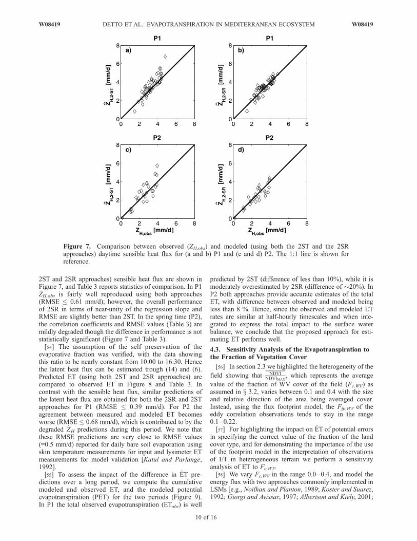
2ST and 2SR approaches) sensible heat flux are shown inFigure 7, and Table 3 reports statistics of comparison. In P1ZH,obs is fairly well reproduced using both approaches(RMSE � 0.61 mm/d); however, the overall performanceof 2SR in terms of near-unity of the regression slope andRMSE are slightly better than 2ST. In the spring time (P2),the correlation coefficients and RMSE values (Table 3) aremildly degraded though the difference in performance is notstatistically significant (Figure 7 and Table 3).[54] The assumption of the self preservation of the

evaporative fraction was verified, with the data showingthis ratio to be nearly constant from 10:00 to 16:30. Hencethe latent heat flux can be estimated trough (14) and (6).Predicted ET (using both 2ST and 2SR approaches) arecompared to observed ET in Figure 8 and Table 3. Incontrast with the sensible heat flux, similar predictions ofthe latent heat flux are obtained for both the 2SR and 2STapproaches for P1 (RMSE � 0.39 mm/d). For P2 theagreement between measured and modeled ET becomesworse (RMSE � 0.68 mm/d), which is contributed to by thedegraded ZH predictions during this period. We note thatthese RMSE predictions are very close to RMSE values(=0.5 mm/d) reported for daily bare soil evaporation usingskin temperature measurements for input and lysimeter ETmeasurements for model validation [Katul and Parlange,1992].[55] To assess the impact of the difference in ET pre-

dictions over a long period, we compute the cumulativemodeled and observed ET, and the modeled potentialevapotranspiration (PET) for the two periods (Figure 9).In P1 the total observed evapotranspiration (ETobs) is well

predicted by 2ST (difference of less than 10%), while it ismoderately overestimated by 2SR (difference of �20%). InP2 both approaches provide accurate estimates of the totalET, with difference between observed and modeled beingless than 8 %. Hence, since the observed and modeled ETrates are similar at half-hourly timescales and when inte-grated to express the total impact to the surface waterbalance, we conclude that the proposed approach for esti-mating ET performs well.

4.3. Sensitivity Analysis of the Evapotranspiration tothe Fraction of Vegetation Cover

[56] In section 2.3 we highlighted the heterogeneity of the

field showing that NDVINDVIMAX

, which represents the average

value of the fraction of WV cover of the field (Fc,WV) asassumed in x 3.2, varies between 0.1 and 0.4 with the sizeand relative direction of the area being averaged cover.Instead, using the flux footprint model, the Ffp,WV of theeddy correlation observations tends to stay in the range0.1–0.22.[57] For highlighting the impact on ET of potential errors

in specifying the correct value of the fraction of the landcover type, and for demonstrating the importance of the useof the footprint model in the interpretation of observationsof ET in heterogeneous terrain we perform a sensitivityanalysis of ET to Fc,WV.[58] We vary Fc,WV in the range 0.0–0.4, and model the

energy flux with two approaches commonly implemented inLSMs [e.g., Noilhan and Planton, 1989; Koster and Suarez,1992; Giorgi and Avissar, 1997; Albertson and Kiely, 2001;

Figure 7. Comparison between observed (ZH,obs) and modeled (using both the 2ST and the 2SRapproaches) daytime sensible heat flux for (a and b) P1 and (c and d) P2. The 1:1 line is shown forreference.

10 of 16


Figure 9. Cumulative observed (ETobs) and modeled (both 2ST and 2SR) ET during (a) P1 and (b) P2.Here the abscissa ‘‘Day’’ represents sequential days excluding precipitation and gaps. The PET isestimated using the Priestley-Taylor equation.

Figure 8. Same as Figure 7, but for evapotranspiration.


11 of 16

W08419

Montaldo and Albertson, 2001]: (1) a two-tile approachwithout the foot print model (2STN) and (2) a lumpedapproach, also without the foot print model (1S). In partic-ular, fluxes are predicted using (1) 2STN, which is equation(6) with a constant value of Ffp,k; since ne = 2 in this case,the constant values of the fraction of land covers are Fc,WV

and 1 � Fc,WV, respectively, and (2) 1S, which is equations(7), (8), (9), and (14) but implemented for the whole system.Hence we estimated lumped values of a, e and c fromliterature values (Table 2), and a mixed value of T s,mix

[=Ts,WV Fc,WV + Ts,NWV (1 � Fc,WV), with Ts,WV and Ts,NWV

the surface temperatures of the WVand NWV, respectively],and use the spatially aggregated BH

�1 estimated previously(see section 4.1) and shown in Figure 6.[59] For the two periods and across the range of Fc,WV,

Figure 10 shows the RMSE of ET and the error of the totalET (eET) defined as

eET ¼ ETT � ETobs;T

ETobs;Tð16Þ

where ETT and ETobs,T are the predicted and observed totalET for the whole period, respectively. For comparison thereference values using the 2ST are also plotted (solid lines).From Figure 10a we note that in P1 the RMSE of 2STNvaries between 0.55 mm/d and 1.21 mm/d, and the RMSEof 1S varies even more, between 0.39 and 1.63, but neverreaching the low value of RMSE of 2ST. The impact on thetotal evapotranspiration is large (Figure 10b) with variationof eLE of more than 200% for both 2STN and 1S across therange of Fc,WV values. Hence ET is significantly sensitive toFc,WV during the P1 characterized by the two highlycontrasting land cover types (bare soil and WV), and

potential errors of Fc,WV can impact the total ET and,consequently, the soil water balance of this water-limitedecosystem.[60] Instead, less sensitivity of ET to Fc,WV is found for P2

(Figures 10c and 10d), because bare soil is not present andsurface thermal states of grasses and WV are more similar(Figure 4).

4.4. Estimates of the B Functions

[61] The daytime b of each land cover component iscomputed across the range of q for both periods(Figure 11). We note the following.[62] 1. The b of WV (bWV) appears insensitive to large

variations in q for both periods, at least when compared tothe soil and grasses. This is not surprising as the typicalshrubs and trees of Mediterranean water-limited ecosystemsare known to be highly tolerant to water content fluctuationsand are usually slower to limit their water losses whencompared to grasses [Larcher, 1995]. For instance, literaturevalues indicate that the Olea can tolerate leaf water poten-tials as extreme as �2 to �3 MPa [Lo Gullo et al., 2003]and �6 MPa [Sakcali and Ozturk, 2004], and the types ofQuercus in these regions can tolerate �2.5 to �6 MPa[Tognetti et al., 1998; Sakcali and Ozturk, 2004] withoutsignificant drop of leaf conductance, while minimal waterpotential values of these resistant shrubs may reach �8 MPa[Larcher, 1995]. These potentials correspond to extremelylow values of q (0.07–0.08), such as estimated by thevan Genuchten’s [1980] soil retention curve using thepedotransfer function of Carsel and Parrish [1988]. Forthis reason, the WV system did not experience excessivesoil moisture stress, and the values of the bWV never fellbelow 0.6 using 2ST or 0.8 using 2SR even for the dry

Figure 10. (a and c) RMSE of ET and (b and d) eET predicted by 2STN and 1S across the range of Fc,WV

for the two periods. For reference the RMSE and eET using the 2ST is also plotted (solid line).

12 of 16


conditions of the summer 2003, which was one of the driestin the last decades in Sardinia.[63] 2. The grass b function (bg) suggests a wilting point

of q � 0.1, and a commencement of transpiration reductionbelow about 0.2. Note that for high q values the bg doesn’treach a value of 1 because other environmental factors (e.g.,temperature, vapor pressure deficit and photosyntheticallyactive radiation may be suboptimal for these grasses) arestressing the plant and increasing the canopy resistance[e.g., Larcher, 1995; Montaldo et al., 2005].[64] 3. During P1 the bare soil b function is close to 0 for

q values below about 0.18, and then increases nonlinearlyfor higher q values as suggested by Parlange et al. [1999],contrasting significantly with bWV.

5. Conclusion

[65] The use of a 2-D footprint model, ground basedthermal infrared observations and high resolution remotesensing images (in conjunction with measurements of windvelocity, air temperature and incoming shortwave and long-wave radiation) provides flux estimates that match well thetower-based observed energy fluxes. For the purposes ofestimating sensible heat flux the use of a proposed two-source random model (2SR), which treats the heat sourcesof WV and NWV separately but computes the bulk heattransfer coefficient as spatially homogeneous, allowsslightly better performance than the use of the commontwo-source tile model (2ST) approach. For implementingthe 2SR approach new relationships between the BH

�1

interfacial transfer coefficient and z0+ are estimated for thetwo composite surfaces (bare soil-WV, and grass-WV) thatcharacterize this Mediterranean ecosystem. The interfacialtransfer coefficient resembles for both composite surfaces abluff-rough surface but with increased momentum rough-ness length. In fact, the dependence of the effective BH

�1 on

z0+ is much stronger (in this case of an open canopy) thanthose reported for either full grass or tree cover.[66] We demonstrated the possibility to estimate accu-

rately ET in heterogeneous ecosystems using surface tem-perature remote observations and high-resolution VIS/NIRremote sensing information. These results are particularlysignificant for remote sensing applications, when landsurface fluxes over a region are estimated from land surfacestates monitored by remote sensing platforms (diagnosticperspective).[67] Moreover, the sensitivity analysis of modeled ET to

the fraction of WV cover (Fc,WV) in this heterogeneousecosystem demonstrates (1) the importance of using afootprint model for interpreting micrometeorological obser-vations and (2) the strong impact of Fc,WV potential errorson the water loss for evapotranspiration and, consequently,on the soil water balance of this water-limited ecosystem inthe summer.[68] Using the proposed approaches we also estimate the

relationships between soil water content and ET for eachland cover component successfully. The typical WV speciesof Sardinia, representative of the broader Mediterraneanwater-limited region, confirm a strong tolerance to pro-longed drought, such as occurred in the summer of 2003(as part of a long-term drought on the island that created awater resources management crisis). Even with the extremedry conditions the WV species were still transpiring at ratesclose to potential. Instead, the grass is less tolerant to watercontent fluctuations, transpires at lower rates than WV, andwilts as the dry summer season commences. The b values ofthe bare soil component are much lower compared to WVand grass b values for dry soil conditions. The switch fromgrass to bare soil has a significant impact on increasing thesensitivity of the bulk ecosystem ET to q during thesummer. Hence we demonstrated that the ET rates of the

Figure 11. Daytime b of each land cover component across the range of q for (a and b) P1 and (c and d)P2 and both the modeling approaches (2ST and 2SR).


13 of 16

W08419

three main landscape components significantly differ forlimiting q values.[69] These results need to be carefully considered in water

resources and land use planning, because land cover changes(i.e., changes of fraction of PFT covers) may impact on thesoil water losses through ET, and therefore on the waterresources availability of these water-limited regions.

Appendix A: Orientation of the EddyCorrelation Sensors in Complex Terrain

[70] In a coordinate system (x, y, z) the three velocitycomponents are defined as u, v and w. Over a sloping planarsurface, the velocity components u and w should be takenparallel and normal to this surface, respectively. If the axisof the sonic anemometer is not orientated parallel to thissurface then part of the horizontal velocity is recorded asvertical velocity (with significant implications to the scalarfluxes). The effective slope varies with topography andhence with the wind direction. Such a slope can beevaluated using a digital elevation model (DEM) map forone direction only or a regression between the horizontalangle co = tan�1 v

u

� �and the vertical angle cv = tan�1 w

u

� �if a

long-term time series is available. The latter approach isadopted here. The relevant flow statistics in the transformedcoordinates can be derived from the original sonic ane-mometer coordinate (shown in capital letters for clarity)system using:means:

u ¼ A1A3U þ A2A3V þ A4W

v ¼ 0

w ¼ �A1A4U � A2A4V þ A3W

ðA1Þ

variances:

u02 ¼ A23 A2

1U02 þ A2

2V02 þ 2A1A2U 0V 0

� �þ A2

4W02 þ 2A3A4

� A1W 0U 0 þ A2W 0V 0� �

v02 ¼ A21V

02 þ A22U

02 þ 2A1A2U 0W 0 ðA2Þ

w02 ¼ A24 A2

1U02 þ A2

2V02

� �þ A2

3W02 � 2A3A4

� A1W 0U 0 þ A2W 0V 0 þ A1A2U 0V 0� �

stresses:

u0v0 ¼ A21 � A2

2

� �A3U 0V 0 � A1A2U 02 þ A1A2A3V 02 þ A1A4W 0V 0

� A2A4W 0U 0

u0w0 ¼ A1A23 � A1A

24

� �U 0W 0 � A2

1A3A4U 02 � 2A1A2A3A4U 0V 0

þ A2A23 � A2A

24

� �W 0V 0 � A2

2A3A4V 02 þ A3A4W 02

u0v0 ¼ A21 � A2

2

� �A3U 0V 0 � A1A2U 02 þ A1A2A3v0

2 þ A1A4W 0V 0

� A2A4W 0U 0

ðA3Þ

scalar fluxes, F:

w0F0 ¼ A3W 0F0 � A1A4U 0F0 � A2A4V 0F0 ðA4Þ

where A1 = cosco, A2 = sinco, A3 = coscv, A4 = sincv. In themanuscript, we used small-case letters as already trans-formed variables for consistency with the literature.

Appendix B: Extension of the H2000 FootprintModel of Hsieh et al. [2000] to Two Dimensions

[71] The basic equation of the H2000 model and itsextension to 2-D are discussed here. The cross-wind inte-grated footprint

Fy ¼ 1

k2v x2DzPu Lj j1�P

e

DzPu Lj j1�P

k2v x ðB1Þ

where zu is the length scale of H2000, L is the Obukhov’slength [Brutsaert, 1982], kv (=0.4) is the von Karman’sconstant, D and P are similarity constants which valueschange for unstable, neutral and stable atmosphericconditions [Hsieh et al., 2000].[72] Because this model predicts only the cross-wind

integrated footprint, the contribution of lateral dispersionmust be added to generate a 2-D source area function.Starting from the assumption that diffusion in the verticaland crosswind direction can be treated independently, f canbe estimated through

f x; y; zmð Þ ¼ Dy x; yð ÞFy x; zmð Þ ðB2Þ

whereDy is the lateral diffusion and is commonly assumed tobe Gaussian [Schmid, 1994], so that it can be estimated as:

Dy x; yð Þ ¼ 1ffiffiffiffiffiffi2p

psy

e�1

2y

sy

� �2

ðB3Þ

where the standard deviation sy can be related to the standarddeviation in the lateral wind fluctuations, sv as [Eckman,1994]:

sy ¼ a1zomsvu�

x

zom

� �p1

ðB4Þ

where u* is the friction velocity, zom is the roughness lengthfor momentum, and a1 (=0.3) and p1 (=0.86) are similarityparameters.

[73] Acknowledgments. The participation of M. Detto, M. Mancini,and N. Montaldo in this research was supported by the Ministero dell’U-niversita e della Ricerca Scientifica e tecnologica of Italy through grant2002084552_003 and the Istituto Nazionale della montagna (Agenzia2002). The participation of J. D. Albertson and G. Katul in this researchwas supported by the Office of Science (BER), U.S. Department of Energy(grants DE-FG02-00ER63015 and DE-FC02-03ER63613) and the NationalScience Foundation (NSF-EAR 0208258). We thank Paolo Botti, MariaAntonietta Dessena, and Gianni Borghero of the Ente Autonomo delFlumendosa (Cagliari, Italy) for the support in the tower setup andmaintenance. Finally, we thank the three anonymous reviewers and NelsonDias for their useful comments.

ReferencesAlbertson, J. D., and G. Kiely (2001), On the structure of soil moisture timeseries in the context of land surface models, J. Hydrol., 243(1–2), 101–119.

Albertson, J. D., and N. Montaldo (2003), Temporal dynamics of soilmoisture variability: 1. Theoretical basis, Water Resour. Res., 39(10),1274, doi:10.1029/2002WR001616.

14 of 16


Altese, E., O. Bolognani, M. Mancini, and P. A. Troch (1996), Retrievingsoil moisture over bare soil from ERS-1 synthetic aperture radar data:Sensitivity analysis based on a theoretical surface scattering model andfield data, Water Resour. Res., 32(3), 653–661.

Baldocchi, D., and S. Rao (1995), Intra-field variability of scalar fluxdensities across a transition between a desert and an irrigated potato site,Boundary Layer Meteorol., 76, 109–136.

Baldocchi, D., J. Finnigan, K. Wilson, K. T. U. Paw, and E. Falge (2000),On measuring net ecosystem carbon exchange over tall vegetation oncomplex terrain, Boundary Layer Meteorol., 96(1–2), 257–291.

Baldocchi, D. D., L. Xu, and N. Kiang (2004), How plant functional-type,weather, seasonal drought, and soil physical properties alter water andenergy fluxes of an oak-grass savanna and an annual grassland, Agric.Forest. Meteorol., 123, 13–39.

Blanken, P. D., T. A. Black, P. C. Yang, H. H. Neumann, Z. Nesic,R. Staebler, G. den Hartog, M. D. Novak, and X. Lee (1997), Energybalance and canopy conductance of a boreal aspen forest: Partitioningoverstory and understory components, J. Geophys. Res., 102(D24),28,915–28,927.

Brunetti, M., M. Maugeri, T. Nanni, and A. Navarra (2002), Droughts andextreme events in regional daily Italian precipitation series, Int. J. Cli-matol., 22, 543–558.

Brutsaert, W. (1982), Evaporation Into the Atmosphere, 299 pp., Springer,New York.

Brutsaert, W. (2005), Hydrology: An Introduction, 605 pp., CambridgeUniv. Press, New York.

Bugbee, B., M. Droter, O. Monje, and B. Tanner (1998), Evaluation andmodification of commercial infra-red transducers for leaf temperaturemeasurement, Adv. Space Res., 22(10), 1425–1434.

Caparrini, F., F. Castelli, and D. Entekhabi (2004), Estimation of surfaceturbulent fluxes through assimilation of radiometric surface temperaturesequences, J. Hydrometeorol., 5(1), 145–159.

Carlson, T. N., and D. A. Ripley (1997), On the relation between NDVI,fractional vegetation cover, and leaf area index, Remote Sens. Environ.,62(3), 241–252.

Carsel, R. F., and R. S. Parrish (1988), Developing joint probability dis-tributions of soil water retention characteristics, Water Resour. Res.,24(5), 755–769.

Ceballos, A., J. Martinez-Fernandez, and M. A. Luengo-Ugidos (2004),Analysis of rainfall trends and dry periods on a pluviometric gradientrepresentative of Mediterranean climate in the Duero Basin, Spain, J. AridEnviron., 58(2), 215–233.

Crago, R., and W. Brutsaert (1996), Daytime evaporation and the self-preservation of the evaporative fraction and the Bowen ratio, J. Hydrol.,178(1–4), 241–255.

Dash, P., F. M. Gottsche, F. S. Olesen, and H. Fischer (2002), Land surfacetemperature and emissivity estimation from passive sensor data: Theoryand practice-current trends, Int. J. Remote Sens., 23(13), 2563–2594.

Eckman, R. M. (1994), Re-examination of empirically derived formulas forhorizontal diffusion from surface sources, Atmos. Environ., 28(2), 265–272.

Entekhabi, D., I. Rodriguez-Iturbe, and F. Castelli (1996), Mutual interac-tion of soil moisture state and atmospheric processes, J. Hydrol., 184, 3–17.

Entekhabi, D., et al. (2004), The hydrosphere state (Hydros) satellite mis-sion: An Earth system pathfinder for global mapping of soil moisture andland freeze/thaw, IEEE Trans. Geosci. Remote Sens., 42(10), 2184–2195.

Fernandez, J. B. G., M. R. G. Mora, and F. G. Novo (2004), Vegetationdynamics of Mediterranean shrublands in former cultural landscape atGrazalema Mountains, south Spain, Plant Ecol., 172(1), 83–94.

Finnigan, J. (2004), The footprint concept in complex terrain, Agric. For.Meteorol., 127(3–4), 117–129.

Gamon, J. A., C. B. Field, M. L. Goulden, K. L. Griffin, A. E. Hartley, J. G.Penuelas, and R. Valentini (1995), Relationships between NDVI, canopystructure, and photosynthesis in 3 Californian vegetation types, Ecol.Appl., 5(1), 28–41.

Garratt, J. R. (1992), The Atmospheric Boundary Layer, Cambridge Univ.Press, New York.

Giorgi, F., and R. Avissar (1997), Representation of heterogeneity effects inearth system modeling: Experience from land surface modeling, Rev.Geophys., 35(4), 413–438.

Gutman, G., and A. Ignatov (1997), The derivation of the green vegetationfraction from NOAA/AVHRR data for use in numerical weather predic-tion models, Int. J. Remote Sens., 19(8), 1533–1543.

Halldin, S., S.-E. Gryningb, L. Gottschalkc, A. Jochumd, L.-C. Lundina,and A. A. Van de Griend (1999), Energy, water and carbon exchange in a

boreal forest landscape—NOPEX experiences, Agric. For. Meteorol.,98(9), 5–29.

Holah, N., N. Baghdadi, M. Zribi, A. Bruand, and C. King (2005),Potential of ASAR/ENVISAT for the characterization of soil surfaceparameters over bare agricultural fields, Remote Sens. Environ., 96(1),78–86.

Hsieh, C. I., G. Katul, and T. Chi (2000), An approximate analytical modelfor footprint estimation of scalar fluxes in thermally stratified atmo-spheric flows, Adv. Water Resour., 23(7), 765–772.

Jackson, R. B., J. L. Banner, E. G. Jobbagy, W. T. Pockman, and D. H. Wall(2002), Ecosystem carbon loss with woody plant invasion of grasslands,Nature, 418, 623–626.

Jackson, T. J. (1997a), Soil moisture estimation using special satellite mi-crowave/imager satellite data over a grassland region, Water Resour.Res., 33(6), 1475–1484.

Jackson, T. (1997b), Experiment plan: Southern Great Plains 1997 (SGP97)Hydrology Experiment, report, Hydrol. Lab., Agric. Res. Serv., Belts-ville, Md.

Katul, G. G., and M. B. Parlange (1992), Estimation of bare soil eva-poration using skin temperature measurements, J. Hydrol., 132, 91–106.

Kljun, N., P. Calanca, M. W. Rotachhi, and H. P. Schmid (2004), A simpleparameterisation for flux footprint predictions, Boundary LayerMeteorol., 112(3), 503–523.

Koster, R. D., and M. J. Suarez (1992), Modeling the land surface boundaryin climate models as a composite of independent vegetation stands,J. Geophys. Res., 97(D3), 2697–2715.

Kurc, S. A., and E. E. Small (2004), Dynamics of evapotranspiration insemiarid grassland and shrubland ecosystems during the summer mon-soon season, central New Mexico, Water Resour. Res., 40, W09305,doi:10.1029/2004WR003068.

Kustas, W. P., and J. M. Norman (1999), Evaluation of soil and vegetationheat flux predictions using a simple two-source model with radiometrictemperatures for partial canopy cover, Agric. For. Meteorol., 94(1), 13–29.

Kustas, W. P., J. H. Prueger, and L. E. Hipps (2002), Impact of usingdifferent time-averaged inputs for estimating sensible heat flux of ripar-ian vegetation using radiometric surface temperature, J. Appl. Meteorol.,41(3), 319–332.

Kustas, W. P., J. M. Norman, M. C. Anderson, and A. N. French (2003),Estimating subpixel surface temperatures and energy fluxes from thevegetation index-radiometric temperature relationship, Remote Sens. En-viron., 85(4), 429–440.

Larcher, W. (1995), Physiological Plant Ecology, Springer, New York.Lelieveld, J., et al. (2002), Global air pollution crossroads over the Medi-terranean, Science, 298(5594), 794–799.

Lo Gullo, M. A., S. Salleo, R. Rosso, and P. Trifilo (2003), Droughtresistance of 2-year-old saplings of Mediterranean forest trees in thefield: Relations between water relations, hydraulics and productivity,Plant Soil, 250(2), 259–272.

Mancini, M., R. Hoeben, and P. A. Troch (1999), Multifrequency radarobservations of bare surface soil moisture content: A laboratory experi-ment, Water Resour. Res., 35(6), 1827–1838.

Maselli, F., M. Chiesi, and M. Bindi (2004), Multi-year simulation ofMediterranean forest transpiration by the integration of NOAA-AVHRRand ancillary data, Int. J. Remote Sens., 25(19), 3929–3941.

Massman, W. J. (1999), A model study of kB(H)(�1) for vegetated surfacesusing ‘‘localized near-field’’ Lagrangian theory, J. Hydrol., 223(1–2),27–43.

Montaldo, N., and J. D. Albertson (2001), On the use of the force-restoreSVAT model formulation for stratified soils, J. Hydrometeorol., 2(6),571–578.

Montaldo, N., J. D. Albertson, M. Mancini, and G. Kiely (2001), Robustsimulation of root zone soil moisture with assimilation of surface soilmoisture data, Water Resour. Res., 37(12), 2889–2900.

Montaldo, N., V. Toninelli, J. D. Albertson, M. Mancini, and P. A. Troch(2003), The effect of background hydrometeorological conditions on thesensitivity of evapotranspiration to model parameters: Analysis withmeasurements from an Italian alpine catchment, Hydrol. Earth Syst.Sci., 7(6), 848–861.

Montaldo, N., R. Rondena, J. D. Albertson, and M. Mancini (2005), Parsi-monious modeling of vegetation dynamics for ecohydrologic studies ofwater-limited ecosystems, Water Resour. Res., 41, W10416,doi:10.1029/2005WR004094.

Moonen, A. C., L. Ercoli, M. Mariotti, and A. Masoni (2002), Climatechange in Italy indicated by agrometeorological indices over 122 years,Agric. For. Meteorol., 111(1), 13–27.


15 of 16

W08419

Mouillot, F., S. Rambal, and R. Joffre (2002), Simulating climate changeimpacts on fire frequency and vegetation dynamics in a Mediterranean-type ecosystem, Global Change Biol., 8(5), 423–437.

Noilhan, J., and S. Planton (1989), A simple parameterization of land sur-face processes for meteorological models,Mon. Weather Rev., 117, 536–549.

Parlange, M. B., J. D. Albertson, W. E. Eichinger, A. T. Cahill, and T. J.Jackson (1999), Evaporation: Use of fast response turbulence sensors,Raman lidar and passive microwave remote sensing, in Vadose ZoneHydrology: Cutting Across Disciplines, edited by M. B. Parlange andJ. W. Hopmans, pp. 260–278, Oxford Univ. Press, New York.

Ragab, R., D. Moidinis, J. Albergel, J. Khouri, A. Drubi, and S. Nasri(2001), The HYDROMED model and its application to semi-arid Med-iterranean catchments with hill reservoirs: 2. Rainfall-runoff model ap-plications to three Mediterranean hill reservoirs, Hydrol. Earth Syst. Sci.,5(4), 554–562.

Ramirez-Sanz, L., M. A. Casado, J. M. de Miguel, I. Castro, M. Costa, andF. D. Pineda (2000), Floristic relationship between scrubland and grass-land patches in the Mediterranean landscape of the Iberian Peninsula,Plant Ecol., 149(1), 63–70.

Reichle, R. H., R. D. Koster, J. R. Dong, and A. A. Berg (2004), Global soilmoisture from satellite observations, land surface models, and grounddata: Implications for data assimilation, J. Hydrometeorol., 5(3), 430–442.

Reynolds, J., P. Kemp, and J. Tenhunen (2000), Effects of long-term rainfallvariability on evapotranspiration and soil water distribution in the Chi-huan desert: A modeling analysis, Plant Ecol., 150, 145–159.

Richards, J. A. (1999), Remote Sensing Digital Image Analysis, Springer,New York.

Rodriguez-Iturbe, I. (2000), Ecohydrology: A hydrologic perspective ofclimate-soil-vegetation dynamics, Water Resour. Res., 36(1), 3–9.

Sakcali, M. S., and M. Ozturk (2004), Eco-physiological behaviour of somemediterranean plants ad suitable candidates of degraded areas, J. AridEnviron., 57(2), 141–153.

Scanlon, T. M., J. D. Albertson, K. K. Caylor, and C. A. Williams (2002),Determining land surface fractional cover from NDVI and rainfall timeseries for a savanna ecosystem, Remote Sens. Environ., 82(2–3), 376–388.

Schmid, H. P. (1994), Source areas for scalars and scalar fluxes, BoundaryLayer Meteorol., 67(3), 293–318.

Schmid, H. P. (1997), Experimental design for flux measurements: Match-ing scales of observations and fluxes, Agric. For. Meteorol., 87, 179–200.

Schmid, H. P. (2002), Footprint modelling for vegetation atmosphere ex-change studies: A review and perspective, Agric. For. Meteorol., 113,159–183.

Scholes, R. J., and S. R. Archer (1997), Tree-grass interactions in savannas,Annu. Rev. Ecol. Syst., 28, 517–544.

Shimabukuro, Y. E., V. C. Carvalho, and B. F. T. Rudorff (1997), NOAA-AVHRR data processing for the mapping of vegetation cover, Int. J.Remote Sens., 18(3), 671–677.

Sophocleous, M. (2000), From safe yield to sustainable development ofwater resources—The Kansas experience, J. Hydrol., 235(1–2), 27–43.

Su, Y., P. S. Huang, C. F. Lin, and T. M. Tu (2004), Approach to maximizeincreased details and minimize color distortion for IKONOS and Quick-Bird image fusion, Opt. Eng., 43(12), 3029–3037.

Tognetti, R., A. Longobucco, F. Miglietta, and A. Raschi (1998), Transpira-tion and stomatal behaviour of Quercus ilex plants during the summer ina Mediterranean carbon dioxide spring, Plant Cell Environ., 21(6), 613–622.

Twine, T. E., W. P. Kustas, J. M. Norman, D. R. Cook, P. R. Houser, T. P.Meyers, J. H. Prueger, P. J. Starks, and M. L. Wesely (2000), Correctingeddy-covariance flux underestimates over a grassland, Agric. For. Me-teorol., 103(3), 279–300.

van Genuchten, M. T. (1980), A closed-form equation for predicting thehydraulic conductivity of unsaturated soils, Soil Sci. Soc. Am. J., 44(5),892–898.

Ventura, F., P. R. Pisa, and E. Ardizzoni (2002), Temperature and precipita-tion trends in Bologna (Italy) from 1952 to 1999, Atmos. Res., 61(3),203–214.

Verhoef, A., H. A. R. DeBruin, and B. VandenHurk (1997), Some practicalnotes on the parameter kB(�1) for sparse vegetation, J. Appl. Meteorol.,36(5), 560–572.

Vermote, E. F., D. Tanre, J. L. Deuze, M. Herman, and J. J. Morcrette(1997), Second simulation of the satellite signal in the solar spectrum,6S: An overview, IEEE Trans. Geosci. Remote, 35(3), 675–686.

Vesala, T., U. Rannik, M. Leclerc, T. Foken, and K. Sabelfeld (2004), Fluxand concentration footprints, Agric. For. Meteorol., 127(3–4), 111–116.

Webb, E. K., G. I. Pearman, and R. Leuning (1980), Correction of fluxmeasurements for density effects due to heat and water-vapor transfer, Q.J. R. Meteorol. Soc., 106(447), 85–100.

Western, A. W., R. B. Grayson, and G. Bloschl (2002), Scaling of soilmoisture: A hydrologic perspective, Annu. Rev. Earth Planet. Sci., 30,149–180.

Williams, C. A., and J. D. Albertson (2004), Soil moisture controls oncanopy-scale water and carbon fluxes in an African savanna, WaterResour. Res., 40, W09302, doi:10.1029/2004WR003208.

��J. D. Albertson and G. Katul, Department of Civil and Environmental

Engineering, Pratt School of Engineering, Duke University, Durham, NC27708, USA.

M. Detto, M. Mancini, and N. Montaldo, DIIAR, Fantoli LaboratoryBuilding, Politecnico di Milano, Piazza Leonardo da Vinci, 32, I-20133Milano, Italy. ([email protected])

16 of 16


click here full article soil moisture and vegetation ... · soil moisture and vegetation controls...

Documents