clever clean vehicles research: lca and policy measures wp2 lca report.… · oil and natural gas...
TRANSCRIPT

`
Clean Vehicles Research: LCA and Policy Measures
Boureima Fayçal
Prof. Dr. ir. Van Mierlo Joeri
Vrije Universiteit Brussel
Department of Electrical Engineering and Energy Technology (ETEC)
Mobility and automotive technology research group (MOBI)
CLEVER Clean Vehicles Research: LCA and Policy Measures
LCA report
Boureima Fayçal-Siddikou
Wynen Vincent
Sergeant Nele
Rombaut Heijke
Messagie Maarten
Prof. Dr. ir. Van Mierlo Joeri
Vrije Universiteit Brussel
Department of Electrical Engineering and Energy Technology (ETEC)
Mobility and automotive technology research group (MOBI)
`
Clean Vehicles Research: LCA and Policy Measures
Department of Electrical Engineering and Energy Technology (ETEC)
2
Table of contents
LCA report ............................................................................................................................. 1
Table of contents .................................................................................................................... 2
Table of tables ........................................................................................................................ 3
ACRONYMS, ABBREVIATIONS AND UNITS ................................................................. 6
Introduction ........................................................................................................................... 8
I. Goal of the study ................................................................................................................. 9
II. Scope of the study ............................................................................................................. 9
II.1 Functional unit ................................................................................................................ 9
II.2 Data quality requirements ............................................................................................. 11
II.3 Data uncertainties ......................................................................................................... 19
III. The CLEVER LCA tool ................................................................................................ 20
III.1 Range based modelling system .................................................................................... 20
III.2 Vehicle fleet segmentation .......................................................................................... 21
IV. Inventory and data Collection ....................................................................................... 22
IV.1. Manufacturing ............................................................................................................ 22
IV.2. Fuel Cell Electric Vehicles (FCEV) ............................................................................ 23
IV.3. Exhaust after treatment systems ................................................................................. 24
IV.4. Electricity .................................................................................................................. 25
IV.5. The Electrabel electricity mix (main Belgian electricity provider) .............................. 26
IV.6. Oil and Natural gas .................................................................................................... 26
IV.7. Hydrogen ................................................................................................................... 28
IV.8. Diesel and Petrol ........................................................................................................ 30
IV.9. LPG (Liquefied Petroleum Gas) ................................................................................. 32
IV.10. CNG (Compressed Natural Gas) .............................................................................. 33
IV.11. Bio-fuels .................................................................................................................. 34
IV.12. Battery Ellectric Vehicles, Fuel Cell Electric Vehicle and Hybrid Electric Vehicles . 40
IV.13. Maintenance ............................................................................................................. 41
IV.14. End-of-life ............................................................................................................... 41
IV.15. Tank to Wheel (TTW) data....................................................................................... 43
IV.16 Conclusion ................................................................................................................ 47
V. Life Cycle Impact Assessment ........................................................................................ 47
VI. The RangeLCA software ............................................................................................... 51
VII. Results and discussion .................................................................................................. 52
VIII. Scientific validation of the Ecoscore approach .......................................................... 56
VIII.1 Introduction .............................................................................................................. 56
VIII.2 Ecoscore methodology.............................................................................................. 57
VIII.2 Vehicle selection ...................................................................................................... 58
VIII.3 Comparison of Total Impact (Ecoscore) and LCA results ......................................... 59
IX. Optimal time for replacement ....................................................................................... 63
IX.1 Introduction ................................................................................................................ 63
IX.2 Methodology ............................................................................................................... 63
IX.3 Inventory..................................................................................................................... 64
IX.4 Results ........................................................................................................................ 66
X. Applicability of the methodology for other transport modes ........................................ 75
XI. Main conclusions of the LCA ........................................................................................ 76
References ............................................................................................................................ 80

3
Table of tables
Table 1: Datasets used to model the bodyshell of the different vehicles and the fuel
production ............................................................................................................. 13
Table 2: Datasets used to model the manufacturing of the assumed fuel cell ................. 14
Table 3: Datasets used to model the manufacturing of the NiCd battery ........................ 14
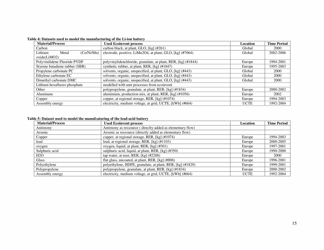
Table 4: Datasets used to model the manufacturing of the Li-ion battery ...................... 15
Table 5: Dataset used to model the manufcaturing of the lead-acid battery ................... 15
Table 6: Datasets used to model the manufacturing of the NiMH battery ....................... 16
Table 7: Datasets used model the manufacturing of the hydrogen tank ......................... 16
Table 8: Datasets used to model the hydrometallurgical recycling process of the Li-ion
battery ................................................................................................................. 17
Table 9: Datasets used to model the pyrometallurgical recycling process of the NiMH
battery ................................................................................................................. 17
Table 10: Datasets used to model the campine recycling process of lead-acid battery ..... 17
Table 11: Datasets used to model the pyrometallurgical recycling process of NiCd battery
............................................................................................................................ 18
Table 12: basic uncertainty factors .......................................................................... 19
Table 13: Default uncertainty factors applied with the pedigreed matrix ....................... 20
Table 14: Vehicle segmentation in Belgium ................................................................ 21
Table 15: Manufacturing data of the theoretical vehicle .............................................. 22
Table 16: Manufacturing data of the assumed fuel cell [27, 28] ................................... 23
Table 17: Manufacturing data of the assumed hydrogen tank [27, 28] .......................... 23
Table 18: Needed resources for the Manufacturing of 1 kg of carbon fibre [29] .............. 24
Table 19: Manufacturing data of a sedan-specific catalytic converter exhaust system .... 24
Table 20: After treatment efficiency of the catalytic converter ..................................... 25
Table 21: Belgian electricity supply mix: of 1 kWh ..................................................... 25
Table 22: Emissions induced by the production and the distribution of 1 Electrabel kWh []
............................................................................................................................ 26
Table 23: Belgian oil suppliers in 2007 [34] ............................................................... 27
Table 24: Belgium natural gas suppliers in 2007 ....................................................... 27
Table 25: Main input for the onshore production of 1 Nm3 of natural gas in the Netherlands
............................................................................................................................ 27
Table 26: Main input for the offshore production of 1 Nm3 of natural gas in Norway [35]. 27
Table 27: Main inputs for the onshore production of 1 Nm3 of natural gas in Algeria [35]. 28
Table 28: Main inputs for the onshore production of 1 Nm3 of natural gas in Russia [35]. 28
Table 29: WTT data of SMR hydrogen including the hydrogen production and the
compression [36] ................................................................................................... 29
Table 30: Needed resources to produce 1 kg of liquid hydrogen via fossil fuel cracking
process ................................................................................................................ 30
Table 31: Main input of the production of 1 kg of normal diesel [38]. ............................ 31
Table 32: Main input for the production of 1 kg unleaded petrol [38]. ........................... 32

4
Table 33: Main input for the production of 1 kg of propane/butane [38]. ....................... 33
Table 34: Energy consumption during the liquefaction and the distribution of 1 GJ of LPG
[40]. .................................................................................................................... 33
Table 35: Main input for the production of 1liter of LPG [38, 40]. ................................. 33
Table 36: Main input for the production of 1 kg of rye ethanol [43]. ............................. 35
Table 37: Ship transport of 1 kg of sugar cane ethanol from Brazil to Europe [43]. ........ 35
Table 38: Main inputs for the production of 1 kg of sugar cane ethanol [43]. ................. 35
Table 39: Main inputs for the production of 1 kg of sugar beet ethanol [43] .................. 36
Table 40: Main inputs for the production of 1 kg of grass ethanol [43] .......................... 36
Table 41: Main inputs for the production of 1 kg of wood ethanol [43] .......................... 37
Table 42: Main input for the production of 1 kg of synthetic gas from wood [43]. ........... 37
Table 43: Main input for the production of 1 kg of methanol from synthetic gas [43]. ..... 38
Table 44: Main input for the extraction of 1 kg of rape oil [43]..................................... 38
Table 45: Main inputs for the production of 1 kg of rape methyl ester [43]. ................... 38
Table 46: Main inputs for the extraction of 1 kg of soybean oil [43]. ............................. 39
Table 47: Main inputs for the production of 1 kg of soybean methyl ester [43] .............. 39
Table 48: Main input for the production of 1 kg of waste cooking oil methyl ester [43]. .. 39
Table 49: Energy consumption for the production of 1Nm3 of biogas from biowaste [43]. 40
Table 50: Theoretical maintenance process. [47, 48]. ................................................. 41
Table 51: Non-exhaust emissions of passenger vehicle [49] ........................................ 41
Table 52: Material breakdown of a tire [47, 48] ......................................................... 41
Table 53: Main inputs for the production of 1 kg of lubricant oil [38]. ........................... 41
Table 54: Recovery rates of end-of -life vehicle materials [10]. .................................... 42
Table 55: Hydrometallurgical recycling of Lithium Ion battery [51] ............................... 42
Table 56: Pyrometallurgical recycling of NiMH battery [51] .......................................... 43
Table 57: Campine Lead acid battery recycling [51] ................................................... 43
Table 58: Pyrometallurgical recycling of NiCd battery [51]........................................... 43
Table 59: heavy metal emissions of passenger car [49] .............................................. 45
Table 60: TTW emissions of bio-fuel vehicles [43]. ..................................................... 46
Table 61: TTW emissions of the Citroen C4 using different blends of diesel. ................... 46
Table 62: TTW emissioons of the Saab 9.5 BioPower using different blends of petrol [53] 46
Table 63: TTW emissions of the Volvo F50 using different blends of petrol [53] .............. 46
Table 64: TTW emissions of 2 prototype hydrogen vehicles ......................................... 47
Table 65: Pre-selection of characterisation models for further analysis [60] ................... 48
Table 66: IPCC 2007 (100a) including biogenic CO2 and CO2 uptake from the air [61] .... 49
Table 67: CML 2001 Air acidification [62] .................................................................. 50
Table 68: CML 2001 eutrophication [62] ................................................................... 50
Table 69: Non renewable energy (BUWAL/RDC) ......................................................... 50
Table 70: Renewable energy (BUWAL/RDC) ............................................................... 51

5
Table 71: Impact 2002+ respiratory inorganics (endpoints) [64] .................................. 51
Table 72: Eco-indicator 99 Hieratchist, Resources, Mineral extraction damage (midpoints)
[63] ..................................................................................................................... 51
Table 73: Selected vehicles with their fuel consumption, emissions, Ecoscore and Total
Impact (TI). .......................................................................................................... 58
Table 74: Overview of the tailpipe emissions, fuel consumption and weight. .................. 65
Table 75: Overview of total life cycle impact of the considered vehicle technologies ........ 66
Table 76: Overview of the different environmental impacts of the manufacturing phase .. 69
Table 77: Overview of the different environmental impacts of the use phase ................. 69
Table 78: Overview of the different environmental impacts of the End-of-Life treatment . 69
Table 79: Environmental breakeven point for the greenhouse effect when replacing a
vehicle in column i with vehicle in row j .................................................................... 71
Table 80: Environmental breakeven point for acidification when replacing a vehicle in
column i with vehicle in row j ................................................................................... 72
Table 81: Environmental breakeven point for eutrophication when replacing a vehicle in
column i with vehicle in row j ................................................................................... 72
Table 82: Environmental breakeven point for energy when replacing a vehicle in column i
with vehicle in row j ............................................................................................... 72
Table 83: Environmental breakeven point for respiratory effects when replacing a vehicle in
column i with vehicle in row j ................................................................................... 73
Table 84: Environmental breakeven point for mineral extraction damage when replacing a
vehicle in column i with vehicle in row j .................................................................... 73

6
ACRONYMS, ABBREVIATIONS AND UNITS ABS Acrylonitrile Butadiene Styrene
Ag Silver
Al2O3 Aluminum Oxide
BEV Battery Electric Vehicle
BIOSES BIOfuel Sustainable End uSe
BTL Biomass-to-Liquid
CaCl2 Calcium Chloride
CeO2 Cerium Oxide
Cd Cadmium
CHCL3 Trichloromethane
CLEVER Clean Vehicle Research: LCA and Policy Measures
CNG Compressed natural Gas
CRT Continuously Regenerated Trap
Cu O Copper Onoxide
DfE Design for Environment
ECE (UDC) Urban Driving Cycle
EoL End-of-Life
ETBE Ethyl Tert-Butyl Ether
ETEC Department of Electrotechnical Engineering and Energy Technology
EuroNcap: European New Car Assessment Program
FCAI: Federal Chamber of Automotive Industry of Australia
FCEV Fuel Cell Engine Vehicle
FISITA: International Federation of Automotive Engineering Societies
GJ Giga Joule
HCl Hydrogen Choride
HEV Hybrid Electric Vehicle
HF Hydrogen Fluoride
n.a not available
NH3 Ammonia
HNO3 Nitric acid
kg kilogram
ICEV Internal Combustion Engine Vehicle
LCA Life Cycle Assessment
LCI Life Cycle Inventory
Li-ion Lithium-ion

7
LPG Liquefied Petroleum Gas
LTDD Life Time Driven Distance
m meter
Mo Molybdenum
MTBE Methyl Tert-Butyl Ether
NEDC New European Driving Cycle
NG Natural Gas
NiMH Nickel Metal Hydride
NiCd Nickel Cadmium
Nm3 Normal cubic meter
O2 Oxygen
OVAM Openbare Vlaamse Afvalstoffen Maatschappij – Public Flemish Waste Company
Pb Lead
PGM Platinum Group Metals
PM Particulate Mater
ppm parts per million
PVDF Polyvinilidene Fluoride
RDC Research, Development and Consulting
RME Rape Methyl Ester
SCR Selective Catalytic Reduction
SBR Styrene Butadiene Rubber
SME Soybean Methyl Ester
SMR Steam reforming
SUV Sports Utility Vehicle
SUBAT SUStainable BATtery
tkm ton-kilometer
TiO2 Titanium Dioxide
TTW Tank-to-Wheel
UCTE Union for the co-ordination of transmission of electricity
VSP Vehicle Simulation Program
VUB Vrije Universiteit Brussel
WTT Well-to-Tank
WTW Well-to-Wheel
Zn Zinc
ZrO2 Zirconium Oxide

8
Introduction The CLEVER project aims at fulfilling the following objectives:
• Create an objective image of the environmental impact of vehicles with conventional
and alternative fuels and/or drive trains;
• Investigate which price instruments and other policy measures are possible to realize a
sustainable vehicle choice;
• Examine the external costs and verify which barriers exist for the introduction of clean
vehicle technologies on the Belgian market;
• Analyse the global environmental performances of the Belgian car fleet;
• Formulate recommendations for the Belgian government to stimulate the purchase and
use of clean vehicles
For the environmental part of the CLEVER project, an LCA methodology has been used. To
perform the LCA, an input and output data gathering process called Life Cycle Inventory (LCI)
has been done. The LCI step provides information on all the inputs and outputs from and to the
environment from all the unit processes involved in the product system with respect to the
functional unit which is a lifetime driven distance of 230,500 km. In other words, the life cycle
inventory is the compilation of all the needed materials, chemicals, energies and all the
emissions related to the fulfillment of the functional unit. In the CLEVER project, a special data
gathering strategy has been developed and executed for that issue. A literature review has been
performed and a list of all the relevant European and Belgian projects (CONCAWE [1],
ExternE [2], Libiofuels [3], PREMIA [4], SGS-INGENIEURE [5], SenterNovem [6], Camden
LCA [7], VITO & 3E [8]…) was established. All the relevant data from those projects were
analysed and centralized in a specific data gathering template.
When specific Belgian data are not available, average European data are considered.
As the CLEVER project aims at developing a per-model applicable LCA, the Belgian fleet has
been classified into nine different categories (see chapter I). This categorization has enabled to
adapt the Tank-to-Wheel emissions from the Ecoscore database to the different Belgian market
segments. For the other life cycle phases, the Ecoinvent database has been used to calculate LCI
of materials, manufacturing processes, energy production, fuel production and distribution for
both conventional and alternative vehicles. Detailed LCI data of different battery technologies
for hybrid electric (HEV) and battery electric vehicles (BEV) have been collected from the
SUBAT project [9]. The use of supercapacitors in HEV has been included as well. Thanks to
the OVAM study on the vehicles’ end-of-life in Belgium, all the recycling and energy recovery

9
rates per material with respect to the real efficiency of Belgian recycling plants were collected
[10]..
Notice: For reminding the Ecoinvent Data v2.01 [11] is the reference LCI database of the
CLEVER project. It contains about 4000 datasets of products and services covering energy,
transport, building materials, wood, chemicals, electronics, mechanical engineering, paper and
pulp, plastics, renewable fibers, metals, waste treatment and agricultural products. Each dataset
contains all the resources and all the emissions (towards soil, air and water) linked to the
production of the corresponding product or service. Thereby it is important to keep in mind that
the information contained in all the tables of this report is just summarizing the main inputs
(materials, energy and chemicals) for the production of the corresponding products or services.
Unit processes, such as waste treatment, transport, industrial plants, etc. are taken into account
even if they don’t appear explicitly in the tables (for convenience reasons). The complete
Ecoinvent datasets have been checked and are used in the CLEVER LCA model.
I. Goal of the study The Clever LCA study has been commissioned by the Belgian Science Policy (BELSPO) and
its intended purpose is to perform a comparative assessment of different vehicles (conventional
and alternative) in order to provide policy makers with outcomes which will allow them taking
the appropriate measures to promote the purchase and the use of clean vehicles.
The assessment will cover the following aspects:
- Evaluate and compare the life cycle impact of different vehicles within a same vehicle
category
- Evaluate the environmental benefit of replacing conventional vehicles by alternative
ones.
- Evaluate the environmental impact of the life cycles of fuels (well-to-wheel) and
vehicles (cradle-to grave).
- Integrate manufacturing and end-of-life phases in environmental vehicle assessments.
All the relevant parameters of the assessment (mass, fuel consumption, emissions…) will be
modeled as a range of value instead of a single average value. This modeling system will allow
taking into account the diversity of different situations by using statistical variables for
environmental data.
II. Scope of the study The LCA model includes all vehicle segments and technologies available in the Belgian fleet.
The assessment describes the current situation of the Belgian fleet and compare the
environmental impacts of vehicles with different conventional (diesel, petrol) and alternative
fuels (LPG, CNG, alcohols, bio-fuels, biogas, hydrogen) and/or drive trains (internal
combustion engines and battery, hybrid and fuel cell electric vehicles. The results include all
the life cycle steps (production, transport, use phase, maintenance and end-of-life) of a vehicle
in a Belgian context.
II.1 Functional unit The functional unit is a quantified description of the performance of product systems, for use as
a reference unit. It allows comparing two or several product systems on the basis of a common
provided service. In this study, the functional unit will be defined in such a way that all the life
cycle phases of vehicles will be taken into account in the analysis and in a Belgian context. To
calculate the average lifetime of a Belgian vehicle, the variation from 2002 to 2006 of the ages
of all the Belgian end-of-life vehicles treated in Belgian authorized recycling plants have been

10
assessed by FEBELAUTO (Figure 1) [13] and an average lifespan of 13.7 years has been
obtained. Next to the average lifespan, an annual mileage of 15000 km [12] vehicle has been
into account. The multiplication of the average lifespan and the annual mileage gave a driven
distance of 205,500 km. However, the Functional unit has been extended to 230,500 km
because the statistics show an increase of both the lifespan and the annual mileage from 2007
[12], [13]. Additionally, a range of life time driven distance is defined in a Belgian context as a
normal distribution function with a standard deviation of 70,074.52 and a geometric mean of
230500 (Functional unit) which will be the comparison basis of all the vehicles (see figure 2).
Thereby, the effectively driven distance of the vehicles will range from approximately 50,000
km (e.g. total loss car) to 400,000 km (e.g. collection car) (Figure 2).This will allow assessing
the relative contribution of the production phase to the overall environmental impact regarding
the use phase. In order to take into account the needed number of vehicles to cover the F.U., the
manufacturing step of vehicles is multiplied by the quotient of the F.U. over the effectively
driven distance.
With such an approach, the average LCA results will always correspond to the F.U but al the
alternative scenarios between the minimum and the maximum driven distances can be assessed
without performing new LCA models
Figure 1: variation of the lifespan of Belgian end-of-life vehicles [13]

11
Figure 2: Distribution function of the life time driven distance
II.2 Data quality requirements The LCA model includes all vehicle segments and technologies available in the Belgian fleet.
The assessment describes the current situation of the Belgian fleet. Two main quality criteria
have been chosen: the time period and the location. For the time period, dataset which are valid
from year 2000 onward are used. Foe the location, a priority order has been defined: Belgian
specific dataset are always preferred. When a Belgian dataset is not available a European one is
used. And when both Belgian and European datasets are not available, a global one is then
used. Close, to the time period and the location, datasets with mature and recent technology are
preferred. However, for recent products such as second generation biofuels, pilot scale
technologies are sometimes chosen. Details of all the ecoivent processes used in this study are
summarised in Table 1 to Table 11. The time periods of datasets which do not fulfil the time
criteria are put in red.
Whenever possible, the most recent Belgian data have been used. They are completed with
European data when specific data for Belgium are not available. The raw material production,
transport, manufacturing, use, maintenance and end-of-life of all the vehicles are taken into
account. The vehicle specific data such as the segment, technology, fuel type, fuel consumption,
euro standard, weight and direct emissions are retrieved from the Ecoscore database [14]. The
Ecoscore database is a compilation of vehicle technical and environmental data mainly gathered
from the Belgian Federal service in charge of vehicle registration (DIV) and the Belgian
federation of automotive manufacturers and importers (FEBIAC). Direct emissions and fuel
consumption are gathered from homologation data which are available for all road vehicles on
the European market and giving the advantage of assessing all the vehicles on the same basis.
Homologation data are measured according to the New European Driving Cycle (NEDC) [15].
It includes the regulated direct emissions, namely CO (carbon monoxide), NOx (nitrogen
oxides), HC (hydrocarbons) and PM10 (particulate matter), expressed in g/km. Close to these
emissions, non regulated emissions such as CO2 (carbon dioxide), SO2 (sulphur dioxide), N2O
(nitrous oxide) and CH4 (methane). CO2 and SO2 are calculated on the basis of the fuel
consumption and the fuel characteristics. The N2O and CH4 direct emissions are specific to the

12
vehicle technology [16].However, the testing conditions under NEDC does not include the
additional fuel consumption of the cooling and the heating devices [17]. The considered weight
for the vehicle is the ‘in running order’ mass including coolant, oils, fuel, spare wheels, tools
and the driver (75 kg) [18].
For most vehicles, material production, energy, manufacturing, production plants, waste
treatment and transport are derived from the version 2.01 of the ecoinvent database [11]. For
ecoinvent multi-output processes, allocation factors are attributed to each input and output of
unit processes [19]. The ecoinvent and the Ecoscore databases are considered to reflect the
current Belgian situation.
Allocation criteria such as energy content, exergy, weight and unit price are used from the
ecoinvent database according to the considered multi-output process. The CO2 emissions of
bio-fuels are allocated on the basis of their carbon balance (Centre of Life Cycle Inventory,
2009). In this study, ecoinvent default allocation is always used.
The transport, shredding and further separation processes of EoL vehicles are based on the
state-of-the art of the Belgian recycling activities (OVAM, 2009). No explicit cut-off criteria
have been defined. Whenever possible, all vehicle materials and life cycle steps have been
taken into account.

Table 1: Datasets used to model the bodyshell of the different vehicles and the fuel production
Material/Process Used Ecoinvent process Location Time Period manufacturing of the body shell passenger car, RER, [unit] (#1936) Europe 2000 Belgian Electricity Supply mix electricity mix, BE, [kWh] (#696) Belgium 2004 natural gas produced in the Netherlands natural gas, at production onshore, NL, [Nm3] (#1422) The Netherlands 2000 natural gas produced in Norway natural gas, at production offshore, NO, [Nm3] (#1416) Norway 2000 natural gas produced in Algeria natural gas, at production onshore, DZ, [Nm3] (#1419) Algeria 1 natural gas produced in Russia natural gas, at production onshore, RU, [Nm3] (#1421) Russia 1
natural gas at Belgian consumer natural gas, high pressure, at consumer, BE, [MJ] (#1321) Belgium 2000 hydrogen produced by cracking hydrogen, cracking, APME, at plant, RER, [kg] (#285) Europe 1999-2001 normal Diesel diesel, at regional storage, RER, [kg] (#1543) Europe 2000 low sulphur Petrol petrol, low-sulphur, at regional storage, RER, [kg] (#1567) Europe 2000 unleaded Petrol petrol, unleaded, at refinery, RER, [kg] (#1571) Europe 2000 diesel diesel, at refinery, RER, [kg] (#1541) Europe 2000 low sulphur Diesel diesel, low-sulphur, at regional storage, RER, [kg] (#1548) Europe 2000 propane/Butane propane/ butane, at refinery, RER, [kg] (#1576) Europe 2000 ethanol from Rye ethanol, 99.7% in H2O, from biomass, at distillation, RER, [kg] (#6544) Europe 2002-2006 ethanol from Sugar cane ethanol, 95% in H2O, from sugar cane, at fermentation plant, BR, [kg] (#6259) Brazil 2000-2006 ethanol from Sugar beets ethanol, 95% in H2O, from sugar beets, at fermentation plant, CH, [kg] (#6226) Switzerland 2000-2004 ethanol from Grass ethanol, 95% in H2O, from grass, at fermentation plant, CH, [kg] (#6223) Switzerland 2000-2004 ethanol from wood ethanol, 95% in H2O, from wood, at distillery, CH, [kg] (#6542) Switzerland 1999-2006 BTL methanol methanol, from synthetic gas, at plant, CH, [kg] (#6244) Switzerland 1995-2004 rape methyl ester rape methyl ester, at esterification plant, RER, [kg] (#6573) Europe 1996-2003 soybean methyl ester soybean methyl ester, production US, at service station, CH, [kg] (#6664) U.S./Switzerland 2004-2008 vegetable oil methyl ester vegetable oil methyl ester, at esterification plant, FR, [kg] (#6592) France 1996-2003 biogas from biowaste biogas, from biowaste, at storage, CH, [Nm3] (#6164) Switzerland 1999-2004 methane from biogas methane, 96 vol-%, from biogas, at purification, CH, [Nm3] (#6176) Switzerland 2004-2005
1Modelled with mixture of data from different periods and different countries

14
Table 2: Datasets used to model the manufacturing of the assumed fuel cell
Material/Process Used Ecoinvent process Location Time Period
trichloromethane trichloromethane, at plant, RER, [kg] (#452) Europe 1998-1999
hydrogen fluoride hydrogen fluoride, at plant, GLO, [kg] (#283) Global 1979-2006
oxygen oxygen, liquid, at plant, RER, [kg] (#301) Europe 1997-2001
white fuming nitric acid nitric acid, 50% in H2O, at plant, RER, [kg] (#299) Europe 1990-2001
platinum platinum, at regional storage, RER, [kg] (#1133) Europe 2002
carbon black carbon black, at plant, GLO, [kg] (#261) Global 2000
hydrogen chloride hydrogen fluoride, at plant, GLO, [kg] (#283) Global 1979-2006
nitric acid nitric acid, 50% in H2O, at plant, RER, [kg] (#299) Europe 1990-2001
ammonia ammonia, liquid, at regional storehouse, RER, [kg] (#246) Europe 2000
carbon fiber Modelled with Ecoinvent unit processes and values from IDEMAT 2001
oil cokes heavy fuel oil, at refinery, RER, [kg] (#1550) Europe 2000
oil pitch heavy fuel oil, at refinery, RER, [kg] (#1550) Europe 2000
phenol formaldehyde resin phenolic resin, at plant, RER, [kg] (#1673) Europe 2000
silicone rubber silicone product, at plant, RER, [kg] (#324) Europe 1997-2001
steel steel, low-alloyed, at plant, RER, [kg] (#1154) Europe 2000-2002
naphtha naphtha, at refinery, CH, [kg] (#1563) Switzerland 2000
electricity electricity, medium voltage, production UCTE, at grid, UCTE, [kWh] (#664) UCTE 1992-2004
steam steam, for chemical processes, at plant, RER, [kg] (#1988) Europe 1992-1995
fuel oil heavy fuel oil, at refinery, RER, [kg] (#1550) Europe 2000
Table 3: Datasets used to model the manufacturing of the NiCd battery
Material/Process Used Ecoinvent process Location Time Period
Nickel nickel, 99.5%, at plant, GLO, [kg] (#1121) Global 1994-2003
Nickel Hydroxide nickel, primary, from platinum group metal production, RU, [kg] (#1125) Russia 1995-2002
Cadmium hydroxide cadmium, primary, at plant, GLO, [kg] (#7163) Global 2000-2005
Cobalt Hydroxide cobalt, at plant, GLO, [kg] (#5836) Global 2000
KOH potassium hydroxide, at regional storage, RER, [kg] (#6122) Europe 1998-2004
NAOH sodium hydroxide, 50% in H2O, production mix, at plant, RER, [kg] (#336) Europe 2000
Lithium hydroxide lithium hydroxide, at plant, GLO, [kg] (#7222) Global 2000-2006
H2O tap water, at user, RER, [kg] (#2288) Europe 2000
Polypropylene polypropylene, granulate, at plant, RER, [kg] (#1834) Europe 1999-2001
Steel steel, low-alloyed, at plant, RER, [kg] (#1154) Europe 2000-2002
Polyethylene polyethylene, HDPE, granulate, at plant, RER, [kg] (#1829) Europe 1999-2001
Assembly energy electricity, medium voltage, at grid, UCTE, [kWh] (#664) UCTE 1992-2004
15
Table 4: Datasets used to model the manufacturing of the Li-ion battery
Material/Process Used Ecoinvent process Location Time Period
Carbon carbon black, at plant, GLO, [kg] (#261) Global 2000
Lithium Metal (Co/Ni/Mn)
oxide(LiMO2)
electrode, positive, LiMn2O4, at plant, GLO, [kg] (#7064) Global 2002-2006
Polyvinilidene Fluoride PVDF polyvinylidenchloride, granulate, at plant, RER, [kg] (#1844) Europe 1994-2001
Styrene butadiene rubber (SBR) synthetic rubber, at plant, RER, [kg] (#1847) Europe 1995-2003
Propylene carbonate PC solvents, organic, unspecified, at plant, GLO, [kg] (#443) Global 2000
Ethylene carbonate EC solvents, organic, unspecified, at plant, GLO, [kg] (#443) Global 2000
Dimethyl carbonate DMC solvents, organic, unspecified, at plant, GLO, [kg] (#443) Global 2000
Lithium hexafluoro phosphate modelled with unit processes from ecoinvent
Other polypropylene, granulate, at plant, RER, [kg] (#1834) Europe 2000-2002
Aluminum aluminium, production mix, at plant, RER, [kg] (#1056) Europe 2002
Copper copper, at regional storage, RER, [kg] (#1074) Europe 1994-2003
Assembly energy electricity, medium voltage, at grid, UCTE, [kWh] (#664) UCTE 1992-2004
Table 5: Dataset used to model the manufcaturing of the lead-acid battery
Material/Process Used Ecoinvent process Location Time Period
Antimony Antimony as ressource ( direclty added as elementary flow)
Arsenic Arsenic as ressource (directly added as elementary flow)
Copper copper, at regional storage, RER, [kg] (#1074) Europe 1994-2003
lead lead, at regional storage, RER, [kg] (#1103) Europe 2000-2005
oxygen oxygen, liquid, at plant, RER, [kg] (#301) Europe 1997-2001
Sulphuric acid sulphuric acid, liquid, at plant, RER, [kg] (#350) Europe 1990-2000
H2O tap water, at user, RER, [kg] (#2288) Europe 2000
Glass flat glass, uncoated, at plant, RER, [kg] (#806) Europe 1996-2001
Polyethylene polyethylene, HDPE, granulate, at plant, RER, [kg] (#1829) Europe 1999-2001
Polypropylene polypropylene, granulate, at plant, RER, [kg] (#1834) Europe 2000-2002
Assembly energy electricity, medium voltage, at grid, UCTE, [kWh] (#664) UCTE 1992-2004

16
Table 6: Datasets used to model the manufacturing of the NiMH battery
Material/Process Used Ecoinvent process Location Time Period
Nickel nickel, 99.5%, at plant, GLO, [kg] (#1121) Global 1994-2003
Rare earth lanthanum oxide, at plant, CN, [kg] (#6944), China 2000-2005
Rare earth cerium concentrate, 60% cerium oxide, at plant, CN, [kg] (#6949) China 2000-2005
Rare earth praseodymium oxide, at plant, CN, [kg] (#6951) China 2000-2005
Rare earth neodymium oxide, at plant, CN, [kg] (#6950) China 2000-2005
Nickel Hydroxide nickel, primary, from platinum group metal production, RU, [kg] (#1125) Russia 1995-2002
Cobalt cobalt, at plant, GLO, [kg] (#5836) Global 2000
KOH potassium hydroxide, at regional storage, RER, [kg] (#6122) Europe 1998-2004
NaOH sodium hydroxide, 50% in H2O, production mix, at plant, RER, [kg] (#336) Europe 2000
H2O tap water, at user, RER, [kg] (#2288) Europe 2000
Polypropylene polypropylene, granulate, at plant, RER, [kg] (#1834) Europe 1999-2001
Polyethylene polyethylene, HDPE, granulate, at plant, RER, [kg] (#1829) Europe 1999-2001
Copper copper, at regional storage, RER, [kg] (#1074) Europe 1994-2003
Other polypropylene, granulate, at plant, RER, [kg] (#1834) Europe 1999-2001
Steel steel, low-alloyed, at plant, RER, [kg] (#1154) Europe 2000-2002
Assembly energy electricity, medium voltage, at grid, UCTE, [kWh] (#664) UCTE 1992-2004
Table 7: Datasets used model the manufacturing of the hydrogen tank
Material/Process Used Ecoinvent process Location Time Period Polyeheytlene polyethylene, HDPE, granulate, at plant, RER, [kg] (#1829) Europe 1999-2001 Carbon fiber Modelled with Ecoinvent unit processes and values from IDEMAT 2001 Epoxy resin epoxy resin, liquid, at plant, RER, [kg] (#1802) Europe 1994-1995 Aluminum aluminium, production mix, at plant, RER, [kg] (#1056) Europe 2002 Stainless steel chromium steel 18/8, at plant, RER, [kg] (#1072) Europe 2000-2002 Electricity electricity, medium voltage, production UCTE, at grid, UCTE, [kWh] (#664) UCTE 1992-2004

17
Table 8: Datasets used to model the hydrometallurgical recycling process of the Li-ion battery
Material/Process Used Ecoinvent process Location Time Period reagent chemicals inorganic, at plant, GLO, [kg] (#264) Global 2000 electricity electricity, medium voltage, production UCTE, at grid, UCTE, [kWh] (#664) UCTE 1992-2004 industrial Water tap water, at user, RER, [kg] (#2288) RER 2000 sulphuric acid sulphuric acid, liquid, at plant, RER, [kg] (#350) Europe 1990-2000 lime lime, hydrated, loose, at plant, CH, [kg] (#486) Switzerland 2000-2002 cobalt cobalt, at plant, GLO, [kg] (#5836) Global 2000 lithium lithium carbonate, at plant, GLO, [kg] (#7241) Global 2000-2007 iron and steel steel, electric, un- and low-alloyed, at plant, RER, [kg] (#1153) Europe 2001 non ferrous metals aluminium, production mix, at plant, RER, [kg] (#1056) Europe 2002
Table 9: Datasets used to model the pyrometallurgical recycling process of the NiMH battery
Material/Process Used Ecoinvent process Location Time Period active carbon carbon black, at plant, GLO, [kg] (#261) Global 2000 electricity electricity, medium voltage, production UCTE, at grid, UCTE, [kWh] (#664) UCTE 1992-2004 natural gas and propane propane/ butane, at refinery, RER, [kg] (#1576) Europe 2000 process water tap water, at user, RER, [kg] (#2288) Europe 2000 nickel-cobalt-iron steel, electric, un- and low-alloyed, at plant, RER, [kg] (#1153) Europe 2001
Table 10: Datasets used to model the campine recycling process of lead-acid battery
Material/Process Used Ecoinvent process Location Time Period
limestone limestone, milled, loose, at plant, CH, [kg] (#468) Switzerland 2000-2002
iron scrap iron scrap, at plant, RER, [kg] (#1101) Europe 2002
Sodium hydroxide sodium hydroxide, 50% in H2O, production mix, at plant, RER, [kg] (#336) Europe 2000
sodium nitrate chemicals inorganic, at plant, GLO, [kg] (#264) Global 2000
sulphur secondary sulphur, at refinery, RER, [kg] (#318) Europe 2000
iron chloride iron (III) chloride, 40% in H2O, at plant, CH, [kg] (#292) Switzerland 1995-2001
electricity electricity, medium voltage, production UCTE, at grid, UCTE, [kWh] (#664) UCTE 1992-2004
natural gas natural gas, high pressure, at consumer, RER, [MJ] (#1320) Europe 2000
coke petroleum coke, at refinery, RER, [kg] (#1574) Europe 2000
process water tap water, at user, RER, [kg] (#2288) Europe 2000
lead lead, primary, at plant, GLO, [kg] (#10777) Global 2000-2005
sulphuric acid sulphuric acid, liquid, at plant, RER, [kg] (#350) Europe 1990-2000

18
Table 11: Datasets used to model the pyrometallurgical recycling process of NiCd battery
Material/Process Used Ecoinvent process Location Time Period active carbon carbon black, at plant, GLO, [kg] (#261) Global 2000 electricity electricity, medium voltage, production UCTE, at grid, UCTE, [kWh] (#664) UCTE 1992-2004 propane/butane propane/ butane, at refinery, RER, [kg] (#1576) Europe 1980-2000 Process Water tap water, at user, RER, [kg] (#2288) Europe 2000 cadmium cadmium, primary, at plant, GLO, [kg] (#7163) Global 2000-2005 nickel-iron steel, electric, un- and low-alloyed, at plant, RER, [kg] (#1153) Europe 2001

II.3 Data uncertainties In the Ecoinvent database, the inputs and outputs involved in a unit process are expressed with
single values. According to how the inventory data have been measured or collected, different
types of uncertainty may exist on these data. When the inputs and outputs are from a
measurement campaign, the uncertainty is measured and expressed in quantitative term. Four
types of uncertainty distributions are taken into account in the Ecoinvent software namely
normal, lognormal, triangular and uniform distributions. However, lognormal distribution has
been used for almost all the unit processes. The amounts of inputs and outputs involved in the
different product or processes are expressed as the geometric mean of a lognormal distribution
of data comprised between a minimum and a maximum. The uncertainty on the geometric mean
is then expressed as the square of the standard deviation of the distribution within a confidence
interval of 95%. When uncertainty information is not available for average data coming from
one single source, a qualitative approach, the pedigree matrix, is used. Within this approach,
uncertainty factors (Table 12) based on expert judgement are attributed to products, processes
and pollutants. The uncertainty on the data sources are then assessed according to 7 parameters
which are the reliability, the completeness, the temporal correlation, the geographical
correlation, the technological correlation, the sample size, and the basic uncertainty factor
(Table 13). The different parameters are ranked between 1 and 5 according to the default
attributed uncertainty factors. The uncertainty on the data source is then calculated as the square
of the standard deviation according to the following formula:
22
6
2
5
2
4
2
3
2
3
2
3
2
2
2
1
2 )][ln()][ln()][ln()][ln()][ln()][ln()][ln()][ln()][ln(exp buuuuuuuuu ++++++++=δ
With:
U1: uncertainty factor of reliability
U2: uncertainty factor of completeness
U3: uncertainty factor of temporal correlation
U4: uncertainty factor of geographical correlation
U5: uncertainty factor of other technological correlation
U6: uncertainty factor of sample size
Ub: basic uncertainty factor
Table 12: basic uncertainty factors [20]
input/output c p a Input/output group c p a
demand of : thermal energy , electricity, semi
-finished products, 1.05
1.05 1.05 Pollutants emitted to air
working material , waste treatment services
transport services (tkm) 2
CO2 1.05 1.1
2 2 SO2 1.05
infrastructure 3 3 3 NMVOC total 1.5
ressources : NOx, N2O 1.5 1.4
primary energy carriers, metals , salts, 1.05 1.05 1.05 CH4, NH2 1.5 1.2
land use, occupation 1.5 1.5 1.1 Individual hydrocarbons 1.5 1.2
land use, trasnformation 2 2 1.2 PM>10 1.5 1.5
Pollutants emitted to soil: PM 10 2 2
oil, hydrocarbon total 1.5 PM 2.5 3 3
heavy metals 1.5 1.5 Polycyclic aromatic HC 3
pesticides 1.2 CO, heavy metals 5
inorganic emissions, others 1.5
radionucleides 3

20
p: process emissions, c: combustion emissions, a: agricultural emissions
Table 13: Default uncertainty factors applied with the pedigreed matrix [20
Indicator 1 2 3 4 5
Reliability 1.00 1.05 1.10 1.20 1.50
Completeness 1.00 1.02 1.05 1.10 1.20
Temporal correlation 1.00 1.03 1.10 1.20 1.50
Geographical correlation 1.00 1.01 1.02 1.10
Further technological correlation 1.00 1.20 1.50 2.00
Sample size 1.00 1.02 1.05 1.10 1.20
III. The CLEVER LCA tool
III.1 Range based modelling system
The different vehicle technologies are modeled in one single LCA tree (Figure 3). For each
specific vehicle technology, the fuel consumption, the weight and the different emissions are
written as statistical distributions. The data analysis methodology has allowed attributing to
each range of data the most relevant distribution. A preliminary calculation has shown that the
fuel consumption is the most important parameter of the model and it has almost a perfect
correlation with the greenhouse effect which is one of the most important impact categories in
LCA of vehicles. So it has been decided to write the distribution of all the other parameters
(weight and emissions) in function of the distribution of the fuel consumption. As a
consequence, when running the LCA model, all the parameters will vary in function of the
variation of the fuel consumption instead of varying independently. This will create a dynamic
model in which every change in one part of the model will influence the other parts allowing a
permanent and automatic sensitivity analysis.
The range-based modeling system allows comparing two systems with simultaneously varying
parameters. In fact, while comparing two different systems within an LCA, two types of
variations could happen:
• Variation of the results due to the variation of the parameters which are
common to the two systems
• Variation of the results due to the variation of parameters which are specific to one
given system.
Thus, to achieve a real comparison of the two systems one should identify and assess the
variability of system specific parameters which allow distinguishing the specificities of each
system. Furthermore, this will allow situation specific evaluation of the system for their eco-
friendliness.

21
Figure 3: Range-based modelling system used in CLEVER.
III.2 Vehicle fleet segmentation
In contrast to several other vehicle LCA studies, the CLEVER project is developing an LCA
methodology allowing per-model applicability instead of an average vehicle LCA. This
methodology allows taking into account all the segments of the Belgian car market and
producing LCA results per vehicle segments, technology, fuels and Euro emission standards..
Thus the authorities are able to take the right measure for promoting the right segment and the
consumer getting the detailed information required for his/her vehicle choice.Several vehicle
segmentation systems already exist. In this framework, the main issue is the choice of the
segmentation parameters. For example, the FCAI (Federal Chamber of Automotive Industry of
Australia) uses the displacement [21], while the EuroNCAP (European New Car Assessment
Program) uses the vehicle’s length [22]. The FISITA (International Federation of Automotive
Engineering Societies) system seems to be the most exhaustive since it takes into account the
displacement, the power and the weight [23]. The assessment of all those systems reveals that
none of them exactly correspond to the Belgian market segments.
After several meetings and discussions, the CLEVER team decided to develop a new
classification system based on the Ecoscore [14] and on the FEDERAUTO (The Belgian
confederation of car traders and mechanics) approach [24], combining the weight and the length
of the vehicles. The classification criteria come from the Ecosocore database [25]. The
innovation of this proposal is the split-up of some vehicle categories of the Ecoscore database
into two others, e.g. the ‘small car’ category in the Ecoscore database into ‘city car’ and
‘supermini’. Indeed the cars of these two categories present large differences in terms of
emissions. Table 14: Vehicle segmentation in Belgium
Segments Examples
superminis Citroen C1, Peugeot 106, Smart FORTWO
city cars Fiat Punto
small family cars Ford Focus, Opel Astra, Honda Civic
family cars Volvo V50, Toyota PRIUS,
small monovolumes Ford Focus C-MAX, Opel Zafira,
monovolumes Ford Galaxy, Peugeot 807
exclusive cars Mercedes S-KLASSE, Lexus LS
sport cars Porsche 911
SUV Lexus RX, Mercedes M KLASSE

22
IV. Inventory and data Collection
IV.1. Manufacturing
Gathering all the inputs and outputs involved in the manufacturing of all the vehicles
considered in this study is a challenging task. Because of confidentiality reasons, vehicle
manufacturers do not publish the detailed material breakdown of their different vehicles.
To solve this problem and to avoid modeling several times the life cycle stages which are
common to all the considered vehicles, a theoretical car has been modeled. The model of this
car [13] includes the raw materials, the manufacturing processes and energy consumption
(Table 15) and the transport by rail and truck.
This theoretical car will be used as a parameter to model the manufacturing and transport
phases for all the vehicle categories according to the following equation:
[ ]ltheoretica
w
wwVehicle
ltheoritica
cat *, maxmin= (1.)
Where
Vehiclecat : Manufacturing and transport within a category
wmin: Minimum vehicle weight per category
wmax: Maximum vehicle weight per category
wtheoretical: Weight of the theoretical car
theoritical: Theoretical car
Table 15: Manufacturing data of the theoretical vehicle [26]
Uncertainty
(Standard deviation 95%)
Amount
Units
Raw materials and chemicals
reinforcing steel 1.20 891.00 E00 kg
steel low alloyed 1.20 99.00 E00 kg
aluminum 1.24 51.80 E00 kg
polyvinylchloride 1.24 16.00 E00 kg
zinc 1.24 5.89 E00 kg
chromium 1.24 2.40 E00 kg
nickel 1.24 1.40 E00 kg
palladium 1.24 3.00 E-04 kg
platinum 1.24 1.6 0 E-03 kg
sulphuric acid 1.24 8.00 E-01 kg
alkyd paint 1.24 4.16 E00 kg
polyethylene 1.24 102.00 E00 kg
synthetic rubber 1.24 44.10 E00 kg
flat glass 1.24 30.10 E0 kg
copper 1.24 10.10 E00 kg
polypropylene 1.24 49.00 E00 kg
total 1306.95 E00 kg
Manufacturing
copper wire drawing 1. 20 10.10 E00 kg
steel sheet rolling 1. 20 541.00 E00 kg
steel section bar rolling 1. 20 203.00 E00 kg
electricity 1. 24 2140.00 E00 kWh
light fuel oil 1. 24 63.00 E00 MJ
heat, natural gas 1. 24 2220.00 E00 (MJ)
water 1. 24 3220.00 E00 kg

23
IV.2. Fuel Cell Electric Vehicles (FCEV)
Because of the use of special materials during the production of the fuel cell and the hydrogen
tank of FCEV, the manufacturing data of this vehicle technology have been gathered and
treated separately. The Honda FCX Clarity has been considered as a reference car for this
technology. Material breakdown and energy consumption for the production of the fuel cell
(Table 16) and the hydrogen tank (Table 17) have been gathered from [27]. The technical
specifications of the Honda FCX Clarity [28] have been used to adapt the weight of the fuel
cell, the tank, the electric motor and the controller. The material breakdown and the production
processes of the theoretical car (Table 15) is considered for the body shell.
Carbon fiber which is a component of both the fuel cell and the hydrogen tank doesn’t exist in
the Ecoinvent database. To solve this problem, the LCI data of the carbon fiber (Table 18) has
been imported from the IDEMAT 2001 database [29]
Table 16: Manufacturing data of the assumed fuel cell [27, 28]
Inputs
Uncertainty
(Standard deviation
95%)
Amount Units
trichloromethane n.a 1.92 kg
hydrogen fluoride n.a 0.65 kg
oxygen n.a 0.09 kg
white fuming nitric acid n.a 0.22 kg
platinum n.a 0.09 kg
carbon black n.a 0.09 kg
hydrogen chloride n.a 0.29 kg
nitric acid n.a 0.05 kg
ammonia n.a 0.02 kg
carbon fiber n.a 10.87 kg
oil cokes n.a 26.14 kg
oil pitch n.a 10.56 kg
phenol formaldehyde resin n.a 7.12 kg
silicone rubber n.a 1.81 kg
steel n.a 16.17 kg
naphtha n.a 13.10 kg
electricity n.a 2338.60 kWh
steam n.a 182.23 kg
fuel oil n.a 2.73 kg
n.a: not available
Table 17: Manufacturing data of the assumed hydrogen tank [27, 28]
Inputs
Uncertainty
(Standard deviation
95%)
n.a
Units
polyethylene n.a n.a kg
carbon fibre n.a 71.4 kg
epoxy resin n.a 30.6 kg
aluminum n.a 6 kg

24
stainless steel n.a 9 kg
electricity n.a 4.5 kWh
Table 18: Needed resources for the Manufacturing of 1 kg of carbon fibre [29]
Inputs
Uncertainty
(Standard deviation
95%)
Amount Units
bauxite n.a 7.77E-01 kg
clay n.a 1.11E-04 kg
coal n.a 2.19E+00 kg
natural gas n.a 2.06E+00 kg
crude oil n.a 4.49E-01 kg
energy, unspecified n.a 1.79E-01 MJ
energy from coal n.a 5.55E-01 MJ
energy from hydro power n.a 2.91E-01 MJ
energy from natural gas n.a 1.24E+01 MJ
energy from oil n.a 1.72E+02 MJ
energy from uranium n.a 3.94E-02 MJ
iron ore n.a 5.70E-04 kg
limestone n.a 5.17E-05 kg
sodium chloride n.a 5.18E-04 kg
uranium ore n.a 7.97E-03 kg
water n.a 7.86E-02 kg
IV.3. Exhaust after treatment systems
Different exhaust control technologies exist on the automotive market. We can cite for instance
the TWC (Three Way Catalytic converter), the CRT (Continuously Regenerated Trap), the Urea
technology, the PM filter, the urea-SCR (Selective Catalytic Reduction)… In the CLEVER
project, a typical sedan-specific catalytic converter will be considered. The LCI will include all
the materials of the converter (Table 19) and all the manufacturing processes. The included
processes are the ceramic brick manufacturing, the ceramic brick firing, the ceramic brick
coating with Platinum Group Metals (PGM), the steel manufacturing and the exhaust system
manufacturing [30]. The other technologies are not modeled due to lack of data. However, the
influence on the LCA results will be less since the raw materials’ production and the
manufacturing phase contribution to the overall impact vary between 6 to 8% according to our
preliminary results and the exhaust after treatment system makes up a small share of the total
weight of the vehicle. Additionally, it is important to mention that a catalytic converter can
reduce simultaneously the emissions of different pollutants (Table 20) while the other
technologies are specific to one or two pollutants.
Table 19: Manufacturing data of a sedan-specific catalytic converter exhaust system [30]
Inputs
Uncertainty
(Standard
deviation 95%)
Amount Units
steel n.a 25.20 kg
talc n.a 1.40 kg
platinum, rhodium, palladium n.a 6.50 g
Al2O3 (10%); CeO2 (20%);ZrO2 (70%) n.a 0.20 kg kg
textile n.a 0.20 kg
plastics (not specified) n.a 0.10 kg
coal n.a 710.00 kg
crude oil n.a 427.00 kg

25
natural gas n.a 50.3 kg
The after treatment efficiency rates of the catalytic converter per pollutant (Table 20) will be
used to compare the environmental impact of a car with catalytic converter and a car without
catalytic converter. Table 20: After treatment efficiency of the catalytic converter [31]
Relative reduction
(with catalyst) %
CO -95
NOx -90
HC -95
CH4 -70
CO2 +0.5
SO2 +0.5
IV.4. Electricity
In this paragraph, it is important to mention the difference between the production mix and the
supply mix. The production mix is electricity which is really produced in Belgium when the
supply mix is the electricity supplied to the end user including electricity from Belgium and
abroad In addition, the shares of the different types of electricity per type of feedstock are
different for the production and the supply mixes. In the CLEVER project, the supply mix will
be considered since the electricity will be used at the end user side. The life cycle inventory of
the Belgian electricity supply mix includes the shares of electricity production per type of
technology (Table 21). The production shares are based on the yearly average for 2004. The
nuclear electricity production is considered to be the average of UCTE (Union for the Co-
ordination of Transmission of Electricity) countries other than Switzerland, Germany and
France, since Belgium is still importing nuclear electricity. The wind electricity is a European
average. The remaining electricity technologies are specific to Belgium.
Table 21: Belgian electricity supply mix: of 1 kWh [32]
Electricity type Uncertainty
(Standard deviation
95%)
Amount
(kWh)
hard coal 1.05 9.11 E-02
Oil 1.05 1.67 E-02
natural gas 1.05 2.14 E-01
industrial gas 1.05 2.33 E-02
hydropower 1.05 3.08 E-03
hydropower, at pumped storage 1.05 1.34 E-02
nuclear 1.05 4.66 E-01
wind 1.21 1.45 E-03
wood cogeneration 1.21 5.10 E-03
cogeneration with biogas engine 1.21 2.32 E-03
production mix France 1.05 7.96 E-02
production mix Luxembourg 1.05 2.47 E-02
production mix the Netherlands 1.05 4.71 E-02

26
IV.5. The Electrabel electricity mix (main Belgian electricity provider)
After a detailed assessment and comparison of parameters of the Ecoinvent power plants and
the Electrabel ones, some differences have been noticed. In the Ecoinvent inventory model, the
conversion emissions are expressed per type of burned feedstock while in the Electrabel
approach the conversion emissions are expressed per type of power plant. Additionally, because
of the progressive installation of filters on Electrabel’s plant, the conversion emissions have
been relatively lowered. Also, the feedstock combustion efficiencies appear to be higher than
the Ecoinvent ones. For all these reasons, the WTT emissions of the Electrabel electricity have
been recalculated with input from Electrabel and the Ecoinvent tool.
In order to produce Electrabel specific emissions, the production and the transport to Belgium
of the different feed stocks have been adapted to the Electrabel situation. Furthermore, the
benefit of the filter installation programme on the different power plants of Electrabel has been
taken into account. The Ecoinvent European average efficiencies of the power plants are
replaced by the Electrabel specific ones. The emissions induced by the conversion step are
calculated with respect to the share of the different feedstocks per type of power plant and the
contribution of the different power plants to the Electrabel production mix. Additionally the
variation of the Electrabel production mix during day and night times (Table 22) has been taken
into account. Network losses during the electricity distribution are also taken into account.
Table 22: Emissions induced by the production and the distribution of 1 Electrabel kWh [33]
Day Night Average
g CO2 fossil/kWh 226.35 191.61 207.27
mg CO fossil/kWh 70.46 59.64 64.51
mg CH4 fossil/kWh 143.14 111.99 126.02
mg SO2/kWh 210.19 165.00 185.35
mg NOx/kWh 303.05 246.36 271.90
mg N2O/kWh 1.65 1.36 1.49
mg PM/kWh 57.07 46.48 51.25
mg HC/kWh 10.10 2.61 2.95
mg NMVOC/kWh 22.87 18.90 20.68
IV.6. Oil and Natural gas
For natural gas and oil, their exploration and the production from their country of origin (Table
23 and Table 24) and the transport to Europe are considered. For most part of the suppliers, a
multi-output process combining gas and oil production is considered. The energy consumption
(Table 25 to Table 28) due to the drying, the liquefaction (for Algeria), and the transport of the
natural gas to Europe by pipeline or freight ship is also taken into account. The well for the
exploration and the production, the onshore/offshore plant, the use of chemicals (Table 25 to
Table 28) and the use of water are included as well. The share of natural gas and oil per supplier
(Table 23 and Table 24) as well as their transport to Europe are taken into account. However in
the CLEVER LCA model, European diesel and petrol are considered because oil based fuels
available in the refueling stations in Belgium are not necessarily produced in Belgium but
somewhere in Europe. Additionally, the considered natural gas supplying countries of Belgium
and their contribution to the Belgian mix considered in the ecoinvent database are sometimes
different from the one mentioned in the Belgian statistics [34]. For this reason the LCA results
of the CNG vehicle will be presented with respect to different natural gas scenario specifying
the supplying country(ies).

27
Table 23: Belgian oil suppliers in 2007 [34]
Oil suppliers for Belgium Share
(%)
Near and Middle east 25.4
West Europe 11.8
Africa 4.20
East Europe 44.80
Norway 9.30
Latin America 4.4
Others 0.10
Table 24: Belgium natural gas suppliers in 2007 [34]
Natural gas suppliers for Belgium Belgian statistics 2006
(%)
Near and Middle east 12.60
Africa 2.20
Russia 4.50
Norway 33.20
The Netherlands 39.60
United Kingdom 5.30
Trinidad and Tobago 0.4
Others 2.20
Table 25: Main input for the onshore production of 1 Nm3 of natural gas in the Netherlands [35].
Uncertainty
(Standard deviation 95%)
Amount Units
Chemicals 1.1069 1.02 E-06 kg
chemicals organic, at plant 1.1069 2.17 E-05 kg
ethylene glycol, at plant 1.1069 3.51 E-05 kg
methanol, at regional storage 1.1069 1.34 E-06 kg
chemicals inorganic, at plant 1.1069 1.02 E-06 kg
Energy
sweet gas burned in gas turbine 1.2321 44.95 E-04 Nm3
diesel burned in engine 1.2321 79.92 E-04 MJ
electricity, medium voltage, at grid 1.2321 116.55 E-04 kWh
Production
well for exploration and production 1.2321 1.20 E-06 m
Table 26: Main input for the offshore production of 1 Nm
3 of natural gas in Norway [35].
Uncertainty
(Standard deviation 95%)
Amount Units
Chemicals
chemicals organic, at plant 1.2423 1.39 E-04 kg
chemicals inorganic, at plant 1.2423 1.84 E-04 kg
Energy
diesel, at regional storage 1.0714 1.44 E-04 kg
diesel, burned in engine 1.2152 479.37 E-04 MJ
sweet gas, burned in gas turbine 1.0714 12.98 E-03 Nm3
natural gas, sweet, burned in flare 1.0714 28.67 E-04 Nm3
drying, natural gas 1.0714 5954.25 E-04 Nm3
Production
well for exploration and production, 1.2152 2.18 E-06 m

28
Table 27: Main inputs for the onshore production of 1 Nm3 of natural gas in Algeria [35].
Uncertainty
(Standard deviation 95%)
Amount Units
Energy
sweet gas, burned in gas turbine 1.24 0.01 E00 Nm3
natural gas, sweet, burned in flare 1.24 0.25 E-02 Nm3
drying, natural gas 1.4 1.00 E00 Nm3
diesel, burned in engine 1.24 0.04 E00 MJ
Production
well for exploration and production, 1.33 3.2 E-06 m
Table 28: Main inputs for the onshore production of 1 Nm3 of natural gas in Russia [35].
Uncertainty
(Standard deviation 95%)
Amount Units
Energy
sour gas, burned in gas turbine 1.24 0.2 E-2 Nm3
sweet gas, burned in gas turbine 1.24 0.8 E-2 Nm3
diesel, burned in engine 1.33 0.04 E00 MJ
natural gas, sweet, burned in flare 1.24 0.2 E-02 Nm3
natural gas, sour, burned in flare 1.24 0.05 E-02 Nm3
drying, natural gas 1.27 1.00 E00 Nm3
sweetening, natural gas 1.27 0.2 E00 Nm3
Production
well for exploration and production 1.24 3.20 E-06 m
IV.7. Hydrogen
For the hydrogen production, no specific Belgian data were found. The main hydrogen
production routes in Europe are steam methane reforming (SMR), partial oxidation
(gasification) of heavy oil fractions, gasification of coke/coal, cracking of oil and water
electrolysis. In this study, hydrogen production via steam reforming of natural gas is considered
[36] since it accounts for more than 90 % of worldwide hydrogen production. The production of
the natural gas, the electricity production, the construction and the decommissioning of the
reforming plant and the construction of the natural gas pipeline are taken into account in the
LCI (Table 29).
Additionnaly, hydrogen production data via fossil fuel cracking process have been gathered
from the ecoinvent database (

29
Table 30) for sensitivity analysis purpose. These data are from the Eco-profiles of the European
plastics industry (PlasticsEurop).
Table 29: WTT data of SMR hydrogen including the hydrogen production and the compression [36]
CO2 (g/kg H2)
N2O
(g/kg H2)
CH4
(g/kg H2)
CO
(g/kgH2)]
NOx
(g/kgH2)
NMHC
(g/kg H2)
SO2
(g/kg H2)
PM
(g/kg H2)
10620.6 0.04 59.8 5.7 12.3 16.8 9.5 2

30
Table 30: Needed resources to produce 1 kg of liquid hydrogen via fossil fuel cracking process [37]
Resources Uncertainty
(Standard
deviation 95%)
Amount Units
gas, natural, in ground n.a 9.21E-01 Nm3
coal, hard, unspecified, in ground n.a 4.88E-02 kg
coal, brown, in ground n.a 2.80E-08 kg
uranium, in ground n.a 2.62E-06 kg
barite, 15% in crude ore, in ground n.a 3.01E-08 kg
aluminium, 24% in bauxite, 11% in crude ore, in ground n.a 3.70E-07 kg
clay, bentonite, in ground n.a 1.10E-04 kg
anhydrite, in ground n.a 1.10E-05 kg
calcite, in ground n.a 3.74E-04 kg
clay, unspecified, in ground n.a 1.90E-10 kg
chromium, 25.5% in chromite, 11.6% in crude ore, in ground n.a 3.70E-13 kg
copper, 0.99% in sulfide, Cu 0.36% and Mo 8.2E-3% in
crude ore, in ground n.a 9.97E-12 kg
dolomite, in ground n.a 4.64E-06 kg
iron, 46% in ore, 25% in crude ore, in ground n.a 3.78E-04 kg
feldspar, in ground n.a 3.41E-16 kg
manganese, 35.7% in sedimentary deposit, 14.2% in crude
ore, in ground n.a 4.87E-07 kg
fluorspar, 92%, in ground n.a 1.88E-07 kg
granite, in ground n.a 1.64E-15 kg
gravel, in ground n.a 1.39E-06 kg
cinnabar, in ground n.a 8.40E-10 kg
magnesite, 60% in crude ore, in ground n.a 5.42E-28 kg
nickel, 1.98% in silicates, 1.04% in crude ore, in ground n.a 4.74E-13 kg
olivine, in ground n.a 3.54E-06 kg
lead, 5.0% in sulfide, Pb 3.0%, Zn, Ag, Cd, In, in ground n.a 1.83E-07 kg
Phosphorus, 18% in apatite, 12% in crude ore, in ground n.a 1.24E-12 kg
sylvite, 25 % in sylvinite, in ground n.a 4.45E-09 kg
TiO2, 95% in rutile, 0.40% in crude ore, in ground n.a 3.82E-34 kg
sulfur, in ground n.a 9.09E-05 kg
sand, unspecified, in ground n.a 7.13E-05 kg
shale, in ground n.a 3.11E-05 kg
sodium chloride, in ground n.a 5.36E-04 kg
sodium nitrate, in ground n.a 1.63E-27 kg
talc, in ground n.a 3.93E-28 kg
zinc, 9.0% in sulfide, Zn 5.3%, Pb, Ag, Cd, In, in ground n.a 6.67E-09 kg
peat, in ground n.a 3.95E-04 kg
wood, unspecified, standing n.a 4.04E-09 m3
energy, gross calorific value, in biomass n.a 1.32E-01 MJ
energy, potential (in hydropower reservoir), converted n.a 5.73E-02 MJ
water, unspecified natural origin n.a 7.23E-04 m3
water, river n.a 5.61E-04 m3
water, salt, ocean n.a 7.85E-04 m3
water, well, in ground n.a 9.01E-11 m3
water, cooling, unspecified natural origin n.a 7.32E-02 m3
IV.8. Diesel and Petrol
For diesel and petrol production, all the processes on the refinery are taken into account except
for the emissions from combustion facilities. It includes the waste water treatment, process
emissions and direct discharges into rivers. Diesel and petrol are co-products of the multi-
output process ‘crude oil, in refinery’ delivering petrol, unleaded petrol/diesel, bitumen, diesel,

31
light fuel oil, heavy fuel oil, kerosene, naphtha, propane/butane, refinery gas, secondary sulphur
and electricity. Major indicators like energy use have been estimated based on a survey in
European refineries [38]. As the list of all the inputs (chemicals, water, washing agents,
transport system, oil, energy, etc.) and all the waste treatment processes during the production
of diesel and petrol is very large, only a list of the chemicals, energy and crude oil input are
given in Table 31 and Table 32. However, all the input and output related to the diesel and
petrol production are taken into account in the CLEVER LCA model. An additional energy use
(6% of the energy use for diesel and petrol production in the refinery) has been estimated for
the production of low sulphur diesel and petrol which should have less than 50 part-per-million
(ppm) sulphur content.
Table 31: Main input of the production of 1 kg of normal diesel [38].
Amount Uncertainty
(Standard deviation 95%)
Units
Chemicals
calcium chloride 1.56 E-05 1.10 kg
hydrochloric acid 8.54 E-05 1.14 kg
nitrogen, liquid, at plant 7.91 E-04 1.14 kg
sodium hypochlorite, 15% in water, 4.80 E-05 1.34 kg
sulphuric acid 1.14 E-05 1.10 kg
ammonia 1.93 E-06 1.34 kg
lubricating oil 2.38 E-05 1.14 kg
chemicals organic 4.27 E-04 1.19 kg
washing agents
zeolite 3.37 E-06 1.34 kg
soap 2.57 E-06 1.10 kg
Oil production
crude oil 0.97 E00 1.07 kg
refinery gas, burned in flare 836.28 E-04 1.34 MJ
Energy
electricity, medium voltage 245.23 E-04 1.10 kWh
refinery gas 1.98 E00 1.10 MJ
heavy fuel oil 0.68 E00 1.10 MJ
naphtha 0.038 E00 1.10 kg

32
Table 32: Main input for the production of 1 kg unleaded petrol [38].
Amount Uncertainty
(Standard deviation 95%)
Units
Chemicals
MTBE 4.93 E-03 1.09 kg
lubricating oil, at plant 2.37 E-05 1.14 kg
chemicals organic 1.82 E-04 1.19 kg
propylene glycol 1.97 E-05 1.26 kg
calcium chloride 1.55 E-05 1.1 kg
hydrochloric acid, 30% in water, 8.49 E-05 1.14 kg
nitrogen, liquid, at plant 7.86 E-04 1.14 kg
sodium hypochlorite, 15% in water, 4.77 E-05 1.34 kg
sulphuric acid 1.14 E-05 1.1 kg
ammonia 1.92 E-06 1.34 kg
chlorine 1.31 E-04 1.14 kg
Washing agents
soap 2.56 E-06 1.1 kg
zeolite 1.76 E-05 1.34 kg
Oil production
crude oil production 0.94 E00 1.07 kg
refinery gas, burned in flare 1496.21 E-04 1.34 MJ
Energy
electricity, medium voltage, 553.57 E-04 1.1 kWh
refinery gas, burned in furnace 3.55 E00 1.09 MJ
heavy fuel oil 1.22 E00 1.09 MJ
naphtha 0.04 E00 1.1 kg
IV.9. LPG (Liquefied Petroleum Gas)
Liquefied petroleum gas (LPG) is a mixture of several hydrocarbons. The main constituents are
propane, ethane and butane. It is produced directly during the extraction of natural gas and
indirectly as a by-product of refining petroleum. One can convert 250 volumes of gas into one
volume of liquid [39]. So 4 liters of LPG can be produced with one normal cubic meter of
propane/butane. As the LCI of LPG doesn’t exist in the Ecoinvent database, the liquefaction,
the distribution and the compression (in the refueling station) [40] processes of LPG have been
combined with the production process of propane/butane (Table 33, Table 34 and Table 35).
This assumption was validated by Niels Jungbluth from the Swiss Centre for Life Cycle
inventories. The LCI includes all the processes on the refinery site (excluding the emissions
from combustion facilities), the waste water treatment and direct discharges to rivers. As the
complete list of all the inputs and outputs is very long, only the main input will be shown in
table 16. However, the complete LCI is considered in the CLEVER LCA model. The
composition of LPG might vary from one European country to another. However, 60% propane
and 40% butane is the more common mixture rate in Europe [39]. In Belgium, the composition
of the LPG is 50% propane and 50% butane [41]. LPG originates from crude oil refining (40%)
and natural gas processing (60%) [42]

33
Table 33: Main input for the production of 1 kg of propane/butane [38].
Amount Uncertainty
(Standard deviation 95%) Units
Crude oil
crude oil 9.64 E-01 1.07 kg
Chemicals
sodium hydroxide, 50% in water 8.66 E-03 1.10 kg
calcium chloride 1.55 E-05 1.14 kg
hydrochloric acid, 30% in water 8.49 E-05 1.14 kg
nitrogen, liquid 7.86 E-04 1.34 kg
sodium hypochlorite, 15% in water 4.77 E-05 1.10 kg
sulphuric acid 1.14 E-05 1.34 kg
ammonia 1.92 E-06 1.14 kg
chlorine 6.83 E-06 1.14 kg
lubricating oil 2.37 E-05 1.19 kg
chemicals organic 1.8 2E-04 1.26 kg
propylene glycol 5.51 E-07 1.10 kg
Washing agents
zeolite 1.09 E-05 1.34 kg
soap 2.56 E-06 1.10 kg
Energy
electricity, medium voltage 4.92 E-02 1.10 kWh
refinery gas, burned in furnace 2.96 E00 1.10 MJ
heavy fuel oil, burned in refinery furnace 1.02 E00 1.10 MJ
naphtha, at regional storage 3.83 E-02 1.10 kg
refinery gas, burned in flare 1.25 E-01 1.34 MJ
water 1.45 E-02 1.10 kg
Table 34: Energy consumption during the liquefaction and the distribution of 1 GJ of LPG [40].
processes energy consumption
(MJ/GJ of LPG )
liquefaction 10
distribution 20
compression 10
Table 35: Main input for the production of 1liter of LPG [38, 40].
inputs amount
propane/butane 0.55 kg
natural gas burned in gas motor 1.01 MJ
IV.10. CNG (Compressed Natural Gas)
Like LPG, CNG is not available in the Ecoinvent database. As the LCI of natural gas already
exists in the Ecoinvent database, an assumption has been made to calculate the energy
consumption due to the compression step. In the Well-to-Wheel study of the CONCAWE
project [40], an energy consumption of 60MJ/GJ of CNG has been considered for the
compression of CNG. The same assumption has been used in the CLEVER project to calculate
the LCI of CNG. So, 1 GJ of natural gas and 60MJ of natural gas burned in a gas motor are
needed to produce 1 GJ of CNG. The main inputs for the production of natural gas are
described in the paragraph IV.

34
IV.11. Bio-fuels
After the acquisition of the second version (v2.0) of the Ecoinvent database, a complete and
detailed well-to-tank assessment of bio-fuels has been performed. A detailed overview of the
most important bio-fuels and their production stages has been made on the basis of the
information contained in the Ecoinvent report entitled “Life Cycle Inventories of Bioenergy”
[43] and the Ecoinvent website (www.ecoinvent.org). In general, three stages of production can
be distinguished: feedstock production, conversion to fuel and distribution. Most of the time,
the transport phase between the feedstock production and the conversion is included in the
conversion stage. According to the type of feedstock, the bio-fuels have been classified into
first and second generation bio-fuels. The first generation bio-fuels are produced from food
crops such as sugar cane, sugar beet, corn, rye and wheat, while bio-fuels from the second
generation are produced from the residual non-food part of crops and different types of waste
such as waste cooking oil, whey, manure, etc. Three groups of bio-fuels have been assessed: the
oil-based bio-fuels (fatty acid methyl ester or biodiesel), biogas, ethanol and methanol.
Typical bio-fuel production routes or pathways have been assessed. The most important ones
are:
• Oil-based bio-fuels: feedstock production, solvent and cold-press oil extraction,
esterification and distribution
• Biogas: feedstock production, gasification or digestion, purification and distribution
• Ethanol: feedstock production, fermentation, distillation and distribution
• Biomass to-Liquid (BTL) methanol (Fischer-Tropsch): synthetic gas from wood
gasification, full-methanol steam reforming and distribution
The assessment takes into account the location (country or continent), farming machines and
treatment, transport distances and conversion technologies. To produce the different blends of
fuel, bio-fuels and fossil fuels are produced separately and mixed in the refueling stations. For
this raison, WTT emissions of all the possible blends can be calculated by summing up the
WTT emissions of the bio-fuel and the fossil fuel, multiplied by their corresponding share in the
blend.
Beside Well-to-Tank data, some bio-fuels’ Tank-to-Wheel (TTW) data will be included as well.
The TTW data available in Ecoinvent v2.0 correspond to the ‘small family car’ category
according to the classification made in the CLEVER project. It will cover the use phase of:
• E5 (5% ethanol, 95 % petrol),
• M100 (100 % methanol),
• Methane from biogas,
• Diesel with 5% Rape Methyl Ester (RME),
• Petrol with 4% ethyl tert-butyl ether (ETBE) and petrol with 15% ETBE.
Additionally, TTW emissions from the Volvo V50 FFV, the Saab 9.5 BioPower and the Citroen
C4 have been provided by the BIOSES project.
A. Bio-ethanol
A1. First generation bio-ethanol
Within the category of first generation bio-fuels, two sugar based ethanols (sugar beet and sugar
cane) and one starch based ethanols (rye) have been assessed. Four main steps of the production
route of the bio-ethanols are assessed: the feedstock production, the fermentation, the
distillation or dewatering and the distribution to the end-user

35
Ethanol from rye is one of the most produced bio-ethanol in Europe besides ethanol from sugar
beet and wheat. For sugar beet ethanol, only a Swiss LCI is available. The LCI of wheat ethanol
is not directly available in the Ecoinvent database, but the one of rye ethanol is enough since the
conversion processes of wheat and rye ethanols are very similar. Ethanol from sugar cane
produced in Brazil has been considered. Sugar cane ethanol represents about 52% of the world
production in 2003 [43].
For the rye-based ethanol (Table 36), the cultivation of rye in Europe, including materials,
energy use and infrastructure, is taken into account as well as the transport of the seed and its
treatment (pre-cleaning, cleaning, eventually drying, chemical dressing and bag filling). The
transport of rye grains to the distillery, the processing of rye grains to hydrated ethanol (95%)
and the dehydratation of hydrated ethanol to anhydrous ethanol (99.7%) are also included.
Table 36: Main input for the production of 1 kg of rye ethanol [43].
Amount Uncertainty
(Standard deviation 95%)
Unit
Feedstock
rye grains conventional 3.34 E00 1.21 kg
Water
water 4.18 E00 1.21 kg
Chemicals
sulphuric acid 2.49 E-02 1.21 kg
soda 3.74 E-02 1.21 kg
ammonium sulphate 9.97 E-03 1.21 kg
diammonium phosphate 9.97 E-03 1.21 kg
Energy
heat, natural gas, at industrial furnace 4.68 E00 1.21 MJ
electricity, medium voltage 1.47 E-01 1.21 kWh
For the sugar cane based ethanol (Table 38), the LCI covers cultivation of sugar cane in Brazil,
including use of diesel, machines, fertilizers and pesticides, as well as the fermentation of sugar
cane including materials, energy use and infrastructure. The dewatering of ethanol (95%) to
increase the ethanol content to 99.7% has been taken into account as well. The supply (Table
37) of ethanol from Brazilian production plants to Europe has also been included.
Table 37: Ship transport of 1 kg of sugar cane ethanol from Brazil to Europe [43].
Amount Uncertainty
(Standard deviation 95%)
Unit
transport, transoceanic tanker 9.72 2 tkm
transport, barge tanker 0.84 2 tkm
Table 38: Main inputs for the production of 1 kg of sugar cane ethanol [43].
Amount Uncertainty
(Standard deviation 95%)
Unit
Feedstock
sugar cane 1.49 E01 1.1249 kg
Chemicals
sulphuric acid 1.08 E-02 1.1249 kg
ammonia 2.23 E-07 2.0809 kg
chlorine 8.93 E-06 2.0809 kg
sodium 1.12 E-04 2.0809 kg
chemicals organic 1.56 E-04 2.0809 kg
lubricating oil 2.09 E-03 2.0809 kg
Water
water, decarbonised 2.14E-02 2.0809 kg

36
Energy Electricity from bagasse 8.36E-05 1.1150 kWh
For the sugar beet based ethanol (Table 39), the feedstock is produced in a Swiss context but it
is still comparable to sugar beets produced in other European countries. The LCI includes the
processes of soil cultivation, sowing, weed control, fertilisation, pest and pathogen control and
harvest. The fermentation process including the materials, the infrastructure and the energy use
is also taken into account. The extra energy consumption due to the dewatering process has
been included as well.
Table 39: Main inputs for the production of 1 kg of sugar beet ethanol [43]
Amount Uncertainty
(Standard deviation 95%)
Unit
Feedstock
sugar beets at farm 7.55E+00 1.1249 kg
Chemicals
sodium phosphate, at plant 5.73E-03 1.1249 kg
sodium sulphate, from natural
sources, at plant 3.82E-03 1.1249 kg
sulphuric acid, liquid, at plant 2.87E-02 1.1249 kg
Energy
heat, at cogeneration with biogas
engine, 5.75E-01 1.1541 MJ
heat, natural gas, at industrial
furnace 3.15E+00 1.1249 MJ
electricity, medium voltage, at grid 1.48E-01 1.1249 kWh
Water
Water, cooling, unspecified natural
origin 3.95E-07 1.1249 m3
tap water, at user 9.13E-01 1.1249 kg
A2. Second generation bio-ethanol In the second generation category, ethanol from wood (Table 41) and grass (Table 40) are
considered. The LCI of the grass ethanol covers the grass production and the fermentation
including the infrastructures, the materials and the energy use. The LCI of the wood ethanol
includes the transport of the wood from the forest and its processing to ethanol. Both the grass
and wood ethanol are produced in a Swiss context. However they are the other European
countries because the agricultural practices and the ethanol conversion technologies are
comparable.
Table 40: Main inputs for the production of 1 kg of grass ethanol [43]
Amount Uncertainty
(Standard deviation 95%)
Unit
Production
grass from meadow intensive production 0.52 1.1249 kg
grass from natural meadow intensive
production 0.99 1.1249 kg
grass from natural meadow extensive
production 0.10 1.1249 kg
Energy
heat, at cogeneration with biogas engine 15.38 1.1130 MJ
electricity, medium voltage 0.65 1.1130 kWh

37
Table 41: Main inputs for the production of 1 kg of wood ethanol [43]
Amount Uncertainty
(Standard deviation 95%) Unit
Feedstock wood chips, hardwood, at forest 1.61E-02 1.2229 m3
Chemicals
maize starch, at plant 2.64E-02 1.2229 kg
Chemicals sulphuric acid, liquid, at plant 8.26E-02 1.2229 kg
ammonia, liquid, at regional storehouse 6.59E-02 1.2229 kg
magnesium sulphate, at plant 5.43E-04 1.2229 kg
calcium chloride, CaCl2, at regional
storage 1.20E-03 1.2229 kg
chlorine, liquid, production mix, at plant 5.81E-06 1.3241 kg
sodium chloride, powder, at plant 7.26E-05 1.3241 kg
ammonium sulphate, as Nitrogen, at
regional storehouse 1.18E-03 1.2229 kg
diammonium phosphate, as N, at regional
storehouse 1.67E-03 1.2229 kg
chemicals organic, at plant 2.39E-04 1.2229 kg
lubricating oil, at plant 5.81E-05 1.3241 kg
urea, as Nitrogen, at regional storehouse 4.74E-04 1.3241 kg
Water
tap water, at user 8.03E+00 1.2229 kg
water, decarbonised, at plant 1.39E-02 1.3241 kg
B. Methanol (Fischer-Tropsch) Bio-methanol can be produced from ‘wood synthetic gas’ (Table 42) which is a gasified wood.
The production process is a full-methanol steam reforming. The LCI of the methanol (Table 43)
includes the production of synthetic gas from wood chips and the production of methanol
derived from the synthetic gas. The extra hydrogen produced during the steam reforming is
burned in the furnace of the plant. The processing energy as well as the use of catalysts is taken
into account.
Table 42: Main input for the production of 1 kg of synthetic gas from wood [43].
Amount Uncertainty
(Standard deviation 95%)
Units
Energy
electricity, medium voltage 2.66 E-02 1.3279 kWh
Wood
wood chips, mixed at forest 1.71 E-03 1.3120 m3
wood chips, mixed, from industry, 5.88 E-04 1.3120 m3
waste wood chips, mixed, from industry, 3.74 E-04 1.3120 m3
Water
tap water 0.14 E00 1.3960 kg
washing agents
zeolite 20.80 E-04 1.3960 kg
Chemicals
sodium hydroxide, 50% in water 82.80 E-05 1.3279 kg
sulphuric acid 32.90 E-04 1.3279 kg

38
Table 43: Main input for the production of 1 kg of methanol from synthetic gas [43].
Amount Uncertainty
(Standard deviation 95%)
Unit
Chemicals
aluminium oxide 2.40 E-04 2.1586 kg
copper oxide 9.00 E-05 2.1586 kg
Production
synthetic gas 7.13 E00 1.5226 Nm3
Energy
electricity, medium voltage 0.28 E00 1.6512 kWh
Water
water, deionised, 0.85 E00 1.5319 kg
C. Biodiesel
C1. First generation biodiesel Two first generation biodiesels will be considered in the CLEVER project:
• Rape methyl ester (RME) which is the most developed biodiesel in Europe (2000
kilotons in 2004 [43])
• Soybean methyl ester (SME) produced in the US and imported to Europe.
The inventory of RME (Table 45) includes the processes of soil cultivation, sowing, weed
control, fertilization, pest and pathogen control, harvest and drying of the grains, transport, oil
extraction (Table 44) and the esterification processes. The machine infrastructure and sheds for
machine sheltering are also included.
Table 44: Main input for the extraction of 1 kg of rape oil [43].
Amount Uncertainty
(Standard deviation 95%)
Unit
Production
rape seed 1.91 E00 1.0722 kg
Chemicals
hexane 20.92 E-04 1.0913 kg
phosphoric acid, 85% in water 6.76 E-04 1.0913 kg
Energy
electricity, medium voltage 81.41 E-03 1.0888 kWh
heat, natural gas, at industrial furnace 1.35 E00 1.0888 MJ
Table 45: Main inputs for the production of 1 kg of rape methyl ester [43].
Amount Uncertainty (Standard deviation 95%)
Unit
Production
rape oil 0.89 E00 1.2090 kg
Chemicals
phosphoric acid, 85% in water 39.98 E-04 1.0913 kg
potassium hydroxide 98.66 E-04 1.0913 kg
methanol 986.92 E-04 1.0722 kg
Energy
electricity, medium voltage 367.45 E-04 1.0722 kWh
heat, natural gas, at industrial furnace 8025.42 E-04 1.0722 MJ
Water
tap water 237.38 E-04 1.5642 kg
For the SME, the cultivation of soybeans in the US, the use of machines, fertilizers and
pesticides, as well as the transport to the oil mill, the oil extraction (Table 46) and the

39
esterification (Table 47) are included in the LCI. The transport of the final product from the US
to Europe has been taken into account as well.
Table 46: Main inputs for the extraction of 1 kg of soybean oil [43].
Amount Uncertainty
(Standard deviation 95%)
Unit
Production
soybeans 1.83 E00 1.1130 kg
Water
tap water 0.16 E00 1.1668 kg
Chemicals
hexane 39.24 E-04 1.1668 kg
phosphoric acid, industrial grade 3.09 E-04 1.0752 kg
Energy
electricity, medium voltage 75.77 E-03 1.1668 kWh
heat, at hard coal industrial furnace 0.15 E00 1.1668 MJ
heat, light fuel oil, at industrial furnace 565.96 E-04 1.1668 MJ
heat, natural gas, at industrial furnace 1.08 E00 1.1668 MJ
Table 47: Main inputs for the production of 1 kg of soybean methyl ester [43]
Amount Uncertainty
(Standard deviation 95%)
Unit
Production
soybean oil 0.95 E00 1.2093 kg
Chemicals
hydrochloric acid, 30% in water 42.36 E-04 1.0913 kg
phosphoric acid,, 85% water 104.53 E-04 1.0913 kg
methanol 1045.64 E-04 1.0722 kg
Energy
electricity, medium voltage 389.31 E-04 1.0722 kWh
heat, at hard coal industrial furnace 960.86 E-04 1.0722 MJ
heat, light fuel oil, at industrial furnace 374.13 E-04 1.0722 MJ
heat, natural gas, at industrial furnace 7167.91 E-04 1.0722 MJ
Water
tap water 251.50 E-04 1.5642 kg
C2. Second generation biodiesel The most developed second generation biodiesel in Europe is the waste cooking oil methyl ester
(Table 48). Waste vegetable oil is collected and treated in dedicated plants in which all the
impurities and water are removed. At the end of the process a treated vegetable oil consisting of
93.7% triglycerides and 6.7 % fatty acid methyl ester is obtained. The process refers to the
catalyzed estherification of free fatty acids. The LCI covers the collection, the treatment, the
conditioning, the storage and the treatment of the effluents.
Table 48: Main input for the production of 1 kg of waste cooking oil methyl ester [43].
Amount Uncertainty
(Standard deviation 95%)
Unit
Energy
electricity, medium voltage 508.0 4E-4 1.6211 kWh
heat, natural gas, at industrial furnace 0.77 E00 1.6211 MJ
Chemicals
methanol 2.69 E-02 1.5955 kg
glycerin, from vegetable oil, 10.56 E-02 1.5955 kg
sulphuric acid 0.21 E-02 1.5955 kg

40
D. Biogas Biogases are produced from miscellaneous substrates. The major production routes are
fermentation of bio-waste, sewage sludge, whey, grass, liquid manure and co-fermentation of
liquid manure and bio-waste. In all the cited biogases, only biogas from bio-waste is further
upgraded to natural gas quality which can be used as a transportation fuel for natural gas
vehicles [26], the other biogases are being used for heat and electricity co-generation. For the
CLEVER project, biogas from bio-waste fermentation (Table 49) will be considered. Bio-waste
contains biogenous household waste, garden waste and food waste.
The LCI covers the pre-treatment (including the disposal of contaminants), the digestion and
post-composting of digested matter. The emissions to soil due to the use of presswater and
digested matter as a fertilizer in agriculture are taken into account. The spreading of the
fertilizer as well as the transport from the bio-waste plant to farms is also taken into account.
The electricity consumption during the biogas upgrading (raw gas compression, H2S removal,
gas conditioning and methane enrichment of biogas) is included in the LCI as well. 1.5 Nm3 of
raw biogas is needed to produce 1 Nm3 of methane with a purity of 96% and 0.5 kWh of
electricity is used for this purification.
Table 49: Energy consumption for the production of 1Nm
3 of biogas from biowaste [43].
Amount Uncertainty (Standard deviation 95%)
Unit
Energy
heat, natural gas, at boiler 1.08 E00 1.2335 MJ
electricity, low voltage 7.3 E-02 1.2335 kWh
IV.12. Battery Ellectric Vehicles, Fuel Cell Electric Vehicle and Hybrid Electric Vehicles
LCI data of batteries were collected from the SUBAT project [44] in which ETEC-VUB was
involved. The LCI covers both Hybrid Electric Vehicles (HEV) and Battery Electric Vehicles
(BEV). The material breakdown as well as the assembly energy of the different battery
technologies is included. Manufacturing data of supercapacitors were provided by the Maxwell
company which is a partner of the HyHEELS [45] project in which ETEC-VUB is involved as
well.
For the specific cases of BEV and FCEV, the Tesla Roadster and the Honda FCX Clarity have
been respectively chosen. The ratio between the life time driven distance (230500 km) and the
cycle life of the lithium-ion battery (100000 miles or 160934.4 km) [46] has been used to
calculate the number of the needed batteries for the BEV. On the basis of this calculation, 1.43
batteries are used during the lifetime of the vehicle. The weight of the battery is approximately
408 kg (900 pounds) [46]. In the case of the FCEV, a lifespan of 5000 hours (typical value for
fuel cells in automotive application) has been considered for the fuel cell. As a consequence,
only one fuel cell stack is considered for the FCEV.
Inventory data of parts and components (body shell, tires, lead acid batteries…) which are
common to all the vehicle technologies are collected and adapted as a parameter to each vehicle
according to its specifications. Data for specific parts of specific vehicle technologies such as
Nickel-Metal hydride (NIMH) batteries, Lithium-ion batteries (, fuel cells, hydrogen tanks…etc
are gathered separately for the corresponding vehicles and included in the model. For each
vehicle, common parts and specific parts are combined with respect to their weight percentages
to model the manufacturing step.
For alternative vehicles such as BEV and FCEV, the LCI of the Golf A4 has been used to
model only the body shell. Inventory data of specific parts of the cars such as hydrogen tanks
and fuel cells (see paragraph IV.2) have been gathered from [27].

41
IV.13. Maintenance
As for the manufacturing phase, a theoretical maintenance (Table 50) process has been
modeled. It will contain oil (Table 53) consumption, tires (Table 52), batteries for hybrid or
electric vehicles and washing water during the lifespan of the vehicle. The theoretical
maintenance process corresponds to a Golf A4 diesel which weighs 1181 kg and is used to
fulfill the functional unit (230500 km). The calculations are based on the assumptions of the
IMPRO-car project [47] and the Life Cycle Inventory for the Golf A4 [48]. The equation (1)
used for the manufacturing phase will be used to extend that maintenance process to the other
vehicles.
Close to the spare parts, the emitted particles from the abrasion of tire wear and break wear
(Table 51) will also be taken into account [49]
Table 50: Theoretical maintenance process. [47, 48].
Amount (230500 km)
tires 165.96 kg
lead-acid batteries 64.54 kg
oil 67.61 kg
washing water 12.29 m3
Table 51: Non-exhaust emissions of passenger vehicle [49]
PM 10-PM2.5 PM2.5
g/km g/km
tire wear emitted particles 0.0037 0.0027
brake wear emitted particles 0.0043 0.0031
Table 52: Material breakdown of a tire [47, 48]
Materials Weight%
rubber 48.00
carbon black 22.00
steel 15.00
textile 5.00
zinc oxide 1.00
Sulphur 1.00
additives (xylene, benzene, phenol) 8.00
Table 53: Main inputs for the production of 1 kg of lubricant oil [38].
Amount Uncertainty (Standard
deviation 95%)
Unit
Oil
diesel 1.33 1.20 kg
Energy
electricity, medium voltage 0.33 1.90 kWh
heat, natural gas, at industrial furnace 2.00 1.90 MJ
IV.14. End-of-life
End-of-life data have been provided by RDC-Environment, which has performed a study on
end-of-life vehicles for the Flemish public waste management organization (OVAM). The
global recycling rate of vehicles and consumption of resources during the recycling process
have been included, as well as the range of recycling rates per type of material (Table 54). The
efficiency of recycling processes and the real capacity of recycling plants were taken into
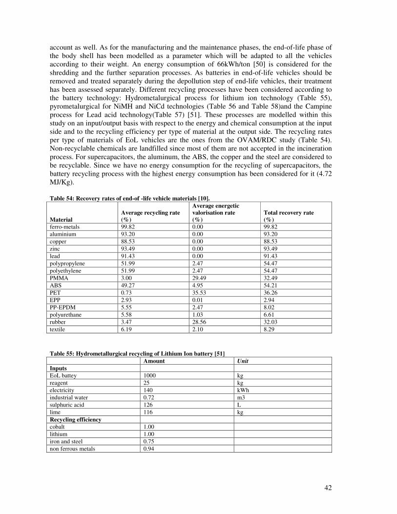
42
account as well. As for the manufacturing and the maintenance phases, the end-of-life phase of
the body shell has been modelled as a parameter which will be adapted to all the vehicles
according to their weight. An energy consumption of 66kWh/ton [50] is considered for the
shredding and the further separation processes. As batteries in end-of-life vehicles should be
removed and treated separately during the depollution step of end-life vehicles, their treatment
has been assessed separately. Different recycling processes have been considered according to
the battery technology: Hydrometalurgical process for lithium ion technology (Table 55),
pyrometalurgical for NiMH and NiCd technologies (Table 56 and Table 58)and the Campine
process for Lead acid technology(Table 57) [51]. These processes are modelled within this
study on an input/output basis with respect to the energy and chemical consumption at the input
side and to the recycling efficiency per type of material at the output side. The recycling rates
per type of materials of EoL vehicles are the ones from the OVAM/RDC study (Table 54).
Non-recyclable chemicals are landfilled since most of them are not accepted in the incineration
process. For supercapacitors, the aluminum, the ABS, the copper and the steel are considered to
be recyclable. Since we have no energy consumption for the recycling of supercapacitors, the
battery recycling process with the highest energy consumption has been considered for it (4.72
MJ/Kg).
Table 54: Recovery rates of end-of -life vehicle materials [10].
Material
Average recycling rate
(%)
Average energetic valorisation rate
(%)
Total recovery rate
(%)
ferro-metals 99.82 0.00 99.82
aluminium 93.20 0.00 93.20
copper 88.53 0.00 88.53
zinc 93.49 0.00 93.49
lead 91.43 0.00 91.43
polypropylene 51.99 2.47 54.47
polyethylene 51.99 2.47 54.47
PMMA 3.00 29.49 32.49
ABS 49.27 4.95 54.21
PET 0.73 35.53 36.26
EPP 2.93 0.01 2.94
PP-EPDM 5.55 2.47 8.02
polyurethane 5.58 1.03 6.61
rubber 3.47 28.56 32.03
textile 6.19 2.10 8.29
Table 55: Hydrometallurgical recycling of Lithium Ion battery [51]
Amount Unit
Inputs
EoL battey 1000 kg
reagent 25 kg
electricity 140 kWh
industrial water 0.72 m3
sulphuric acid 126 L
lime 116 kg
Recycling efficiency
cobalt 1.00
lithium 1.00
iron and steel 0.75
non ferrous metals 0.94

43
Table 56: Pyrometallurgical recycling of NiMH battery [51]
Amount Unit
Inputs
EoL battey 1000 kg
active carbon 1.67 kg
electricity 310 kWh
natural gas and propane 94.7 kg
process water 240 l
Recyccling efficiency
nickel-cobalt-iron 0.73
Table 57: Campine Lead acid battery recycling [51]
Amount Unit
Inputs
EoL battery 1000 kg
limestone 5.8 kg
iron scrap 4.0 kg
sodium hydroxide 350 kg
sodium nitrate 0.4 kg
sulphur 0.9 kg
iron chloride 0.9 kg
slag 150 kg
electricity 35.2 kg
natural gas 16.2 kg
coke 20.0 kg
process water 770 kg
Recycling efficiency
lead 1.00
sulphuric acid for reuse 0.44
Table 58: Pyrometallurgical recycling of NiCd battery [51]
Amount Unit Inputs EoL battey 1000 kg active carbon 1.67 kg electricity 1545 kWh propane/butane 170.6 kg process water 240 kg Recycling efficiency cadmium 0.90 nickel-iron 0.95
IV.15. Tank to Wheel (TTW) data
The Ecoscore database is the reference database for direct or Tank to-Wheel (TTW) emission
data for the CLEVER project. It contains fuel/energy consumption and emission data resulting
from the vehicle’s homologation procedure. The average CO2 emissions (g/km) as well as the
HC, SO2, NOx, CO, PM, CH4, N2O emissions (g/km) for each specific vehicle are contained in
the Ecoscore database. The consumption of liquid fuels is expressed in l/100 km, of gases in
m3/100 km and of electric energy in kWh/km. As the emissions are measured with the New
European Driving Cycle (NEDC) combining urban and extra-urban driving cycles, only
average emissions and fuel consumption are available in the Ecoscore database. Therefore
splitting up direct emissions into urban and extra-urban conditions is not possible. However, the
CLEVER LCA model is developed to assess the environmental impact of both urban and extra-
urban driving when the needed data will be available. The testing conditions under NEDC do

not include the additional fuel consumption of the cooling and the heating devices (Chasserot
M. 2007). The considered weight for the vehicle is
coolant, oils, fuel, spare wheels, tools and the driver (75 kg).(Directive 92/21/EEC
The Ecoscore database contains different vehicle technologies (petrol, diesel, battery electric,
hybrid electric, and flexi-fuel) and different vehicle
The modelling parameters of the life cycle of the different vehicles are extracted from the
Ecoscore database. A data analysis was performed to extract these parameters from the raw data
available in the Ecoscore database. Since the
modelling parameters are not fixed values but ranges. In the model, all the possible variations
of these parameters are taken into account, resulting in a variation of the considered impacts.
When including the frequencies of these values, one can match a triangular or uniform
distribution with the real distribution of the values.
this approach for a Euro 4 family car using petrol.
There are strong correlations between fuel consumption and vehicle weight, carbon dioxide and
sulphur dioxide. These parameters can be described as a linear function of fuel consumption,
multiplied with an ‘error’ distribution, expressing the difference between the linear equation
and the real distribution of the parameter. For the other emissions (HC, NOx, CO, PM,
and N2O), no satisfying correlation with fuel consumption was found. These emissions are
modelled as a triangular or a uniform distribution, matching the reality as closely as possible.
The chosen distributions have an important impact on the overall
conclusions of the data analysis are therefore interesting to discuss.
Fuel consumption, weight, CO2 and SO
other side, the Euro standard does not influence these parameters. Impacts o
and well-to-tank emissions do not change by introducing newer Euro standards. Tank
(TTW) emissions of CO2 and SO2 will also not change by introducing newer euro standards. On
the other hand it is noticeable that the Euro standard i
emissions. The higher the Euro standard, the lower HC, NO
are.
Figure 4: Range of the fuel consumption of the family petrol Euro 4 car
not include the additional fuel consumption of the cooling and the heating devices (Chasserot
M. 2007). The considered weight for the vehicle is the ‘in running order’ mass including
nt, oils, fuel, spare wheels, tools and the driver (75 kg).(Directive 92/21/EEC) The Ecoscore database contains different vehicle technologies (petrol, diesel, battery electric,
fuel) and different vehicle segment (see chapter I) of the Belgian fleet.
The modelling parameters of the life cycle of the different vehicles are extracted from the
Ecoscore database. A data analysis was performed to extract these parameters from the raw data
available in the Ecoscore database. Since the Belgian fleet includes a large variety of cars, the
modelling parameters are not fixed values but ranges. In the model, all the possible variations
of these parameters are taken into account, resulting in a variation of the considered impacts.
ng the frequencies of these values, one can match a triangular or uniform
distribution with the real distribution of the values. Figure 4 and Figure 5 give an example of
this approach for a Euro 4 family car using petrol.
There are strong correlations between fuel consumption and vehicle weight, carbon dioxide and
hese parameters can be described as a linear function of fuel consumption,
multiplied with an ‘error’ distribution, expressing the difference between the linear equation
and the real distribution of the parameter. For the other emissions (HC, NOx, CO, PM,
and N2O), no satisfying correlation with fuel consumption was found. These emissions are
modelled as a triangular or a uniform distribution, matching the reality as closely as possible.
The chosen distributions have an important impact on the overall result, preliminary
conclusions of the data analysis are therefore interesting to discuss.
and SO2 are highly dependent of the chosen segment. On the
other side, the Euro standard does not influence these parameters. Impacts of manufacturing
tank emissions do not change by introducing newer Euro standards. Tank
will also not change by introducing newer euro standards. On
the other hand it is noticeable that the Euro standard influences highly the other regulated TTW
emissions. The higher the Euro standard, the lower HC, NOx, CO, PM, CH4 and N2O emissions
: Range of the fuel consumption of the family petrol Euro 4 car
not include the additional fuel consumption of the cooling and the heating devices (Chasserot
the ‘in running order’ mass including
The Ecoscore database contains different vehicle technologies (petrol, diesel, battery electric,
of the Belgian fleet.
The modelling parameters of the life cycle of the different vehicles are extracted from the
Ecoscore database. A data analysis was performed to extract these parameters from the raw data
Belgian fleet includes a large variety of cars, the
modelling parameters are not fixed values but ranges. In the model, all the possible variations
of these parameters are taken into account, resulting in a variation of the considered impacts.
ng the frequencies of these values, one can match a triangular or uniform
give an example of
There are strong correlations between fuel consumption and vehicle weight, carbon dioxide and
hese parameters can be described as a linear function of fuel consumption,
multiplied with an ‘error’ distribution, expressing the difference between the linear equation
and the real distribution of the parameter. For the other emissions (HC, NOx, CO, PM, CH4
and N2O), no satisfying correlation with fuel consumption was found. These emissions are
modelled as a triangular or a uniform distribution, matching the reality as closely as possible.
result, preliminary
are highly dependent of the chosen segment. On the
f manufacturing
tank emissions do not change by introducing newer Euro standards. Tank-to-wheel
will also not change by introducing newer euro standards. On
nfluences highly the other regulated TTW
O emissions

Figure 5: Distribution of the fuel consumption of the family petrol Euro 4 car
As heavy metal emissions are not available in the Ecoscore database, emission factors in terms
of mg of substance per kg of burned fuel are gathered from the EMEP
inventory guidebook [49] for petrol and diesel cars (
Next to the Ecoscore database, some bio
Ecoinvent v2.0 have been collected as well. These emissions correspond to a range of vehicles
with a weight between 1300 and 1500 kg [
family car’ category according to the classification made in the CLEVER project. The
phases of E5 (petrol with 5% ethanol), methane from biogas, diesel with 5% RME, methanol,
petrol with 4% ETBE and petrol with 15% ETBE are included. The emission measurements
have been done with the New European Driving Cycle.
Furthermore, bio-fuel TTW emissions of the Volvo
C4 have been provided by the BIOSES project (
Table 59: heavy metal emissions of passenger car [
mg/kg burned petrol
cadmium 0.01
copper 1.70
chromium 0.05
nickel 0.07
selenium 0.01
zinc 1.00
lead 2.00E
mercury 7.00E
chromium IV 1.00E
Note: 0.2% of the emitted chrome is emitted as Chromium (IV
: Distribution of the fuel consumption of the family petrol Euro 4 car
As heavy metal emissions are not available in the Ecoscore database, emission factors in terms
of mg of substance per kg of burned fuel are gathered from the EMEP/CORINAIR emission
] for petrol and diesel cars (Table 59).
Next to the Ecoscore database, some bio-fuels’ Tank-to-Wheel data (Table 60) available in
have been collected as well. These emissions correspond to a range of vehicles
with a weight between 1300 and 1500 kg [52]. This range of vehicles corresponds to the ‘small
family car’ category according to the classification made in the CLEVER project. The
phases of E5 (petrol with 5% ethanol), methane from biogas, diesel with 5% RME, methanol,
petrol with 4% ETBE and petrol with 15% ETBE are included. The emission measurements
have been done with the New European Driving Cycle.
TW emissions of the Volvo F50, the Saab 9.5 BioPower and the Citroen
C4 have been provided by the BIOSES project (Table 61, Table 62and Table 63)
missions of passenger car [49]
mg/kg burned petrol mg/kg burned diesel
0.01
1.70
0.05
0.07
0.01
1.00
2.00E-03 1.10E-07
7.00E-05 2.00E-05
1.00E-04 1.00E-04
Note: 0.2% of the emitted chrome is emitted as Chromium (IV)
As heavy metal emissions are not available in the Ecoscore database, emission factors in terms
/CORINAIR emission
) available in
have been collected as well. These emissions correspond to a range of vehicles
]. This range of vehicles corresponds to the ‘small
family car’ category according to the classification made in the CLEVER project. The use
phases of E5 (petrol with 5% ethanol), methane from biogas, diesel with 5% RME, methanol,
petrol with 4% ETBE and petrol with 15% ETBE are included. The emission measurements
and the Citroen

46
Table 60: TTW emissions of bio-fuel vehicles [43].
Biomethane
(g/km)
E5
(g/km)
M100
(g/km)
B5
(g/km)
Petrol/ETBE15
(g/km)
Petrol/ETBE4
(g/km)
CO fossil 0.00E00 8.75E-04 0.00E00 6.09E-04 7.22E-04 7.47E-04
CO bio 4.46E-01 2.95E-02 9.31E-01 2.86E-02 3.31E-02 8.63E-03
CO2 fossil 0.00E00 189.00E00 0.00E00 166.00E00 177.00E00 183.00E00
CO2 bio 172.00E00 6.36E00 177.00E00 7.80E00 8.09E00 2.12E00
CH4 fossil 0.00E00 4.79E-03 0.00E00 3.37E-03 5.26E-03 5.44E-03
CH4 bio 4.51E-02 1.61E-04 1.44E-03 1.58E-04 2.41E-04 6.29E-05
NOx 2.06E-02 5.84E-05 3.84E-02 5.05E-01 3.56E-02 3.56E-02
PM 6.67E-04 1.98E-03 0.00E00 3.16E-02 1.00E-01 1.00E-01
N2O 8.66E-04 2.57E-03 2.60E-03 5.58E-03 1.33E-03 1.33E-03
SO2 8.95E-04 5.99E-03 0.00E00 5.25E-03 5.13E-03 5.04E-03
NMVOC 1.05E-02 5.84E-02 5.18E-02 1.29E-01 9.33E-02 9.33E-02
Benzene 7.62E-04 1.88E-03 2.74E-03 1.80E-03 8.89E-03 8.89E-03
Toluene 5.25E-03 8.71E-03 5.56E-03 4.15E-04 7.68E-03 7.68E-03
Xylene 5.39E-03 9.31E-03 5.28E-04 1.04E-03 7.68E-03 7.68E-03
Table 61: TTW emissions of the Citroen C4 using different blends of diesel [53].
Fuel consumption (l/100 km)
CO2 (g/km)
CO (g/km)
NOx (g/km)
HC (g/km)
diesel 5.79 152.4 3.4E-2 0.64 1.3 E-2
B5 6.03 159.1 2.8E-2 0.61 1.0 E-2
B10 5.94 156.0 2.3 E-2 0.58 1.0 E-2
B30 5.85 151.3 1.4 E-2 0.63 0.9 E-2
B100 6.07 149.7 1.2 E-2 0.71 1.6 E-2
Table 62: TTW emissioons of the Saab 9.5 BioPower using different blends of petrol [53]
Fuel consumption
(l/100 km)
CO2
(g/km)
CO
(g/km)
NOx
(g/km)
HC
(g/km)
diesel 10.49 247.74 0.26 3.66E-03 5.36E-03
E5 10.43 240.78 0.31 2.85E-03 5.40E-03
E10 10.67 239.71 0.18 2.92E-03 4.48E-03
E30 10.44 222.11 0.08 2.84E-03 2.27E-03
E85 13.30 212.97 0.05 2.61E-03 2.15E-03
Table 63: TTW emissions of the Volvo F50 using different blends of petrol [53]
Fuel consumption
(l/100 km)
CO2
(g/km)
CO
(g/km)
NOx
(g/km)
HC
(g/km)
Euro 95 7.40 175.63 0.21 17,33E-3 0.76E-3
E5 7.63 176.31 0.19 16.52E-3 0.69E-3
E10 7.93 178.07 0.21 20.02E-3 0.87E-3
E20 8.56 181.71 0.25 18.73E-3 0.99E-3
E85 12.16 192.90 0.15 18.73E-3 1.05E-3
Additionally, tailpipe emissions (Table 64) of two hydrogen vehicles have been collected from
[54, 55]. It is important to mention that contrarily to the other vehicle technologies, the
considered FCEV vehicle in this study is not yet homologated in Europe. Thus, an NEDC based
fuel consumption is not available for this vehicle. So, an US EPA (Environmental Protection
Agency) combined cycle based fuel economy of 60 miles (96.56 km) per kg has been
considered for the FCEV (Honda 2010). The Honda FCX Clarity has a driving range of 240
miles (386.23 km).

47
Table 64: TTW emissions of 2 prototype hydrogen vehicles [54], [55]
Air conditioning systems
According to [56], the use of an air conditioning system increases the vehicle’s fuel
consumption by 17.8 %, but this could vary according to the technology, the meteorological
conditions and the driving style. For example the extra consumption due to the air conditioning
ranges from 12 to 43% in an urban driving context according to the type of engine and the
driving behavior. Additionally, the extra consumption due to the weight of the air conditioning
system is about 8.2%.
IV.16 Conclusion
The LCI step of the CLEVER project has been performed thanks to a special data gathering
strategy. A list of all the relevant data sources and projects has been made during a detailed
literature review. Priority has been given to specific Belgian and European data. The Ecoinvent
v2.0 and Ecoscore databases have been the main data sources. Raw material production,
manufacturing, transport, fuel, energy, maintenance and Well-to-Wheel data are collected for
conventional and alternative vehicles. However, some adaptations have been made to avoid
repetition and to solve the problem with lack of data. Thus, for the manufacturing phase
complete LCI data of the VW Golf have been used to model a theoretical car which is used as a
parameter to model the other cars proportionately to their weight. For the emission control
technologies, only LCI data of a sedan catalytic converter are obtained. It is also important to
note that average Tank-to-Wheel data are considered instead of urban and extra-urban data
since the direct emissions come from the New European Driving Cycle.
Finally, the gathering of direct emissions of bio-fuel cars has been completed by the emission
measurement campaign which has been performed by the BIOSES project.
V. Life Cycle Impact Assessment After the completion of the LCI, the different elementary flows that are linked to a product
system need to be converted into environmental indicators. These indicators allow quantifying
and comparing the potential environmental impacts of the different product systems. This step
of the LCA is called Life Cycle Impact Assessment (LCIA). The LCIA has mandatory and
optional elements. The mandatory elements include the selection of impact categories, the
assignment of the elementary flows to the categories (classification) and the attribution of
factors to each elementary flow according to its relative contribution to the category
(Characterisation). The optional elements are the calculation of the magnitude of an impact
category relative to reference information (normalization) and the grouping of the different
impact indicators into a single score (weighting).[57]. However, weighting shall not be used for
comparative LCA studies intended to be disclosed to the public [58].
As required by [58], LCIA category indicators and characterisation models based on
international agreement should be used. In this perspective, the European commission via the
Vehicle Technology storage Fuel
[kg H2/km]
NOx
[g/km]
CO
[g/km]
CO2
[g/km]
NMHC
[g/km]
Ford P2000 H2-ICEV 1,5 kg at 248
bar 4.40E-03 4.60E-01 5.10E-03 8.70E-01 4.70E-03
Honda FCX
Clarity FCEV
3.92 kg at
345 bar 1.04E-02 0.00E+00 0.00E+00
0.00E+0
0
0.00E+0
0

48
Joint Research Centre (JRC) has initiated the International Reference Life Cycle Data System
(ILCD) in order to ‘provide governments and businesses with a basis for assuring quality and
consistency of life cycle data, methods and assessments’ [59]. In the framework of the ILCD activities,
an analysis of the existing LCIA methods has been performed [60]. In this analysis, the main existing
methodologies are described regarding the documentation, the general principals, the consistency across
a list of predefined impact categories and the interesting innovative aspects [60]. Finally, a list of
preselected LCIA methods has been produced (Table 65). These preselected LCIA methods will be
assessed in details by the ILCD team and a final list is expected for 2011.
Table 65: Pre-selection of characterisation models for further analysis [60]

49
In this study, it has been decided to use only LCIA methods preselected in the framework
of the ILCD activities and which are relevant for the specific context of automotive LCA.
The selected methods are:
• IPCC 2007 [61]
• Air acidification [62]
• Eutrophication [62]
• Mineral extraction [63]
• renewable and non renewable energy demand
• Respiratory effects (inorganics) [64]
As it can be noticed in Table 66 to Table 72, the most important and relevant elementary flows
are considered in the selected impact calculation methods. Endpoint methods, excepted
respiratory inorganics, have been used for all the selected impact categories.
For the specific cases of renewable and non renewable energy demand, the calculation method
has been developed by RDC-ENVIRONMENT with inputs from themselves and from the
Swiss Agency for the Environment, Forests and Landscape (BUWAL). The energy demand
(Table 69 and Table 70) includes all the types of primary energy involved in a product system.
It also includes the heating value of products, resources and materials.
The respiratory inorganics impact on human health (
Table 71) is particularly interesting in this study because it includes particulates, carbon
monoxide and nitrogen and sulphur based emissions. These emissions are among the pollutants
allowing clear differenction between vehicle technologies and fuels.
The IPCC 2007 (100a) method has been extended to biogenic CO2 and the CO2 uptake from the
air during the synthesis of the organic matter. A negative factor is attributed to the CO2 uptake.
The air acidification (Table 67) and eutrophication (Table 68) calculation expressed
respectively in kg SO2eq/kg and kg PO4eq/kg are from the CML 2001 methodology [62]. It
includes mainly nitrogen, sulphur and phosphorus based emissions. These two methods allow
performing a comprehensive assessment of the effect of the fertilizers for biofuels on one hand
and assessing the impact of the use of products and resources containing sulphur (e.g. crude
oil), phosphorus or nitrogen.
The mineral extraction damage (Table 72) expressed in MJ surplus/kg allows assessing the
additional energy requirement for further mining of the mineral resources in the future due to
the lower resource concentration. This method is particularly interesting for the manufacturing
phase of vehicles in general and the manufacturing of specific components ( battery, fuel cell,
hydrogen tank…) in particular.
Table 66: IPCC 2007 (100a) including biogenic CO2 and CO2 uptake from the air [61]
Elementary flows
Characterisation factor
(kg CO2 eq/kg)
CFC 12 (CCl2F2) 10900 CFC 113 (CFCl2CFCl2) 6130 HFC 23 (CHF3) 14800 HCFC 21 (CHCl2F) 210 CFC 11 (CFCl3) 4750 Chloroform (CHCl3) 756

50
HFC 134a (CF3CH2F) 4470 Hexafluoroethane (C2F6, FC116) 12200 Halon 1211 (CF2ClBr) 1890 CFC 114 (CF2ClCF2Cl) 10000 Sulphur Hexafluoride (SF6) 22800 Halon 1301 (CF3Br) 7140 HCFC 22 (CHF2Cl) 1810 Methan (biomass) 25 Nitrous Oxide (N2O) 298 Methane (CH4) 25 Carbon Dioxide (CO2, biomass) 1 Carbon Dioxide (CO2, in air) -1 Carbon Dioxide (CO2, fossil) 1 CFC 13 (CF3Cl) 14400 HCFC 124 (CHClFCF3) 609
Table 67: CML 2001 Air acidification [62]
Elementary flows Characterisation factor
(kg SO2eq/kg)
Sulphuric Acid (H2SO4) 0.65 Hydrogen Sulphide (H2S) 1.88 Hydrogen Fluoride (HF) 1.6 Ammonia (NH3) 1.6 Hydrogen Chloride (HCl) 0.88 Nitrogen Oxides (NOx as NO2) 0.5 Sulphur Oxides (SOx as SO2) 1.2 Nitrogen Dioxide (NO2) 0.5 Nitrogen Oxides (NOx as NO2) 0.5 Sulphur Dioxide (SO2) 1.2 Hydrogen Sulphide (H2S) 1.88
Table 68: CML 2001 eutrophication [62]
Elementary flows Characterisation factor
(kg PO4 eq/kg)
ammonia 0,35
chemical oxygen demand 0,022
nitrogenous matter 0,42
nitrous oxide 0,27
phosphates 1.00
Phosphorus, total 3,06
phosphorus pentoxide 1,34
nitrate 0,10
nitrite 0,10
nitrogen 0,42
nitrogen dioxide 0,13
nitrogen monoxide 0,20
nitrogen oxides 0,13
�
Table 69: Non renewable energy (BUWAL/RDC)
Elementary flows Characterisation factor Unit
Peat 25 MJeq/kg
Coal (in ground) 19 MJeq/kg
Oil (in ground) 45,6 MJeq/kg
Lignite (in ground) 9,5 MJeq/kg
Natural Gas (in ground) 48,1 MJeq/kg
Uranium (U, ore) 451000 MJeq/kg
Unspecified Fuel Energy 1 MJeq/MJ

51
Table 70: Renewable energy (BUWAL/RDC)
Elementary flows Characterisation factor Unit
Wood 20 MJeq/kg
Water Potential energy 1 MJeq/MJ
Non fossil Fuel Energy 1 MJeq/MJ
Solar energy 1 MJeq/MJ
Wind enery 1 MJeq/MJ
Geothermal energy 1 MJeq/MJ
Table 71: Impact 2002+ respiratory inorganics (endpoints) [64]
Elementary flows Normalised damage factors
(Impact 2002+ point)
Ammonia (NH3) 1.20E-02
Carbon Monoxide (CO) 1.03E-04
Nitrogen Dioxide (NO2) 1.25E-02
Nitrogen Oxides (NOx as NO2) 1.25E-02
Sulphur Oxides (SOx as SO2) 7.69E-03
Sulphur Dioxide (SO2) 7.69E-03
Particulates (PM 2.5) 9.86E-02
Carbon monoxide (biomass) 1.03E-04
Table 72: Eco-indicator 99 Hieratchist, Resources, Mineral extraction damage (midpoints) [63]
Elementary flows MJ surplus/kg Aluminum in bauxite 2.38 Chromium (Cr, ore) 0.9165 Copper (Cu, ore) 36.7 Iron (Fe, ore) 0.051 Lead (Pb, ore) 7.35 Manganese (Mn, ore) 0.313 Mercury (Hg, ore) 165.5 Molybdenum (Mo, ore) 41 Nickel (Ni, ore) 23.75 Tin (Sn, ore) 600 Zinc (Zn, ore) 4.09
VI. The RangeLCA software The range-based modeling system possesses some innovative attributes which allow improving
the reliability of the results. In statistical viewpoint, this approach employs the use of random
variables instead of average values .Compared to a classic LCA tool; it allows assessing all the
possible cases instead of one single case. The random values are modeled with parameters
which include all the values between the extreme values by giving an occurrence probability to
each data. According to the situation to be modeled different type of distribution functions can
be chosen. One of the main assets of the RangeLCA software is the possibility to express a link
between two life cycle steps by the prior links in such away that each variation or change in the
previous steps will be automatically taken into account and all different situations will be
included in one single model. Thus the sensitivity analysis of all the parameters will be
systematically incorporated.
Furthermore, the range-based modeling system allows comparing two systems with
simultaneously varying parameters. In fact, while comparing two different systems within an
LCA, two types of variations could happen: Variation of the results due to the variation of
common parameters to the two systems and another variation of the results due to the variation
of parameters which are specific to each system. Thus, to achieve a real comparison of the two

52
systems one should identify and assess the variability of system specific parameters which
allow distinguishing the specificities of each system. It produced results integrate a set of
possible combinations for the various parameters and data in order to take into account possible
synergy and compensation effects
VII. Results and discussion The LCA results of this study should be interpreted with caution. The objective of this study is
not to compare different technological options (hybrid, FCEV, BEV, ICE…) of one single
vehicle but to compare different existing vehicle technologies of the Belgian fleet. More
specifically, the compared vehicles do not have the same size or the same energy consumption
but they are from the same market segment and are being used for the same purpose by the end-
user. The comparison of different family car technologies shows that the climate impact is
highly influenced by the vehicle technology, the type of fuel and the type of feedstock used to
produce the fuel (Figure 6). One can notice in the Figure 6 that the sugar cane based E85
vehicle has the lowest greenhouse effect. This is due essentially to the benefit of the CO2 uptake
from the air during the production of the sugar cane. Additionally, the electricity used in the
sugar cane fermentation plant is produced with the bagasse obtained after the crushing of the
sugar cane. However this good score of the E85 highly depends on the feedstock type and e.g
shifting from sugar cane to sugar beets will increase by more than three times the impact of the
E85 vehicle (Figure 6). After the sugar cane based E85 vehicle, the BEV using the Belgian
supply mix electricity has the lowest greenhouse effect. This good score of the BEV can be
explained by the fact that 55% of the Belgian production mix electricity is nuclear and the fact
that BEV is an exhaust emission free vehicle. Despite the low greenhouse effect of the BEV,
the contribution of the lithium ion battery to the overall impact is still higher. However, a big
share of the impact of the lithium battery is balanced by the benefit of the recycling. Like the
BEV, the FCEV is also an exhaust emission free vehicle but it has a greenhouse effect higher
than the BEV and comparable to the B100 (RME) one (Figure 6). The difference between the
FCEV and the BEV is due essentially to the fact that the hydrogen is produced with natural gas
when more than the half of the Belgian electricity is nuclear. Contrarily to the sugar cane based
E85, the B100 (RME) production is almost greenhouse neutral. Indeed, the benefit of the CO2
uptake from the air during the rape production is balanced by the effect of the intensive
agricultural practices such as the fertilizing and the machinery.
Another interesting finding of this study is the good climate impact score of CNG vehicles in
comparison to alternative vehicles such as hybrid and LPG. In fact, the natural gas production is
less energy intensive and pollutes less than the production of petrol and propane/butane based
LPG. Additionally, natural gas also has a good combustion efficiency. However, the benefit of
fuel saving of hybrid cars (lower TTW impact) compared to ICE vehicles is clearly identified in
the Figure 6. The relatively higher greenhouse effect of the LPG car can be explained by the
fact that the LPG is modeled with propane/butane combined with a liquefaction process. The
use of flare gas to produce LPG would reduce this impact. In general, for alternative vehicles
such as FCEV and BEV the recycling of specific components such as the fuel cell or the lithium
battery has a big environmental benefit. Furthermore the type of feedstock and the conversion
technology for alternative fuels (bio-fuel, hydrogen…) have a strong influence on the GHE of
the vehicles.
In order to have a deeper understanding of the results of this study, the LCA model has been
run 1000 times with different values chosen randomly between the minimum and the maximum
of all parameters modeled as a range. However extreme values corresponding to 2% of the
iterations have been excluded. Thanks to this approach, the effect of the simultaneous variation
of the vehicle weight, the energy consumption and the emissions has been assessed. No weight

53
variation has been considered for specific cases (FCEV, BEV, E 85, CNG and B100) where
only one vehicle is available. However, the errors on the measurements of the fuel consumption
and the direct emissions have been included for these vehicles. As a consequence, vehicle
technologies with large variety of brands and models (Petrol, Diesel, LPG and Hybrid) will
have a wide spread of LCA results. With such an approach, stronger conclusions are drawn
because the worst case of a given technology can be compared to the most favorable case of
another one. For example, one can notice on the Figure 6 that the considered BEV powered
with the Belgian electricity is not only better than the other fossil fuel vehicles in average but
also better than the smallest fossil fuel vehicles of its segment. Thanks to this iterative
approach, the overlaps between the different technologies are identified. On a policy
perspective, the decision makers can use these kinds of results to determine for which groups of
vehicles they can take the same policy measures or on the contrary to identify for which groups
specific measures are necessary.
Figure 6: Comparative GHE assessment of family car technologies
On the Figure 7, different scenarios of BEV using different types of electricity have been
compared to assess the influence of the electricity production technology on the LCA results of
BEVs. The BEVs powered with windpower, hydropower or nuclear power appear to have very
low greenhouse effect. They are followed by the scenarios of the Belgian mix electricity and the
natural gas electricity which also have very low greenhouse effect in comparison to diesel and
petrol vehicles. However, extreme scenarios in which BEVs are powered with oil or coal
electricity appears to have climate impacts which are comparable to the ones of diesel cars. In
average, the greenhouse effect of petrol cars is still higher than the one of BEVs powered with
oil or coal electricity. Nevertheless, The error bars (Figure 7) show that small petrol cars within
the family car segment can have greenhouse effect which is comparable to a BEV powered with
coal or oil electricity.
Family car: GHE ( ton CO2eq/lifetime driven distance)
-60
-40
-20
0
20
40
60
80
100
BEV
(BE m
ix)
FCEV
(SM
R)
CN
G, E
uro
4
Hyb
rid, E
uro
4
E85 (S
.can
e)
LPG ,
Euro 4
Die
sel,
Euro 4
Die
sel,
Euro
5
B10
0 (RM
E)
Petro
l, Eur
o 4
Petro
l, Eur
o 5
E85 (S
.bee
ts)
Hydrogen Tank
Fuel Cell
Lithium Ion
batteryNiMH battery
TTW
WTT
Raw Materials
Assembly eq.car
Maintenance
Lead battery
Transport
Eof lead battery
End of life (EoL)
EoL NiMH
BatteryEoL Li battery
EoL Fuel Cell
GHE Total

54
Figure 7: Sensitivity of the GHE impact of BEV to the type of electricity production
Close to the GHE, the respiratory effects of the different family car technologies have been
compared (Figure 8). Contrarily to the GHE, the E85 sugar cane technology has the worst score
for the respiratory effects (inorganics). This is due mainly to the burning of the sugar cane field
before the harvest. The main pollutants emitted during the field burning are Carbone monoxide,
methane and particles [65]. However, a regulation allowing a progressive shift from manual
harvesting (with field burning) to automatic harvesting (without field burning) is being
implemented in Sao Paolo by 2021 [66]. It is then followed by the RME vehicle. This high
respiratory effect of the RME is due mainly to the emission of ammonia and nitrogen oxides
which are directly linked to the use of nitrogen based mineral fertilizers. Additionally, the bio-
diesel vehicle emits more nitrogen oxides than the corresponding diesel vehicle.
The best score in this impact category goes to the CNG vehicle. The production of the natural
gas has relatively low emission for all the considered pollutants in this category. This is also
true for the direct emissions of the CNG vehicle. The CNG technology is followed by the BEV.
The FCEV has a respiratory effect lower than the ICE vehicles but slightly higher than the
BEV. Without recycling of the fuel cell, the FCEV would have the worst score for this impact
after the E85 and the RME vehicles.
GHE (ton CO2eq)
-1.E+01
0.E+00
1.E+01
2.E+01
3.E+01
4.E+01
5.E+01
6.E+01
7.E+01
8.E+01
9.E+01
BEV, w
ind
BEV, h
ydro
BEV, n
ucle
arBE
V, BE m
ix
BEV,B
E mix
(NiC
d)BE
V, gas
BEV, o
ilBE
V, coal
Die
sel E
uro 5
Die
sel E
uro 4
Petrol E
uro 5
Petrol E
uro 4
NiCd battery
EOF NiCd
WTT
TTW
Transport
Raw Materials
Maintenance
Lithium Ion battery
Lead acid battery
EOL Li battery
Eof lead acid battery
End of life
Assembly eq.car
GHE Total

55
Figure 8: Respiratory effects of different family car technologies
After the overall vehicle technology comparison within the family car segment, a list of
reference vehicles which are considered to be more representative of their respective segment
has been made. The aim is to perform a fair comparison between equivalent vehicles because
sometimes a limited number of vehicles with high weight or high fuel consumption can
influence the average result of a full segment for a given technology. The individual
comparison of the reference vehicle for GHE (Figure 9) gives the same ranking trend as in the
Figure 6 for the different vehicle technologies. However, the Figure 9 shows that the
differences between the different technologies, especially the difference between petrol and
diesel, are smaller than in the overall comparison. Moreover, the Figure 9 shows that the
segment also has a big influence on the LCA results. For example, a petrol family car will have
a lower GHE than a hybrid SUV.
Repiratory effect (inorganics)
-3
-2
-1
0
1
2
3
4
5
6
7
BE
V (B
E m
ix)
FCE
V S
MR
CN
G, E
uro 4
Hybri
d, Euro
4
E85
(S.c
ane)
LPG
, Euro
4
Die
sel,
Euro
4
Die
sel,
Euro
5
B100
(RM
E)
Petro
l, Euro
4
Petro
l, Euro
5
E85
(S.b
eets
)
Imp
ac
t 2
00
2+
po
ints
Tire/Brake abrasion
Hydrogen Tank
Fuel Cell
Lithium Ion battery
NiMH battery
TTW
WTT
Raw Materials
Assembly eq.car
Maintenance
Lead battery
Transport
Eof lead battery
End of life (EoL)
EoL NiMH Battery
EoL Li battery
EoL Fuel Cell
Total

56
Figure 9: GHE of different comparable individual vehicle technologies and segments
VIII. Scientific validation of the Ecoscore approach
VIII.1 Introduction
The Vrije Universiteit Brussel, ULB and VITO have developed the Ecoscore methodology [14],
a well-to-wheel environmental vehicle rating tool. This tool has been developed to apply in
different policy measures for the Flemish government to promote the purchase and use of
cleaner vehicles. Since this tool had to be transparent and easily applicable on a policy level,
emission and fuel consumption data had to be available for all vehicles on the Belgian market.
The LCA methodology however, requires an extensive set of emission data per vehicle, which
is not always easy to retrieve. The more pragmatically Ecoscore tool is therefore based on a
‘simplified’ LCA methodology, where only the airborne well-to-wheel emissions are taken into
account, but which allows the calculation of an environmental impact for each individual
vehicle.
In this chapter, a comparison will be made between the Ecoscore and LCA results of different
vehicle technologies and vehicles of different ages, to assess the influence of neglecting the
impact of the manufacturing, maintenance and end-of-life phases of a vehicle and hence
validate the Ecoscore approach.
GHE (reference Vehicles)
0
10
20
30
40
50
60
70
80
90
City
, Pun
to, C
NG
City
, Pun
to, D
iese
l
City
, Pun
to, L
PG
City
, Pun
to, p
etro
l
Niss
an L
eaf ,
ele
ctric
Smal
l Fam
ily ,
Ford F
ocus,
Die
sel
Smal
l Fam
ily ,
Ford F
ocus,
LPG
Smal
l Fam
ily ,
Ford F
ocus, p
etro
l
Fam
ily c
ar, T
oyot
a pr
ius, h
ybrid
fam
ily c
ar, V
olvo
S40, D
iese
l
fam
ily c
ar, V
olvo
S40, L
PG
fam
ily c
ar, V
olvo
S40, p
etro
l
SUV
, Lex
us, H
ybrid
SUV
, Mer
cedes
, LPG
SUV
, Mer
cedes
,Die
sel
SUV
, Mer
cedes
, Pet
rol
ton
ne
CO
2q
/life
tim
e

57
VIII.2 Ecoscore methodology
The Ecoscore methodology has been developed with the aim to calculate the environmental
impact for every individual vehicle and to compare different vehicle technologies in an
objective way. Ecoscore is an environmental score, in which different damage effects are taken
into account: climate change, air quality depletion (health impairing effects and effects on
ecosystems) and noise pollution. The methodology is based on a well-to-wheel analysis, which
means that besides tailpipe emissions, also the air pollution caused by the production and
distribution of the fuel is taken into account. This allows a comparison of different vehicle fuels
and technologies.
The Ecoscore methodology can be considered as a simplified LCA, since only the well-to-
wheel environmental impact is considered, while the impacts of the production and end-of-life
stages of the vehicle itself are neglected. The environmental evaluation of a vehicle through this
methodology is being done according to a sequence of five steps, similar to those used in a
standardised LCA: inventary, classification, characterisation, normalisation and weighting.
In the first step of the inventary, the direct (associated with the use of the vehicle) and indirect
emissions (due to production and distribution of the fuel) associated with the vehicle are
collected. Direct of tank-to-wheel emission and fuel consumption data are based on
homologation data collected by Febiac and DIV (Federal service for vehicle registrations) and
which can be consulted on www.ecoscore.be. Indirect or well-to-tank emission data have been
obtained from the MEET 1995 study [67], complemented with Electrabel data for electricity
production. In the calculation of the total impact of the vehicle, the exposition of the receptors
is taken into account by giving the indirect emissions a smaller weight than the direct emissions
(with an exception for greenhouse gases, since they have a global effect). Once the emissions
have been calculated, their contribution to the different damage categories (climate change, air
quality depletion and noise) are analysed in the classification and characterisation step. The
contributions of the different greenhouse gases to global warming are calculated using global
warming potentials (GWP), as defined by the Intergovernmental Panel on Climate Change
(IPCC). External costs, based on the EU ExternE project [68], are used for the inventoried air
quality depleting emissions. Noise pollution is expressed in dB(A), a decibel scale with A-
weighting to take the sensitivity of human hearing into account. To quantify the relative
severity of the evaluated damages of each damage category, a normalisation step based on a
specific reference value is performed. The reference point is the damage associated with a
theoretical passenger vehicle of which the emission levels correspond with the Euro 4 emission
target levels for petrol vehicles, a CO2 emission level of 120 g/km and a noise level of 70
dB(A). In a final step, the normalised damages are weighted before they can be added to
become the “total environmental impact”. These weighting factors reflect policy priorities and
decision maker’s opinions. An overview of the methodology is presented in . To obtain results
situated between 0 (infinitely polluting) and 100 (emission free and silent vehicle), the total
environmental impact (TI or Total Impact) is rescaled to the final Ecoscore indicator. The
reference vehicle corresponds to an Ecoscore value of 70. The transformation is based on an
exponential function, so it cannot deliver negative scores:
Ecoscore = 100*exp(-0,00357*TI)

58
Figure 10: Overview of the Ecoscore methodology [14].
VIII.2 Vehicle selection
Three types of comparisons were made to validate the Ecoscore approach. For both petrol and
diesel cars, the environmental performance was followed over the different Euro standards and
hence vehicle ages. Another analysis includes the comparison of different vehicle technologies
which are available on the market, all complying with the latest Euro 5 standard: petrol, diesel,
LPG, CNG, petrol hybrid and BEV.
Based on the Ecoscore database of January 2010, a selection was made of comparable vehicles
from different vehicle technologies (Table 73). The Volkswagen Golf was used as a reference
model since it is available since Euro 2 and is still a popular car on the Belgian market. When
no VW Golf model was available, comparable cars have been chosen from the database. For
CNG the Opel Zafira was used, for BEV the Nissan Leaf and for the petrol hybrid the Toyota
Prius. For these vehicles, the LCA results were calculated, making a distinction between the
different life cycle phases, as well as the Total Impact. This was done for three impact
categories: greenhouse effect, impact on human health and impact on ecosystems.
Table 73: Selected vehicles with their fuel consumption, emissions, Ecoscore and Total Impact (TI).
Fuel/
Technology
Euro
standard
Car model Fuel
consumption
[l/100km]
CO2
[g/km]
CO
[g/km]
HC
[g/km]
NOx
[g/km]
SO2
[g/km]
PM
[g/km]
N2O
[g/km]
CH4
[g/km]
Ecoscore TI
Euro 1 Chrysler Stratus 8,2 196 2,720 0,530 0,440 0,00124 0 0,027 0,020 48,93 200,42
Euro 2 Volkswagen Golf 8,9 213 2,200 0,275 0,225 0,00134 0 0,013 0,020 52,36 181,39
Euro 3 Volkswagen Golf 9,0 215 2,300 0,200 0,150 0,00136 0 0,005 0,020 54,02 172,66
Euro 4 Volkswagen Golf 8,1 194 1,000 0,100 0,080 0,00122 0 0,005 0,020 58,90 148,34
Euro 5 Volkswagen Golf 6,2 144 0,286 0,028 0,045 0,00094 0 0,005 0,020 67,05 112,05
Euro 1 Jeep Cherokee 9,5 251 2,720 0,100 0,870 0,00162 0,14 0,002 0,010 20,96 438,12
Euro 2 Volkswagen Golf 6,2 164 1,000 0,070 0,630 0,00105 0,08 0,005 0,010 36,81 280,22
Euro 3 Volkswagen Golf 5,4 143 0,640 0,060 0,500 0,00092 0,05 0,008 0,010 46,68 213,62
Euro 4 Volkswagen Golf 5,2 137 0,129 0,013 0,237 0,00088 0,02 0,008 0,010 60,50 140,96
Euro 5 Volkswagen Golf 4,9 128 0,245 0,040 0,136 0,00083 0,001 0,008 0,010 70,22 99,10
LPG Euro 5 Volkswagen Golf 7,1 169 0,330 0,032 0,012 0,00117 0 0,005 0,020 71,19 95,29
CNG Euro 5 Opel Zafira 7,8 139 0,215 0,065 0,022 0 0 0,005 0,124 73,56 86,10
Hybrid Euro 5 Toyota Prius 3,9 89 0,258 0,058 0,006 0,00059 0 0,005 0,020 77,40 71,81
BEV Euro 5 Nissan Leaf 0,15 kWh/km 0 0,000 0,000 0,000 0 0 0 0,000 85,96 42,42
Petrol
Diesel

59
VIII.3 Comparison of Total Impact (Ecoscore) and LCA results
In the following figures, a comparison is made between Total Impact and LCA results for three
impact categories: greenhouse effect, impact on human health and impact on ecosystems.
Figure 11 shows the results of this comparison for petrol cars of different ages according to the
Euro standard. For the three assessed impact categories, the same trend is seen for TI as for
LCA. The impact on human health and ecosystems decreases with the age of the petrol car, if
assessed with LCA or TI. For greenhouse effect, the Euro 2 and Euro 3 petrol car have a higher
impact than Euro 1, 4 and 5 due to the higher TTW emissions of these cars, which is directly
related to the higher fuel consumption and hence CO2 emissions of these vehicles (see Table
73). Since their regulated emissions (CO, NOx, HC) decrease according to the emission
standards, their impact on human health and ecosystems is lower than for the Euro 1 petrol car.
Between these different vehicles, the impact due to manufacture, maintenance and end-of-life
remains almost constant. The differences are almost entirely due to the well-to-wheel emissions
of the vehicle.
Figure 12 gives a similar comparison as was shown in Figure 11, but this time for diesel cars of
different ages. Again the LCA and TI results display the same trend between the different cars.
The impact on greenhouse effect, health and ecosystems decreases towards more recent cars.
This can be almost entirely assigned to the well-to-wheel emissions, since the contribution of
the manufacture, maintenance and end-of-life phases remains quite stable over time.
The last set of graphs (Figure 13) gives a comparison between different vehicle
technologies/fuels, all complying with the Euro 5 emission standard. The impact on greenhouse
effect is the lowest for the BEV, followed by the hybrid vehicle. The same ranking of vehicle
technologies results from the LCA and TI analysis. The WTT and TTW phases are the largest
contributors for this impact category. For the impact on human health and ecosystems, the other
life cycle phases play a more important role, especially for the alternative vehicle technologies.
The larger impact of the manufacturing phase for the CNG car is due to the higher weight of
this car compared to the VW Golf. The larger impact on health and ecosystems of the
manufacturing and end-of-life of the hybrid and BEV are due to the impact of the battery of
these cars. This change in the contribution of the different life cycle phases has created some
changes in the relative position of the vehicles, especially for human health. The CNG car has
the lowest impact (TI and LCA) on human health due to the very low WTW emissions. Also for
the impact on ecosystems, the CNG car has the lowest impact, together with the BEV.
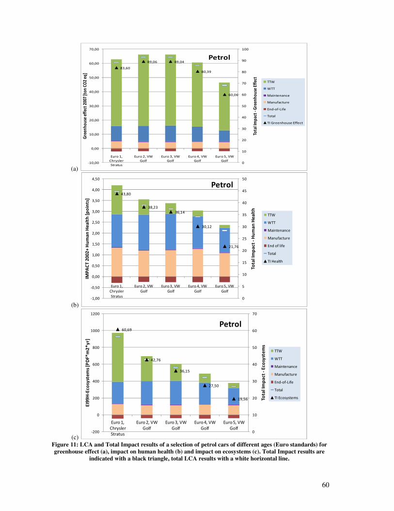
60
(a)
(b)
(c) Figure 11: LCA and Total Impact results of a selection of petrol cars of different ages (Euro standards) for
greenhouse effect (a), impact on human health (b) and impact on ecosystems (c). Total Impact results are
indicated with a black triangle, total LCA results with a white horizontal line.
83,60
89,06 89,04
80,39
60,06
0
10
20
30
40
50
60
70
80
90
100
-10,00
0,00
10,00
20,00
30,00
40,00
50,00
60,00
70,00
Euro 1,
Chrysler
Stratus
Euro 2, VW
Golf
Euro 3, VW
Golf
Euro 4, VW
Golf
Euro 5, VW
Golf
Tota
l Im
pac
t -G
reen
ho
use
Eff
ect
Gre
enh
ou
se e
ffec
t 20
07 [t
on
CO
2 eq
]TTW
WTT
Maintenance
Manufacture
End-of-Life
Total
TI Greenhouse Effect
Petrol
43,80
38,23
36,14
30,12
21,76
0
5
10
15
20
25
30
35
40
45
50
-1,00
-0,50
0,00
0,50
1,00
1,50
2,00
2,50
3,00
3,50
4,00
4,50
Euro 1,
Chrysler
Stratus
Euro 2, VW
Golf
Euro 3, VW
Golf
Euro 4, VW
Golf
Euro 5, VW
Golf
Tota
l Im
pa
ct -
Hu
ma
n H
ea
lth
IMP
AC
T 2
00
2+
Hu
ma
n H
ea
lth
[p
oin
ts]
TTW
WTT
Maintenance
Manufacture
End of life
Total
TI Health
Petrol
60,69
42,76
36,15
27,50
19,56
0
10
20
30
40
50
60
70
-200
0
200
400
600
800
1000
1200
Euro 1,
Chrysler
Stratus
Euro 2, VW
Golf
Euro 3, VW
Golf
Euro 4, VW
Golf
Euro 5, VW
Golf
Tota
l Im
pa
ct -
Eco
syst
em
s
EI9
9H
-Eco
syst
em
s [P
DF*
m2
*y
r]
TTW
WTT
Maintenance
Manufacture
End-of-Life
Total
TI Ecosystems
Petrol

61
(a)
(b)
(c)
Figure 12: LCA and Total Impact results of a selection of diesel cars of different ages (Euro standards) for greenhouse effect (a), impact on human health (b) and impact on ecosystems (c). Total Impact results are
indicated with a black triangle, total LCA results with a white horizontal line.
100,50
66,09
58,0255,65
52,10
-50
-30
-10
10
30
50
70
90
110
-10
0
10
20
30
40
50
60
70
80
Euro 1, Jeep
Cherokee
Euro 2, VW Golf Euro 3, VW Golf Euro 4, VW Golf Euro 5, VW Golf
Tota
l Im
pa
ct -
Gre
en
ho
use
Eff
ect
[p
oin
ts]
Gre
en
ho
use
Eff
ect
20
07
[to
n C
O2
eq
]TTW
WTT
Maintenance
Manufacture
End-of-Life
Total
Diesel
224,62
131,41
86,55
40,77
13,37
-50
0
50
100
150
200
250
-1
0
1
2
3
4
5
6
7
Euro 1, Jeep
Cherokee
Euro 2, VW Golf Euro 3, VW Golf Euro 4, VW Golf Euro 5, VW Golf
Tota
l Im
pa
ct -
Hu
ma
n h
ea
lth
[p
oin
ts]
IMP
AC
T 2
00
2+
Hu
ma
n H
ea
lth
[p
oin
ts]
TTW
WTT
Maintenance
Manufacture
End-of-Life
Total
TI Health
Diesel
100,66
71,39
57,72
33,21
23,30
0
20
40
60
80
100
120
-200
0
200
400
600
800
1000
1200
1400
1600
1800
Euro 1, Jeep
Cherokee
Euro 2, VW
Golf
Euro 3, VW
Golf
Euro 4, VW
Golf
Euro 5, VW
Golf
Tota
l Im
pac
t -E
cosy
stem
s [p
oin
ts]
EI99
H-E
cosy
stem
s [P
DF*
m2*
yr]
TTW
WTT
Maintenance
Manufacture
End-of-Life
Total
TI Ecosystems
Diesel

62
(a)
(b)
(c) Figure 13: LCA and Total Impact results of a selection of different vehicle technologies for greenhouse
effect (a), impact on human health (b) and impact on ecosystems (c). Total Impact results are indicated with
a black triangle, total LCA results with a white horizontal line.
60,06
52,10
66,35
60,63
37,47
15,18
-15
-5
5
15
25
35
45
55
65
-10
0
10
20
30
40
50
60
Petrol (Golf) Diesel (Golf) LPG (Golf) CNG (Zafira) Hybrid (Prius) EV (Leaf)
To
tal Im
pa
ct
-G
ree
nh
ou
se E
ffe
ct
[po
ints
]
Gre
en
ho
use
Eff
ect
20
07
[to
n C
O2
eq
]
TTW
WTT
Maintenance
Manufacture
End-of-Life
Total
TI Greenhouse
Effect
21,76
13,37
8,477,17
14,41
8,44
-20
-10
0
10
20
30
40
50
-1
-1
0
1
1
2
2
3
3
Petrol (Golf) Diesel (Golf) LPG (Golf) CNG (Zafira) Hybrid (Prius) EV (Leaf)
Tota
l Im
pa
ct -
Hu
ma
n H
ea
lth
[p
oin
ts]
IMP
AC
T 2
00
2+
Hu
ma
n H
ea
lth
[p
oin
ts]
TTW
WTT
Maintenance
Manufacture
End-of-Life
Total
TI Health
19,56
23,30
9,81
6,96
10,26
8,80
-10
-5
0
5
10
15
20
25
-200
-100
0
100
200
300
400
500
Petrol (Golf) Diesel (Golf) LPG (Golf) CNG (Zafira) Hybrid (Prius) EV (Leaf) Tota
l Im
pa
ct
-E
co
syst
em
s [p
oin
ts]
EI9
9H
-E
co
syst
em
s [P
DF*
m2
*y
r]
TTW
WTT
Maintenance
Manufacture
End-of-Life
Total
TI Ecosystems

63
IX. Optimal time for replacement
IX.1 Introduction
The energy consumption and the exhaust emissions of new vehicles have decreased
considerably the last years, driven by European emission standards, technological exhaust
treatment improvements and efficient engine technologies. These technological transitions
towards a more sustainable transportation system are encouraged by two main drivers: the
availability of energy sources (political and economical dependence on oil producing countries
and the depletion of the reserve base of fossil fuels) and the negative environmental aspects of
the current transport system [69].
A persistent transition towards a more sustainable transportation sector will involve a mixture
of several options such as: encouraging modal shifts (walking, cycling, public transport), cleaner
vehicle technologies, changing driving behaviour, and controlling the need for motorized
transportation [14].
A way to improve the environmental impact of the transport sector is by replacing old
inefficient vehicles by newer ones. A passenger car in Belgium has a lifetime driven distance
(LTDD) of 230,500 km, which corresponds to 13.7 years [13]. To cover this distance, a smaller
impact on the environment could be obtained by replacing this car before its lifetime with an
environmentally friendlier car. Vehicle replacement is normally driven by economic concerns.
This chapter gives insights in how to introduce environmental aspects in automobile
replacement policies. These policies aim at accelerating the adoption of cleaner vehicles by
taking old vehicles out of the fleet, while supporting the vehicle industry. A scrappage policy
must take the whole life cycle of a vehicle into account. Scrapping an old vehicle and
manufacturing a new one creates additional environmental impacts which must be taken into
consideration. Results of a Life Cycle Assessment (LCA) will be used to check how the Belgian
fleet can evolve towards a greener composition.
IX.2 Methodology
Life Cycle Assessment is a cradle-to-grave approach to determine the total environmental
impact of a product during its life cycle. It includes the extraction of raw materials,
manufacturing, transportation, use and disposal. Since the 90s, LCA is a standardized
methodology [57], [58]. It consists of four phases: goal definition and scoping, inventory
analysis, impact assessment and interpretation.
The goal of this study is to adapt the vehicle fleet to a more ecological composition, in function
of the LCA results. This analysis will be based on the comparison of the well-to-wheel
emissions with the cradle-to-grave (manufacturing, dismantling, recycling and waste treatment)
emissions for vehicles with different ages, Euro standards and technologies. Optimizing
vehicle’s LTDD causes an LCA challenge, combining two contradictory environmental
engineering concepts. Letting a vehicle have a longer use phase avoids specific impacts during
manufacturing, such as mineral extraction damage and energy usage. Product life extension is a
well known DfE (design for environment) strategy [70], [71]. To expand the LTDD the focus
will lie on durability and maintenance. In this case the policy advise would be to replace the old
vehicle as late as possible.

64
Conversely, replacement of an old vehicle with a new, more efficient one, can lower the
impacts introduced during the use phase. Depending on the level of benefit, the policy advise
would be to replace the old car as soon as possible. In this case, the focus will lie on the
development of cleaner vehicle technologies [72].
The optimal time to replace a car depends highly on the market availability of cleaner vehicles.
If an optimization, is to tackle greenhouse gases and there is no car on the market which
consumes considerately less fuel, there is no reason to replace the old vehicle. Moreover, the
CO2 emissions introduced during scrapping an old car and manufacturing a new one would
increase the overall impact on global warming.
To calculate in this case the optimal time of replacement [72] developed a methodology which
takes future developments of cleaner vehicles into account. Today there are cleaner, energy
efficient vehicle technologies available [73]. In this chapter it is discussed what can be done to
optimize the environmental impact of a vehicle today. To differentiate between vehicle
technologies it is investigated how long it takes a new car to have an environmental return on
investment. If we replace an old car today, how fast are we going to feel the benefits? This
period is the environmental breakeven point, the driven distance (or time) at which the
investment of launching a new vehicle starts to have an environmental benefit.
The scope of the study is the Belgian family car fleet. A selection was made of comparable
vehicles with different vehicle technologies (Table 74. LCA seeks to compare the impacts of
different products throughout their lifetime. A functional unit is used to have a comparable
analysis. The chosen functional unit is the use of a passenger car in Belgium over a lifetime
driven distance of 230,500 km corresponding to a vehicle lifespan of 13.7 years [13], [74]. In
this assessment, Ecoinvent [11] default allocation criteria such as energy content, exergy,
weight and unit price are always used for the background system.
Different environmental impacts are considered in this assessment: acidification [62],
eutrophication [62], mineral extraction [63], energy [75], greenhouse effect [61] and respiratory
effects of inorganics [64]. For each specific impact calculation method, only the pollutants
involved in the method are taken into account with respect to the characterization factor
attributed to each pollutant. Of course other impacts will have different results, but the aim is to
develop a theoretical framework to deal with the environmental breakeven point.
IX.3 Inventory
In this study, detailed environmental impacts of the different vehicle technologies are assessed
for the small family car segment. A selection was made of comparable vehicles with different
vehicle technologies (Table 74). The Volkswagen Golf was used as a reference model as it is
available since Euro 2 and is still a popular car on the Belgian market. When no VW Golf
model was available, comparable cars have been chosen from the database. For the CNG
technology, the Opel Zafira was used, for BEV the Nissan Leaf and for petrol hybrid the Toyota
Prius. The Nissan Leaf is considered to have a Lithium battery of 300kg. The Toyota Prius has
a NiMH battery of 56kg.
A far-reaching life cycle inventory step has been elaborated covering all the inputs and outputs
from and to the environment from all the unit processes involved in the product system. No
explicit cut-off criteria have been defined. Whenever possible, all vehicle materials and life
cycle steps have been taken into account. The inventory is, in other words, a broad list of all the
needed materials, chemicals, energies and all the emissions related to the fulfilment of the
functional unit. The life cycle inventory, which was created in the framework of the ‘CLEVER’
project, covers all the life cycle phases of conventional and alternative vehicles [76]. It includes

65
the extraction of raw materials, the manufacturing of components, the assembly, the use phase
(on a well-to-wheel basis) and the end-of-life treatment. When specific Belgian data are not
available, average European data are considered.
Manufacturing
The LCI data of the ‘Golf A4, 1,4l Otto’ [48] used in the ecoinvent database [26] have been
adapted to model the manufacturing phase of all vehicles with respect to their specific weights.
For the hybrid and BEV, the LCI of the Golf A4 has been used to model only the body shell.
Detailed LCI data of different battery technologies for hybrid electric (HEV) and battery
electric vehicles (BEV) have been collected from the SUBAT project [77]. The manufacturing
phase considered in this assessment contains material production, component production,
assembly and transportation to the end-users.
Use phase
The use phase of the vehicles is split up into Well-to-Tank (WTT) and Tank-to-Wheel (TTW).
The WTT part covers the production and the distribution of the fuel while the TTW phase
covers the use of this fuel by the vehicle. Data concerning petrol, diesel and the Belgian
electricity supply mix are gathered from the Ecoinvent database [11]. At the TTW side, the
major part of the data is from the Ecoscore database [14]. It includes technology, weight, fuel
consumption and homologation emissions of all the registered vehicles in Belgium.
Beside the homologation data, heavy metal emissions and non-exhaust particle emissions [49]
are added to the TTW model. Table 74 gives an overview of the tailpipe emissions, fuel
consumption and weight of the different vehicle technologies. The maintenance phase is
modelled as a part of the use phase to calculate the environmental breakeven point. This phase
includes the tyres, the washing water and the lead-acid battery and has been modelled with
inputs from the LCI of the Golf A4 combined with assumptions from the IMPRO-CAR project
[47].
Table 74: Overview of the tailpipe emissions, fuel consumption and weight.
Fuel/
Technology
Euro
standard
Fuel
consumption
[l/100km]
CO2
[g/km]
CO
[g/km]
HC
[g/km]
NOx
[g/km]
SO2
[g/km]
PM
[g/km]
N2O
[g/km]
CH4
[g/km]
Weight
[kg]
Petrol Euro 2 8.9 213 2.200 0.275 0.225 0.00134 0 0.013 0.020 1197
Petrol Euro 5 6.2 144 0.286 0.028 0.045 0.00094 0 0.005 0.020 1215
Diesel Euro 2 6.2 164 1.000 0.070 0.630 0.00105 0.08 0.005 0.010 1333
Diesel Euro 5 4.9 128 0.245 0.040 0.136 0.00083 0.001 0.008 0.010 1264
LPG Euro 5 7.1 169 0.330 0.032 0.012 0.00117 0 0.005 0.020 1247
CNG Euro 5 7.8 139 0.215 0.065 0.022 0 0 0.005 0.124 1660
Hybrid Euro 5 3.9 89 0.258 0.058 0.006 0.00059 0 0.005 0.020 1370
BEV Euro 5 0,15 kWh/km 0 0.000 0.000 0.000 0 0 0 0.000 1587
End-of-life phase
An end-of-life scenario including the transport to the recycling plant, depollution, shredding
and the sorting has been defined in this study. As specified in the EU directive for EoL vehicles
(2000/53/EC), batteries are removed during the depollution step and treated separately. For the
specific case of NiMH and lithium batteries, a pyrometallurgical process has been used to
recover nickel and lithium oxides [51]. Specific rates of material and energy recovery per type
of material which were collected in the framework of the OVAM survey on Belgian recycling
plants, are used [10]. The OVAM survey data reflect the state-of-the-art in Belgium. The

66
recycling efficiency and the recycling process’ energy consumption are taken into account in
the model.
IX.4 Results
Environmental breakeven point
The overall LCA results for a full lifetime driven distance of 230,500 km is given in Table 75
for the different considered impact categories: acidification, eutrophication, mineral extraction,
energy, greenhouse effect and respiratory effects of inorganics. In Table 76, Table 77 and Table
78 this data are subdivided in different life phases (manufacturing, usage, end-of-life treatment)
these tables are used to calculate the environmental breakeven point with equation 3. The
results are divided in the different life phases and the results of the use phase are given per km.
Table 75: Overview of total life cycle impact of the considered vehicle technologies
TOTAL Petrol
Euro 2
Petrol
Euro 5
Diesel
Euro 2
Diesel
Euro 5
CNG
Euro 5
LPG Euro
5
HEV
Euro 5
BEV
Acidification [g SO2 eq.] 1.82E+05 1.20E+05 2.06E+05 1.11E+05 5.68E+04 9.31E+04 9.56E+04 7.93E+04
Eutrophication [g PO4 eq.] 1.93E+04 1.05E+04 2.83E+04 1.21E+04 4.65E+03 8.07E+03 7.35E+03 7.49E+03
Mineral extraction
damage [MJ]
2.02E+03 2.02E+03 2.20E+03 2.08E+03 2.69E+03 2.05E+03 2.35E+03 2.75E+03
Energy [MJ] 9.63E+05 6.95E+05 7.36E+05 5.95E+05 9.12E+05 5.98E+05 4.99E+05 5.26E+05
Greenhouse effect [g CO2
eq.]
6.43E+07 4.45E+07 4.77E+07 3.82E+07 3.98E+07 4.89E+07 3.04E+07 1.67E+07
Respiratory effects
[points]
2.69E+00 1.57E+00 3.33E+00 1.54E+00 9.40E-01 1.34E+00 1.36E+00 1.09E+00
Figure 14: Overview of the impact on climate change for the different vehicle technologies,
after a full lifetime of 230,500kmFigure 15: Cumulative burden on climate change for the
different vehicle technologies give a detailed overview of the impact on climate change for the
different vehicle technologies, after a full lifetime of 230,500km (13.7 years). Figure 14:
Overview of the impact on climate change for the different vehicle technologies, after a full
lifetime of 230,500km shows the division of the LCA results into the different life phases. The
use phase is divided in a well-to-tank (WTT), tank-to-wheel (TTW) and maintenance step. The
petrol Euro 2 vehicle has the largest impact on the greenhouse effect. The petrol vehicle has the
highest fuel consumption, which explains the high WTT and TTW emissions. Thanks to the
hybridization of the drive train, the hybrid vehicle manages to decrease fuel consumption and
accordingly the impact on the greenhouse effect. As a consequence, the hybrid vehicle has the
lowest impact of all internal combustion engine vehicles, considered in this assessment. The
BEV has overall the lowest impact on the greenhouse effect. Figure 15: Cumulative burden on
climate change for the different vehicle technologies gives an insight in the cumulative
environmental burden of a specific vehicle. The first impact at zero driven distance is due to the
manufacturing process. During the usage of a vehicle the cumulative environmental burden
grows per kilometre. The negative values are avoided impacts due to the recovery of materials
in the end-of-life (EoL) recycling step.

67
Figure 14: Overview of the impact on climate change for the different vehicle technologies, after a full
lifetime of 230,500km
Figure 15: Cumulative burden on climate change for the different vehicle technologies
The environmental breakeven point is introduced as the driven distance (or time) at which the
investment producing a new vehicle starts to have an environmental benefit. The environmental
breakeven point (Db) will be dissimilar for each pair of cars and is shown in Figure 16:
Environmental breakeven point of the replacement of a vehicle.. Each impact category will also
give a different set of environmental breakeven points.
Figure 16: Environmental breakeven point of the replacement of a vehicle. shows four choices
when dealing with the replacement of a car, the environmental burden is shown in function of
64
4448
38 40
49
30
17
-10
0
10
20
30
40
50
60
70
Petrol
Euro 2
Petrol
Euro 5
Diesel
Euro 2
Diesel
Euro 5
CNG
Euro 5
LPG Euro
5
HEV
Euro 5
BEV
GH
E [
ton
CO
2e
q]
End-of-Life
Maintenance
TTW
WTT
Manufacturing
Materials
Total
0
10
20
30
40
50
60
70
0 50000 100000 150000 200000 250000
Cu
mu
lati
ve
GH
E [
ton
CO
2e
q]
km driven
Petrol Euro 2
Petrol Euro 5
Diesel Euro 2
Diesel Euro 5
CNG Euro 5
LPG Euro 5
HEV Euro 5
BEV
Production
Recycling
Well-to-wheel (use phase)

68
the time. At time zero the decision is made to replace the car or not. Line 1 (black) shows the
cumulative environmental burden of the decision to keep on using the old vehicle, at the end of
its lifetime it will be recycled. The old car was already manufactured, so the impacts during
manufacturing are not changed by the decision. Therefore, the cumulative environmental
burden of line 1 is only function of the maintenance and the well-to-wheel emissions. Line 2
represents the replacement with a cleaner vehicle, at distance Db the environmental benefit of
replacing the old vehicle starts. The offset of the environmental burden is due to the impact
during manufacturing of the new vehicle, taking the end-of-life treatment and its negative (or
avoided) impacts into account of the old vehicle. In situation 3 the benefit of use phase of the
new vehicle is not big enough to have an environmental return on investment in an appropriate
time frame. In situation 4 the impact of the manufacturing is too big to be compensated by the
use phase, this is especially true when investigating impacts like mineral extraction damage.
The manufacturing of the old car is not allocated to the environmental burden of this car, as it is
not influenced by the replacement decision. The transport, shredding and further separation
processes the old vehicle are allocated to decision 2, 3 and 4. The End-of-Life (EoL) treatment
is based on the state-of-the-art of the Belgian recycling activities [10].
Figure 16: Environmental breakeven point of the replacement of a vehicle.
The environmental breakeven point distance (Db), described in Figure 16: Environmental
breakeven point of the replacement of a vehicle., can be calculated by expressing that the
impact (Ino replacement, Db) of decision 1 (no replacement) is the same as decision 2 (replacement
after Db km) and solving it for Db.
The environmental burden for the “no replacement” scenario at distance Db is given by equation
1.
1, vehicleUsebDbtreplacemenno iDI ⋅= (1)
The environmental burden for the “replacement” scenario at distance Db is given by equation 2.
122., vehicleEoLvehicleUsebvehicleManDbtreplacemen IiDII +⋅+= (2)
With:
Ino replacement, Db the impact for the scenario “no replacement” after Db km”
Ireplacement, Db the impact for the scenario “replacement” after Db km

69
Db environmental breakeven point, expressed in km
iUse, vehicle j the impact per km on the use phase (Well-to-wheel and
maintenance) of vehicle j
IMan, vehicle j the impact of the manufacturing phase of vehicle j
IEoL, vehicle j the impact of the End-of-life treatment phase of vehicle j
The environmental breakeven point can be calculated with equation 3.
kmDb
2 vehicleUse,1 vehicleUse,
1 vehicleEoL,2 vehicleMan,
i - i
I I +=
(3)
In Table 76: Overview of the different environmental impacts of the manufacturing phase,
Table 77: Overview of the different environmental impacts of the use phaseand Table 78:
Overview of the different environmental impacts of the End-of-Life treatment these data are
subdivided in different life phases (manufacturing, usage, EoL treatment). These tables are used
to calculate the environmental breakeven point with equation 3. The results of the use phase are
given per km.
Table 76: Overview of the different environmental impacts of the manufacturing phase
Manufacturing
(IMan, vehicle j)
Petrol
Euro 2
Petrol
Euro 5
Diesel
Euro 2
Diesel
Euro 5
CNG
Euro 5
LPG Euro
5
HEV Euro
5
BEV
Acidification [g SO2
eq.]
4.28E+04 4.34E+04 4.75E+04 4.51E+04 5.89E+04 4.45E+04 7.77E+04 6.71E+04
Eutrophication [g PO4
eq.]
2.95E+03 2.99E+03 3.28E+03 3.11E+03 4.07E+03 3.07E+03 3.98E+03 6.07E+03
Mineral extraction
[MJ]
2.14E+03 2.17E+03 2.38E+03 2.26E+03 2.94E+03 2.23E+03 2.84E+03 2.47E+03
Energy [MJ] 1.03E+05 1.05E+05 1.15E+05 1.09E+05 1.43E+05 1.08E+05 1.47E+05 2.05E+05
Greenhouse effect [g
CO2 eq.]
4.46E+06 4.53E+06 4.96E+06 4.71E+06 6.16E+06 4.64E+06 6.48E+06 7.56E+06
Respiratory effects
[points]
5.61E-01 5.69E-01 6.23E-01 5.91E-01 7.73E-01 5.84E-01 9.41E-01 8.93E-01
Table 77: Overview of the different environmental impacts of the use phase
Use phase per km
(iUse, vehicle j)
Petrol
Euro 2
Petrol
Euro 5
Diesel
Euro 2
Diesel
Euro 5
CNG
Euro 5
LPG Euro
5
HEV
Euro 5
BEV
Acidification [g SO2 eq.] 6.56E-01 3.81E-01 7.44E-01 3.37E-01 5.89E-02 2.63E-01 2.27E-01 1.86E-01
Eutrophication [g PO4 eq.] 7.66E-02 3.79E-02 1.15E-01 4.49E-02 1.01E-02 2.74E-02 2.17E-02 1.44E-02
Mineral extraction
damage [MJ]
5.71E-04 4.60E-04 4.13E-04 3.70E-04 3.15E-04 3.67E-04 3.66E-04 3.00E-03
Energy [MJ] 3.91E+00 2.74E+00 2.89E+00 2.29E+00 3.58E+00 2.31E+00 1.74E+00 1.72E+00
Greenhouse effect [g CO2
eq.]
2.68E+02 1.81E+02 1.94E+02 1.54E+02 1.57E+02 2.00E+02 1.14E+02 5.65E+01
Respiratory effects
[points]
9.96E-06 5.05E-06 1.25E-05 4.89E-06 1.70E-06 4.03E-06 3.53E-06 3.18E-06
Table 78: Overview of the different environmental impacts of the End-of-Life treatment
End-of-life
(IEoL, vehicle j)
Petrol
Euro 2
Petrol
Euro 5
Diesel
Euro 2
Diesel
Euro 5
CNG Euro
5
LPG Euro
5
HEV Euro
5
BEV
Acidification [g
SO2 eq.]
-1.15E+04 -1.17E+04 -1.27E+04 -1.21E+04 -1.57E+04 -1.20E+04 -3.45E+04 -3.06E+04
Eutrophication
[g PO4 eq.]
-1.26E+03 -1.28E+03 -1.41E+03 -1.33E+03 -1.75E+03 -1.32E+03 -1.63E+03 -1.89E+03

70
Mineral
extraction
damage [MJ]
-2.53E+02 -2.56E+02 -2.73E+02 -2.63E+02 -3.20E+02 -2.60E+02 -5.81E+02 -4.08E+02
Energy [MJ] -4.05E+04 -4.11E+04 -4.50E+04 -4.27E+04 -5.59E+04 -4.21E+04 -4.96E+04 -7.65E+04
Greenhouse
effect [g CO2
eq.]
-1.84E+06 -1.87E+06 -2.05E+06 -1.94E+06 -2.54E+06 -1.92E+06 -2.29E+06 -3.84E+06
Respiratory
effects [points]
-1.65E-01 -1.67E-01 -1.82E-01 -1.73E-01 -2.25E-01 -1.71E-01 -3.89E-01 -5.40E-01
The environmental breakeven point (Db) for climate change is calculated and presented in
Figure 17: Environmental breakeven points for climate change.. The lines represent the ‘old’
vehicles that are replaced by the new vehicle. The squares represent the environmental
breakeven points. This is where the cumulative impact of the new vehicle crosses the line
representing the old vehicle. As the BEV has the lowest impact on climate change, no other
vehicle has a breakeven point with the cumulative line of the BEV, in the figure this is
represented by the green line without squares. When replacing a petrol Euro 2 vehicle (grey
line) the benefit of the replacement on GHE is obtained after only 5000 kilometres for all types
of vehicles. The replacement of the petrol EURO2 vehicle with a Diesel Euro 5 vehicle has the
earliest benefit, followed by the BEV and the HEV. This is due to the extra impact of the
production of the battery of a BEV. However, after 5000 kilometres, the BEV (green square)
reaches already his breakeven point with the Diesel Euro 5 vehicle (brown line).
Figure 17: Environmental breakeven points for climate change.
0
10
20
30
40
50
0 50000 100000 150000 200000
GH
E [
ton
CO
2e
q]
km driven
Petrol
Euro 2Petrol
Euro 5Diesel
Euro 2Diesel
Euro 5CNG
Euro 5LPG
Euro 5HEV
Euro 5BEV

71
The detailed information of the breakeven points for climate change are given in Table 79. The
environmental breakeven points are given for the replacement of a vehicle in column i with
vehicle in row j. Only positive values are withheld. Values higher than the total lifetime driven
distance (230,500 km) are not in bold, since a higher value means that the replacement will
have no positive effect during the vehicles’ lifetime. For instance, in column 4 the breakeven
points for replacing a diesel Euro 2 vehicle with another vehicle technology are given.
Replacing a diesel Euro 2 vehicle with a diesel Euro 5 vehicle will have a benefit on the GHE
after 65,151 kilometres.
Each impact category will also give a different set of environmental breakeven points, all
impact categories and their corresponding sets of breakeven points are given in Table 79:
Environmental breakeven point for the greenhouse effect when replacing a vehicle in column i
with vehicle in row j and Table 84: Environmental breakeven point for mineral extraction
damage when replacing a vehicle in column i with vehicle in row j.
Table 79: Environmental breakeven point for the greenhouse effect when replacing a vehicle in column i
with vehicle in row j
km Petrol Euro
2
Petrol Euro
5
Diesel Euro
2
Diesel Euro
5
CNG Euro 5 LPG Euro 5 HEV Euro 5 BEV
Petrol Euro
2
- - - - - - - -
Petrol Euro
5
31,150 - 191,292 - - 137,740 - -
Diesel Euro
2
42,587 - - - - 508,445 - -
Diesel Euro
5
25,123 101,888 65,151 - 621,813 59,607 - -
CNG Euro 4 39,083 176,170 110,228 - - 98,011 - -
LPG Euro 4 41,674 - - - - - - -
HEV Euro 5 30,158 68,201 55,011 114,109 91,035 52,715 - -
BEV 27,074 45,512 39,943 57,784 49,823 39,189 91,723 -

72
Table 80: Environmental breakeven point for acidification when replacing a vehicle in column i with vehicle
in row j
km Petrol
Euro 2
Petrol
Euro 5
Diesel
Euro 2
Diesel Euro
5
CNG Euro
5
LPG Euro 5 HEV Euro 5 BEV
Petrol
Euro 2
- - 340,354 - - - - -
Petrol
Euro 5
116,111 - 84,512 - - - - -
Diesel
Euro 2
- - - - - - - -
Diesel
Euro 5
105,203 748,727 79,429 - - - - -
CNG Euro
4
79,321 146,435 67,323 168,411 - 230,052 145,039 223,010
LPG Euro 4 83,971 277,467 66,038 439,597 - - - -
HEV Euro 5 154,384 428,783 125,660 599,945 - 1,846,966 - -
BEV 118,131 283,313 97,274 364,292 - 714,586 785,335 -
Table 81: Environmental breakeven point for eutrophication when replacing a vehicle in column i with vehicle in row j
km Petrol
Euro 2
Petrol
Euro 5
Diesel
Euro 2
Diesel Euro
5
CNG Euro
5
LPG Euro 5 HEV Euro 5 BEV
Petrol
Euro 2
- - 40,348 - - - - -
Petrol
Euro 5
44,720 - 20,634 237,445 - - - -
Diesel
Euro 2
- - - - - - - -
Diesel
Euro 5
58,349 - 24,401 - - - - -
CNG Euro
4
42,268 100,246 25,482 78,678 - 159,180 209,852 510,963
LPG Euro 4 36,734 169,876 19,040 99,178 - - - -
HEV Euro 5 49,453 166,163 27,618 113,933 - 467,370 - -
BEV 77,295 203,170 46,466 155,074 - 364,283 602,813 -
Table 82: Environmental breakeven point for energy when replacing a vehicle in column i with vehicle in
row j
km Petrol Euro
2
Petrol Euro
5
Diesel Euro
2
Diesel Euro
5
CNG Euro 5 LPG Euro 5 HEV Euro 5 BEV
Petrol Euro
2
- - - - - - - -
Petrol Euro
5
55,242 - 398,045 - 58,531 - - -
Diesel Euro
2
73,334 - - - 85,991 - - -
Diesel Euro
5
42,642 153,657 108,052 - 41,562 3,912,627 - -
CNG Euro 4 311,664 - - - - - - -
LPG Euro 4 42,190 156,428 108,744 - 40,977 - - -
HEV Euro 5 49,172 106,293 88,880 188,732 49,588 184,042 - -
BEV 75,344 161,543 137,264 284,150 80,402 276,830 8,175,660 -

73
Table 83: Environmental breakeven point for respiratory effects when replacing a vehicle in column i with
vehicle in row j
km Petrol
Euro 2
Petrol
Euro 5
Diesel
Euro 2
Diesel Euro
5
CNG Euro
4
LPG Euro 4 HEV Euro 5 BEV
Petrol
Euro 2
- - 146,643 - - - - -
Petrol
Euro 5
82,389 - 51,635 - - - - -
Diesel
Euro 2
- - - - - - - -
Diesel
Euro 5
84,202 2,643,539 53,482 - - - - -
CNG Euro
4
73,634 180,869 54,468 187,981 - 258,582 210,341 157,340
LPG Euro 4 70,654 407,547 47,153 476,083 - - - -
HEV Euro 5 120,642 508,012 84,130 563,224 - 1,538,163 - -
BEV 107,495 388,539 75,960 421,328 - 852,869 1,456,648 -
Table 84: Environmental breakeven point for mineral extraction damage when replacing a
vehicle in column i with vehicle in row j illustrates the environmental breakeven points for the
mineral extraction damage. It is clear that the replacement of a vehicle never has a positive
effect on this impact category, as the manufacturing of a new vehicle will introduces mineral
depletion. Letting a vehicle have a longer use phase avoids this specific impact.
Table 84: Environmental breakeven point for mineral extraction damage when replacing a vehicle in
column i with vehicle in row j
km Petrol
Euro 2
Petrol
Euro 5
Diesel
Euro 2
Diesel Euro
5
CNG Euro
4
LPG Euro 4 HEV Euro 5 BEV
Petrol
Euro 2
- - - - - - - 715,58
3
Petrol
Euro 5
17,347,463 - - - - - - 696,52
2
Diesel
Euro 2
13,453,860 45,025,263 - - - - - 762,25
4
Diesel
Euro 5
9,961,716 22,115,730 45,702,721 - - - - 704,54
1
CNG Euro
4
10,478,971 18,436,577 27,089,235 48,688,107 - 51,078,645 46,069,104 943,66
5
LPG Euro 4 9,695,172 21,202,544 42,558,825 779,247,90
2
- - - 692,76
3
HEV Euro
5
12,622,405 27,412,255 54,392,402 681,426,81
5
- 2,046,808,70
4
- 925,29
9
BEV - - - - - - - -
Last distance for replacement
Another interesting point in time to calculate is the ‘Last distance for replacement’, point DL in
Figure 18: Last distance for replacement. DL is defined as the last possible distance to replace
the old vehicle (red line) with a new vehicle (blue line), without polluting more than in the case
of no replacement. This can be seen as the average lifespan of a Belgian vehicle minus the
breakeven point (Db). This approach is only applicable if it is considered that the lifespan of the
particular vehicle is the same as the average lifespan. Beyond DL it is not interesting anymore to
replace the old vehicle because the environmental benefit will be beyond the considered
lifespan. The larger the difference in environmental performance between the old vehicle
(polluter) and its successor (cleaner vehicle) the closer DL can lie to the lifespan. This means

74
one can wait longer to replace the old vehicle, while still having a positive environmental
impact after 13.7 (230,500 km) years. DL can be calculated with equation 4.
Figure 18: Last distance for replacement
bL DkmD −= 500,230 (4)
The total environmental burden after a lifetime driven distance of 230,500 km for the
replacement of an old vehicle (vehicle 1) at distance Dx by a newer vehicle (vehicle 2) is given
by equation 5.
222.111., ) - 500,230( vehicleEoLvehicleUsexvehicleManvehicleEoLvehicleUsexvehicleManDxtotal IiDIIiDII +⋅+++⋅+= (5)
The environmental benefit of replacing an old vehicle at distance Dx is given by ∆IDx. This is
represented in Figure 18: Last distance for replacement by the difference between the
environmental impact of the old vehicle (red line compared to the replacement scenario (green
line). The environmental benefit can be calculated with equation 6.
Dx ,111. 500,230 totalvehicleEoLvehicleUsevehicleManDx IIiII −+⋅+=∆ (6)
With:
Itotal, Dx the total life cycle impact of the decision of replacing a vehicle
after Dx km
Dx distance x, when the replacement is executed
iUse, vehicle j the impact per km on the use phase (Well-to-wheel and
maintenance) of vehicle j
IMan, vehicle j the impact of the manufacturing phase of vehicle j
IEoL, vehicle j the impact of the End-of-life treatment phase of vehicle j
∆IDx environmental benefit of replacing a vehicle at distance Dx,
compared to no replacement.

75
X. Applicability of the methodology for other transport modes
Transport is the cause of large quantities of pollutants in the atmosphere, and these have direct
and indirect effects on environmental receptors (people, materials, agriculture, ecosystems and
climate, etc.). VMM (Vlaamse Milieu Maatschappij) gives an overview in Figure 19:
Emissions of different transport systems in Flanders [ of the main pollutants introduced by
motorized transportation in Flanders [78]. The emission levels are divided in different
transportation modes: rail, water, air and road transport.
Figure 19: Emissions of different transport systems in Flanders [78]
In order to make transportation more sustainable different possible options are available:
controlling the need for motorised travel (land use planning), making travel safer (driving
behaviour), technical innovation and encouraging modal shifts (walking, bicycle, public
transport). Among these options, technical innovation on vehicles plays a key positive role and
is investigated in the CLEVER project. However, modal shifts can also play an important role
to lower the environmental burden. In the CLEVER project it is not the aim to expand the
model to all transport modes, but only to list the most important adaptations needed to enable
such an expansion.
The environmental assessment can be expanded to other modes for passenger transport. Based
on the environmental impact rating of e.g. public transport (trams, buses, trains, etc.) the public
awareness of the beneficial effect of these transport modes as well as a behavioural shift can be
enhanced. On the other hand policy makers might be interested in comparing freight transport
by lorries with the ones by train, boat or plane.
LCA is the only efficient tool to compare the complete environmental burden of different
products. It can be used to compare different transport modes. The main difference between
transportation modes is the inventory part.
Before dealing with the data gathering it is clear that a first distinction has to be made based on
the primary service that is delivered by the considered transportation system. A distinction
0
20
40
60
80
100
120
90 00 05 08* 90 00 05 08* 90 00 05 08* 95 00 05 08* 90 00 05 08*
emissie (1990=100)
spoor
scheepvaart
luchtvaart
weg - goederen
weg - personen
CO2 NOx NMVOS PM2,5 SO2
* voorlopige data, scheepvaart omvat zowel binnenvaart als scheepvaart tussen Noordzeehavens

76
between passenger and freight transportation is needed, because this will influence the
Functional Unit. The Functional Unit is a quantified description of the performance of product
systems, for use as a reference unit. It allows comparing two or several product systems on the
basis of a common provided service. In the Clever framework, the functional unit is defined as
driving with a passenger vehicle for a full Life Time Driven Distance (LTDD) of 230,500 km.
When comparing different transport modes for passengers, this LTDD is not solely applicable
anymore as Functional Unit. When comparing different passenger transport modes (car, train,
air plane, bus metro, tram) it is necessary to take the occupancy into account. The Functional
unit should be written passenger kilometres (p.km). For freight transport the Functional Unit
should include the weight of the goods that are transported (ton.km).
Since the methodology defined in the CLEVER project also includes background processes,
such as the production of fuel (petrol, diesel, electricity, …) and materials (steel, copper,
plastics, …) and their respective emissions the methodology can be extended to other transport
modes.
When the BOM (Bill-of-Material) is available for the considered vehicles (e.g. train, urban
busses) the cradle-to-grave emissions (related directly and indirectly to vehicle production and
end-of-life processing of the vehicle) can be modelled in the same way as a passenger car.
The Well-to-Tank (WTT) part is already available from the inventory made in the CLEVER
project, but must be completed with the specific energy usage and tailpipe emissions from the
Tank-to-Wheel part of the use phase of a vehicle.
For the impact calculation itself it is suggested to use the same impact categories as in the
CLEVER report. Retained classes are acidification, eutrophication, greenhouse gases, chemical
toxicity indicators, depletion of the ozone layer, consumption of renewable and non-renewable
energy and depletion of minerals.
XI. Main conclusions of the LCA
Comparing the environmental impact of conventional vehicles (diesel, petrol) has already
shown to be a difficult exercise. Diesel cars for example are more fuel efficient and emit less
greenhouse gases than petrol cars, but on the other hand emit more particulate matter and NOx,
which have a strong impact on human health. Many environmental rating tools exist which are
able to give an environmental score to different vehicle technologies, but which provide
different results due to the many methodologies and weighting parameters that can be used. The
Ecoscore methodology is an example of such a rating tool, which is based on a well-to-wheel
approach, implying that both tailpipe and indirect emissions due to the fuel or electricity
production and distribution are taken into account.
The comparison becomes even more complex with the introduction of so-called ‘alternative’
fuels and drive trains (LPG, CNG, HEV, BEV, FCEV, biofuels, hydrogen). To make a fair
comparison of all these fuels and technologies, not only the well-to-wheel emissions should be
considered, but also the emissions due to the production, maintenance and end-of-life phase of
the vehicle. In electric vehicles for instance, large batteries or a fuel cell are used, which are not
present in conventional ICE vehicles and which can have a significant environmental impact.
To take all these life cycle phases and emissions into account, a Life Cycle Assessment (LCA)
has been performed on a wide range of vehicles which are available on the Belgian market.
LCA is an ISO-certificated methodology, which is generally used to compare products or
services on a comparable basis. In the CLEVER project, an LCA methodology has been
developed with a per-model applicability instead of an average vehicle LCA. This allows taking

77
into account all segments of the Belgian passenger car market (family car, SUV, city car, etc.)
and producing LCA results per vehicle technology and category. These vehicles were compared
on the basis of the same provided service to the user, which has been defined as the use of a
passenger car in Belgium during 13, 7 years and a lifetime driven distance of 230.500 km.
Because of the large variety of environmental impact categories, it is almost impossible and
sometimes misleading to claim that a vehicle is better than the others from all viewpoints. In
this project, a list of relevant environmental impact categories has been made in order to have a
good appreciation of the environmental score of conventional and alternative vehicles. The
impact calculation methods used in this project are: the IPCC 2007 Greenhouse Effect, The
respiratory effect from Impact 2002+, air acidification and eutrophication from ‘Centrum voor
Milieukunde Leiden’ (CML), the mineral extraction damage from Eco-indicator and the
consumption of renewable and non-renewable energy.
When dealing with climate impact, conventional vehicles have the highest impact. On average,
diesel vehicles always score better than petrol vehicles but the sensitivity analysis reveals a
strong overlap between these two technologies. BEV powered with the Belgian supply mix
electricity, with the exception of the sugar cane based E85 vehicle, has a lower greenhouse
effect than all the registered family cars in Belgium. However, extreme scenarios, where
electricity produced from 100% coal or oil is considered, give higher eutrophication and
acidification impacts to the BEV. Moreover, the climate benefit of the use of nuclear and
renewable electricity in BEV as well as the maintaining of this benefit when the energy
consumption increases has been demonstrated.
In general, biofuels have lower CO2 emissions due to the CO2 uptake during the photosynthesis
of the organic matter. However, this benefit of the CO2 uptake can be balanced by N2O
emissions deriving from nitrogen contained in fertilizers. So the type of feedstock used to
produce biofuels and the agricultural practices have a strong influence on the climate impact of
biofuels. Contrarily to climate impact, first generation bio-fuels have a bad respiratory effect
(Sugar cane ethanol and RME) and bad acidification (RME) scores because of nitrogen-based
emissions (NH3 and NOx) and/or sometimes PM emissions. However, a vehicle using sugar
beet ethanol will have a respiratory effect and an acidification impact which are comparable to
conventional cars. Again, the type of feedstock used to produce the biofuel is the main
influencing parameter of its environmental score. Close to the feedstock type, the agricultural
practices also influence the environmental score of biofuel vehicles. For example, the
respiratory effect score of sugar cane ethanol can be highly improved by avoiding burning the
sugar cane before the harvest. This is why the development and production of second
generation biofuels need to be encouraged. It is important to notice that petrol and diesel
vehicles are better than respectively ethanol and biodiesel vehicles for respiratory effects
(inorganics). For the acidification impact, petrol and ethanol vehicles are comparable while
diesel vehicles are clearly better than RME vehicles.
The use of mineral resources is also a key issue in the manufacturing, the use and the
maintenance of vehicles. For this impact category, the size of a vehicle and the use of specific
components requiring specific materials are the influencing parameters. Hybrid vehicles and
FCEV will have a higher impact for this indicator because of the use of specific and rare
materials to produce components like the NiMH battery, fuel cell and hydrogen tank. The BEV
has slightly lower mineral resource damage but the contribution of the battery is still high.
Another finding for this indicator is the high contribution of the transport and distribution of the
electricity used to power the BEV. This is essentially due to the use of copper in the electric

78
cables. It is important to mention that an increase of the size of a BEV will quickly increase its
mineral extraction damage. The RME vehicle has an impact higher than petrol and diesel and
comparable to hybrid and FCEV. This is mainly due to the use of mineral fertilizers during the
rape production. Petrol, diesel and ethanol vehicles have comparable results and have the best
scores after BEV and CNG.
This study has also revealed how important recycling is especially for heavy and precious
metals contained in specific components such as batteries and fuel cells (FCEV, Hybrid,
BEV…).
For the different impact categories considered in this study, the impacts of LPG technology are
comparable to diesel. However, better environmental scores are possible for LPG by using for
example flare gas instead butane/propane from oil refinery to produce LPG.
FCEV are more interesting than petrol and diesel vehicles for greenhouse effect, respiratory
effect and acidification. This is mainly due to the fact that the FCEV is a TTW emission-free
(except water vapour) vehicle and the fact that the hydrogen is produced with natural gas via
steam methane reforming. In fact natural gas has a very low acidification impact and respiratory
effect. However, the steam reforming process used to produce the hydrogen is energy intensive.
As a consequence, the FCEV has a bigger WTT greenhouse effect despite its interesting overall
greenhouse score. The above mentioned environmental benefits of a FCEV are only applicable
when producing hydrogen from methane. Producing hydrogen through electrolysis has a high
environmental impact due to the energy intensity of this reforming step.
Another interesting finding of this study is that CNG vehicles appear to be an interesting
alternative for conventional vehicles. It has a low climate impact (comparable to hybrid
technology) and the best score for respiratory effects and acidification. It also has the lowest
mineral extraction damage after BEV. However CNG is produced with a fossil fuel. So, CNG
vehicles will become more interesting with the development of the biomethane sector.
Finally, it appears in this study that the vehicle segment has a strong influence on the LCA
results. In general, the bigger the segment (e.g. from supermini to large family car), the worse
the environmental score. Additionally, when comparing the results for the different vehicle
segments, the trends between the different vehicle technologies remain the same.
The results of the LCA were compared with the results of the Ecoscore methodology
(calculated as Total Impact) for different vehicle technologies and different ages within the
same technology. Since the Ecoscore has to be calculated for all available vehicles, it is limited
by the fact that only the emissions due to the well-to-wheel phases of the vehicle are readily
available and can be used as a basis to calculate their environmental impact. The LCA
methodology on the other hand, is not limited by these restrictions and offers the possibility to
show very detailed results and this for a large range of impact categories. Therefore LCA can
give a more profound image of the actual environmental impact of a vehicle.
Taking into account these considerations, the Ecoscore methodology has proven to be a good
approach to estimate a vehicle’s environmental impact, since the ranking of vehicles regarding
their environmental performance will not be altered between both assessment methodologies.
The influence of neglecting the impact of the manufacturing, maintenance and end-of-life
phases has shown to be very small, especially for the conventional vehicle technologies (petrol,
diesel, LPG). For hybrid and battery electric vehicles, the manufacturing and end-of-life of the
battery also plays an important role, which is mainly displayed in the impact on human health

79
and ecosystems. However, since the impact on global warming counts for 50 % in the final
Ecoscore, these differences will play a smaller role and still lead to the same ranking of the
vehicle technologies as in the LCA results for greenhouse effect.
This proves that the well-to-wheel approach used in the Ecoscore methodology is a solid basis
for the environmental assessment of different vehicle technologies. The LCA methodology is
an ideal tool to go deeper into these results and provide a thorough insight into the different
impacts of a vehicle.
The environmental breakeven point is introduced as the driven distance (or time) at which the
investment of launching a new vehicle starts to have an environmental benefit. The
environmental breakeven point will be dissimilar for each pair of cars. A methodology and data
is provided to calculate the environmental breakeven point for different types of vehicle
technologies and impact categories. The included impact categories are: acidification,
eutrophication, mineral extraction, energy, greenhouse effect and respiratory effects of
inorganics.
The considered electric vehicle has the lowest impact on climate change and consequently it
can replace every considered car when dealing with this impact category and have a positive
effect after a distance ranging from 27,000 km (when replacing a Petrol Euro 2 vehicle) to
91,000 km (when replacing a fuel efficient hybrid Euro 5 vehicle). It is clear that in this
situation the environmental breakeven point falls in the Life Time Driven Distance of 230,500
km (average life time of a vehicle in Belgium). Hybrid vehicles can replace all other
technologies (except BEV) and still have a positive influence before the end-of-life.
Each impact category will give a different set of environmental breakeven points. The CNG
vehicle has the best performance when dealing with respiratory effects. Nonetheless, the
environmental breakeven point is mostly to far away in time to really provide an environmental
benefit when replacing an old vehicle. This is especially true when trying to replace cleaner
vehicle technologies such as LPG, hybrid and electric vehicles. Old Diesel Euro 2 vehicles, do
not have a particulate filter. Due to their high PM and NOx emissions, it is always beneficial to
replace such a vehicle with another vehicle technology.
When introducing automobile replacement policies in order to accelerate the adoption of
cleaner vehicles by taking old vehicles out of the fleet, one must bear in mind that such a
scrappage policy is focussing on reducing environmental impacts introduced during the use
phase. The policy advise would be to replace the old vehicle as soon as possible with a cleaner
vehicle technology in order to maximise the environmental benefits.
Conversely, letting a vehicle have a longer use phase avoids specific impacts during
manufacturing, such as mineral extraction damage. It is clear that the replacement of a vehicle
cannot have a positive effect on this impact category, as the manufacturing of a new vehicle
will always introduces mineral usage and depletion. Letting a vehicle have a longer use phase
avoids this specific impact. To expand the LTDD the focus will lie on durability and
maintenance. In this case the policy advise would be to replace the old vehicle as late as
possible.
The ‘Last distance for replacement’, is introduced and defined as the last possible distance to
replace an old vehicle with a new vehicle, without polluting more than in the case of no
replacement. This can be seen as the average lifespan of a Belgian vehicle minus the breakeven
point. Beyond the ‘Last distance for replacement’ it is not interesting anymore to replace the old
vehicle because the environmental benefit will not take place in the considered lifespan.
Finally, the environmental benefit of replacing an old vehicle at a certain moment during its
lifecycle is being defined by the difference between the environmental impact of the old vehicle
compared to the replacement scenario.

80

References
[1] EUCAR/JRC/CONCAWE, Well-to-Wheels analysis of future automotive fuels and powertrains in the
European context, 2006.
[2] European Commission, Directorate-General for Research/IER University of Stuttgart, Extern E-
Externality of Energy, 2005.
[3] De Ruyck J., Lavric D., Bram S., Navak A., Jossart J-M., Remacle M-S., Palmers G., Dooms G.,
Hamelinck C., Liquid Bio-fuels in Belgium in a global Bio-energy context, January 2005.
[4] European Comission, PREMIA: Measures for the promotion of bio-fuels, May 2007.
[5] SGS-Ingenieure,Okologischer vergleich voor rapsöl mit RME und Stellungnahme, October 2001.
[6] SenterNovem, Particpative LCA on Bio-fuels, Report 2 GAVE-05.08, 2005.
[7] Lane B., Life Cycle Assessment of vehicle fuels and technologies, March 2006.
[8] VITO & 3E, Biobrandstoffen in Vlaanderen, February 2006.
[9] SUBAT, « Sustainable batteries », project funded by the European Commission http://www.battery-
electric.com/documents.php , 2004
[10] OVAM, IBGE/BIM, OWD en RDC Environment, Validation of the recycling rates of end-of life
vehicles, June 2008.
[11] Swiss Centre for Life Cycle, ecoinvent Data V2.01, CD-ROM, ISBN 3-905594-38-2, Dubendorf, 2007
[12 ] http://statbel.fgov.be/fr/statistiques/chiffres/circulation_et_transport/circulation/distances/index.jsp,
visited on July 22, 2010
[13] FEBELAUTO, rapport annuel 2006.
[14] Timmermans J-M. Matheys J., Van Mierli J., Lataire P., Environmental rating of vehicles with different
fuels and drive trains: a univocal and applicable methodology, European
journal of transport and infrastructure research, 6(4), pp. 313-334, 2006
[15] The European Parliament and the Council of the European Union, Directive 98/69/EC relating to
measures to be taken against air pollution by emissions from motor vehicles, 1998.
[16] Sergeant N. 1, Boureima F.-S., Matheys J., Timmermans J.-M. & Van Mierlo J., An environmental
analysis of FCEV and H2-ICE vehicles using the Ecoscore methodology, World Electric Vehicle
Journal Vol. 3, ISSN 2032-6653, 2009
[17] Chasserot M., Integrated approach to mobile air conditioning testing and labeling, European
Commission’s Public Consultation: reaching the 130 g/km objective through vehicle technology,
July 2007
[18 ] Council of the European Communities, Directive 92/21/EEC on Masses and dimensions of motor
vehicles of category M1, March 1992
[19] Frischknecht R., Jungbluth N., Althaus H-J., Doka G., Dones R., Heck T., Hellweg S., Hischier R.,
Nemecek T., Rebitzer G. and Spielmann M., The ecoinvent Database: Overview and methodological
framework, International Journal of LCA, 2004
[20] Frischknecht R., Niels Jungbluth N., Althaus H-J., Doka G., Dones R., Heck T., Hellweg S., Hischier
R., Nemecek T., Rebitzer G.; Spielmann M.; Wernet G.,Overview and methodology, ecoinvent report
No.1; 2007
[21] http://www.fcai.com.au/, Visited on 09 September ,2008
[22] www.euroncap.com visited on July 25, 2007
[23] www.fisita.com, Visited on September 9, 2008
[24] Reniers J., FEDERAUTO Magazine, Aout/September 2007
[25] www.ecoscore.be, visited on 3rd
Jully 2010
[26] Spielmann M., Bauer C., Dones R., Tuchschmid M., Ecoinvent report no 14 : Transport services, Data
V2.0, Villigen and Uster, December 2007.
[27] Kudoh Y., Nansai K., Kondo Y., Tahara K., Life Cycel CO2 emissions of FCEV, BRV and GV in
actual use, EVS 23 proceedings, Anaheim, 2007
[28] http://automobiles.honda.com/fcx-clarity/specifications.aspx, visited on March 9, 2009
[29] Product ecology consultants, SimaPro 7.1.8, 2008, The Netherlands
[30] Strauss k., Brent A. C., Hietkamp S., Characterization and Normalization factors for life cycle impact
assessment –Mined Abiotic Resources Categories in South Africa-The manufacturing of catalytic
converter exhaust system as a case study, International journal of LCA , November 2006
[31] Amatayakul W, Ramnäs O, Life cycle assessment of a catalytic converter for passenger cars , Journal of
Cleaner Production , September 2001

82
[32] Dones R., Bauer C., Bolliger R., Burger B., Roder A., Faist-Emmenegger M., Frischnecht R, Jungbluth
N., Tuchschmid M., Ecoinvent report No 5: Life cycle inventories of energy systems: results for current
systems in switzerland and other UCTE countries, Villigen and Uster, December 2007.
[33] Boureima F., Sergeant N., Messagie M., Wynen V., Well-to-Wheel analysis of new vehicle
technologies for future vehicle markets, Study performed by ETEC for Electrabel, Confidential,
December 2009
[34] http://economie.fgov.be/energy/energy_statistics/Statistics_fr_005.htm , visited on 29 July 2008
[35] Faist-Emmenegger M., Heck T, Jungbluth N., Tuchschmid M.,Ecoinvent report No 6 : Erdgas, Data
V2.0, Villingen ,December 2007.
[36] Prieur A., Favreau D., Vinot S., Well-to-Tank technology pathways and carbon balance, Deliverable
4.3, Roads2hycom project, January 2009
[37] Althaus H.-J., Chudacoff M., Hischier R., Jungbluth N., Osses M., Primas A.,Helleweg S., Ecoinvent
report No 8, Life cyle invsntories of chemicals,Dubendorf, December 2007
[38] Jungbluth N,, Ecoinvent report No 6, Part 4, Erdoel, Data V2.0, Uster, 2007
[39] www.wikipedia.org , visited on 31 July 2008
[40] CONCAWE, EUCAR, JRC, 2007, Well-to-Wheels analysis of future automotive fuels and power trains
in the European context”, Well-to-Wheels Report, version 2c
[41] http://wps.com/LPG/WVU-review.html , visited on 5 August 5 2008
[42] AEGPL-Europe, Automotive LPG-Autogas: A competitive alternative fuel for improving air quality,
2004
[43] Niels Jungbluth N., Faist-Emmenegger M ,Dinkel F., Doka G., Chudacoff M., Dauriat A.,Spielmann
M., Sutter J., Kljun N., Keller M., Schleiss k., Ecoinvent report No.17: Life Cycle Inventories of
Bioenergy, Uster , December 2007
[44] Van Den Bossche P., Vergels F., Van Mierlo J., Matheys J., Van Autenboer W., SUBAT: an assessment
of sustainable battery technology, Journal of power sources, Volume 162. Issue 2, November 2006
[45] HyHeels – Hybrid High Energy Electrical Storage, EC 6th Framework Programme, , coordinated by
Siemens VDO Automotive and 11 partners.
[46] Teslamotors, http://www.teslamotors.com/blog2/?p=39, accessed on September 16, 2010
[47] Nemry F., Leduc G., Mongelli I.,Uihlen A., Environmental Improvement of Passenger cars(IMPRO-
car), JRC-European Comission, 2008
[48] Schweimer G. W, Levin M., Life Cycle Inventory for the Golf A4, 2000
[49] European Environment Agency, CORINAIR: the Core Inventory of Air Emission in Europe,
Atmospheric Emission Inventory Guidebook, December 2006
[50] Hischier R., Ecoinvent report no 18, part V: Disposal of electronic and electric equipment, Swiss centre
for life cycle inventories, St-Gallen, 2007
[51] Fisher k:, Wallén E:, Laenen P-P; Collins M.; Battery Waste Management Life Cycle Assessment;
final report for publication; commissioned by the UK department for environment, food and rural
affairs (Defra), October 2006
[52] Michael S, Hans-Jörg A, Can a prolonged use of passenger reduced environmental burdens?, Journal of
Cleaner Production, 2007
[53] Biofuel Sustainable End Uses (BIOSES), funded by the Belgian science policy in the framework of
science for sustainable development (SSD), 2007-2010
[54] Szwabowski S J., Hashemi S., Stockhausen W F., Natkin R J., Reams l., Kabat D M., Potts C., ‘ Ford
Hydrogen Engine Powered P2000 Vehicle’ SAE technical paper series, Ford Motor Co., World
Congress, Detroit Michigan, 2002
[55] http://automobiles.honda.com/fcx-clarity/specifications.aspx , visited on September 10, 2008
[56] IBGE-BIM/Guignard Aude, Timmermans Jean Marc, « Coûts financiers directs et indirects engenders
par l’installation de systèmes d’air climatisé dans les voitures particulières », february 2005
[57] International; Standardisation Organisation, Environmental management - Life cycle assessment -
Principles and framework (ISO 14040:2006), Geneva, 2006
[58] International; Standardisation Organisation, Environmental management - Life cycle assessment -
Requirements and Guidelines (ISO 14044:2006), Geneva, 2006
[59] European Commission, Joint Research Centre, ILCD Handbook, International Reference Lifce Cycle
Data System,: General Guide for Life Cycle Assessment-Detailed Guidance, Ispra, 2010
[60] European Commission, Joint Research Centre, ILCD Handbook, International Reference Lifce Cycle
Data System,: Analysis of Existing Environmental Impact Assessment Methodologies for Use in Life
Cycle Assessment , Ispra, 2010
[61] IPCC Fourth Assessment Report. Climate Change 2007. The Physical Science Basis.
http://www.ipcc.ch/ipccreports/ar4-wg1.htm

83
[62] Guinée J. B., Gorrée M., Heijungs R., Huppes G., Kleijn R., de Koning A., van Oers L., Wegener
Sleeswijk A., Suh S., Udo de Haes H. A., de Bruijn H., van Duin R., Huijbregts M. A. J., Lindeijer E.,
Roorda A. A. H., Weidema B. P., Life cycle assessment; An operational guide to the ISO standards;
Parts 1 and 2. Ministry of Housing, Spatial Planning and Environment (VROM) and Centre of
Environmental Science (CML), Den Haag and Leiden, The Netherlands, retrieved
from:http://www.leidenuniv.nl/cml/ssp/projects/lca2/lca2.html.
[63] Goedkoop M. Spriensma R. (1999a) The Eco-indicator 99: A damage oriented method for life cycle
impact assessment. PRé Consultants, Amersfoort, 1999 [64] Jolliet O., Margni M., Charles R., Humbert S., Payet J., Rebitzer G., Rosenbaum R., IMPACT 2002+: A
New Life Cycle Impact Assessment Methodology, International Journal of Life Cycle Assessment, 8(6),
pp.324-330, 2003
[65] Moreira J. R., Sugarcane for energy, recent results and progress in Brazil, Energy for sustainable
development, 200
[66] Estado Sao Paolo, Lei 11241/02 | Lei nº 11.241, de 19 de setembro de 2002 de São Paulo, Dispõe sobre
a eliminação gradativa da queima da palha da cana-de-açúcar e dá providências correlatas, 2002.
[67] European Commission (1999). Methodolgy for calculating transport emissions and energy consumption
(MEET). Transport research, Fourth Framework Programme, Strategic Research, DG VII – 99,
Luxembourg.
[68] ExternE project (1997). Externalities of Energy, fol. 2 – Methodology. A report produced for the
European Commission, DG XII, Luxembourg.
[69] Van Mierlo J. & Macharis C. (2005). Goederen- en Personenvervoer: Vooruitzichten en Breekpunten,
(Freight and passenger transport: prospects and breaking points), Garant, ISBN 90-441-4908-7, 579p
[70] Keoleian G., Menerey D. (1993). Life Cycle Design Guidance Manual: Environmental Requirements
and The Product System; U.S. Government Printing Office: Washington, DC, EPA600-R-92-226.
[71] Stahel, W. R. (1994). In The Greening of Industrial Ecosystems; Allenby, B. R., Richards, D. J., Eds.;
NationalAcademyPress: Washington, DC, pp 178-190.
[72] Kim H. C., Keoleian G., Grande D., Bean J. (2003). Life cycle optimization of automobile replacement:
model and application, Environ. Sci. Technol. 5407-5413.
[73] Messagie M., Boureima F., Sergeant N., Matheys J., Turcksin L., Macharis C. and Van Mierlo J.
(2010). ‘Life Cycle Assessment of conventional and alternative small passenger vehicles in Belgium’,
IEEE VPPC 2010, Vehicle Power and Propulsion Conference, Lille, France, 1-3 September 2010.
[74] FPS Economy (2010).
http://statbel.fgov.be/fr/statistiques/chiffres/circulation_et_transport/circulation/distances/index.jsp,
accessed on July 22, 2010
[75] VDI. (1997), "Cumulative Energy Demand - Terms, Definitions, Methods of Calculation." VDI-
Richtlinien 46000.
[76] Van Mierlo J., Boureima F., Sergeant N., Wynen V. , Messagie M.,Govaerts L., Denys T.,
Vanderschaeghe M.,Macharis C., Turcksin L., Hecq W., Englert M.,Lecrombs F.,Klopfert F.,De Caevel
B., De Vos M. Clean Vehicle Research: LCA and policy measures (Clever), Final report Phase two.
Brussels, Belgium: Belspo:
'http://www.belspo.be/belspo/ssd/science/Reports/CLEVER_Finalreport_phaseI_ML.pdf', 2011.
[77] Matheys J., Timmermans J., Van Mierlo J., Meyer S., Van Den Bossche P., Comparison of the
environmental impact of 5 electric vehicle battery technolgies using LCA., International Journal of
sustainable manufacturing, pp 318-329, ISBN-ISSN: 1742-7223, 2009.
[78] VMM (2007). Milieurapport Vlaanderen MIRA. Achtergronddocument sector transport.