No. 11-5

Classroom Peer Effects and Student Achievement

Mary A. Burke and Tim R. Sass Abstract: In this paper we analyze the impact of classroom peers’ ability on individual student achievement with a unique longitudinal data set covering all Florida public school students in grades 3–10 over a five-year period. Unlike many data sets used to study peer effects in education, ours identifies each member of a student’s classroom peer group in elementary, middle, and high school as well as the classroom teacher responsible for instruction. As a result, we can control for student fixed effects simultaneously with teacher fixed effects, thereby alleviating biases due to endogenous assignment of both peers and teachers, including some dynamic aspects of assignment. Our estimation strategy, which measures the influence on individual test scores of peers’ fixed characteristics (including unobserved components), also alleviates potential bias due to measurement error in peer ability. Under linear-in-means specifications, estimated peer effects are small to nonexistent, but we find sizable and significant peer effects in nonlinear models. We find that peer effects depend on an individual student’s own ability and on the relative ability level of peers, results suggesting that some degree of tracking by ability may raise aggregate achievement. Estimated peer effects tend to be smaller when teacher fixed effects are included than when they are omitted, a result that emphasizes the importance of controlling for teacher inputs. We also find that classroom peers exert a greater influence on individual achievement than the broader group of grade-level peers at the same school.

JEL Classifications: I21, J24 Mary A. Burke is a senior economist in the research department at the Federal Reserve Bank of Boston. Tim R. Sass is a professor of economics at Florida State University. Their email addresses are, respectively, mary.burke@bos.frb.org and tsass@coss.fsu.edu.

This paper, which may be revised, is available on the web site of the Federal Reserve Bank of Boston at http://www.bostonfed.org/economic/ppdp/index.htm. We wish to thank the staff of the Florida Department of Educationʹs K-20 Education Data Warehouse for their assistance in obtaining and interpreting the data used in this study. We would like to thank two anonymous referees for their extensive comments and suggestions, and we are grateful to John Gibson and Kevin Todd for excellent research assistance. The views expressed in this paper are those of the authors and do not necessarily represent the opinions of the Federal Reserve Bank of Boston, the Federal Reserve System, or the Florida Department of Education.

This version: June 28, 2011; original version: February 6, 2006

1

I. Introduction

The potential for peers to affect individual achievement is central to many important

policy issues in elementary and secondary education, including the impacts of school choice

programs, ability tracking within schools, “mainstreaming” of special education students, and

racial and economic desegregation. Vouchers, charter schools, and other school choice

programs may benefit students who stay in traditional public schools by engendering

competition that leads to improvements in school quality, but may also harm those same

students by diminishing the quality of their classmates (Epple and Romano 1998, Caucutt 2002).

Grouping students in classrooms by ability might likewise have significant impacts on student

achievement, depending on the magnitude and shape of peer influences (Epple, Newlon, and

Romano 2002). The effect of desegregation policies on achievement will depend not just on the

average spillovers from peer ability, but also on whether students of different backgrounds and

ability levels experience peer effects of different magnitudes and/or exert different influences on

their peers.1

Despite the by-now extensive list of papers that estimate peer effects of various stripes in

academic settings, findings vary widely across studies, and consistent policy implications are

hard to extract.2 As is well known, identification of peer effects faces steep challenges due to

issues such as endogenous peer selection, simultaneity of outcomes, and the presence of

correlated inputs within peer groups. Significant progress has been made in recent years as

researchers have made clever use of available data. In particular, a handful of recent papers

appears to show broad agreement that disruptive peer behavior has negative effects on

individual achievement (Figlio 2007, Carrell and Hoekstra 2010, Aizer 2008, and Neidell and

Waldfogel 2010). Consensus is still lacking, however, on achievement spillovers from peer

ability. Because many recurrent policy issues (charter schools, economic and racial

1 Hoxby and Weingarth (2006), Cooley (2010), and Lavy, Paserman, and Schlosser (2008) all find that peer effects may differ across students depending on their ability levels; Hanushek and Rivkin (2009), Hanushek, Kain, and Rivkin (2009), Angrist and Lang (2004), Fryer and Torelli (2010), Betts and Zau (2004), and Hoxby (2000) find that peer effects may differ by race, ethnicity, and/or gender. 2 See Epple and Romano (2011), Vigdor and Nechyba (2007), and Aizer (2008) for more extensive discussions of the related literature.

2

desegregation, tracking/de-tracking) entail redistribution of students on the basis of ability

measures or characteristics that correlate with ability, the value of reliable measures of ability

spillovers remains high.

With a unique panel data set encompassing all public school students in grades 3–10 in

the state of Florida over the period 1999/00–2004/05, we have unprecedented resources with

which to test for peer effects in the educational context. Unlike any previous study, we

simultaneously control for the fixed inputs of students, teachers, and schools in measuring peer

effects on academic achievement at the classroom level.3 These controls sharply limit the scope

for biases from endogenous selection of peers and teachers and permit a sharper estimate of the

influence of classroom peer ability (as opposed to grade-level-at-school peer ability) than has

been possible in previous research.4 While fixed effects cannot control for classroom assignment

policies that depend on unobserved, time-varying factors—Rothstein’s (2010) “dynamic

tracking” problem—we employ sample restrictions that limit the risks posed by such policies

and find our results to be robust to such restrictions.

Ours is the first study using U.S. data to compare peer effects across three levels of

schooling—elementary, middle, and high school—for both math achievement and reading

achievement.5 In addition, the data enable us to estimate models involving nonlinear,

heterogeneous peer effects that depend on both individual ability and peer ability, in keeping

with recent evidence that simpler specifications (such as the standard “linear-in-means” model)

fail to capture important dimensions of peer effects.6

3Other papers that adopt a fixed-effects strategy include Neidell and Waldfogel (2010), Carrell and Hoekstra (2010), Betts and Zau (2004), and Kramarz, Machin, and Ouazad (2007), among others. Papers that use fixed effects in conjunction with other strategies include Vigdor and Nechyba (2007) and Cooley (2010). 4Studies that estimate classroom-level peer effects in elementary and/or middle school in the U.S. include Cooley (2010), Neidell and Waldfogel (2010), Hoxby and Weingarth (2006), Vigdor and Nechyba (2007), Lefgren (2004), Betts and Zau (2004), and Zabel (2008). 5Vigdor and Nechyba (2007) study effects of 5th-grade peers and examine the persistence of these effects through the 8th grade. Hoxby and Weingarth (2006) estimate effects on outcomes for 5th through 8th grade. Unlike the latter paper, we allow coefficients to differ across schooling levels. 6 Hoxby and Weingarth (2006) find that models involving homogeneous treatment effects are dominated by models involving heterogeneous treatment effects. Cooley (2010), Carrell, Sacerdote, and West (2011), Imberman, Kugler, and Sacerdote (2009), and Lavy, Paserman, and Schlosser (2008) also find that peer effects depart from the simple linear-in-means model, although the specifications differ across this set of papers.

3

In addition to exploiting a rich data set, we employ a new estimation technique, adapted

from Arcidiacono, Foster, Goodpaster, and Kinsler (2010)—hereafter AFGK—in which peer

effects operate through a measure of peer ability that captures observed as well as unobserved

components. This method mitigates the potential measurement error associated with standard

ability measures such as lagged test scores and demographic characteristics, and greatly

facilitates the estimation of models involving multiple levels of fixed effects.

We find that peer effects are small, but statistically significant, in the linear-in-means

models, although these effects obscure more complex interactions. In the nonlinear models, peer

effects are larger on average than in the linear models, and the effects are both statistically and

economically significant. We find that the impact of peer ability depends on the student’s own

ability and on the relationship between own and peer ability—for example, for low-achieving

students, having very high aptitude peers appears worse than having peers of average ability.

Such nonlinearities imply that there are opportunities for redistribution of students across

classrooms and/or schools that may result in aggregate achievement gains.

We also find that peer effects tend to be stronger at the classroom level than at the grade

level—in most cases we find no significant peer effects at the grade-within-school level. This

agrees with recent findings by Carrell, Fullerton, and West (2009) that peer effects estimates can

differ greatly depending on the accuracy with which the econometrician identifies the set of

relevant peers. In most specifications, estimated peer effects are smaller when teacher fixed

effects are included in the model than when they are omitted, reinforcing the importance of

controlling for unobserved teacher inputs when estimating classroom peer effects.

While estimating models with multiple levels of fixed effects is both data-intensive and

computationally demanding, our data resources and choice of methods greatly facilitate the

estimation of such models. The ability to identify peer effects using nonexperimental data

represents an important contribution because truly random assignment to classrooms is quite

4

rare in practice, especially in the United States.7 Further, the nature of peer influences may

differ depending on whether peers are chosen deliberately or at random (Weinberg 2007, Duflo,

Dupas, and Kremer forthcoming, Foster 2006). In addition, AFGK show that a moderate degree

of sorting on student ability enables more accurate estimates of peer effects than obtain under

purely random assignment, because sorting generates greater variation in peer group ability

within students.

The remainder of the paper is organized as follows: Section II presents the empirical

model and identification and discusses the method of measuring peer ability through fixed

effects. In Section III we discuss the data and computational methods. Section IV describes

results, including results of policy simulations, and Section V concludes.

II. Empirical Model and Identification Method

A. A Cumulative Model of Student Achievement

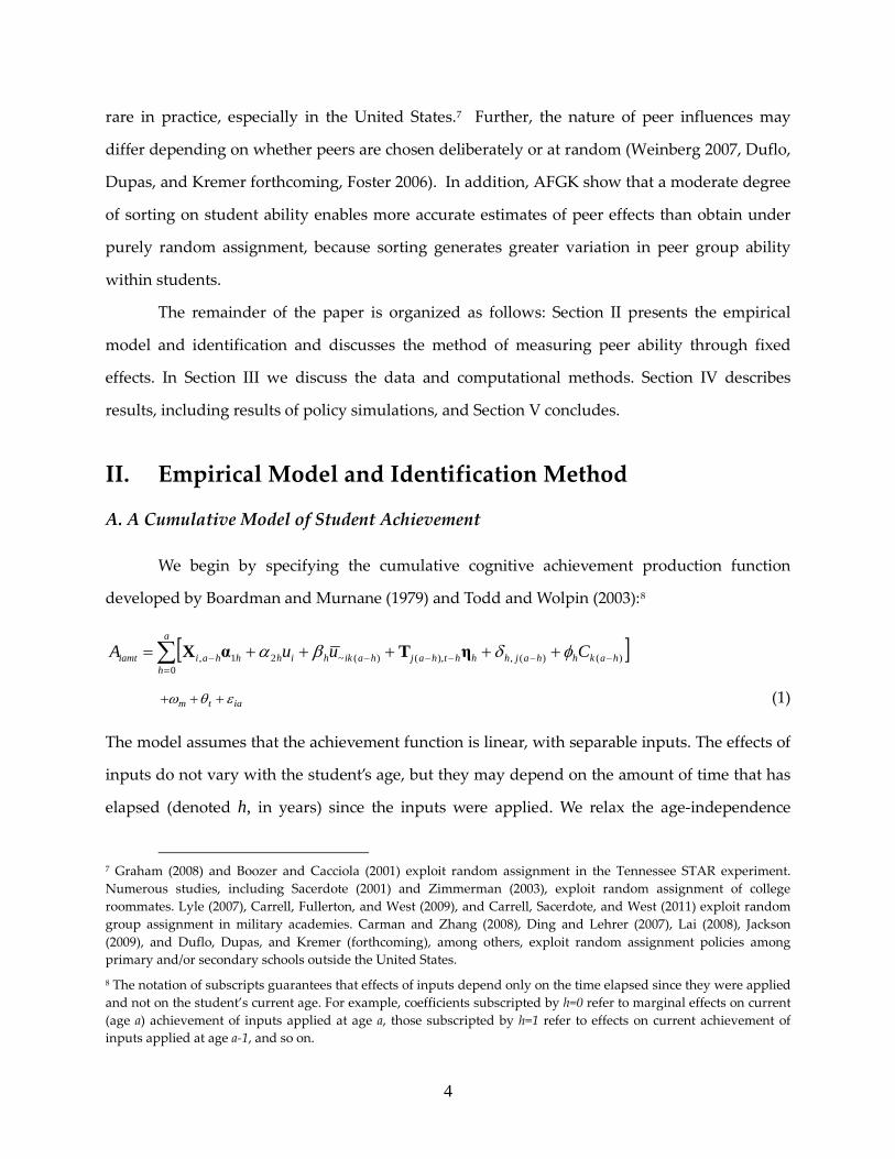
We begin by specifying the cumulative cognitive achievement production function

developed by Boardman and Murnane (1979) and Todd and Wolpin (2003):8

[ ]∑=

−−−−−− +++++=a

hhakhhajhhhthajhaikhihhhaiiamt CuuA

0)()(,),()(~21, φδβα ηTαX

iatm εθω +++ (1) The model assumes that the achievement function is linear, with separable inputs. The effects of

inputs do not vary with the student’s age, but they may depend on the amount of time that has

elapsed (denoted h, in years) since the inputs were applied. We relax the age-independence

7 Graham (2008) and Boozer and Cacciola (2001) exploit random assignment in the Tennessee STAR experiment. Numerous studies, including Sacerdote (2001) and Zimmerman (2003), exploit random assignment of college roommates. Lyle (2007), Carrell, Fullerton, and West (2009), and Carrell, Sacerdote, and West (2011) exploit random group assignment in military academies. Carman and Zhang (2008), Ding and Lehrer (2007), Lai (2008), Jackson (2009), and Duflo, Dupas, and Kremer (forthcoming), among others, exploit random assignment policies among primary and/or secondary schools outside the United States. 8 The notation of subscripts guarantees that effects of inputs depend only on the time elapsed since they were applied and not on the student’s current age. For example, coefficients subscripted by h=0 refer to marginal effects on current (age a) achievement of inputs applied at age a, those subscripted by h=1 refer to effects on current achievement of inputs applied at age a-1, and so on.

5

assumption somewhat by estimating separate models for elementary, middle, and high school

observations.9

Equation (1) relates the current achievement level, Aiamt, for individual i at age a in grade

m in calendar year t, to the entire history of educational inputs applied at each age, from the

current age, a, back to age 0. Inputs include a vector, Xi,a-h, of observed, age-varying

characteristics of individual i; a composite of fixed (observed and unobserved) individual

characteristics, iu , (including the student’s ability endowment and the fixed portion of the flow

of parental inputs);10 the average, )(~ haiku − , of the fixed (composite) characteristics of individual

i's peers (not including herself) in classroom k(a-h) at age a-h;11 a vector of observed (time-

varying) characteristics, Tj(a-h),t-h, such as years of experience, of teacher j(a-h)—the teacher

assigned to the student at age a-h—as of time t-h; the combined impact of the fixed (observed

and unobserved) characteristics of the age a-h classroom teacher, )(, hajh −δ , an effect that

depends on the teacher’s identity and on the time elapsed (h) since she taught the student; and

the class size experienced by the student at age a-h, Ck(a-h). Achievement also depends on the

student’s grade level, m, which contributes the fixed effect mω , and on the calendar year, t,

which contributes the fixed effect tθ . Finally, there is an age-a random disturbance, iaε .12

To facilitate estimation of the model, additional assumptions are necessary. First, we

assume that the impact of the fixed individual characteristics is age-invariant—that is, α2h=α2.

This implies that the net impact on the achievement level of the fixed idiosyncratic inputs is a

constant or fixed effect, which we denote as ii uα2≡γ . In addition, we assume that the marginal

9 A detailed discussion of the derivation of the achievement model is contained in Todd and Wolpin (2003) and Harris, Sass and Semykina (2010). 10 We bundle observed and unobserved characteristics into a single term, because the fixed-effects estimation technique does not allow us to recover the effects of observed fixed characteristics, such as race and gender, separately. The same bundling applies to peers’ fixed characteristics. 11 The specification allows a student’s own time-varying and fixed characteristics to influence her achievement level, but assumes that only the fixed characteristics of peers enter the equation. This is fairly standard in the empirical literature, as most specifications measure peer attributes with fixed or quasi-fixed observable characteristics like lagged test scores, race, gender, disability status, and socio-economic status. 12 Effectively, the model assumes that prior random disturbance terms, as well as prior grade-level and calendar-year effects, have zero persistence.

6

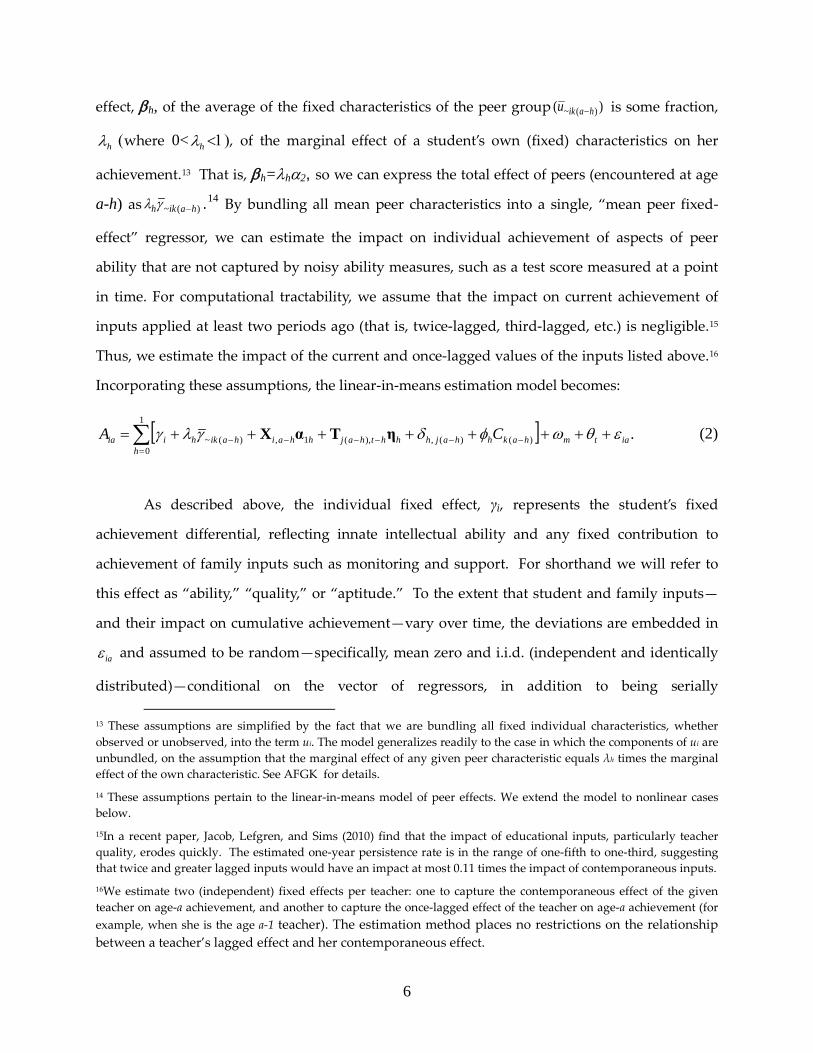
effect, βh, of the average of the fixed characteristics of the peer group )( )(~ haiku − is some fraction,

hλ (where 0< hλ <1), of the marginal effect of a student’s own (fixed) characteristics on her

achievement.13 That is, βh=λhα2, so we can express the total effect of peers (encountered at age

a-h) as )(~ haikh −γλ .14 By bundling all mean peer characteristics into a single, “mean peer fixed-

effect” regressor, we can estimate the impact on individual achievement of aspects of peer

ability that are not captured by noisy ability measures, such as a test score measured at a point

in time. For computational tractability, we assume that the impact on current achievement of

inputs applied at least two periods ago (that is, twice-lagged, third-lagged, etc.) is negligible.15

Thus, we estimate the impact of the current and once-lagged values of the inputs listed above.16

Incorporating these assumptions, the linear-in-means estimation model becomes:

[ ] .1

0)()(,),(1,)(~ iatm

hhakhhajhhhthajhhaihaikhiia CA εθωφδγλγ ++++++++= ∑

=−−−−−− ηTαX (2)

As described above, the individual fixed effect, γi, represents the student’s fixed

achievement differential, reflecting innate intellectual ability and any fixed contribution to

achievement of family inputs such as monitoring and support. For shorthand we will refer to

this effect as “ability,” “quality,” or “aptitude.” To the extent that student and family inputs—

and their impact on cumulative achievement—vary over time, the deviations are embedded in

iaε and assumed to be random—specifically, mean zero and i.i.d. (independent and identically

distributed)—conditional on the vector of regressors, in addition to being serially

13 These assumptions are simplified by the fact that we are bundling all fixed individual characteristics, whether observed or unobserved, into the term ui. The model generalizes readily to the case in which the components of ui are unbundled, on the assumption that the marginal effect of any given peer characteristic equals λh times the marginal effect of the own characteristic. See AFGK for details. 14 These assumptions pertain to the linear-in-means model of peer effects. We extend the model to nonlinear cases below. 15In a recent paper, Jacob, Lefgren, and Sims (2010) find that the impact of educational inputs, particularly teacher quality, erodes quickly. The estimated one-year persistence rate is in the range of one-fifth to one-third, suggesting that twice and greater lagged inputs would have an impact at most 0.11 times the impact of contemporaneous inputs. 16We estimate two (independent) fixed effects per teacher: one to capture the contemporaneous effect of the given teacher on age-a achievement, and another to capture the once-lagged effect of the teacher on age-a achievement (for example, when she is the age a-1 teacher). The estimation method places no restrictions on the relationship between a teacher’s lagged effect and her contemporaneous effect.

7

uncorrelated.17 However, because we estimate separate models for each of elementary school,

middle school, and high school outcomes, we effectively allow for systematic variation in the

contributions of unobserved student-level inputs across schooling levels, as well as variation in

the strength of peer effects.

While we assume that student-level inputs contribute a fixed effect to the achievement

level, Todd and Wolpin (2007) find evidence that family inputs contribute a constant gain effect

on achievement. If there were indeed individual heterogeneity in achievement gains, then the

divergence between high-achieving and low-achieving students should increase with age.

However, in an analysis of the Florida data (results available in the appendix), we observe little

systematic variation in gains with the initial achievement level. In fact, we find evidence that

students initially in the lower tail of the distribution exhibit above-average subsequent gains,

while those in the upper tail exhibit below-average gains.

For illustrative purposes, we have described a model in which peer effects operate

linearly through average peer ability. It seems reasonable to expect that students might benefit

more from high-aptitude peers than from low-aptitude peers (that is, effects are monotonic in

peer ability), for example if high-aptitude peers ask penetrating questions and provide key

insights during classroom discussions more frequently than do lower-aptitude students.

However, it is not obvious that such benefits would be linear in peer ability, nor that such

benefits would accrue uniformly to all types of students, and even the monotonicity property is

an empirical question. Indeed, a growing list of papers finds evidence of nonlinearities in peer

effects (see footnotes 1 and 6 above for examples of such papers). Such findings constitute an

important development, because policy can hope to generate aggregate achievement gains only

if peer effects are nonlinear and therefore non-zero-sum in their impact on achievement.

Accordingly, we estimate two nonlinear models of peer effects. In the first, the influence

of the mean peer fixed effect is allowed to depend on a quintile ranking of the student’s initial

achievement level (based on an initial test score) relative to the entire population of students in

17Evidence of systematic responses in parental inputs to changes in schooling inputs reveal mixed results. See, for example, Bonesr∅nning (2004) and Houtenville and Conway (2008).

8

Florida.18 In the second, peer effects again depend on the student’s initial test-score rank, but the

measure of peer quality is no longer the mean peer fixed effect. Instead, similar to the model of

Carrell, Sacerdote, and West (2011), students are influenced by the respective shares of peers in

the bottom quintile and top quintile of the global distribution of student fixed effects, and in

turn these effects depend on the student’s initial test-score ranking. The share of peers in the

middle of the distribution is omitted due to collinearity.

B. Identification of peer effects

The identification of peer effects at the classroom level poses some daunting challenges.

Manski (1993) first articulated the essential identification problems for peer effects estimation.

These include the reflection problem (or simultaneity), in which spillover effects from peers’

characteristics (such as gender or scholastic aptitude) cannot be identified separately from

spillover effects of peers’ endogenous outcomes (such as test scores). The reflection problem

also hinders identification of the effects of own characteristics on outcomes. A related problem

concerns correlated effects, or common unobserved factors within a peer group (such as teacher

quality) that may produce spurious correlations in peer outcomes. These identification issues

are pertinent regardless of whether peers are randomly assigned or not. However, non-random

assignment adds considerably to the difficulty of surmounting them and, therefore, constitutes

a central concern in the empirical literature (Epple and Romano 2011).

B.1 Non-random assignment and correlated effects

The main identification challenge we face emanates from potential non-random

assignment of students to schools, classrooms, and teachers on the basis of unobserved factors.

As explained by Moffitt (2001), non-random assignment produces correlated effects—in this case,

common unobserved factors influencing achievement within a peer group—which may bias

peer effects estimation. To meet this challenge, we estimate a model that controls for

unobserved heterogeneity in achievement contributions at multiple levels: the individual

18 In the elementary school estimation we use the first available test score, the third grade national percentile ranking. For middle school we use the last elementary school score (fifth grade), and for high school we use the last middle school score (eighth grade).

9

student, the teacher-school pair (and lagged teacher-school pair), the grade level, and the

calendar year. The model controls for numerous time-varying observed factors as well, such as

the teacher’s years of experience, class size, and whether the student is repeating the given

grade. This method isolates quasi-experimental variation in the distribution of peer group

ability (summarized by the mean or possibly other moments) within a student over time (within

each schooling level) that is independent of the various controls.

The inclusion of controls for unobserved teacher inputs, while simultaneously

controlling for student fixed effects, marks a significant methodological contribution, as we

know of no previous study of classroom peer effects that controls for both of these levels of

effects in the same model. The added level of control is important in light of research showing

that teacher quality matters a great deal for student achievement and yet is not strongly linked

to observed teacher characteristics (see, for example, Rockoff 2004, Rivkin et al. 2005, and Kane,

Rockoff, and Staiger 2008). Furthermore, there is abundant evidence that teacher assignments

are non-random within schools (Oakes et al. 1990, Argys, Rees, and Brewer 1996, Vigdor and

Nechyba 2007, Feng 2009, Clotfelter, Ladd, and Vigdor 2006).

While student fixed effects control for average teacher quality by student (and average

peer group quality), teacher quality may co-vary with peer ability within a student over time.

This will occur, for example, if higher ability students are matched with higher quality teachers

on average and yet there is some randomness in teacher assignments. If so, mean peer ability

will be positively correlated with contemporaneous teacher quality, even after conditioning on

individual ability, and measured peer effects will be biased upward when teacher quality is not

accounted for. Negative matching between teacher and student ability is also a possibility.

Despite our extensive controls, we cannot control for all possible correlated effects at the

classroom level. Common physical inputs, such as computers, desks, and lighting, are not likely

to vary significantly across classrooms within schools, and thus our school fixed effects should

capture these factors.19 Localized shocks are also possible—such as a classroom-specific

19 We control for school fixed effects indirectly, through the use of teacher-school “spell” effects, which capture the fixed effect of each teacher-school pair observed in the data. The reason for adopting this approach, which follows that of Andrews, Schank, and Upward (2004), is discussed in Section III.C below.

10

outbreak of influenza—but will lead to biased estimation only if they are correlated with the

peer variables.

The success of our fixed-effects approach also depends on certain features of the data.

First, there must be sufficient within-student variation in peer-group composition in order to

identify peer effects. Second, this variation must not be collinear with the within-student

variation in the quality of the teacher-school pair. Identification would not obtain, for example,

if schools practiced strict classroom tracking and experienced no in-migration or out-migration.

We eliminate this latter concern by limiting our sample to observations in which all teacher-

school pairs are connected in one large stratum by students moving across teachers and

schools.20 Furthermore, analysis of selection into classrooms on the basis of peer ability and

teacher ability, discussed below and in the appendix, indicates that sufficient variation exists

within our data to identify peer effects.

A second caveat is that fixed effects only alleviate bias associated with sorting on time-

invariant student and teacher characteristics (that is, “static” tracking). As Rothstein (2010)

argues, if students are assigned to teachers on the basis of prior, unobserved shocks to

achievement (“dynamic” tracking) and these shocks are serially correlated, then models with

student and teacher fixed effects will yield biased estimates of teacher quality. For example, if

students who have an unusually high test score in one year are systematically assigned to high-

quality teachers the following year and then in that year fall back towards their typical

achievement level (a case of mean reversion), estimates of teacher effects on student learning

will be biased downward.

Using data from a cohort of students in North Carolina, Rothstein conducts falsification

tests that support the existence of dynamic tracking. He shows that future teachers have

spurious effects on current achievement gains, even when controlling for student fixed effects.

By an analogous argument, estimates of peer effects may also be biased in the presence of

dynamic tracking—for example, if a good shock last period results in a particularly strong peer

group in the current period and the student’s achievement also mean-reverts.

20 To detect strata we employ the grouping algorithm proposed by Abowd, Creecy, and Kramarz (2002) and incorporated into the Stata program felsdvreg.

11

The issue of bias associated with dynamic tracking is unlikely to be a major concern in

our case for a number of reasons. First, Koedel and Betts (2011) show that if dynamic sorting is

transitory, then associated bias will be mitigated by observing teachers over multiple time

periods and controlling for student fixed effects. In keeping with these findings, we employ

student fixed effects and restrict our analysis to teachers who taught at least two classes of

students during the sample period. To provide additional insurance against dynamic-tracking

bias, following Harris and Sass (2011), we further limit our analysis sample to those districts in

Florida in which a Rothstein-style test fails to reject the null of strict exogeneity at a 95 percent

confidence level.21

B.2 Simultaneity, or the reflection problem

Concerning the problem of simultaneity, we adopt a model of cognitive achievement in

which peers influence one another’s outcomes (standardized test score) only through their

(fixed) ability or aptitude and not also through their test scores or variable effort. If valid, this

assumption sidesteps the problem of separately identifying exogenous and endogenous

spillovers. With very few exceptions (such as Cooley 2010 and Kinsler 2009), previous studies of

peer effects in education have not attempted to separate these types of effects, and in most cases

it has been assumed that only exogenous effects were at work.

However, we cannot rule out the possibility of endogenous peer effects. Cooley (2009),

for example, finds evidence of effort spillovers among students, and, as mentioned above, there

is considerable evidence that “bad behavior” among peers can negatively impact achievement.

Our estimates of peer effects should therefore be viewed as reduced-form coefficients that

comprise both direct spillovers from peer ability and any spillovers from consistent behavior

patterns that are predicted by peer ability.

B.3 Measurement error in peer ability

21 We implement the Rothstein test using the methodology of Koedel and Betts (2011). The test checks for significant effects of future teachers on current achievement levels—a violation of the null hypothesis of no relationship—through either teachers’ observed characteristics or teacher fixed effects. This test should not be subject to the bias, identified by Kinsler (2011), that may arise under Rothstein’s (2010) own version of the test. In appendix Table A1, we show that model estimates are very similar between the restricted and unrestricted samples.

12

Most existing studies measure peer ability on the basis of lagged test scores or various

instruments for (current or lagged) test scores, or on the basis of various observable,

predetermined characteristics.22 Such measures may capture true peer ability with considerable

error, resulting in a downward bias on estimated peer effects. By contrast, we measure peer

ability based on the peers’ fixed effects. This measure of peer ability captures the contribution of

both observed and unobserved factors to the student’s achievement level, and thus is designed

to mitigate the measurement error bias associated with measures based on observed factors

only.

This method holds the major computational advantage of facilitating estimation of

multiple levels of fixed effects using a numerical algorithm that approximates nonlinear least-

squares estimation, where the least-squares estimators of the peer effects are consistent in

principle. In addition, it mitigates the risk of bias caused by regression to the mean, a bias that

may affect peer effects estimates based on lagged peer test scores, as explained in Betts and Zau

(2004).

One potential disadvantage of the method is that our results cannot tell us whether

specific peer characteristics (such as race and gender) matter, because these are bundled into the

peer fixed effects together with unobservable inputs. However, recent evidence (Hoxby and

Weingarth 2006 and Cooley 2010) suggests that race and gender effects serve mainly as proxies

for ability, indicating that policy should focus on finding the optimal ability mix rather than the

optimal racial mix.

III. Data, Sample Selection, and Computational Issues

A. Data

In the present study we make use of a unique panel data set of school administrative

records from Florida.23 The data cover six school years, 1999–2000 through 2004–2005, and

22Lavy, Paserman, and Schlosser (2008) use grade repetition as a proxy for ability, and Neidell and Waldfogel (2010) use attendance in pre-school. 23 A more detailed description of the data is provided in Sass (2006).

13

include all public-school students in the state of Florida. Achievement test scores (administered

in March) are available for both math and reading in each of grades 3 through 10, for each of

two different achievement tests. One of these tests is the “Sunshine State Standards” Florida

Comprehensive Achievement Test (FCAT-SSS), a criterion-based exam designed to test the

skills that students are expected to master at each grade level. The FCAT-SSS is a “high-stakes”

test that is used for school and student accountability. The other test is the FCAT Norm-

Referenced Test (FCAT-NRT), a version of the Stanford-9 achievement test used throughout the

country. The FCAT-NRT does not enter into any accountability metrics and is thus a “low-

stakes” test. We use the FCAT-NRT scores because these are available for one additional year

and since, coming from a “low-stakes” test, they are not subject to potential bias from “teaching

to the test.” Although the FCAT-NRT scores are “vertically scaled,” meaning a one-point

difference in the scaled score should represent an equivalent achievement difference beginning

from anywhere on the scale, we norm the scores by grade and year in order to reduce the noise

in our achievement measure. The reduction in noise facilitates convergence of the estimation

procedure, as discussed further below.

B. Sample Selection

To permit a flexible education production function, we divide the sample into three

groups: (1) elementary school observations, used to estimate the model for the 4th and 5th grades;

(2) middle school data, used to estimate the model for the 6th, 7th, and 8th grades; and (3) high

school data, used to estimate the model for the 9th and 10th grades.24 The drawback of estimating

separate models is that we limit the number of observations per student to two in the cases of

elementary and high school, and to three per student for middle school. In a small number of

cases, students are observed more than twice (or, for middle school, more than three times)

because they repeated a grade one or more times.25 Within each level of schooling, we observe

24While 3rd grade test scores are available, they must be excluded from the nonlinear models, as explained below, and so are excluded from all models for data consistency. 25Our estimation models include repeater-by-grade indicators to allow for differential achievement of students who repeat a grade.

14

five cohorts, covering the five academic years beginning with 2000/01 and ending with 2004/05.

Descriptive statistics within each schooling-level sample are given in Table 1.

In the regression analysis, we omit students with only a single test score observation for

a given schooling level because peer effects are not identified for these students. However, we

must also omit these “singletons” from the peer groups of others, because the fixed effects of

singletons are also not identified. If peer influence does not depend on singleton status, and if

singletons are broadly representative of the ability distribution, these biases should not be a

source of concern.

In addition to linking students and teachers to specific classrooms, our data indicate the

(average) proportion of time each student spends in each classroom. We restrict our analysis to

students who receive instruction in the relevant subject area (math or reading/language arts) in

just a single classroom. This exclusion allows us to avoid the problem of determining the proper

math or reading peer group, and the proper teacher, for students with unconventional

schedules. To avoid atypical classroom settings and jointly taught classes, we consider only

courses with 10–40 students and with only one “primary instructor” of record. Finally, we

eliminate charter schools from the analysis, since they may have different curricular emphases,

and because student-peer and student-teacher interactions may differ in fundamental ways

from those in traditional public schools. Details on these sample restrictions and their effects on

the size of the estimation sample are discussed in the appendix.

Previous work has shown that student performance suffers in the first year following a

move to a new school (see, for example, Bifulco and Ladd 2006 and Sass 2006). In light of this

evidence, we include three measures of student mobility among the set of regressors: the

number of schools attended in the current year and indicators of “structural” and

“nonstructural” moves by the student. A structural move is defined as a move in which at least

30 percent of a student’s cohort in the same grade at the initial school makes the same move.

This variable captures the effects of normal transitions from elementary to middle school and

from middle to high school, as well as the impact of significant school re-zonings.

Correspondingly, a nonstructural move is defined as any change in school attendance between

the end of the preceding school year and the current school year that does not satisfy the

15

structural-move condition. This variable captures the impact of moves due to events such as

family relocations and parents exercising school choice options.

Time-varying teacher attributes are captured by a set of four dummy variables

representing varying experience levels: 0 years of experience (first-year teachers), 1 to 2 years of

experience, 3 to 4 years of experience, and 5 to 9 years of experience. Teachers with 10 or more

years of experience are the omitted category.26 In addition to the time-varying teacher and

student factors, all of the remaining regressors represent fixed effects, which are estimated

directly using our iterative method.

C. Empirical estimation method

From Section II, recall the linear-in-means version of the cognitive achievement

production function that we wish to estimate:

[ ] .1

0)()(,),(1,)(~ iatm

hhakhhajlhhhthajhhaihaikhiia CT εθωφδγλγ ++++++++= ∑

=−−−−−− ηTαX (3)

In the equation above, we have substituted Tia, the standardized test score (in either

mathematics or language arts), for Aia, the true achievement level, and the disturbance εia now

embeds measurement error imposed by the test instrument with respect to the true

achievement level. We now denote teacher fixed effects as teacher-school spell effects, )(, hajlh −δ ,

which refers to the effect on the age a test score of having experienced teacher j at school l at

age a-h. The teacher-school “spell” fixed effect allows the combined effect of the teacher-school

pair to be non-additive—for example, some teachers may make more efficient use of a school’s

resources than others, and the same teacher may perform differently at different schools. As

explicated in Andrews, Schank, and Upward (2006), the method does not separately identify

school and teacher contributions to achievement.

26 Most longitudinal studies of student achievement find that the marginal effect of additional teacher experience approaches zero after five years of experience. See, for example, Rockoff (2004), Rivkin et al. (2005), Kane, Rockoff, and Staiger. (2008).

16

AFGK describe a similar achievement function, in which achievement spillovers

likewise operate through peers’ fixed effects. These authors show that, provided certain

assumptions hold, the (nonlinear) least-squares estimators of the peer effect coefficients, hλ̂ , are

consistent for a finite number of observations per student. Under the same set of assumptions

as given in AFGK it can be shown that the consistency results apply to our linear-in-means

model above and also extend to the models of nonlinear peer effects described below.27

However, analytical estimation of the achievement function is computationally difficult,

given the large number of fixed effects operating at multiple levels of aggregation and the

nonlinearity of the least-squares problem. Combining teacher and school effects into teacher-

school spell effects simplifies the estimation considerably, but even with this simplification we

must estimate fixed effects for over 200,000 students, plus two or three grade levels and five

calendar years within each schooling-level model. Standard fixed-effects methods eliminate one

level of effects by de-meaning the data with respect to the variable of interest, but such a

strategy (for example, de-meaning by student) is not only insufficient in our case, it is not

feasible when estimating spillovers from peers’ fixed effects.

To estimate the model, we adopt an approximate version of the iterative estimation

procedure proposed by AFGK, which we describe in detail in the appendix. AFGK show that

their procedure yields coefficient estimates that converge to the (consistent) nonlinear least-

squares estimators under relatively nonrestrictive assumptions.28 Unfortunately, this estimation

procedure fails to converge when applied to the Florida education data, a problem we attribute

(based on evidence from simulations) to a combination of noise in test scores and relatively few

observations per student. In our approximate version of the procedure, which facilitates

convergence, estimates of current peer effects will be biased downward in expectation relative

27 As discussed in the appendix, including both current and lagged peer effects can be seen as a special case of the heterogeneous peer effects model of AFGK. Current and lagged teacher-school effects are instances of correlated effects, which are also readily incorporated into the estimation framework. Our nonlinear models also represent special cases of heterogeneous peer effects. 28 The estimates of the fixed effects themselves under the iterative procedure also converge to the least-squares solution and yet these estimates are not consistent.

17

to the true least-squares estimators. The downward bias constitutes an attenuation effect, since

in our approximate method the individual fixed effects are measured with error.

We show through simulations, described in the appendix, that the downward bias is

likely to be small to moderate given the conditions present in our data. In particular, our

approximate method produces estimates in which the downward bias on current peer effects

varies from 4 percent to 19 percent under simulated data conditions that mirror those in the

Florida data.29 Simulations indicate, further, that our results should be fairly robust to noise. As

discussed in the appendix, the downward bias on current peer effects is likely to be relatively

weak in the results for reading at the middle school and high school levels and stronger for

mathematics in middle school and high school; elementary school results (whether for math or

reading) constitute the intermediate case.

IV. Results

A. Mean Peer Effects

We first discuss results under linear-in-means specifications. In these models, we

estimate the effects on current achievement of the average ability (as measured by our fixed

effects) of current classroom peers as well as once-lagged classroom peers (not including the

student herself in the peer means).30 Table 2 reports coefficient estimates for the covariates of

interest under our preferred model specification, in which we account for multiple levels of

fixed effects, including teacher-school spell effects.

We find positive and highly significant effects of current peer ability within every level

of schooling and subject, with the exception of middle school math. These effects are quite small

in magnitude, however. For elementary school mathematics—the largest estimated effect—an

increase in current peer ability from the population mean to 0.25 standard deviations above the

29The relevant data conditions concern the degree of sorting into classrooms by student ability and the degree of matching between student ability and teacher ability. These issues are discussed in detail in the appendix. 30For comparison, we also estimate models in which the peer group—whether current or lagged—consists of all others in the same grade level and school in a given year. Unless specified otherwise, results pertain to classroom peer effects.

18

mean (about 10 percentile points) would yield an increase in own achievement of 0.007

standard deviation units or about one-quarter of a percentile point. For comparison, this effect

is equal to the gain (also in elementary math) from reducing class size by three students, and

amounts to about half the gain from having a teacher with 1-to-2 years of experience rather than

a novice teacher. For both math and reading, current peer effects are substantially larger at the

elementary school level than at the middle or high school level. These results are consistent with

the fact that elementary school students typically spend the entire school day with the same

peer group, whereas middle and high school students experience multiple peer groups during

the typical six-period or seven-period school day.

As expected, in all but one case, the coefficient on lagged peer ability is smaller than that

on current peer ability. In all cases except high school reading, lagged peer effects are at least

marginally significant (10 percent level or better), evidence that peers have persistent effects on

achievement levels. While the presence of some negative lagged peer effects may appear

puzzling, the sizes of the negative effects are trivial, an order of magnitude smaller than the

contemporaneous peer effects. Further, results from nonlinear models (discussed below)

suggest negative peer influences need not be perverse.

Notice that the signs on most of the time-varying regressors are as we would expect:

achievement declines with number of schools attended in a year, for all grades and subjects.

Larger class size has a uniformly negative impact on outcomes. The class size effects are

significant for all grade levels in the case of math, and for elementary school only in the case of

reading. Notice also that within-teacher variation in years of experience has fairly small effects

on achievement, with most of the gain coming in the early years, consistent with findings of

Rivkin, et al. (2005) and Harris and Sass (2011).

Table 3 gives results for a model that is similar to that reported in Table 2, but where

student observations from elementary and middle school are pooled. With this pooling, we can

restrict the minimum observations per student to three rather than two in order to reduce noise

in estimates of student fixed effects and assess robustness of results to this refinement. The

tradeoff is that coefficients can no longer vary between elementary and middle school. As

expected, the estimated current peer effects are roughly intermediate between the elementary-

19

only and middle school-only estimates. For math achievement, the current peer effect becomes

very small and statistically insignificant. For reading, the current peer effect is positive and

statistically significant. Within-year student moves have a negative effect on student

performance in both subjects, and class size continues to be negatively correlated with math

achievement. The point estimates on specific levels of teacher experience vary from those in the

disaggregated models, but payoffs to experience remain relatively small and occur mainly in

the first years of teaching.

Table 4 shows how different model specifications influence the current peer effect

estimates.31 The coefficients in the first row correspond to those from our preferred

specification, reported in Table 2. The coefficients in the second row come from a model in

which we do not control for unobserved teacher effects—we use school fixed effects rather than

teacher-school spell effects. In the third row, the peer group is defined as all others in the same

grade level (within the same school and year), but the specification is otherwise identical to the

preferred one.

Observe first that estimated peer effects are generally larger in the absence of teacher

fixed effects. At the elementary level, the (current) peer effect in math without teacher controls,

at 0.0635, is more than double the estimated effect with the controls. Similarly, in elementary

reading the peer coefficient increases by more than 50 percent in the absence of teacher controls.

This coefficient difference is at least marginally significant in all cases except high school

reading and high school math. On the whole, the results suggest a positive correlation between

average current peer ability and teacher quality—current and/or lagged—controlling for

individual ability. This correlation produces an upward bias on estimated peer effects when

teacher fixed effects are omitted.

The second important finding is that positive peer effects largely disappear when peer

influences are measured at the (within school) grade level. Estimated grade-level peer effects

are statistically insignificant at all schooling levels in math and in elementary school reading.

The only case in which there is a positive and even marginally significant effect is for high

31Unless otherwise specified, all models reported in this table include the same set of controls as the baseline model presented in Table 2.

20

school math. Taking these results at face value, a natural interpretation is that the classroom

setting facilitates learning spillovers in a way that nonclassroom interactions do not. Taking a

skeptical view, we are also more likely to obtain spurious peer effects at the classroom level

than at the grade level due to endogenous classroom assignment and/or classroom-wide

unobserved shocks, despite our efforts to avoid such pitfalls.

B. Nonlinear Peer Effects

As a first step in relaxing the linear-in-means specification, we allow the impact of mean

peer ability to depend on the student’s own “type,” where type is simply an indicator of

baseline achievement within the schooling level. In particular, we take the national percentile

rank of the student’s initial score on the FCAT-NRT test—in the grade preceding the estimation

sample—and place it within the distribution of these ranks among her Florida public-school

cohort (defined by grade level and year).32 The student is a “low” type if her initial percentile

rank falls in the bottom quintile of the Florida distribution, a “middle” type if it falls between

the 20th and 80th percentiles, and a “high” type if it lies in the top quintile.33 Results are reported

in Table 5.34

Among elementary school students, middle and high type students gain about equally

(in either subject area) from an improvement in average current peer ability, whereas low type

students are either unaffected (math) or are made worse off by a small margin (reading). The

magnitude of the positive spillovers for middle and high type students is roughly twice the size

of the effect averaged over all students (that is, the estimates in Table 2). In middle and high

school math, all types of students gain from an improvement in average (current) peer quality,

but the gains are two to three times larger for high type students than for middle types. In

32In elementary school, the earliest score observed is for 3rd grade. Because we use 3rd grade scores to define (predetermined) type, we must omit 3rd grade outcomes from the estimation sample. 33While this type indicator is an imperfect measure of ability, identifying heterogeneity in peer effects along an observable dimension has at least two distinct advantages: first, policy recommendations that apply to a given type will be implementable (in principle); second, according to AFGK, types must be based on observed factors in order to guarantee consistency of least-squares estimators of the heterogeneous (type-specific) peer effects. 34Due to the computational costs of estimating the nonlinear models, we estimate only our preferred specification (including teacher effects, no singleton students, classroom-level effects). We assume that the impact of changes in specification would be similar qualitatively to the impact on the results in the linear models.

21

middle school reading we find no significant (current) peer effects. For high school reading,

middle and high types both benefit significantly (and roughly equally) from an improvement in

average current peer ability, while low types are made significantly worse off.

Looking at lagged peer effects in the one-way heterogeneity model, we find that the

negative impact of lagged peers observed, for example, in the case of elementary school math, is

driven by the (negative) impact of lagged mean peer ability on low type students. More in line

with expectations, middling and high types each experience positive spillovers (on elementary

school math scores) from lagged mean peer ability, spillovers that are smaller than the

respective spillovers from current peer ability.

To allow for an even more complex set of peer influences, we estimate a two-way

interaction model, similar to those of Hoxby and Weingarth (2006) and Carrell, Sacerdote, and

West (2011). In this model, the achievement level of each student type (low, middle, and high,

as defined above) is influenced by the (respective) shares of peers in each of three regions of the

sample-wide distribution of individual fixed effects; the bottom quintile, the middle three

quintiles, and the top quintile. To estimate these effects, we construct six peer variables, each

the product of a binary (own) type indicator and the proportion of peers of a given ability rank:

for example, “individual of low type × fraction of peers in lowest ability quintile,” “individual

of low type × fraction of peers in highest quintile,” and similarly for middle and high type

individuals. Due to collinearity of the proportions, we omit the effect of the proportion of

middle ability peers on each individual type. Therefore, the marginal effect (on a given type) of

an increase in the proportion of high-ability peers (alternatively, low-ability peers) represents

the net effect of increasing the high-ability (low-ability) proportion and reducing the middle-

ability proportion, since the low-ability (high-ability) proportion and class size are being held

constant.

Table 6 reports the current peer effect coefficients for each of the six subject-by-schooling

level models. Among the elementary school results, all effects are highly significant and are

consistent across math and reading. For both subjects, we observe considerable heterogeneity in

the nature of effects by own type and segment of peer group. Low type students are made

worse off by increases in the fraction of peers at either extreme of the ability distribution—that

22

is, they reap greater benefits from peers of middling ability than from either high or low-ability

peers. Middle type students are made worse off by an increase in the fraction of low-ability

classmates and better off by an increase in the share of high-ability peers—suggesting that they

rank peers directly in accordance with their ability. High type students benefit from an increase

in the share of peers in the lowest ability quintile, as well as from an increase in the proportion

of high-ability peers.

The magnitudes of these latter peer effects are economically significant. For example,

among high initial-score students (high types) in math, an increase in the proportion of top-

quintile peers from 0.2 to 0.4 is associated with an increase of 0.03 standard deviations in

achievement (1.2 percentiles in the achievement distribution), or about twice the impact of

having a teacher with 1-to-2 years of experience rather being taught by a novice teacher.

At the middle and high school levels current peer effects are qualitatively similar to

those at the elementary level, with an exception in the case of middle school math—middling

types benefit marginally from a higher share of low-ability peers—and with the qualification

that effects are statistically insignificant in a few cases. In most cases, lagged peer effects in the

two-way interaction model have the same sign as the coefficients on the corresponding current

peer variables and yet are smaller in magnitude.

One explanation for heterogeneous peer effects by own type and peer ability could be

that teachers tend to target the instructional level toward the better students in a given class.

When ability differentials in a class are large and teachers target the top students, the weakest

students might feel lost or overwhelmed. When ability differentials within a class are more

moderate, the goals set by the teacher may seem at least within reach of the weaker students,

who may be inspired to do better than if expectations were set very low. In addition, the ability

to learn from peers may depend on students’ relative ability rather than their absolute ability,

since relative ability likely influences the potential for communication and friendship between

peers. While plausible, these arguments cannot explain why high type students appear to

benefit more from low-ability peers than from middling-ability peers.

If initial achievement is a reasonable (if noisy) proxy for ability as measured by fixed

effects, these results can be used to guide policy, although the implications are not clear-cut. For

23

example, middling-ability students would like to be placed with high-ability peers, but high-

ability types prefer other high types (or even low-ability peers) to middling peers. The results

do suggest that some degree of tracking should be preferred to a policy of uniformly mixed

classrooms. For example, dividing students into two tracks—one for below median ability and

another for above median ability, and creating mixed classrooms within each track, would

maximize peer benefits for low-ability students and would allow at least some middling-ability

students to benefit from having peers of higher ability, although high-ability students would

prefer a policy involving stricter segregation by ability. In the schooling experiment in Kenya

described in Duflo, Dupas, and Kremer (forthcoming), a simple two-track policy, enacted in

second grade classrooms in a random sample of schools, was found to have significant benefits

to students across all quantiles of the baseline score distribution.

The effects in our two-way interaction model agree in some respects with the findings of

Hoxby and Weingarth (2006), who estimate a similar model (on elementary and middle school

grades combined), but in which the peer group segments are more finely subdivided. They find,

for example, that low-initial-score students prefer peers of slightly higher ability than

themselves and are made worse off by an increase in the share of peers of very high ability.

They also find that high-scoring students do best when matched with other high-scoring

students. In contrast, using data on Air Force Academy (USAF) students, Carrell, Sacerdote, and

West (2009) find that low-ability students are helped, rather than hurt, by an increase in the

share of high-ability (based on verbal SAT score) peers. This alternative finding for higher

education—in the Air Force Academy in particular—may reflect differences in that institutional

setting compared with primary and secondary education. For example, disparities in ability

among Air Force students are likely to be smaller than those present in our data.

V. Summary and Conclusions

This paper adds to a growing list of studies that use matched panel data to estimate peer

effects in academic achievement. As in earlier studies, the panel data facilitate the identification

of peer effects on academic achievement by enabling control for endogenous variation in peer

24

groups. Unlike many earlier studies, we are able to place students within classroom groups

with specific teachers, and we observe each teacher with more than one group of students.

Accordingly, ours is the first study to control simultaneously for unobserved heterogeneity in

both student ability and teacher effectiveness, among other unobserved effects, and the first to

estimate classroom-level peer effects at the elementary, middle, and high school levels for the

same school system and to compare these to grade-level effects. While not the first to do so, we

add further value by adopting an innovative computational technique that aims both to

facilitate fixed-effects estimation and to minimize measurement error in peer ability, and we

estimate nonlinear peer effects models that allow for non-zero-sum policy implications.

We observe many instances of significant peer effects at the classroom level, but rarely

are effects significant at the general grade level. Such results underscore the importance of

identifying the salient peer group. In addition, estimated peer effects are generally weaker

when we control for unobserved inputs at the teacher-school level. This result indicates that

teacher ability may vary systematically with peer ability, even controlling for individual student

ability, and that it is therefore important to control for teacher effectiveness, ideally through

teacher fixed effects. This finding may also help to account for the fact that we observe smaller

peer effects (comparing linear-in-means models) than have been found in some previous

studies that did not control for teacher effects.

We find that peer effects exhibit subtleties not captured by the linear-in-means

specification. For example, students with low initial achievement levels appear to benefit less,

and may even experience negative effects, from an increase in the average ability of their peer

group than do those with higher initial scores. Our richest model of peer interactions indicates,

further, that these initially weak students prefer to interact with peers in the middle of the

ability distribution rather than to interact with peers in the very top tier. Students with

middling initial achievement levels experience effects that are monotonic in peer ability and

therefore do best when placed with high-ability peers. High achievers prefer high-ability peers

to middling peers, yet they also prefer low-ability peers to middling peers. Thus, monotonicity

is violated for both low and high initial scorers, but most of the evidence supports the single-

25

crossing property, whereby high-ability students benefit more than others from increases in the

share of high-ability peers.

These preferences over peer ability do not point to a single, optimal policy prescription,

since the diverse peer rankings cannot be simultaneously satisfied for all types of students.

However, they do suggest that classroom assignment policies involving some degree of

tracking by ability—such as splitting students into two tracks—should be preferred to policies

in which all classrooms contain a broad mix of students. Taking the single-crossing property

seriously would call for segregating high-ability students in a separate track. However, the

desirability of such a policy—which could increase inequality of outcomes—depends on

whether achievement gains (or losses) are weighted equally regardless of the student’s initial

achievement level, and on whether achievement disparities should matter in addition to

average achievement. If the goal is to raise achievement among the lowest scorers, focus should

be placed on matching such students with others of modestly higher ability rather than with the

top students. While our findings suggest that the distribution of student ability may influence

teaching strategies in ways that benefit some students but not others, more research is needed

to reveal the nature of such strategies and how teacher resources might be best exploited in

light of classroom assignment policies.

26

References Abowd, John M., Robert H. Creecy and Francis Kramarz. 2002. Computing person and firm

effects using linked longitudinal employer-employee data. Technical Paper no. TP-2002-06, U.S. Census Bureau.

Aizer, Anna. 2008. Peer effects and human capital accumulation: The externalities of ADD,

NBER Working Paper no. 14354, National Bureau of Economic Research, Cambridge, MA.

Andrews, Martyn, Thorsten Schank and Richard Upward. 2006. Practical fixed effects

estimation methods for the three-way error components model. Stata Journal 6:461–481. Angrist, Joshua D. and Kevin Lang. 2004. Does school integration generate peer effects?

Evidence from Boston’s Metco program,” American Economic Review 94:1613–1634. Arcidiacono, Peter, Gigi Foster, Natalie Goodpaster and Josh Kinsler. 2010. Estimating

spillovers in the classroom using panel data. Unpublished manuscript. Argys, Laura M., Daniel I. Rees and Dominic J. Brewer. 1996. Detracking America’s schools:

Equity at zero cost? Journal of Policy Analysis and Management 15:623–645. Betts, Julian R. and Andrew Zau. 2004. Peer groups and academic achievement: Panel evidence

from administrative data. Unpublished manuscript, Public Policy Institute of California. Bifulco, Robert and Helen F. Ladd. 2006. The impacts of charter schools on student

achievement: evidence from North Carolina. Education Finance and Policy 1:50–90. Boardman, Anthony E., and Richard J. Murnane. 1979. Using panel data to improve estimates of

the determinants of educational achievement. Sociology of Education 52: 113–121. Bonesr∅nning, Hans. 2004. The determinants of parental effort in education production: Do

parents respond to changes in class size? Economics of Education Review 23:1–9. Boozer, Michael A. and Stephen E. Cacciola. 2001. Inside the ʹblack boxʹ of Project Star:

Estimation of peer effects using experimental data. Yale Economic Growth Center Discussion Paper no. 832.

Carman, Katherine, and Lei Zhang. 2008. Classroom peer effects and academic achievement:

Evidence from a Chinese middle school. Unpublished manuscript.

27

Carrell, Scott E., Richard L. Fullerton, and James E. West. 2009. Does your cohort matter? Measuring peer effects in college achievement. Journal of Labor Economics 27, no. 3:439–464.

Carrell, Scott E. and Mark L. Hoekstra. 2010. Externalities in the classroom: How children

exposed to domestic violence affect everyone’s kids. American Economic Journal: Applied Economics 2, no. 1:211–228.

Carrell, Scott E., Bruce I. Sacerdote, and James E. West. 2011. From Natural Variation to Optimal

Policy? The Lucas Critique Meets Peer Effects. NBER Working Paper no. 02138. Caucutt, Elizabeth. 2002. Educational vouchers when there are peer group effects – size matters.

International Economic Review 43:195–222. Clotfelter, Charles T., Helen F. Ladd and Jacob L. Vigdor. 2006. Teacher-student matching and

the assessment of teacher effectiveness. Journal of Human Resources 41:778–820. Cooley, Jane. 2009. Can achievement, peer effect, estimates inform policy? A view from inside

the black box. University of Wisconsin Working Paper. Cooley, Jane. 2010. Desegregation and the achievement gap: Do diverse peers help? WCER

Working Paper no. 2010-3. Ding, Weili, and Steven F. Lehrer. 2007. Do peers affect student achievement in China’s

secondary schools? Review of Economics and Statistics 89:300–312. Duflo, Esther, Pascaline Dupas, and Michael Kremer. Forthcoming. Peer effects and the impact

of tracking: Evidence from a randomized evaluation in Kenya. American Economic Review.

Epple, Dennis, Elizabeth Newlon and Richard Romano. 2002. Ability tracking, school

competition and the distribution of educational benefits. Journal of Public Economics 83:1–48.

Epple, Dennis, and Richard E. Romano. 1998. Competition between private and public schools,

vouchers, and peer-group effects. American Economic Review 88:33–62. Epple, Dennis, and Richard E. Romano. 2011. Peer effects in education: A survey of the theory

and evidence. In Handbook of Social Economics, vol. 1B, ed. Jess Benhabib, Alberto Basin, and Matthew O. Jackson, 1053–1163. San Diego: Elsevier.

Feng, Li. 2009. Opportunity wages, classroom characteristics, and teacher mobility. Southern

Economic Journal 75, no. 4:1165–1190.

28

Figlio, David N. 2007. Boys named Sue: Disruptive children and their peers. Education Finance

and Policy 2:376–394. Foster, Gigi. 2006. It’s not your peers, it’s your friends: Some progress toward understanding

the educational peer effect mechanism. Journal of Public Economics 90, no. 8–9:1455–1475. Fryer, Roland G. and Paul Torelli. 2010. An empirical analysis of ‘acting white.’ Journal of Public

Economics 94:380–396. Graham, Bryan S. 2008. Identifying social interactions through conditional variance restrictions.

Econometrica 76, no. 3:643–660. Hanushek, Eric A., John F. Kain, and Steven G. Rivkin. 2009. New evidence about Brown v.

Board of Education: The complex effects of school racial composition on achievement. Journal of Labor Economics 27, no. 3:349–383.

Hanushek, Eric A. and Steven G. Rivkin. 2009. Harming the best: How schools affect the black-

white achievement gap. Journal of Policy Analysis and Management 28, no. 3:366–393. Harris, Douglas N. and Tim R. Sass. 2011. Teacher training, teacher quality and student

achievement. Journal of Public Economics 95: 798–812. Harris, Douglas N., Tim R. Sass and Anastasia Semykina. 2010. Value-added models and the

measurement of teacher productivity. Unpublished manuscript. Houtenville, Andrew J. and Karen S. Conway. 2008. Parental effort, school resources and

student achievement. Journal of Human Resources 43, no. 2:437–453. Hoxby, Caroline M. 2000. Peer effects in the classroom: learning from gender and race variation.

NBER Working Paper no. 7867, National Bureau of Economic Research, Cambridge, MA.

Hoxby, Caroline M. and Gretchen Weingarth. 2006. Taking race out of the equation: School

reassignment and the structure of peer effects. Unpublished manuscript.

Imberman, Scott, Adriana D. Kugler, and Bruce Sacerdote. 2009. Katrina’s children: evidence on the structure of peer effects from hurricane evacuees. NBER Working Paper no. 15291, National Bureau of Economic Research, Cambridge, MA.

Jackson, C. Kirabo. 2009. Ability-grouping and academic inequality: Evidence from rule-based

student assignments. NBER Working Paper no. 14911, National Bureau of Economic Research, Cambridge, MA.

29

Jacob, Brian A., Lars Lefgren, and David P. Sims. 2010. The persistence of teacher-induced

learning. Journal of Human Resources 45, no. 4:915–43. Kane, Thomas J., Jonah E. Rockoff and Douglas O. Staiger. 2008. What does certification tell us

about teacher effectiveness? Economics of Education Review 27, no. 6:615–631. Kinsler, Josh. 2009. School Policy and Student Outcomes in Equilibrium: Determining the Price

of Delinquency. Working paper, June 2009. Kinsler, Josh. 2011. Assessing Rothstein’s Critique of Value-Added Models. Working paper,

February 2011. Koedel, Cory and Julian R. Betts. 2011. Does student sorting invalidate value-added models of

teacher effectiveness? An extended analysis of the Rothstein critique. Education Finance and Policy 6, no. 1:18–42.

Kramarz, Francis, Stephen Machin, and Amine Ouazad. 2007. What makes a test score? The

respective contributions of pupils, schools and peers in achievement in English primary education. IZA Discussion Paper no. 3866, Institute for the Study of Labor, Bonn, Germany.

Lai, Fang. 2008. How do classroom peers affect student outcomes? Evidence from a natural

experiment in Beijing’s middle schools. Unpublished manuscript. Lavy, Victor, M. Daniele Paserman, and Analia Schlosser. 2008. Inside the black box of ability

peer effects: Evidence from variation in low achievers in the classroom. NBER Working Paper no. 14415, National Bureau of Economic Research, Cambridge, MA.

Lefgren, Lars. 2004. Educational peer effects and the Chicago Public Schools. Journal of Urban

Economics 56:169–91. Lyle, David S. 2007. Estimating and interpreting peer and role model effects from randomly

assigned social groups at West Point. Review of Economics and Statistics no. 89, 2:289–299. Manski, Charles F. 1993. Identification of endogenous social effects: The reflection problem.

Review of Economic Studies 60:531–542. Moffitt, Robert A. 2001. Policy interventions, low-level equilibria, and social interactions. In

Social Dynamics, ed. Steven N. Durlauf and H. Peyton Young, 45–82. Cambridge MA: MIT Press.

30

Neidell, Matthew and Jane Waldfogel. 2010. Cognitive and non-cognitive peer effects in early education. Review of Economics and Statistics 93, no. 2:562–576.

Oakes, Jeannie, Tor Ormseth, Robert M. Bell, and Patricia Camp. 1990. Multiplying inequalities:

The effects of race, social class, and tracking on opportunities to learn mathematics and science. Thousand Oaks, CA: RAND.

Rivkin, Steven G., Eric A. Hanushek and John F. Kain. 2005. Teachers, schools and academic

achievement. Econometrica 73:417–458. Rockoff, Jonah E. 2004. The impact of individual teachers on student achievement: Evidence

from panel data. American Economic Review 94:247–252. Rothstein, Jesse. 2010. Teacher quality in educational production: Tracking, decay and student

achievement. Quarterly Journal of Economics 125, no. 1:175–214. Sacerdote, Bruce L. 2001. Peer effects with random assignment: Results for Dartmouth

roommates. Quarterly Journal of Economics 116, no. 2:681–704. Sass, Tim R. 2006. Charter schools and student achievement in Florida. Education Finance and

Policy 1:91–122. Todd, Petra E. and Kenneth I. Wolpin. 2003. On the specification and estimation of the

production function for cognitive achievement. Economic Journal 113:F3–F33. Todd, Petra E. and Kenneth I. Wolpin. 2007. The production of cognitive achievement in

children: Home, school and racial test score gaps. Journal of Human Capital 1, no. 1:91–136.

Vigdor, Jacob L. and Thomas S. Nechyba. 2007. Peer effects in North Carolina public schools. In

Schools and the equal opportunity problem ed. P.E. Peterson and L. Wößmann. Cambridge MA: MIT Press.

Weinberg, Bruce. 2007. Social interactions with endogenous associations. NBER Working Paper

no. 13038, National Bureau of Economic Research, Cambridge, MA. Zabel, Jeffrey E. 2008. The impact of peer effects on student outcomes in New York City public

schools. Education Finance and Policy 3:197–249.

Zimmerman, David. 2003. Peer effects in academic outcomes: Evidence from a natural experiment. Review of Economics and Statistics 85, no. 1:9–23.

31

Table 1 Mean Values for Florida Public School Students, 1999/2000–2003/2004

Math Reading Elementary Middle High School Elementary Middle High School (Grades 3–5) (Grades 6–8) (Grades 9–10) (Grades 3-5) (Grades 6–8)(Grades 9–10) - Normed Achievement Level 0.1817 0.0222 0.5944 0.1795 0.4330 0.5998

Std. Dev. of Achiev. Level 0.9323 0.8741 0.9940 0.9290 0.8556 0.8249

Number of Schools Attended 1.0263 1.0276 1.0134 1.0265 1.0199 1.0111

“Structural” Mover 0.0087 0.2299 0.3101 0.0082 0.1976 0.3703

“Nonstructural” Mover 0.0871 0.1165 0.1240 0.0880 0.1024 0.1313

Class Size 25.6410 28.0467 27.8566 25.7417 26.6857 28.0044

Teacher Experience 11.6039 9.3570 11.8577 11.6231 10.5089 11.4237

32

Table 2 Estimates of the Determinants of Math and

Reading Achievement in Florida, 1999/2000–2004/2005

______________________________________________________________________________ Math Reading _________________________________ _________________________________ Elementary Middle High School Elementary Middle High School (Grades 4–5) (Grades 6–8) (Grades 9–10) (Grades 4–5) (Grades 6–8)(Grades 9–10) ______________________________________________________________________________ Mean Peer Fixed Effect 0.0292*** -0.0013 0.0088** 0.0271*** 0.0087* 0.0124*** (0.0029) (0.0026) (0.0037) (0.0021) (0.0048) (0.0044) Mean Lagged Peer -0.0033** 0.0083*** 0.0145*** -0.0031*** -0.0039* 0.0027 Fixed Effect (0.0013) (0.0012) (0.0013) (0.0011) (0.0022) (0.0022) Number of Schools -0.0255** -0.0645*** -0.2955*** -0.0215* -0.0708*** -0.0343** Attended (0.0113) (0.0053) (0.0144) (0.0114) (0.0123) (0.0165) Structural Mover 0.0642* -0.0285*** 0.0405*** 0.0333 -0.0128 -0.1332*** (0.0384) (0.0073) (0.0097) (0.0357) (0.0139) (0.0487) Nonstructural Mover -0.0015 -0.0173*** 0.0465*** -0.0063 -0.0028 -0.0264 (0.0077) (0.0039) (0.0088) (0.0061) (0.0087) (0.0171) Class Size -0.0022*** -0.0014*** -0.0057*** -0.0013** -0.0005 -0.0004 (0.0008) (0.0002) (0.0005) (0.0006) (0.0005) (0.0005) Teacher with 0 Years 0.0499* 0.0535*** 0.0897*** 0.0275 0.0221 0.0478 of Experience (0.0262) (0.0123) (0.0223) (0.0283) (0.0241) (0.0599) Teacher with 1–2 Years 0.0661*** 0.0606*** 0.0796*** 0.0483** 0.0429* 0.0175 of Experience (0.0187) (0.0086) (0.0162) (0.0212) (0.0228) (0.0493) Teacher with 3–4 Years 0.0759*** 0.0451*** 0.0569*** 0.0563*** 0.0268 -0.0035 of Experience (0.0200) (0.0079) (0.0150) (0.0196) (0.0182) (0.0412) Teacher with 5–9 Years 0.0410*** 0.0286*** 0.0214* 0.0425*** 0.0184 -0.0019 of Experience (0.0144) (0.0068) (0.0112) (0.0142) (0.0142) (0.0285) ______________________________________________________________________________ Number of Students 156,526 231,082 160,400 172,770 88,181 93,123 Number of Observations 315,566 542,650 363,901 348,378 212,281 186,452 ______________________________________________________________________________

Models also include year, grade level, and repeater-by-grade indicators as well as lagged student mobility, class size and teacher experience measures. Bootstrapped standard errors are in parentheses. * indicates significance at the .05 level and ** indicates significance at the .01 level in a two-tailed test.

33

Table 3 Estimates of the Determinants of Math and

Reading Achievement in Florida, 1999/2000–2004/2005 (Minimum of 3 Observations per Student)

______________________________________________________________________________ Math Reading _________________________________ _________________________________ Elementary/Middle Elementary/Middle (Grades 4–8) (Grades 4–8) ______________________________________________________________________________ Mean Peer Fixed Effect 0.0014 0.0154** (0.0010) (0.0067) Mean Lagged Peer -0.0041*** -0.0094*** Fixed Effect (0.0014) (0.0029) Number of Schools Attended -0.1366*** -0.0348* (0.0224) (0.0196) Structural Mover -0.0084 -0.0140 (0.0089) (0.0173) Nonstructural Mover 0.0041 -0.0009 (0.0070) (0.0141) Class Size -0.0037*** 0.0004 (0.0008) (0.0006) Teacher with 0 Years of -0.0832*** 0.0474 Experience (0.0315) (0.0378) Teacher with 1–2 Years of -0.0597** 0.0670** Experience (0.0296) (0.0327) Teacher with 3–4 Years of -0.0599** 0.0284 Experience (0.0276) (0.0257) Teacher with 5-9 Years of -0.0437** 0.0119 Experience (0.0211) (0.0206) ______________________________________________________________________________ Number of Students 109,507 38,982 Number of Observations 370,841 133,189 ______________________________________________________________________________

See notes to Table 2.

34

Table 4 Comparison of Estimated Effects of Mean Peer Fixed Effects on Math and Reading

Achievement in Florida From Models with Varying Peer Group Levels and Varying Teacher Controls, 1999/2000–2004/2005

______________________________________________________________________________ Math Reading _________________________________ _________________________________ Peer Group/ Elementary Middle High School Elementary Middle High School Teacher Controls (Grades 4–5) (Grades 6–8) (Grades 9–10) (Grades 4–5) (Grades 6–8)(Grades 9–10) ______________________________________________________________________________ Classroom Peers/ 0.0292*** -0.0013 0.0088** 0.0271*** 0.0087* 0.0124*** With Teacher FE (0.0029) (0.0026) (0.0037) (0.0021) (0.0048) (0.0044) ______________________________________________________________________________ Classroom Peers/ 0.0635*** 0.0126*** 0.0019 0.0424*** 0.0176*** 0.0150*** No Teacher FE (0.0035) (0.0018) (0.0030) (0.0031) (0.0035) (0.0051) ______________________________________________________________________________ Grade Level Peers/ 0.0044 -0.0003 -0.0012 -0.0031 -0.0315** 0.0100* With Teacher FE (0.0111) (0.0062) (0.0054) (0.0143) (0.0131) (0.0054) ______________________________________________________________________________ Number of Students 156,526 231,082 160,400 172,770 88,181 93,123 Number of Observations 315,566 542,650 363,901 348,378 212,281 186,452 ______________________________________________________________________________

See notes to Table 2.

35

Table 5

Estimates of the Effect of Mean Classroom Peer Fixed Effects by Own Initial Test- Score Quintile on Math and Reading Achievement in Florida, 1999/2000–2004/2005

______________________________________________________________________________ Math Reading _________________________________ _________________________________ Elementary Middle High School Elementary Middle High School (Grades 4–5) (Grades 6–8) (Grades 9–10) (Grades 4–5) (Grades 6–8)(Grades 9–10) ______________________________________________________________________________ Lowest Test-Score Quintile × 0.0170 0.0235*** 0.2681*** -0.0223* -0.0021 -0.0613** Mean Peer Fixed Effect (0.0134) (0.0072) (0.0175) (0.0124) (0.0127) (0.0241) Middle Test-Score Quintiles × 0.0670*** 0.0278*** 0.0532*** 0.0462*** -0.0071 0.0352*** Mean Peer Fixed Effect (0.0092) (0.0027) (0.0060) (0.0078) (0.0079) (0.0095) Highest Test-Score Quintile × 0.0640*** 0.0807*** 0.1657*** 0.0384*** 0.0187 0.0377*** Mean Peer Fixed Effect (0.0130) (0.0075) (0.0093) (0.0111) (0.0133) (0.0141) ______________________________________________________________________________ Number of Students 154,397 169,446 158,939 170,565 153,781 92,945 Number of Observations 311,260 413,979 360,814 343,917 59,724 186,066 ______________________________________________________________________________

See notes to Table 2.

36

Table 6 Estimates of the Effects of Peer Ability Quintile by Own Initial Test-Score Quintile

on Math and Reading Achievement in Florida, 1999/2000–2004/2005

______________________________________________________________________________ Math Reading _________________________________ _________________________________ Elementary Middle High School Elementary Middle High School (Grades 4–5) (Grades 6–8) (Grades 9–10) (Grades 4–5) (Grades 6–8)(Grades 9–10) ______________________________________________________________________________ Lowest Quintile × Fraction of -0.2638*** -0.1263*** -0.4089*** -0.2325*** -0.2643*** -0.3156*** Peers in Lowest Quintile (0.0238) (0.0113) (0.0165) (0.0230) (0.0173) (0.0316) Lowest Quintile × Fraction of -0.2398*** -0.2074*** -0.4553*** -0.2759*** -0.3698*** -0.3976*** Peers in Highest Quintile (0.0351) (0.0241) (0.0540) (0.0347) (0.0532) (0.0654) Mid. 3 Quintiles × Fraction of -0.0482** 0.0172** -0.1287*** -0.0434*** -0.0138 -0.0256 Peers in Lowest Quintile (0.0199) (0.0069) (0.0081) (0.0150) (0.0138) (0.0157) Mid. 3 Quintiles × Fraction of 0.1059*** 0.0698*** -0.0210 0.0615*** -0.0011 -0.0338* Peers in Highest Quintile (0.0165) (0.0067) (0.0129) (0.0212) (0.0174) (0.0197) Highest Quintile × Fraction of 0.1487*** 0.1667*** 0.0874*** 0.1144*** 0.2106*** 0.0824*** Peers in Lowest Quintile (0.0340) (0.0242) (0.0240) (0.0290) (0.0319) (0.0253) Highest Quintile × Fraction of 0.1437*** 0.1614*** 0.2346*** 0.0662*** 0.0780*** 0.0133 Peers in Highest Quintile (0.0313) (0.0101) (0.0116) (0.0238) (0.0291) (0.0267) ______________________________________________________________________________ Number of Students 154,397 169,446 158,939 170,565 59,724 92,945 Number of Observations 311,260 413,979 360,814 343,917 153,781 186,066 ______________________________________________________________________________

See notes to Table 2.