classifying gpr images using convolutional neural networks
TRANSCRIPT

CLASSIFYING GPR IMAGES USING CONVOLUTIONAL NEURAL NETWORKS
By
Maha Almaimani
Dr. Dalei Wu Dr. Yu Liang
Associate Professor of Computer Science Professor of Computer Science
Committee Chair Committee Member
Dr. Li Yang
Professor of Computer Science
Committee Member

ii
CLASSIFYING GPR IMAGES USING CONVOLUTIONAL NEURAL NETWORKS
By
Maha Almaimani
A Thesis Submitted to the Faculty of the University of
Tennessee at Chattanooga in Partial Fulfillment
of the Requirements of the Degree of
Master of Science: Computer Science
The University of Tennessee at Chattanooga
Chattanooga, Tennessee
May 2018

iii
ABSTRACT
This thesis focused on classifying GPR cylinders' B-scans according to their depth, size,
material, and the dielectric constant of the underlying medium using four different architectures
of convolutional neural networks. Two CNNs were newly proposed for this study, while the
other two were used by other authors. These CNNs were trained using a couple of adjusted
training options including initial learning rate, learn rate drop factor, and learn rate drop period;
which had a positive impact on a part of the used models, while the option maximum number of
epochs worked good with all of the used models. Results show that the first newly proposed
CNN showed a superior performance due to the use of a deep network with a large amount of
small filters. Using this model, it was found that the best results were carried out when GPR B-
scans were classified according to the cylinders' materials.

iv
DEDICATION
This thesis is dedicated to the souls of my parents, specially my mother who passed away
during my Master's journey. My deepest gratitude to my three kids (Maya, Marya, and Mahir),
and my wonderful husband (Alaaeldin), I would not be here today if not for his encouragement
and support.

v
ACKNOWLEDGEMENTS
I would like to thank Dr. Wu for his guidance and for giving me the chance to work
under his supervision. It has been a great honor for me to work with him. My sincere
appreciation also goes to my family, friends, colleagues, and the staff of the Department of
Computer Science and Engineering at the University of Tennessee at Chattanooga, who shared
my enthusiasm and helped me go through disappointments. I also would like to thank the
members of the committee Dr. Yu Liang, and Dr. Li Yang.

vi
TABLE OF CONTENTS
ABSTRACT ....................................................................................................................... iii
ACKNOWLEDGEMENTS .................................................................................................v
LIST OF ABBREVIATIONS ..............................................................................................x
LIST OF SYMBOLS ......................................................................................................... xi
CHAPTER ...........................................................................................................................1
I. INTRODUCTION .................................................................................................1
1.1 Significance .....................................................................................................1 1.2 Objectives ........................................................................................................2
II. REVIEW OF RELEVANT LITERATURE ..........................................................3
2.1 GPR History ....................................................................................................3
2.2 Related Work ...................................................................................................7
III. METHODOLOGY ..............................................................................................10
3.1 Software Set ...................................................................................................10 3.2 Data Set Configuration ..................................................................................10
3.3 Data Preprocessing ........................................................................................20 3.4 CNN Background ..........................................................................................22
3.5 Proposed System Architectures .....................................................................27 3.6 Proposed CNN Models ..................................................................................28
IV. EXPERIMENTS AND RESULTS......................................................................36
4.1 Using Default Training Options ....................................................................37 4.2 Adjusting the Initial Learning Rate ...............................................................39 4.3 Adjusting the Learn Rate Drop Factor and the Learn Rate Drop Period ......41 4.4 Adjusting the Maximum Number of Epochs .................................................43
V. SUMMARY AND FUTURE WORK .................................................................45
REFERENCES ..................................................................................................................47
VITA ..................................................................................................................................51

vii
LIST OF TABLES
1 History of GPR Research Since 1900 ............................................................................. 6
2 The Relationship Between Frequency Rate and Depth; and the Relationship
Between Frequency Rate and Resolution ................................................................ 12
3 The Number of Outputs for Each Classification Category in the Four Proposed CNN
Models...................................................................................................................... 30
4 The Characteristics of the Proposed CNNs ................................................................... 35
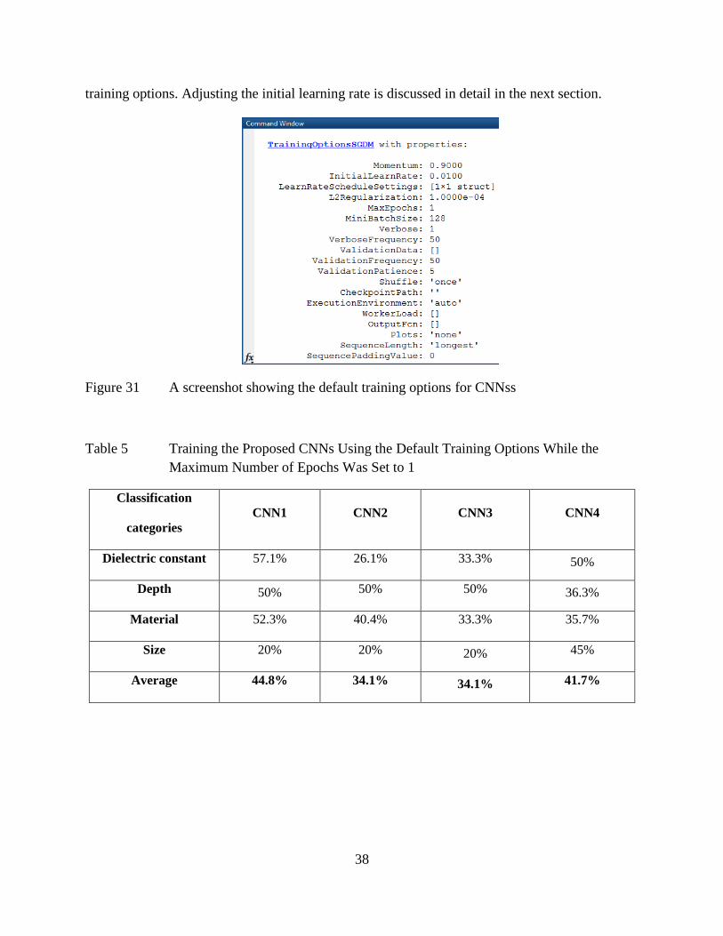
5 Training the Proposed CNNs Using the Default Training Options While the
Maximum Number of Epochs Was Set to 1 ............................................................ 38
6 Training the Proposed CNNs Using the Default Training Options While the
Maximum Number of Epochs Was Set to 100 ........................................................ 39
7 Results After Adjusting the Initial Learning Rate to (0.0001) and Epochs=1 ............... 40
8 Results After Adjusting the Initial Learning Rate to (0.0001) and Epochs=100 ........... 41
9 Epochs=8, and Initial Learning Rate Adjusted to 0.0001 for CNN2 and CNN4 .......... 42
10 Learn Rate Drop Factor=0.5, Learn Rate Drop Period=4, Epochs=8, and Initial
Learning Rate Adjusted to 0.0001 for CNN2 and CNN4 ........................................ 42
11 The Best Combination of the Adjusted Training Options for Each Proposed CNN ..... 43
12 The Needed Number of Epochs for Each Model to Achieve an Accuracy of More
Than 90% Using the Training Options Adjustment Combination in Table 11 ....... 44

viii
LIST OF FIGURES
1 A graphic illustrating the basic principle of GPR ............................................................ 3
2 A graphic showing the relationship between A-scan, B-scan, and C-scan ...................... 4
3 An A-scan of a buried metal cylinder .............................................................................. 4
4 A B-scan of a buried metal cylinder ................................................................................ 5
5 A screenshot showing the license screen for GprMax v3.1.1 ........................................ 11
6 A B-scan generated using a frequency of 1.5e8 ............................................................ 13
7 A B-scan generated using a frequency of 0.5e9 ............................................................ 13
8 A B-scan generated using a frequency of 1.5e9 ............................................................ 14
9 A B-scan generated using a frequency of 3.5e9 ............................................................ 14
10 A screenshot showing an error during a simulation using a high, out-of-range
frequency.................................................................................................................. 15
11 A B-scan generated using a time window of 3e-9 ......................................................... 16
12 A B-scan generated using a time window of 10e-9 ....................................................... 16
13 A B-scan generated using a time window of 20e-9 ....................................................... 17
14 A screen shot of a gprMax script used to create a B-scan of a buried PVC cylinder ........
.................................................................................................................................. 18
15 Geometry of a buried PVC cylinder imaged using Paraview ........................................ 19
16 B-scan of a buried PVC cylinder ................................................................................... 19
17 A screenshot showing HDFView v.3.3.0 ....................................................................... 20
18 Two GPR images showing (L-R) before rescaling; and after rescaling using
HDFView ................................................................................................................. 21
19 Steps of pre-processing GPR images ............................................................................. 22
ix
20 The way CNN models work .......................................................................................... 23
21 Basic CNN architecture ................................................................................................. 23
22 The result after convolving a 5*5 filter.......................................................................... 25
23 Zero padding .................................................................................................................. 25
24 The pooling process ....................................................................................................... 27
25 Proposed system architectures ....................................................................................... 28
26 The first newly proposed CNN model .......................................................................... 30
27 The second newly proposed CNN model ...................................................................... 31
28 The third proposed CNN model ..................................................................................... 33
29 The fourth proposed CNN model .................................................................................. 34
30 The four Proposed CNN models. ................................................................................... 35
31 A screenshot showing the default training options for CNNss ...................................... 38
32 A Screenshot showing a 0% classification accuracy because mini batch loss = NaN ......
.................................................................................................................................. 39

x
LIST OF ABBREVIATIONS
GPR: Ground Penetrating Radar
UXO: Unexploded Ordnance
GP: Genetic Programming
GA: Genetic Algorithm
ANN: Artificial Neural Network
CNN: Convolutional Neural Network
Convnet: Convolutional Neural Network
SGDM: Stochastic Gradient Descent with Momentum

xi
LIST OF SYMBOLS
x: The pixel value
ℓ: The iteration number
α: The learning rate
θ: The parameter vector
E(θ): The loss function
∇E(θ): The gradient of the loss function

1
CHAPTER I
INTRODUCTION
1.1 Significance
Ground penetrating radar (GPR) is a very common non-destructive subsurface imaging
tool used in many applications related to infrastructure evaluations like rebar detection [1],
unexploded ordnance (UXO) detection [2], landmine detection [3], pipeline detection [4],
avalanche victims detection [5] [6], soil moisture assessment [7], liquid contamination detection
[8], soil contamination measurement [9], bridge deck inspection [10], railroad ballast monitoring
[11] [12], etc. Object detection is one objective that was focused on in these applications. Of
equal importance to object detection is buried object characterization or, in other words, finding
the characteristics of the buried object. These characteristics include: object localization, object
depth detection, object shape identification, object size estimation, object dimension estimation,
object material recognition and classification. Currently, not many research projects focus on all
of them. These projects mostly focus on detection. Due to the importance of GPR use in
infrastructure applications, an automatic methodology to find the characteristics of buried targets
in GPR images is very necessary [13]. Thus, an automatic technique is presented in this
document to classify images according to their size, material, depth and the dielectric constant of
the underground medium.

2
1.2 Objectives
The experimental objectives of this project included investigating the effect of different
training options on four convolutional neural networks (convnets, CNNs, convolutional nets) and
finding the best combination of training options for each of the suggested CNNs. In addition,
finding which of these four models would work the best in classifying cylinders' B-scan images
according to their characteristics: depth, material, size, and the dielectric constant of the
underground medium. Finally, examining which of the four classification categories would be
the most accurately classified.
This document includes a total of four chapters beside the introduction. The next chapters
are arranged as follows: Chapter 2 gives a literature review related to the GPR field. Chapter 3
describes the methodology of the project. Chapter 4 is about experiments and results. Finally,
Chapter 5 concludes the thesis and provides a list of future work.

3
CHAPTER II
REVIEW OF RELEVANT LITERATURE
2.1 GPR History
It is necessary to understand the mechanism that lies behind GPR before delving into its
history. GPR works by transmitting electromagnetic waves into the ground. The propagated
waves from the source through the ground hit the buried objects and then are reflected back to
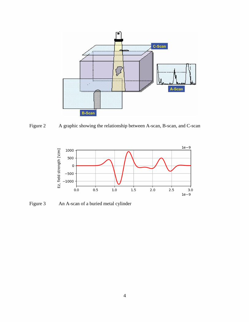
the receiver (Figure 1) [14] to form what so called an A-scan. Different A-scans at different scan
positions are stacked to form a B-scan GPR image. Furthermore, stacked 2D B-scans form what
is known to be a 3D C-scan [15]. These three types of scans are then processed to detect the
buried objects and show their characteristics. The relationship between the three different kinds
of scans is visualized in Figure 2 [16]. Examples of an A-scan and a B-scan are shown in Figure
3 [17] and Figure 4 [17]. B-scans were used in this project, leaving A-scans and C-scans behind
the scope.
Figure 1 A graphic illustrating the basic principle of GPR
4
Figure 2 A graphic showing the relationship between A-scan, B-scan, and C-scan
Figure 3 An A-scan of a buried metal cylinder

5
Figure 4 A B-scan of a buried metal cylinder
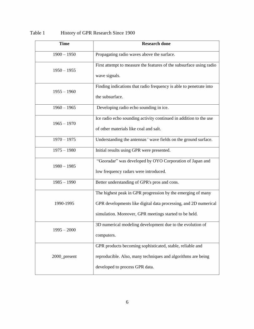
The history of GPR research from 1900 to present is illustrated in Table 1 [18].
6
Table 1 History of GPR Research Since 1900
Time Research done
1900 – 1950 Propagating radio waves above the surface.
1950 – 1955
First attempt to measure the features of the subsurface using radio
wave signals.
1955 – 1960
Finding indications that radio frequency is able to penetrate into
the subsurface.
1960 – 1965 Developing radio echo sounding in ice.
1965 – 1970
Ice radio echo sounding activity continued in addition to the use
of other materials like coal and salt.
1970 – 1975 Understanding the antennas ' wave fields on the ground surface.
1975 – 1980 Initial results using GPR were presented.
1980 – 1985
“Georadar” was developed by OYO Corporation of Japan and
low frequency radars were introduced.
1985 – 1990 Better understanding of GPR's pros and cons.
1990-1995
The highest peak in GPR progression by the emerging of many
GPR developments like digital data processing, and 2D numerical
simulation. Moreover, GPR meetings started to be held.
1995 – 2000
3D numerical modeling development due to the evolution of
computers.
2000_present
GPR products becoming sophisticated, stable, reliable and
reproducible. Also, many techniques and algorithms are being
developed to process GPR data.
7
2.2 Related Work
Many techniques have been deployed to find the characteristics of GPR images. One way
is by using the pattern recognition approach [19]. This approach recognized the materials of the
buried objects automatically, but was not able to recognize their shapes or estimate their sizes.
The use of Genetic Programming (GP) was another method to analyze GPR images.
Genetic programming is an evolutionary learning method that is similar to genetic algorithm
(GA) in its ability to search for the global optimal solution which could minimize efforts on the
training processes. GP is preferred because the size and structure of its solution is unlimited,
while those of the GA solutions are restricted to user-defined constraint. GP was used by [20] to
analyze GPR images and came up with promising results that showed the method's robustness.
However, [20] did not show that this method is reliable by using it in more practical situations
that include multiple targets or various orientations of targets.
A method to classify and recognize features in GPR images based on Support Vector
Machines (SVMs) was also used by many authors. This approach was used by [21] to identify
voids inside concrete and estimate their depth. Results were interesting but the approach needed
to be improved to recognize the shape and the distribution of the voids. SVMs were also used to
identify the material of underground utilities by [22]. This research suggested that in order to get
more accurate classification results using SVMs, the segment length of A-scan should be
adjusted. Furthermore, B-scan information such as feature of amplitude and frequency should be
added to the raw data. Moreover, a proper kernel function and a convenient range for data
normalization should be selected.
Neural networks or Artificial Neural Networks (ANNs) have been used to find buried
objects' characteristics. A paper published in 2016 by [13], exploited three neural networks
8
algorithms to estimate the shape, material, size, and depth of the buried object, as well as the
dielectric constant of the underground medium simultaneously. The proposed neural networks
were able to classify the shape of the buried objects to one of three shapes: circle, triangle, or
square. Furthermore, they could classify the buried objects' material to either: air, limestone, or
metal. Results showed that an error emerged when a metal circular object was being recognized.
Furthermore, triangle size estimation demonstrated that the proposed methodology needed some
improvement to get more accurate results. ANNs were also used by [23] to classify underground
buried object' shape whether it was a cylinder or a cube metal. The problem with neural networks
is that they show limited performance in the case of nonlinear, high dimensional samples. They
are also sensitive to learning samples and they have limited generalization ability according to
[21]. Neural Networks suffer from a group of limitations, therefore, Convolutional Neural
Networks were introduced in this project to overcome the limitations and classify GPR images
more accurately.
Convolutional Neural Networks have revolutionized the field of computer vision and
image classification since 2012. CNNs are deep neural networks where each neuron accepts
inputs from neurons on the previous layer with no existence of cycles, thus they are called feed
forward CNNs [24]. They differ from shallow neural networks that consist of only one layer,
therefore, by using kernels they do not struggle from computational complexity when the input
size is dramatically increased. Shallow models might be effective in solving simple problems but
they will have difficult time dealing with complicated real world applications [25]. Furthermore,
in contrast to other deep neural networks, CNNs work on 2D images directly. They also use the
Back Propagation algorithm which is Gradient Decent. The major task of the Back Propagation
algorithm is to optimize the accuracy of predicting models by reducing the error related to each

9
neuron [26]. Convolutional neural networks have been used in the ground penetrating radar field
by a couple of authors to detect buried targets such as [27], who evaluated the use of CNNs to
classify 2D GPR pictures. CNNs were also exploited in a study conducted by [3] to detect
landmines. Moreover, [28] used the transfer learning technique with CNNs to detect threats. In
neural networks field, transfer learning means a pre-trained neural network model can be used to
solve a new similar problem instead of wasting time and effort training a network from scratch.
The study conducted by [28] used the popular Cifar10 dataset, and a dataset of high resolution
aerial imagery for detecting solar photovoltaic arrays to pre-train their CNN. Until recently,
CNNs were used only to detect objects, without classifying GPR images according to their
characteristics (i.e., depth, size, material, etc.). Therefore, this research deployed Convolutional
Neural Networks to solve this problem.

10
CHAPTER
III. METHODOLOGY
3.1 Software Set
Four software packages were used in this project:
1. GprMax v3.1.1: to generate B-scan images [17].
2. Paraview v4.3: to visualize geometry created by gprMax [29].
3. HDFView v3.0.0: to pre-process the images by rescaling them [30].
4. Matlab R2017b: to do the following:
a. Resize the images.
b. Convert the images to grey scale.
c. Feed the images to the proposed Convolutional Neural Networks' for the sake of
training.
d. Test the CNNS [31].
3.2 Data Set Configuration
There are two types of GPR systems: the stepped frequency systems and the time domain
systems. SF-GPR systems are better than the time domain ones in giving a real reading of the
subsurface structure, but they require a larger measurement time. Therefore, they are not suitable
for extensive public utility searches like pipes, neither for modelling transient phenomena [32].
Therefore, in this research, gprMax, a time domain system was used. GprMax, is an open source
11
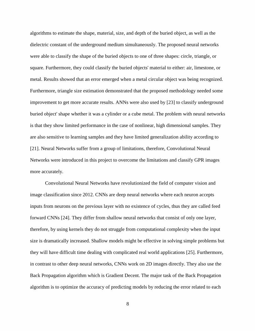
command-line driven software that was written in Python (Figure 5). It uses the Finite-
Difference Time-Domain (FDTD) method to simulate the electromagnetic wave propagation of
Ground Penetrating Radar [17].
Figure 5 A screenshot showing the license screen for GprMax v3.1.1
GprMax has very powerful features such as:
• Built in libraries of antenna models.
• The ability to model realistic subsurface.
• The ability to model realistic objects.
• The ability to build heterogeneous objects.
• The ability to build objects with rough surfaces [17].
GprMax was originally developed in 1996 by Antonis Giannopoulos. Today, three
versions exist and the latest one were used in this research. GprMax can work on both CPU and
GPU, single and multiple. In our experiment, gprMax ran on a single CPU and the GPR

12
waveform was generated as a Ricker waveform.
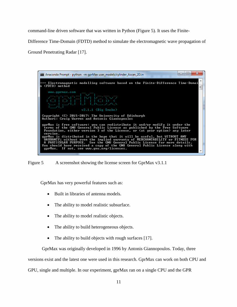
To select the best centre frequency and time window values, a couple of experiments
were conducted. In the case of frequency, the use of high frequency results better resolution and
the use of low frequency results more penetration depth. Table 2 [32] shows the relationship
between frequency rate and depth. It also shows the relationship between frequency rate and
resolution. Different frequencies were applied on a couple of objects with different sizes, depths,
materials, and underlying dielectric constants. Results were as follows: Having a low frequency
did not show good results. Figures 6, 7, 8, and 9 depicts cylinders of the same size, depth,
material, and dielectric constants, but were produced using different frequencies. Figure 6, where
the frequency equalled 1.5e8 shows the worst result. Figures 7 and 8 where the frequencies were
0.5e9 and 1.5e9 respectively show better results, but not the best. Figure 9 shows the best result
with a frequency of 3.5e9. Setting higher and higher frequencies produce better results, but they
take more time to be generated. Worth to notice, each model has a range of frequencies. Using
out of range frequencies (i.e., really high or really low frequencies) generated an error during
simulation. Figure 10 shows an error message because of using an out of range high frequency
(i.e., 4.5e9).
Table 2 The Relationship Between Frequency Rate and Depth; and the Relationship
Between Frequency Rate and Resolution
Frequency Rate Depth Resolution
High frequency shallow high
Low frequency deep low
13
Figure 6 A B-scan generated using a frequency of 1.5e8
Figure 7 A B-scan generated using a frequency of 0.5e9

14
Figure 8 A B-scan generated using a frequency of 1.5e9
Figure 9 A B-scan generated using a frequency of 3.5e9
15
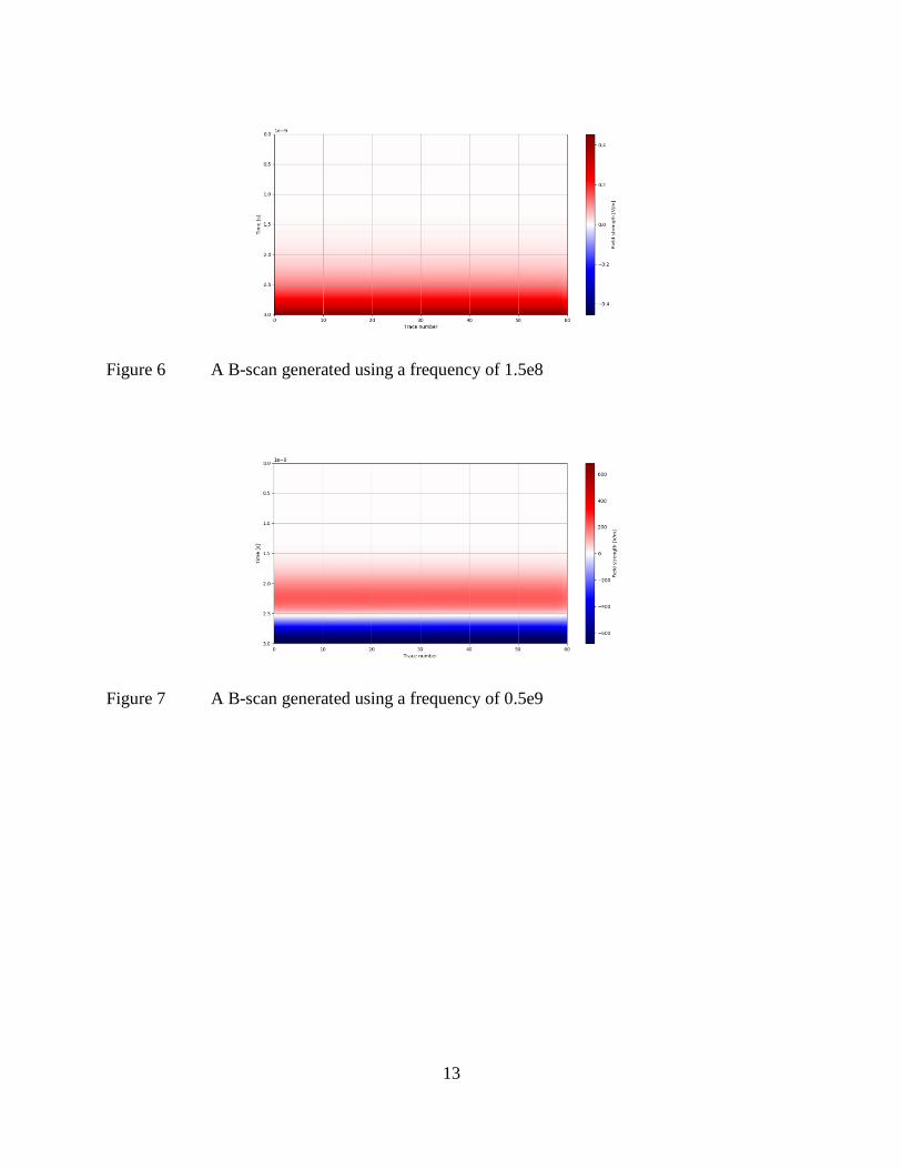
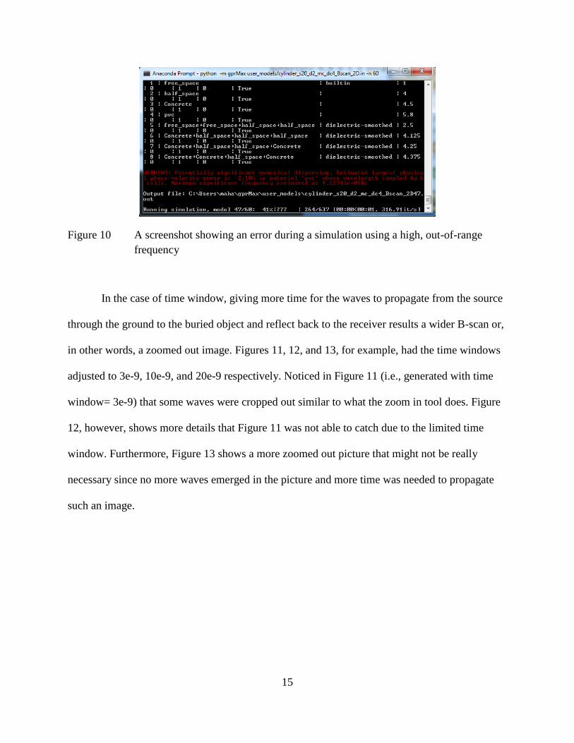
Figure 10 A screenshot showing an error during a simulation using a high, out-of-range
frequency
In the case of time window, giving more time for the waves to propagate from the source
through the ground to the buried object and reflect back to the receiver results a wider B-scan or,
in other words, a zoomed out image. Figures 11, 12, and 13, for example, had the time windows
adjusted to 3e-9, 10e-9, and 20e-9 respectively. Noticed in Figure 11 (i.e., generated with time
window= 3e-9) that some waves were cropped out similar to what the zoom in tool does. Figure
12, however, shows more details that Figure 11 was not able to catch due to the limited time
window. Furthermore, Figure 13 shows a more zoomed out picture that might not be really
necessary since no more waves emerged in the picture and more time was needed to propagate
such an image.

16
Figure 11 A B-scan generated using a time window of 3e-9
Figure 12 A B-scan generated using a time window of 10e-9

17
Figure 13 A B-scan generated using a time window of 20e-9
After conducting many experiments on the centre frequency and the time windows, the
GPR Ricker waveform was set using a centre frequency of 1.5 GHz to get a good resolution with
a reasonable penetration depth. The time window was set to 3 nanoseconds to give enough time
for the waves to propagate from the transmitter and reflect back to the receiver resulting images
with enough details. GPR A-scan traces were collected in a horizontal direction from left to right
using 60 steps on different sized domains. The amplitude of the GPR antenna above the ground
was 1 mm.
Following [13], different geometry models buried in a half-space with different scenarios,
were created using the FDTD simulation, including the following:
• Object shape: cylinder.
• Object Material: metal, concrete, polyvinyl chloride (i.e., PVC).
• Object depth: 2 cm, 100 cm.
• Object size/radius: 20 mm, 50 mm, 100 mm, 150 mm, 200 mm.
• Dielectric constant of the subsurface medium: 4, 6, 8.

18
Figure 14 shows gprMax script to create a B-scan of a PVC cylinder sized 20 mms buried
in a half space with a relative permittivity of 8.
Figure 14 A screen shot of a gprMax script used to create a B-scan of a buried PVC cylinder
To make sure that the geometry is correct Paraview was used. ParaView is an open-
source, multi-platform data analysis and visualization application [29]. GprMax generates .vti
files through A-scans that can be visualized by Paraview. Figure 15 illustrates the geometry
presented in Figure 14 using Paraview. Figure 16 presents the generated B-scan from Figure 14.

19
Figure 15 Geometry of a buried PVC cylinder imaged using Paraview
Figure 16 B-scan of a buried PVC cylinder
Around 200 images of cylinders were used in this research. To facilitate the recognition
of these images a naming system was introduced. This naming system included the name
"cylinder", the cylinder size, the cylinder depth, the cylinder material, the dielectric constant of
20
the underground medium in which the cylinder was buried in, and finally the type of the scan.
An example of the files naming system is: cylinder_s20_d2_mm_dc6_Bscan_2D, where the
cylinder's size is 20 mm, its depth is 2 cm, its material is metal, the dielectric constant of the
underground medium is 6, and the scan type is B-scan.
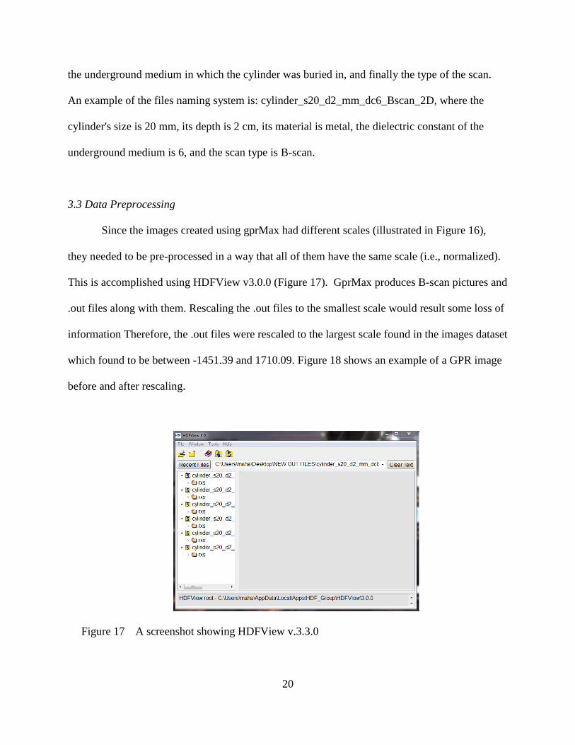
3.3 Data Preprocessing
Since the images created using gprMax had different scales (illustrated in Figure 16),
they needed to be pre-processed in a way that all of them have the same scale (i.e., normalized).
This is accomplished using HDFView v3.0.0 (Figure 17). GprMax produces B-scan pictures and
.out files along with them. Rescaling the .out files to the smallest scale would result some loss of
information Therefore, the .out files were rescaled to the largest scale found in the images dataset
which found to be between -1451.39 and 1710.09. Figure 18 shows an example of a GPR image
before and after rescaling.
Figure 17 A screenshot showing HDFView v.3.3.0

21
Figure 18 Two GPR images showing (L-R) before rescaling; and after rescaling using
HDFView
After rescaling all of the B-scans, they were changed from RGB scale to grey scale, and
then resized from 637x60 to 112x60 in order to reduce the amount of memory needed to train the
proposed convolutional neural nets. Hence, the pre-processing steps in Figure 19 included
rescaling (using HDFView), and changing colour format and resizing (using Matlab), without the
need of any of the complex pre-processing steps (e.g., edge detection, segmentation, support
vector machine (SVM) classifiers, etc).

22
Figure 19 Steps of pre-processing GPR images
3.4 CNN Background
Convolutional neural networks were revolutionized on 2012 when Alex Krizhevsk used
them to win the annual Olympics of computer vision by reducing the classification error record
from 26% to 15% [33]. CNNs are commonly used when data consist of images. They are
categorized as supervised learning, in which data are labeled, unlike unsupervised learning where
data do not need labeling. Convnets are made of layers and information is passed through those
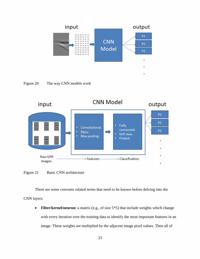
layers. Any CNN model works by taking an image array, where each pixel value in the image is
in a specific range. The output of a CNN model would be a probability of this image being of a
certain class (Figure 20). This is accomplished by training the CNN model using training data.
More specifically, CNNs turns the input images into a set of automatically selected features or
any useful observations (e.g., edges, corners, textures, patterns, etc.). Then, the last block of
layers performs the classification and produces the output using the output layer. The output
layer returns the strength of the network to predict and classify images according to a set of
available classes (Figure 21).
23
Figure 20 The way CNN models work
Figure 21 Basic CNN architecture
There are some convnets related terms that need to be known before delving into the
CNN layers:
• Filter/kernel/neuron: a matrix (e.g., of size 5*5) that include weights which change
with every iteration over the training data to identify the most important features in an
image. These weights are multiplied by the adjacent image pixel values. Then all of

24
these multiplications are summed up to represent a single number. This is done for
every location in the input image producing an activation map or a feature map. It
can be visualized as a flash light that shines over an area of an image and
slides/convolves across all the areas in that image. Its depth should be similar to the
input's depth, 3 in the case of colored images and 1 in the case of gray images. Figure
22 [34] illustrates how the filter works inside the convolutional layer.
• Stride: the number of steps taken by the filter while scanning the images to train the
convolutional net [35].
• Receptive field: the region being shined on using the filter [36].
• Padding: adding new numbers to the borders of the image to preserve its size [35].
An example of zero padding is illustrated in Figure 23 [37].
• Epoch: a single iteration over all the images [31].
• Training data: images used to train the network [31].
• Test data: data used to test that the network works correctly [31].
• Accuracy: the ratio of the number of the truly classified images to the number of
images in the test data [31].
• Mini batch: a small randomly selected subset of training data [31].
• Mini batch accuracy: the percentage of classified images in the subset dataset [31].
• Mini batch loss: the percentage of incorrectly classified images in the subset dataset
[31].

25
Figure 22 The result after convolving a 5*5 filter
Figure 23 Zero padding
The layers usually seen in any convolutional net are the followings (described in the terms
of Matlab R2017b) [37] :
• The features detecting layers:
1. The image input layer: the parameters of this layer include the height, width,
and the channel size of the input images. For gray scale images the channel
size is 1 and for colored images the channel size is 3 corresponding to the RGB
values. Besides manipulating the images size, this layer is capable of
specifying any transformations, such as normalization or data augmentation
(flipping or cropping the data randomly).

26
2. The convolutional layer: this layer takes two arguments. The first argument is
filter size, which includes height and width of the filter that scans along
training dataset. The second argument is number of filters, which determines
the number of feature maps.
3. The ReLu layer: ReLu is an abbreviation for the Rectified Linear Unit
function. Its main purpose is to change any subzero pixel values to zero in
order to accelerates the learning process. The ReLu layer job is mathematically
described in Equation 1 where x is the pixel value.
Max(0,x) (eq. 1)
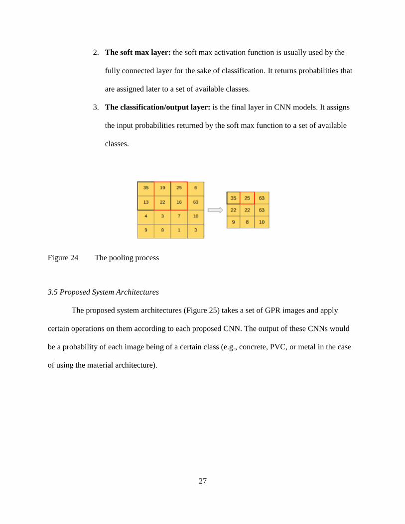
4. The pooling layer: is a down sampling layer that usually follows the
convolutional layer or the activation function. It reduces spatial dimensionality
(i.e., height and width) and computational overhead by discarding insignificant
data and preserving detected features. There are many kinds of pooling layers,
such as average pooling layer and maximum pooling layer that takes the
average/maximum value in a sliding window. The arguments of this layer are:
pool size and stride. The pooling process is illustrated in Figure 24 [37].
• The classification layers:
1. The fully connected layer: one or more of the fully connected layers usually
follows the convolutional layer and the pooling layer. The last fully connected
layer is fully connected with the output of the previous layer. It combines all
the learned features across the previous layers to classify images.
27
2. The soft max layer: the soft max activation function is usually used by the
fully connected layer for the sake of classification. It returns probabilities that
are assigned later to a set of available classes.
3. The classification/output layer: is the final layer in CNN models. It assigns
the input probabilities returned by the soft max function to a set of available
classes.
Figure 24 The pooling process
3.5 Proposed System Architectures
The proposed system architectures (Figure 25) takes a set of GPR images and apply
certain operations on them according to each proposed CNN. The output of these CNNs would
be a probability of each image being of a certain class (e.g., concrete, PVC, or metal in the case
of using the material architecture).

28
Figure 25 Proposed system architectures
3.6 Proposed CNN Models
Applying CNNs on GPR data is a complicated process since there is a massive amount of
convolutional networks' designs with a wide set of configurable parameters (i.e., different filter
sizes, different number of filters, different order of layers, etc.). Therefore, two CNNs were
selected from a set of proposed models by other authors to detect buried objects in GPR images
(i.e., CNN3 [38] and CNN4 [3].). They were slightly modified to match the inputs size and the
desirable outputs of this project. The other two CNNs (i.e., CNN1 and CNN2) were inspired
from Mathworks.com. They have been selected based on their similarity to the recommended
models CNN3 and CNN4.
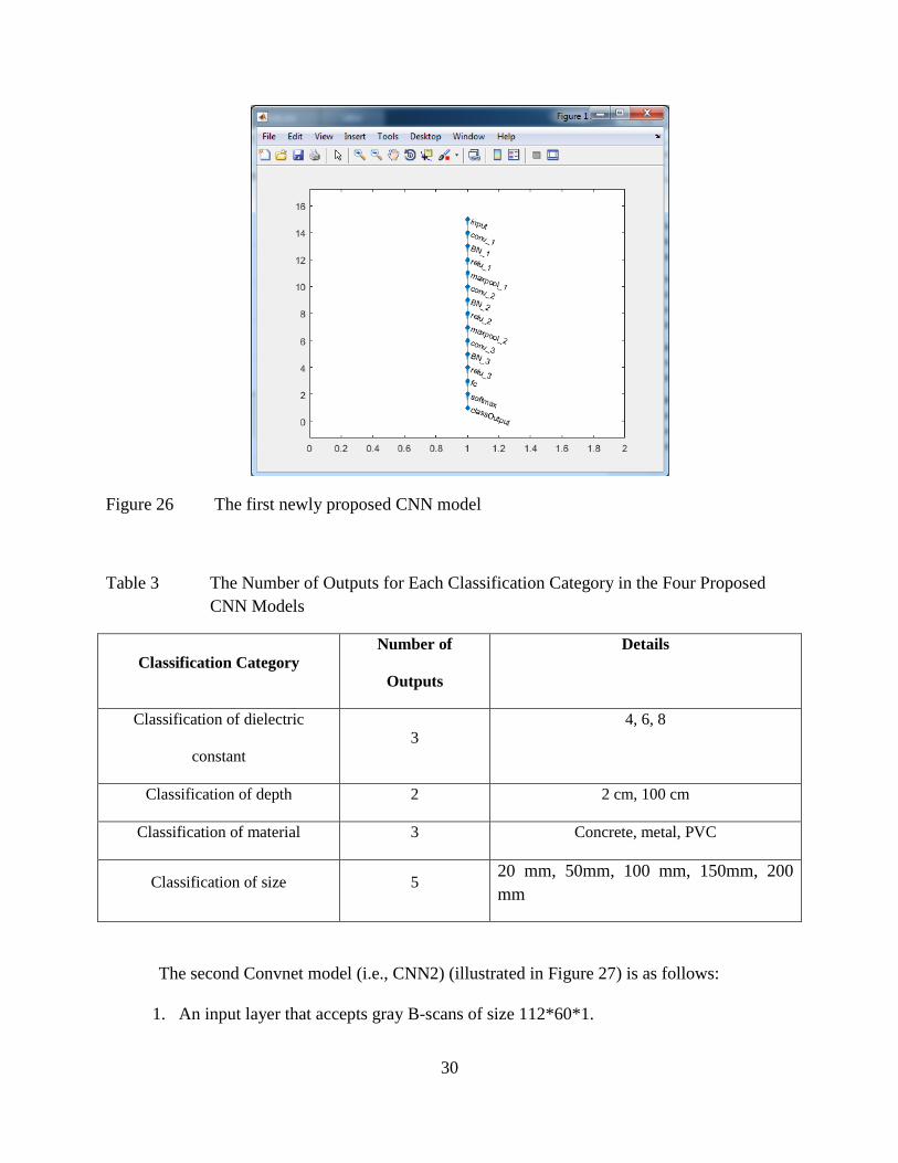
Figure 26 depicts CNN1, the first proposed CNN architecture, which is described as
follows:
1. An input layer that accepts gray B-scans of size 112*60*1.
2. A first convolutional layer with 16 filters of size 3x3, a stride of 1 and padding of size
29
1 (the default settings of stride and padding).
3. A first batch Normalization Layer.
4. A first ReLu layer.
5. A first max pooling layer with pool size 2 and stride of 2.
6. A second convolutional layer with 32 filters of size 3x3, with default stride and
padding.
7. A second batch Normalization Layer.
8. A second ReLu layer.
9. A second max pooling layer with pool size 2 and stride of 2.
10. A third convolutional layer with 64 filters of size 3x3, with default stride and padding.
11. A third batch Normalization Layer.
12. A third ReLu layer.
13. A fully connected layer with different number of outputs (i.e., output size) according
to each classification category (i.e., cylinders size, depth, material, and the dielectric
constant of the underground medium). Table 3 shows the number of outputs for each
classification category using the four proposed CNN models.
14. A soft max layer.
15. A classification layer.
30
Figure 26 The first newly proposed CNN model
Table 3 The Number of Outputs for Each Classification Category in the Four Proposed
CNN Models
Classification Category
Number of
Outputs
Details
Classification of dielectric
constant
3
4, 6, 8
Classification of depth 2 2 cm, 100 cm
Classification of material 3 Concrete, metal, PVC
Classification of size 5 20 mm, 50mm, 100 mm, 150mm, 200
mm
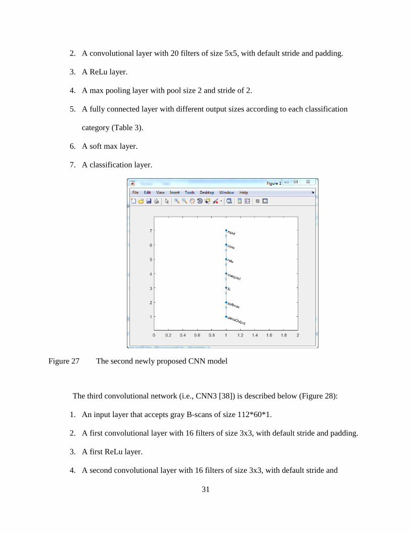
The second Convnet model (i.e., CNN2) (illustrated in Figure 27) is as follows:
1. An input layer that accepts gray B-scans of size 112*60*1.
31
2. A convolutional layer with 20 filters of size 5x5, with default stride and padding.
3. A ReLu layer.
4. A max pooling layer with pool size 2 and stride of 2.
5. A fully connected layer with different output sizes according to each classification
category (Table 3).
6. A soft max layer.
7. A classification layer.
Figure 27 The second newly proposed CNN model
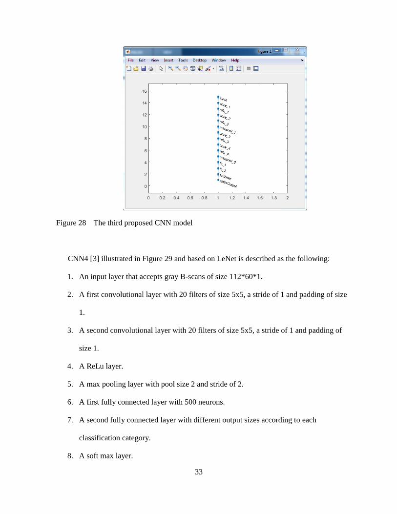
The third convolutional network (i.e., CNN3 [38]) is described below (Figure 28):
1. An input layer that accepts gray B-scans of size 112*60*1.
2. A first convolutional layer with 16 filters of size 3x3, with default stride and padding.
3. A first ReLu layer.
4. A second convolutional layer with 16 filters of size 3x3, with default stride and

32
padding.
5. A second ReLu layer.
6. A first max pooling layer with pool size 2 and stride of 2.
7. A third convolutional layer with 16 filters of size 3x3, with default stride and padding.
8. A third ReLu layer.
9. A fourth convolutional layer with 16 filters of size 3x3, with default stride and
padding.
10. A fourth ReLu layer.
11. A second max pooling layer with pool size 2 and stride of 2.
12. A first fully connected layer with 16 neurons.
13. A fully connected layer with different output sizes according to each classification
category (Table 3).
14. A soft max layer.
15. A classification layer.
33
Figure 28 The third proposed CNN model
CNN4 [3] illustrated in Figure 29 and based on LeNet is described as the following:
1. An input layer that accepts gray B-scans of size 112*60*1.
2. A first convolutional layer with 20 filters of size 5x5, a stride of 1 and padding of size
1.
3. A second convolutional layer with 20 filters of size 5x5, a stride of 1 and padding of
size 1.
4. A ReLu layer.
5. A max pooling layer with pool size 2 and stride of 2.
6. A first fully connected layer with 500 neurons.
7. A second fully connected layer with different output sizes according to each
classification category.
8. A soft max layer.

34
9. A classification layer.
Figure 29 The fourth proposed CNN model
CNN1 and CNN2 where designed in a way that they look similar to CNN3 and CNN4,
while these later two models where chosen because they have shown to be affective with B-scans
[38] [3] (Figure 30). The characteristics of the four architectures used to classify GPR B-scans
are detailed in Table 4. Experimental designs including training options are discussed in Chapter
4.

35
Figure 30 The four Proposed CNN models.
Table 4 The Characteristics of the Proposed CNNs
Proposed/Recommended Number
of
blocks
Number
of
layers
Filter
size
Number of
filters Number of neurons
CNN1 Newly proposed 4 15 3*3 16-32-64 611,529
CNN2 Newly proposed 2 7 5*5 20 309,129
CNN3 Recommended by [38] 5 15 3*3 16-16-32-32 1,296,985
CNN4 Recommended by [3] 3 9 5*5 20 444,029
36
CHAPTER IV
EXPERIMENTS AND RESULTS
All of the four previously mentioned proposed convolutional models were trained using
75% of the synthetic data mentioned in Section 3.2 and tested by the rest of the data (i.e., 25%).
Training the dataset was done on a single CPU using stochastic gradient descent with momentum
(SGDM). SGDM is specified in Equation 2, where ℓ is The iteration number, α is the learning
rate, θ is the parameter vector, E(θ) is the loss function, and ∇E(θ) is the gradient of the loss
function. Each model was used to classify 2D cylinders' scans according to four classification
categories: cylinders' depth, material, size, and dielectric constant of the burying medium.
θℓ+1=θℓ−α∇E(θℓ) (eq. 2)
The steps of the experiment were as follows:
1. Find the effect of adjusting training options on the accuracy of the four CNN
models. The investigated options include:
a. The initial learning rate.
b. Learn Rate Drop Factor and Learn Rate Drop Period. Suggested by [38].
c. The maximum number of epochs.
2. Train the four models using the best combination of the previously mentioned
training options, and then find which architecture works the best.
37
3. Find which of the four classification categories is most accurately classified.
4.1 Using Default Training Options
Layers included within CNN models come with many parameters known as weights. The
initial values of those weights are random. These weights are updated and finalized by training
the network on specific data. Hence, those weights determine how the networks behave when
data is passed through them. Two exactly similar network models will behave differently if they
were trained using different datasets or different training options. Conversely, different models
will behave differently if they were trained using the same training options. Thus, for each
proposed CNN, training options should be investigated to know which subset of them would
produce a better accuracy.
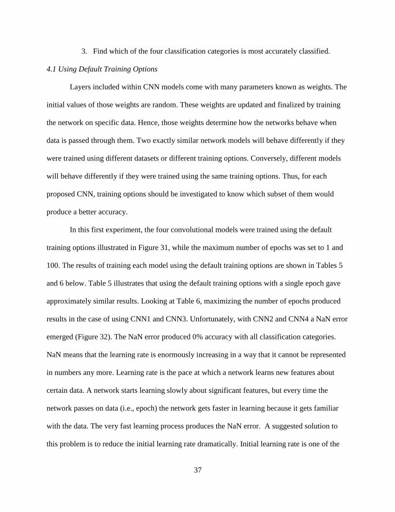
In this first experiment, the four convolutional models were trained using the default
training options illustrated in Figure 31, while the maximum number of epochs was set to 1 and
100. The results of training each model using the default training options are shown in Tables 5
and 6 below. Table 5 illustrates that using the default training options with a single epoch gave
approximately similar results. Looking at Table 6, maximizing the number of epochs produced
results in the case of using CNN1 and CNN3. Unfortunately, with CNN2 and CNN4 a NaN error
emerged (Figure 32). The NaN error produced 0% accuracy with all classification categories.
NaN means that the learning rate is enormously increasing in a way that it cannot be represented
in numbers any more. Learning rate is the pace at which a network learns new features about
certain data. A network starts learning slowly about significant features, but every time the
network passes on data (i.e., epoch) the network gets faster in learning because it gets familiar
with the data. The very fast learning process produces the NaN error. A suggested solution to
this problem is to reduce the initial learning rate dramatically. Initial learning rate is one of the
38
training options. Adjusting the initial learning rate is discussed in detail in the next section.
Figure 31 A screenshot showing the default training options for CNNss
Table 5 Training the Proposed CNNs Using the Default Training Options While the
Maximum Number of Epochs Was Set to 1
Classification
categories
CNN1 CNN2 CNN3 CNN4
Dielectric constant 57.1% 26.1% 33.3% 50%
Depth 50% 50% 50% 36.3%
Material 52.3% 40.4% 33.3% 35.7%
Size 20% 20% 20% 45%
Average 44.8% 34.1% 34.1% 41.7%

39
Table 6 Training the Proposed CNNs Using the Default Training Options While the
Maximum Number of Epochs Was Set to 100
Classification
categories
CNN1 CNN2 CNN3 CNN4
Dielectric constant 97.6% 0% 35.7% 0%
Depth 72.7% 0% 40.9% 0%
Material 97.6% 0% 47.6% 0%
Size 100% 0% 20% 0%
Average 91.9% 0% 36% 0%
Figure 32 A Screenshot showing a 0% classification accuracy because mini batch loss =
NaN
4.2 Adjusting the Initial Learning Rate
The initial learning rate is the pace at which a network starts to learn by about data
features. The default initial learning rate equals 0.0100. This rate was reduced to solve the NaN
problem mentioned in the previous section. The results of adjusting the initial learning rate using
a single epoch for training are shown in Table 7. Comparing Table 7 to Table 5 it was found that
using the adjusted initial learning rate with the four used network models decreased their
accuracy. Nevertheless, the benefit of reducing the initial learning rate emerged when the
number of epochs was increased to 100. Increasing the number of epochs increased the learning

40
rate and produced a NaN error that was solved by decreasing the initial learning rate. Using 100
epochs and comparing Table 8 (after adjusting the rate) to Table 6 (before adjusting the rate), the
adjusted initial learning rate solved the problem of NaN for CNN2 and CNN4, but dropped out
the accuracy rate of CNN1 from an average of 91.9% to 88.5% and CNN3 from 36% to 30.7%.
This means that adjusting the initial learning rate does not always work for the best. It solved the
NaN error for two CNN models (i.e., CNN2 and CNN4), but degraded the performance of both
CNN1 and CNN3.
Table 7 Results After Adjusting the Initial Learning Rate to (0.0001) and Epochs=1
Classification
categories
CNN1 CNN2 CNN3 CNN4
Dielectric constant 33.3% 34.7% 33.3% 11.9%
Depth 50% 52.1% 27.2% 50%
Material 33.3% 23.2% 38.1% 33.3%
Size 40% 30.2% 22.5% 45%
Average 39.1% 35% 30.2% 35%

41
Table 8 Results After Adjusting the Initial Learning Rate to (0.0001) and Epochs=100
Classification
categories
CNN1 CNN2 CNN3 CNN4
Dielectric constant 100% 90.4% 33.3% 57.1%
Depth 59% 40.9% 36.3% 59%
Material 97.6% 80.9% 33.3% 45.2%
Size 97.5% 87.5% 20% 62.5%
Average 88.5% 74.9% 30.7% 55.9%
4.3 Adjusting the Learn Rate Drop Factor and the Learn Rate Drop Period
Learn Rate Drop Factor is the number by which the learning rate is decreased, while
Learn Rate Drop Period is the number of epochs which after it the learning rate will be
decreased. Adjusting these two options was suggested by [38] to increase the models efficiency.
Following [38], the decreasing factor of learning rate was set to 50% every 4 epochs. To see the
effect of these suggested values, a single epoch could not be chosen for training, because the
Learn Rate Drop Period was set to 4 epochs. Therefore, 8 epochs were applied. Furthermore, the
initial learning rate was adjusted for CNN2 and CNN4 to avoid the NaN error. Comparing the
results of applying these parameters before adjusting the Learn Rate Drop Factor and the Learn
Rate Drop Period (Table 9) and after adjusting them (Table 10) it was found that the
performance of CNN1, CNN2 and CNN3 was increased, but the performance of CNN4 was
decreased.

42
Table 9 Epochs=8, and Initial Learning Rate Adjusted to 0.0001 for CNN2 and CNN4
Classification
categories
CNN1 CNN2 CNN3 CNN4
Dielectric constant 64.2% 38.1% 33.3% 33.3%
Depth 54.5% 40.9% 40.9% 59%
Material 47.6% 42.8% 33.3% 45.2%
Size 42.5% 52.5% 20% 35%
Average 52.2% 43.5% 31.8% 43.1%
Table 10 Learn Rate Drop Factor=0.5, Learn Rate Drop Period=4, Epochs=8, and Initial
Learning Rate Adjusted to 0.0001 for CNN2 and CNN4
Classification
categories
CNN1 CNN2 CNN3 CNN4
Dielectric constant 52.3% 50% 33.3% 40.4%
Depth 59% 50% 54.5% 45.4%
Material 61.9% 45.2% 33.3% 23.8%
Size 67.5% 52.5% 20% 25%
Average 60.1% 49.4% 35.2% 33.5%
From the above experiments it was found that training options affect differently on
different kinds of convolutional networks. In other words, the same training options applied on
different networks would produce fluctuated results Thus, Table 11 was created to show which
of the mentioned training options worked good to each of the four networks.

43
Table 11 The Best Combination of the Adjusted Training Options for Each Proposed CNN
Adjusted training option CNN1 CNN2 CNN3 CNN4
Initial learning rate = 0.0001 x x
Learn rate drop factor= 50%, and learn rate drop period= 4 epochs x x x
4.4 Adjusting the Maximum Number of Epochs
Using the combination of adjusted training options in Table 11 along with the right
number of epochs at Table 12 proved promising results. Cylinders based on their sizes, depths,
materials, and the dielectric constant of the underground medium were able to be at least 90%
correctly classified with a fair number of epochs considering the low amount of data. Table 12
illustrates the needed number of epochs to reach at least 90% accuracy using the early suggested
combination of training options (Table 11). The training options were adjusted as follows: initial
learning rate= 0.0001, learn rate drop factor=0.5, and learn rate drop period=4. Noticeably, the
suggested model CNN1 had the best performance with all classification categories with an
average of 60.7 epochs. Furthermore, classifying GPR scans according to the cylinders' materials
was the most accurate, with an average total of 86.7 epochs. The next accurate was classifying
cylinders according to their depth, then size, then dielectric constant of the burying medium
(Table 12).

44
Table 12 The Needed Number of Epochs for Each Model to Achieve an Accuracy of More
Than 90% Using the Training Options Adjustment Combination in Table 11
Classification
categories
CNN1 CNN2 CNN3 CNN4 Average
Dielectric constant 49e 53e 146e 158e 101.5e
Depth 90e 111e 100e 153e 94.5e
Material 56e 60e 136e 200e 86.7e
Size 48e 52e 225e 144e 98.7
Average 60.7e 69e 151.7e 163.7e
In conclusion, it was found from the earlier experiments that there is no single training
option that worked the same for the four suggested convolutional networks. Adjusting the initial
learning rate and the learn rate drop parameters had a two sided effect. They worked perfectly
with some models, but poorly with others, unlike maximizing the number of epoch which always
improved accuracy. A combination of adjusted initial learning rate, learn drop factor, learn drop
period (Table 11), and maximum number of epochs resulted the four CNN models to classify the
GPR dataset more accurately (Table 12). Furthermore, the newly proposed model, CNN1,
showed the best performance using the suggested combination of training options. CNN1 is
differentiated from the other previously mentioned networks by having 3 convolutional layers
with different amount of 3*3 filters. Having a larger number of smaller filters improves the
accuracy of a CNN model because they are able of catching more features [38]. In addition it
was found that classifying the B-scans was more accurate in the case of cylinders' materials.

45
CHAPTER V
SUMMARY AND FUTURE WORK
GPR is a rapidly evolving, non-destructive technology that is used to image the
underground objects. These images are then used to detect and recognize the features of the
buried targets to solve many existing problems such as landmine detection, avalanche victims'
detection, concrete and soil moisture assessment, liquid and soil contamination measurement,
bridge deck inspection, railroad ballast monitoring and many other research projects. Thus, it is a
wide and important research topic. Classifying GPR data with the existence of human factor
needs an enormous amount of experience and time especially when dealing with an excessive
amount of data images. Therefore, an automatic technique is very necessary to solve this issue.
A couple of programmed methods to classify GPR data have been used by researchers
including the accomplishment of using Pattern Recognition, Genetic Programming, Support
Vector Machines, and Neural networks. Detecting images was beyond the scope of this project
since a lot of research experiments were done to deal with this matter. This project focused on
classifying cylinders' B-scans according to their depth, size, material, and the dielectric constant
of the underground medium deploying four different models of convolutional neural networks.
Two of these networks were proposed in this study, while the other two were used by other
authors [38] [3]. These CNNs were trained using different adjusted training options including
initial learning rate, learn rate drop factor, and learn rate drop period which had a positive impact
on a part of the used models. Unlike the maximum number of epochs which worked good with

46
all of the four suggested models. After using the best combination of training options to train the
four models, the first proposed convolutional model, CNN1, showed a superior performance due
to the use of a deep network with a large amount of small filters. Using this model, it was found
that the best results were carried out when GPR B-scans were classified according to the
cylinders' materials and the worst resulted from classifying images according to the dielectric
constant of the burying medium.
Future work on this research includes investigating other training options such as: mini-
batch size, dropout, and validation data. Also, training the first proposed CNN to real GPR data
instead of using simulated images. This data might include images of more complex shapes or
multiple targets. Another suggestion would be replacing 2D images with 3D ones.

47
REFERENCES
[1] A. Venkatachalam, X. Xu, D. Huston, and T. Xia, "Development of a new high speed dual-
channel impulse," IEEE Journal of Selected Topics in Applied Earth Observations and
Remote Sensing, vol. 7, pp. 753-760, Sep. 2013.
[2] A. Andrews, J. Ralston, and M. Tuley, "Research of ground-penetrating radar for detection of
mines and current status and research strategy," Institute for Defense Analyses, Dec.
1999.
[3] S. Lameri, F. Lombardi, P. Bestagini, M. Lualdi, and S. Tubaro, "Landmine detection from
GPR data using convolutional neural networks," European Signal Processing Conference,
Sep. 2017.
[4] S. Ni ,Y. Huang, K. Lo, and D. Lin, "Buried pipe detection by ground penetrating radar using
the discrete wavelet transform," Elsevier, vol. 37, no. 4, pp. 440-448, Jun. 2010.
[5] C. Jaedicke, "Snow mass quantification and avalanche victim search by ground penetrating
radar," Surveys in Geophysics, vol. 24, pp. 431-445, Nov. 2003.
[6] F Fruehauf, A. Heilig, M. Schneebeli, W. Fellin, and O. Scherzer, "Experiments and
algorithms to detect snow avalanche victims using airborne ground-penetrating radar,"
IEEE, vol. 47, pp. 2240 - 2251, Apr. 2009.
[7] Y. Zhang, D. Burns, D. Huston, and T. Xia, "Sand moisture assessment using instantaneous
phase information in ground penetrating radar data," Proceedings of SPIE, Mar. 2015.
[8] J. Daniels, R. Roberts, and M. Vendl, "Ground penetrating radar for the detection of liquid
contaminants," Elsevier, vol. 33, no. 1-3, pp. 195-207, Jan. 1995.
[9] G. Xiujun, W, Shuqiang, W. Xianli, "Detecting three types of contaminated soil with ground
penetrating radar," IEEE, Jun. 2012.
[10] Y. Zhang, P. Candra, G. Wang, and T. Xia, "2-D Entropy and short-time fsourier transform
to leverage GPR data analysis efficiency," IEEE Transactions on Instrumentation and
Measurement, vol. 64, pp. 103-11, Jan. 2015.

48
[11] Y. Zhang, A. Venkatachalam, and T. Xia, "Ground-penetrating radar railroad ballast
inspection with an unsupervised algorithm to boost the region of interest detection
efficiency," Journal of Applied Remote Sensing, vol. 9, Jul. 2015.
[12] Y. Zhang, A.S. Venkatachalam, T. Xia, Y. Xie, and G. Wang, "Data analysis technique to
leverage ground penetrating radar ballast inspection performance," IEEE Radar
Conference, May 2014.
[13] D. Huston, and T. Xia Y. Zhang, "Underground object characterization based on neural
networks for ground penetrating radar data," Proceedings of SPIE, Apr. 2016.
[14] Ground Penetrating Radar (GPR) Underground Locating Services, accessed February 2018,
http://www.global-gpr.com/ground-penetrating-radar.html
[15] C. Wolff, Radar Tutorial, accessed October 2017,
http://www.radartutorial.eu/02.basics/Ground%20penetrating%20radar.en.html
[16] Worltech, accessed January 2018, http://www. worltech.com/eng/product_cscan2.asp
[17] C. Warren, A. Giannopoulos, and I. Giannakis, GprMax: Open Source Software to Simulate
Electromagnetic Wave Propagation for Ground Penetrating Radar, accessed October
2017, http://docs.gprmax.com/en/latest/examples_simple_2D.html
[18] A. Annan, "GPR – trends, history, and future developments," Proceedings of the EAGE
Conference, Jun. 2001.
[19] E. Pasolli, F. Melgani, and M. Donelli, "Automatic analysis of GPR images: a pattern-
recognition approach," IEEE Transactions on Geoscience and Remote Sensing, vol. 47,
Jul. 2009.
[20] J. Kobashigawa, H. Youn, M. Iskander, and Z. Yun, "Classification of buried targets using
ground penetrating radar: comparison between genetic programming and neural
networks," IEEE Antennas and Wireless Propagation Letters, vol. 10, Sep. 2011.
[21] X. Xie, P. Li, and L. Liu, "GPR identification of voids inside concrete based on support
vector machine (SVM) algorithm," 14th International Conference on Ground Penetrating
Radar, Jun. 2013.
[22] M. El-Mahallawy and M. Hashim, "Material classification of underground utilities from
GPR images using DCT-based SVM approach," IEEE, vol. 10, Nov. 2013.
[23] S. Kanafiah, N. Kamal, A. Firdaus, M. Ridzuan, M. Majid, N. Syahirah, I. Ibrahim, Y.
Jusman, A. Zaki, M. Ismail, and C. Abdul Rahman, "Recognition system of underground
object shape using ground penetrating radar datagram," IEEE International Conference
on Control System, Computing and Engineering, Nov. 2015.

49
[24] K. O’Shea and R. Nash, An Introduction to Convolutional Neural Networks, accessed
December 2017,
https://white.stanford.edu/teach/index.php/An_Introduction_to_Convolutional_Neural_N
etworks
[25] M. Bejiga, A. Zeggada, A. Nouffidj, and F. Melgani, "A Convolutional neural network
approach for assisting avalanche search and rescue operations with UAV imagery,"
Remote sensing, vol. 9, Jan. 2017.
[26] R. Higa, Quora, accessed January 2018,
https://www.quora.com/What-are-the-benefits-of-the-backpropagation-algorithm-vs-
estimating-gradient-numerically
[27] R. Sakaguchi, K. Morton, L. Collins, and P. Torrione, "Recognizing subsurface target
responses in ground penetrating radar data using convolutional neural networks,"
Proceedings of SPIE, May 2015.
[28] J. Bralich, D. Reichman, L. Collins, J. Malof, "Improving convolutional neural networks for
buried target detection in ground penetrating radar using transfer learning via
pretraining," Proceedings of SPIE, May 2017.
[29] Kitware, Sandia National Labs, and CSimSoft, Paraview, accessed December 2017.
https://www.paraview.org/
[30] The HDF Group, accessed January 2018, https://support.hdfgroup.org/downloads/
[31] The MathWorks, accessed September 2017,
https://www.mathworks.com/products/new_products/latest_features.html
[32] Turk A., A. Hocaoglu, and A. Vertiy, Subsurface Sensing, 1st ed. Wiley, 2011.
[33] A. Krizhevsky, I. Sutskever, and G. Hinton, "ImageNet classification with deep
convolutional neural networks," NIPS, 2012.
[34] M. Nielsen, Deep Learning, accessed September 2017,
http://neuralnetworksanddeeplearning.com/chap6.html
[35] A. Deshpande, A Beginner's Guide to Understanding Convolutional Neural Networks Part 2,
accessed December 2017,
https://adeshpande3.github.io/A-Beginner%27s-Guide-To-Understanding-Convolutional-
Neural-Networks-Part-2/
[36] A. Deshpande, A Beginner's Guide to Understanding Convolutional Neural Networks,
accessed December 2017,

50
https://adeshpande3.github.io/adeshpande3.github.io/A-Beginner%27s-Guide-To-
Understanding-Convolutional-Neural-Networks/
[37] A. Saxena, Convolutional Neural Networks (CNNs): An Illustrated Explanation, accessed
January 2018,
https://xrds.acm.org/blog/2016/06/convolutional-neural-networks-cnns-illustrated-
explanation/
[38] D. Reichman, L. Collins, and J. Malof, "Some good practices for applying convolutional
neural networks to buried threat detection in ground penetrating radar," IEEE, Jun. 2017.

51
VITA
Maha Almaimani was born in Madinah, Saudi Arabia, to Habib Almaimani and Jawaher
Almowalled on November 30, 1989. She is the oldest sister of six siblings. She attended the sixth
high school for females in Madinah and got her Bachelor's in Computer Science from Taibah
University in 2012. Almaimani received a full scholarship from the Saudi Arabian Cultural
Mission to advance her education. She graduated with a Master's of Science from the University
of Tennessee at Chattanooga in Computer Science in May 2018.