Discussion Papers in Economics

________________________________________ Discussion Paper No. 14/02

Classifying Exchange Rate Regimes by Regression Methods

Michael Bleaney and Mo Tian

April 2014

____________________________________________________

2014 DP 14/02

-0-

Classifying Exchange Rate Regimes by

Regression Methods

Michael Bleaney and Mo Tian

School of Economics, University of Nottingham

Abstract

A new and easily implemented regression method is proposed for distinguishing floating

from pegged regimes, whilst simultaneously identifying anchors of pegged currencies. The

method can distinguish pegs with occasional devaluations from floats, and can be used to

generate annual regime classifications. The method largely confirms the accuracy of the

IMF’s de facto classification, but also shows that a significant minority of managed floats is

close to being US dollar pegs. Even flexible managed floats have a strong tendency to track

the US dollar.

Keywords: exchange rates, currency pegs, trade

JEL No.: F31

Corresponding author: Professor M F Bleaney, School of Economics, University of Nottingham, Nottingham NG7 2RD. e-

mail: michael.bleaney@nottingham.ac.uk. Tel. +44 115 951 5464. Fax +44 116 951 4159.

-1-

1 Introduction

Until 1998 the International Monetary Fund reported only a country’s self-declared exchange

rate regime, chosen from amongst a defined set of categories such as various types of peg,

managed floating or independently floating (see Habermeier et al., 2009, Appendix B, for a

brief history of the IMF classification system). Dissatisfaction with the resulting outcomes,

eloquently expressed by Calvo and Reinhart (2002), led to the development of alternative

methods based on factual data such as exchange rate movements, reserve volatility and

interest rate differentials (Levy-Yeyati and Sturzenegger, 2005; Reinhart and Rogoff, 2004;

Shambaugh, 2004). The IMF also began to record its own de facto assessment of the regime,

alongside the reported de jure classification, using the same taxonomy. The weakness of this

effort is that it conspicuously failed to develop a new consensus in classifying exchange rate

regimes, since the new systems showed a low correlation with one another (Bleaney and

Francisco, 2007; Frankel and Wei, 2008).

The schemes that seek to produce an alternative to the IMF classification by calendar

year use different statistical criteria. Levy-Yeyati and Sturzenegger (2005) use cluster

analysis based on movements in exchange rates, international reserves and interest rates.

Reinhart and Rogoff (2004) prefer to use parallel-market exchange rates (if they exist), and

discount large movements in up to 20% of observations, in an attempt to distinguish one-time

devaluations from floats. Shambaugh (2004) defines a peg by small monthly exchange rate

movements in up to eleven out of twelve months.

None of these approaches uses regression methods. Regression methods have been

successfully used to identify the basket of anchor currencies to which a currency is pegged

(Frankel and Wei, 1995). More recently, Bénassy-Quéré et al. (2006) and Frankel and Wei

(2008) have independently suggested that similar regression methods can distinguish pegs

from floats as well. In this paper, we pursue a similar line of inquiry that, in our view,

-2-

improves on previous work. We show that regression analysis can be used to generate

statistics that distinguish floats from pegs, including those with occasional devaluations, with

a high degree of accuracy. It is also a simple way of generating annual regime classifications,

requiring only end-of-month exchange rate data.

The rest of the paper is organised as follows. In Section Two, previous approaches to

exchange rate regime classification by regression methods are reviewed. Our alternative is

presented in Section Three. Section Four shows the results of our method by IMF de facto

regime category, applied to two separate periods: 1999-2005 and 2006-13. Some illustrative

examples are given in Section Five. In Section Six robustness to the choice of numéraire

currency is discussed. Section Seven examines managed floats more deeply. Section Eight

investigates whether the system can be used to generate annual regime classifications.

Conclusions are presented in Section Nine.

2 Literature Review

The standard regression specification for identifying the basket of currencies to which

currency i is pegged (e.g. Frankel and Wei, 1995) relates exchange rate movements of

currency i against some numéraire currency N to movements of potential anchor currencies

against N:

( ) ( ) ( ) ( ) (1)

where USD is the US dollar, EUR is the euro, YEN is the Japanese yen, E(i, N) is the number

of units of currency i per unit of currency N, and is the first-difference operator. If

currency i is pegged to a single one of these currencies, the coefficient of that currency

-3-

should be one, and of the others zero; if the basket is correctly identified, the three

coefficients should sum to one.

The issue is whether a similar equation can also distinguish floats from pegs.

Bénassy-Quéré et al. (2006) avoid the choice of a numéraire currency by noting that, if

b+c+d = 1, then a weighted average of exchange rates of currency i against the three anchors

should remain unchanged:

( ) ( ) ( ) if b+c+d = 1 (2)

After estimating equation (2), the authors focus on the estimates of the individual coefficients

b, c and d. They identify a currency as floating only if none of them is significantly different

from zero. This approach appears to suffer from two drawbacks. One is that, because of the

focus on statistical significance, the standard errors of the coefficients could have as much

influence on the result as the point estimates. The other is that, given the constraint that the

estimated coefficients must sum to one, the test is biased towards rejecting the null; and

indeed less than 10% of the sample is identified as floats (Bénassy-Quéré et al., 2006, Table

3). As we shall see later, even freely floating currencies tend to co-move with others with

which they have strong trading links, and are therefore likely in many cases to have non-zero

euro or US dollar coefficients.

Frankel and Wei (2008) augment equation (1) with an exchange market pressure

variable (EMP), which is equal to the log changes in the exchange rate of currency i against N

minus changes in the logarithm of the ratio of international reserves to the monetary base.

They thus estimate:

( ) ( ) ( ) ( )

-4-

(3)

In fact Frankel and Wei arrive at this specification by including the British pound as an

additional anchor, and then subtracting the pound-numéraire exchange rate from all the other

exchange rate variables to impose the condition that the basket weights sum to one, without

noticing that this procedure is equivalent to estimating a regression with unrestricted basket

weights using the pound as numéraire.1 They focus on the coefficient of this EMP variable,

arguing that it will be close to zero for pegs, and significantly different from zero for floats.

They broadly confirm this pattern using twenty example currencies. Slavov (2013) applies

this method to investigate the behaviour of nominally floating currencies in sub-Saharan

Africa.

Apart from the fact that the test is not infallible (Australia is an example, as Frankel

and Wei point out), there are some econometric problems here. One component of the EMP

variable is the dependent variable itself, so that component should always have a coefficient

of one, as well as being necessarily correlated with the error term, which introduces bias into

the estimates. The reserves component is also endogenous to exchange rate changes because

the money supply is denominated in domestic currency and reserves in foreign currency.

When the exchange rate depreciates, the ratio of reserves to the monetary base will tend to

increase even if reserves remain unchanged.

3 A New Approach

In this paper we start from the position that, for identifying the type of regime (as opposed to

the possible basket of anchor currencies), the appropriate statistics from a regression equation

1 This arises because, for any currency j, ln E(j, N) – ln E(GBP, N) = ln E(j, GBP). The original numéraire

simply disappears from the estimated equation, which reduces to an unrestricted regression with the GBP as

numéraire.

-5-

like (1) should be based on the volatility and pattern of residuals rather than the estimated

coefficients. At a second stage, if the relevant statistics indicate a peg by whatever criterion is

chosen, then the coefficients can be used to identify the anchor basket.

Our baseline regression is:

( ) ( ) ( ) (4)

The numéraire currency is the Swiss franc. Initially we included the Japanese yen as well,

as in equation (1), but its coefficients were almost always insignificant. Instead we use the

yen as an alternative numéraire, to check the sensitivity of the results to the choice of

numéraire. For some currencies we added other potential anchor currencies to the equation,

as follows:

South African Rand – added for Botswana, Lesotho, Namibia and Swaziland.

Indian Rupee – added for Bangladesh, Bhutan, Maldives, Nepal, Pakistan, Seychelles and Sri

Lanka.

Australian and New Zealand Dollars – added for Fiji, Kiribati, Samoa, Solomon Islands,

Tonga and Vanuatu.

Singapore Dollar – added for Brunei.

We have also experimented with adding the change in the ratio of international

reserves to the monetary base (lagged, over months t-4 to t-1, to deal with the endogeneity

issue). Since this variable was rarely significant, we decided to omit it; doing so helps to

reduce the data requirements for implementing our procedure.

To measure volatility, we use the root mean square error (RMSE) and the R-squared

of equation (4). We expect the RMSE to be low and the R-squared to be high for pegs, and

-6-

vice versa for floats. In the remainder of the paper we discuss the performance of these

statistics in distinguishing floats from pegs.

4 Main Results by IMF de facto Regime

In this section we show the results of estimating equation (4) for two separate periods:

January 1999 to December 2005 (83 months), and January 2006 to June 2013 (90 months).

We omitted any countries which had switched de facto regime, according to the IMF, during

the period. These periods give us two samples of more than 80 monthly observations each.

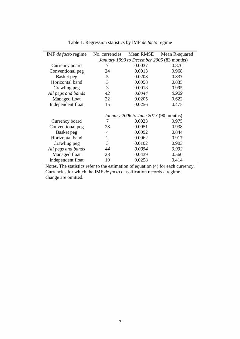
Table 1 shows the means by IMF de facto regime. The top panel of Table 1 refers to the

earlier period and the bottom panel to the later period.

What emerges quite clearly is that floats look different from pegs. Pegs tend to have

RMSEs below or close to 0.01, whereas for independent floats the RMSE tends to be above

0.02, and the average in each period is above 0.025. This pattern is mirrored in the R-

squareds. For independent floats the R-squared averages below 0.5 in each period. For pegs

of any kind, the average R-squared is always greater than 0.8, and in most cases considerably

closer to one than that. For pegs and bands as a whole, the average RMSE is 0.0044 in 1999-

2005 and 0.0055 in 2006-13, and the average R-squared is 0.93 in each period. Managed

floats have an average RMSE of 0.0205 in 1999-2005 and 0.0245 in 2006-13, with average

R-squareds of 0.622 and 0.630 respectively.

-7-

Table 1. Regression statistics by IMF de facto regime

IMF de facto regime No. currencies Mean RMSE Mean R-squared

January 1999 to December 2005 (83 months)

Currency board 7 0.0037 0.870

Conventional peg 24 0.0013 0.968

Basket peg 5 0.0208 0.837

Horizontal band 3 0.0058 0.835

Crawling peg 3 0.0018 0.995

All pegs and bands 42 0.0044 0.929

Managed float 22 0.0205 0.622

Independent float 15 0.0256 0.475

January 2006 to June 2013 (90 months)

Currency board 7 0.0023 0.975

Conventional peg 28 0.0051 0.938

Basket peg 4 0.0092 0.844

Horizontal band 2 0.0062 0.917

Crawling peg 3 0.0102 0.903

All pegs and bands 44 0.0054 0.932

Managed float 28 0.0439 0.560

Independent float 10 0.0258 0.414

Notes. The statistics refer to the estimation of equation (4) for each currency.

Currencies for which the IMF de facto classification records a regime

change are omitted.

-8-

This difference in means is encouraging but not necessarily compelling. It does not tell us

how much overlap there is between the distributions. For example the high average RMSE of

0.0208 for the five basket pegs in the 1999-2005 period suggests that one or two of them may

look quite similar to floats according to these statistics. Indeed that is the case: the Libyan

dinar has an RMSE of 0.081 and an R-squared of 0.021 in that period. A particular issue is

the devaluation of a pegged currency. This is not a regime change, but in the regression it

would produce a large residual for that month. This would raise the RMSE and reduce the R-

squared, and could distort the other coefficients, as we show by an example in the next

section.

A symptom of one or more devaluations should be a distinctive pattern of residuals.

In the event of a devaluation, positive residuals (representing a depreciation relative to the

Swiss franc that is not explained by movements in the US dollar or the euro against the Swiss

franc) should be relatively infrequent but occasionally large, and negative residuals should be

on average much smaller but much more numerous. In other words, the residuals in this case

should be markedly positively skewed. For genuine floats, we do not expect the residuals to

be skewed in this way. In fact in the sample shown in Table 1, skewness never exceeds two

in absolute value for independent floats, but quite frequently does so for other regimes.

This suggests that the skewness of residuals can be used to identify months with

possible parity changes. For each of these months, a dummy variable that is equal to one for

that month only, and zero otherwise, can be added to the regression. The regression can then

be rerun, and the RMSE and R-squared re-examined. For pegs with occasional devaluations,

the resulting statistics should now be in the expected range for pegs; for floats that just

happened to have an usually large movement in one month, these statistics should be much

less markedly affected by the inclusion of the dummies.

-9-

Table 2. Regression statistics by IMF de facto regime

with a dummy for a single outlying month

IMF de facto regime No. currencies Mean RMSE Mean R-squared

January 1999 to December 2005 (83 months)

Currency board 7 (2) 0.0034 0.884

Conventional peg 24 (6) 0.0008 0.973

Basket peg 5 (2) 0.0090 0.932

Horizontal band 3 (1) 0.0057 0.845

Crawling peg 3 (0) 0.0018 0.995

All pegs and bands 42 (11) 0.0026 0.946

Managed float 22 (5) 0.0185 0.680

Independent float 15 (0) 0.0256 0.475

January 2006 to June 2013 (90 months)

Currency board 7 (2) 0.0022 0.975

Conventional peg 28 (6) 0.0030 0.970

Basket peg 4 (1) 0.0044 0.967

Horizontal band 2 (0) 0.0062 0.917

Crawling peg 3 (1) 0.0086 0.910

All pegs and bands 44 (10) 0.0035 0.964

Managed float 28 (9) 0.0222 0.662

Independent float 10 (2) 0.0252 0.439

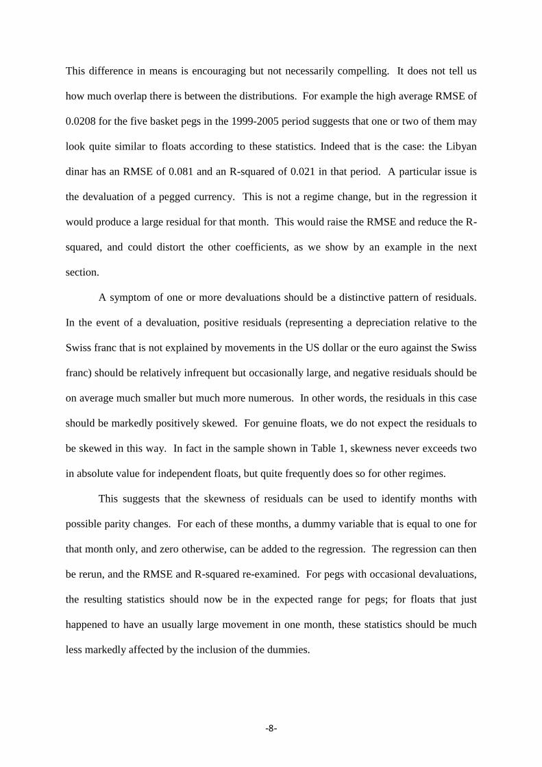
Notes. The statistics refer to the estimation of equation (4) for each currency,

with the addition of the most significant dummy variable for a single

outlying month if the F-statistic for that dummy variable’s exclusion from

the regression exceeds 30. Figures in parentheses are the number of

currencies for which a dummy was included, using this criterion. Currencies

for which the IMF de facto classification records a regime change are

omitted.

-10-

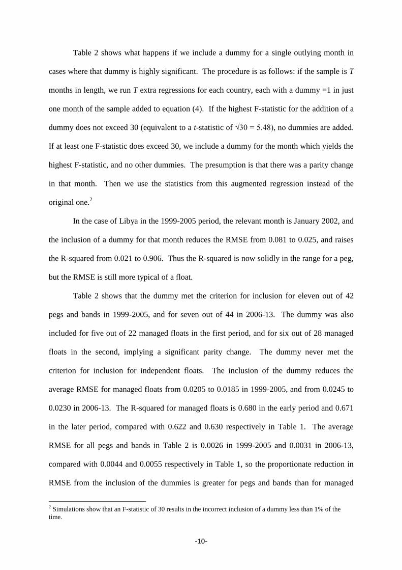
Table 2 shows what happens if we include a dummy for a single outlying month in

cases where that dummy is highly significant. The procedure is as follows: if the sample is T

months in length, we run T extra regressions for each country, each with a dummy =1 in just

one month of the sample added to equation (4). If the highest F-statistic for the addition of a

dummy does not exceed 30 (equivalent to a t-statistic of √30 = 5.48), no dummies are added.

If at least one F-statistic does exceed 30, we include a dummy for the month which yields the

highest F-statistic, and no other dummies. The presumption is that there was a parity change

in that month. Then we use the statistics from this augmented regression instead of the

original one.2

In the case of Libya in the 1999-2005 period, the relevant month is January 2002, and

the inclusion of a dummy for that month reduces the RMSE from 0.081 to 0.025, and raises

the R-squared from 0.021 to 0.906. Thus the R-squared is now solidly in the range for a peg,

but the RMSE is still more typical of a float.

Table 2 shows that the dummy met the criterion for inclusion for eleven out of 42

pegs and bands in 1999-2005, and for seven out of 44 in 2006-13. The dummy was also

included for five out of 22 managed floats in the first period, and for six out of 28 managed

floats in the second, implying a significant parity change. The dummy never met the

criterion for inclusion for independent floats. The inclusion of the dummy reduces the

average RMSE for managed floats from 0.0205 to 0.0185 in 1999-2005, and from 0.0245 to

0.0230 in 2006-13. The R-squared for managed floats is 0.680 in the early period and 0.671

in the later period, compared with 0.622 and 0.630 respectively in Table 1. The average

RMSE for all pegs and bands in Table 2 is 0.0026 in 1999-2005 and 0.0031 in 2006-13,

compared with 0.0044 and 0.0055 respectively in Table 1, so the proportionate reduction in

RMSE from the inclusion of the dummies is greater for pegs and bands than for managed

2 Simulations show that an F-statistic of 30 results in the incorrect inclusion of a dummy less than 1% of the

time.

-11-

floats. The 1999-2005 average R-squared for all pegs and bands rises from 0.929 in Table 1

to 0.941 in Table 2, and the 2006-13 average R-squared for all pegs and bands rises from

0.942 to 0.971.

Overall, these results suggest that a search for outlying residuals in equation (4)

should enable pegs with occasional devaluations to be distinguished from genuine floats.

Managed floats are difficult to evaluate in general, because their behaviour depends

very much on how they are managed. As we shall show later, our methodology reveals that,

while some seem relatively lightly managed, others are quite close to a form of peg, usually

to the US dollar.

5 Some Examples

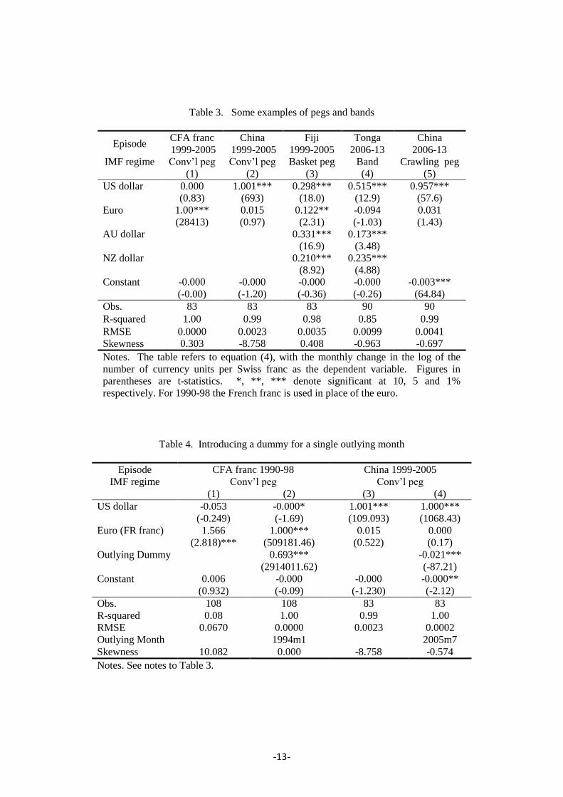
Table 3 gives some examples for pegs and bands (target zones wider than ±1%). In the first

column, the CFA franc from 1999 to 2005 is typical of an exact peg to a single currency: the

US dollar coefficient is zero, the euro coefficient is exactly 1.00, the R-squared is 1.00 and

the RMSE is 0.000. Typical of a slightly looser peg is China from 1999 to 2005, shown in

column (2): the US dollar coefficient is 1.001, with a t-statistic of 693, the euro coefficient is

0.015 and insignificant, the R-squared is 0.99 and the RMSE is 0.0023.

An example of a basket peg (Fiji 1999-2005) is given in column (3): all four

currencies have weights significantly different from zero, the R-squared is 0.98 and the

RMSE is 0.0035. In column (4), Tonga 2006-13 shows the difference between a peg and a

band. The US dollar, the Australian dollar and the New Zealand dollar all have significant

coefficients, but the R-squared is lower than for Fiji, at 0.85, and the RMSE is higher

(0.0099). In column (5), China 2006-13 is a good example of a crawling peg (in this case an

appreciating one). The constant is significant and implies an appreciation of about 0.3% per

-12-

month, but the other statistics are typical of a peg, with an R-squared of 0.99 and an RMSE of

0.0041.

In all of these cases except China 1999-2005, the skewness of the residuals is small in

absolute terms, which suggests that there was no parity change during the period. In the case

of China 1999-2005, skewness is -8.76, which indicates an appreciation at some date. Table

4 shows the effects of introducing a dummy for an outlying month for two cases: the CFA

franc, which was devalued by a very large amount in January 1994, from January 1990 to

December 1998, and China 1999-2005. It can be seen that, for the CFA franc, the January

1994 episode greatly affects the results: without the dummy variable for that month (column

1), the R-squared is only 0.08, and the RMSE is extremely high, at 0.0670. Even the French

franc coefficient is distorted, at 1.566 rather than 1.00. Only the residual skewness of 10.08

indicates that this is the effect of one or more large devaluations rather than floating. Once

the January 1994 dummy is included (column 2), the fit is perfect and the French franc

coefficient is exactly one.

In the case of China 1999-2005, introducing a dummy for July 2005 (column 4 of

Table 4) reduces skewness from -8.76 to -0.58, even though the estimated appreciation in that

month is very small (2.1%).

-13-

Table 3. Some examples of pegs and bands

Episode CFA franc

1999-2005

China

1999-2005

Fiji

1999-2005

Tonga

2006-13

China

2006-13

IMF regime Conv’l peg Conv’l peg Basket peg Band Crawling peg

(1) (2) (3) (4) (5)

US dollar 0.000 1.001*** 0.298*** 0.515*** 0.957***

(0.83) (693) (18.0) (12.9) (57.6)

Euro 1.00*** 0.015 0.122** -0.094 0.031

(28413) (0.97) (2.31) (-1.03) (1.43)

AU dollar 0.331*** 0.173***

(16.9) (3.48)

NZ dollar 0.210*** 0.235***

(8.92) (4.88)

Constant -0.000 -0.000 -0.000 -0.000 -0.003***

(-0.00) (-1.20) (-0.36) (-0.26) (64.84)

Obs. 83 83 83 90 90

R-squared 1.00 0.99 0.98 0.85 0.99

RMSE 0.0000 0.0023 0.0035 0.0099 0.0041

Skewness 0.303 -8.758 0.408 -0.963 -0.697

Notes. The table refers to equation (4), with the monthly change in the log of the

number of currency units per Swiss franc as the dependent variable. Figures in

parentheses are t-statistics. *, **, *** denote significant at 10, 5 and 1%

respectively. For 1990-98 the French franc is used in place of the euro.

Table 4. Introducing a dummy for a single outlying month

Episode CFA franc 1990-98 China 1999-2005

IMF regime Conv’l peg Conv’l peg

(1) (2) (3) (4)

US dollar -0.053 -0.000* 1.001*** 1.000***

(-0.249) (-1.69) (109.093) (1068.43)

Euro (FR franc) 1.566 1.000*** 0.015 0.000

(2.818)*** (509181.46) (0.522) (0.17)

Outlying Dummy 0.693*** -0.021***

(2914011.62) (-87.21)

Constant 0.006 -0.000 -0.000 -0.000**

(0.932) (-0.09) (-1.230) (-2.12)

Obs. 108 108 83 83

R-squared 0.08 1.00 0.99 1.00

RMSE 0.0670 0.0000 0.0023 0.0002

Outlying Month 1994m1 2005m7

Skewness 10.082 0.000 -8.758 -0.574

Notes. See notes to Table 3.

-14-

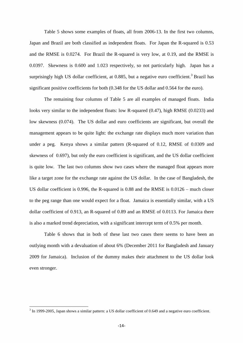
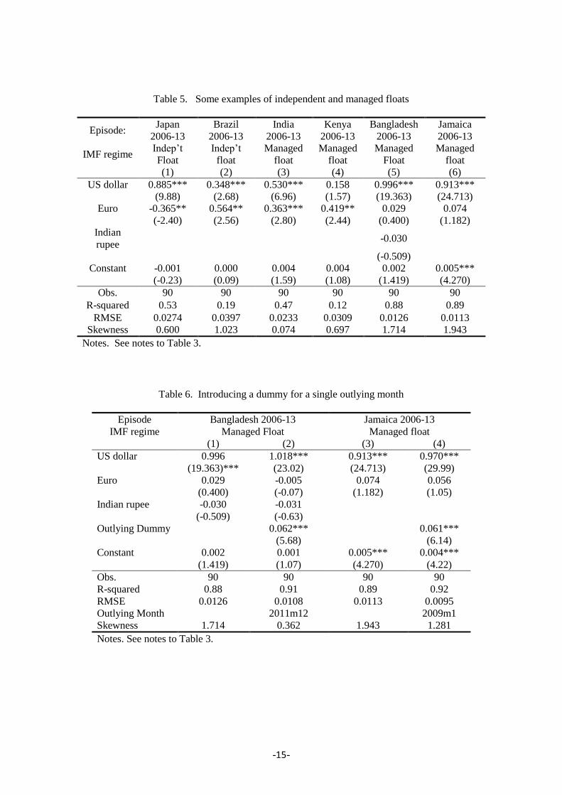
Table 5 shows some examples of floats, all from 2006-13. In the first two columns,

Japan and Brazil are both classified as independent floats. For Japan the R-squared is 0.53

and the RMSE is 0.0274. For Brazil the R-squared is very low, at 0.19, and the RMSE is

0.0397. Skewness is 0.600 and 1.023 respectively, so not particularly high. Japan has a

surprisingly high US dollar coefficient, at 0.885, but a negative euro coefficient.3 Brazil has

significant positive coefficients for both (0.348 for the US dollar and 0.564 for the euro).

The remaining four columns of Table 5 are all examples of managed floats. India

looks very similar to the independent floats: low R-squared (0.47), high RMSE (0.0233) and

low skewness (0.074). The US dollar and euro coefficients are significant, but overall the

management appears to be quite light: the exchange rate displays much more variation than

under a peg. Kenya shows a similar pattern (R-squared of 0.12, RMSE of 0.0309 and

skewness of 0.697), but only the euro coefficient is significant, and the US dollar coefficient

is quite low. The last two columns show two cases where the managed float appears more

like a target zone for the exchange rate against the US dollar. In the case of Bangladesh, the

US dollar coefficient is 0.996, the R-squared is 0.88 and the RMSE is 0.0126 – much closer

to the peg range than one would expect for a float. Jamaica is essentially similar, with a US

dollar coefficient of 0.913, an R-squared of 0.89 and an RMSE of 0.0113. For Jamaica there

is also a marked trend depreciation, with a significant intercept term of 0.5% per month.

Table 6 shows that in both of these last two cases there seems to have been an

outlying month with a devaluation of about 6% (December 2011 for Bangladesh and January

2009 for Jamaica). Inclusion of the dummy makes their attachment to the US dollar look

even stronger.

3 In 1999-2005, Japan shows a similar pattern: a US dollar coefficient of 0.649 and a negative euro coefficient.

-15-

Table 5. Some examples of independent and managed floats

Episode: Japan

2006-13

Brazil

2006-13

India

2006-13

Kenya

2006-13

Bangladesh

2006-13

Jamaica

2006-13

IMF regime Indep’t

Float

Indep’t

float

Managed

float

Managed

float

Managed

Float

Managed

float

(1) (2) (3) (4) (5) (6)

US dollar 0.885*** 0.348*** 0.530*** 0.158 0.996*** 0.913***

(9.88) (2.68) (6.96) (1.57) (19.363) (24.713)

Euro -0.365** 0.564** 0.363*** 0.419** 0.029 0.074

(-2.40) (2.56) (2.80) (2.44) (0.400) (1.182)

Indian

rupee -0.030

(-0.509)

Constant -0.001 0.000 0.004 0.004 0.002 0.005***

(-0.23) (0.09) (1.59) (1.08) (1.419) (4.270)

Obs. 90 90 90 90 90 90

R-squared 0.53 0.19 0.47 0.12 0.88 0.89

RMSE 0.0274 0.0397 0.0233 0.0309 0.0126 0.0113

Skewness 0.600 1.023 0.074 0.697 1.714 1.943

Notes. See notes to Table 3.

Table 6. Introducing a dummy for a single outlying month

Episode Bangladesh 2006-13 Jamaica 2006-13

IMF regime Managed Float Managed float

(1) (2) (3) (4)

US dollar 0.996 1.018*** 0.913*** 0.970***

(19.363)*** (23.02) (24.713) (29.99)

Euro 0.029 -0.005 0.074 0.056

(0.400) (-0.07) (1.182) (1.05)

Indian rupee -0.030 -0.031

(-0.509) (-0.63)

Outlying Dummy 0.062*** 0.061***

(5.68) (6.14)

Constant 0.002 0.001 0.005*** 0.004***

(1.419) (1.07) (4.270) (4.22)

Obs. 90 90 90 90

R-squared 0.88 0.91 0.89 0.92

RMSE 0.0126 0.0108 0.0113 0.0095

Outlying Month 2011m12 2009m1

Skewness 1.714 0.362 1.943 1.281

Notes. See notes to Table 3.

-16-

6 The Choice of Numéraire

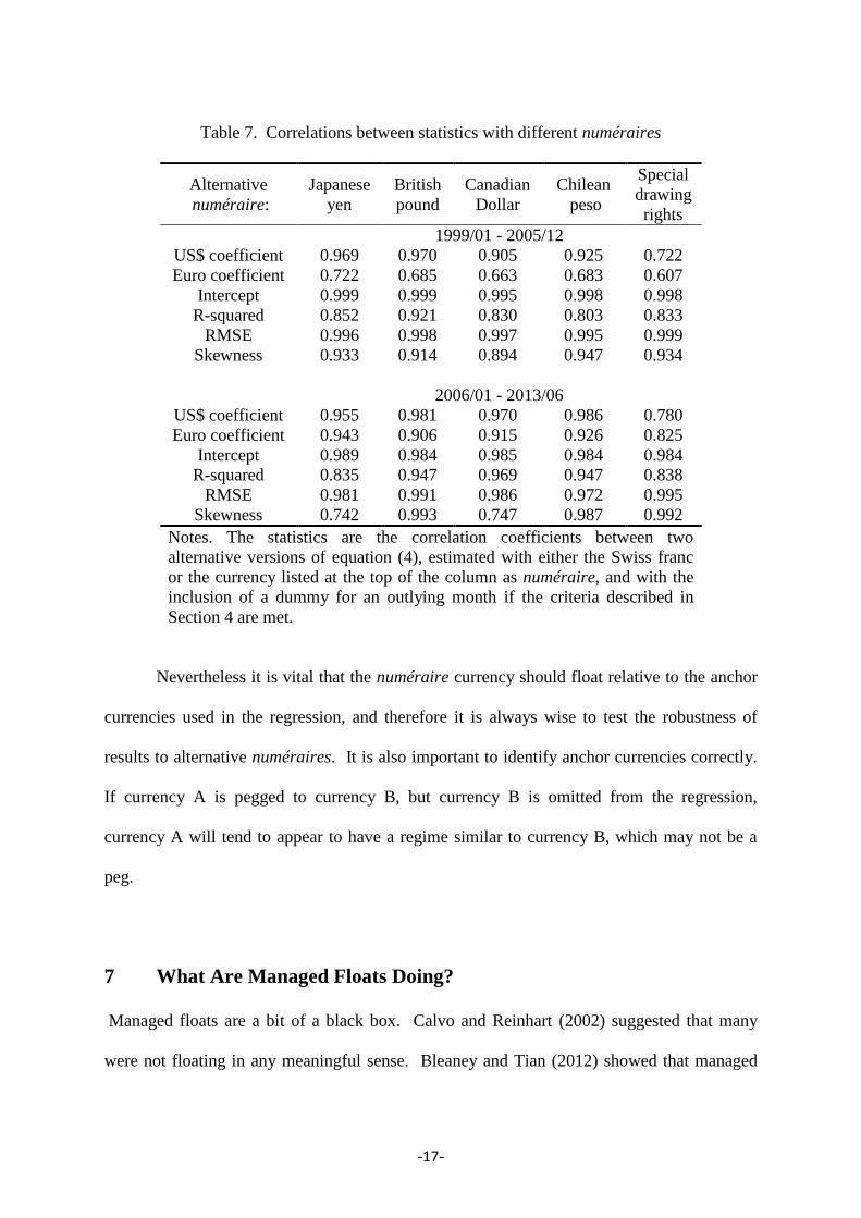
How much difference does the choice of numéraire make? Table 7 shows the correlation of

various regression statistics using other independently floating currencies as alternative

numéraires to the Swiss franc. The correlations are generally high. The R-squared, RMSE

and skewness always have correlations above 0.8, and in more than half the cases above 0.9.

The correlations for the intercept coefficient are particularly high, always exceeding 0.95.

The correlations for the US dollar coefficient always exceed 0.9, except in the case of the

SDR, for which the correlation is 0.722 in 1999-2005 and 0.760 in 2006-13. These lower

correlations no doubt reflect the weight of the US dollar in the SDR basket. For the euro

coefficients, the correlations are also lower for the SDR than for the other currencies,

although to a lesser degree, probably because the weight of the euro in the SDR basket is less

than that of the US dollar. For the euro coefficient, there is a marked difference between the

two periods. In 2006-13 the euro coefficient correlations for currencies other than the SDR

always exceed 0.9, whereas in 1999-2005 they lie in the range 0.66 to 0.73. This may reflect

the fact that the Swiss franc was particularly stable against the euro in this period, making the

euro coefficient harder to estimate when the Swiss franc is used as the numéraire.

-17-

Table 7. Correlations between statistics with different numéraires

Alternative

numéraire:

Japanese

yen

British

pound

Canadian

Dollar

Chilean

peso

Special

drawing

rights

1999/01 - 2005/12

US$ coefficient 0.969 0.970 0.905 0.925 0.722

Euro coefficient 0.722 0.685 0.663 0.683 0.607

Intercept 0.999 0.999 0.995 0.998 0.998

R-squared 0.852 0.921 0.830 0.803 0.833

RMSE 0.996 0.998 0.997 0.995 0.999

Skewness 0.933 0.914 0.894 0.947 0.934

2006/01 - 2013/06

US$ coefficient 0.955 0.981 0.970 0.986 0.780

Euro coefficient 0.943 0.906 0.915 0.926 0.825

Intercept 0.989 0.984 0.985 0.984 0.984

R-squared 0.835 0.947 0.969 0.947 0.838

RMSE 0.981 0.991 0.986 0.972 0.995

Skewness 0.742 0.993 0.747 0.987 0.992

Notes. The statistics are the correlation coefficients between two

alternative versions of equation (4), estimated with either the Swiss franc

or the currency listed at the top of the column as numéraire, and with the

inclusion of a dummy for an outlying month if the criteria described in

Section 4 are met.

Nevertheless it is vital that the numéraire currency should float relative to the anchor

currencies used in the regression, and therefore it is always wise to test the robustness of

results to alternative numéraires. It is also important to identify anchor currencies correctly.

If currency A is pegged to currency B, but currency B is omitted from the regression,

currency A will tend to appear to have a regime similar to currency B, which may not be a

peg.

7 What Are Managed Floats Doing?

Managed floats are a bit of a black box. Calvo and Reinhart (2002) suggested that many

were not floating in any meaningful sense. Bleaney and Tian (2012) showed that managed

-18-

floats tend to have quite low bilateral volatility against the US dollar. Slavov (2013) finds a

high degree of attachment to the US dollar amongst floating sub-Saharan African countries.

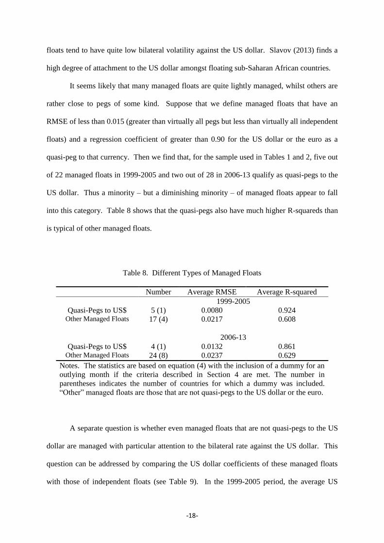
It seems likely that many managed floats are quite lightly managed, whilst others are

rather close to pegs of some kind. Suppose that we define managed floats that have an

RMSE of less than 0.015 (greater than virtually all pegs but less than virtually all independent

floats) and a regression coefficient of greater than 0.90 for the US dollar or the euro as a

quasi-peg to that currency. Then we find that, for the sample used in Tables 1 and 2, five out

of 22 managed floats in 1999-2005 and two out of 28 in 2006-13 qualify as quasi-pegs to the

US dollar. Thus a minority – but a diminishing minority – of managed floats appear to fall

into this category. Table 8 shows that the quasi-pegs also have much higher R-squareds than

is typical of other managed floats.

Table 8. Different Types of Managed Floats

Number Average RMSE Average R-squared

1999-2005

Quasi-Pegs to US$ 5 (1) 0.0080 0.924 Other Managed Floats 17 (4) 0.0217 0.608

2006-13

Quasi-Pegs to US$ 4 (1) 0.0132 0.861 Other Managed Floats 24 (8) 0.0237 0.629

Notes. The statistics are based on equation (4) with the inclusion of a dummy for an

outlying month if the criteria described in Section 4 are met. The number in

parentheses indicates the number of countries for which a dummy was included.

“Other” managed floats are those that are not quasi-pegs to the US dollar or the euro.

A separate question is whether even managed floats that are not quasi-pegs to the US

dollar are managed with particular attention to the bilateral rate against the US dollar. This

question can be addressed by comparing the US dollar coefficients of these managed floats

with those of independent floats (see Table 9). In the 1999-2005 period, the average US

-19-

dollar coefficient of “other” managed floats is 0.781, which is slightly higher than the average

of 0.697 for independent floats. In 2006-13, the average US dollar coefficient of “other”

managed floats is still quite high, at 0.686, wheareas the average for independent floats is

much lower, at 0.205. The euro coefficients are very similar across the two periods for each

group (0.315 and 0.347 for “other” managed floats; 0.700 and 0.720 for independent floats),

but much lower for independent floats. Of course geographical factors may be involved here,

as we investigate below.

The bottom panel of Table 9 shows the average coefficients for the seven currencies

that were independent floats in the IMF de facto classification throughout the 1999-2013

period. The difference between the US dollar coefficients in the two periods is now much

smaller, but a large difference now appears between the euro coefficients in the two periods.

Considerable volatility in the coefficients of equation (4) is to be expected for genuinely

floating countries.

Table 9. Average US$ and Euro Coefficients of Different Types of Floats

Number Average US$

coefficient

Average euro

coefficient

1999-2005

Quasi-Pegs to US$ 5 (1) 0.997 0.040 Other Managed Floats 17 (4) 0.781 0.315

Independent Floats 15 (0) 0.697 0.700

2006-13

Quasi-Pegs to US$ 4 (1) 0.919 0.091 Other Managed Floats 24 (8) 0.668 0.340

Independent Floats 10 (2) 0.187 0.680 Statistics for the same seven independent floats

1999-2005 7 (0) 0.51 0.93 2006-13 7 (1) 0.32 0.50

Notes. See notes to Table 8. The seven countries in the bottom panel are: Australia,

Canada, Chile, Japan, New Zealand, Sweden and the United Kingdom.

-20-

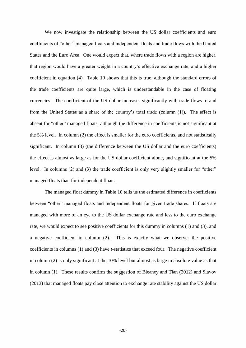
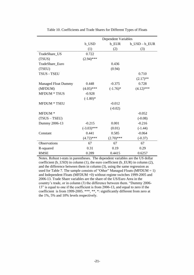
We now investigate the relationship between the US dollar coefficients and euro

coefficients of “other” managed floats and independent floats and trade flows with the United

States and the Euro Area. One would expect that, where trade flows with a region are higher,

that region would have a greater weight in a country’s effective exchange rate, and a higher

coefficient in equation (4). Table 10 shows that this is true, although the standard errors of

the trade coefficients are quite large, which is understandable in the case of floating

currencies. The coefficient of the US dollar increases significantly with trade flows to and

from the United States as a share of the country’s total trade (column (1)). The effect is

absent for “other” managed floats, although the difference in coefficients is not significant at

the 5% level. In column (2) the effect is smaller for the euro coefficients, and not statistically

significant. In column (3) (the difference between the US dollar and the euro coefficients)

the effect is almost as large as for the US dollar coefficient alone, and significant at the 5%

level. In columns (2) and (3) the trade coefficient is only very slightly smaller for “other”

managed floats than for independent floats.

The managed float dummy in Table 10 tells us the estimated difference in coefficients

between “other” managed floats and independent floats for given trade shares. If floats are

managed with more of an eye to the US dollar exchange rate and less to the euro exchange

rate, we would expect to see positive coefficients for this dummy in columns (1) and (3), and

a negative coefficient in column (2). This is exactly what we observe: the positive

coefficients in columns (1) and (3) have t-statistics that exceed four. The negative coefficient

in column (2) is only significant at the 10% level but almost as large in absolute value as that

in column (1). These results confirm the suggestion of Bleaney and Tian (2012) and Slavov

(2013) that managed floats pay close attention to exchange rate stability against the US dollar.

-21-

Table 10. Coefficients and Trade Shares for Different Types of Floats

Dependent Variables

b_USD b_EUR b_USD – b_EUR

(1) (2) (3)

TradeShare_US 0.722

(TSUS) (2.94)***

TradeShare_Euro

0.436

(TSEU)

(0.94)

TSUS - TSEU 0.710

(2.17)**

Managed Float Dummy 0.448 -0.375 0.728

(MFDUM) (4.05)*** (-1.76)* (4.12)***

MFDUM * TSUS -0.928

(-1.80)*

MFDUM * TSEU

-0.012

(-0.02)

MFDUM * -0.052

(TSUS – TSEU) (-0.08)

Dummy 2006-13 -0.215 0.001 -0.216

(-3.03)*** (0.01) (-1.44)

Constant 0.441 0.585 -0.064

(4.72)*** (2.70)*** (-0.37)

Observations 67 67 67

R-squared 0.31 0.19 0.29

RMSE 0.289 0.4415 0.6257

Notes. Robust t-stats in parentheses. The dependent variables are the US dollar

coefficient (b_USD) in column (1), the euro coefficient (b_EUR) in column (2),

and the difference between them in column (3), using the same regression as

used for Table 7. The sample consists of “Other” Managed Floats (MFDUM = 1)

and Independent Floats (MFDUM =0) without regime switches 1999-2005 and

2006-13. Trade Share variables are the share of the US/Euro Area in the

country’s trade, or in column (3) the difference between them. “Dummy 2006-

13” is equal to one if the coefficient is from 2006-13, and equal to zero if the

coefficient is from 1999-2005. ***, **, *: significantly different from zero at

the 1%, 5% and 10% levels respectively.

-22-

8 Generating an Annual Classification

It is often useful to have an annual classification of exchange rate regimes, in order to assess

how macroeconomic variables such as growth, inflation and fiscal balances vary across

regimes, to capture trends in regime choice over time, or simply to provide a comparison with

earlier classification schemes that are organized by calendar year. The main issue for any

regression method applied to a relatively short period is the loss of degrees of freedom.

Applied to twelve monthly changes, equation (4) would have only nine degrees of freedom

(fewer if extra potential anchor currencies are included), and only eight once a parity change

in one month is allowed for.

In order to generate an annual classification for each country-year observation, we

adopt the following algorithm.

1) Estimate equation (4) for the twelve monthly exchange rate changes in the year,

adding potential anchor currencies to the US dollar and the euro as appropriate. If the

RMSE ≤ 0.01, define that country-year observation as a PEG; if the RMSE > 0.01, go

to step 2.

2) Add a dummy for January to the regression, then replace that with a dummy for

February, and so on. If the RMSE ≤ 0.01 in any of these twelve regressions, define

that country-year observation as a PEG WITH A PARITY CHANGE; otherwise

define it as a FLOAT.

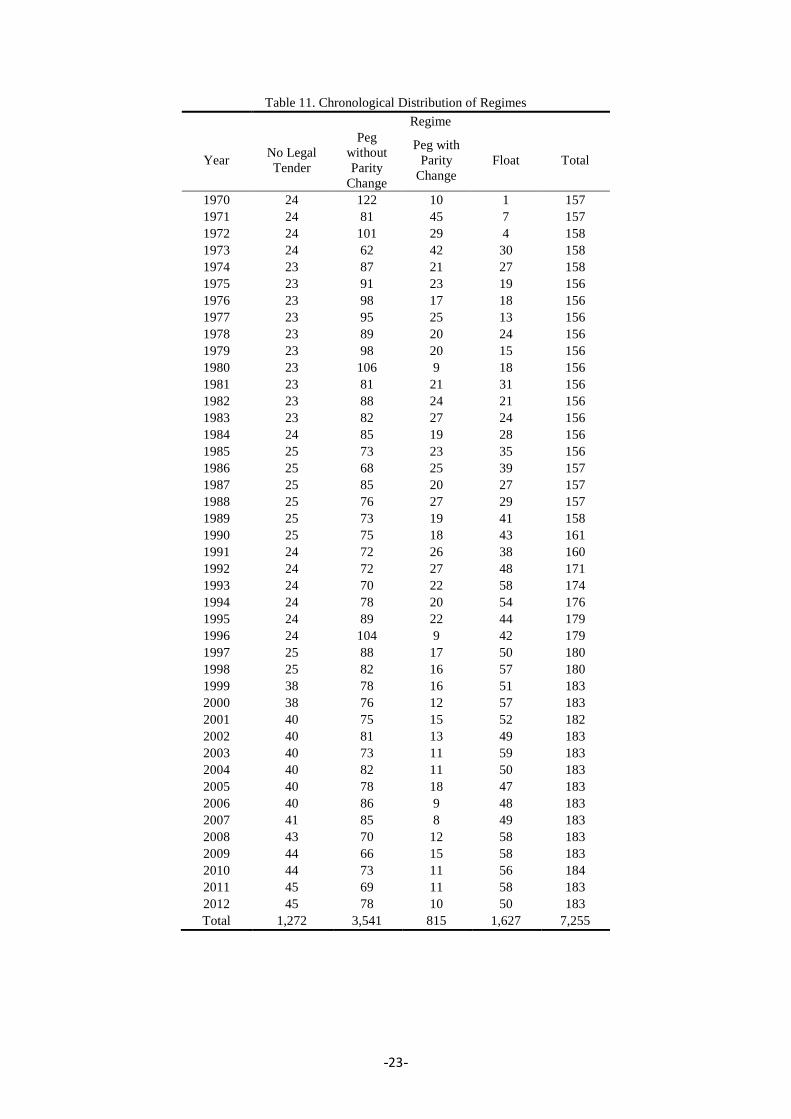
Table 11 gives the number of countries in each of these categories, plus those with no

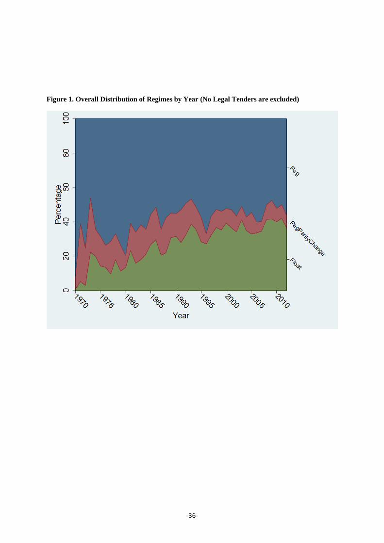
separate legal tender, in every year from 1970 to 2012. The number of countries with no

separate legal tender has increased to nearly 25% of the total. Floats increased up to the

1990s, but not since. Pegs with parity changes have decreased as inflation rates have

declined; pegs without parity changes remain the most frequent category, but with some

tendency to decline.

-23-

Table 11. Chronological Distribution of Regimes

Regime

Year No Legal

Tender

Peg

without

Parity

Change

Peg with

Parity

Change

Float Total

1970 24 122 10 1 157

1971 24 81 45 7 157

1972 24 101 29 4 158

1973 24 62 42 30 158

1974 23 87 21 27 158

1975 23 91 23 19 156

1976 23 98 17 18 156

1977 23 95 25 13 156

1978 23 89 20 24 156

1979 23 98 20 15 156

1980 23 106 9 18 156

1981 23 81 21 31 156

1982 23 88 24 21 156

1983 23 82 27 24 156

1984 24 85 19 28 156

1985 25 73 23 35 156

1986 25 68 25 39 157

1987 25 85 20 27 157

1988 25 76 27 29 157

1989 25 73 19 41 158

1990 25 75 18 43 161

1991 24 72 26 38 160

1992 24 72 27 48 171

1993 24 70 22 58 174

1994 24 78 20 54 176

1995 24 89 22 44 179

1996 24 104 9 42 179

1997 25 88 17 50 180

1998 25 82 16 57 180

1999 38 78 16 51 183

2000 38 76 12 57 183

2001 40 75 15 52 182

2002 40 81 13 49 183

2003 40 73 11 59 183

2004 40 82 11 50 183

2005 40 78 18 47 183

2006 40 86 9 48 183

2007 41 85 8 49 183

2008 43 70 12 58 183

2009 44 66 15 58 183

2010 44 73 11 56 184

2011 45 69 11 58 183

2012 45 78 10 50 183

Total 1,272 3,541 815 1,627 7,255

-24-

Figure 1 shows the number of floats and pegs with and without parity changes as a

share of all currencies (i.e. countries with a separate legal tender). Floats have increased to

about 40% of the total in recent years, at the expense of pegs both with and without parity

changes.4

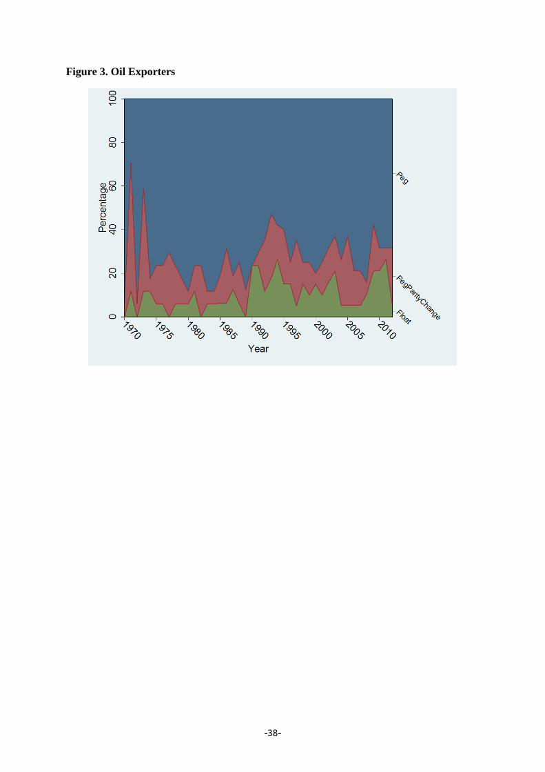
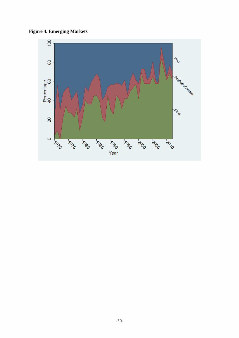
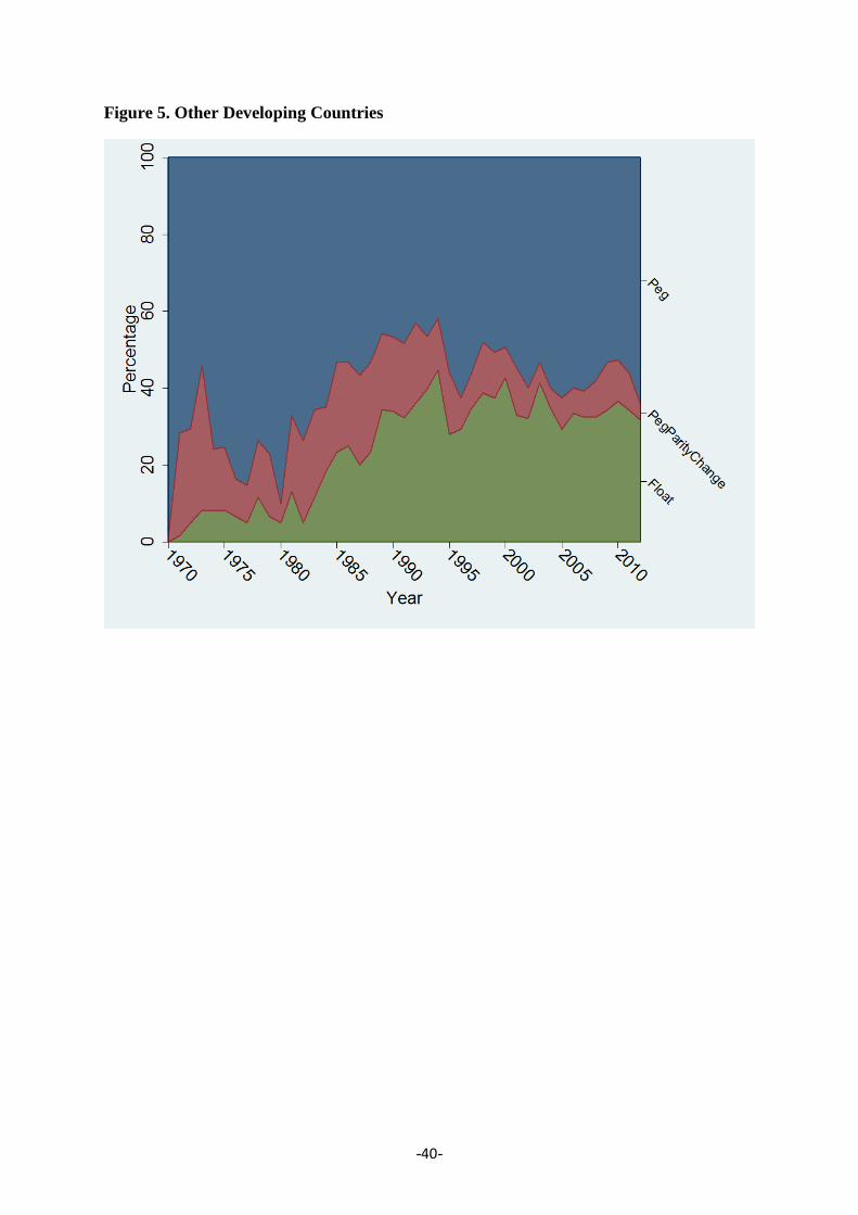
When we disaggregate Figure 1 by type of country, it is clear that oil exporters and

offshore financial centres remain wedded to pegs (Figures 2 and 3), whilst emerging markets

have exhibited a steady trend towards floating (Figure 4). Other developing countries were

shifting towards floating up to the mid-1990s, but that trend has stopped since, without being

significantly reversed (Figure 5).

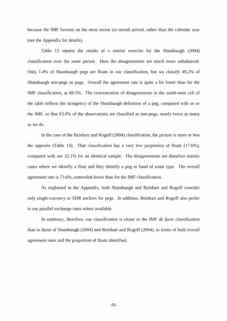
How does our annual classification compare with others? Table 12 shows a summary

comparison of our classification with the IMF’s de facto classification for the years 1980-

2011. The comparison is based on currencies rather than countries (i.e. the CFA franc, for

example, is counted only once for each year). Overall, we identify 33.4% of the observations

as floats compared with the IMF’s 36.9%, which is quite a close match. The difference arises

mainly because we categorise 44.4% of IMF managed floats as pegs, and that is not fully

compensated for by the proportion of IMF pegs and bands that we classify as floats (5.2% for

conventional pegs, 17.7% for basket pegs, 23.6% for bands and 32.6% for crawls). Our

overall agreement rate with the IMF classification is 77.0%.

Our disagreements with the IMF classification are difficult to evaluate. Even if

managed floats are not in reality quasi-pegs (and some are, as our previous analysis showed),

they might be quite tightly managed for limited periods, and therefore show up in our annual

classification as a peg in some years. Likewise, bands and crawls may have a wider range of

fluctuation in some years, and appear in our analysis as floats. Some discrepancies can arise

4 Our annual regime classifications are publicly available at

http://www.nottingham.ac.uk/economics/people/michael.bleaney.

-25-

because the IMF focuses on the most recent six-month period, rather than the calendar year

(see the Appendix for details).

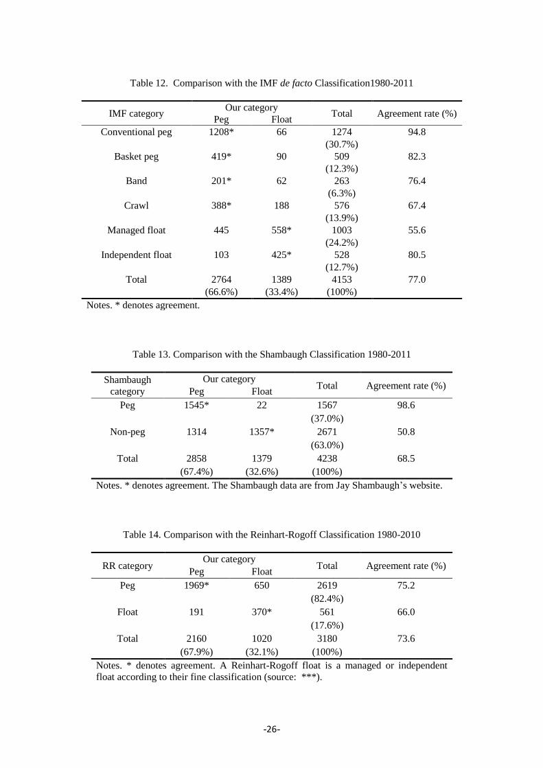
Table 13 reports the results of a similar exercise for the Shambaugh (2004)

classification over the same period. Here the disagreements are much more unbalanced.

Only 1.4% of Shambaugh pegs are floats in our classification, but we classify 49.2% of

Shambaugh non-pegs as pegs. Overall the agreement rate is quite a bit lower than for the

IMF classification, at 68.5%. The concentration of disagreements in the south-west cell of

the table reflects the stringency of the Shambaugh definition of a peg, compared with us or

the IMF, so that 63.0% of the observations are classified as non-pegs, nearly twice as many

as we do.

In the case of the Reinhart and Rogoff (2004) classification, the picture is more or less

the opposite (Table 14). That classification has a very low proportion of floats (17.6%),

compared with our 32.1% for an identical sample. The disagreements are therefore mainly

cases where we identify a float and they identify a peg or band of some type. The overall

agreement rate is 73.6%, somewhat lower than for the IMF classification.

As explained in the Appendix, both Shambaugh and Reinhart and Rogoff consider

only single-currency or SDR anchors for pegs. In addition, Reinhart and Rogoff also prefer

to use parallel exchange rates where available.

In summary, therefore, our classification is closer to the IMF de facto classification

than to those of Shambaugh (2004) and Reinhart and Rogoff (2004), in terms of both overall

agreement rates and the proportion of floats identified.

-26-

Table 12. Comparison with the IMF de facto Classification1980-2011

IMF category Our category

Total Agreement rate (%) Peg Float

Conventional peg 1208* 66 1274 94.8

(30.7%)

Basket peg 419* 90 509 82.3

(12.3%)

Band 201* 62 263 76.4

(6.3%)

Crawl 388* 188 576 67.4

(13.9%)

Managed float 445 558* 1003 55.6

(24.2%)

Independent float 103 425* 528 80.5

(12.7%)

Total 2764 1389 4153 77.0

(66.6%) (33.4%) (100%)

Notes. * denotes agreement.

Table 13. Comparison with the Shambaugh Classification 1980-2011

Shambaugh

category

Our category Total Agreement rate (%)

Peg Float

Peg 1545* 22 1567 98.6

(37.0%)

Non-peg 1314 1357* 2671 50.8

(63.0%)

Total 2858 1379 4238 68.5

(67.4%) (32.6%) (100%)

Notes. * denotes agreement. The Shambaugh data are from Jay Shambaugh’s website.

Table 14. Comparison with the Reinhart-Rogoff Classification 1980-2010

RR category Our category

Total Agreement rate (%) Peg Float

Peg 1969* 650 2619 75.2

(82.4%)

Float 191 370* 561 66.0

(17.6%)

Total 2160 1020 3180 73.6

(67.9%) (32.1%) (100%)

Notes. * denotes agreement. A Reinhart-Rogoff float is a managed or independent

float according to their fine classification (source: ***).

-27-

9 Conclusions

A simple and reliable regression method is used to identify the exchange rate regime. The

method is not data-intensive and could easily be applied by other researchers. Monthly

exchange rate movements of a currency against a floating numéraire currency are regressed

on movements of the euro and the US dollar against the numéraire currency. Where relevant,

other potential anchor currencies are added to the regression. Pegs are characterised by a low

RMSE and a high R-squared, with the estimated coefficients indicating the anchor basket.

Results are robust to the choice of numéraire (except that the SDR tends to be misleading

because of its correlation with the anchor currencies). The thorny question of distinguishing

floats from pegs with occasional parity changes can be addressed by examining the skewness

of residuals; floats have relatively symmetric residuals whereas pegs with occasional parity

changes do not. The procedure can be repeated with outlying observations dummied out to

distinguish pegs with parity changes from genuine floats. A useful by-product of this

procedure is that it also distinguishes “fixed” pegs (those without parity changes) from

“variable” pegs (those with parity changes).

Managed floats have become increasingly popular amongst emerging markets and

developing countries in the 21st century. In a small but diminishing minority of cases, our

results show that these are quasi-pegs to the US dollar, often with slightly wider target zones

than announced pegs. An increasing proportion of managed floats has similar volatility to

independent floats, but even these have a tendency to track the US dollar.

The method can be used to generate an annual classification. It could also be used by

the IMF’s Monetary and Exchange Affairs Department (or country desks themselves) to

verify country desks’ identification of the exchange rate regime. The simple criterion of

-28-

RMSE > or < 0.01 in twelve-month data, after allowing for a possible parity change, yields a

reasonably high correlation with the IMF de facto classification. The agreement rate of our

system with alternative classification schemes, such as those of Shambaugh (2004) or

Reinhart and Rogoff (2004), is lower than with the IMF de facto classification. In particular,

our estimate of the overall frequency of floating is much closer to that of the IMF than of the

alternatives. Thus our approach may be regarded as providing a solid statistical foundation

for the IMF de facto classification.

References

Bénassy-Quéré, A., B. Coeuré and V. Mignon (2006), On the identification of de facto

currency pegs, Journal of the Japanese and International Economies 20, 112-127

Bleaney, M.F. and M. Francisco (2007), Classifying exchange rate regimes: a statistical

analysis of alternative methods, Economics Bulletin 6 (3), 1-6.

Bleaney, M.F. and M. Tian (2012), Currency networks, bilateral exchange rate volatility and

the role of the US dollar, Open Economies Review 23 (5), 785-803

Calvo, G. and C.M. Reinhart (2002), Fear of floating, Quarterly Journal of Economics 117

(2), 379-408

Frankel, J. and S.-J. Wei (1995), Emerging currency blocs, in The International Monetary

System: Its Institutions and its Future, ed. H. Genberg (Berlin, Springer)

Frankel, J. and S.-J. Wei (2008), Estimation of de facto exchange rate regimes: synthesis of

the techniques for inferring flexibility and basket weights, IMF Staff Papers 55 (3), 384-416

Habermeier, K., A. Kokenyne, R. Veyrune and H. Anderson (2009), Revised system for the

classification of exchange rate arrangements, IMF Working Paper no. 09/211

Levy-Yeyati, E. and F. Sturzenegger (2005), Classifying exchange rate regimes: deeds versus

words, European Economic Review 49 (6), 1173-1193

Reinhart, C.M. and Rogoff, K. (2004), The modern history of exchange rate arrangements: a

re-interpretation, Quarterly Journal of Economics 119 (1), 1-48

Shambaugh, J. (2004), The effects of fixed exchange rates on monetary policy, Quarterly

Journal of Economics 119 (1), 301-352

-29-

Slavov, S.T. (2013), De jure versus de facto exchange rate regimes in sub-Saharan Africa,

Journal of African Economies 22 (5), 732-756

Tavlas, G., H. Dellas and A.C. Stockman (2008), The classification and performance of

alternative exchange-rate systems, European Economic Review 52, 941-963

-30-

Appendix

10 Summaries of Classification Schemes

10.1 IMF Classification

The de facto classification is based on the ex post evaluation of each country’s report (de jure

classification) against the expected behaviour of some selective measures usually for at least six

months. If these ex post measures disagree with the de jure classification, the country will be re-

classified into the actual category. Detailed criteria for each category are summarised as follows:

No Separate Legal Tender and Currency Board: These regimes are usually defined explicitly by

country’s exchange rate policy.

Conventional Pegs / Stabilised Arrangement: The spot market rate vis-à-vis the anchor(s)

fluctuates within ±1% around a central rate or within a 2% margin for at least six months,

allowing for some occasional outliers as exceptions. The anchor(s), usually reflecting the major

trade partners in goods, services, and capitals, would be verified by statistical techniques (the

details are not given).

Crawls/Crawl-like Arrangement: The exchange rate fluctuates within a margin about a

predetermined trend (identified by using ``statistical methods’’): either around a time trend for at

least six months with the overall changes larger than 2% or within the boundary created by ex

post/projected inflation differentials against the country’s major trading partners, or it exhibits

seemingly single-side changes with the annual size larger than 1%.

Pegged within Horizontal Bands: The exchange rate fluctuates around a central rate greater than

±1% or exceeding the 2% max-min margin, but within a certain margin (upper boundary not

specified).

Managed Floating: Those currencies do not satisfy any of the other categories (usually for those

with frequent policy shifts) or exhibit some managing behaviours by using some ``broadly-

judgemental’’ indicators (e.g. balance of payment position, international reserves, parallel market

developments). Since 2009 this category has been split into “Floats” and “Other Managed

Arrangements”.

Free/Independent Floating: Either the authority provides information that the exchange rate

interventions only aims to ``address disorderly market conditions’’, or data can confirm that

within the previous six months there are no more than three interventions with each lasting less

than three business days.

10.2 Reinhart and Rogoff’s Classification

Reinhart and Rogoff’s classification method also embeds a statistical de jure verification procedure,

but this is conditioned upon the non-existence of the parallel exchange rate market rates. If the

parallel rates are available, they will be directly evaluated to generate the classification result. The

verification/evaluation procedure generally employs the mean absolute percentage changes of

monthly exchange rates mainly over a 5-year rolling-window (if not, a 2-year window instead),

accompanied by inflation data and various sources of documents. The potential anchors are chosen

either based on the authority’s pre-announcement, or from a basket proxied by a single dominant

currency or the SDR. Detailed criteria for each category are summarised as follows:

-31-

Pegs/Crawling/Moving Pegs: The mean absolute percentage changes of exchange rates stay zero

for more than 4 months, or within a ±1% band for more than 80% of cases over the 5-year rolling

window

Bands/Crawling/Moving Bands: The mean absolute percentage changes of exchange rates stays

within ±5% band for more than 80% cases over the 5-year rolling window.

Freely Falling/Hyperfloat: Those failed to be classified as a peg and exhibiting a 12-month

inflation higher than 40% (Freely Falling) or further has a single month inflation larger than 40%

(Hyperfloat)

Managed Float/Free Floating: The residuals from the above categories. Based on the empirical

distribution of the ratio defined as the 5-year mean absolute percentage changes of exchange

rates to the proportion of the cases within ±1% band, a Free Float episode lies in the 99 percent

upper tail of the distribution of the floater’s group.

10.3 Shambaugh’s Classification

Shambaugh’s dichotomy classification mainly investigates the currency’s official end-of-month

bilateral exchange rates against a single anchor within a calendar year. The anchor is chosen by

utilising historical documents as well as by examining the bilateral exchange rates against all global

and regional major currencies to identify the potential pegging behaviours. Detailed criteria for each

category are summarised as follows:

Pegs: The exchange rate fluctuates within a ±2% band throughout the entire year or there are 11

months zero changes.

Non-Pegs: Those that do not satisfy the criteria for Pegs.

10.4 Our Regression Method

Our annual classification is based on a regression using the log-changes of the currency value on a

potential anchor basket of currencies, all measured in terms of a common numeraire (the end-of-

month official exchange rates against CHF). See Section 2 for the anchor list. Our data covers the

period 1970-2012 and a currency-year list is presented in Section 3.

An outlier month dummy is introduced and tested each throughout the year to capture one-time parity

change. A month dummy is accepted if its t-statistics in magnitude is the larger than those for the

other months tests and is above 5.48 (equivalent to 30 for the F-statistics), in which the episode is

coded as Peg with Parity Change.

For the residual episodes, a Peg is coded if the rooted mean square error of the regression is smaller

than 1%. Otherwise it is regarded as a Float.

A separate No Legal Tender category is constructed, based on various documents and listed in Section

3.

-32-

11 Potential Anchor List Introduced in the Regression

11.1 The following anchors are added in the regressions until 1998

DEM

All Currencies except those having FRF

FRF:

Benin, Burkina Faso, CAEMU, Cameroon, Central African Republic, Chad, Comoros, Congo,

Cote d'Ivoire, Equatorial Guinea, Gabon, Guinea, Guinea-Bissau, Madagascar, Mali, Mauritania,

Niger, Senegal, Togo, WAEMU

GBP:

Anguilla, Antigua and Barbuda, Australia, Bahamas, Bahrain, Bangladesh, Barbados, Belize,

Botswana, Brunei, Cyprus, Dominica, Egypt, Fiji, Gambia, Ghana, Grenada, Guyana, Hong

Kong, Iceland, India, Iraq, Ireland, Israel, Jamaica, Jordan, Kenya, Kiribati, Kuwait, Lesotho,

Libya, Malawi, Malaysia, Maldives, Malta, Mauritius, Montserrat, Namibia, New Zealand,

Oman, Pakistan, Papua New Guinea, Qatar, Saint Kitts and Nevis, Saint Lucia, Saint Vincent and

the Grenadines, Samoa, Seychelles, Sierra Leone, Singapore, Solomon Islands, Somalia, South

Africa, Sri Lanka, Sudan, Swaziland, Tonga, Trinidad and Tobago, Uganda, United Arab

Emirates, Zambia

PTE

Angola, Cape Verde, Guinea-Bissau, Mozambique, Sao Tome and Principe

ITL

Albania, San Marino

BEF

Luxembourg

11.2 The following anchors are added from 1999

EUR

All currencies

11.3 The following anchors are added throughout the sample period

USD

All currencies

AUD

Fiji, Kiribati, Papua New Guinea, Samoa, Solomon Islands, Tonga, Vanuatu

NZD

Fiji, Kiribati, Papua New Guinea, Samoa, Solomon Islands, Tonga, Vanuatu

ZAR

Botswana, Lesotho, Namibia, Swaziland

INR

Bangladesh, Bhutan, Maldives, Nepal, Pakistan, Seychelles, Sri Lanka

SGD

Brunei

-33-

11.4 The regimes for the following currencies are underdetermined

USD SWF EUR FRF DEM

12 No Legal Tender Espisodes

Table. No Legal Tender

Name Period Name Period

Anguilla 1970-2012 Kiribati 1970-2012

Antigua and Barbuda 1970-2012 Luxembourg 1999-2012

Austria 1999-2012 Mali 1984-2012

Belgium 1999-2012 Malta 2008-2012

Benin 1970-2012 Mauritania 1970-1973

Burkina Faso 1970-2012 Micronesia 1970-2012

Cameroon 1970-2012 Montenegro 1999-2012

Central African Republic 1970-2012 Montserrat 1970-2012

Chad 1970-2012 Namibia 1970-1990

Congo 1970-2012 Netherlands 1999-2012

Cote d'Ivoire 1970-2012 Niger 1970-2012

Cyprus 2008-2012 Panama 1970-2012

Dominica 1970-2012 Portugal 1999-2012

El Salvador 2001-2012 Saint Kitts and Nevis 1970-2012

Equatorial Guinea 1985-2012 Saint Lucia 1970-2012

Estonia 2011-2012 Saint Vincent and the

Grenadines 1970-2012

Finland 1999-2012 San Marino 1999-2012

Gabon 1970-2012 Senegal 1970-2012

Greece 2001-2012 Slovak Republic 2009-2012

Grenada 1970-2012 Slovenia 2007-2012

Guinea-Bissau 1997-2012 Spain 1999-2012

Ireland 1999-2012 Togo 1970-2012

Italy 1999-2012

13 Country Year List

Table. Currency Year List

Name Period Name Period

Industrial

Financial

Australia 1970-2012 Aruba 1986-2012

Austria 1970-1998 Bahamas 1970-2012

Belgium 1970-1998 Barbados 1970-2012

Canada 1970-2012 Belize 1970-2012

Denmark 1970-2012 Cyprus 1970-2007

Finland 1970-1998 Hong Kong 1970-2012

Greece 1970-2000 Lebanon 1970-2012

-34-

Iceland 1970-2012 Macao 1970-2012

Ireland 1970-1998 Malta 1970-2007

Italy 1970-1998 Mauritius 1970-2012

Japan 1970-2012 Netherlands Antilles 1970-2010

Luxembourg 1970-1998 Samoa 1970-2012

Netherlands 1970-1998 Singapore 1970-2012

New Zealand 1970-2012 Vanuatu 1970-2012

Norway 1970-2012

Portugal 1970-1998 Emerging Market

San Marino 1970-1998 Argentina 1970-2012

Spain 1970-1998 Brazil 1970-2012

Sweden 1970-2012 Bulgaria 1970-1974

1990-2012

United Kingdom 1970-2012 Chile 1970-2012

China 1970-2012

Fuel

Colombia 1970-2012

Algeria 1970-2012 Czech Republic 1993-2012

Angola 1970-2012 Egypt 1970-2012

Azerbaijan 1995-2012 Hungary 1970-2012

Bahrain 1970-2012 India 1970-2012

Brunei 1970-2012 Indonesia 1970-2012

Equatorial Guinea 1970-1984 Israel 1970-2012

Iran 1970-2012 Malaysia 1970-2012

Iraq 1970-2012 Mexico 1970-2012

Kazakhstan 1994-2012 Morocco 1970-2012

Kuwait 1970-2012 Pakistan 1970-2012

Libya 1970-2012 Peru 1970-2012

Nigeria 1970-2012 Philippines 1970-2012

Oman 1970-2012 Poland 1970-2012

Qatar 1970-2012 Russia 1992-1993

1995-2012

Saudi Arabia 1970-2012 South Africa 1970-2012

Sudan 1970-2012 South Korea 1970-2012

Trinidad and Tobago 1970-2012 Thailand 1970-2012

Turkmenistan 1994-2001 Turkey 1970-2012

United Arab Emirates 1970-2012 Ukraine 1993-2012

Venezuela 1970-2012 Uruguay 1970-2012

Yemen Arab Republic 1990-2012

Other Developing

Afghanistan 1970-1998

2002-2012 Liberia 1970-2012

Albania 1992-2012 Lithuania 1992-2012

Armenia 1992-2012 Macedonia 1994-2012

Bangladesh 1972-2012 Madagascar 1970-2012

Belarus 1992-2012 Malawi 1970-2012

-35-

Bhutan 1970-2012 Maldives 1970-2012

Bolivia 1970-2012 Mali 1970-1983

Bosnia and Herzegovina 1997-2012 Mauritania 1974-2012

Botswana 1970-2012 Moldova 1992-2012

Burundi 1970-2012 Mongolia 1990-2012

CAEMU 1970-2012 Mozambique 1970-2012

Cambodia 1970-1974

1989-2012 Myanmar 1970-2012

Cape Verde 1970-2012 Namibia 1991-2012

Comoros 1970-2012 Nepal 1970-2012

Costa Rica 1970-2012 Nicaragua 1970-2012

Croatia 1992-2012 Papua New Guinea 1970-2012

Democratic Republic of

Congo 1970-2012 Paraguay 1970-2012

Djibouti 1970-2012 Romania 1970-2012

Dominican Republic 1970-2012 Rwanda 1970-2012

ECD 1970-2012 Sao Tome and Principe 1970-2012

El Salvador 1970-2000 Seychelles 1970-2012

Eritrea 1970-2012 SerbiaRep 2002-2012

Estonia 1992-2010 Sierra Leone 1970-2012

Ethiopia 1970-2012 SintMaarten 2010-2012

Fiji 1970-2012 Slovak Republic 1993-2008

Gambia 1970-2012 Slovenia 1992-2006

Georgia 1995-2012 Solomon Islands 1970-2012

Ghana 1970-2012 Somalia 1970-1990

Guatemala 1970-2012 Sri Lanka 1970-2012

Guinea 1970-2012 Suriname 1970-2012

Guinea-Bissau 1970-1996 Swaziland 1970-2012

Guyana 1970-2012 Tajikistan 1992-2012

Haiti 1970-2012 Tanzania 1970-2012

Honduras 1970-2012 Tonga 1970-2012

Jamaica 1970-2012 Tunisia 1970-2012

Jordan 1970-2012 Uganda 1970-2012

Kenya 1970-2012 Uzbekistan 1999-2000

Kyrgyz Republic 1993-2012 Vietnam 1970-2012

Laos 1970-2012 WAEMU 1970-2012

Latvia 1992-2012 Yugoslavia 1970-1992

Lesotho 1970-2012 Zambia 1970-2012

-36-

Figure 1. Overall Distribution of Regimes by Year (No Legal Tenders are excluded)

-37-

Figure 2. Offshore Financial Centres

-38-

Figure 3. Oil Exporters

-39-

Figure 4. Emerging Markets

-40-

Figure 5. Other Developing Countries