classification of variables

b a c k n e x th o m e

Classification of Variables

Discrete Numerical VariableDiscrete Numerical VariableA variable that produces a response that comes from a counting process.



Continuous Numerical VariableContinuous Numerical VariableA variable that produces a response that is the outcome of a measurement process.



Categorical VariablesCategorical VariablesVariables that produce responses that belong to groups (sometimes called “classes”) or categories.


Measurement Levels

NominalNominal and OrdinalOrdinal Levels of Measurement refer to data obtained from categorical questions.

• A nominal scale indicates assignments to groups or classes.

• Ordinal data indicate rank ordering of items.


Frequency Distributions

A frequency distributionfrequency distribution is a table used to organize data. The left column (called classes or groups) includes numerical intervals on a variable being studied. The right column is a list of the frequencies, or number of observations, for each class. Intervals are normally of equal size, must cover the range of the sample observations, and be non-overlapping.


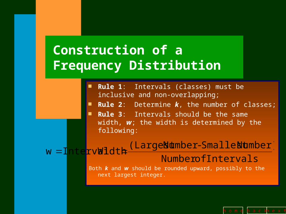
Construction of a Frequency Distribution

Rule 1: Intervals (classes) must be inclusive and non-overlapping;

Rule 2: Determine k, the number of classes; Rule 3: Intervals should be the same width, w;

the width is determined by the following:

Both k and w should be rounded upward, possibly to the next largest integer.

Intervals ofNumber

Number)Smallest -Number (Largest Width Interval w


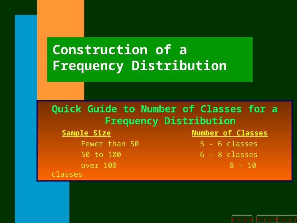
Construction of a Frequency Distribution

Quick Guide to Number of Classes for a Frequency Distribution

Sample Size Number of Classes

Fewer than 50 5 – 6 classes

50 to 100 6 – 8 classes

over 100 8 – 10 classes


Cumulative Frequency Distributions

A cumulative frequency distributioncumulative frequency distribution contains the number of observations whose values are less than the upper limit of each interval. It is constructed by adding the frequencies of all frequency distribution intervals up to and including the present interval.


Relative Cumulative Frequency Distributions

A relative cumulative frequency relative cumulative frequency distributiondistribution converts all cumulative frequencies to cumulative percentages


Histograms and Ogives

A histogramhistogram is a bar graph that consists of vertical bars constructed on a horizontal line that is marked off with intervals for the variable being displayed. The intervals correspond to those in a frequency distribution table. The height of each bar is proportional to the number of observations in that interval.


Histograms and Ogives

An ogiveogive,, sometimes called a cumulative line graph, is a line that connects points that are the cumulative percentage of observations below the upper limit of each class in a cumulative frequency distribution.


Histogram and Ogive for Example 2.1

Histogram of Weights for Example 2.1

0

5

10

15

20

25

30

35

40

224.5 229.5 234.5 239.5 244.5 249.5

Interval Weights (mL)

Fre

qu

ency

0

10

20

30

40

50

60

70

80

90

100


Stem-and-Leaf Display

A stem-and-leaf displaystem-and-leaf display is an exploratory data analysis graph that is an alternative to the histogram. Data are grouped according to their leading digits (called the stem) while listing the final digits (called leaves) separately for each member of a class. The leaves are displayed individually in ascending order after each of the stems.




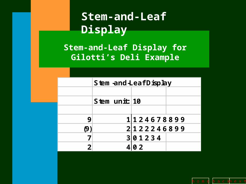
Stem unit: 10

9 1 1 2 4 6 7 8 8 9 9(9) 2 1 2 2 2 4 6 8 9 9

7 3 0 1 2 3 42 4 0 2

Stem-and-Leaf Display for Gilotti’s Deli Example


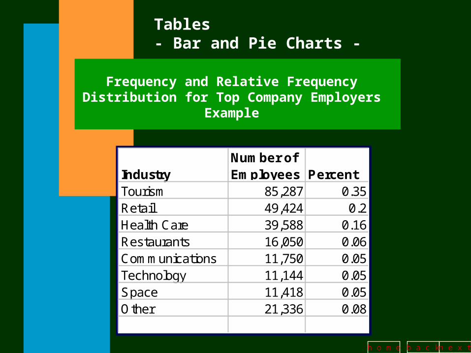
Tables- Bar and Pie Charts -

IndustryNumber ofEmployees Percent

Tourism 85,287 0.35Retail 49,424 0.2Health Care 39,588 0.16Restaurants 16,050 0.06Communications 11,750 0.05Technology 11,144 0.05Space 11,418 0.05Other 21,336 0.08

Frequency and Relative Frequency Distribution for Top Company Employers Example



1999 Top Company Employers in Central Florida

0.35

0.20.16

0.06 0.05 0.05 0.05 0.08

Touris

mReta

il

Health C

are

Restaur

ants

Communic

ation

s

Techn

ology

Space

Other

Industry Category

Figure 2.9 Bar Chart for Top Company

Employers Example



Figure 2.10 Pie Chart for Top Company Employers Example

1999 Top Company Employers in Central Florida

Tourism35%

Retail20%

Health Care16%

Others29%


Pareto Diagrams

A Pareto diagramPareto diagram is a bar chart that displays the frequency of defect causes. The bar at the left indicates the most frequent cause and bars to the right indicate causes in decreasing frequency. A Pareto diagramPareto diagram is use to separate the “vital fewvital few” from the “trivial many.trivial many.”


Line Charts

A line chartline chart, , also called a time plottime plot, , is a series of data plotted at various time intervals. Measuring time along the horizontal axis and the numerical quantity of interest along the vertical axis yields a point on the graph for each observation. Joining points adjacent in time by straight lines produces a time plot.


Line Charts

Growth Trends in Internet Use by Age 1997 to 1999

16.520.2

26.331.3 32.7

9.813.8 15.8 17.2 18.5

5 7.511.4 13 14.2

05

101520253035

Apr-9

7

Jul-9

7

Oct-97

Jan-

98

Apr-9

8

Jul-9

8

Oct-98

Jan-

99

Apr-9

9

Jul-9

9

April 1997 to July 1999

Mil

lio

ns

of

Ad

ult

s

Age 18 to 29

Age 30 to 49

Age 50+


Parameters and Statistics

A statisticstatistic is a descriptive measure computed from a sample of data.

A parameterparameter is a descriptive measure computed from an entire population of data.


Measures of Central Tendency- Arithmetic Mean -

The arithmetic meanarithmetic mean of a set of data is the sum of the data values divided by the number of observations.


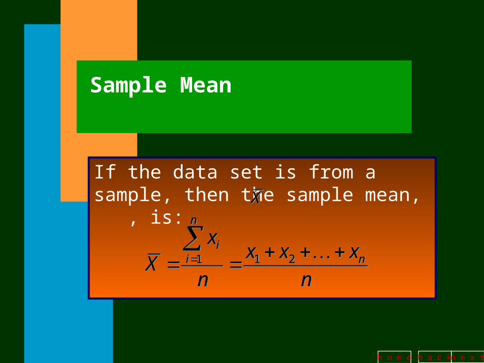
Sample Mean

If the data set is from a sample, then the sample mean, , is:XX

n

xxx

n

xX n

n

ii

211

n

xxx

n

xX n

n

ii

211


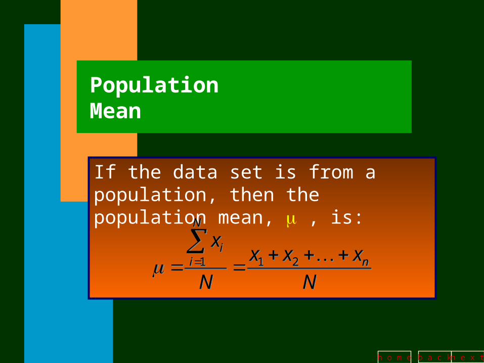
Population Mean

If the data set is from a population, then the population mean, , is:

N

xxx

N

xn

N

ii

211

N

xxx

N

xn

N

ii

211


Measures of Central Tendency- Median -

An ordered arrayordered array is an arrangement of data in either ascending or descending order. Once the data are arranged in ascending order, the medianmedian is the value such that 50% of the observations are smaller and 50% of the observations are larger.


Measures of Central Tendency- Median -

If the sample size n is an odd number, the median, Xm, is the middle observation. If the sample size n is an even number, the medianmedian, Xm, is the average of the two middle observations. The medianmedian will be located in the 0.50(n+1)th ordered position0.50(n+1)th ordered position.


Measures of Central Tendency- Mode -

The modemode, , if one exists, is the most frequently occurring observation in the sample or population.


Shape of the Distribution

The shape of the distribution is said to be symmetricsymmetric if the observations are balanced, or evenly distributed, about the mean. In a symmetric distribution the mean and median are equal.


Shape of the Distribution

A distribution is skewedskewed if the observations are not symmetrically distributed above and below the mean. A positively skewedpositively skewed (or skewed to the right) distribution has a tail that extends to the right in the direction of positive values. A negatively skewednegatively skewed (or skewed to the left) distribution has a tail that extends to the left in the direction of negative values.


Shapes of the Distribution

Symmetric Distribution

0123456789

10

1 2 3 4 5 6 7 8 9

Fre

qu

ency

Positively Skewed Distribution

0

2

4

6

8

10

12

1 2 3 4 5 6 7 8 9

Fre

qu

ency

Negatively Skewed Distribution

0

2

4

6

8

10

12

1 2 3 4 5 6 7 8 9

Fre

qu

ency


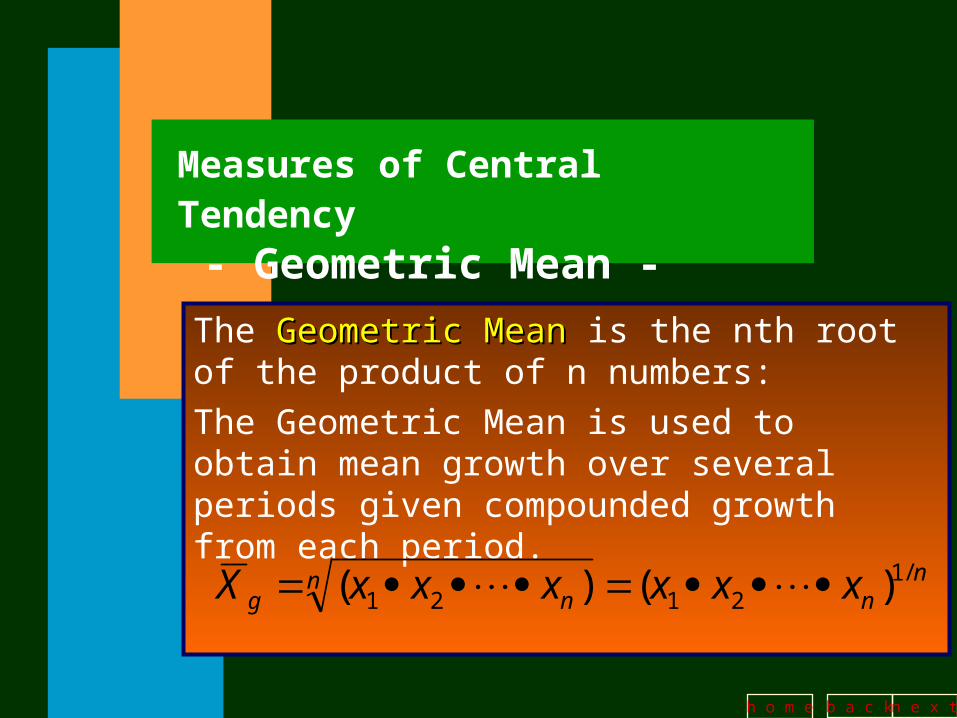
Measures of Central Tendency - Geometric Mean -

The Geometric MeanGeometric Mean is the nth root of the product of n numbers:

The Geometric Mean is used to obtain mean growth over several periods given compounded growth from each period.

nn

nng xxxxxxX /1

2121 )()(


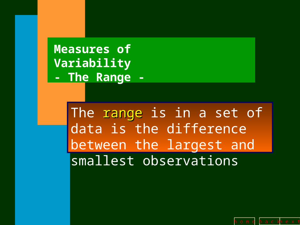
Measures of Variability- The Range -

The rangerange is in a set of data is the difference between the largest and smallest observations


Measures of Variability- Sample Variance -

The sample variance, ssample variance, s22,, is the sum of the squared differences between each observation and the sample mean divided by the sample size minus 1.

1

)(1

2

2

n

Xxs

n

ii


Measures of Variability

- Short-cut Formulas for ss22

Short-cut formulas for the sample variance, ssample variance, s22,, are:

11

)(22

21

2

2

n

Xnxsor

nn

xx

s i

n

i

ii


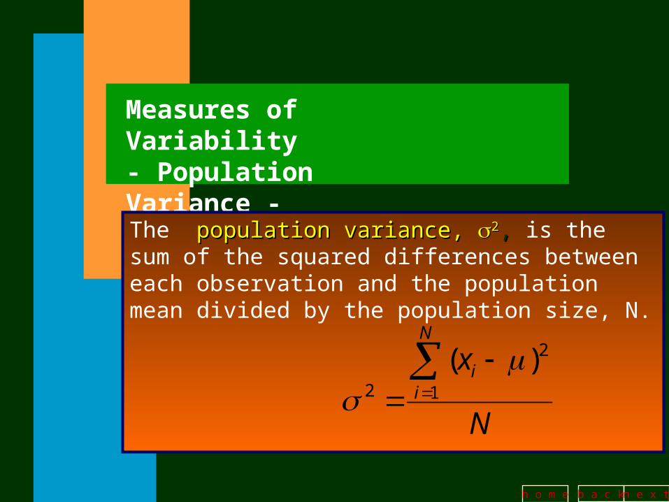
Measures of Variability- Population Variance -

The population variance, population variance, 22, , is the sum of the squared differences between each observation and the population mean divided by the population size, N.

N

xN

ii

1

2

2

)(


Measures of Variability- Sample Standard Deviation -

The sample standard deviation, s,sample standard deviation, s, is the positive square root of the variance, and is defined as:

1

)(1

2

2

n

Xxss

n

ii


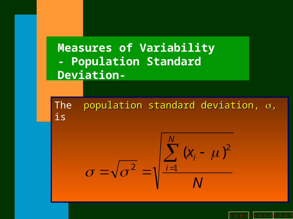
Measures of Variability- Population Standard Deviation-

The population standard deviation, population standard deviation, ,, is

N

xN

ii

1

2

2

)(


The Empirical Rule(the 68%, 95%, or almost all rule)

For a set of data with a mound-shaped histogram, the Empirical RuleEmpirical Rule is:

• approximately 68%68% of the observations are contained with a distance of one standard deviation around the mean; 1

• approximately 95%95% of the observations are contained with a distance of 2 standard deviations around the mean; 2

• almost all of the observations are contained with a distance of three standard deviation around the mean; 3


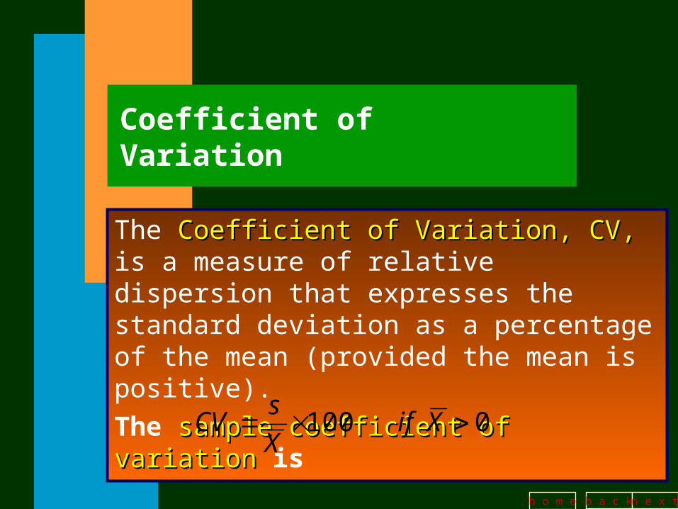
Coefficient of Variation

The Coefficient of Variation, CV,Coefficient of Variation, CV, is a measure of relative dispersion that expresses the standard deviation as a percentage of the mean (provided the mean is positive).

The sample coefficient of variationsample coefficient of variation is

0100 XifX

sCV


Coefficient of Variation

The population coefficient of variationpopulation coefficient of variation is

0100

ifCV


Percentiles and Quartiles

Data must first be in ascending order. PercentilesPercentiles separate large ordered data sets into 100ths. The PPth th percentilepercentile is a number such that P percent of all the observations are at or below that number.

QuartilesQuartiles are descriptive measures that separate large ordered data sets into four quarters.



The first quartile, Qfirst quartile, Q11, is another name for the

2525thth percentile percentile. The first quartile divides the ordered data such that 25% of the observations are at or below this value. Q1 is located in the .25(n+1)st position when the data is in ascending order. That is,

position ordered 4

)1(1

n

Q



The third quartile, Qthird quartile, Q33, is another name for the

7575thth percentile percentile. The first quartile divides the ordered data such that 75% of the observations are at or below this value. Q3 is located in the .75(n+1)st position when the data is in ascending order. That is,

position ordered 4

)1(33

nQ


Interquartile Range

The Interquartile Range (IQR)Interquartile Range (IQR) measures the spread in the middle 50% of the data; that is the difference between the observations at the 25th and the 75th percentiles:

13 QQIQR


Five-Number Summary

The Five-Number SummaryFive-Number Summary refers to the refers to the five descriptive measures: minimum, first five descriptive measures: minimum, first quartile, median, third quartile, and the quartile, median, third quartile, and the maximum.maximum.

imumimum XQMedianQX max31min


Box-and-Whisker Plots

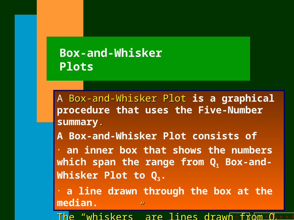
A Box-and-Whisker PlotBox-and-Whisker Plot is a graphical procedure that uses the Five-Number summary..

A Box-and-Whisker Plot consists of • an inner box that shows the numbers which span the range from Q1 Box-and-Whisker Plot to Q3.

• a line drawn through the box at the median.

The “whiskers” are lines drawn from QThe “whiskers” are lines drawn from Q11 to the to the

minimum vale, and from Qminimum vale, and from Q33 to the maximum value. to the maximum value.


Box-and-Whisker Plots (Excel)

Box-and-whisker Plot

16 10

15

20

25

30

35

40

45


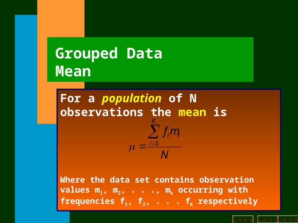
Grouped Data Mean

For a population of N observations the mean is

Where the data set contains observation values m1, m2, . . ., mk occurring with frequencies f1, f2, . . . fK respectively

N

mfK

iii

1


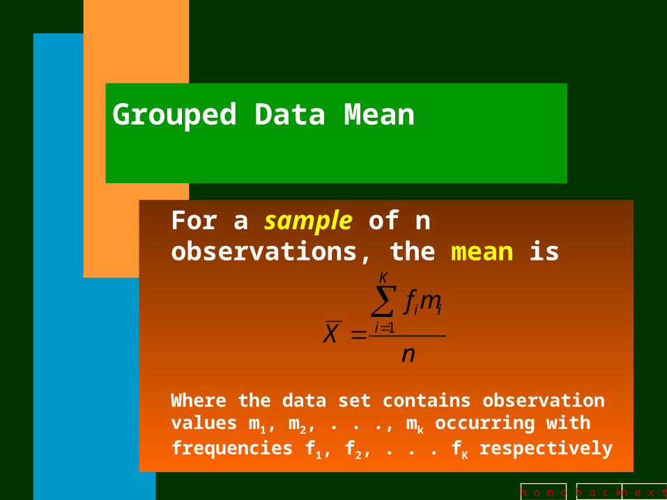
Grouped Data Mean

For a sample of n observations, the mean is

Where the data set contains observation values m1, m2, . . ., mk occurring with frequencies f1, f2, . . . fK respectively

n

mfX

K

iii

1


Grouped Data Variance

For a population of N observations the variance is

21

2

1

2

2

)(

N

mf

N

mfK

ii

K

iii i

Where the data set contains observation values m1, m2, . . ., mk occurring with frequencies f1, f2, . . . fK

respectively


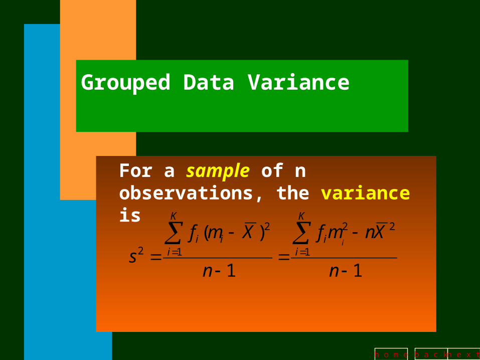
Grouped Data Variance

For a sample of n observations, the variance is

11

)(1

22

1

2

2

n

Xnmf

n

Xmfs

K

ii

K

iii i

classification of variables

Documents