classification: internal status: draft predicting characteristic loads for jackets and jack-ups...

Classification: Internal Status: Draft

Predicting characteristic loads for jackets and jack-ups

Shallow water location – quasi-static approachProblem definitionNeeded environmental informationDesign wave properties

Deeper water location – dynamic effects are importantProblem definitionNeeded environmental informationTime domain solution of equation of motion (steps of the analysis)Simple example of tie domain solution technique

Sverre HaverJanuary 2008

2

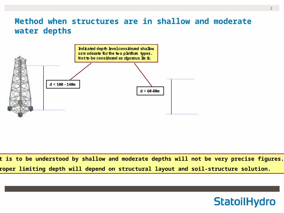
Method when structures are in shallow and moderate water depths

d < 100 - 140m

d < 60-80m

Indicated depth level considered shallowor moderate for the two platform types.Not to be considered as rigorous limit.

What is to be understood by shallow and moderate depths will not be very precise figures.

A proper limiting depth will depend on structural layout and soil-structure solution.

3

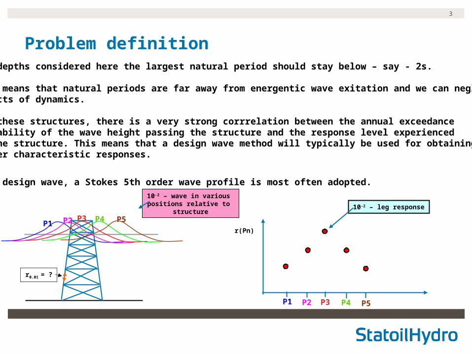
Problem definitionFor depths considered here the largest natural period should stay below – say - 2s.

This means that natural periods are far away from energentic wave exitation and we can neglect effects of dynamics.

For these structures, there is a very strong corrrelation between the annual exceedance probability of the wave height passing the structure and the response level experienced in the structure. This means that a design wave method will typically be used for obtainingproper characteristic responses.

As a design wave, a Stokes 5th order wave profile is most often adopted.

P1 P2 P4P3 P5

r0.01 = ?

r(Pn)

10-2 – wave in various positions relative to

structure

P1 P2 P3 P4 P5

10-2 – leg response

4

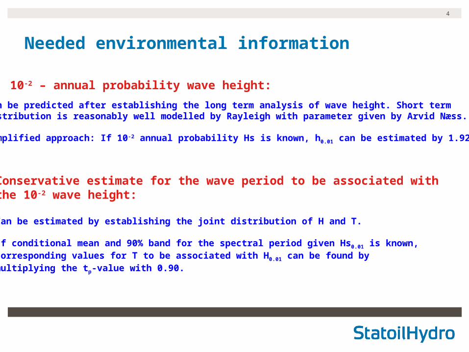
Needed environmental information

10-2 – annual probability wave height:

Conservative estimate for the wave period to be associated withthe 10-2 wave height:

Can be estimated by establishing the joint distribution of H and T.

If conditional mean and 90% band for the spectral period given Hs0.01 is known, corresponding values for T to be associated with H0.01 can be found by multiplying the tp-value with 0.90.

Can be predicted after establishing the long term analysis of wave height. Short term distribution is reasonably well modelled by Rayleigh with parameter given by Arvid Næss.

Simplified approach: If 10-2 annual probability Hs is known, h0.01 can be estimated by 1.92*hs0.01

5

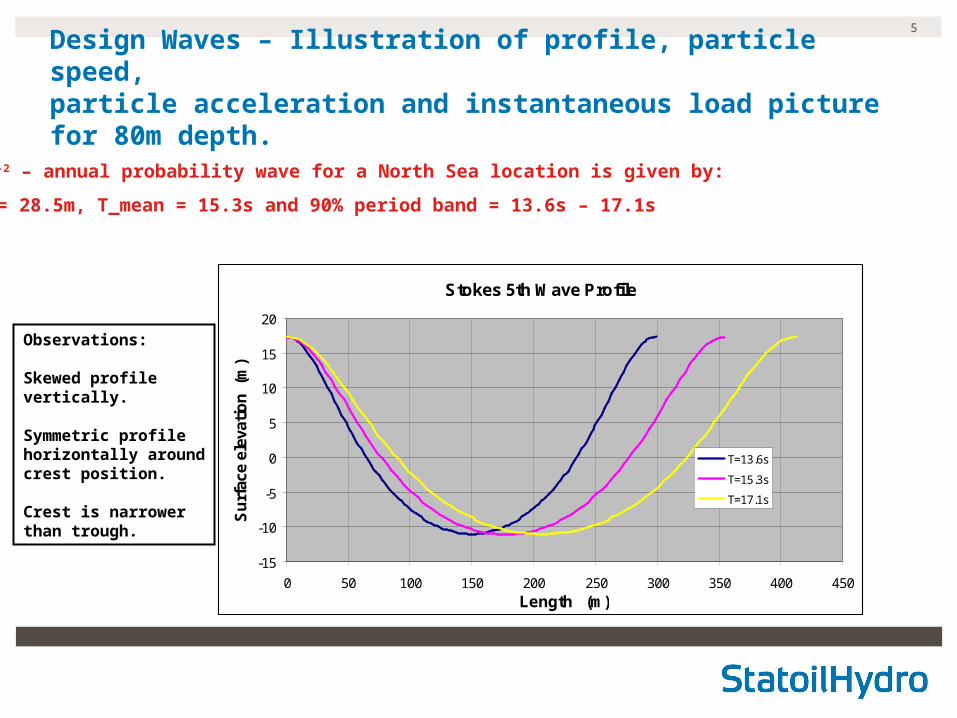
Design Waves – Illustration of profile, particle speed,particle acceleration and instantaneous load picture for 80m depth.

Stokes 5th Wave Profile

-15

-10

-5

0

5

10

15

20

0 50 100 150 200 250 300 350 400 450Length (m)

Su

rfac

e el

evat

ion

(m

)

T=13.6s

T=15.3s

T=17.1s

10-2 – annual probability wave for a North Sea location is given by:

H = 28.5m, T_mean = 15.3s and 90% period band = 13.6s – 17.1s

Observations:

Skewed profile vertically.

Symmetric profilehorizontally aroundcrest position.

Crest is narrower than trough.

6

Particle speed and accelerationDepth: 80m

Horisontal particle speed versus depth

Stoke 5th profile, H=28.5m

-80

-70

-60-50

-40

-30

-20

-100

10

20

0 2 4 6 8 10

Particle speed (m/s)

Dep

th le

vel (

m)

T=13.6s

T=15.3s

T=17.1s

Horizontal particle acceleration versus depth

-80

-70

-60

-50

-40

-30

-20

-10

0

0 0.5 1 1.5 2 2.5 3

Acceleration (m/s**2)

Dep

th le

vel

(m

)

T=13.6s

T=15.3s

T=17.1s

7

Instantaneous load picture

x

z

8

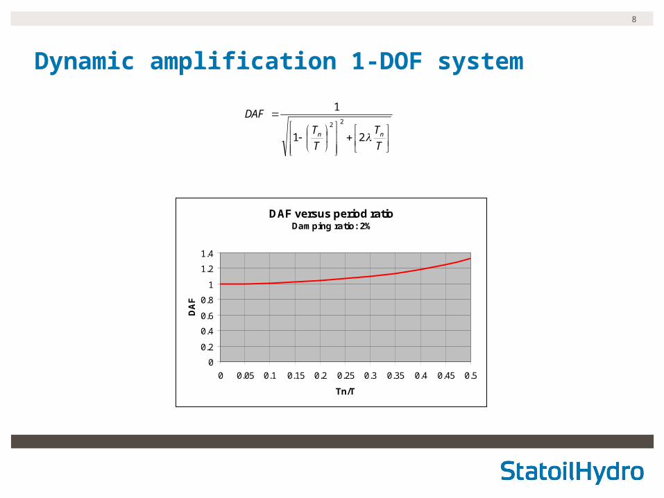
Dynamic amplification 1-DOF system

T

T

T

T

DAF

nn 21

122

DAF versus period ratio

Damping ratio: 2%

0

0.2

0.4

0.6

0.8

1

1.2

1.4

0 0.05 0.1 0.15 0.2 0.25 0.3 0.35 0.4 0.45 0.5

Tn/T

DA

F

9

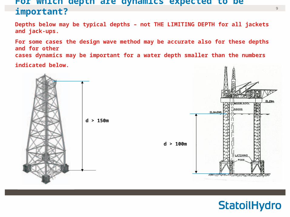
For which depth are dynamics expected to be important?Depths below may be typical depths – not THE LIMITING DEPTH for all jackets and jack-ups.

For some cases the design wave method may be accurate also for these depths and for other

cases dynamics may be important for a water depth smaller than the numbers indicated below.

d > 150m

d > 100m

10

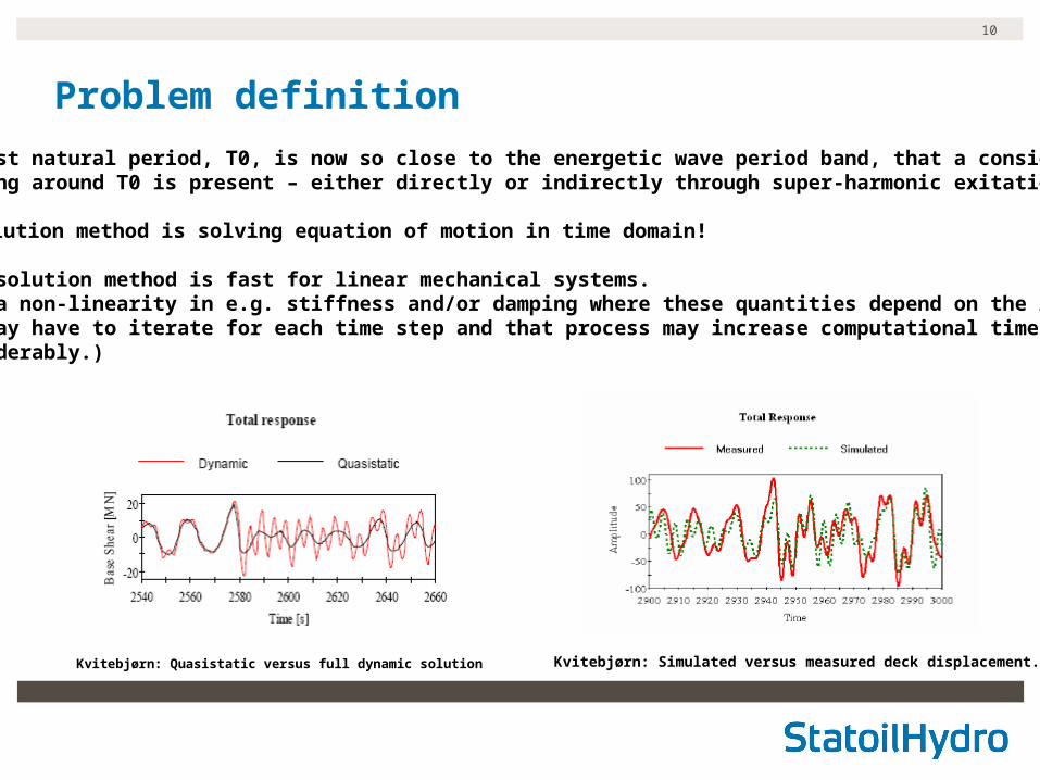
Problem definition

Largest natural period, T0, is now so close to the energetic wave period band, that a considerable loading around T0 is present – either directly or indirectly through super-harmonic exitation.

Solution method is solving equation of motion in time domain!

This solution method is fast for linear mechanical systems. (For a non-linearity in e.g. stiffness and/or damping where these quantities depend on the responseone may have to iterate for each time step and that process may increase computational time considerably.)

Kvitebjørn: Quasistatic versus full dynamic solution Kvitebjørn: Simulated versus measured deck displacement.

11

Time domain analysis

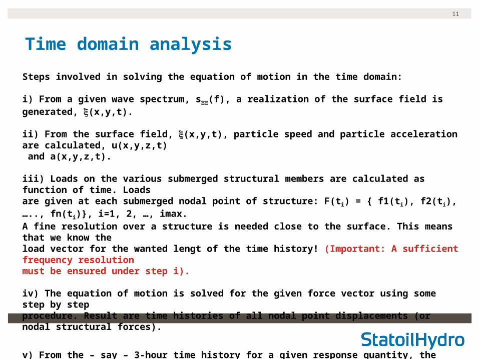
Steps involved in solving the equation of motion in the time domain:

i) From a given wave spectrum, s(f), a realization of the surface field is generated, (x,y,t).

ii) From the surface field, (x,y,t), particle speed and particle acceleration are calculated, u(x,y,z,t) and a(x,y,z,t).

iii) Loads on the various submerged structural members are calculated as function of time. Loadsare given at each submerged nodal point of structure: F(ti) = { f1(ti), f2(ti), ….., fn(ti)}, i=1, 2, …, imax.A fine resolution over a structure is needed close to the surface. This means that we know the load vector for the wanted lengt of the time history! (Important: A sufficient frequency resolutionmust be ensured under step i).

iv) The equation of motion is solved for the given force vector using some step by step procedure. Result are time histories of all nodal point displacements (or nodal structural forces).

v) From the – say – 3-hour time history for a given response quantity, the distribution function for response maxima and for the 3-hour extreme value can be estimated. This is short term analysisof the response for a non-linear response problem.

12

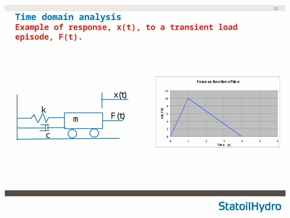
Time domain analysis Example of response, x(t), to a transient load episode, F(t).

m

c

kF(t)

x(t)

Force as function of time

0

2

4

6

8

10

12

0 1 2 3 4 5 6Time (s)

x(t)

, F

(t)

13

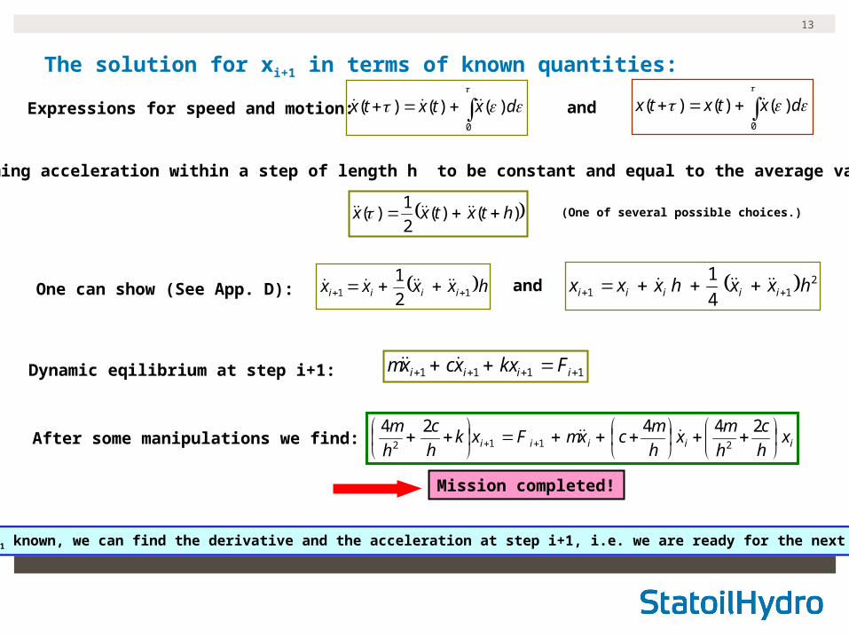
The solution for xi+1 in terms of known quantities:

0

)()()( dxtxtx

0

)()()( dxtxtx

)()(2

1)( htxtxx

hxxxx iiii 11 2

1

211 4

1hxxhxxx iiiii

1111 iiii Fkxxcxm

iiiii x

h

c

h

mx

h

mcxmFxk

h

c

h

m

244242112

Expressions for speed and motion: and

Assuming acceleration within a step of length h to be constant and equal to the average value:

(One of several possible choices.)

One can show (See App. D): and

Dynamic eqilibrium at step i+1:

After some manipulations we find:

Mission completed!

With xi+1 known, we can find the derivative and the acceleration at step i+1, i.e. we are ready for the next step!

14

Numerical exampleInitial conditions: 000 xx

m

FxFkxxcxm 0

00000 , here = 0.

m = 0.2279 c = 0.0955 k = 1

System characteristics: T0 = 3s, lambda = 0.10

Time domain solution of motion

-20

-15

-10

-5

0

5

10

15

20

0 2 4 6 8 10Time (s)

x(t)

, F

(t)

Response

Force function

15

Response for reduced duration of load relative the natural period

Time domain solution of motionlambda = 0.1, T/T0 =1

-20

-15

-10

-5

0

5

10

15

0 2 4 6 8 10Time (s)

x(t)

, F

(t)

Response

Force function

Time domain solution of motionlambda = 0.1, T/T0 =0.4

-20

-15

-10

-5

0

5

10

15

0 2 4 6 8 10Time (s)

x(t)

, F

(t)

Response

Force function


-20

-15

-10

-5

0

5

10

15

0 2 4 6 8 10Time (s)

x(t)

, F

(t)

Response

Force function


-20

-15

-10

-5

0

5

10

15

0 2 4 6 8 10Time (s)

x(t)

, F

(t)

Response

Force function

16

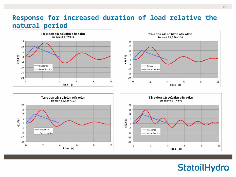
Response for increased duration of load relative the natural period


-20

-15

-10

-5

0

5

10

15

0 2 4 6 8 10Time (s)

x(t)

, F

(t)

Response

Force function


-20

-15

-10

-5

0

5

10

15

20

0 2 4 6 8 10Time (s)

x(t)

, F

(t)

Response

Force function


-20

-15

-10

-5

0

5

10

15

20

0 2 4 6 8 10Time (s)

x(t)

, F

(t)

Response

Force function


-20

-15

-10

-5

0

5

10

15

20

0 2 4 6 8 10Time (s)

x(t)

, F

(t)

Response

Force function

17

Effect of dampingTime domain solution of motion

lambda = 1, T/T0 =2

-20

-15

-10

-5

0

5

10

15

0 2 4 6 8 10Time (s)

x(t)

, F

(t)

Response

Force function


-20

-15

-10

-5

0

5

10

15

0 2 4 6 8 10Time (s)

x(t)

, F

(t)

Response

Force function


-20

-15

-10

-5

0

5

10

15

20

0 2 4 6 8 10Time (s)

x(t)

, F

(t)

Response

Force function


-20

-15

-10

-5

0

5

10

15

20

0 2 4 6 8 10Time (s)

x(t)

, F

(t)

Response

Force function