classification for predicting offender affiliation with murder victims

Expert Systems with Applications 38 (2011) 13518–13526

Contents lists available at ScienceDirect

Expert Systems with Applications

journal homepage: www.elsevier .com/locate /eswa

Classification for predicting offender affiliation with murder victims

Rui Yang, Sigurdur Olafsson ⇑Department of Industrial and Manufacturing Systems Engineering, Iowa State University, 3004 Black Engineering, Ames, IA 50011, USA

a r t i c l e i n f o

Keywords:Homicide dataClassificationDecision treeSupport vector machineRandom forest

0957-4174/$ - see front matter � 2011 Elsevier Ltd. Adoi:10.1016/j.eswa.2011.03.051

⇑ Corresponding author. Tel.: +1 515 294 8908; faxE-mail address: [email protected] (S. Olafsson)

a b s t r a c t

The National Incident-Based Reporting System (NIBRS) is used by law enforcement to record a detailedpicture of crime incidents, including data on offenses, victims and suspected arrestees. Such incident datalends itself to the use of data mining to uncover hidden patterns that can provide meaningful insights tolaw enforcement and policy makers. In this paper we analyze all homicide data recorded over one year inthe NIBRS database, and use classification to predict the relationships between murder victims and theoffenders. We evaluate different ways for formulating classification problems for this prediction andcompare four classification methods: decision tree, random forest, support vector machine and neuralnetwork. Our results show that by setting up binary classification problems to discriminate each typeof victim–offender relationship versus all others good classification accuracy can be obtained, especiallyby the support vector machine method and the random forest approach. Furthermore, our results showthat interesting structural insight can be obtain by performing attribute selection and by using transpar-ent decision tree models.

� 2011 Elsevier Ltd. All rights reserved.

1. Introduction

Homicide is a very infrequent crime. In 1999, for example, therewere 15,530 homicides reported (Federal Bureau of Investigation,1984–2000) among an estimated population of 272.9 million inthe United States (US Bureau of the Census, 1983). Despite its rar-ity, as homicide is a particularly serious crime and is highly visibleto the public (Ermann & Lundman, 2002), any patterns that revealinsights into homicide offenders would be useful for both lawenforcement and policy makers. Patterns involving the victim–of-fender relationship are of particular interest because homicidesare closely linked with the social activities of individuals, whichis to a large extent shaped by the victim–offender relationship(Flewelling & Williams, 1999). Such patterns could potentially bediscovered using data mining methods based on the surveillancedata available through the National Incident-Based ReportingSystem (NIBRS) database. In this paper we propose and evaluatethe use of classification to predict the relationships betweenhomicide victims and offenders based on various independentvariables available in the NIBRS database.

Data mining is a semi-automated process of extracting mean-ingful, previously unknown patterns from large databases (Han &Kamber, 2001; Olafsson, Li, & Wu, 2008). The increased popularityof data mining is partially due to data collection and storage beingeasier, leading to massive databases such as the NIBRS database.While such databases contain a wealth of valuable data, meaning-

ll rights reserved.

: +1 515 294 3505..

ful patterns are often hidden and unexpected, which implies thatthey may not be uncovered by hypothesis-driven methods. Induc-tive data mining methods, which learn directly from the data with-out an a priori hypothesis, can then be used to uncover the hiddenpatterns. The data mining process consists of numerous steps,including data integration and preprocessing and induction of amodel with a learning algorithm. All data mining starts with aset of data called the training set, which consists of instancesdescribing the observed values of certain attributes. These in-stances are then used to learn a pattern. One of the main ap-proaches to learning is classification. In classification the trainingdata is labeled, meaning that each instance is identified as belong-ing to one of two or more pre-defined classes, and an inductivelearning algorithm is used to create a model that discriminates be-tween those class values. This model can then be used to classifyany new instances.

In recent years data mining techniques have been found to beuseful in many application areas related to crime analysis andlaw enforcement (e.g., Keppers & Schafer, 2006; Poelmans, Elzinga,Viaene, Van Hulle, & Dedene, 2009). As an example, data mining ofhistorical incident data can be used to induce a model that predictsthe threat level for different areas and time periods, followingwhich force deployment and other preventive measures can be ta-ken to address the threats. For this purpose, Abu Hana, Freitas, andOliveira (2008) extracted a set of features from crime scene to clas-sify the violent crime as attacking from inside or outside of thescene. Crime hot-spot location has also been predicted using datamining methods in order to improve public safety (Grubesic,2006; Kianrnehr & Alhajj, 2008). However, despite several success-

http://dx.doi.org/10.1016/j.eswa.2011.03.051

mailto:[email protected]

http://dx.doi.org/10.1016/j.eswa.2011.03.051

http://www.sciencedirect.com/science/journal/09574174

http://www.elsevier.com/locate/eswa

R. Yang, S. Olafsson / Expert Systems with Applications 38 (2011) 13518–13526 13519

ful studies and an abundance of incident data available throughNIBIRS and related sources, the use of data mining in law enforce-ment is still relatively new (Akiyama & Nolan, 1999; Noonan &Vavra, 2007).

Homicides have long recognized as heterogeneous crimes andthe various homicide subtypes often have their own predictorsand causes (Wolfgang, 1958). Researchers thus often study homi-cide events based on conceptually meaningful subtypes of homi-cide. A majority of these studies focus on the victim–offenderrelationship. One reason is that homicide is tightly coupled withthe social activities of individuals while victim–offender relation-ships shaped in this social process reveal some particular structuralconditions (Flewelling & Williams, 1999; Williams & Flewelling,1988). Decker (1996) demonstrated the important consequencesof victim–offender relationships as offering some protections andincreasing the likelihood that fatal interactions will occur amongothers. Last and Fritzon (2005) showed that this relationship sig-nificantly influences the type of aggression displayed in a homi-cide. Not only do the classification based on victim–offenderrelationship work well with the theoretical prediction of homicidealong instrumental and expressive lines, but also consists with tra-ditional theories such as disorganization theory and deprivationtheory. Williams and Flewelling (1988) provided evidence of theimportance of social disorganization factors to studies of victim–offender relationships in homicide. Deprivation theory explainsthe different effects on victim–offender relationships in homicideunder blocked economic opportunities (Braithwaite, 1979; Parker,2001; Williams & Flewelling, 1988). The importance of the victim–offender relationship is therefore well established, but the use ofdata mining methods to automatically discover patterns of homi-cide victim–offender relationships has to the best of our knowl-edge not been considered before.

The remainder of the paper is organized as follows. In Section 2we describe the NIBIRS database that provides the data source forthis study. In Section 3 we discuss the type of classification prob-lems and methods to be considered for this database. Sections 4–6 describe our results for three different formulations of the classi-fication task, and finally Section 7 contains some concludingremarks.

Fig. 1. National coverage of the murder cases in NIBRS in 2005.

Table 1Types and frequencies of victim-offender relationships.

Proportion Count

Family 0.16 (431)Close to Family 0.07 (199)Acquaintance 0.28 (792)Stranger 0.10 (267)Unknown 0.39 (1091)

2. The NIBRS database

After the Federal Bureau of Investigation (FBI) significantly im-proved the existing Uniform Crime Reporting (UCR) summaryreporting system by creating what is known as the National Inci-dent-Based Reporting System (NIBRS), the infrastructure is nowavailable for crime analysis using data mining. Law enforcemententers data on known incidents into the NIBRS database, includingdata on offenses, victims, suspected arrestees, and other incidentrelated information. As opposed to the UCR, which reflects aggre-gate information, the NIBRS captures detailed picture of each inci-dent, which is precisely the level of data needed for successful datamining. Many researchers have taken advantage of different as-pects of the detail provided in the NIBRS database (see e.g., Chilton& Jarvis, 1999; Faggiani & McLaughlin, 1999; Stolzenberg &D’alessio, 2000).

The data for this study was obtained from the 2005 records inthe NIBRS database. In that year a total of 3207 completed homi-cide incidents were reported as murder/non-negligent manslaugh-ter (corresponding to code ‘‘09A’’ in NIBRS), but the availableinformation for each incident is in some cases incomplete. Herewe focus on the victim–offender relationship, so for the purposeof this study we are interested in personal victims; and 3587 suchvictims were extracted from the NIBRS as being connected to those3207 incidents. Among these there are 396 victims whose offend-

ers have not been found, and another 411 victims still alive, whomost suffer from assault, robbery, and burglary. There are therefore2780 deceased victims, which provide the basis for the analysis.Although not all states are represented in the data set the data iscomprised of states from a variety of geographic regions and pop-ulation sizes, and thus provides good national coverage (see Fig. 1).

Homicide relationship types are coded into four categories orclasses: homicide committed by family members, homicide com-mitted by someone very close to the family (e.g., a babysitter, boy-friend or girlfriend, or ex-spouse), homicide committed byacquaintances (e.g., friend, neighbor, employee or employer), andhomicide committed by strangers. When there are several victimsas well as several offenders involved we generate a profile for eachvictim. If many offenders were involved, we consider the offenderwith the closest relationship to the victim(s) to be the primary of-fender. The victims and offenders link the incident and associatedoffenses by originating agency identifier (ORI), incident number,victim sequence number and offender sequence number. The mur-der case may involve multiple offenses. In order to shed some lighton the context of homicide, the corresponding offenses are addedinto the murder record, and a binary variable is introduced to indi-cate whether or not the location changes in an incident.

To gain some insights into the characteristics of the homicidesthat are being studied, we consider a few relevant summary statis-tics. As can be seen from the Table 1, of the homicides where thevictim–offender relationship is known most homicides are perpe-trated by acquaintances (28%), followed by murders committedby family members (16%). Most incidents involve a single offense(79.8%), one victim (84.1%) and one offender (71.2%). The victimsrange from newborn babies to a senior citizen at ninety-four yearsold, with the average age of victims is 32.7 years. Three-fourths ofvictims are male, and other one-fourth is female. Murders are morelikely to occur in the hours of 11pm to 2am, but least likely to occurin the hours of 5am to 7am. Murders are more likely than averageto occur on a Saturday or a Sunday while least likely on a Wednes-day. Out of 2907 homicides, 587 cases involve multiple offenses,which are most likely to be assault, weapons violation and robbery.The hotspots where homicides occur most frequently are resi-dence, highway/road and parking lots. The remaining specified

13520 R. Yang, S. Olafsson / Expert Systems with Applications 38 (2011) 13518–13526

locations count for only 12% of total number of incidents. There is asingle type of weapon used in 2606 cases out of 2907 incidents(89.6%), two types of weapons in 66 cases (2.3%), and more thantwo kinds of weapons in six cases (0.2%). The most common weap-ons are handguns (32.7%), guns (21.4%), then knives (12.1%), andhuman objects such as feet and hand (7.6%).

3. Classification of homicide data

Our objective is to classify the type of homicide according to thefour types of victim–offender relationship based on the indepen-dent variables available in the NIBRS database. To that end, wecompare the performance of four types of classification algorithms:decision trees, random forest, neural networks, and support vectormachines (SVM). We now briefly discuss each of those methods.

Although decision trees do not usually provide the best predic-tion accuracy for classifications, they are simple and interpretable,and can be used to gain insights into the interaction between attri-butes (Breiman, Friedman, Olshen, & Stone, 1984; Quinlan, 1993).The usual process of decision tree induction is to construct a treein a top-down manner by selecting variables one at a time andsplitting the data according to some splitting criterion (Mingers,1989), such as information gain ratio or the Gini index. Here ourprimary interest in decision trees is the insights that can be ob-tained from the decision trees by analyzing specific scenarios rep-resented in the trees. Such insights can then be used to furtherenhance the decisions regarding intervention techniques and mod-els that can reduce the occurrence of such homicides.

Random forest is an ensemble classifier (Dietterich, 2000),which uses bagging to make a prediction based on the vote of mul-tiple decision trees (Breiman, 2001). As might be expected, thisusually significantly improves the accuracy of the classificationbut at the same time the interpretability of the decision trees isat least partially lost. Bagging helps tree classifier gain accuracyby reducing the variance in the error estimates; although the meanis the same the standard deviation of the errors from averaging re-sults of multiple trees is decreased. Error rate, votes, variableimportance and proximity would be provided by the informationfor each tree, and in particular the out-of-bag (OOB) cases for eachtree. There are two ways to measure variable importance usingrandom forests. The first one is to consider individual variableimportance. The approach is to randomly permute the values ona variable in the OOB cases and predict the class for these cases,and then subtract the number of votes for the correct class in thevariable-permuted OOB data from the number of votes for the cor-rect class in the real OOB data. The average of this number over alltrees in the forest is the raw importance score for that variable. Ifthe value is small, then the variable is not very important. The sec-ond approach is to consider importance of a set of combined vari-ables. Every time a split of a node is made on a variable, theimpurity for the two descendent nodes is smaller than that ofthe parent node. Adding up the decreases for each individual var-iable over all trees in the forest gives a variable importance thatis usually consistent with the permutation importance measure.Both the accuracy at the split and Gini measure of impurity areused to evaluate variable importance. These extensive sampletechniques make it unnecessary to break the data into trainingand testing set.

Support vector machines (SVM) trace their origins to the semi-nal work of Vapnik and Lerner (1963) and Mangasarian (1965). TheSVM approach to classification is to identify a hyperplane that bestseparates instances that take different class values (Vapnik, 1998).One of the strengths of SVM is that the original data can be mappedinto to a higher dimensional space via what is called a kernel func-tion, identify the hyperplane in this higher dimension and then

map it back to the original space. This enables SVM to constructnonlinear classifiers that linearly separate the data points in thehigher dimensional space. Popular kernel functions include linear,polynomial, Gaussian, and tangent hyperbolic kernels. In this workpolynomial kernels were used.

Neural networks are one of the classic machine learning meth-ods that can be used for classification (Ripley, 1996), and in thiswork we use a feed-forward neural network learning algorithmas the final classification algorithm considered. This model has asingle hidden layer with five neurons and univariate output values.The inputs to the network correspond to the attributes measuredfor each training instance. These inputs pass through the inputlayer and are then weighted and fed simultaneously to a hiddenlayer of units. The weighted outputs of the hidden layer approacha threshold, at which it emits the network’s prediction for given in-stances. In addition to their high tolerance of noisy data, one of theadvantages of neural networks is to classify patterns when youmay have little knowledge of the relationships between attributesand classes.

An alternative to the four class-value problem (that is, wherethe class values are ‘‘Family,’’ ‘‘Close-to-Family,’’ ‘‘Acquaintance,’’and ‘‘Stranger’’) is to set up binary classification problems wherethe goal is to discriminate between one specific victim–offenderrelationship and all others (e.g., ‘‘Family’’ versus ‘‘non-Family’’).This results in four binary classification problems, one for eachclass value. A binary class is sometimes easier to predict, but thisalso raises an issue of class imbalance (Japkowicz, 2000). For exam-ple, there are 199 instances of the class value ‘‘Close-to-Family’’and 1490 instances of all others. Thus, a binary classification modelpredicting ‘‘Close-to-Family’’ versus others could completelyignore the minority class (‘‘Close-to-Family’’) and be approxi-mately 88% accurate. However, it would also be complete useless.An effective method for addressing class imbalance is resamplingthe database, that is, either undersampling the majority class valueor oversampling the minority class value(s). In this study we firstdivide the dataset into training (70%) and test (30%) data, and thensample the training set with replacement according to a biasedsampling distribution. The sampling distribution oversamples theminority class and undersamples the majority class so that the ex-pected proportion of each of the two class values is the same in thesampled training set. The unbiased test set is then used to evaluatethe accuracy of the prediction.

4. Discriminating between all victim–offender relationshiptypes

The first part of this study was an effort to induce classificationmodels to distinguish between all four victim–offender relation-ships, namely ‘‘Family’’, ‘‘Close-to-Family’’, ‘‘Acquaintance’’, and‘‘Stranger’’ (see Table 1). The estimated classification accuracy foreach of the four classification methods was found to be unaccept-ably large. For example, for the random forest classifier, which con-structs 2000 trees and optimizes the number of variables at eachsplit, what is referred to as the out-of-bag (OOB) estimate of errorrate is 38.2% overall. To provide some insights into why this error isso large, consider the confusion matrix of the random forest classi-fier (Table 2). From this table we can observe that the majorityclass of ‘‘Acquaintance’’ is predicted too many times. Specifically,when the true relationship is ‘‘Close-to-Family’’ or ‘‘Stranger’’ therelationship is incorrectly predicted as ‘‘Acquaintance’’. Similarly,the second most common class, namely ‘‘Family’’, is often pre-dicted when other relationships are correct, especially when thetrue relationship is ‘‘Close-to-Family’’. Predicting the majority classvalue of ‘‘Acquaintance’’ has much lower error than the other classvalues.

Table 2This table shows the confusion matrix and the error rates of the random forest. Eachcolumn shows instances predicted to have the same class value, and each row showsthe true class value of those instances.

Predicted class

Family Close-to-Family

Acquain-tance

Stranger Error

True class Family 197 20 121 3 42.2%Close-to-Family 61 36 70 1 78.6%Acquaintance 54 15 579 8 11.7%Stranger 13 3 161 45 79.7%

Table 3Most predictive attributes for each offender-victim relationship category.

Family Close-to-Family Acquaintance Stranger

Victim’s age Victim’s sex Victim’s sex LocationLocation Lovers Victim’s age Total victimsVictims sex Number of offenders State StateNumber of

offendersVictim’s age Victim’s race Hour

State State Hour Number of offenders

Table 4Results of four classifiers to distinguish relationship between Family and non-Family.

Model Training data Test data

Totalerror

TP rate(non-Family)

FP rate(Family)

Totalerror

TP rate(non-Family)

FP rate(Family)

Random forest 11.7% 20.3% 3.1% 8.9% 10.0% 5.3%Tree 22.7% 27.0% 18.4% 31.8% 34.7% 22.8%Neural network 0 0 0 5.6% 5.7% 5.3%SVM 0 0 0 4.1% 3.4% 6.1%

Table 5Results of four classifiers to distinguish relationship between Close-to-Family andnon-Close-to-Family.


Totalerror

TP rate(non-CloseF)

FP rate(CloseF)

Totalerror

TP rate(non-CloseF)

FP rate(CloseF)

Random forest 6.3% 12.0% 0.7% 6.5% 7.4% 0Tree 15.9% 24.9% 6.9% 23.6% 25.9% 7.1%Neural network 0 0 0 4.1% 4.2% 3.6%SVM 0 0 0 2.6% 2.5% 3.6%

Table 6Results of four classifiers to distinguish relationship between Acquaintance and non-Acquaintance.


Totalerror

TP rate(non-Acqu)

FPrate(Acqu)

Totalerror

TP rate(non-Acqu)

FP rate(Acqu)

Random forest 28.6% 44.9% 12.3% 6.1% 8.2% 3.7%Tree 28.6% 37.5% 16.5% 27.0% 29.9% 23.7%Neural network 7.4% 7.0% 7.8% 10.8% 11.5% 10.1%SVM 0 0 0 6.3% 7.0% 5.5%

Table 7Results of four classifiers to distinguish relationship between Stranger and non-Stranger.



Even though it appears difficult to achieve high classificationaccuracy for discriminating between all four class values otherstructural information may be of interest. For example, it may beof value to know which attributes are the most important for dis-criminating the four types of victim–offender relationships, as wellas which attributes are most important for predicting each individ-ual type of relationship. As described in Section 3, this can beachieved using the random forest results. For example, the randomforest outputs the top eight predictors as: hour, victim’s age, loca-tion, number of offenders, state, number of victims, and victim’srace. The five most predictive attributes for each class value, listedin order of importance, are shown in Table 3. It is interesting tonote both the overlap and differences between those attributes.For example, both the victim’s age and sex are important predic-tors when there is any relationship between victim and offender,but not when they are strangers. The most predictive attributesfor a stranger classification are external to the offender and victim(that is, location, state and hour of the day when the crime occurs)and the number of people involved (both victims and offenders).

Totalerror

TP rate(non-Stranger)

FP rate(Stranger)

Totalerror

TP rate(non-Stranger)

FP rate(Stranger)

Random Forest 7.3% 13.3% 1.2% 5.0% 5.7% 1.4%Tree 20.0% 25.1% 14.9% 25.7% 28.0% 13.5%Neural Network 0 0 0 5.4% 6.2% 1.4%SVM 0 0 0 3.0% 3.1% 2.7%

5. Predicting each victim–offender relationship type

As noted in Section 3 above, an alternative to predicting all fourclass values is to set up binary classification problems where thegoal is to discriminate between one specific victim–offender rela-tionship and all others. As binary class is sometimes easier to pre-dict we set up four such problems, one for each type of relationshipand use resampling to address the class imbalance issue as de-scribed in Section 3. The results for all four classifiers are reportedin Tables 4–7 , which show both the estimated training error andthe unbiased estimate based on the test data. In addition to the to-tal error, the tables also report both the false-positive (FP) rate forthe target class value (e.g., ‘‘Family’’) and the true-positive (TP) ratefor the other class value (e.g., ‘‘non-Family’’).

From Table 4 we note that it is in fact possible to predict thebinary class values of victim–offender relationship being ‘‘Family’’versus ‘‘non-Family’’ with much higher accuracy than the four-class-value problem. For example, with support vector machinesa model is constructed that has an estimated error rate of only4.1%, and the random forest model has an estimated error of 8.9%versus 38.2% for the four-class-value problem.

Similar observations are indicated for discriminating ‘‘Close-to-Family’’ versus ‘‘not-Close-to-Family’’ by the results reported

in Table 5. The SVM model is again most accurate with an esti-mated accuracy of 2.6%; and the same is true for discriminating‘‘Stranger’’ versus ‘‘non-Stranger,’’ where the estimated SVM errorrate is 3.0% (see Table 7). For discriminating ‘‘Acquaintance’’ versus‘‘non-Acquaintance’’ the random forest model is slightly betterthan the SVM at 6.1% error rate (see Table 6), although thedifference between the two models is not significant.

The SVM model provides the lowest estimated error rate forthree out of the four classification problems, the random foresthas the lowest estimated error for one, and neural networks arethe second lowest for three out of four problems. Overall we ob-serve that those three methods all perform fairly well for this clas-sification task with respect to prediction accuracy, although theseresults indicate that support vector machines tend to be betterthan the other two.

Age

Location

Age

Others, Commercial, Highway, Public,Parking, Woods, Jail, Church Residence, Hospital

SexRace

# OffenderStateMonth

Non-Family Hour Hour Hour Hour

Argument?

Family

Non-Family Non-Family

Non-Family

Non-FamilyNon-Family

Non-Family

Non-Family

Family

FamilyFamilyFamily

Family

[10, 70) [0, 10) |[70, ∞) [15, 40) [0, 15) |[40, ∞)

Black, Asian White, Native F M

Jan, Feb, Mar, Apr, Sep, Oct, Dec May, Jun,

Jul, Aug, Nov CO,CT,KS,MI,ND,OH,SC,TN,TX,UT,VA,WV

ID,KY,LA,MA,MT,NH,RI,VT,WI

=1 ≥2

2, 6,10,11,12,15,17, 20-22

23,0,1,3,4,5,7,9,13,14,16,18,19,

No Yes

1,2,6,8,9,203,4,7,10-19,

21-0 5-22, 1, 223,0,3,4, 1,2,5,9,10-12,

18-20,22,23 0,3,4,8,13,1

4,17,21

Total: 416 F:63 NF:353

Total: 26 F:19 NF:7

Total: 308 F:265 NF:43

Total: 33 F:1 NF: 32

Total: 85F:7 NF:78

Total: 16 F:3 NF:13

Total: 223 F:155 NF:68

Total: 42 F:11 NF:31


Total: 13 F:1 NF:12

Total: 49 F:8 NF:41


Total: 228 F:175 NF:53

Total: 29 F:2 NF:27

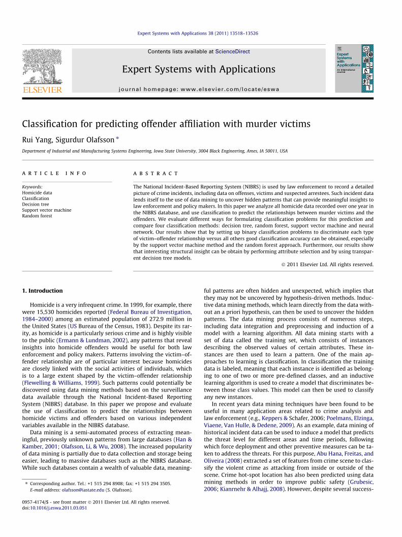
Fig. 2. Decision tree to discriminate homicide between family members.

Lovers’ quarrel?

Sex

Age

M F

StateHour

MonthNon-CloseF

Hour

State Hour

CloseF

Non-CloseF

Non-CloseF CloseF

CloseF

Non-CloseF Non-CloseFCloseF CloseF

No Yes <15 or ≥60 [15, 60)

0-4,7,8,13-23 6, 9,10,12 1,3,4,6-10,12,14-19,22,23 5,11,13,20,21,0

CO,KY,NH,RI,WI,WV

AR,CT,IA,ID,KS,LA,MA,MI,MT,ND,OH,OR,SC,TN,TX,UT,VA

Jan, Feb, May, Jun,Aug, Oct, Nov

Mar, Apr, Sep, Dec

AR,CO,CT,ID,KS,OH,SC,TX,VA

IA,MI,OR,TN

2-5,7,8,12,14,15,19-23 0,1,9-11,17

Total: 41 C:8 NC:33

Total: 73 C:63 NC:10

Total: 69 C:0 NC:69

Total: 697 C:116 NC:581

Total: 695 C:580 NC:115

Total: 24 C:20 NC:4

Total: 24 C:0 NC:24

Total: 33C:30 NC:3

Total: 14 C:0 NC:14

Total: 54 C:45 NC:9

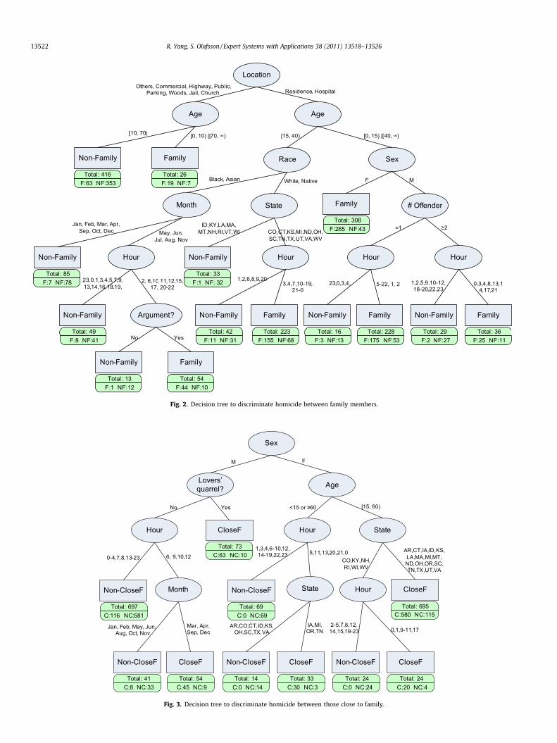
Fig. 3. Decision tree to discriminate homicide between those close to family.


# Offender

Non-Acquaintance

Sex

Age

F M

Acquaintance

Month Age

Non-Acquaintance

Non-Acquaintance

Acquaintance

AcquaintanceAcquaintance

=1 ≥2

State

Jan Apr May Jun Jul Aug Sep Dec Feb Mar Oct [25, 70) [15, 25)

<15 or ≥70 [15, 70)

Race

AR,CT,IA,ID,KS,KY,LA,MI,ND,OH,OR,RI,SC,TN,TX,UT,VA,WV CO,MA,MT,NH,SD,VT,WI

Weekday

AcquaintanceNon-Acquaintance

White, Native, Asian

Tue, Thu, Sun

Black

Mon, Wed, Fri, Sat

Total: 90 A:31 NA:59

Total: 50 A:41 NA:9


Total: 298 A:56 NA:242


Total: 117 A:68 NA:49

Total: 283 A:212 NA:71

Total: 31 A:23 NA:8

Total: 219 A:139 NA:80

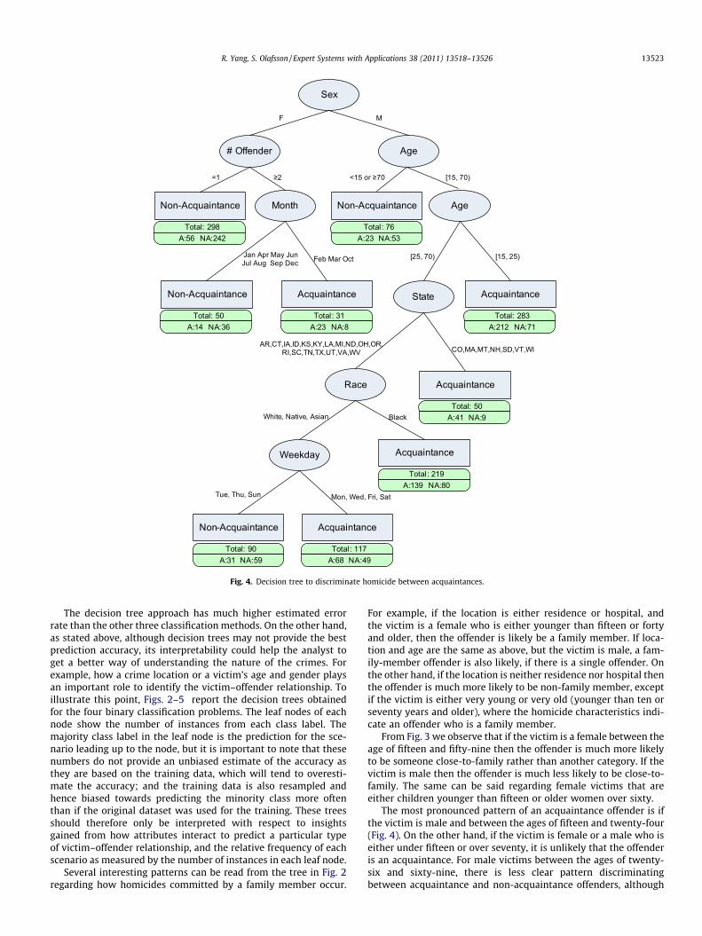
Fig. 4. Decision tree to discriminate homicide between acquaintances.


The decision tree approach has much higher estimated errorrate than the other three classification methods. On the other hand,as stated above, although decision trees may not provide the bestprediction accuracy, its interpretability could help the analyst toget a better way of understanding the nature of the crimes. Forexample, how a crime location or a victim’s age and gender playsan important role to identify the victim–offender relationship. Toillustrate this point, Figs. 2–5 report the decision trees obtainedfor the four binary classification problems. The leaf nodes of eachnode show the number of instances from each class label. Themajority class label in the leaf node is the prediction for the sce-nario leading up to the node, but it is important to note that thesenumbers do not provide an unbiased estimate of the accuracy asthey are based on the training data, which will tend to overesti-mate the accuracy; and the training data is also resampled andhence biased towards predicting the minority class more oftenthan if the original dataset was used for the training. These treesshould therefore only be interpreted with respect to insightsgained from how attributes interact to predict a particular typeof victim–offender relationship, and the relative frequency of eachscenario as measured by the number of instances in each leaf node.

Several interesting patterns can be read from the tree in Fig. 2regarding how homicides committed by a family member occur.

For example, if the location is either residence or hospital, andthe victim is a female who is either younger than fifteen or fortyand older, then the offender is likely be a family member. If loca-tion and age are the same as above, but the victim is male, a fam-ily-member offender is also likely, if there is a single offender. Onthe other hand, if the location is neither residence nor hospital thenthe offender is much more likely to be non-family member, exceptif the victim is either very young or very old (younger than ten orseventy years and older), where the homicide characteristics indi-cate an offender who is a family member.

From Fig. 3 we observe that if the victim is a female between theage of fifteen and fifty-nine then the offender is much more likelyto be someone close-to-family rather than another category. If thevictim is male then the offender is much less likely to be close-to-family. The same can be said regarding female victims that areeither children younger than fifteen or older women over sixty.

The most pronounced pattern of an acquaintance offender is ifthe victim is male and between the ages of fifteen and twenty-four(Fig. 4). On the other hand, if the victim is female or a male who iseither under fifteen or over seventy, it is unlikely that the offenderis an acquaintance. For male victims between the ages of twenty-six and sixty-nine, there is less clear pattern discriminatingbetween acquaintance and non-acquaintance offenders, although

Robbery?

Location

State

Residence, Jail, Hospital, Church, Others

Commercial, Highway, Public, Parking, Woods

Age

State State

HourHourHour

ArgumentNon-Stranger LocationNon-Stranger Stranger Non-Stranger Non-Stranger Stranger

# Victims Hour

Non-Stranger Stranger

Hour Stranger

MonthNon-Stranger

No YesAR,CO,IA,KS,MA,NB,NH,OH,

OR,TX,UT,VA,VT,WI,WV CT,ID,KY,MI,SC,TN


Non-Stranger Non-StrangerMonth


[0, 10)|[40, 50) [10, 40)|[50,∞)

Yes No

≤ 4 ≥5 0,2,4-7,9-11,14,15,21,23

3,8,13,16-20,22

AR,CO,CT,IA,ID,KS,LA,MA,ND,NH,OH,RI,SD,TX,WI,WV

MI,SC,TN,VA

AR,KS,MA,NB,VA,WI

CO,CT,ID,KY,MI,ND,OH,RI,SC,TN,

TX,UT,WV

Stranger

Jan, Apr, Jun, May,Jul, Aug, Sep, Dec

Feb, Mar,Oct, Nov

2,3,9,11-15 0,1,4-6,17,18,20-22 0,5,8,9,11 1-4, 6,7,10-23 5,10,15,16 0-4,6-9,11-14,17-23

Highway,Public,Parking,Woods Commercial

3,10,17,19,22 1,2,4,6,7,12-15,

18,20,21,23

Mar, Apr,May, Oct

Jan, Feb, Jun, Jul,Sep, Aug, Nov, Dec

Total: 174 S:6 NS:168

Total: 416 S:340 NS:76

Total: 27 S:6 NS:21

Total: 34 S:4 NS:30

Total: 9 S:0 NS:9

Total: 90 S:82 NS:8

Total: 58 S:17 NS:41

Total: 45 S:1 NS:44

Total: 351 S:70 NS:281

Total: 41 S:30 NS:11

Total: 121 S:83 NS:38

Total: 28 S:6 NS:22

Total: 142 S:112 NS:30

Total: 22 S:2 NS:20

Total: 17 S:16 NS:1

Total: 31 S:3 NS:28

Total: 66 S:58 NS:8

Fig. 5. Decision tree to discriminate homicide between strangers.

Table 8Confusion matrix and the error rates of random forest classifier.

Predicted

Family Stranger Error

True Family 304 37 10.9%Stranger 36 186 16.2%

Table 9Most predictive attributes for discriminating family versus stranger victim–offender


given these conditions if race of the victim is black then the offen-der is somewhat more likely to be an acquaintance.

Finally, from Fig. 5 we observe some patterns related to whenstranger homicides occur. While the tree is complex, the crimelocation plays a key role. If it is commercial, highway, public, park-ing lots or woods, then a clear majority of incidents involve an of-fender who is a stranger. For other locations, it is much lesscommon for the offender to be a stranger with a few exceptions;most notably if the incident involved a robbery during the evening,late evening or early morning hours, which is a strong indicator ofthe incident involving a stranger.

We conclude this section by observing that the four types ofrelationships have both an order and possible overlap in terms ofcloseness of the relationship. For example, it may be hard to dis-criminate between ‘‘Family’’ and someone that falls within the‘‘Close-to-Family’’ category. Similarly, a casual acquaintance maybe hard to discriminate from a stranger. Thus, it may be expectedthat by removing both close-to-family homicides and acquaintancehomicides, the result of classification would be much more accu-racy for the two remaining classes: family homicide and strangerhomicide. This suggests another type of binary classification prob-lem, which will be addressed in the next section.

relationship.

Overall accuracy Family Stranger

Location Location LocationVictim’s age Number of offenders Victim’s sexNumber of offenders Victim’s age Victim’s ageVictim’s sex Total offences Number of offendersTotal offences Victim’s sex Total offences

6. Discriminating Family versus Stranger relationship

As for the four-class-value problem discussed in Section 4, weagain apply random forest to the data where all of the close-to-family and acquaintance instances have been removed. The

total OOB estimate of error rate is 13.0%, and the confusion matrixand the error rate for each class are displayed in Table 8.Comparing this with the 38.2% error rate estimate for thefour-class-value problem, the conjecture made at the end of thelast section appears to be supported, namely that the family andstranger class values should be inherently different and hencemore easily discriminated.

Again, based on the random forest we can evaluate the impor-tance of each attribute, both with respect to the overall accuracy

Table 10Results of four classifiers to distinguish relationship between Family and Stranger.


Total error TP rate (Family) FP rate (Stranger) Total error TP rate (Family) FP rate (Stranger)

Random forest Mean 14.5% 14.1% 14.9% 15.3% 13.1% 18.8%Std 1.6% 1.9% 1.4% 2.3% 3.2% 4.3%

With resampling Mean 10.5% 16.9% 4.1% 16.3% 17.2% 15.1%Std 1.4% 2.2% 1.2% 2.7% 3.6% 4.0%

Decision tree Mean 7.6% 6.3% 9.3% 25.6% 19.4% 35.1%Std 3.1% 2.8% 4.8% 2.4% 3.4% 7.2%

With resampling Mean 10.0% 11.8% 8.1% 25.5% 22.5% 30.1%Std 1.5% 2.9% 3.0% 3.3% 4.1% 4.1%

Neural network Mean 0 0 0 19.9% 16.1% 25.8%Std 0 0 0 2.8% 3.3% 5.6%

With resampling Mean 0 0 0 19.9% 15.3% 27.0%Std 0 0 0 3.0% 4.2% 4.3%

SVM Mean 0 0 0 20.9% 8.6% 40.1%Std 0 0 0 2.1% 2.6% 4.2%

With resampling Mean 0 0 0 20.9% 8.1% 40.7%Std 0 0 0 2.1% 2.3% 4.6%


and with respect to how predictive it is of each class. These resultsare reported in Table 9 and are largely consistent with the resultsreported in Table 3, although an interesting difference is that vic-tim’s sex and age now show up as being highly predictive of thestranger victim–offender relationship.

Since based on the random forest results it appears viable toconstruct accurate classifier for this binary class problem, we em-ploy the same methodology as in Section 5 to compare the four se-lected classification methods: decision tree, random forest, neuralnetwork and SVM. We also compare the results with and withoutresampling to balance the class values. The results are reported inTable10, including the mean and standard deviation of the esti-mated error and the true positive and false positive rates for thefamily and stranger class values, respectively.

Random forest has the lowest error rate among the four classi-fiers. The resampling of the minor class improves its accuracy atthe expense of the major class but does not improve overall accu-racy. Thus, only if distinguishing strangers from family membershas the high priority might the resampling be beneficial. Neuralnetwork and SVM appear to have some overfitting problems astheir prediction for the testing set is significantly worse than ran-dom forest, even though the performance in training set is perfect.For those two methods there is no benefit to the use of resampling.As before, the overall error rate is the highest for the decision treeapproach.

7. Conclusion

Understanding victim–offender relationships is important inhomicide investigations. The NIBRS database provides incident-le-vel data that allows us to use data mining methods to automati-cally discover interesting patterns relative to such relationships.In this paper we propose a classification approach that seeks topredict the type of victim–offender relationship. We found thatby setting up relevant binary classification problems and appropri-ately using resampling to handle class imbalance, we are able toaccurately predict the target relationship. Our results indicate thatsupport vector machines and random forests perform particularlywell for this problem in terms of prediction accuracy. Finally, byusing attribute selection and transparent decision trees we showedhow insights can be found into the victim–offender relationship,such as which variables are important to predict a specific typeof relationship and to show how specific types of incidents occur.Such patterns can then be utilized by both law enforcementofficers and policy makers.

References

Abu Hana, R. O., Freitas, C. O. A., & Oliveira, L. S. (2008). Crime scene representation(2D, 3D, stereoscopic projection) and classification. Journal of UniversalComputer Science, 14(18), 2953–2966.

Akiyama, Y., & Nolan, J. (1999). Methods for understanding and analyzing NIBRSdata. Journal of Quantitative Criminology, 15(2), 225–238.

Braithwaite, J. (1979). Inequality, crime and public policy. London: Routledge & KeganPaul.

Breiman, L. (2001). Random forests. Machine Learning, 45(1), 5–32.Breiman, L., Friedman, J. H., Olshen, R. A., & Stone, C. J. (1984). Classification and

regression trees. Monterey, CA: Wadsworth International Group.US Bureau of the Census, (1983). 1980 Census of the population. Census tracts,

Columbus, Ohio standard metropolitan statistical area, PH080-2-128. Washington,DC: Government Printing Office.

Chilton, R., & Jarvis, J. (1999). Victims and offenders in two crime statisticsprograms: A comparison of the National Incident-Based Reporting System(NIBRS) and the National Crime Victimization Survey (NCVS). Journal ofQuantitative Criminology, 15(2), 193–205.

Decker, S. H. (1996). Deviant homicide: A new look at the role of motives andvictim-offender relationships. Homicide Studies, 33, 427–449.

Dietterich, T. G. (2000). Ensemble methods in machine learning. In Proceedings of thefirst international workshop on multiple classifier systems (pp. 1–15).

Ermann, M. D., & Lundman, R. J. (Eds.). (2002). Corporate and governmental deviance.Problems of organizational behavior in contemporary society. New York: OxfordUniversity Press.

Faggiani, D., & McLaughlin, C. (1999). Using national incident-based reportingsystem data for strategic crime analysis. Journal of Quantitative Criminology,15(2), 181–191.

Federal Bureau of Investigation, (1984–2000). Crime in the United States: Uniformcrime reports. Washington, DC: Government Printing Office.

Flewelling, R. L., & Williams, K. R. (1999). Categorizing homicides: The use ofdisaggregated data in homicide research. In M. D. Smith & M. A. Zahn(Eds.), Homicide: A sourcebook of social research (pp. 96–106). ThousandOaks, CA: Sage.

Grubesic, T. (2006). On the application of fuzzy clustering for crime hot spotdetection. Journal of Quantitative Criminology, 22, 77–105.

Han, J., & Kamber, M. (2001). Data mining: Concepts and techniques (2nd ed.).Publishers, San Francisco: Morgan Kaufmann.

Japkowicz, N. (2000). Learning from imbalanced data sets: A comparison of variousstrategies. In Papers from the AAAI workshop on learning from imbalanced datasets.

Keppers, J., & Schafer, B. (2006). Knowledge based crime scene modeling. ExpertSystems with Applications, 30, 203–222.

Kianrnehr, K., & Alhajj, R. (2008). Effectiveness of support vector machine for crimehot-spots prediction. Applied Artificial Intelligence, 22(5), 433–458.

Last, S., & Fritzon, K. (2005). Investigating the nature of expressiveness in stranger,acquaintance and intrafamilial homicides. Journal of Investigative Psychology andOffender Profiling, 2, 179–193.

Mangasarian, O. L. (1965). Linear and nonlinear separation of patterns by linearprogramming. Operations Research, 13, 444–452.

Mingers, J. (1989). An empirical comparison of pruning methods for decision treeinduction. Machine Learning, 4, 227–243.

Noonan, J. H., & Vavra, M. C. (2007). Crime in schools and colleges: A study of offendersand arrestees reported via national incident-based reporting system data. TheCARD report. Washington, DC: United States Department of Justice, CriminalJustice Information Services Division.

Olafsson, S., Li, X., & Wu, S. (2008). Operations research and data mining. EuropeanJournal on Operational Research, 187, 1429–1448.


Parker, K. F. (2001). A move toward specificity: Examining urban disadvantage andrace-and relationship-specific homicide rates. Journal of QuantitativeCriminology, 17, 89–110.

Poelmans, J., Elzinga, P., Viaene, S., Van Hulle, M. M., & Dedene, G. (2009). Gaininginsights in domestic violence with emergent self organizing maps. ExpertSystems with Applications, 36, 11864–11874.

Quinlan, J. R. (1993). C4.5: Programs for machine learning. Kaufmann: Morgan.Ripley, B. D. (1996). Pattern recognition and neural networks. Cambridge.Stolzenberg, L., & D’Alessio, S. J. (2000). Gun availability and violent crime: New

evidence from the national incident-based reporting system. Social Forces, 78(4),1461–1482.

Vapnik, V. (1998). Statistical learning theory. New York: John Wiley.Vapnik, V., & Lerner, A. (1963). Pattern recognition using generalized portrait

method. Automation and Remote Control, 24, 774–780.Williams, K. R., & Flewelling, R. L. (1988). The social production of criminal

homicide: A comparative study of disaggregated rates in American cities.American Sociological Review, 53, 421–431.

Wolfgang, M. (1958). Patterns in criminal homicide. Philadelphia: University ofPennsylvania Press.

Further reading

Agrawal, R., & Srikant, R. (1994). Fast algorithms for mining association rules. InProceedings of the 1994 international conference on very large data bases(VLDB’94) (pp. 487–499).

Dunn, C. S., & Zelenock, T. J. (1999). NIBRS data available for secondary analysis.Journal of Quantitative Criminology, 15(2), 239–248.

Hipp, J., Güntzer, U., & Nakhaeizadeh, G. (2000). Algorithms for association rulemining – A general survey and comparison. SIGKDD Explorations, 2, 58–64.

Rantala, R. R., & Edwards, T. J. (2000). Effects of NIBRS on crime statistics, SpecialReport. NCJ 178890. Bureau of Justice Statistics: United States Department ofJustice.

Regoeczi, W. C., Kennedy, L. W., & Silverman, R. A. (2000). Uncleared homicide: ACanada/United States comparison. Homicide Studies, 4, 135–161.

Riedel, M., & Rinehart, T. (1996). Murder clearances and missing data. Journal ofCrime and Justice, 19, 83–102.

Wellford, C., & Cronin, J. (1999). An analysis of variables affecting the clearance ofhomicides: A multistate study. Washington, DC: Justice Research and StatisticsAssociation.

classification for predicting offender affiliation with murder victims

Documents