classical theory of fields - dag vikan, it-konsulent · · 2018-04-02classical theory of fields...
TRANSCRIPT
Classical Theory of Fields
Jan MyrheimDepartment of Physics, NTNU
January 25, 2011

i
Preface
This text has been written for an intermediate level, one semester course on the classicaltheory of fields and on general relativity, given during more than 40 years in Trondheim. Thestudents entering the course should normally have some familiarity with electromagnetismand the calculus used there, with the Lagrange formulation of classical mechanics, and withspecial relativity.
The text consists, roughly speaking, of three main parts. The first part is mainly mathe-matical, introducing the differential geometry needed for field theory and especially for generalrelativity. The second part treats special relativity and the Lagrange formalism, with appli-cations to the Klein–Gordon and the electromagnetic fields. The third part is an introductionto the general theory of relativity. The mathematics is collected at the beginning because itis a logical unit, and not necessarily because this is the natural order of teaching. An alter-native approach may be to use the mathematical chapters not as a text book on differentialgeometry, but rather as a source of reference when the mathematics is needed in the fieldtheory.
The selection of topics to be covered in a one semester course is necessarily somewhatarbitrary. For example, the theory of radiation, either electromagnetic or gravitational, is leftout, although it would have found a natural place in the course. An important criterion forthe selection of material has been that this course should fit in with other courses. Anotherguiding principle which may be visible, is the intention to teach principles and techniques.There is, unfortunately, not so much room for applications within the format of the course.
I want to thank especially Finn Bakke, who taught the course for many years and left hisnotes for me to use freely.
There exist of course already many good text books, and I can only hope that somestudents and teachers will find this one useful.
Trondheim, January 2011Jan Myrheim
Front page illustration: A black hole with the mass of the Earth.
ii
Some constants of nature
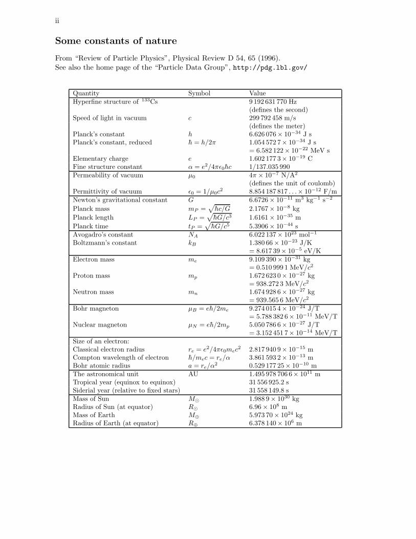
From “Review of Particle Physics”, Physical Review D 54, 65 (1996).See also the home page of the “Particle Data Group”, http://pdg.lbl.gov/
Quantity Symbol ValueHyperfine structure of 133Cs 9 192 631 770 Hz
(defines the second)Speed of light in vacuum c 299 792 458 m/s
(defines the meter)Planck’s constant h 6.626 076× 10−34 J sPlanck’s constant, reduced h = h/2π 1.054 572 7× 10⁻³⁴ J s
= 6.582 122× 10−22 MeV sElementary charge e 1.602 177 3× 10⁻¹⁹ CFine structure constant α = e2/4πǫ0hc 1/137.035 990Permeability of vacuum µ0 4π × 10−7 N/A2
(defines the unit of coulomb)Permittivity of vacuum ǫ0 = 1/µ0c
2 8.854 187 817 . . .× 10−12 F/mNewton’s gravitational constant G 6.6726× 10⁻¹¹ m3 kg−1 s−2
Planck mass mP =√hc/G 2.1767× 10⁻⁸ kg
Planck length LP =√hG/c3 1.6161× 10⁻³⁵ m
Planck time tP =√hG/c5 5.3906× 10−44 s
Avogadro’s constant NA 6.022 137× 1023 mol−1
Boltzmann’s constant kB 1.380 66× 10−23 J/K= 8.617 39× 10−5 eV/K
Electron mass me 9.109 390× 10−31 kg= 0.510 999 1 MeV/c2
Proton mass mp 1.672 623 0× 10−27 kg= 938.272 3 MeV/c2
Neutron mass mn 1.674 928 6× 10⁻²⁷ kg= 939.565 6 MeV/c2
Bohr magneton µB = eh/2me 9.274 015 4× 10⁻²⁴ J/T= 5.788 382 6× 10⁻¹¹ MeV/T
Nuclear magneton µN = eh/2mp 5.050 786 6× 10⁻²⁷ J/T= 3.152 451 7× 10⁻¹⁴ MeV/T
Size of an electron:Classical electron radius re = e2/4πǫ0mec
2 2.817 940 9× 10⁻¹⁵ mCompton wavelength of electron h/mec = re/α 3.861 593 2× 10⁻¹³ mBohr atomic radius a = re/α
2 0.529 177 25× 10−10 mThe astronomical unit AU 1.495 978 706 6× 10¹¹ mTropical year (equinox to equinox) 31 556 925.2 sSiderial year (relative to fixed stars) 31 558 149.8 sMass of Sun M⊙ 1.988 9× 1030 kgRadius of Sun (at equator) R⊙ 6.96 × 10⁸ mMass of Earth M⊕ 5.973 70× 1024 kgRadius of Earth (at equator) R⊕ 6.378 140× 106 m
Contents
Preface i
Some constants of nature ii
1 A brief field guide 11.1 Electromagnetic unit systems . . . . . . . . . . . . . . . . . . . . . . . . . . . 11.2 Index conventions . . . . . . . . . . . . . . . . . . . . . . . . . . . . . . . . . . 21.3 Three dimensional vector notation . . . . . . . . . . . . . . . . . . . . . . . . 31.4 The Dirac δ function . . . . . . . . . . . . . . . . . . . . . . . . . . . . . . . . 51.5 Green functions . . . . . . . . . . . . . . . . . . . . . . . . . . . . . . . . . . . 61.6 Active transformations . . . . . . . . . . . . . . . . . . . . . . . . . . . . . . . 81.7 Passive transformations . . . . . . . . . . . . . . . . . . . . . . . . . . . . . . 12
Problems . . . . . . . . . . . . . . . . . . . . . . . . . . . . . . . . . . . . . . 15
2 Manifolds, vectors and tensors 172.1 The surface of a sphere as an example . . . . . . . . . . . . . . . . . . . . . . 172.2 Manifolds in general . . . . . . . . . . . . . . . . . . . . . . . . . . . . . . . . 192.3 Tensors and tensor fields . . . . . . . . . . . . . . . . . . . . . . . . . . . . . . 232.4 Contravariant vectors . . . . . . . . . . . . . . . . . . . . . . . . . . . . . . . 242.5 Covariant vectors, mixed tensors, and contraction . . . . . . . . . . . . . . . . 282.6 Symmetry and antisymmetry of tensors . . . . . . . . . . . . . . . . . . . . . 302.7 The metric tensor . . . . . . . . . . . . . . . . . . . . . . . . . . . . . . . . . . 31
Problems . . . . . . . . . . . . . . . . . . . . . . . . . . . . . . . . . . . . . . 35
3 Tensor algebra 373.1 Tensor product . . . . . . . . . . . . . . . . . . . . . . . . . . . . . . . . . . . 373.2 Forms and exterior product . . . . . . . . . . . . . . . . . . . . . . . . . . . . 383.3 Tensor densities . . . . . . . . . . . . . . . . . . . . . . . . . . . . . . . . . . . 403.4 Duality . . . . . . . . . . . . . . . . . . . . . . . . . . . . . . . . . . . . . . . 42
Problems . . . . . . . . . . . . . . . . . . . . . . . . . . . . . . . . . . . . . . 44
4 Transformations and Lie algebras 454.1 Infinitesimal coordinate transformations . . . . . . . . . . . . . . . . . . . . . 454.2 Transformations of tensor fields, Lie derivatives . . . . . . . . . . . . . . . . . 474.3 The Lie derivative of a general tensor . . . . . . . . . . . . . . . . . . . . . . . 504.4 Commutation of Lie derivatives . . . . . . . . . . . . . . . . . . . . . . . . . . 514.5 Isometries and Killing vector fields . . . . . . . . . . . . . . . . . . . . . . . . 52
iii

iv CONTENTS
Problems . . . . . . . . . . . . . . . . . . . . . . . . . . . . . . . . . . . . . . 53
5 Differentiation 555.1 Partial and total derivatives . . . . . . . . . . . . . . . . . . . . . . . . . . . . 555.2 Covariant derivatives of tensor fields . . . . . . . . . . . . . . . . . . . . . . . 565.3 Flat and curved space . . . . . . . . . . . . . . . . . . . . . . . . . . . . . . . 585.4 Metric connection . . . . . . . . . . . . . . . . . . . . . . . . . . . . . . . . . . 615.5 Covariant divergence . . . . . . . . . . . . . . . . . . . . . . . . . . . . . . . . 625.6 Exterior derivatives of forms . . . . . . . . . . . . . . . . . . . . . . . . . . . . 635.7 Poincare’s lemma, magnetic monopoles . . . . . . . . . . . . . . . . . . . . . . 645.8 Divergence of densities . . . . . . . . . . . . . . . . . . . . . . . . . . . . . . . 68
Problems . . . . . . . . . . . . . . . . . . . . . . . . . . . . . . . . . . . . . . 70
6 Parallel transport and curvature 716.1 Parallel transport of vectors and tensors . . . . . . . . . . . . . . . . . . . . . 726.2 Covariant differentiation from parallel transport . . . . . . . . . . . . . . . . . 746.3 Torsion and curvature . . . . . . . . . . . . . . . . . . . . . . . . . . . . . . . 756.4 Symmetry properties of the curvature tensor . . . . . . . . . . . . . . . . . . 776.5 Scalar curvature, the Ricci and Weyl tensors . . . . . . . . . . . . . . . . . . 796.6 The Bianchi identity . . . . . . . . . . . . . . . . . . . . . . . . . . . . . . . . 806.7 A method for computing the Ricci tensor . . . . . . . . . . . . . . . . . . . . 81
Problems . . . . . . . . . . . . . . . . . . . . . . . . . . . . . . . . . . . . . . 83
7 Integration 877.1 Line integrals . . . . . . . . . . . . . . . . . . . . . . . . . . . . . . . . . . . . 877.2 Surface integrals . . . . . . . . . . . . . . . . . . . . . . . . . . . . . . . . . . 887.3 Duality . . . . . . . . . . . . . . . . . . . . . . . . . . . . . . . . . . . . . . . 897.4 Length, area and volume . . . . . . . . . . . . . . . . . . . . . . . . . . . . . . 917.5 Differentiation and integration . . . . . . . . . . . . . . . . . . . . . . . . . . 91
Problems . . . . . . . . . . . . . . . . . . . . . . . . . . . . . . . . . . . . . . 94
8 The special theory of relativity 958.1 The speed of light . . . . . . . . . . . . . . . . . . . . . . . . . . . . . . . . . 958.2 The principle of relativity . . . . . . . . . . . . . . . . . . . . . . . . . . . . . 968.3 The Minkowski metric . . . . . . . . . . . . . . . . . . . . . . . . . . . . . . . 968.4 The Poincare group . . . . . . . . . . . . . . . . . . . . . . . . . . . . . . . . 988.5 Continuous Lorentz transformations . . . . . . . . . . . . . . . . . . . . . . . 1008.6 The law of cosmic laziness . . . . . . . . . . . . . . . . . . . . . . . . . . . . . 1058.7 Lorentz contraction . . . . . . . . . . . . . . . . . . . . . . . . . . . . . . . . . 1078.8 Addition of velocities, constant acceleration . . . . . . . . . . . . . . . . . . . 1088.9 Relativistic conservation laws . . . . . . . . . . . . . . . . . . . . . . . . . . . 110
Problems . . . . . . . . . . . . . . . . . . . . . . . . . . . . . . . . . . . . . . 114
9 Particle mechanics 1179.1 Newton’s second law . . . . . . . . . . . . . . . . . . . . . . . . . . . . . . . . 1179.2 Hamilton’s principle . . . . . . . . . . . . . . . . . . . . . . . . . . . . . . . . 1199.3 Hamilton’s equations . . . . . . . . . . . . . . . . . . . . . . . . . . . . . . . . 123
CONTENTS v
9.4 Poisson brackets . . . . . . . . . . . . . . . . . . . . . . . . . . . . . . . . . . 1249.5 Constraints . . . . . . . . . . . . . . . . . . . . . . . . . . . . . . . . . . . . . 1259.6 Equivalent Lagrange functions . . . . . . . . . . . . . . . . . . . . . . . . . . 127
Problems . . . . . . . . . . . . . . . . . . . . . . . . . . . . . . . . . . . . . . 129
10 Symmetries and conservation laws 13110.1 Transformations of space and time . . . . . . . . . . . . . . . . . . . . . . . . 13110.2 Symmetries . . . . . . . . . . . . . . . . . . . . . . . . . . . . . . . . . . . . . 13310.3 Noether’s theorem . . . . . . . . . . . . . . . . . . . . . . . . . . . . . . . . . 13410.4 Examples . . . . . . . . . . . . . . . . . . . . . . . . . . . . . . . . . . . . . . 13410.5 Non-relativistic particles . . . . . . . . . . . . . . . . . . . . . . . . . . . . . . 13610.6 Relativistic particles . . . . . . . . . . . . . . . . . . . . . . . . . . . . . . . . 139
Problems . . . . . . . . . . . . . . . . . . . . . . . . . . . . . . . . . . . . . . 145
11 Field mechanics 14711.1 Hamilton’s principle . . . . . . . . . . . . . . . . . . . . . . . . . . . . . . . . 14711.2 Complex field . . . . . . . . . . . . . . . . . . . . . . . . . . . . . . . . . . . . 15011.3 Hamilton’s equations . . . . . . . . . . . . . . . . . . . . . . . . . . . . . . . . 15111.4 Equivalent Lagrange densities . . . . . . . . . . . . . . . . . . . . . . . . . . . 153
Problems . . . . . . . . . . . . . . . . . . . . . . . . . . . . . . . . . . . . . . 155
12 Symmetries and conservation laws for fields 15712.1 Field transformations . . . . . . . . . . . . . . . . . . . . . . . . . . . . . . . . 15712.2 Symmetries . . . . . . . . . . . . . . . . . . . . . . . . . . . . . . . . . . . . . 15912.3 Noether’s theorem . . . . . . . . . . . . . . . . . . . . . . . . . . . . . . . . . 16012.4 Gauge invariance . . . . . . . . . . . . . . . . . . . . . . . . . . . . . . . . . . 16112.5 Translation invariance . . . . . . . . . . . . . . . . . . . . . . . . . . . . . . . 16212.6 Lorentz invariance . . . . . . . . . . . . . . . . . . . . . . . . . . . . . . . . . 16312.7 Symmetrization of the energy momentum tensor . . . . . . . . . . . . . . . . 166
Problems . . . . . . . . . . . . . . . . . . . . . . . . . . . . . . . . . . . . . . 168
13 The Klein–Gordon field 17113.1 Lagrange formalism . . . . . . . . . . . . . . . . . . . . . . . . . . . . . . . . 17213.2 Plane wave solutions and quantization . . . . . . . . . . . . . . . . . . . . . . 17313.3 The Yukawa potential . . . . . . . . . . . . . . . . . . . . . . . . . . . . . . . 17513.4 Interaction of particles and fields . . . . . . . . . . . . . . . . . . . . . . . . . 17713.5 Electrically charged Klein–Gordon field . . . . . . . . . . . . . . . . . . . . . 18113.6 Klein–Gordon field in an external gravitational field . . . . . . . . . . . . . . 183
Problems . . . . . . . . . . . . . . . . . . . . . . . . . . . . . . . . . . . . . . 185
14 The Maxwell field 18714.1 Maxwell’s equations . . . . . . . . . . . . . . . . . . . . . . . . . . . . . . . . 18814.2 Lagrange formalism . . . . . . . . . . . . . . . . . . . . . . . . . . . . . . . . 19114.3 Energy momentum tensor . . . . . . . . . . . . . . . . . . . . . . . . . . . . . 19414.4 Plane wave solutions . . . . . . . . . . . . . . . . . . . . . . . . . . . . . . . . 19614.5 Interaction of particles and fields . . . . . . . . . . . . . . . . . . . . . . . . . 19814.6 Maxwell’s equations in an external gravitational field . . . . . . . . . . . . . . 200
vi CONTENTS
14.7 Duality between electric and magnetic fields . . . . . . . . . . . . . . . . . . . 201Problems . . . . . . . . . . . . . . . . . . . . . . . . . . . . . . . . . . . . . . 204
15 Gravitation and geometry 20515.1 The principle of equivalence . . . . . . . . . . . . . . . . . . . . . . . . . . . . 20615.2 Non-relativistic limit . . . . . . . . . . . . . . . . . . . . . . . . . . . . . . . . 20815.3 Gravitational redshift . . . . . . . . . . . . . . . . . . . . . . . . . . . . . . . 20915.4 The equation of motion for a point mass . . . . . . . . . . . . . . . . . . . . . 20915.5 Tidal forces due to geodesic deviation . . . . . . . . . . . . . . . . . . . . . . 211
Problems . . . . . . . . . . . . . . . . . . . . . . . . . . . . . . . . . . . . . . 215
16 Einstein’s gravitational equation 21716.1 Einstein’s field equation . . . . . . . . . . . . . . . . . . . . . . . . . . . . . . 21716.2 Static mass distribution and weak field . . . . . . . . . . . . . . . . . . . . . . 21916.3 Deflection of light . . . . . . . . . . . . . . . . . . . . . . . . . . . . . . . . . . 22116.4 Linearized gravitational theory . . . . . . . . . . . . . . . . . . . . . . . . . . 22416.5 The geodesic equation follows from the field equation . . . . . . . . . . . . . . 22516.6 The cosmological constant . . . . . . . . . . . . . . . . . . . . . . . . . . . . . 226
Problems . . . . . . . . . . . . . . . . . . . . . . . . . . . . . . . . . . . . . . 228
17 Lagrange formalism for the gravitational field 22917.1 Hilbert’s variational principle . . . . . . . . . . . . . . . . . . . . . . . . . . . 22917.2 Palatini’s variational principle . . . . . . . . . . . . . . . . . . . . . . . . . . . 23117.3 Uniqueness of Einstein’s gravitational equation . . . . . . . . . . . . . . . . . 233
Problems . . . . . . . . . . . . . . . . . . . . . . . . . . . . . . . . . . . . . . 238
18 Rotationally symmetric gravitational field 23918.1 Spherically symmetric metric . . . . . . . . . . . . . . . . . . . . . . . . . . . 23918.2 The Ricci tensor . . . . . . . . . . . . . . . . . . . . . . . . . . . . . . . . . . 24118.3 The Schwarzschild metric . . . . . . . . . . . . . . . . . . . . . . . . . . . . . 24318.4 Planetary orbits . . . . . . . . . . . . . . . . . . . . . . . . . . . . . . . . . . 24518.5 Generalizations of the Schwarzschild metric . . . . . . . . . . . . . . . . . . . 25018.6 Black and white holes . . . . . . . . . . . . . . . . . . . . . . . . . . . . . . . 25218.7 Hawking radiation, or grey, red and blue holes . . . . . . . . . . . . . . . . . 257
Problems . . . . . . . . . . . . . . . . . . . . . . . . . . . . . . . . . . . . . . 260
19 Cosmology 26119.1 Observational basis . . . . . . . . . . . . . . . . . . . . . . . . . . . . . . . . . 26219.2 The metric . . . . . . . . . . . . . . . . . . . . . . . . . . . . . . . . . . . . . 26519.3 The energy momentum tensor . . . . . . . . . . . . . . . . . . . . . . . . . . . 26919.4 The Ricci tensor . . . . . . . . . . . . . . . . . . . . . . . . . . . . . . . . . . 27519.5 The gravitational equation . . . . . . . . . . . . . . . . . . . . . . . . . . . . . 27819.6 Solutions of the gravitational equation . . . . . . . . . . . . . . . . . . . . . . 28219.7 Nucleosynthesis . . . . . . . . . . . . . . . . . . . . . . . . . . . . . . . . . . . 284
Problems . . . . . . . . . . . . . . . . . . . . . . . . . . . . . . . . . . . . . . 288
A A simple Maple program for differential geometry 289
CONTENTS vii
B Group theory 295B.1 The group axioms . . . . . . . . . . . . . . . . . . . . . . . . . . . . . . . . . 295B.2 Examples . . . . . . . . . . . . . . . . . . . . . . . . . . . . . . . . . . . . . . 299B.3 Lie groups . . . . . . . . . . . . . . . . . . . . . . . . . . . . . . . . . . . . . . 301B.4 Lie algebras . . . . . . . . . . . . . . . . . . . . . . . . . . . . . . . . . . . . . 304B.5 Examples . . . . . . . . . . . . . . . . . . . . . . . . . . . . . . . . . . . . . . 305
C Statistical mechanics 307
Index 313

viii CONTENTS

Chapter 1
A brief field guide
This first chapter is an assorted collection of notes on units, notation etc., which may be usedas a field guide to be consulted whenever needed. The immediately following chapters give abrief introduction to differential geometry, which is the mathematics of classical field theoryin general, and of the general theory of relativity in particular.
It is certainly possible to read the first chapters as a mathematics text book, before movingon to the physical applications. However, since the physics motivates the mathematics, somereaders may prefer to start with Chapter 8, on the special theory of relativity, and to use allthe mathematical chapters as a field guide.
1.1 Electromagnetic unit systems
We use here SI units, also called MKSA units: meter, kilogram, second and ampere. Unfortu-nately, this is only one out of at least three different electromagnetic unit systems in commonuse, the other two being Gaussian and Heaviside–Lorentz units. The differences show up inCoulomb’s law for the potential energy V between two point charges q1 and q2 at a relativedistance r,
V = kq1q2r
. (1.1)
The proportionality constant k is different in the three unit systems,
k =1
4πǫ0in SI units;
k = 1 in Gaussian units;
k =1
4πin Heaviside–Lorentz units.
The fine structure constant α, given by the elementary charge e, the reduced Planck’s constanth and the speed of light c, has the same numerical value in the three unit systems,
α = ke2
hc=
1
137.035 990. (1.2)
The second place where differences show up is in the expression for the Lorentz force on anelectric point charge q moving with a velocity v in an electromagnetic field in vacuum,
1
2 CHAPTER 1. A BRIEF FIELD GUIDE
F = q (E + v × B) (SI); (1.3)
F = q
(E +
v
c× B
)(Gauss or Heaviside–Lorentz).
Here E is the electric field and B the magnetic flux density at the point where the charge islocated. As can be seen, E and B have the same dimension in Gaussian units, and also inHeaviside–Lorentz units, whereas an expression like |E|/|B| has the dimension of velocity inthe SI system.
1.2 Index conventions
We use greek letters α, β, µ, ν, . . . as indices to enumerate time and space coordinates. Theyrun then from 0 to 3, and the time coordinate is usually labelled 0. Spatial coordinates alonewe enumerate with latin indices i, j, . . ., running from 1 to 3, or more generally from 1 tod, where d is the dimension. We use latin indices in most other cases, e.g. for enumeratinggeneralized coordinates in Lagrangian mechanics, or field componentes.
Unless stated otherwise, we use the summation convention that an index occurring twicein a product is to be summed over. In tensor expressions, the summation index normallyoccurs as an upper and a lower index, otherwise the sum may depend on which coordinatesystem is used.
The Kronecker δ symbol
This has two indices that may be latin or greek, upper or lower, depending on the context.By definition,
δij = δij = δij =
1 when i = j,0 when i 6= j.
(1.4)
The Levi–Civita symbol
In an n dimensional space, the Levi–Civita symbol ǫµν...σ has n indices, and is antisymmetricunder an interchange of any two indices. The number of components is nn. Any componentwith two indices taking the same value must vanish because of the antisymmetry. Of the n!components whose n indices take n different values, half are +1 and the other half −1. Wedefine here the Levi–Civita symbols with upper and lower indices to be equal, ǫµν...σ = ǫµν...σ.
The determinant det(A) of an n× n matrix A may be defined by the relation
ǫκλ...νAακA
βλ · · ·Aδ
ν = det(A) ǫαβ...δ . (1.5)
In fact, the left hand side of this equation must be proportional to ǫαβ...δ, because it is totallyantisymmetric in the indices α, β, . . . , δ. The proportionality constant is the determinant.
The Levi–Civita symbol in a two dimensional space, as an example, has 22 = 4 compo-nents,
ǫ12 = −ǫ21 = 1 , ǫ11 = ǫ22 = 0 , (1.6)

1.3. THREE DIMENSIONAL VECTOR NOTATION 3
and we see that
ǫklAikA
jl = Ai
1Aj2 −Ai
2Aj1 = (A1
1A22 −A1
2A21) ǫ
ij = det(A) ǫij . (1.7)
In three dimensions the number of components is 33 = 27, and we have
ǫ123 = ǫ231 = ǫ312 = −ǫ213 = −ǫ132 = −ǫ321 = 1 , all other ǫijk = 0 . (1.8)
In the four dimensional spacetime, the number of components is 44 = 256, all determined bythe antisymmetry and by the definition ǫ0123 = 1.
Note that the convention used here, that ǫµν...σ = ǫµν...σ, differs from a convention fre-quently used in the special theory of relativity, that ǫµνρσ = −ǫµνρσ. The last convention isnatural if ǫµνρσ is regarded as a tensor. Then the factor −1 appearing when the indices arelowered, is the determinant of the metric tensor. In the general theory of relativity, on theother hand, where the metric tensor is more freely variable and may have a determinant dif-ferent from −1, it seems natural to define the Levi–Civita symbol independently of the metrictensor. Under a coordinate transformation which does not preserve volume, the Levi–Civitasymbol, as defined here, transforms not as a tensor but as a tensor density, as defined inChapter 3.
1.3 Three dimensional vector notation
In three dimensional Euclidean space we use a special vector notation, exemplified below.When indices are occasionally used, they are always written as lower latin indices. An indexoccurring twice in a product is to be summed over, but summing over two lower indices meansthat a formula is valid only in Euclidean coordinate systems, where the metric tensor equalsthe identity matrix, gij = δij. The examples will demonstrate the rules.
– Standard unit vectors: i = ex = e1 , j = ey = e2 , k = ez = e3 .
– Position vector: r = x i + y j + z k = x1 e1 + x2 e2 + x3 e3 = xi ei ,differential: dr = dx i + dy j + dz k .
– General vector: A = Ax i +Ay j +Az k = A1 e1 +A2 e2 +A3 e3 = Ai ei .
– Scalar product between vectors: A · B = AxBx +AyBy +AzBz = AiBi ,and in particular: |A|2 = A2 = A · A = Ax
2 +Ay2 +Az
2 = AiAi .
– Vector product: A × B = (AyBz −AzBy) i + (AzBx −AxBz) j + (AxBy −AyBx)k ,in index notation: (A × B)i = ǫijkAjBk .
– Metric: ds2 = |dr|2 = dr2 = dr · dr = dx2 + dy2 + dz2 .
– Volume element: dV = d3r = dxdy dz .
– Nabla, the gradient operator:
∇ =∂
∂r= i
∂
∂x+ j
∂
∂y+ k
∂
∂z. (1.9)
– Laplace operator:
∆ = ∇2 = ∇ · ∇ =∂2
∂x2+
∂2
∂y2+
∂2
∂z2. (1.10)
4 CHAPTER 1. A BRIEF FIELD GUIDE
Example: Polar coordinates
The polar coordinates (r, θ, ϕ) are related to the Euclidean coordinates (x, y, z) by the for-mulae
x = r sin θ cosϕ , y = r sin θ sinϕ , z = r cos θ . (1.11)
The definition gives, by the chain rule for differentiation, that
dr = dr∂r
∂r+ dθ
∂r
∂θ+ dϕ
∂r
∂ϕ= dr er + r dθ eθ + r sin θ dϕ eϕ , (1.12)
when we introduce the basis vectors
er =∂r
∂r= sin θ cosϕ i + sin θ sinϕ j + cos θ k ,
eθ =1
r
∂r
∂θ= cos θ cosϕ i + cos θ sinϕ j − sin θ k , (1.13)
eϕ =1
r sin θ
∂r
∂ϕ= − sinϕ i + cosϕ j ,
which are orthonormal, i.e. they are orthogonal unit vectors,
ei · ej = δij , with i, j = r, θ, ϕ . (1.14)
It follows that
dr2 = dr2 + r2dθ2 + r2 sin2θ dϕ2 . (1.15)
Let f = f(r). Then we have, according to the chain rule for differentiation, that
∂f
∂r=∂r
∂r· ∂f∂r
= er · ∇f ,∂f
∂θ=∂r
∂θ· ∂f∂r
= r eθ · ∇f , (1.16)
∂f
∂ϕ=
∂r
∂ϕ· ∂f∂r
= r sin θ eϕ · ∇f .
Consequently, we have
∇f = er (er · ∇f) + eθ (eθ · ∇f) + eϕ (eϕ · ∇f)
= er∂f
∂r+ eθ
1
r
∂f
∂θ+ eϕ
1
r sin θ
∂f
∂ϕ, (1.17)
which may also be written as follows,
∇ = er∂
∂r+ eθ
1
r
∂
∂θ+ eϕ
1
r sin θ
∂
∂ϕ. (1.18)
1.4. THE DIRAC δ FUNCTION 5
1.4 The Dirac δ function
The Dirac δ function is the generalization of the Kronecker symbol δij to the case when theindices i and j are continuous variables. The one dimensional δ function is defined by therelation ∫ ∞
−∞dx δ(x− y) f(x) = f(y) , (1.19)
valid for an arbitrary continuous function f = f(x). The δ function is symmetric, δ(x− y) =δ(y − x), because the substitution u = −x gives that
∫ ∞
−∞dx δ(y − x) f(x) =
∫ ∞
−∞du δ(y + u) f(−u) = f(y) . (1.20)
More generally we have that
δ(ax) =1
|a| δ(x) (1.21)
when a is constant, a 6= 0, since the substitution u = |a|x gives that∫ ∞
−∞dx δ(ax) f(x) =
1
|a|
∫ ∞
−∞du δ(±u) f
(u
|a|
)=
1
|a| f(0) . (1.22)
Even more generally, when g is a differentiable function with g(0) = 0, with g(x) = 0 only forx = 0, and with g′(0) 6= 0, we will have that
δ(g(x)) =1
|g′(0)| δ(x) (1.23)
The derivatives of the δ function may be defined formally in the usual way,
δ′(x) = limh→0
δ(x + h) − δ(x − h)
2h, (1.24)
δ′′(x) = limh→0
δ(x + h) + δ(x − h) − 2δ(x)
h2.
This then gives that∫ ∞
−∞dx δ′(x− y) f(x) = lim
h→0
f(y − h) − f(y + h)
2h= −f ′(y) , (1.25)
∫ ∞
−∞dx δ′′(x− y) f(x) = lim
h→0
f(y − h) + f(y + h) − 2f(y)
h2= f ′′(y) .
These results can alternatively be derived by partial integrations, for example,∫ ∞
−∞dx δ′(x− y) f(x) = −
∫ ∞
−∞dx δ(x − y) f ′(x) = −f ′(y) . (1.26)
The δ functions in higher dimensions can be defined in a similar way, for example in threedimensions,
∫d3r δ(3)(r − s) f(r) = f(s) . (1.27)
The three dimensional δ function is written as δ(3)(r), or simply as δ(r) if there is no dangerof confusion. It is the product of one dimensional δ functions,
δ(r) = δ(x) δ(y) δ(z) . (1.28)
6 CHAPTER 1. A BRIEF FIELD GUIDE
1.5 Green functions
Take an inhomogeneous differential equation, with boundary conditions that make the solu-tion uniquely defined. For example the Poisson equation in three dimensions,
∇2f = g , (1.29)
where f = f(r) is an unknown function satisfying the boundary condition that f(r) → 0 as|r| → ∞. The right hand side of the equation, the known source g = g(r), is assumed to belocalized, so that it vanishes outside some region of finite extent.
Then the Green function of this equation with boundary conditions is the solution f inthe case when the source g is the Dirac δ function. To be more precise, the Green functionG = G(r; s) is a function of two points r and s such that G(r; s) → 0 when |r| → ∞, and
∇2G(r; s) = δ(r − s) , (1.30)
where the Laplace operator ∇2 differentiates with respect to r. The Green function of thePoisson equation gives the solution for a general right hand side g as
f(r) =
∫d3sG(r; s) g(s) , (1.31)
as we can see directly by substitution into the equation. Thus, the operation g 7→ f definedby this integral, is the inverse of the operation f 7→ g = ∇2f .
In our example here we have G(r; s) = G(r − s), where G = G(r) is the solution of theequation
∇2G = δ . (1.32)
This simplification is possible because of the translational symmetry of the Poisson equation.Rotational symmetry implies the further simplification that G = G(r) is a function of theradius r = |r| alone, that is, G = G(r).
One method for solving the equation ∇2G = δ is to integrate over a volume V which is asphere with centre at the origin and radius R > 0. The integral of the left hand side is, bythe divergence theorem, equal to a surface integral over the surface S of the sphere,
∫
VdV ∇2G =
∫
SdS er · ∇G = 4πR2G′(R) . (1.33)
Here er = r/r is the unit vector in the radial direction. The integral of the right hand side is
∫
VdV δ(r) = 1 . (1.34)
Equating the two integrals gives the differential equation
G′(R) =1
4πR2. (1.35)
With the boundary condition G(R) → 0 as R→ ∞ the solution is
G(R) = − 1
4πR. (1.36)

1.5. GREEN FUNCTIONS 7
Thus we find the Green function
G(r; s) = G(|r − s|) = − 1
4π|r − s| . (1.37)
In this result we recognize the Coulomb potential. The Green function for the Poisson equa-tion is the electrostatic potential of a unit point charge.
A second method for solving the same equation is the following Fourier transformation,
f(r) =
∫d3k f(k) e−ik·r , g(r) =
∫d3k g(k) e−ik·r . (1.38)
It implies that
∇2f(r) = −∫
d3k |k|2 f(k) e−ik·r . (1.39)
The inverse Fourier transformation gives that
g(k) =1
(2π)3
∫d3r g(r) eik·r . (1.40)
Thus, the Fourier transformed differential equation ∇2G = δ is the simple algebraic equation
−|k|2 G(k) =1
(2π)3. (1.41)
We see that the Fourier transform of the Green function, G = G(k), becomes singular atk = 0. A trick for avoiding this singularity is to solve instead the modified equation
∇2G− κ2G = δ , (1.42)
with κ > 0, and afterwards let κ→ 0+. The Green function of the modified equation is
Gκ(r) = − 1
(2π)3
∫d3k
e−ik·r
|k|2 + κ2(1.43)
= − 1
(2π)3
∫ ∞
0k2 dk
∫ 1
−1d(cos θ)
∫ 2π
0dϕ
e−ikr cos θ
k2 + κ2.
Here k = |k|, and we define θ and ϕ as the polar angles of the vector k relative to an axisalong r, so that k · r = kr cos θ. After performing the angular integrations, we get that
Gκ(r) = Gκ(r) = − 1
(2π)2
∫ ∞
0dk
k2
k2 + κ2
(−e−ikr
ikr+
eikr
ikr
)
=i
(2π)2 r
∫ ∞
−∞dk
k eikr
k2 + κ2. (1.44)
In the last integral, the integration contour along the real axis can be closed in the complexplane by a half circle of infinite radius in the upper half plane. The half circle does notcontribute to the integral, because the integrand vanishes rapidly in the limit k → ∞, when
8 CHAPTER 1. A BRIEF FIELD GUIDE
k is complex with a positive imaginary part. The integrand has one single pole in the upperhalf plane, at k = iκ, and the residue of the pole is
limk→iκ
(k − iκ)k eikr
k2 + κ2=
1
2e−κr . (1.45)
The value of the integral is 2πi times the residue. Hence,
Gκ(r) = Gκ(r) =i
(2π)2 r2πi
1
2e−κr = −e−κr
4πr. (1.46)
This is the Yukawa potential, which is the static solution of the Klein–Gordon equation witha δ function source, and which has the Coulomb potential as its limit when κ→ 0+.
1.6 Active transformations
In order to be concrete we will talk here mostly about transformations of fields, even thoughmuch of what is said is more generally valid. We distinguish between active transforma-tions, transforming the field, and passive transformations, transforming the coordinate sys-tem without transforming the field. A passive transformation is no more than a coordinatetransformation, by which the same field is described relative to a new coordinate system.The mathematical description of active and passive transformations is exactly the same, andtherefore we often do not bother to specify whether the transformation equations should beinterpreted actively or passively.
An active transformation transforms one field configuration into another. We call it a sym-metry of the system if it is invertible, so that it can be undone by some inverse transformation,and if in addition it preserves the field equation. Which means that the transformed fieldconfiguration is a solution of the field equation if and only if the original field configurationis a solution.
This definition implies that if a given transformation is a symmetry, then so is the inversetransformation. It implies furthermore that a composite transformation consisting of firstone and then a second symmetry transformation, is again a symmetry. These two propertiesmean, in the language of mathematics, that the symmetries of a given physical system forma group.
Example: Translation
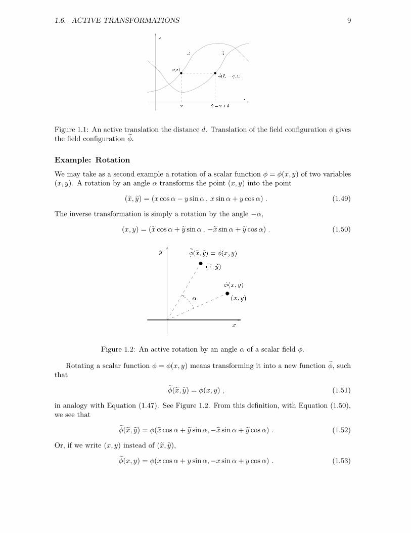
An example of an active transformation is a translation, or displacement, of a scalar functionφ = φ(x) of one variable x.
Displacing the whole function a constant distance d, means moving the function valueφ(x) from a given point x to a new point x = x+ d. That is, we define a new function φ suchthat
φ(x) = φ(x) . (1.47)
See Figure 1.1. The transformation equation φ(x + d) = φ(x) means that the transformedfunction φ is defined by the equation
φ(x) = φ(x− d) . (1.48)
1.6. ACTIVE TRANSFORMATIONS 9
x
ex = x+ d xe(ex) = (x)e(x)Figure 1.1: An active translation the distance d. Translation of the field configuration φ givesthe field configuration φ.
Example: Rotation
We may take as a second example a rotation of a scalar function φ = φ(x, y) of two variables(x, y). A rotation by an angle α transforms the point (x, y) into the point
(x, y) = (x cosα− y sinα , x sinα+ y cosα) . (1.49)
The inverse transformation is simply a rotation by the angle −α,
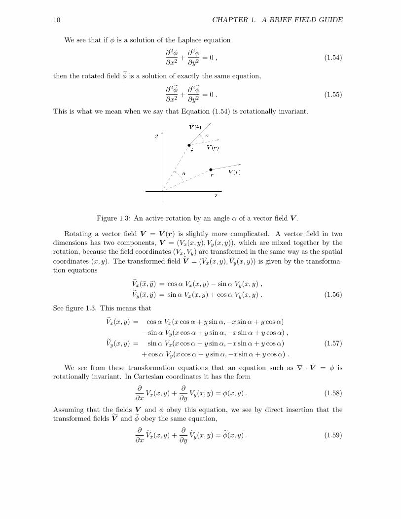
(x, y) = (x cosα+ y sinα , −x sinα+ y cosα) . (1.50) (x; y)e(ex; ey) = (x; y)y x(ex; ey) (x; y)Figure 1.2: An active rotation by an angle α of a scalar field φ.
Rotating a scalar function φ = φ(x, y) means transforming it into a new function φ, suchthat
φ(x, y) = φ(x, y) , (1.51)
in analogy with Equation (1.47). See Figure 1.2. From this definition, with Equation (1.50),we see that
φ(x, y) = φ(x cosα+ y sinα,−x sinα+ y cosα) . (1.52)
Or, if we write (x, y) instead of (x, y),
φ(x, y) = φ(x cosα+ y sinα,−x sinα+ y cosα) . (1.53)
10 CHAPTER 1. A BRIEF FIELD GUIDE
We see that if φ is a solution of the Laplace equation
∂2φ
∂x2+∂2φ
∂y2= 0 , (1.54)
then the rotated field φ is a solution of exactly the same equation,
∂2φ
∂x2+∂2φ
∂y2= 0 . (1.55)
This is what we mean when we say that Equation (1.54) is rotationally invariant.
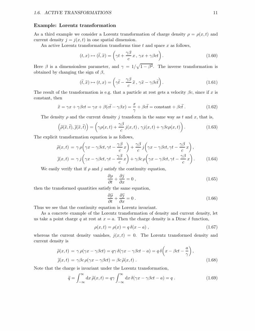
y x rer V (r)V (r)fV (er)Figure 1.3: An active rotation by an angle α of a vector field V .
Rotating a vector field V = V (r) is slightly more complicated. A vector field in twodimensions has two components, V = (Vx(x, y), Vy(x, y)), which are mixed together by therotation, because the field coordinates (Vx, Vy) are transformed in the same way as the spatial
coordinates (x, y). The transformed field V = (Vx(x, y), Vy(x, y)) is given by the transforma-tion equations
Vx(x, y) = cosα Vx(x, y) − sinα Vy(x, y) ,
Vy(x, y) = sinα Vx(x, y) + cosα Vy(x, y) . (1.56)
See figure 1.3. This means that
Vx(x, y) = cosα Vx(x cosα+ y sinα,−x sinα+ y cosα)
− sinα Vy(x cosα+ y sinα,−x sinα+ y cosα) ,
Vy(x, y) = sinα Vx(x cosα+ y sinα,−x sinα+ y cosα) (1.57)
+ cosα Vy(x cosα+ y sinα,−x sinα+ y cosα) .
We see from these transformation equations that an equation such as ∇ · V = φ isrotationally invariant. In Cartesian coordinates it has the form
∂
∂xVx(x, y) +
∂
∂yVy(x, y) = φ(x, y) . (1.58)
Assuming that the fields V and φ obey this equation, we see by direct insertion that thetransformed fields V and φ obey the same equation,
∂
∂xVx(x, y) +
∂
∂yVy(x, y) = φ(x, y) . (1.59)
1.6. ACTIVE TRANSFORMATIONS 11
Example: Lorentz transformation
As a third example we consider a Lorentz transformation of charge density ρ = ρ(x, t) andcurrent density j = j(x, t) in one spatial dimension.
An active Lorentz transformation transforms time t and space x as follows,
(t, x) 7→ (t, x) =
(γt+
γβ
cx , γx+ γβct
). (1.60)
Here β is a dimensionless parameter, and γ = 1/√
1 − β2. The inverse transformation isobtained by changing the sign of β,
(t, x) 7→ (t, x) =
(γt− γβ
cx , γx− γβct
). (1.61)
The result of the transformation is e.g. that a particle at rest gets a velocity βc, since if x isconstant, then
x = γx+ γβct = γx+ β(ct− γβx) =x
γ+ βct = constant + βct . (1.62)
The density ρ and the current density j transform in the same way as t and x, that is,(ρ(x, t), (x, t)
)=
(γρ(x, t) +
γβ
cj(x, t) , γj(x, t) + γβcρ(x, t)
). (1.63)
The explicit transformation equation is as follows,
ρ(x, t) = γ ρ
(γx− γβct, γt− γβ
cx
)+γβ
cj
(γx− γβct, γt− γβ
cx
),
(x, t) = γ j
(γx− γβct, γt− γβ
cx
)+ γβc ρ
(γx− γβct, γt− γβ
cx
). (1.64)
We easily verify that if ρ and j satisfy the continuity equation,
∂ρ
∂t+∂j
∂x= 0 , (1.65)
then the transformed quantities satisfy the same equation,
∂ρ
∂t+∂
∂x= 0 . (1.66)
Thus we see that the continuity equation is Lorentz invariant.As a concrete example of the Lorentz transformation of density and current density, let
us take a point charge q at rest at x = a. Then the charge density is a Dirac δ function,
ρ(x, t) = ρ(x) = q δ(x − a) , (1.67)
whereas the current density vanishes, j(x, t) = 0. The Lorentz transformed density andcurrent density is
ρ(x, t) = γ ρ(γx− γβct) = qγ δ(γx − γβct− a) = q δ
(x− βct− a
γ
),
(x, t) = γβc ρ(γx− γβct) = βc ρ(x, t) . (1.68)
Note that the charge is invariant under the Lorentz transformation,
q =
∫ ∞
−∞dx ρ(x, t) = qγ
∫ ∞
−∞dx δ(γx− γβct− a) = q . (1.69)
12 CHAPTER 1. A BRIEF FIELD GUIDE
1.7 Passive transformations
As already stated, a passive transformation is just a coordinate transformation. It is a symme-try of the system if the transformed field equation has the same form as the original equation.However, this definition of a symmetry is vacuous until we define what we mean by the state-ment that two equations have the same form. We could always define that the transformedequation is the same as the original, only expressed in a different coordinate system. Clearlysuch an all embracing definition, that all field equations are invariant under all coordinatetransformations, is not very interesting, and we are usually much more restrictive.
Example: Rotation
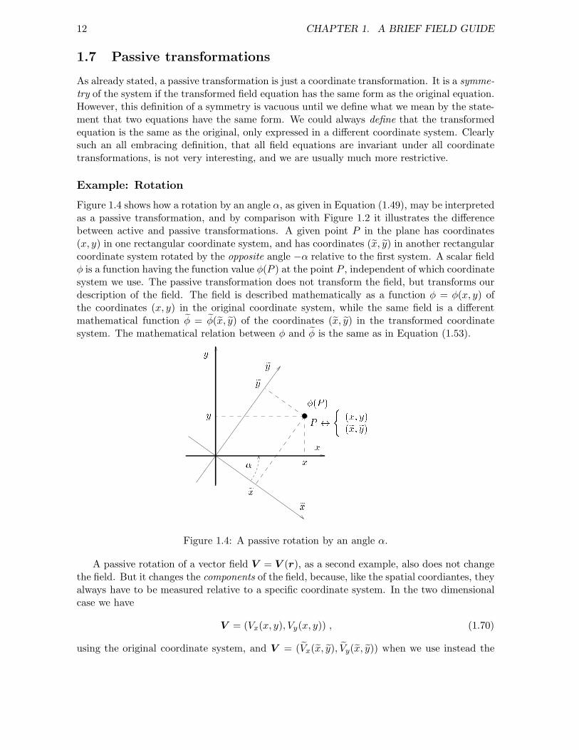
Figure 1.4 shows how a rotation by an angle α, as given in Equation (1.49), may be interpretedas a passive transformation, and by comparison with Figure 1.2 it illustrates the differencebetween active and passive transformations. A given point P in the plane has coordinates(x, y) in one rectangular coordinate system, and has coordinates (x, y) in another rectangularcoordinate system rotated by the opposite angle −α relative to the first system. A scalar fieldφ is a function having the function value φ(P ) at the point P , independent of which coordinatesystem we use. The passive transformation does not transform the field, but transforms ourdescription of the field. The field is described mathematically as a function φ = φ(x, y) ofthe coordinates (x, y) in the original coordinate system, while the same field is a differentmathematical function φ = φ(x, y) of the coordinates (x, y) in the transformed coordinatesystem. The mathematical relation between φ and φ is the same as in Equation (1.53).y
xex(P )eyy ey P $ ( (x; y)(ex; ey)xexFigure 1.4: A passive rotation by an angle α.
A passive rotation of a vector field V = V (r), as a second example, also does not changethe field. But it changes the components of the field, because, like the spatial coordiantes, theyalways have to be measured relative to a specific coordinate system. In the two dimensionalcase we have
V = (Vx(x, y), Vy(x, y)) , (1.70)
using the original coordinate system, and V = (Vx(x, y), Vy(x, y)) when we use instead the
1.7. PASSIVE TRANSFORMATIONS 13
transformed coordinate system. We write
V = (Vx(x, y), Vy(x, y)) , (1.71)
with the implicit understanding that V and V represent the same field as described in two dif-ferent coordinate systems. The mathematical transformation equation is still Equation (1.56),exactly as in the active case.
Example: Polar coordinates in the plane
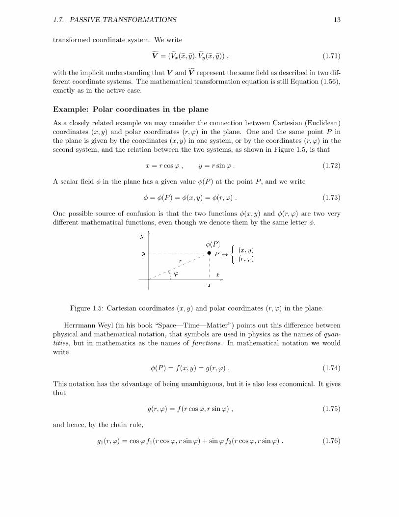
As a closely related example we may consider the connection between Cartesian (Euclidean)coordinates (x, y) and polar coordinates (r, ϕ) in the plane. One and the same point P inthe plane is given by the coordinates (x, y) in one system, or by the coordinates (r, ϕ) in thesecond system, and the relation between the two systems, as shown in Figure 1.5, is that
x = r cosϕ , y = r sinϕ . (1.72)
A scalar field φ in the plane has a given value φ(P ) at the point P , and we write
φ = φ(P ) = φ(x, y) = φ(r, ϕ) . (1.73)
One possible source of confusion is that the two functions φ(x, y) and φ(r, ϕ) are two verydifferent mathematical functions, even though we denote them by the same letter φ.xy x(P )P $ ( (x; y)(r; ')'ry
Figure 1.5: Cartesian coordinates (x, y) and polar coordinates (r, ϕ) in the plane.
Herrmann Weyl (in his book “Space—Time—Matter”) points out this difference betweenphysical and mathematical notation, that symbols are used in physics as the names of quan-tities, but in mathematics as the names of functions. In mathematical notation we wouldwrite
φ(P ) = f(x, y) = g(r, ϕ) . (1.74)
This notation has the advantage of being unambiguous, but it is also less economical. It givesthat
g(r, ϕ) = f(r cosϕ, r sinϕ) , (1.75)
and hence, by the chain rule,
g1(r, ϕ) = cosϕf1(r cosϕ, r sinϕ) + sinϕf2(r cosϕ, r sinϕ) . (1.76)
14 CHAPTER 1. A BRIEF FIELD GUIDE
Here g1 = ∂g/∂r is the derivative of g with respect to its first argument, and similarlyf1 = ∂f/∂x and f2 = ∂f/∂y. In “physicist notation” we would write the same equationsimply as
∂φ
∂r=∂x
∂r
∂φ
∂x+∂y
∂r
∂φ
∂y= cosϕ
∂φ
∂x+ sinϕ
∂φ
∂y. (1.77)
This notation is usually sufficiently unambiguous, but in order to make it totally unambiguousone must specify explicitly what is constant during differentiation, in the following way,
∂φ
∂r
∣∣∣∣ϕ
=∂x
∂r
∣∣∣∣ϕ
∂φ
∂x
∣∣∣∣y
+∂y
∂r
∣∣∣∣ϕ
∂φ
∂y
∣∣∣∣x
. (1.78)
Thus, at the one point P = (x, y) = (r, ϕ), with two different coordinate systems we havefour different partial derivatives, standing in the following relations,
∂
∂r=∂x
∂r
∂
∂x+∂y
∂r
∂
∂y= cosϕ
∂
∂x+ sinϕ
∂
∂y,
∂
∂ϕ=
∂x
∂ϕ
∂
∂x+∂y
∂ϕ
∂
∂y= −r sinϕ
∂
∂x+ r cosϕ
∂
∂y, (1.79)
and conversely,
∂
∂x=
∂r
∂x
∂
∂r+∂ϕ
∂x
∂
∂ϕ= cosϕ
∂
∂r− sinϕ
r
∂
∂ϕ,
∂
∂y=
∂r
∂y
∂
∂r+∂ϕ
∂y
∂
∂ϕ= sinϕ
∂
∂r+
cosϕ
r
∂
∂ϕ. (1.80)
We have the following expressions for the Laplace operator ∇2 in the two coordinate systems,
∇2 =∂2
∂x2+
∂2
∂y2=
∂2
∂r2+
1
r
∂
∂r+
1
r2∂2
∂ϕ2. (1.81)
One would ordinarily tend to say that the two equations
∂2φ
∂x2+∂2φ
∂y2= 0 (1.82)
and
∂2φ
∂r2+
1
r
∂φ
∂r+
1
r2∂2φ
∂ϕ2= 0 (1.83)
are not of the same form. But this question is very much a matter of definition, since itis equally natural to see the two equations as just the same equation, the Laplace equation∇2φ = 0, expressed in two different coordinate systems.
1.7. PASSIVE TRANSFORMATIONS 15
Problems
1. Use Equation (1.18) to express the Laplace operator ∇2 in polar coordinates. That is,compute ∇2f = ∇ · (∇f) for an arbitrary function f . Remember to differentiate theunit vectors er, eθ and eϕ.
2. We say that a scalar function φ = φ(x) in one dimension is invariant under translationa distance d if φ(x) = φ(x − d). This means that the translated function φ as definedin Equation (1.48) is equal to the original function φ.Precisely which functions are invariant under translation a fixed distance d?Which functions are translationally invariant, in the sense that they are invariant undertranslation a distance d simultaneously for all values of d?
3. Similarly, we say that a scalar function (scalar field) φ = φ(x, y) in two dimensions isinvariant under rotation by a fixed angle α if φ = φ in Equation (1.53). We say simplythat φ is invariant under rotations, or rotationally invariant, if it is invariant underrotation by any angle α.Precisely which scalar functions in two dimensions are invariant under rotation by afixed angle α? (This question is actually somewhat tricky, and the answer depends onwhether α is a rational or irrational multiple of π.)Which scalar functions in two dimensions are rotationally invariant?
4. Explain (for example by drawing a sketch) what the most general rotationally invariantvector field in the plane must look like. Again, “rotationally invariant” means “invariantunder rotation by an arbitrary angle”.What can you say about the value at the origin of a rotationally invariant vector field?

16 CHAPTER 1. A BRIEF FIELD GUIDE
Chapter 2
Manifolds, vectors and tensors
Coordinates are arbitrarily assigned labels identifying times and places, and have no physicalmeaning in themselves. Therefore physical laws should be formulated in such a way that theydo not depend on the use of one particular, or one particular type of, coordinate system. Thisphilosophy is the basis of the general theory of relativity, and lies at the heart of much ofclassical mechanics and classical field theory, for example when the equations of motion andfield equations are derived from variational principles. It finds an elegant expression in thebranch of mathematics called differential geometry. The present and the following chapterssummarize important concepts from differential geometry.
When we describe a physical system by means of one time coordinate and three space coor-dinates, it means that we treat spacetime as a four dimensional manifold, in the mathematicalterminology. Differential geometry is the mathematical theory of manifolds.
We need coordinates to describe a manifold, but we imagine that the manifold has anexistence independent of our coordinatization, and that it has something we may call geomet-rical structures existing independent of coordinates. Coordinate independence means thatthe description is invariant under general coordinate transformations, or in practical terms,that we write every formula in such a way that it is valid no matter what coordinate systemwe use.
In field theory we meet many examples of such geometrical structures: tensor algebra,differential forms, covariant differentiation and integration, curvature and metric. Geometryis a recurrent theme throughout physics, maybe more than any other theme, since Riemann,Maxwell and Einstein.
2.1 The surface of a sphere as an example
A simple, yet not entirely trivial example of a manifold is the surface of the Earth, if weidealize and assume that it is perfectly spherical, which is a good approximation as seen fromthe Moon. It is two dimensional, and we may specify an arbitrary point on it by specifyingtwo coordinates, for example the polar angle θ ∈ [0, π] and the asimuthal angle ϕ ∈ [0, 2π].θ = 0 is the North Pole, and θ = π is the South Pole. The angles θ and ϕ are essentially whatgeographers call latitude and longitude.
This coordinate system covers the whole surface, but it is double valued along the nullmeridian, from pole to pole, where the longitude ϕ is either 0 or 2π. A more serious problemis that the longitude is discontinuous at both poles. In fact, at different points arbitrarily
17

18 CHAPTER 2. MANIFOLDS, VECTORS AND TENSORS
close to either pole, ϕ takes any value from 0 to 2π. It is impossible to cover all the surface ofthe Earth by one single coordinate system which is everywhere free of discontinuities or othersingularities. Of course, there is nothing intrinsically singular about the poles, or any otherpoint on the surface of the Earth, the coordinate singularities at the poles are peculiarities ofthe polar coordinate system.
A coordinate system covering part of the surface of the Earth can be used for drawing aplanar map of this region. A planar map of a curved surface must necessarily be distorted. Itis possible to represent the surface of the Earth on a globe with all distances correctly scaleddown by one common factor, but such a faithful representation is impossible on a planarmap. A more modest demand is that the map should be one to one: there should correspondexactly one point on the map to every point in the region covered, and vice versa, exactly onepoint in the mapped region to every point on the map. The polar coordinates on the sphereare one to one if we exclude the null meridian and both poles, where the asimuthal angle ismultivalued. This means that we restrict θ and ϕ to the open intervals 〈0, π〉 and 〈0, 2π〉,respectively.
A second reasonable demand when we draw a map is that we may use it for determininga compass course, a direction in which to move in order to get from one point to a nearbypoint. Intuitively, this means that the correspondence between the terrain and the maphas to be both continuous and differentiable. It follows that every time two different mapsoverlap (remember our convention that one map is not allowed to overlap with itself), thecorrespondence between the two maps in the overlap region, or in other words, the coordinatetransformation from one map to the other, must be continuous and differentiable.
A collection of maps covering together the whole surface of the Earth, is called an atlas.An atlas, including a complete list of all coordinate transformations between overlappingmaps, describes the surface of the Earth completely, and in the mathematical sense this is allwe need as a definition of a spherical surface.
An atlas of the surface of the Earth need not contain more than two maps. For example,the first map may cover the northern hemisphere, plus a little more, while the second mapcovers the southern hemisphere, plus a little more. The two maps then overlap around theequator. Let R be the radius of the Earth, and use e.g. the stereographic projection, mappinga point (X,Y,Z) on the surface, with X2 + Y 2 +Z2 = R2, into the point (x, y) in the plane,such that
x = xA =2RX
R+ Z, y = yA =
2RY
R+ Z, for map A, and
x = xB =2RX
R− Z, y = yB =
2RY
R− Z, for map B. (2.1)
Map A covers not only the northern hemisphere, with Z > 0, but actually the whole surfaceexcept the South Pole, where Z = −R. Similarly, map B covers the whole surface except theNord Pole, where Z = R. The two maps overlap everywhere except at the South and NorthPoles. One point (X,Y,Z) on the surface of the Earth, with |Z| < R, is represented by thepoint (xA, yA) on map A and by (xB , yB) on map B. The coordinate transformations are:
2.2. MANIFOLDS IN GENERAL 19
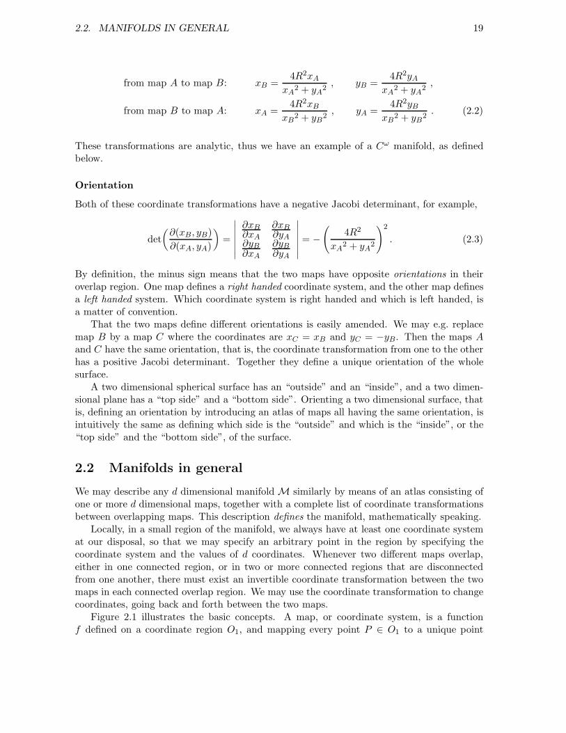
from map A to map B: xB =4R2xA
xA2 + yA
2, yB =
4R2yA
xA2 + yA
2,
from map B to map A: xA =4R2xB
xB2 + yB
2, yA =
4R2yB
xB2 + yB
2. (2.2)
These transformations are analytic, thus we have an example of a Cω manifold, as definedbelow.
Orientation
Both of these coordinate transformations have a negative Jacobi determinant, for example,
det
(∂(xB , yB)
∂(xA, yA)
)=
∣∣∣∣∣∣∣
∂xB∂xA
∂xB∂yA
∂yB∂xA
∂yB∂yA
∣∣∣∣∣∣∣= −
(4R2
xA2 + yA
2
)2
. (2.3)
By definition, the minus sign means that the two maps have opposite orientations in theiroverlap region. One map defines a right handed coordinate system, and the other map definesa left handed system. Which coordinate system is right handed and which is left handed, isa matter of convention.
That the two maps define different orientations is easily amended. We may e.g. replacemap B by a map C where the coordinates are xC = xB and yC = −yB. Then the maps Aand C have the same orientation, that is, the coordinate transformation from one to the otherhas a positive Jacobi determinant. Together they define a unique orientation of the wholesurface.
A two dimensional spherical surface has an “outside” and an “inside”, and a two dimen-sional plane has a “top side” and a “bottom side”. Orienting a two dimensional surface, thatis, defining an orientation by introducing an atlas of maps all having the same orientation, isintuitively the same as defining which side is the “outside” and which is the “inside”, or the“top side” and the “bottom side”, of the surface.
2.2 Manifolds in general
We may describe any d dimensional manifold M similarly by means of an atlas consisting ofone or more d dimensional maps, together with a complete list of coordinate transformationsbetween overlapping maps. This description defines the manifold, mathematically speaking.
Locally, in a small region of the manifold, we always have at least one coordinate systemat our disposal, so that we may specify an arbitrary point in the region by specifying thecoordinate system and the values of d coordinates. Whenever two different maps overlap,either in one connected region, or in two or more connected regions that are disconnectedfrom one another, there must exist an invertible coordinate transformation between the twomaps in each connected overlap region. We may use the coordinate transformation to changecoordinates, going back and forth between the two maps.
Figure 2.1 illustrates the basic concepts. A map, or coordinate system, is a functionf defined on a coordinate region O1, and mapping every point P ∈ O1 to a unique point

20 CHAPTER 2. MANIFOLDS, VECTORS AND TENSORS
x = f(P ) ∈ Rd. By convention, we number the coordinates by means of upper indices,writing
x = (x1, x2, . . . , xd) . (2.4)
Thus, xi = f i(P ) for i = 1, 2, . . . , d, where each f i is a real valued function defined on O1.Since f is a one to one mapping from the region O1 onto its image f(O1), there exists aninverse function f−1 which is a one to one mapping from f(O1) onto O1. The subsets O1 ⊂ Mand f(O1) ⊂ Rd should be open sets, as described below.
x
xf
g
f−1
g−1
O1
O2
f(O1)
g(O2)
PR
d
M
Figure 2.1: A d dimensional manifold M, with two overlapping coordinate systems.
Assume now that P ∈ O1 ∩ O2, where O2 is another coordinate region with anothercoordinate function g. In this second coordinate system the point P has coordinates x =g(P ) ∈ Rd. The relation between the two overlapping coordinate systems is the coordinatetransformation gf−1,
x 7→ x = x(x) = g(P ) = g(f−1(x)) , (2.5)
and the inverse coordinate transformation (gf−1)−1 = fg−1,
x 7→ x = x(x) = f(P ) = f(g−1(x)) . (2.6)
2.2. MANIFOLDS IN GENERAL 21
An atlas with its set of coordinate transformations defines an orientation of the manifoldif all the coordinate transformations have positive Jacobi determinants. If a manifold is notalready oriented, it may nevertheless be orientable, this means that we may make it orientedsimply by switching the orientation of some of the maps. Not all manifolds are orientable,and the simplest counterexample is the Mobius strip. See Problem 1.
Topology
From the mathematical point of view, there are a number of technical points that we do notgo into here in much detail.
For example, it is usually required that the region in the manifold M covered by a mapshould always be an open subset of M. The list of all the open subsets of M is whatmathematicians call the topology of M. One of the defining characteristics of a manifold isthat it has a topology, it is a topological space.
In the most general kind of topological space, only two simple properties are required forthe list of open subsets. First, that the union of a finite or infinite number of open subsetsmust be an open subset, and second, that the intersection of a finite number of open subsetsmust be an open subset. By definition, a closed subset is the complement of an open subset,and hence the intersection of a finite or infinite number of closed subsets is always a closedsubset, whereas the union of a finite number of closed subsets is always a closed subset. Againby definition, the manifold M is both an open and a closed subset of itself, and the emptysubset is both open and closed.
One may ask which subsets of M are both open and closed, in addition to the two trivialcases just mentioned. The answer may be surprising when first encountered, and lies in thefollowing definition. A topological space M is connected if and only if it has no subset whichis both open and closed, apart from the two trivial ones. Any non-trivial subset which issimultaneously open and closed, and which itself has no non-trivial subset with the same twoproperties, is called a connected component of M.
Metric topology
Most topological spaces encountered in physics are metric spaces, in which the topology isdefined in terms of some measure of distances between points. For example, the Euclideanspace Rn, with n = 1, 2, . . ., is a metric space where the distance between two points x =(x1, x2, . . . , xn) and y = (y1, y2, . . . , yn) is the Euclidean distance
s(x, y) = s(y, x) =√
(x1 − y1)2 + (x2 − y2)2 + · · · + (xn − yn)2 . (2.7)
This metric is positive definite and separates points, that is, we have always s(x, y) ≥ 0, ands(x, y) = 0 if and only if x = y. It also satisfies the triangle inequality,
s(x, y) ≤ s(x, z) + s(z, y) (2.8)
for any three points x, y, z. An open subset O of a metric space is defined by the propertythat for any given point x ∈ O there exists a δ > 0 such that y ∈ O whenever s(x, y) < δ.
The Euclidean distance s(x, y) is the length of the shortest curve between x and y, whichis a straight line. And the length of a curve in general is the integral along the curve of theline element ds = s(x, x+ dx). The square of ds is
ds2 = (dx1)2 + (dx2)2 + · · · + (dxn)2 . (2.9)
22 CHAPTER 2. MANIFOLDS, VECTORS AND TENSORS
The standard topology of a d dimensional manifold M is always metric, it is simply thestandard Euclidean topology of Rd, as defined by the Euclidean distance, transferred to themanifold by means of the coordinate mappings. In a manifold M in general we may not havea unique way of measuring distances, such as we have on the surface of the Earth. Fortunately,different measures of distance very often define the same open subsets, and hence it makessense to speak of the topology of a manifold without reference to any particular metric definingthat topology.
Note that the Euclidean line element ds2, Equation (2.9), is positive definit. Both in thespecial and in the general theory of relativity we are going to introduce a physical metricgµν on the four dimensional spacetime. This physical metric is not positive definit in thesame way, and is not directly related to the Euclidean metric on R4 defining the spacetimetopology.
Continuous functions
The concept of continuous functions is meaningful for general topological spaces. The stan-dard “ǫ and δ” definition applies to metric spaces X and Y with metrics sX and sY . It saysthat a function f : X 7→ Y is continuous at a point x ∈ X if for every ǫ > 0 there exists aδ > 0 such that sY (f(x), f(x′)) < ǫ for every x′ ∈ X with sX(x, x′) < δ. If f is continuouseverywhere it is defined, then it is simply said to be continuous.
This definition is easily translated into the more general language of open subsets, andthen amounts to the following. A function f : X 7→ Y , where X and Y are topological spaces,is continuous if and only if the inverse image under f of an open subset O ⊂ Y is always anopen subset of X.
The inverse image of O is denoted by f−1(O), and consists of those points x ∈ X such thatf(x) ∈ O. Note that the notation f−1(O) does not imply that there has to exist a functionf−1 which is inverse to the function f .
Differentiable functions
In the same way as in our mapping of the surface of the Earth, whenever we map an opensubset of M onto an open subset of Rd, we want the mapping to be both continuous anddifferentiable.
The topology on the manifold M defines which functions are continuous, but is not suffi-cient to define what is meant by differentiable functions on M. Lacking any better definition,we simply select some maps and declare them to be continuous and differentiable. A necessaryconsistency condition is then that every time two maps overlap, the coordinate transformationfrom one map to the other must be continuous and differentiable. It is reasonable to imposeeven stronger conditions, for example that every coordinate transformation must belong tothe function class Cn for some n ≥ 2.
By definition, a function from Rk to R, for k = 1, 2, . . ., is of class Cn if all its n-th orderpartial derivatives exist and are continuous everywhere. We also say of a Cn function that itis n times continuously differentiable. The class of continuous functions is called C or C0. Afunction is of class C∞ if all its partial derivatives of all orders exist everywhere.
Analyticity is an even more restrictive condition: an analytic function is not only infinitelydifferentiable everywhere it is defined, but it can be represented by a power series in some

2.3. TENSORS AND TENSOR FIELDS 23
neighbourhood around any given point. The class of analytic functions is called Cω, and it isdifferent from C∞. See Problem 2 for a famous counterexample.
The above definition of the function class Cn (or C∞ or Cω) applies to real valued functionson Rk, i.e. functions Rk 7→ R. But a function f : Rk 7→ Rm is no more nor less than mfunctions from Rk to R, hence we use the obvious terminology and say that f is of class Cn
if all these m functions are of class Cn.
Definition of a manifold
To summarize, we may now define a little bit more precisely what we mean by a d dimensionalmanifold M. It is a topological space, and it is covered by an atlas of one or more coordinatemaps. Each coordinate map, or coordinate system, is a one to one contionuous mappingbetween an open subset of M and an open subset of Rd.
Whenever two maps overlap, there exists an invertible coordinate transformation betweenthem. The coordinate transformation is an invertible transformation between the two openregions of Rd corresponding to the single overlap region in M.
A manifold where all coordinate transformations are of class Cn (or C∞ or Cω) is calleda Cn (or C∞ or Cω) manifold.
2.3 Tensors and tensor fields
One way of writing equations so that they are valid in an arbitrary coordinate system is towrite them as relations between tensors, or between tensor fields. To be concrete we willspeak here about spacetime, which is a four dimensional “space”, but most of what we saymay be generalized directly to the case of a d dimensional manifold. A point in spacetime isgiven by the coordinates
x = xµ = (x0, x1, x2, x3) , (2.10)
where, as a rule, x0 is a time coordinate and the other three are spatial coordinates. We willstick to the usual convention that greek coordinate indices run from 0 til 3. More generally,in a d dimensional space, we would use latin indices running from 1 to d, thus we would write
x = xi = (x1, x2, . . . , xd) . (2.11)
A tensor is a quantity localized at one point in spacetime. Relative to a given coordinatesystem, the tensor has a number of components, and the components transform in certainwell defined ways under coordinate transformations. There are many kinds of tensors, twospecial examples are scalars and vectors. If we have a tensor of a given kind at every point inspacetime, then we have a tensor field. Often we say “tensor” when we actually mean “tensorfield”.
A tensor at a given point is an element of a vector space, and we specify it by specifyinga basis in the vector space, as well as the components of the tensor relative to this basis. Weare free to choose whatever basis we want, but a standard basis is the coordinate basis, whichis uniquely defined by the coordinate system we choose around the point where the tensoris located. The coupling between the tensor basis and the coordinate system means thatthe tensor components get transformed in a particular way when we change our coordinate
24 CHAPTER 2. MANIFOLDS, VECTORS AND TENSORS
system. We will now see in more detail how the components of various types of tensors gettransformed.
A scalar is a trivial tensor, because it has only one component, the value of which isindependent of the coordinate system. A scalar density is slightly less trivial, its singlecomponent gets multiplied by a scale factor when we change coordinate system. We will havesome more to say about densities in Chapter 3.
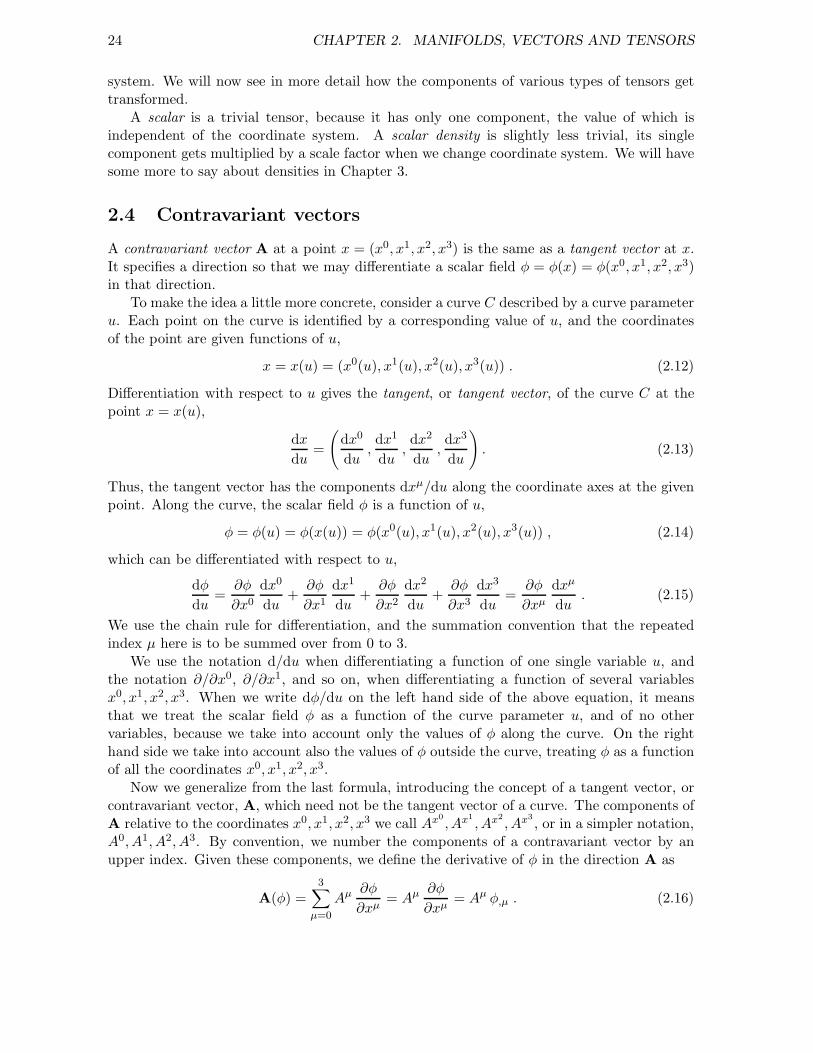
2.4 Contravariant vectors
A contravariant vector A at a point x = (x0, x1, x2, x3) is the same as a tangent vector at x.It specifies a direction so that we may differentiate a scalar field φ = φ(x) = φ(x0, x1, x2, x3)in that direction.
To make the idea a little more concrete, consider a curve C described by a curve parameteru. Each point on the curve is identified by a corresponding value of u, and the coordinatesof the point are given functions of u,
x = x(u) = (x0(u), x1(u), x2(u), x3(u)) . (2.12)
Differentiation with respect to u gives the tangent, or tangent vector, of the curve C at thepoint x = x(u),
dx
du=
(dx0
du,dx1
du,dx2
du,dx3
du
). (2.13)
Thus, the tangent vector has the components dxµ/du along the coordinate axes at the givenpoint. Along the curve, the scalar field φ is a function of u,
φ = φ(u) = φ(x(u)) = φ(x0(u), x1(u), x2(u), x3(u)) , (2.14)
which can be differentiated with respect to u,
dφ
du=
∂φ
∂x0
dx0
du+
∂φ
∂x1
dx1
du+
∂φ
∂x2
dx2
du+
∂φ
∂x3
dx3
du=
∂φ
∂xµ
dxµ
du. (2.15)
We use the chain rule for differentiation, and the summation convention that the repeatedindex µ here is to be summed over from 0 to 3.
We use the notation d/du when differentiating a function of one single variable u, andthe notation ∂/∂x0, ∂/∂x1, and so on, when differentiating a function of several variablesx0, x1, x2, x3. When we write dφ/du on the left hand side of the above equation, it meansthat we treat the scalar field φ as a function of the curve parameter u, and of no othervariables, because we take into account only the values of φ along the curve. On the righthand side we take into account also the values of φ outside the curve, treating φ as a functionof all the coordinates x0, x1, x2, x3.
Now we generalize from the last formula, introducing the concept of a tangent vector, orcontravariant vector, A, which need not be the tangent vector of a curve. The components ofA relative to the coordinates x0, x1, x2, x3 we call Ax0
, Ax1, Ax2
, Ax3, or in a simpler notation,
A0, A1, A2, A3. By convention, we number the components of a contravariant vector by anupper index. Given these components, we define the derivative of φ in the direction A as
A(φ) =3∑
µ=0
Aµ ∂φ
∂xµ= Aµ ∂φ
∂xµ= Aµ φ,µ . (2.16)
2.4. CONTRAVARIANT VECTORS 25
We use again the summation convention for the repeated index µ, and we introduce a shorternotation for the partial derivative,
φ,µ =∂φ
∂xµ. (2.17)
Note that the component Aν is the derivative of the coordinate xν in the direction A,
A(xν) = Aµ ∂xν
∂xµ= Aµ δν
µ = Aν . (2.18)
We may write
A = Aµ ∂
∂xµ= Aµ eµ , (2.19)
expanding in the special basis vectors defined by the coordinate system,
eµ =∂
∂xµ. (2.20)
Instead of this coordinate basis for the space of contravariant vectors we could have chosen amore general basis
eA = eµA eµ = eµA∂
∂xµ, A = 0, 1, 2, 3 , (2.21)
where the 4 × 4 = 16 coefficients eµA would be functions of x = (x0, x1, x2, x3). However, wewill stick to the coordinate basis, at least in the present chapter.
Equation (2.16) determines how the components of the vector get transformed when wechange to a different set of coordinates x = (x0, x1, x2, x3). The chain rule for differentiationgives the following transformation formula for the differentiation operators,
∂
∂xµ=∂xκ
∂xµ
∂
∂xκ. (2.22)
Since the formula is completely general, we may interchange x and x to get that
∂
∂xµ=∂xκ
∂xµ
∂
∂xκ. (2.23)
The 4× 4 matrix ∂x/∂x is sometimes called the Jacobi matrix of the coordinate transforma-tion, its determinant is the Jacobi determinant entering in the formula for changing variablesin a multiple integral. The two matrices ∂x/∂x and ∂x/∂x are inverses of each other, a resultwhich also follows directly from the chain rule,
δµν =
∂xµ
∂xν=∂xκ
∂xν
∂xµ
∂xκ=∂xµ
∂xν=∂xκ
∂xν
∂xµ
∂xκ. (2.24)
Figure 2.2 illustrates the relation between the partial derivatives in two different coordinatesystems in the plane. For example, ∂/∂x1 is a tangent vector of the curve x2 = constant,pointing in the direction in which x1 increases.
Since the tangent vector A is the same, no matter which basis we expand it in, itscomponents must get transformed so that
A = Aµ ∂
∂xµ= Aµ ∂
∂xµ. (2.25)
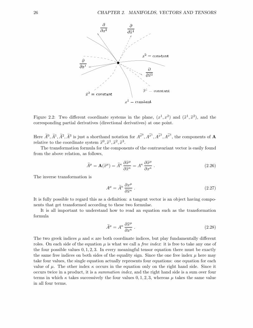
26 CHAPTER 2. MANIFOLDS, VECTORS AND TENSORSex1x1
x2ex2x2 = onstant
ex1 = onstantex2 = onstant x1 = onstantFigure 2.2: Two different coordinate systems in the plane, (x1, x2) and (x1, x2), and thecorresponding partial derivatives (directional derivatives) at one point.
Here A0, A1, A2, A3 is just a shorthand notation for Ax0, Ax1
, Ax2, Ax3
, the components of Arelative to the coordinate system x0, x1, x2, x3.
The transformation formula for the components of the contravariant vector is easily foundfrom the above relation, as follows,
Aµ = A(xµ) = Aκ ∂xµ
∂xκ= Aκ ∂x
µ
∂xκ. (2.26)
The inverse transformation is
Aµ = Aκ ∂xµ
∂xκ. (2.27)
It is fully possible to regard this as a definition: a tangent vector is an object having compo-nents that get transformed according to these two formulae.
It is all important to understand how to read an equation such as the transformationformula
Aµ = Aκ ∂xµ
∂xκ. (2.28)
The two greek indices µ and κ are both coordinate indices, but play fundamentally differentroles. On each side of the equation µ is what we call a free index: it is free to take any one ofthe four possible values 0, 1, 2, 3. In every meaningful tensor equation there must be exactlythe same free indices on both sides of the equality sign. Since the one free index µ here maytake four values, the single equation actually represents four equations: one equation for eachvalue of µ. The other index κ occurs in the equation only on the right hand side. Since itoccurs twice in a product, it is a summation index, and the right hand side is a sum over fourterms in which κ takes successively the four values 0, 1, 2, 3, whereas µ takes the same valuein all four terms.
2.4. CONTRAVARIANT VECTORS 27
There is an easy way to remember the transformation formula from “old” coordinates xto “new” coordinates x, Equation (2.28). Just observe that there is one index, κ, referring tothe “old” coordinates, and one index, µ, referring to the “new” coordinates.
From contravariant vectors we generalize to contravariant tensors. That A is a contravari-ant tensor of rank two means that it can be written as
A = Aµν eµ ⊗ eν , (2.29)
where eµ ⊗ eν is the tensor product of the basis vectors. This definition is circular, strictlyspeaking, since we have not defined the tensor product in an independent way. The impor-tant point is that the components Aµν have two upper indices, and as long as we stick tothe coordinate basis vectors, Equation (2.20), the following transformation formula is to beapplied when we change our coordinate system,
Aµν =∂xµ
∂xκ
∂xν
∂xλAκλ . (2.30)
Each of the two indices gets transformed as a contravariant vector index. This transformationproperty of the tensor components may be taken as the definition of a contravariant tensorof rank two.
It should be obvious how to generalize further to tensors with any number of contravari-ant indices. Each contravariant index gets transformed under a coordinate transformationxµ 7→ xµ by means of the matrix ∂xµ/∂xν , consisting of all partial derivatives of the “new”coordinates with respct to the “old” ones.
Take as an example the connection between the Cartesian coordinates x, y in the plane andthe polar coordinates r, ϕ, as given in the Equations (1.72), (1.79) and (1.80). Equation (2.26)gives for a contravariant vector A that
Ar =∂r
∂xAx +
∂r
∂yAy = cosϕAx + sinϕAy ,
Aϕ =∂ϕ
∂xAx +
∂ϕ
∂yAy = −sinϕ
rAx +
cosϕ
rAy . (2.31)
Equation (2.30) gives for a contravariant tensor of rank two that, e.g.,
Arϕ =∂r
∂x
∂ϕ
∂xAxx +
∂r
∂y
∂ϕ
∂xAyx +
∂r
∂x
∂ϕ
∂yAxy +
∂r
∂y
∂ϕ
∂yAyy
=cosϕ sinϕ
r(−Axx +Ayy) − sin2ϕ
rAyx +
cos2ϕ
rAxy . (2.32)
Commutation of contravariant vector fields
A vector field A acting on a scalar field φ gives a new scalar field A(φ), by Equation (2.16).Hence, given two vector fields
A = Aµ ∂
∂xµ, B = Bν ∂
∂xν, (2.33)
we may act on the scalar field φ with both of them in succession. For example, acting withB first and with A afterwards gives the following result,
A(B(φ)) = Aµ ∂
∂xµ
(Bν ∂φ
∂xν
)= Aµ ∂B
ν
∂xµ
∂φ
∂xν+AµBν ∂2φ
∂xµ∂xν. (2.34)
28 CHAPTER 2. MANIFOLDS, VECTORS AND TENSORS
By definition, the operator product AB is the operator mapping φ into A(B(φ)). It is not avector field, because it involves second order derivatives of φ.
The partial derivative operators ∂/∂xµ and ∂/∂xν commute, and therefore we have that
AµBν ∂2φ
∂xµ∂xν= AµBν ∂2φ
∂xν∂xµ= AνBµ ∂2φ
∂xµ∂xν. (2.35)
The last equality sign is obtained by the frequently used trick of renaming the summationindices µ and ν: the value of a sum never depends on the name of a summation index. Thisrelation implies that the second derivative terms cancel in the commutator between A andB, which is the operator C = [A,B] = AB −BA, explicitly defined by the relation
C(φ) = A(B(φ)) − B(A(φ)) =
(Aµ ∂B
ν
∂xµ−Bµ ∂A
ν
∂xµ
)∂φ
∂xν. (2.36)
Thus, C is a vector field with the components
Cν = Aµ ∂Bν
∂xµ−Bµ ∂A
ν
∂xµ. (2.37)
It follows directly from the definition that the commutator is antisymmetric,
[B,A] = −[A,B] . (2.38)
The Jacobi identity
[A, [B,C]] + [B, [C,A]] + [C, [A,B]] = 0 (2.39)
follows directly from the definition [A,B] = AB − BA, together with the associative lawA(BC) = (AB)C.
2.5 Covariant vectors, mixed tensors, and contraction
A covariant vector is the same as a 1-form,
B = Bµ eµ = Bµ dxµ , (2.40)
where we have used the coordinate basis vectors
eµ = dxµ . (2.41)
The components of B we call Bxµ , or more simply Bµ, with a lower index.The 1-form B is an object which can be integrated along the curve C defined by Equa-
tion (2.12). If the curve parameter u ranges from u1 to u2, then the integral is
∫
CB =
∫
CBµ dxµ =
∫ u2
u1
du Bµ(x(u))dxµ(u)
du. (2.42)
The derivatives dxµ/du in the integral are the components of the tangent vector of the curve,as in Equation (2.13).
The covariant vector B is the same if we choose a different coordinate system, hence
B = Bµ dxµ = Bµ dxµ , (2.43)
2.5. COVARIANT VECTORS, MIXED TENSORS, AND CONTRACTION 29
and this determines the transformation formula for the components. Since
dxκ =∂xκ
∂xµdxµ , (2.44)
by the chain rule, we must have that
Bµ =∂xκ
∂xµBκ . (2.45)
Again, Bµ is a simpler notation for Bxµ.
If B is a covariant tensor of rank two, this means that it can be written as
B = Bµν eµ ⊗ eν = Bµν dxµ ⊗ dxν , (2.46)
where eµ⊗eν = dxµ⊗dxν is the tensor product of the basis vectors. The components Bµν arewritten with two lower indices, each of which gets transformed in the same way as a covariantvector index,
Bµν =∂xκ
∂xµ
∂xλ
∂xνBκλ . (2.47)
Again it should be obvious how to generalize to tensors with an arbitrary number of co-variant indices, and further to tensors with an arbitrary combination of contravariant andcovariant indices. A tensor of rank n has n indices, whether they are contravariant or covari-ant. If we want to be a little more precise, we may say that a tensor has rank (m,n) if it hasm contravariant and n covariant indices.
For a tensor Aµν with one contravariant and one covariant index the following transforma-
tion formula holds,
Aµν =
∂xµ
∂xκ
∂xλ
∂xνAκ
λ . (2.48)
We may contract the upper and the lower index, that is, we put them equal and sum over allpossible values. The result of this operation is independent of the coordinate system, in factwe have that
Aµµ =
∂xµ
∂xκ
∂xλ
∂xµAκ
λ = δλκA
κλ = Aκ
κ . (2.49)
The result of the contraction is a scalar, i.e. a quantity which is independent of the coordinatesystem. If we regard Aµ
ν as a matrix, then Aµµ is the sum of the diagonal matrix elements, the
trace of the matrix.We may always perform such a contraction between an upper and a lower index, no
matter how many other indices a tensor has. The contraction produces a new tensor havingone upper and one lower index less than the uncontracted tensor. We produce a tensor ofrank (m−1, n−1) from a tensor of rank (m,n). Tensor product and contraction are oppositeoperations in the sense that one increases and the other one decreases the number of indices.
Let us elaborate on our favourite example, the connection between Cartesian coordinatesx, y and polar coordinates r, ϕ in the plane, as given in the Equations (1.72), (1.79) and (1.80).Equation (2.45) gives for a covariant vector B that
Br =∂x
∂rBx +
∂y
∂rBy = cosϕBx + sinϕBy ,
Bϕ =∂x
∂ϕBx +
∂y
∂ϕBy = −r sinϕBx + r cosϕBy . (2.50)
30 CHAPTER 2. MANIFOLDS, VECTORS AND TENSORS
For a mixed contravariant and covariant tensor of rank 2, i.e. rank (1, 1), we get for thediagonal elements that
Arr =
∂r
∂x
∂x
∂rAx
x +∂r
∂y
∂x
∂rAy
x +∂r
∂x
∂y
∂rAx
y +∂r
∂y
∂y
∂rAy
y
= cos2ϕAxx + cosϕ sinϕ (Ay
x +Axy) + sin2ϕAy
y ,
Aϕϕ =
∂ϕ
∂x
∂x
∂ϕAx
x +∂ϕ
∂y
∂x
∂ϕAy
x +∂ϕ
∂x
∂y
∂ϕAx
y +∂ϕ
∂y
∂y
∂ϕAy
y (2.51)
= sin2ϕAxx − cosϕ sinϕ (Ay
x +Axy) + cos2ϕAy
y .
This shows explicitly that contraction gives the same result in Cartesian and polar coordinates,
Arr +Aϕ
ϕ = Axx +Ay
y . (2.52)
2.6 Symmetry and antisymmetry of tensors
An important consequence of the transformation formula in Equation (2.30) is that if acontravariant tensor of rank two has either symmetric or antisymmetric components in onecoordinate system, that is, if
Aµν = ǫAνµ , (2.53)
with ǫ = 1 or ǫ = −1, then it has components with the same symmetry in any coordinatesystem,
Aµν =∂xµ
∂xκ
∂xν
∂xλAκλ = ǫ
∂xµ
∂xκ
∂xν
∂xλAλκ = ǫAνµ . (2.54)
Thus, the property of such a tensor that it has symmetric components (ǫ = +1), or antisym-metric components (ǫ = −1), is independent of the coordinate system, it is a property of thetensor itself. This observation is quite generally valid, for contravariant or covariant tensors,for tensors with any number of indices, and for general symmetry classes.
Totally symmetric and totally antisymmetric tensors of arbitrary rank are of particularinterest. A contravariant tensor, as an example, is symmetric, or totally symmetric, if theorder of the indices is irrelevant for the value of a component Aµν...ρ. It is antisymmetric, ortotally antisymmetric, if the order of the indices is relevant only for the sign of the componentAµν...ρ, so that the sign changes for every interchange of two indices. A couple of examplesshould illustrate the concepts.
An arbitrary contravariant tensor of rank two, Aµν , may be written as a sum
Aµν = A(µν) +A[µν] (2.55)
of a symmetric part
A(µν) =1
2(Aµν +Aνµ) (2.56)

2.7. THE METRIC TENSOR 31
and an antisymmetric part
A[µν] =1
2(Aµν −Aνµ) . (2.57)
This splitting is unique and, as already stated, invariant under coordinate transformations.A contravariant tensor of rank three, Aλµν , has one totally symmetric part,
A(λµν) =1
6(Aλµν +Aνλµ +Aµνλ +Aµλν +Aλνµ +Aνµλ) , (2.58)
one totally antisymmetric part,
A[λµν] =1
6(Aλµν +Aνλµ +Aµνλ −Aµλν −Aλνµ −Aνµλ) , (2.59)
and in addition a third part of mixed symmetry,
Aλµν −A(λµν) −A[λµν] =1
3(2Aλµν −Aνλµ −Aµνλ) . (2.60)
This splitting into different symmetry components is still invariant under coordinate trans-formations.
In the same way, we may split covariant tensors with two or three indices into symmetrycomponents. Tensors with more than three indices, contravariant or covariant, may also besplit into symmetry components, but the number of different components increases rapidlywith the number of indices. Partial symmetrization or antisymmetrization is possible, wemay define for example
Aλ[µν] =1
2(Aλµν −Aλνµ) . (2.61)
Contraction, symmetry and antisymmetry
One result which is trivial enough, but is used so often that it merits special attention, isthat contraction of two symmetric indices against two antisymmetric indices must always givezero. For example, AµνBµν = 0 if Aµν = Aνµ and Bµν = −Bνµ. The proof is as follows,
AµνBµν = AνµBµν = −AνµBνµ = −AµνBµν . (2.62)
The last equality follows from the fact that µ and ν are summation indices, so that we arefree to rename them as we like, for example to interchange their names. When AµνBµν =−AµνBµν , it means that AµνBµν = 0.
2.7 The metric tensor
The Kronecker symbol with one upper and one lower index,
δµν =
1 when µ = ν,0 when µ 6= ν,
(2.63)
32 CHAPTER 2. MANIFOLDS, VECTORS AND TENSORS
actually defines a tensor. In fact, if we define Aµν to be a tensor with components Aµ
ν = δµν in
one coordinate system, then when we transform to another coordinate system the transformedcomponents are
Aµν =
∂xµ
∂xκ
∂xλ
∂xνAκ
λ =∂xµ
∂xκ
∂xλ
∂xνδκλ =
∂xµ
∂xκ
∂xκ
∂xν= δµ
ν . (2.64)
This is a rather special tensor: it is invariant in the sense that it has the same componentsδµν in any coordinate system.
The metric tensor gµν , the metric for short, is used for lowering indices. It is a covarianttensor of rank two. For example, we convert a contravariant vector Aµ into a covariant vectorAµ, which we call by the same name A, by defining
Aµ = gµκAκ . (2.65)
We define the scalar product between two contravariant vectors A and B as
A · B = AµBµ = gµνAµBν . (2.66)
Thus, the metric tensor enables us to contract two upper indices against each other. Thescalar product A · B is a scalar, as the name says. If the scalar product of a vector A withitself, A2 = A · A, is non-negative, then we may define the length of A as
|A| =√
A2 . (2.67)
If A2 > 0 and B2 > 0, then we may define the angle θ between the vectors A and B by therelation
A ·B = |A| |B| cos θ . (2.68)
We assume that the matrix gµν is always non-singular, i.e. invertible. The inverse matrixwe write as gµν , and we use it for raising indices,
Aµ = gµκAκ . (2.69)
That gµν and gµν are each others inverses, means that
gµκgκν = gνκgκµ = δµ
ν . (2.70)
This definition is independent of the coordinate system, since contraction is a coordinateindependent operation, and since the Kronecker tensor δµ
ν has the same components in allcoordinate systems. By definition, the result of raising one index of the metrix tensor is δµ
ν ,thus the Kronecker tensor is simply the metric tensor with one upper and one lower index.
We will always assume here that the metric tensor is symmetric, i.e. that gµν = gνµ. Itfollows that gµν = gνµ, since the inverse of a symmetric matrix is symmetric.
The symmetry has another less obvious consequence. By a suitable coordinate transfor-mation,
gµν =∂xκ
∂xµ
∂xλ
∂xνgκλ , (2.71)
2.7. THE METRIC TENSOR 33
we may always diagonalize the metric at one arbitrary isolated point, that is, we may obtainthat gµν = 0 for µ 6= ν, at this one point. The number of positive and negative diagonalelements of the metric in such a coordinate system is a characteristic property which is calledthe signature of the metric. The metric in spacetime has everywhere signature (1, 3), thatis, when diagonalized it has always one positive diagonal element, corresponding to the timedirection, and three negative diagonal elements, corresponding to the spatial directions. Theoverall sign has no very deep significance, so that a metric of signature (3, 1) may serve justas well as a metric of signature (1, 3). In fact, these opposite sign conventions are both incommon use, but we have to fix a convention and we decide on the (1, 3) convention.
An important quantity is the determinant of the metric tensor,
g = det(gµν) . (2.72)
It may be positive or negative, dependent on the signature of the metric, and for the signature(1, 3) we have g < 0.
Variation of the metric
An infinitesimal variation ∆gµν of gµν will lead to infinitesimal variations ∆gµν of gµν and∆g of g. The definition of gµν , Equation (2.70), gives immediately that
∆gµκgκλ + gµκ∆gκλ = 0 . (2.73)
Multiplying with gνλ and using the relation gνλgκλ = δνκ, we deduce that
∆gµν = −gµκgνλ∆gκλ . (2.74)
The relation between ∆g and ∆gµν is slightly more involved. In order to derive it we mayuse the connection between the determinant and the Levi–Civita symbol, Equation (1.5). Infour dimensions we have that
gακ gβλ gγµ gδν ǫκλµν = g ǫαβγδ . (2.75)
The Levi–Civita symbol with upper or lower indices, ǫκλµν or ǫκλµν , is totally antisymmetric,and ǫ0123 = ǫ0123 = 1. The convention that the metric tensor is used for lowering and raisingindices does not hold for the Levi–Civita symbol, as we define it here. The above relationmeans e.g. that
gβλ gγµ gδν ǫκλµν = g gκρ ǫρβγδ . (2.76)
By varying gµν , we get for example that
∆g ǫαβγδ = (∆gακ gβλ gγµ gδν + gακ ∆gβλ gγµ gδν
+gακ gβλ ∆gγµ gδν + gακ gβλ gγµ ∆gδν) ǫκλµν
= ∆gακ gκρ g ǫρβγδ + ∆gβλ g
λρ g ǫαργδ (2.77)
+∆gγµ gµρ g ǫαβρδ + ∆gδν g
νρ g ǫαβγρ .
We multiply this equation by ǫαβγδ and use that, e.g.,
ǫαβγδǫρβγδ = 6δαρ , ǫαβγδǫαβγδ = 24 . (2.78)
34 CHAPTER 2. MANIFOLDS, VECTORS AND TENSORS
Then we arrive at the following relation, which can be proved by similar methods in anarbitrary dimension,
∆g = g gνµ ∆gµν = −g gνµ ∆gµν . (2.79)
Rewriting this formula in the form
gνµ =1
g
∂g
∂gµν, (2.80)
we may recognize it as Kramer’s rule for inverting a matrix. Here we differentiate with respectto one component, say g01, as if g01 and g10 were independent, in spite of the symmetrycondition gµν = gνµ.
Later on, we will need a formula for the variation of√|g|, which is
∆√|g| =
1
2√|g|
|g|g
∆g =1
2
√|g| gνµ ∆gµν = −1
2
√|g| gνµ ∆gµν . (2.81)
The special theory of relativity
In the special theory of relativity we normally choose time and space coordinates such thatthe metric gets the simple form
gµν = ηµν =
1 0 0 00 −1 0 00 0 −1 00 0 0 −1
, (2.82)
first introduced by Minkowski in 1908, although with the opposite sign. Then we have
gµν = ηµν =
1 0 0 00 −1 0 00 0 −1 00 0 0 −1
. (2.83)
It is not always possible to choose the coordinate system so that the metric gets this simpleform. The necessary and sufficient condition is that the curvature tensor defined by themetric vanishes, and of course that the signature is (1, 3). See the Chapters 5 and 6. Thus,the specialty of the special theory of relativity is the assumption that spacetime is flat.
2.7. THE METRIC TENSOR 35
Problems
1. A Mobius strip is made e.g. from a rectangle in the (x, y) plane with its corners at (0, 0),(5, 0), (0, 1) and (5, 1). We glue the two edges x = 0 and x = 5 against each other, withthe two opposite corners (0, 0) and (5, 1) together, and the corners (0, 1) and (5, 0) alsotogether.Prove that the Mobius strip is not orientable.
2. Define f(0) = 0, and
f(x) = e−1
x2 for x 6= 0 .
Show that this function f : R 7→ R is C∞ (infinitely differentiable) everywhere.Find its Taylor series expansion about x = 0.Is it Cω (analytic) at x = 0? At x 6= 0?
3. Express the Euclidean metric ds2 = dx2+dy2 in the (x, y) plane in the polar coordinates(r, ϕ). By definition, r ∈ [0,∞〉, ϕ ∈ [0, 2π], and x = r cosϕ, y = r sinϕ.
4. Express the three dimensional Euclidean metric ds2 = dx2 + dy2 + dz2 in the polarcoordinates (r, θ, ϕ), defined by the relations r ∈ [0,∞〉, θ ∈ [0, π], ϕ ∈ [0, 2π], and
x = r sin θ cosϕ , y = r sin θ sinϕ , z = r cos θ .
Compare with Equation (1.15).
5. Put r = a = constant in Problem 4. This defines the surface of a sphere of radius a,such that a point on the surface is given by the polar coordinates (θ, ϕ).Write in polar coordinates the metric ds2 = dx2+dy2+dz2 on the surface of the sphere.

36 CHAPTER 2. MANIFOLDS, VECTORS AND TENSORS
Chapter 3
Tensor algebra
3.1 Tensor product
As an example, let A be a contravariant vector with components Aµ and B a covariant vectorwith components Bν . Then the tensor product of A and B is a tensor C = A ⊗ B havingthe components
Cµν = AµBν . (3.1)
If A and B are tensor fields, then C = A⊗B is a tensor field. The tensor product of fields isa pointwise product: the value of the field C = A⊗B at the point x is C(x) = A(x)⊗B(x).
The tensor product is identical to the usual product in the special case where at leastone of the factors is a scalar, or a scalar field. In general, the tensor product of two tensorsof ranks m and n is a tensor of rank m + n. The fact that the tensor product is usually atensor of higher rank than each of the factors, distinguishes it from other types of product,such as multiplication of numbers or matrices, scalar product between vectors, or the threedimensional vector product.
The tensor product is non-commutative,
A ⊗B 6= B ⊗ A when A 6= B , (3.2)
except when one of the factors is a scalar. In the above example, the tensor product C = A⊗Bof a contravariant vector A and a covariant vector B, the components of D = B⊗ A are
Dνµ = BνA
µ = Cµν . (3.3)
As another example, the tensor products C = A ⊗ B and D = B ⊗ A of two contravariantvectors A 6= B are also different, because
Cµν = AµBν = Dνµ 6= Dµν . (3.4)
The tensor product is assosiative,
(A⊗ B) ⊗ C = A⊗ (B ⊗ C) , (3.5)
and therefore we write A ⊗ B ⊗ C without parentheses. It is bilinear: when a and b arescalars, then
A⊗ (aB + bC) = aA⊗ B + bA⊗ C ,
(aA + bB) ⊗ C = aA⊗ C + bB ⊗C . (3.6)
37
38 CHAPTER 3. TENSOR ALGEBRA
3.2 Forms and exterior product
Antisymmetric covariant tensors play a major role in the theory of differentiation and inte-gration. Therefore they have got a formalism of their own with its own terminology. Anantisymmetric covariant tensor of rank n is called an n-form. In particular, a 0-form is thesame as a scalar, and a 1-form is the same as a covariant vector.
The simplest example where the antisymmetry enters is a 2-form A. Using the coordinatebasis, Equation (2.41), and exploiting the antisymmetry we get that
A = Aµν dxµ ⊗ dxν = Aµν1
2(dxµ ⊗ dxν − dxν ⊗ dxµ) . (3.7)
At this point it is natural to introduce the antisymmetric tensor product “∧” (“wedge”), alsocalled the exterior product. For two basis vectors eµ = dxµ and eν = dxν we define
dxµ ∧ dxν = dxµ ⊗ dxν − dxν ⊗ dxµ . (3.8)
This definition gives that
A =1
2Aµν dxµ ∧ dxν =
∑
µ<ν
Aµν dxµ ∧ dxν . (3.9)
In the first sum here we sum freely over all µ and ν, but since Aµν = −Aνµ and dxµ ∧ dxν =−dxν ∧ dxµ, two and two terms in the sum are equal. The factor of 1/2 compensates for thedouble counting. In the last sum we sum over terms that are all independent, thus avoidingthe extra factor of 1/2. The following notation is sometimes used,
A =∑
µ<ν
Aµν dxµ ∧ dxν = A|µν| dxµ ∧ dxν , (3.10)
with the absolute value sign in |µν| meaning that µ < ν. The explicit sum is
A = A01 dx0 ∧ dx1 +A02 dx0 ∧ dx2 +A03 dx0 ∧ dx3
+A12 dx1 ∧ dx2 +A13 dx1 ∧ dx3 +A23 dx2 ∧ dx3 . (3.11)
For three basis vectors we define
dxλ ∧ dxµ ∧ dxν = dxλ ⊗ dxµ ⊗ dxν + dxν ⊗ dxλ ⊗ dxµ + dxµ ⊗ dxν ⊗ dxλ
−dxµ ⊗ dxλ ⊗ dxν − dxλ ⊗ dxν ⊗ dxµ − dxν ⊗ dxµ ⊗ dxλ . (3.12)
And so on. The exterior product dxλ ∧ dxµ ∧ . . . ∧ dxρ of n arbitrary basis vectors is bydefinition antisymmetric under an interchange of any two indices, hence it is zero if twoindices are equal. The antisymmetry may be used in order to interchange the indices, e.g. sothat they always come in an increasing order, λ < µ < . . . < ρ.
Unfortunately (but not surprisingly!) two different normalization conventions exist forthe exterior product. The alternative convention prescribes an extra factor of 1/n! in thedefinition of the exterior product of n basis vectors. Whatever convention is adopted, factorslike n or n! must turn up somewhere.
In general we define the exterior product of an m-form
A =1
m!Aαβ...η dxα ∧ dxβ ∧ . . . ∧ dxη (3.13)
3.2. FORMS AND EXTERIOR PRODUCT 39
and an n-form
B =1
n!Bµν...ρ dxµ ∧ dxν ∧ . . . ∧ dxρ (3.14)
as
A ∧ B =1
m!n!Aαβ...η Bµν...ρ dxα ∧ dxβ ∧ . . . ∧ dxη ∧ dxµ ∧ dxν ∧ . . . ∧ dxρ . (3.15)
Thus, C = A ∧B is an (m+ n)-form,
C =1
(m+ n)!Cαβ...ηµν...ρ dxα ∧ dxβ ∧ . . . ∧ dxη ∧ dxµ ∧ dxν ∧ . . . ∧ dxρ , (3.16)
with components
Cαβ...ηµν...ρ =(m+ n)!
m!n!A[αβ...η Bµν...ρ] . (3.17)
The square parentheses “[ ]” imply an antisymmetrization over all of the m+ n indices.The exterior product is associative: for an arbitrary m-form A, n-form B and p-form C
we have that
(A ∧B) ∧ C = A ∧ (B ∧ C) , (3.18)
and therefore we write A ∧ B ∧C without parentheses. Note that
A ∧ B = (−1)mn B ∧ A . (3.19)
The exterior product is antisymmetric if both factors are of odd rank, otherwise it is sym-metric, i.e. commutative.
Let us take as example three dimensional space with Euclidean coordinates (x, y, z). Theexterior product of two 1-forms
A = Axdx+Aydy +Azdz , B = Bxdx+Bydy +Bzdz , (3.20)
is a 2-form
A ∧ B = (AyBz −AzBy) dy ∧ dz + (AzBx −AxBz) dz ∧ dx
+(AxBy −AyBx) dx ∧ dy . (3.21)
In three dimensions there exist three linearly independent 1-forms, and just as many linearlyindependent 2-forms. It is therefore possible to define a duality between 1-forms and 2-forms,e.g. by postulating that
dx↔ dy ∧ dz , dy ↔ dz ∧ dx , dz ↔ dx ∧ dy . (3.22)
In this way, the exterior product becomes identical to the well known vector product,
A ∧ B ↔ A × B . (3.23)
40 CHAPTER 3. TENSOR ALGEBRA
The exterior product between three 1-forms corresponds to the triple product between vectors,
A ∧ B ∧ C = ((AyBz −AzBy)Cx + (AzBx −AxBz)Cy
+(AxBy −AyBx)Cz) dx ∧ dy ∧ dz (3.24)
↔ (A × B) · C = A · (B × C) .
At this point a warning may be useful. The exterior product A∧B∧C of three covariantvectors in three dimensions is not a vector, it is a 3-form, which is the dual of a scalar.Thus, it is fundamentally different from either of the two vector products (A × B) × C andA× (B ×C), which are both vectors. Unlike most products we are familiar with, the vectorproduct is not associative, in general we have (A × B) × C 6= A × (B × C).
As we will see later on, it is possible to define quite generally a duality between n-formsand (d − n)-forms in d dimensions, for arbitrary d and n, as soon as we have given a metrictensor. The present example with d = 3 and n = 1 (or n = 2) is just a special case.
Symmetric tensor product
We might want to define a symmetric tensor product similar to the antisymmetric product,writing for example
dxµ ∨ dxν = dxµ ⊗ dxν + dxν ⊗ dxµ . (3.25)
The factors in the symmetric tensor product must be tensors of the same rank, and the rank ofthe product is twice the rank of each factor. In other respects, the symmetric tensor productis much like ordinary multiplication, since it is both associative and commutative.
For example, when we define the metric tensor gµν by writing the line element
ds2 = gµν dxµ dxν , (3.26)
we might interpret this as an expansion of the covariant tensor g, of rank two, in terms ofthe basis dxµ ⊗ dxν in the space of all rank two covariant tensors,
g = gµν dxµ ⊗ dxν =1
2gµν (dxµ ⊗ dxν + dxν ⊗ dxµ) . (3.27)
The last equality follows because the metric is symmetric, gµν = gνµ. We will make no use ofthe symmetric tensor product here.
3.3 Tensor densities
We say that a quantity T κλ , for example, is a tensor density, as opposed to a tensor, if it is
subject to the following transformation formula,
T κλ =
∣∣∣∣det
(∂x
∂x
)∣∣∣∣∂xκ
∂xα
∂xβ
∂xλTα
β , (3.28)
containing the absolute value of the Jacobi determinant for the inverse coordinate transfor-mation. Scalar densities are important in field theory, because a sufficient condition for theinvariance of a theory under general coordinate transformations is that the Lagrange densitytransforms as a scalar density.

3.3. TENSOR DENSITIES 41
More generally, we may have tensor densities with an arbitrary number of contravariantand covariant indices, and of arbitrary weight ν, meaning that the transformation involvesthe ν-th power of the absolute value of the Jacobi determinant. The most important classof tensor densities are the antisymmetric contravariant densities of weight 1, which we callsimply densities. A density of rank n, having n antisymmetric contravariant indices, may becalled an n-density.
A tensor density of weight 0 is the same as a tensor. The difference between tensors andtensor densities is of course invisible if we restrict ourselves to volume preserving coordinatetransformations, which have determinants of ±1. Examples are space and time translationsand Lorentz transformations.
A pseudo tensor density transforms exactly like a tensor density under a coordinate trans-formation with a positive Jacobi determinant, but with the opposite sign when the Jacobideterminant is negative. Thus, the above formula would be modified as follows,
T κλ = det
(∂x
∂x
)∂xκ
∂xα
∂xβ
∂xλTα
β . (3.29)
The distinction between tensor densities and pseudo tensor densities is often not essential,and sometimes we refer to both of them as tensor densities.
The prototype of a scalar density is√|g|, since
√|g| =
√|det(gµν)| =
√∣∣∣∣det
(∂xρ
∂xµgρσ
∂xσ
∂xν
)∣∣∣∣ =∣∣∣∣det
(∂x
∂x
)∣∣∣∣√|g| . (3.30)
This proves, by the way, that√|detAµν | is a scalar density whenever Aµν is a covariant
tensor of rank two.The product of a tensor density and a tensor is again a tensor density. For example, if Aκ
λ
is a tensor, then T κλ =
√|g|Aκ
λ is a tensor density.The prototype of a pseudo density, in contrast to a density, is the Levi–Civita symbol with
upper indices, ǫκλ...ρ, i.e. ǫκλµν in the four dimensional case. In fact, if we define a quantityT κλµν having the components
T κλµν = ǫκλµν (3.31)
in every coordinate system, then the transformation formula
T κλµν = det
(∂x
∂x
)∂xκ
∂xα
∂xλ
∂xβ
∂xµ
∂xγ
∂xν
∂xδTαβγδ (3.32)
holds, because
∂xκ
∂xα
∂xλ
∂xβ
∂xµ
∂xγ
∂xν
∂xδǫαβγδ = det
(∂x
∂x
)ǫκλµν =
(det
(∂x
∂x
))−1
ǫκλµν . (3.33)
Thus, if we multiply a tensor by ǫκλµν , and maybe contract one or more upper indicesagainst the same number of lower indices, the result will be a (pseudo) tensor density.
Note that the scalar density√|g| simply gives the “size” of the tensor density ǫκλµν , as
measured by the metric tensor. In fact, we have that
gακ gβλ gγµ gδν ǫαβγδ ǫκλµν = 24g . (3.34)

42 CHAPTER 3. TENSOR ALGEBRA
3.4 Duality
The Levi–Civita symbol may be used in a similar way as the metric for raising and loweringindices. In particular, if A, Bν , Cµν , Dλµν and Eκλµν are antisymmetric covariant tensors ofranks zero, one, two, three and four, respectively, then we define the dual quantities
Aκλµν = ǫκλµνA ,Bκλµ = ǫκλµνBν ,
Cκλ =1
2ǫκλµνCµν , (3.35)
Dκ =1
6ǫκλµνDλµν ,
E =1
24ǫκλµνEκλµν .
They are then antisymmetric contravariant tensor densities of ranks four, three, two, one andzero, respectively.
We see that the dual of an n-form is a (4 − n)-density, or more precisely a (4 − n)pseudo density, where the number 4 is the dimension of spacetime. The particular dualitytransformation defined here has the effect of raising indices, and we denote it by the symbol“” placed to the upper left. The inverse duality transformation lowers the indices again, andit is effected by means of the Levi–Civita symbol with lower indices, ǫκλµν . The dual of ann-density is a (4− n)-form, and we denote it here by the symbol “” placed to the lower left.In particular, if we take the duals of A, B, C, D and E above, we get that
(A) =
1
24ǫκλµν
Aκλµν = A ,
(B)α =
1
6ǫκλµα
Bκλµ = Bα ,
(C)αβ =
1
2ǫκλαβ
Cκλ = Cαβ , (3.36)
(D)αβγ = ǫκαβγ
Dκ = Dαβγ ,
(E)αβγδ = ǫαβγδ
E = Eαβγδ .
Recall our definition of the Levi–Civita symbol: it is totally antisymmetric in its indices,and ǫ0123 = ǫ0123 = 1.
Duality dependent on the metric
The duality transformation as defined above is independent of the metric. Like the metric,it raises lower indices and lowers upper indices, but unlike the metric it changes the numberof indices, turning n indices into 4 − n. By invoking the metric, we may define a dualitytransformation that changes the number of indices without moving indices up and down.This means in 4 dimensions that an n-form is transformed into a dual (4 − n)-form. Thisduality transformation between forms is called Hodge duality.
3.4. DUALITY 43
As an example, if Cµν is a 2-form, then
∗Cκλ =√|g| gκµgλνCµν (3.37)
is a 2-density, whereas
∗Cαβ = (∗C)αβ =
1
2ǫκλαβ
√|g| gκµgλνCµν (3.38)
is a new 2-form, the dual of Cµν . We also have that
∗Cαβ =
√|g|
2ggαγgβδ ǫ
γδµνCµν , (3.39)
because
gαγgβδ ǫγδµν = gαγgβδ ǫ
γδρσgρκgσλgκµgλν = g ǫαβκλg
κµgλν = g ǫκλαβgκµgλν . (3.40)
Thus, making the same transformation twice gives that
∗∗Cαβ =|g|4g
gαγgβδǫγδρσǫκλρσ g
κµgλνCµν =|g|gCαβ = ±Cαβ . (3.41)
The sign here depends only on the signature of the metric, in particular, the sign is minuswhen the signature is (1, 3).
We have seen here only one special example, but it is generally true that the Hodge dualitytransformation of forms is its own inverse, up to a sign.
44 CHAPTER 3. TENSOR ALGEBRA
Problems
1. How many linearly independent 0-forms, 1-forms, 2-forms, and so on, exist at one pointin a space of dimension d (e.g. d = 1, 2, 3, 4)?Show that the total number of n-forms in dimension d, summed over n = 0, 1, 2, . . . , d,is 2d.
2. Express the 2-form dx ∧ dy, in the (x, y) plane, in terms of the two dimensional polarcoordinates (r, ϕ).
3. Express the 3-form dx∧dy∧dz, in the (x, y, z) space, in terms of the three dimensionalpolar coordinates (r, θ, ϕ).
Chapter 4
Transformations and Lie algebras
We have seen in Chapter 2 how tensor components get transformed under general coordinatetransformations. The transformations that we are interested in often belong to some con-tinuous group of transformations, which means that they can be built up continuously frominfinite successions of infinitesimal transformations. We can learn much of what is worthknowing about continuous transformations by studying only the infinitesimal transforma-tions, and this restriction is often an important simplification. The mathematical theory ofcontinuous transformation groups was developed by Sophus Lie.
4.1 Infinitesimal coordinate transformations
An infinitesimal coordinate transformation has the form
xµ = xµ + ξµ , (4.1)
where ξµ = ξµ(x) is infinitesimal. That is,
ξµ = ǫAµ , (4.2)
where ǫ is an infinitesimal parameter, and Aµ = Aµ(x) is a finite contravariant vector field.The inverse transformation is
x = x− ξ(x) = x− ξ(x) . (4.3)
In these relations it does not matter whether we use ξ(x) or ξ(x). Since the difference betweenAµ(x) and Aµ(x) is of order ǫ, the difference between ξµ(x) and ξµ(x) is of order ǫ2 and hencenegligible.
Fully written out, we have the relations
xµ = xµ + ǫAµ(x0, x1, x2, x3) ,
xµ = xµ − ǫAµ(x0, x1, x2, x3) . (4.4)
From the infinitesimal transformation we obtain a finite transformation
x 7→ x = x(u) = fu(x) , (4.5)
45
46 CHAPTER 4. TRANSFORMATIONS AND LIE ALGEBRAS
dependent on a parameter u, by integrating the first order ordinary differential equations
d
duxµ(u) = Aµ(x(u)) , (4.6)
with the initial conditions xµ(0) = xµ. These coordinate transformations are well defined fora range of positive and negative values of the parameter u, although it may happen that theintegration of Equation (4.6) diverges at a finite value of u. If there is no divergence, so thatthe coordinate transformations are well defined for all positive and negative values of u, thenthey form a one parameter group of transformations, which means that
fv(fu(x)) = fv+u(x) (4.7)
for any values of u and v. By definition, f0 is the identity transformation, f0(x) = x.
Example: Rotation
In three dimensions, with coordinates x1 = x, x2 = y, and x3 = z, a counterclockwise rotationabout the z axis by an infinitesimal angle ǫ has the form
x = x− ǫy , y = y + ǫx , z = z . (4.8)
Thus, it is generated by the vector field
A = (Ax, Ay, Az) = (−y, x, 0) . (4.9)
Now let the transformation
(x, y, z) 7→ (x, y, z) = (x(α), y(α), z(α)) (4.10)
be the rotation about the z axis by the finite angle α. It is the solution of the differentialequation
d
dα(x, y, z) = (Ax(x, y, z), Ay(x, y, z), Az(x, y, z)) = (−y, x, 0) , (4.11)
with the initial condition (x(0), y(0), z(0)) = (x, y, z). It is easy to verify that the solution is
(x, y, z) = (x cosα− y sinα , x sinα+ y cosα , z) . (4.12)
Example: Linear vector fields
The above rotation provides an example of a linear vector field, of the general form
Aµ(x) = Aµν x
ν . (4.13)
Here the coefficients
Aµν = Aµ
,ν =∂Aµ
∂xν(4.14)
are assumed to be constant, they are identical to the partial derivatives of the vector fieldcomponents Aµ, which we usually denote by Aµ
,ν .
4.2. TRANSFORMATIONS OF TENSOR FIELDS, LIE DERIVATIVES 47
It is natural in this case to introduce matrix notation, writing, for example in the fourdimensional case,
x =
x0
x1
x2
x3
. (4.15)
In matrix notation the linear equation
d
duxµ(u) = Aµ(x(u)) = Aµ
ν xν(u) (4.16)
takes the form
d
dux(u) = Ax(u) . (4.17)
The solution is, with the initial condition x(0) = x, and with a constant matrix A,
x(u) = euA x , (4.18)
where we define the exponential function of matrices by the standard power series expansion,
euA = I + uA+u2
2A2 + · · · + un
n!An + · · · . (4.19)
4.2 Transformations of tensor fields, Lie derivatives
Transformation of a scalar field
Consider first the transformation of a scalar field φ = φ(x). A coordinate transformation issometimes called a passive transformation, as discussed in Section 1.7. We write φ(P ) = φ(x)for the value of the field φ at a point P having the coordinates x = (x0, x1, x2, x3) in onecoordinate system. The coordinate transformation does not change the field value φ(P ),but it changes the values of the coordinates of the point P from x = (x0, x1, x2, x3) tox = (x0, x1, x2, x3). Hence, in the new coordinate system, the field is a new mathematicalfunction φ of the coordinates, and the relation between the two functions is that
φ(x) = φ(x) = φ(P ) . (4.20)
We now use the relation x = x+ξ(x), with ξ infinitesimal, or the inverse relation x = x−ξ(x).Thus we get that
φ(x) = φ(x− ξ(x)) . (4.21)
This equation defines the function φ, and x is here a dummy variable which we may just aswell call x. Thus,
φ(x) = φ(x− ξ(x)) = φ(x) − ξν(x)φ,ν(x) = φ(x) − ǫAν(x)φ,ν(x) , (4.22)
where we use the notation for the partial derivative that
φ,ν =∂φ
∂xν. (4.23)
48 CHAPTER 4. TRANSFORMATIONS AND LIE ALGEBRAS
Suppressing the argument x, we write the transformation of a scalar field φ under theinfinitesimal coordinate transformation xµ = xµ + ξµ = xµ + ǫAµ as
φ = φ− ξνφ,ν = φ− ǫAνφ,ν . (4.24)
Note that the transformation involves Aνφ,ν , which is simply the derivative of the scalar fieldφ along the vector field Aν .
Example: Rotation
Consider again rotations in three dimensions about the z axis, generated by the vector fieldA = (−y, x, 0). The rotation by an infinitesimal angle ǫ transforms a scalar field φ = φ(x, y, z)into
φ = φ− ǫ
(Ax ∂φ
∂x+Ay ∂φ
∂y+Az ∂φ
∂z
)= φ− ǫ
(−y ∂φ
∂x+ x
∂φ
∂y
). (4.25)
Consider, as a special case, the three linear functions φ1 = φ1(x, y, z) = x, φ2 = y, andφ3 = z. We have for example that
φ1 = φ1 − ǫ
(−y ∂φ1
∂x+ x
∂φ1
∂y
)= x+ ǫy = φ1 + ǫφ2 . (4.26)
The three functions are rotated into linear combinations of each other, as follows,
φ1 = φ1 + ǫφ2 , φ2 = φ2 − ǫφ1 , φ3 = φ3 . (4.27)
Rotation by a finite angle α gives that
φ1 = φ1 cosα+ φ2 sinα , φ2 = φ2 cosα− φ1 sinα , φ3 = φ3 . (4.28)
Thus, a general linear combination φ = c1φ1 + c2φ2 + c3φ3 with constant coefficients c1, c2, c3
is transformed into
φ = c1φ1 + c2φ2 + c3φ3 = c1φ1 + c2φ2 + c3φ3 . (4.29)
The coefficients c1, c2, c3 are transformed in exactly the same way as the coordinate valuesx1 = x, x2 = y, x3 = z of a given point in space,
(c1, c2, c3) = (c1 cosα− c2 sinα , c2 cosα+ c1 sinα , c3) . (4.30)
The Lie derivative of a contravariant vector field
Knowing how to transform a scalar field φ we consider next a contravariant vector field Bµ.The relation corresponding to Equation (4.20) is
Bµ(x) =∂xµ
∂xνBν(x) . (4.31)
The extra complication compared with the scalar case is that the Jacobi matrix
∂xµ
∂xν= δµ
ν + ξµ,ν = δµ
ν + ǫAµ,ν (4.32)

4.2. TRANSFORMATIONS OF TENSOR FIELDS, LIE DERIVATIVES 49
introduces an extra term in the transformation formula. To first order in ǫ we get that
Bµ = Bµ − ξνBµ,ν + ξµ
,νBν = Bµ − ǫ(AνBµ
,ν −Aµ,νB
ν) . (4.33)
In the same way as the infinitesimal coordinate transformation of the scalar field φ involvesAνφ,ν , the derivative of φ along the vector field Aν , the transformation of the contravariantvector field Bµ involves a quantity AνBµ
,ν − Aµ,νB
ν . We may interpret this as a kind ofgeneralized derivative, which is called the Lie derivative of the contravariant vector field Balong the contravariant vector field A. Comparing with Equation (2.37), we see that the Liederivative of B along A is equal to the commutator [A,B]. We write
LAB = [A,B] . (4.34)
We have seen already that the commutator of two contravariant vector fields is itself a con-travariant vector field.
The Lie derivative of a covariant vector field
Deducing the transformation formula for a covariant vector field Cµ is no more difficult. Thebasic relation is that
Cµ(x) =∂xν
∂xµCν(x) . (4.35)
As compared with the contravariant case we now need the inverse Jacobi matrix, which is
∂xν
∂xµ= δν
µ − ξν,µ = δν
µ − ǫAν,µ . (4.36)
In fact, it is easy to check that this matrix is the inverse of the matrix in Equation (4.32), tofirst order in ǫ, which is all we need. To first order in ǫ we get now that
Cµ = Cµ − ξνCµ,ν − ξν,µCν = Cµ − ǫ(AνCµ,ν +Aν
,µCν) . (4.37)
Thus, the Lie derivative of the covariant vector field C along the contravariant vector field Ais a quantity D = LAC having the components
Dµ = AνCµ,ν +Aν,µCν . (4.38)
We ought to check that D is actually a covariant vector field. The proof that the Lie derivativeof a general tensor is a tensor of the same rank, will be given in the next section.
The Lie derivative of a scalar density
The infinitesimal coordinate transformation xµ 7→ xµ = xµ + ξµ gives that
∣∣∣∣det
(∂x
∂x
)∣∣∣∣ =∣∣∣∣det
(∂xµ
∂xν
)∣∣∣∣−1
=∣∣∣det
(δµν + ξµ
,ν
)∣∣∣−1
=∣∣∣1 + ξµ
,µ
∣∣∣−1
= 1 − ξµ,µ . (4.39)
A scalar density D = D(x) transforms in the following way,
D(x) = det
(∂x
∂x
)D(x) , (4.40)
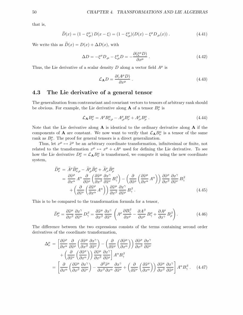
50 CHAPTER 4. TRANSFORMATIONS AND LIE ALGEBRAS
that is,
D(x) = (1 − ξµ,µ)D(x− ξ) = (1 − ξµ
,µ)(D(x) − ξµD,µ(x)) . (4.41)
We write this as D(x) = D(x) + ∆D(x), with
∆D = −ξµD,µ − ξµ,µD = −∂(ξµD)
∂xµ. (4.42)
Thus, the Lie derivative of a scalar density D along a vector field Aµ is
LAD =∂(AµD)
∂xµ. (4.43)
4.3 The Lie derivative of a general tensor
The generalization from contravariant and covariant vectors to tensors of arbitrary rank shouldbe obvious. For example, the Lie derivative along A of a tensor Bµ
ν is
LABµν = AρBµ
ν,ρ −Aµ,ρB
ρν +Aρ
,νBµρ . (4.44)
Note that the Lie derivative along A is identical to the ordinary derivative along A if thecomponents of A are constant. We now want to verify that LAB
µν is a tensor of the same
rank as Bµν . The proof for general tensors is a direct generalization.
Thus, let xµ 7→ xµ be an arbitrary coordinate transformation, infinitesimal or finite, notrelated to the transformation xµ 7→ xµ + ǫAµ used for defining the Lie derivative. To seehow the Lie derivative Dµ
ν = LABµν is transformed, we compute it using the new coordinate
system,
Dµν = AρBµ
ν,ρ − Aµ,ρB
ρν + Aρ
,νBµρ
=∂xρ
∂xαAα ∂
∂xρ
(∂xµ
∂xβ
∂xγ
∂xνBβ
γ
)−(∂
∂xρ
(∂xµ
∂xαAα))
∂xρ
∂xβ
∂xγ
∂xνBβ
γ
+
(∂
∂xν
(∂xρ
∂xαAα))
∂xµ
∂xβ
∂xγ
∂xρBβ
γ . (4.45)
This is to be compared to the transformation formula for a tensor,
Dµν =
∂xµ
∂xβ
∂xγ
∂xνDβ
γ =∂xµ
∂xβ
∂xγ
∂xν
(Aρ ∂B
βγ
∂xρ− ∂Aβ
∂xρBρ
γ +∂Aρ
∂xγBβ
ρ
). (4.46)
The difference between the two expressions consists of the terms containing second orderderivatives of the coordinate transformation,
∆µν =
[∂xρ
∂xα
∂
∂xρ
(∂xµ
∂xβ
∂xγ
∂xν
)−(∂
∂xρ
(∂xµ
∂xα
))∂xρ
∂xβ
∂xγ
∂xν
+
(∂
∂xν
(∂xρ
∂xα
))∂xµ
∂xβ
∂xγ
∂xρ
]AαBβ
γ
=
[∂
∂xα
(∂xµ
∂xβ
∂xγ
∂xν
)− ∂2xµ
∂xβ ∂xα
∂xγ
∂xν+
(∂
∂xν
(∂xρ
∂xα
))∂xµ
∂xβ
∂xγ
∂xρ
]AαBβ
γ . (4.47)
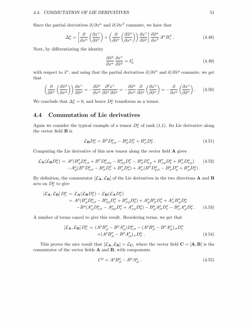
4.4. COMMUTATION OF LIE DERIVATIVES 51
Since the partial derivatives ∂/∂xα and ∂/∂xβ commute, we have that
∆µν =
[∂
∂xα
(∂xγ
∂xν
)+
(∂
∂xν
(∂xρ
∂xα
))∂xγ
∂xρ
]∂xµ
∂xβAαBβ
γ . (4.48)
Next, by differentiating the identity
∂xρ
∂xα
∂xγ
∂xρ= δγ
α (4.49)
with respect to xν , and using that the partial derivatives ∂/∂xν and ∂/∂xρ commute, we getthat
(∂
∂xν
(∂xρ
∂xα
))∂xγ
∂xρ= − ∂xρ
∂xα
∂2xγ
∂xν ∂xρ= − ∂xρ
∂xα
∂
∂xρ
(∂xγ
∂xν
)= − ∂
∂xα
(∂xγ
∂xν
). (4.50)
We conclude that ∆µν = 0, and hence Dµ
ν transforms as a tensor.
4.4 Commutation of Lie derivatives
Again we consider the typical example of a tensor Dµν of rank (1,1). Its Lie derivative along
the vector field B is
LBDµν = BσDµ
ν,σ −Bµ,σD
σν +Bσ
,νDµσ . (4.51)
Computing the Lie derivative of this new tensor along the vector field A gives
LA(LBDµν ) = Aρ(Bσ
,ρDµν,σ +BσDµ
ν,σρ −Bµ,σρD
σν −Bµ
,σDσν,ρ +Bσ
,νρDµσ +Bσ
,νDµσ,ρ) (4.52)
−Aµ,ρ(B
σDρν,σ −Bρ
,σDσν +Bσ
,νDρσ) +Aρ
,ν(BσDµ
ρ,σ −Bµ,σD
σρ +Bσ
,ρDµσ) .
By definition, the commutator [LA,LB] of the Lie derivatives in the two directions A and Bacts on Dµ
ν to give
[LA,LB]Dµν = LA(LBD
µν ) − LB(LAD
µν )
= Aρ(Bσ,ρD
µν,σ −Bµ
,σρDσν +Bσ
,νρDµσ) +Aµ
,ρBρ,σD
σν +Aρ
,νBσ,ρD
µσ
−Bρ(Aσ,ρD
µν,σ −Aµ
,σρDσν +Aσ
,νρDµσ) −Bµ
,ρAρ,σD
σν −Bρ
,νAσ,ρD
µσ . (4.53)
A number of terms cancel to give this result. Reordering terms, we get that
[LA,LB]Dµν = (AρBσ
,ρ −BρAσ,ρ)D
µν,σ − (AρBµ
,ρ −BρAµ,ρ),σD
σν
+(AρBσ,ρ −BρAσ
,ρ),νDµσ . (4.54)
This proves the nice result that [LA,LB] = LC, where the vector field C = [A,B] is thecommutator of the vector fields A and B, with components
Cµ = AρBµ,ρ −BρAµ
,ρ . (4.55)
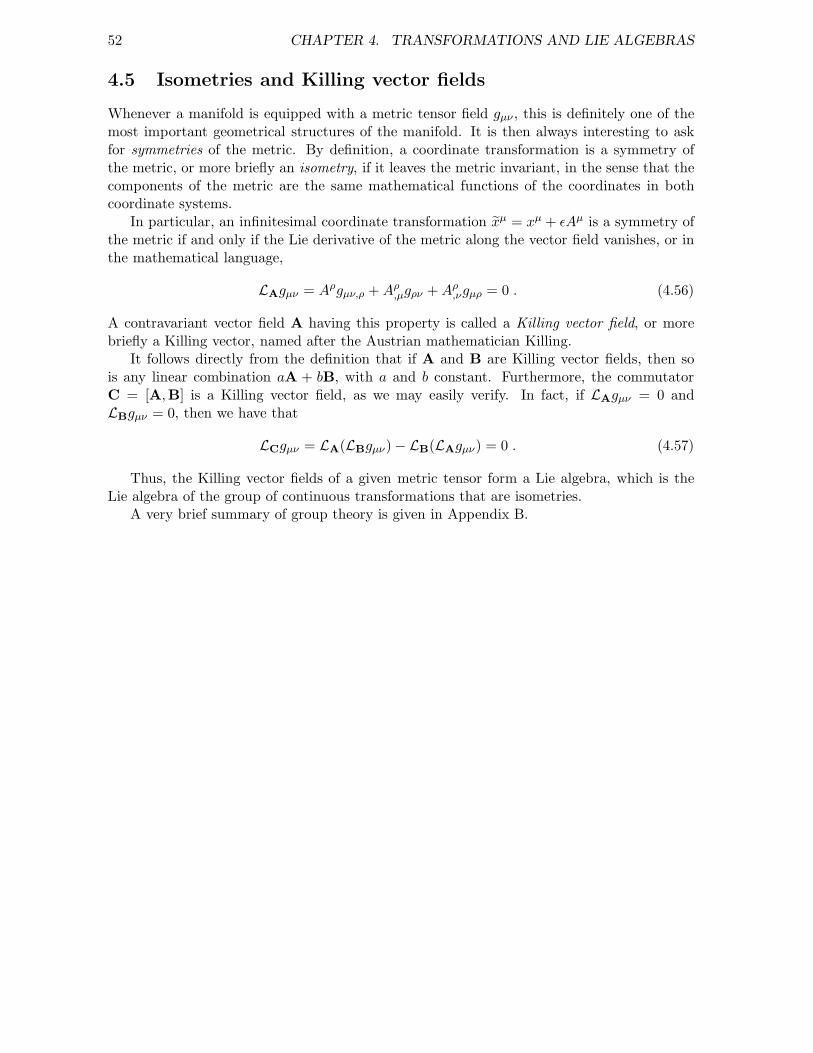
52 CHAPTER 4. TRANSFORMATIONS AND LIE ALGEBRAS
4.5 Isometries and Killing vector fields
Whenever a manifold is equipped with a metric tensor field gµν , this is definitely one of themost important geometrical structures of the manifold. It is then always interesting to askfor symmetries of the metric. By definition, a coordinate transformation is a symmetry ofthe metric, or more briefly an isometry, if it leaves the metric invariant, in the sense that thecomponents of the metric are the same mathematical functions of the coordinates in bothcoordinate systems.
In particular, an infinitesimal coordinate transformation xµ = xµ + ǫAµ is a symmetry ofthe metric if and only if the Lie derivative of the metric along the vector field vanishes, or inthe mathematical language,
LAgµν = Aρgµν,ρ +Aρ,µgρν +Aρ
,νgµρ = 0 . (4.56)
A contravariant vector field A having this property is called a Killing vector field, or morebriefly a Killing vector, named after the Austrian mathematician Killing.
It follows directly from the definition that if A and B are Killing vector fields, then sois any linear combination aA + bB, with a and b constant. Furthermore, the commutatorC = [A,B] is a Killing vector field, as we may easily verify. In fact, if LAgµν = 0 andLBgµν = 0, then we have that
LCgµν = LA(LBgµν) − LB(LAgµν) = 0 . (4.57)
Thus, the Killing vector fields of a given metric tensor form a Lie algebra, which is theLie algebra of the group of continuous transformations that are isometries.
A very brief summary of group theory is given in Appendix B.
4.5. ISOMETRIES AND KILLING VECTOR FIELDS 53
Problems
1. Check explicitly that the Lie derivative of a covariant vector field, as defined in Equa-tion (4.38), transforms as a covariant vector field.
54 CHAPTER 4. TRANSFORMATIONS AND LIE ALGEBRAS
Chapter 5
Differentiation
In the classical theory of fields we encounter many kinds of derivatives, all cousins of thebasic derivative f ′ = df/dx where f is a function of the single variable x. There are timederivatives, gradients, partial derivatives, absolute (or total) derivatives, covariant derivatives,exterior derivatives, divergences, functional derivatives, as well as the Lie derivative alreadyencountered in Chapter 4. We need a variety of notations to keep track of the various kindsof derivatives, and it is not always easy to avoid conflicts in the notation.
5.1 Partial and total derivatives
Time derivatives
The time derivative of a quantity x = x(t) which is a function of time t, is written as
x =dx
dt. (5.1)
If x = x(t) and f = f(x, t) = f(x(t), t), then f has both an explicit time dependence in itssecond argument t, and an implicit time dependence in its first argument x. We distinguishthen between ∂/∂t, partial differentiation, which we apply to the explicit time dependenceonly, and d/dt, called total or absolute differentiation, which we apply to both the explicitand the implicit time dependence. Thus,
f =df
dt=∂f
∂xx+
∂f
∂t. (5.2)
Partial derivatives
We use at least three different notations for the standard partial differentiation of a scalarfunction f = f(x) = f(x0, x1, x2, x3) with respect to one coordinate xµ,
f,µ = ∂µf =∂f
∂xµ. (5.3)
We use occasionally even a fourth notation,
df
dxµ, (5.4)
55
56 CHAPTER 5. DIFFERENTIATION
in the case where f is both an explicit function of x = (x0, x1, x2, x3) and an implicit functionof x through some field φ = φ(x),
f = f(φ(x), x) = f(φ(x0, x1, x2, x3), x0, x1, x2, x3) . (5.5)
Then we may use d/dxµ to denote “absolute partial differentiation”, acting on both theexplicit and the implicit dependence on xµ, whereas we take ∂/∂xµ to act only on the explicitdependence. Thus,
df
dxµ=∂f
∂φ
∂φ
∂xµ+
∂f
∂xµ. (5.6)
5.2 Covariant derivatives of tensor fields
Partial differentiation of a scalar (i.e. a scalar field) gives a covariant vector (i.e. a covariantvector field), since the following formula holds for a coordinate transformation,
φ,µ =∂φ
∂xµ=∂xρ
∂xµ
∂φ
∂xρ=∂xρ
∂xµφ,ρ . (5.7)
Partial differentiation of a vector, on the other hand, does not in general produce a tensor.Thus, for the partial derivatives of a contravariant vector Aµ we have the transformationformula
Aµ,ν =
∂Aµ
∂xν=∂xλ
∂xν
∂
∂xλ
(∂xµ
∂xκAκ)
=∂xλ
∂xν
∂xµ
∂xκAκ
,λ +∂xλ
∂xν
∂2xµ
∂xλ∂xκAκ . (5.8)
The term with second derivatives of the coordinate transformation disqualifies the derivativeAµ
,ν from being called a tensor. One way to avoid the offending term is to admit only linearcoordinate transformations, and that is precisely what we do in the special theory of relativity.Then Aµ
,ν becomes a tensor.A more general method for producing a tensor is to replace the partial differentiation by
a covariant differentiation, which we denote by a semicolon “;” instead of a comma “,”. Wedefine
Aµ;ν = Aµ
,ν + ΓµκνA
κ . (5.9)
The quantities Γλµν are called connection coefficients, and by a coordinate transformation they
are transformed into Γλµν , so that Aµ
;ν is transformed as a tensor,
Aµ;ν = Aµ
,ν + ΓµρνA
ρ =∂xλ
∂xν
∂xµ
∂xκAκ
;λ =∂xλ
∂xν
∂xµ
∂xκ(Aκ
,λ + ΓκσλA
σ) . (5.10)
We see that this equation will hold if
ΓµρνA
ρ =∂xλ
∂xν
∂xµ
∂xκΓκ
σλAσ − ∂xλ
∂xν
∂2xµ
∂xλ∂xκAκ
=∂xλ
∂xν
(∂xµ
∂xκΓκ
σλ − ∂2xµ
∂xλ∂xσ
)∂xσ
∂xρAρ . (5.11)
5.2. COVARIANT DERIVATIVES OF TENSOR FIELDS 57
Since Aρ here is arbitrary, this means that we must define
Γµρν =
∂xσ
∂xρ
∂xλ
∂xν
(∂xµ
∂xκΓκ
σλ − ∂2xµ
∂xλ∂xσ
). (5.12)
For the partial derivatives of a covariant vector field Bµ the following transformationformula holds,
Bµ,ν =∂Bµ
∂xν=
∂
∂xν
(∂xρ
∂xµBρ
)=∂xρ
∂xµ
∂Bρ
∂xν+
∂2xρ
∂xν∂xµBρ
=∂xρ
∂xµ
∂xσ
∂xνBρ,σ +
∂2xρ
∂xν∂xµBρ . (5.13)
Again we define a covariant derivative,
Bµ;ν = Bµ,ν − ∆ρµνBρ , (5.14)
and require ∆ρµν to transform in such a way that Bµ;ν transforms as a tensor,
Bµ;ν = Bµ,ν − ∆ρµνBρ =
∂xκ
∂xµ
∂xλ
∂xνBκ;λ =
∂xκ
∂xµ
∂xλ
∂xν(Bκ,λ − ∆σ
κλBσ) . (5.15)
We see that this equation holds if
∆ρµνBρ =
∂xκ
∂xµ
∂xλ
∂xν∆σ
κλBσ +∂2xρ
∂xν∂xµBρ
=
(∂xκ
∂xµ
∂xλ
∂xν∆σ
κλ +∂2xσ
∂xν∂xµ
)∂xρ
∂xσBρ . (5.16)
This condition holds for an arbitrary Bρ provided that
∆ρµν =
∂xρ
∂xσ
(∂xκ
∂xµ
∂xλ
∂xν∆σ
κλ +∂2xσ
∂xν∂xµ
). (5.17)
The transformation formulae for Γ and ∆ look different, but are in fact identical, because
∂xρ
∂xσ
∂2xσ
∂xν∂xµ=
∂
∂xν
(∂xρ
∂xσ
∂xσ
∂xµ
)−(
∂
∂xν
∂xρ
∂xσ
)∂xσ
∂xµ= −∂x
σ
∂xµ
∂xλ
∂xν
∂2xρ
∂xλ∂xσ. (5.18)
It is therefore very reasonable to choose ∆λµν = Γλ
µν . This choice is not only the simplestpossible, but is necessary if we want covariant differentiation to commute with contraction.See the remark below.
For a tensor with several indices, e.g. Cκλµν , we find by similar computations that the
covariant derivative Cκλµν;ρ transforms as a tensor if we define
Cκλµν;ρ = Cκλ
µν,ρ + ΓκσρC
σλµν + Γλ
σρCκσµν − Γσ
µρCκλσν − Γσ
νρCκλµσ . (5.19)
In particular, the covariant derivative of a scalar field φ is the same as the partial derivative,
φ;ρ = φ,ρ . (5.20)
58 CHAPTER 5. DIFFERENTIATION
This general definition of covariant differentiation implies e.g. that the Leibniz rule holdsfor differentiation of a product of tensors. For example,
(AµBν);ρ = Aµ;ρBν +AµBν;ρ . (5.21)
It implies furthermore that covariant differentiation commutes with contraction. We have forexample that
Aµν;ρ = Aµ
ν,ρ + ΓµσρA
σν − Γσ
νρAµσ , (5.22)
and contraction of the indices µ and ν gives that
Aµµ;ρ = Aµ
µ,ρ + ΓµσρA
σµ − Γσ
µρAµσ = Aµ
µ,ρ = (Aµµ);ρ . (5.23)
The result is the same whether we differentiate first and then contract: Aµν → Aµ
ν;ρ → Aµµ;ρ,
or contract first and then differentiate: Aµν → Aµ
µ → (Aµµ);ρ.
Covariant derivative and Lie derivative
An alternative notation for the covariant derivative of a tensor field C, as in Equation (5.19),is ∇ρC. Given a contravariant vector field A we define the covariant derivative along A as
∇AC = Aρ ∇ρC . (5.24)
It may be interesting to compare the covariant derivative
∇ACκλµν = AρCκλ
µν;ρ = Aρ(Cκλµν,ρ + Γκ
σρCσλµν + Γλ
σρCκσµν − Γσ
µρCκλσν − Γσ
νρCκλµσ) (5.25)
with the Lie derivative as defined in Equation (4.44),
LACκλµν = AρCκλ
µν,ρ −Aκ,σC
σλµν −Aλ
,σCκσµν +Aσ
,µCκλσν +Aσ
,νCκλµσ . (5.26)
The two kinds of derivatives are actually identical if the contravariant vector field A satisfiesthe equation
AρΓκσρ = −Aκ
,σ . (5.27)
If the connection is symmetric, Γκσρ = Γκ
ρσ, then the condition on A is that its covariantderivative vanishes,
Aκ;σ = Aκ
,σ + ΓκρσA
ρ = 0 . (5.28)
We say that the vector field A is parallel, or covariantly constant, when its covariant derivativevanishes.
5.3 Flat and curved space
Tensors from the connection
The connection Γ is not a tensor, or phrased differently, the connection coefficients Γλµν are
not tensor components. The reason is the last term in Equation (5.12), which makes the
5.3. FLAT AND CURVED SPACE 59
transformation formula inhomogeneous when the coordinate transformation is not linear. Bydefinition, tensor components transform homogeneously, which means in particular that zerotransforms into zero.
Since the inhomogeneous term in Equation (5.12) is independent of the connection coeffi-cients, it falls out of the transformation formula for the difference between two connections.Hence, if we vary the connection Γ, then the variation δΓ is a tensor, even though Γ itself isnot.
Because the inhomogeneous term is symmetric in the lower indices it also falls out of thetransformation formula for the torsion, defined as
T λµν = Γλ
µν − Γλνµ . (5.29)
Thus the torsion is a tensor. We say that the connection is symmetric when
T λµν = Γλ
µν − Γλνµ = 0 . (5.30)
This condition is independent of the choice of coordinate system, since the torsion is a tensor.Note that the torsion T λ
µν is a tensor with three indices, not to be confused with theenergy-momentum tensor T µν , having two indices.
Commutation of covariant differentiation
The covariant derivative of a scalar function φ = φ(x) is identical to the usual partial deriva-tive, φ;µ = φ,µ. If we take twice the covariant derivative, we get that
φ;µν = (φ;µ);ν = φ,µν − Γλµνφ,λ . (5.31)
Interchanging the order of the two differentiations gives that
φ;µν − φ;νµ = −(Γλ
µν − Γλνµ
)φ,λ = −T λ
µνφ,λ . (5.32)
Thus, the condition for two covariant differentiations to commute, when applied to an arbi-trary scalar function φ, is that the torsion vanishes, T λ
µν = 0.If we take twice the covariant derivative of a contravariant vector Aκ, we get first that
Aκ;µ = Aκ
,µ + ΓκλµA
λ , (5.33)
and then that
Aκ;µν = (Aκ
;µ);ν = (Aκ;µ),ν + Γκ
ρνAρ;µ − Γσ
µνAκ;σ
= Aκ,µν + Γκ
λµ,νAλ + Γκ
λµAλ
,ν + Γκρν
(Aρ
,µ + ΓρλµA
λ)− Γσ
µνAκ;σ . (5.34)
Interchanging the order of the differentiations gives that
Aκ;µν −Aκ
;νµ = −RκλµνA
λ − T σµνA
κ;σ , (5.35)
where we have defined
Rκλµν = Γκ
λν,µ − Γκλµ,ν + Γκ
ρµΓρλν − Γκ
ρνΓρλµ . (5.36)
Since all the other quantities in Equation (5.35) are tensors, and since the vector Aκ isarbitrary, it follows that Rκ
λµν is a tensor. It is called the curvature tensor, and we willexamine it more closely in Chapter 6. We see that both the torsion tensor T σ
µν and thecurvature tensor Rκ
λµν measure by how much covariant differentiations in different directionsfail to commute.
60 CHAPTER 5. DIFFERENTIATION
Flat space
That spacetime (or “timespace”) is flat, means by definition that there exists at least onecoordinate system in which the connection is trivial, Γκ
λµ = 0. In this particular coordinatesystem, covariant derivation reduces to ordinary partial differentiation, and the torsion andcurvature tensors both vanish, T κ
λµ = 0 and Rκλµν = 0. But the torsion and curvature
tensor are tensors, therefore they vanish in every coordinate system if they vanish in one.If the connection coefficients Γκ
λµ do not vanish identically, we may learn whether ornot spacetime is flat by looking at the torsion and the curvature tensor. The characteristicproperty of a flat manifold is that T κ
λµ = 0 and Rκλµν = 0, so that covariant differentiations
in different directions commute. These two conditions are necessary for flatness, as remarkedabove, and are actually also sufficient, even though the sufficiency is somewhat less obvious.We will not prove here that spacetime is flat if the torsion and curvature vanish.
In order to see in a different way the significance of the two conditions T κλµ = 0
and Rκλµν = 0, consider the transformation formula for the connection coefficients, Equa-
tion (5.12). If we try to transform away a given connection Γκλµ, that is, to find new coordinates
xµ such that Γκλµ = 0, we have the following set of second order partial differential equations
to solve,
∂xµ
∂xκΓκ
σλ − ∂2xµ
∂xλ∂xσ= 0 . (5.37)
Since partial derivatives always commute, the symmetry condition Γκσλ = Γκ
λσ, or equivalently,T κ
σλ = 0, is necessary for the existence of four independent solutions x0, x1, x2 and x3.This is however not the whole story, since we may differentiate Equation (5.37). We get
then first that
∂3xµ
∂xρ∂xλ∂xσ=
∂2xµ
∂xρ∂xκΓκ
σλ +∂xµ
∂xκΓκ
σλ,ρ . (5.38)
Here we may use Equation (5.37) to eliminate the second derivatives of xµ, this gives that
∂3xµ
∂xρ∂xλ∂xσ=∂xµ
∂xκ
(Γκ
αρΓασλ + Γκ
σλ,ρ
). (5.39)
The left hand side of this equation is symmetric in all the three indices ρ, λ and σ, and sothe right hand side must have the same symmetry. That the right hand side is symmetric inλ and σ, is no new condition. But a new necessary condition for solution is that the righthand side must be symmetric in ρ and λ. The symmetry must hold without restrictions onthe derivatives ∂xµ/∂xκ, and the resulting condition is that Rκ
σρλ = 0.
Curved spacetime and Einstein’s principle of equivalence
When the connection is symmetric, then it is always possible to choose the coordinates x suchthat Γκ
λµ = 0 at any single given point. In fact, this is only a question of choosing suitablevalues for the first and second derivatives of the coordinate transformation x 7→ x at this onepoint, so that Equation (5.37) holds there.
The postulate that such a coordinate system exists at any given point, is one possibleformulation of Einstein’s principle of equivalence in the general theory of relativity. Themathematical formulation of the principle of equivalence is that the connection must besymmetric, Γκ
λµ = Γκµλ.
5.4. METRIC CONNECTION 61
5.4 Metric connection
Covariant derivation can be defined independent of the metric, but the two concepts fit neatlytogether if we require that covariant differentiation should commute with raising and loweringof indices, like it commutes with contraction. If for example Aµ = gµνA
ν , then
Aµ;ρ = (gµνAν);ρ = gµν;ρA
ν + gµνAν;ρ , (5.40)
according to the Leibniz rule. We now require that we get the same result by differentiatingfirst and lowering the index afterwards, i.e. that
Aµ;ρ = gµνAν;ρ . (5.41)
If this is to hold for an arbitrary vector field Aν , a necessary and sufficient condition is thatthe covariant derivative of the metric vanishes,
gµν;ρ = gµν,ρ − gσνΓσµρ − gµσΓσ
νρ = 0 . (5.42)
An equivalent condition is that
gµν;ρ = gµν
,ρ + gσνΓµσρ + gµσΓν
σρ = 0 . (5.43)
Depending on whether we regard this as a condition on the metric or on the connection, wesay either that the metric is covariantly constant, or that the connection is metric.
A metric connection is uniquely given by the metric tensor and its derivatives, and by thetorsion. In order to deduce the relation we write the equation gµν;ρ = 0 three times with thesame indices in different orders, as follows,
gµν,ρ = gσνΓσµρ + gµσΓσ
νρ ,
gρµ,ν = gσµΓσρν + gρσΓσ
µν , (5.44)
gνρ,µ = gσρΓσνµ + gνσΓσ
ρµ .
This gives that
gρµ,ν + gνρ,µ − gµν,ρ = gρσ(2Γσµν − T σ
µν) + gµσTσ
ρν + gνσTσ
ρµ , (5.45)
when we use the symmetry of the metric tensor and the definition of the torsion, Equa-tion (5.29). We multiply this equation by gλρ, and write Tρµν = gρσT
σµν , then we get that
Γλµν =
1
2gλρ(gρµ,ν + gνρ,µ − gµν,ρ + Tρµν + Tµνρ + Tνµρ) . (5.46)
We may easily verify that this connection is metric, without other restrictions on the torsionthan the antisymmetry Tρµν = −Tρνµ, which holds by definition. Note that the torsion is notjust the antisymmetric part of the connection, but also contributes to the symmetric part ofa metric connection, unless it is antisymmetric in the first two indices so that
Tµνρ + Tνµρ = 0 . (5.47)
In this case it is completely antisymmetric,
Tρµν = −Tρνµ = Tνρµ = −Tνµρ = Tµνρ = −Tµρν . (5.48)
62 CHAPTER 5. DIFFERENTIATION
If the connection is symmetric, Γλµν = Γλ
νµ, as well as metric, it is uniquely given by themetric as
Γλµν =
1
2gλρ(gρµ,ν + gνρ,µ − gµν,ρ) . (5.49)
This unique symmetric and metric connection is called the Christoffel connection. It is usedin the general theory of relativity, where the metric tensor represents the gravitational field.
For later reference, let us compute the derivative Γκλµ,ν for the metric and symmetric
connection. Equation (5.49) together with Equation (5.43) gives that
Γκλµ,ν =
1
2gκρ(gρλ,µν + gρµ,λν − gλµ,ρν) +
1
2gκρ
,ν(gρλ,µ + gρµ,λ − gλµ,ρ)
=1
2gκρ(gρλ,µν + gρµ,λν − gλµ,ρν) − (gσρΓκ
σν + gκσΓρσν) gρτ Γτ
λµ (5.50)
=1
2gκρ(gρλ,µν + gρµ,λν − gλµ,ρν) − Γκ
σνΓσλµ − gκρgστΓσ
ρνΓτλµ .
5.5 Covariant divergence
The covariant divergence of a contravariant vector field Aµ = Aµ(x) is
Aµ;µ = Aµ
,µ + ΓµρµA
ρ . (5.51)
This expression can be simplified when the connection is symmetric and metric. Equa-tion (5.49) gives that
Γµρµ =
1
2gµσgσµ,ρ =
1
2gg,ρ =
1√|g|
∂
∂xρ
√|g| =
1
2
∂
∂xρln |g| , (5.52)
when we recall the definition
g = det(gµν) , (5.53)
and use Equation (2.79). We write |g| in order to cover the case g < 0. This allows us towrite
Aµ;µ =
1√|g|
∂
∂xµ
(√|g|Aµ
). (5.54)
An important special case is when φ is a scalar field, and Aµ = gµνφ,ν . Then we have that
gµνφ;νµ = Aµ;µ =
1√|g|
∂
∂xµ
(√|g| gµν ∂φ
∂xν
). (5.55)
This formula defines the Laplace–Beltrami operator,
∆ =1√|g|
∂
∂xµ
√|g| gµν ∂
∂xν, (5.56)

5.6. EXTERIOR DERIVATIVES OF FORMS 63
which generalizes the Laplace operator defined in Equation (1.10). The present definitionapplies to an arbitrary metric in an arbitrary coordinate system.
The d’Alembert operator in four dimensions,
2 =1
c2∂2
∂t2− ∂2
∂x2− ∂2
∂y2− ∂2
∂z2, (5.57)
is the special case of the Laplace–Beltrami operator when the metric is
ds2 = c2dt2 − dx2 − dy2 − dz2 . (5.58)
There is a similar simplification when we compute the covariant divergence of a con-travariant antisymmetric tensor of arbitrary rank, always under the condition that the con-nection is both symmetric and metric. For example, for an antisymmetric tensor of rank two,Aµν = −Aνµ, we have that
Aµν;ν = Aµν
,ν + ΓµρνA
ρν + ΓνρνA
µρ =1√|g|
∂
∂xν(√|g|Aµν) . (5.59)
We use here that ΓµρνA
ρν = 0 when Γµρν is symmetric and Aρν antisymmetric in the indices
ρ, ν.An important example is the four Maxwell equations with sources, having the following
form in a general coordinate system,
Fµν;ν = −µ0j
µ . (5.60)
Or equivalently,
∂
∂xν
(√|g|Fµν
)= −µ0
√|g| jµ . (5.61)
5.6 Exterior derivatives of forms
The commutator of two contravariant vector fields, as defined in Equation (2.36) and (2.37), isan example showing that it is possible to make a tensor by differentiation of a vector withoutusing covariant differentiation.
The covariant derivative is also not the only tensor we may produce from the partialderivatives Bµ,ν of a covariant vector field Bµ. In fact, we get another tensor simply byantisymmetrizing in the indices µ and ν. We define the exterior derivative of Bµ as
(dB)µν = 2∂[µBν] = 2B[ν,µ] = Bν,µ −Bµ,ν , (5.62)
and Equation (5.13) shows that it transforms as a tensor,
B[ν,µ] =∂xσ
∂xν
∂xρ
∂xµB[σ,ρ] . (5.63)
For example,
∇× B =
(∂Bz
∂y− ∂By
∂z
)i +
(∂Bx
∂z− ∂Bz
∂x
)j +
(∂By
∂x− ∂Bx
∂y
)k (5.64)

64 CHAPTER 5. DIFFERENTIATION
is the exterior derivative of a three dimensional vector B = Bxi +Byj +Bzk.Another example is the relation between the field tensor Fµν and the four dimensional
vector potential Aµ in electromagnetism,
Fµν = (dA)µν = Aν,µ −Aµ,ν . (5.65)
We may define quite generally an exterior differentiation of forms which is coordinateindependent, and yet involves nothing but standard partial derivatives. Recall that an n-form is the same as an antisymmetric covariant tensor of rank n. The exterior derivative ofan n-form Bκλ...ν is an (n+ 1)-form
(dB)ρκλ...ν = (n+ 1)B[κλ...ν,ρ] . (5.66)
The right hand side of this equation is by definition antisymmetric in all its n + 1 indices.That it transforms as a tensor, follows in a similar way as in the special case n = 1 above. Inthe special case n = 0 the exterior derivative equals the usual partial derivative,
(dB)ρ = B,ρ . (5.67)
We have previously introduced a special notation for forms, writing
B =1
n!Bκλ...ν dxκ ∧ dxλ ∧ . . . ∧ dxν ,
dB =1
(n+ 1)!(dB)ρκλ...ν dxρ ∧ dxκ ∧ dxλ ∧ . . . ∧ dxν . (5.68)
The definition in Equation (5.66) means that
dB =
(1
n!Bκλ...ν,ρ dxρ
)∧ dxκ ∧ dxλ ∧ . . . ∧ dxν . (5.69)
In particular, the exterior derivative of a 2-form Bκλ is
(dB)ρκλ = 3B[κλ,ρ] =1
2(Bκλ,ρ +Bρκ,λ +Bλρ,κ −Bλκ,ρ −Bκρ,λ −Bρλ,κ)
= Bκλ,ρ +Bρκ,λ +Bλρ,κ . (5.70)
And the exterior derivative of a 3-form Bκλµ is
(dB)ρκλµ = 4B[κλµ,ρ] = Bκλµ,ρ −Bρκλ,µ +Bµρκ,λ −Bλµρ,κ . (5.71)
5.7 Poincare’s lemma, magnetic monopoles
Twice exterior differentiation gives identically zero, d2 = 0, because partial differentiationscommute,
(d2B)σρκλ...ν = (n+ 2)(dB)[ρκλ...ν,σ] = (n+ 2)(n + 1)B[κλ...ν,ρσ] = 0 . (5.72)
In general we say that an n-form B is closed if dB = 0, and is exact if B = dA for some(n− 1)-form A. An exact form dA is always closed, since d2A = 0.
5.7. POINCARE’S LEMMA, MAGNETIC MONOPOLES 65
The converse result, that a closed form is always exact, is called Poincare’s lemma. Itholds in the d dimensional Euclidean space Rd. It holds also locally in an arbitrary manifoldof dimension d, in the sense that around any given point there is always some open neigh-bourhood in which all closed forms are exact. However, it may not hold globally in a manifoldwith a non-trivial topology.
Poincare’s lemma will hold for example for all closed 1-forms in some region if that region issimply connected, which means that every continuous closed curve is continuously deformableinto a point. In the case of n-forms, the condition is that every closed surface of dimensionn should be continuously deformable into a point. A couple of examples will illustrate whatmay sometimes go wrong.
Example: n = 1
Puncture the (x, y) plane by removing the origin (x, y) = (0, 0). The polar coordinates (r, ϕ)are well defined by the relations x = r cosϕ, y = r sinϕ, although the angle ϕ is multivalued.We have that
dx = cosϕ dr − r sinϕ dϕ ,
dy = sinϕ dr + r cosϕ dϕ , (5.73)
and inversely,
dr = cosϕ dx+ sinϕ dy =x dx+ y dy√
x2 + y2,
dϕ = −sinϕ
rdx+
cosϕ
rdy =
−y dx+ x dy
x2 + y2. (5.74)
The 1-form
B = Bx dx+By dy =x√
x2 + y2dx+
y√x2 + y2
dy (5.75)
is closed, as we may verify by computation,
dB =
(∂Bx
∂xdx+
∂Bx
∂ydy
)∧ dx+
(∂By
∂xdx+
∂By
∂ydy
)∧ dy
=
(∂By
∂x− ∂Bx
∂y
)dx ∧ dy = 0 . (5.76)
It is also exact, since B = dr, and r =√x2 + y2 is a single valued function in the punctured
plane, not only continuously differentiable but even analytic.The 1-form
C = Cx dx+ Cy dy = − y
x2 + y2dx+
x
x2 + y2dy (5.77)
is also closed,
dC =
(∂Cy
∂x− ∂Cx
∂y
)dx ∧ dy = 0 . (5.78)

66 CHAPTER 5. DIFFERENTIATION
It is exact in the sense that C = dϕ. However, ϕ is not a single valued function in the wholepunctured plane, it is multivalued because it increases by 2π when we go once around theorigin in the anticlockwise direction. We do not accept multivalued functions, therefore wedo not accept C as an exact 1-form. Note that the derivative dϕ is single valued, even thoughϕ is multivalued.
The root of the problem is that the punctured plane is not simply connected: a loop aroundthe origin can not be continuously deformed into a point. To obtain a simply connected regionwe may for example cut the plane by removing the negative x axis. Then what remains is asimply connected region where the angle ϕ = ϕ(x, y) is a single valued function,
ϕ(x, y) = 2 arctan
(y
r + x
), (5.79)
and where the 1-form C = dϕ is exact.
Example: n = 2, magnetic monopole field
Consider a static (time independent) magnetic flux density in three dimensions,
B = Bx i +By j +Bz k . (5.80)
The equation
∇ · B =∂Bx
∂x+∂By
∂y+∂Bz
∂z= 0 (5.81)
is one of Maxwell’s equations. It says that no magnetic charges exist that are sources of themagnetic field. We solve it by introducing a vector potential A such that
B = ∇× A . (5.82)
A different description of the same reality is to treat the magnetic flux density as a 2-form,
B = Bx dy ∧ dz +By dz ∧ dx+Bz dx ∧ dy . (5.83)
Then the same Maxwell’s equation takes the form dB = 0, since
dB = dBx ∧ dy ∧ dz + dBy ∧ dz ∧ dx+ dBz ∧ dx ∧ dy
=
(∂Bx
∂xdx+
∂Bx
∂ydy +
∂Bx
∂zdz
)∧ dy ∧ dz
+
(∂By
∂xdx+
∂By
∂ydy +
∂By
∂zdz
)∧ dz ∧ dx
+
(∂Bz
∂xdx+
∂Bz
∂ydy +
∂Bz
∂zdz
)∧ dx ∧ dy (5.84)
=
(∂Bx
∂x+∂By
∂y+∂Bz
∂z
)dx ∧ dy ∧ dz .
Since the 2-form B is closed, by Poincare’s lemma it is also exact, which means that thereexists a 1-form
A = Ax dx+Ay dy +Az dz (5.85)
5.7. POINCARE’S LEMMA, MAGNETIC MONOPOLES 67
such that
B = dA = dAx ∧ dx+ dAy ∧ dy + dAz ∧ dz
=
(∂Az
∂y− ∂Ay
∂z
)dy ∧ dz +
(∂Ax
∂z− ∂Az
∂x
)dz ∧ dx+
(∂Ay
∂x− ∂Ax
∂y
)dx ∧ dy . (5.86)
The Maxwell equation ∇ · B = 0, or dB = 0, forbids magnetic charges. But if we nowpuncture the three dimensional space by removing the origin, then we are free to place amagnetic monopole at the origin, so as to get the field
Bx =kx
r3, By =
ky
r3, Bz =
kz
r3, (5.87)
where k is a konstant, and r =√x2 + y2 + z2. We easily verify that dB = 0 for r > 0. Hence,
by Poincare’s lemma, there exists at least locally a vector potential A such that B = dA.The equation for A is most easily solved in polar coordinates r, θ, ϕ, defined by the relations
x = r sin θ cosϕ , y = r sin θ sinϕ , z = r cos θ . (5.88)
From these follows that
dx = sin θ cosϕ dr + r cos θ cosϕ dθ − r sin θ sinϕ dϕ ,
dy = sin θ sinϕ dr + r cos θ sinϕ dθ + r sin θ cosϕ dϕ , (5.89)
dz = cos θ dr − r sin θ dθ ,
and altogether we find that
B =k
r3(xdy ∧ dz + y dz ∧ dx+ z dx ∧ dy) = k sin θ dθ ∧ dϕ . (5.90)
See Problem 6. Thus, the equation dA = B has the following three components in polarcoordinates,
∂Ar
∂θ− ∂Aθ
∂r= 0 ,
∂Ar
∂ϕ− ∂Aϕ
∂r= 0 ,
∂Aϕ
∂θ− ∂Aθ
∂ϕ= k sin θ . (5.91)
The simplest solution is
A = −k cos θ dϕ =kz(y dx− xdy)
r(x2 + y2). (5.92)
This is singular at x2 + y2 = 0, corresponding to θ = 0 and θ = π in polar coordinates.Another solution, which is singular at θ = π but not at θ = 0, is
A = k(1 − cos θ) dϕ =k(r − z)(xdy − y dx)
r(x2 + y2)=k(xdy − y dx)
r(r + z). (5.93)
Thus, by removing the negative z axis we obtain a region in which the closed 2-form B isexact.
68 CHAPTER 5. DIFFERENTIATION
5.8 Divergence of densities
Let Aµ be a vector density in four dimensions. Then its dual,
Aαβγ = ǫµαβγ Aµ , (5.94)
is a 3-form, the exterior derivative of which is a 4-form,
(dA)δαβγ = 4(A)[αβγ,δ] = 4ǫµ[αβγAµ
,δ] . (5.95)
Finally the dual of this 4-form is a scalar density,
(dA) =1
24ǫδαβγ (dA)δαβγ =
1
6ǫδαβγ ǫµ[αβγA
µ,δ]
=1
6ǫδαβγ ǫµαβγA
µ,δ = Aδ
,δ . (5.96)
We see that by taking first the dual of a vector density, next the exterior derivative andfinally the dual once more, we get the divergence of the original vector density, with standardpartial derivatives and not covariant derivatives. This divergence is a scalar density, as isproved by our computation via the exterior differentiation.
As another example, let Aµν be a 2-density, i.e. an antisymmetric tensor density of ranktwo. The dual,
Aαβ =1
2ǫµναβ A
µν , (5.97)
is a 2-form, the exterior derivative of which is a 3-form,
(dA)γαβ = 3(A)[αβ,γ] =3
2ǫµν[αβ A
µν,γ] , (5.98)
the dual of which is in turn a vector density,
(dA)κ =1
6ǫκγαβ (dA)γαβ =
1
4ǫκγαβ ǫµν[αβ A
µν,γ]
=1
4ǫκγαβ ǫµναβ A
µν,γ = Aκγ
,γ . (5.99)
In general, when A is an n-density, and we compute its divergence by standard partialdifferentiation, we get an (n−1)-density, which we may call divA. We see that the operation
div = d (5.100)
is invariant under arbitrary coordinate transformations, when it acts on densities, withoutinvolving either connection or metric.
The left hand side of Equation (5.61), Maxwell’s equation, is the divergence of a 2-density,hence it is a 1-density. Since the right hand side is also a 1-density, the left and right handsides both transform in the same way, and the equation is invariant under general coordinatetransformations.

5.8. DIVERGENCE OF DENSITIES 69
The Laplace–Beltrami operator rederived
When we define the divergence of a vector density as above, and in addition invoke the metric,we are in a position to rediscover the Laplace–Beltrami operator defined in Equation (5.56),
∆ =1√|g|
∂
∂xµ
√|g| gµν ∂
∂xν. (5.101)
When it acts on a scalar function φ = φ(x) = φ(x0, x1, x2, x3), the result ∆φ is again a scalarfunction, and a simple proof is the following. First we have that
Aν = φ,ν =∂φ
∂xν(5.102)
is a covariant vector, therefore Bµ = gµνAν is a contravariant vector and Cµ =√|g|Bµ a
vector density. The divergence of this vector density,
D = Cµ,µ =
∂Cµ
∂xµ, (5.103)
is a scalar density, and finally ∆φ = D/√|g| is a scalar, as we wanted to prove.
We have already derived the same operator from the covariant differentiation with a metricand symmetric connection. Later on, we are going to derive it a third time, starting from aninvariant variational principle for a scalar field, the Klein–Gordon field.
70 CHAPTER 5. DIFFERENTIATION
Problems
1. Show that the two conditions (5.42) and (5.43) are equivalent definitions of a covariantlyconstant metric (or of a metric connection). That is, if one of them holds, then the otherone follows.
2. Express the Laplace–Beltrami operator ∆ in the plane both in the Cartesian coordinates(x, y) and in the polar coordinates (r, ϕ).Use the results from Problem 3 in Chapter 2, and compare with Equation (1.81).
3. Express the Laplace–Beltrami operator in the three dimensional Cartesian coordinates(x, y, z) and in the polar coordinates (r, θ, ϕ).Use the results from Problem 4 in Chapter 2, and compare with Problem 1 in Chapter 1.
4. Write in polar coordinates (θ, ϕ) the Laplace–Beltrami operator ∆ on the surface of thesphere, using the metric found in Problem 5 in Chapter 2.
5. As an example of the commutation of covariant differentiation in different directions,show in general that for a covariant tensor Aκλ of rank two we have
Aκλ;µν −Aκλ;νµ = Rρκµν Aρλ +Rρ
λµν Aκρ − T ρµν Aκλ;ρ .
Take Aκλ = gκλ in this relation, and show that if the connection is metric, i.e. ifgκλ;µ = 0, then the curvature tensor is antisymmetric in the two first indices, i.e.Rκλµν = −Rλκµν , when we define Rκλµν = gκρR
ρλµν .
6. Verify the second equality in Equation (5.90).Hint: to simplify the computation, use e.g. that
xdy ∧ dz + y dz ∧ dx = (x dy − y dx) ∧ dz .
Chapter 6
Parallel transport and curvature
We saw in Chapter 5 that covariant differentiations in two different directions do not alwayscommute, unless both the torsion tensor and the curvature tensor vanish. In this chapter wewill study the curvature tensor from a slightly different mathematical point of view.
In the general theory of relativity the torsion in the physical spacetime is assumed tovanish identically. The physical meaning of the curvature tensor is that it is nonzero in thepresence of a gravitational field, and it represents the gravitational field in Einstein’s equation,as we shall see in Chapter 16.
Covariant differentiation defines in a coordinate independent way what it means that avector field is constant along a given curve. In other words, covariant differentiation defineshow to parallel transport a vector along a curve. Conversely, we may define covariant dif-ferentiation by means of parallel transport, so in this sense the two concepts are equivalent.The curvature tensor describes what happens when we parallel transport a vector around aninfinitesimal closed curve.
Parallel transport of vectors gives meaning to the concept of straight lines. Quite literally,a line is straight if it has a constant direction, i.e. if the tangent vectors at all points onthe curve are parallel. Straight lines are also called geodesic lines, or geodesics for short. Ageodesic line on the surface of a sphere, in particular, is called a great circle. The equationsaying that all tangent vectors along a curve are parallel, is called the geodesic equation, itinvolves the connection and no other geometric quantities.
Another well known characteristic of a straight line is that it is the shortest route betweentwo points, or sometimes actually the longest route, in any case a route of extremal length.This property of a geodesic is in fact a variational principle from which we may derive thegeodesic equation, as we will do in Chapter 15. The connection occurring in the geodesicequation as derived from the variational principle, may be defined to be symmetric, and isthen uniquely defined by the metric.
If we have both a metric and a connection, then we have two ways of deriving a geodesicequation, and we have to ask whether the two methods produce the same equation. We saythat the connection is metric, or that the metric is covariantly constant, when the metric andthe connection are compatible in this way. It turns out that an equivalent condition is thatthe parallel transport of a vector always preserves the length of the vector.
71
72 CHAPTER 6. PARALLEL TRANSPORT AND CURVATURE
6.1 Parallel transport of vectors and tensors
Let Aµ = Aµ(x) = Aµ(x0, x1, x2, x3) be a contravariant vector field. Given a curve xµ = xµ(u),the vector field along the curve is a function of the curve parameter u, i.e. Aµ = Aµ(u) =Aµ(x(u)), and we may differentiate the components Aµ with respect to u,
dAµ
du=∂Aµ
∂xρ
dxρ
du= Aµ
,ρdxρ
du. (6.1)
Here dxρ/du are the components of the tangent vector to the curve. If dAµ/du = 0, then thecomponents of the vector field are constant along the curve. However, that the componentsare constant does not necessarily mean that the vector is constant. In our definition of aconstant vector field we want a criterion which does not depend on the coordinate system,and in this respect the criterion of constant components is unacceptable.
By definition, the vector field Aµ = Aµ(x) is constant along the curve x = x(u), or inother words, all the vectors Aµ = Aµ(u) = Aµ(x(u)) along the curve are parallel, if
Aµ;ρ
dxρ
du=(Aµ
,ρ + ΓµσρA
σ) dxρ
du= 0 . (6.2)
This condition may be rewritten in the following way, making it clear that it involves onlythe vector field along the curve,
dAµ
du+ Γµ
σρAσ dxρ
du= 0 . (6.3)
Given an initial condition Aµ(u) = Cµ at one parameter value u = u0 this equation has aunique solution Aµ(u), which is, by definition, the parallel transport of the vector Cµ alongthe curve.
By a similar reasoning we find the equation for parallel transport of a covariant vector Bµ
along a curve,
dBµ
du− Γσ
µρBσdxρ
du= 0 . (6.4)
The definition is easily extended to the parallel transport of any tensor.The two equations (6.3) and (6.4) together imply e.g. that if the contravariant vectors
Aµ = Aµ(u) are parallel along the curve x(u), and the covariant vectors Bµ = Bµ(u) areparallel as well, then the scalar quantity AµBµ is constant along the curve,
d(AµBµ)
du=
dAµ
duBµ +Aµ dBµ
du= −Γµ
σρAσ dxρ
duBµ +AµΓσ
µρBσdxρ
du= 0 . (6.5)
We may multiply Equation (6.3) by du to rewrite it as
dAµ = −ΓµσρA
σ dxρ . (6.6)

6.1. PARALLEL TRANSPORT OF VECTORS AND TENSORS 73
In this form, the equation is explicitly independent of the curve parameter u, and shows thusthat the parallel transport along a curve is independent of how the curve is parametrized. Itsays that a contravariant vector Aµ at a point x is parallel to the vector
Aµ + dAµ =(δµσ − Γµ
σρ dxρ)Aσ (6.7)
at the infinitesimally close point x+ dx. Similarly, we may write Equation (6.4) in the form
dBµ = ΓσµρBσ dxρ , (6.8)
saying that the covariant vector Bµ at x is parallel to the following vector at x+ dx,
Bµ + dBµ =(δσµ + Γσ
µρ dxρ)Bσ . (6.9)
We have now defined what is meant by parallel vectors, whether they are contravariantor covariant. The definition is coordinate independent, but on the other hand it is curvedependent. In order to compare two vectors localized at separate points in space and time, wehave to parallel transport the vector from one point along some curve to the other point. Ina flat space the result of a parallel transport depends only on the start and end points and isindependent of the curve. But in a curved space the parallel transport along different curveswill give different results. Only infinitesimal parallel transport, as given by Equation (6.7)for a contravariant vector and by Equation (6.9) for a covariant vector, is uniquely defined ina curved space.
The geodesic equation
The most direct definition of a straight line is that it has a constant direction. More precisely,it has a constant unit tangent vector dxµ/ds, where s = s(u) is a special curve parametermeasuring the distance along the curve, called the arc length. Inserting Aµ = dxµ/ds inEquation (6.3) gives the geodesic equation,
d
du
(dxµ
ds
)+ Γµ
σρ
dxσ
ds
dxρ
du= 0 . (6.10)
Multiplying the equation by du/ds gives it the following standard form,
d2xµ
ds2+ Γµ
σρ
dxσ
ds
dxρ
ds= 0 . (6.11)
Note that the geodesic equation defines the curve in terms of a special parameter s whichis proportional to the arc length measured along the curve from an arbitrary starting point.In fact, the parameter is unique up to two arbitrary constants, since s′ = λ(s − s0) is anequally good parameter when s0 is an arbitrary zero point and λ an arbitrary scale factor.
74 CHAPTER 6. PARALLEL TRANSPORT AND CURVATURE
The geodesic equation determines distances along a geodesic, up to a proportionality constant,independent of the existence of a metric.
Note also that it is only the symmetric part of the connection that contributes in thegeodesic equation. The torsion, which is the antisymmetric part of the connection, does notcontribute.
Metric connection
Given both a connection Γλµν and a metric gµν , it is natural to ask whether the parallel
transport of a vector preserves its length. Equation (6.3) implies that
d
du(gµνA
µAν) =(gµν,ρ − gσνΓσ
µρ − gµσΓσνρ
) dxρ
duAµAν = gµν;ρ
dxρ
duAµAν . (6.12)
Thus, the length of an arbitrary contravariant vector is preserved under parallel transport ifand only if gµν;ρ = 0.
We have seen this condition, the vanishing of the covariant derivative of the metric tensor,already in Chapter 5. When it holds, we say either that the metric is covariantly constant,or that the connection is metric. We found that for a given metric tensor field there exists aunique connection which is symmetric and metric. As we shall see in Chapter 15, the geodesicequation as derived from a variational principle contains again the unique symmetric andmetric connection.
6.2 Covariant differentiation from parallel transport
We have used above the concept of covariant differentiation in order to define the paralleltransport of vectors. We will now see how to go the other way, from parallel transport tocovariant differentiation.
Partial differentiation of the components Aµ = Aµ(x) of a contravariant vector field A =A(x) amounts to a comparison of the components Aµ(x) and Aµ(x+dx) at two infinitesimallynearby points x and x+ dx. The partial derivatives Aµ
,ν are defined by the relation
Aµ(x+ dx) = Aµ(x) +Aµ,ν(x) dxν , (6.13)
valid for an arbitrary infinitesimal dx. However, these derivatives are not covariant, becausethe definition is coordinate dependent, or phrased differently, Aµ
,ν is not a tensor undernon-linear coordinate transformations.
The basic problem is that we try to compare quantities that are not directly comparable:the vectors A(x) and A(x + dx) localized at the two different points x and x + dx. A wayto compare them which makes better sense is to parallel transport one vector to the otherpoint, and this is how we define the covariant derivatives Aµ
;ν. By definition, the vectorAµ(x) + Aµ
;ν(x) dxν is located at x, and in order to compare it with the vector Aµ(x + dx)located at x, we have to parallel transport it from x to x+ dx. Thus, the equation definingthe covariant differentiation looks as follows,
Aµ(x+ dx) =(δµρ − Γµ
ρσ dxσ)
(Aρ(x) +Aρ;ν(x) dxν)
= Aµ(x) +(Aµ
;ν(x) − ΓµρνA
ρ(x))
dxν . (6.14)

6.3. TORSION AND CURVATURE 75
We put (dx)2 = 0 here because dx is infinitesimal. The present definition of Aµ;ν(x) means
that it is tensor localized at x. Comparison between the two equations above gives that
Aµ;ν = Aµ
,ν + ΓµρνA
ρ . (6.15)
The covariant derivative Bµ;ν of a covariant vector field Bµ = Bµ(x) is defined in a similarway, by the relations
Bµ(x+ dx) = Bµ(x) +Bµ,ν(x) dxν
=(δλµ + Γλ
µσ dxσ)
(Bλ(x) +Bλ;ν(x) dxν) (6.16)
= Bµ(x) +(Bµ;ν(x) + Γλ
µνBλ(x))
dxν .
This gives that
Bµ;ν = Bµ,ν − ΓλµνBλ . (6.17)
The generalization to tensors of arbitrary rank should be obvious.
6.3 Torsion and curvature
The torsion and curvature tensors both have clear geometric interpretations in terms of par-allel transport. The torsion measures by how much an infinitesimal parallellogram fails tobe closed, whereas the curvature tensor measures how much the parallel transport of vectorsbetween two points, or from one point back to the same point, depends on the curve.
The torsion tensor
We obtain an infinitesimal parallellogram with one corner at the point x in the following way.Let dx and dy be the two infinitesimal sides meeting at x. We parallel transport dy alongdx, the result is
dyλ = dyλ − Γλµν dyµ dxν . (6.18)
Then we parallel transport dx along dy, with the result
dxλ = dxλ − Γλµν dxµ dyν . (6.19)
What then lacks for the parallellogram to close, is
dxλ + dyλ −(dyλ + dxλ
)= T λ
µν dxµ dyν . (6.20)
76 CHAPTER 6. PARALLEL TRANSPORT AND CURVATURE
The curvature tensor
Parallellity of vectors is an absolute concept only if the parallel transport from a point A to apoint B along two different curves C1 and C2 gives the same result, dependent on the pointsA and B and on the vector transported, but independent of the curves C1 and C2. If weparallel transport first from A to B along C1 and then along C2 backwards from B to A, thenwe in effect parallel transport all the way around a closed curve starting and ending at A.The condition is that we always return from the round trip with the same vector we startedwith.
Parallellity of vectors is an absolute concept if and only if every vector is parallelto itself under parallel transport around an arbitrary closed curve.
A necessary condition is that parallel transport of a vector around an infinitesimal closedcurve must always give back the same vector. From infinitesimal closed curve we may buildup finite closed curves. We say that the space is simply connected if every finite closed curvemay be built up from infinitesimal closed curves, and in that case the infinitesimal conditionis both necessary and sufficient. Otherwise there will be additional conditions due to the“non-trivial” closed curves that may not be built up from infinitesimal ones.
Let now dx and dy be infinitesimal, and let us study the parallel transport of a contravari-ant vector Aµ at the point x around the infinitesimal closed curve
x→ x+ dx→ x+ dx+ dy → x+ dy → x . (6.21)
There are four different parallel transports involved, given by the following four matrices,according to Equation (6.7),
x → x+ dx : P κλ = δκ
λ − Γκλµdxµ ,
x → x+ dy : Qκλ = δκ
λ − Γκλνdy
ν ,
x+ dx → x+ dx+ dy : Qκλ = δκ
λ −(Γκ
λν + Γκλν,µdxµ
)dyν ,
x+ dy → x+ dx+ dy : P κλ = δκ
λ −(Γκ
λµ + Γκλµ,νdy
ν)
dxµ .
(6.22)
We compute here to first order in the infinitesimal sides dx and dy of the closed curve, thatis, we include terms that are proportional to the product dxdy, but we negect the quadraticterms (dx)2 and (dy)2.
The matrix for parallel transport from x to x+ dx+ dy via x+ dx is
(QP )κλ = QκρP
ρλ = δκ
λ − Γκλµdxµ − Γκ
λνdyν − Γκ
λν,µdxµdyν + ΓκρνΓ
ρλµdxµdyν . (6.23)
Remember our agreement to ignore terms of second order in at least one of the infinitesimalquantities dx and dy. By interchangin dx and dy we get the matrix for parallel transportfrom x to x+ dx+ dy via x+ dy,
(PQ)κλ = δκλ − Γκ
λµdyµ − Γκλνdx
ν − Γκλν,µdyµdxν + Γκ
ρνΓρλµdyµdxν . (6.24)
We see that
(PQ)κλ = (QP )κλ +Rκλµνdx
µdyν , (6.25)
6.4. SYMMETRY PROPERTIES OF THE CURVATURE TENSOR 77
where Rκλµν is the Riemann curvature tensor as defined in Equation (5.36),
Rκλµν = Γκ
λν,µ − Γκλµ,ν + Γκ
ρµΓρλν − Γκ
ρνΓρλµ . (6.26)
The matrix for parallel transport all around the closed curven is, always to first order in eachof dx and dy,
(Q−1P−1QP )κλ = ((PQ)−1QP )κλ = δκλ −Rκ
λµνdxµdyν . (6.27)
There is a small matrix computation behind the last equality. Let U = PQ, V = QP andW = U − V , that is, W κ
λ = Rκλµνdx
µdyν . Then to first order in dx and dy we have that
U−1V = U−1(U −W ) = I − U−1W = I −W . (6.28)
That Rκλµν is actually a tensor, is not quite obvious from Equation (6.26). However,
the very construction of the curvature tensor, that it describes parallel transport of vectorsaround infinitesimal closed curves, guarantees that it transforms as tensor under coordinatetransformations. Here is the argument in a little more detail. The parallel transport of agiven vector Aµ around the infitesimal closed curve gives the vector
Bµ = Aµ −RµνρσdxρdyσAν . (6.29)
We know that all quantities in this equation apart from Rµνρσ transform as vectors, and since
they are arbitrary vectors, that is possible only if Rµνρσ transforms as a tensor.
The curvature tensor for a symmetric and metric connection
Equation (5.50) gives the following expression for the curvature tensor, under the assumptionthat the connection is symmetric and metric,
Rκλµν = gκρ
(1
2(gρν,λµ − gλν,ρµ − gρµ,λν + gλµ,ρν) + gστ (Γσ
ρνΓτλµ − Γσ
ρµΓτλν)
). (6.30)
Defining Rκλµν = gκρRρλµν , we may write the same formula as
Rκλµν =1
2(gκν,λµ − gλν,κµ − gκµ,λν + gλµ,κν) + gστ (Γσ
κνΓτλµ − Γσ
κµΓτλν) . (6.31)
6.4 Symmetry properties of the curvature tensor
The expression for the curvature tensor in Equation (6.31), valid for a symmetric and metricconnection, is either symmetric or antisymmetric under quite a number of different inter-changes of indices. Some of these symmetries are actually valid more generally, as we shallnow see.
78 CHAPTER 6. PARALLEL TRANSPORT AND CURVATURE
From the definition of the curvature tensor follows directly two identities, an antisymmetryin the last two indices,
Rκλµν +Rκ
λνµ = 0 , (6.32)
and a symmetry relation under a cyclic permutation of the three lower indices,
Rκλµν +Rκ
νλµ +Rκµνλ = T κ
λν,µ + T κνµ,λ + T κ
µλ,ν
+ΓκρµT
ρλν + Γκ
ρλTρνµ + Γκ
ρνTρµλ (6.33)
= T κλν;µ + T κ
νµ;λ + T κµλ;ν
−T κρµT
ρλν − T κ
ρλTρνµ − T κ
ρνTρµλ .
Thus, for a symmetric connection, without torsion, we have that
Rκλµν +Rκ
νλµ +Rκµνλ = 0 . (6.34)
If the connection is metric, that means by definition that each of the four matrices P , Q,P and Q preserves the metric. The same is then true of the matrix Q−1P−1QP , and sinceit represents parallel transport of vectors from the point x back to x, this means that it isan infinitesimal Lorentz transformation. As we shall see in Chapter 8, this means that thecurvature tensor is antisymmetric in the first two indices,
Rκλµν +Rλκµν = 0 . (6.35)
Problem 5 in Chapter 5 gives another derivation of this antisymmetry.By combining all the three symmetry relations (6.32), (6.34) and (6.35) we get a fourth
useful relation,
Rκλµν = −Rκνλµ −Rκµνλ = Rνκλµ +Rµκνλ
= −Rνµκλ −Rνλµκ −Rµλκν −Rµνλκ
= Rµνκλ +Rλνµκ +Rλµκν +Rµνκλ (6.36)
= 2Rµνκλ −Rλκνµ
= 2Rµνκλ −Rκλµν ,
or,
Rκλµν = Rµνκλ . (6.37)
All these symmetry relations mean that the rank 4 curvature tensor has not 44 = 256independent components, but only 20, when the connection is symmetric and metric. In orderto count independent components of Rκλµν we may count independent index combinations.
6.5. SCALAR CURVATURE, THE RICCI AND WEYL TENSORS 79
– The first index pair K ≡ κλ may be either 01, 02, 03, 12, 13 or 23. All other values arerelated to these 6, or give Rκλµν = 0, due to the antisymmetry.
– The same holds for last index pair M ≡ µν. Only the 6 combinations 01, 02, 03, 12, 13or 23 give independent values of Rκλµν , because of the antisymmetry.
– Thus, the independent components may be arranged into a 6 × 6 matrix RKM . Thismatrix is symmetric, RKM = RMK , by Equation (6.37), and this symmetry reduces thenumber of independent components from 6 × 6 = 36 to 6 × 7/2 = 21.
– Equation (6.34), which we may write as
Rκλµν +Rκνλµ +Rκµνλ = 0 , (6.38)
gives one single extra relation, reducing the number of independent components from 21til 20. In fact, this equation gives nothing new if two of the indices are equal, because itthen follows from the symmetry relations we have already used. The only new relationis that
R0123 +R0312 +R0231 = 0 . (6.39)
6.5 Scalar curvature, the Ricci and Weyl tensors
The Ricci curvature tensor is defined as
Rλν = Rκλκν . (6.40)
We may make two other contractions, Rκλµκ and Rκ
κµν , but they give little new. First, wehave that Rκ
λµκ = −Rλµ, because of Equation (6.32). Second, we assume that the connectionis metric, and then we get from Equation (6.35) that
Rκκµν =
1
2gκλ (Rκλµν +Rλκµν) = 0 . (6.41)
The geometrical meaning of this equation is that the parallel transport around a closed curvepreserves volume.
For a symmetric connection Equation (6.34) gives by contraction that
0 = Rκλκν +Rκ
νλκ +Rκκνλ = Rλν −Rνλ +Rκ
κνλ . (6.42)
This implies that the Ricci tensor is symmetric if the connection is both symmetric andmetric,
Rµν = Rνµ . (6.43)
The symmetry relations for the curvature tensor give no further relations for the Riccitensor. That it is symmetric, means that it has 4 × 5/2 = 10 independent components,
80 CHAPTER 6. PARALLEL TRANSPORT AND CURVATURE
compared to the 20 independent components of the full Riemann curvature tensor. TheRicci tensor contains in a sense exactly half of the information about the curvature, in fourdimensions.
The scalar curvature is defined as
R = gµνRµν . (6.44)
Given the Ricci tensor and the metric tensor, what remains of the Riemann curvaturetensor Rκλµν is the Weyl curvature tensor Cκλµν , defined by the relation
Rκλµν = Cκλµν − 1
2(gκνRλµ + gλµRκν − gκµRλν − gλνRκµ)
−1
6(gκµgλν − gκνgλµ)R . (6.45)
This definition is so designed that the Weyl tensor has the same symmetries as Rκλµν , anddoes not contribute to the Ricci tensor, since
gκµCκλµν = Rλν +1
2(Rλν +Rλν − 4Rλν − gλνR) +
1
6(4gλν − gλν)R = 0 . (6.46)
In fact, the Weyl tensor is completely traceless, in the sense that a contraction of any twoindices gives zero. For example, gκλCκλµν = 0 because Cκλµν = −Cλκµν .
The Einstein gravitational equation for a gravitational field in vacuum is Rµν = 0, and itimplies that the curvature tensor equals the Weyl-tensor, which need not vanish. Thus we mayuse the Weyl-tensor e.g. to characterize gravitational waves in an otherwise flat spacetime,and quite generally as a measure of how much the geometry of spacetime in a vacuum regionis deformed by a gravitational field.
6.6 The Bianchi identity
The Bianchi identity is an identity for the covariant derivatives of the curvature tensor,
Rκλµν;ρ +Rκ
λρµ;ν +Rκλνρ;µ = 0 . (6.47)
It holds under the condition that the connection is symmetric, otherwise we have the relation
Rκλµν;ρ +Rκ
λρµ;ν +Rκλνρ;µ = T σ
µρRκλνσ + T σ
ρν Rκλµσ + T σ
νµRκ
λρσ . (6.48)
The Bianchi identity is proved very easily by a standard trick. First, it is true that a tensorequation is valid in all coordinate systems if it is valid in one. Second, picking one arbitrarypoint we may choose our coordinate system such that the connection coefficients vanish,Γκ
λµ = 0, at this single point. That is always possible when the connection is symmetric. Inthis particular coordinate system and at this particular point we then have that
Rκλµν;ρ = Rκ
λµν,ρ = Γκλν,µρ − Γκ
λµ,νρ . (6.49)
6.7. A METHOD FOR COMPUTING THE RICCI TENSOR 81
Since partial differentiations in different directions commute, the Bianchi identity follows.But when it holds at one arbitrary point, in one particular coordinate system, then it holdseverywhere in all coordinate systems.
From the Bianchi identity follows that
gλν (Rκλκν;ρ +Rκ
λρκ;ν +Rκλνρ;κ) = 0 . (6.50)
We now make the additional assumption that the metric is covariantly constant. Then thefirst term in this equation is the partial derivative of the scalar curvature,
gλνRκλκν;ρ =
(gλνRκ
λκν
);ρ
= R;ρ = R,ρ . (6.51)
Recall that covariant differentiation of a scalar is the same as ordinary partial differentiation.Furthermore, the second term in the equation is
gλνRκλρκ;ν = −gλνRκ
λκρ;ν = −gλνRλρ;ν , (6.52)
and the third term is the same,
gλνRκλνρ;κ = gλνgκσRσλνρ;κ = −gλνgκσRλσνρ;κ = −gκσRν
σνρ;κ = −gκσRσρ;κ . (6.53)
Thus, contraction of the Bianchi identity gives for s symmetric and metric connection that
R,ρ = 2gλνRλρ;ν . (6.54)
6.7 A method for computing the Ricci tensor
We derive here, for later use, a method that may reduce a little bit the work of computing theRicci tensor Rµν for a given metric gµν . The method is suitable for use in a computer program,e.g. in Mathematica or Maple. See Appendix A for an example of a Maple implementation.
Since we assume that the connection is both symmetric and metric, and consequently thatthe Ricci tensor is symmetric, it is enough to compute RµνA
µAν as a function of an arbitraryvector field Aµ. From Equation (5.35), and from the definition of the Ricci tensor, we havethat
RλνAλAν = AνAκ
;νκ −AνAκ;κν
= Bκ;κ −Aν
;κAκ;ν −AνAκ
;κν , (6.55)
We define Bκ = AνAκ;ν , and the first term on the right hand side is
R(I) = Bκ;κ =
1√|g|
∂
∂xκ
(√|g|Bκ
)= Bκ
,κ + γ,κBκ , (6.56)
with
γ =1
2ln |g| . (6.57)
82 CHAPTER 6. PARALLEL TRANSPORT AND CURVATURE
We have that
Bκ = AνAκ;ν = gκρAνAρ;ν = gκρAν(Aρ,ν − Γσ
ρνAσ)
= gκρAν(Aρ,ν −Aσ
1
2gσλ(gλρ,ν + gλν,ρ − gρν,λ)
)(6.58)
= gκρAν(Aρ,ν − 1
2Aλgλν,ρ
).
Aµ is an arbitrary vector field, which we may as well choose to have constant components,implying that
Bκ = gκρAν(Aρ,ν − 1
2Aν,ρ
). (6.59)
The second term on the right hand side in Equation (6.55) is
R(II) = −Aµ;κA
κ;µ . (6.60)
Here we may also choose Aκ,µ = 0, to get that
Aκ;µ = Γκ
λµAλ = Aλ 1
2gκρ(gρλ,µ + gρµ,λ − gλµ,ρ) =
1
2gκρ
(Aρ,µ −Aµ,ρ +Aλgρµ,λ
). (6.61)
This gives that R(II) = R(IIa) +R(IIb), with
R(IIa) =1
4gµσgκρ(Aκ,σ −Aσ,κ)(Aρ,µ −Aµ,ρ) ,
R(IIb) = −1
4gµσgκρ(Aνgκσ,ν)(Aλgρµ,λ) . (6.62)
The third term on the right hand side in Equation (6.55) is
R(III) = −AνAκ;κν = −Aν ∂
∂xνAκ
;κ , (6.63)
since the divergence Aκ;κ = Aκ
,κ + γ,κAκ is a scalar. If all Aκ
,ν = 0, we then have that
R(III) = −γ,λν AλAν . (6.64)
6.7. A METHOD FOR COMPUTING THE RICCI TENSOR 83
Problems
1. The curvature tensor Rκλµν of a symmetric and metric connection has 20 independentcomponents in four dimensions.What is the number of independent components in one dimension?In two dimensions? In three dimensions?Hint: show that you need only consider the symmetry relations (6.32), (6.35) and (6.37).
2. In two dimensions, if we have given any two tensor fields Aijkl and Bijkl with the samesymmetry properties as the Riemann curvature tensor Rijkl of a symmetric and metricconnection, then they must be proportional, by the counting of independent componentsin Problem 1. That is, we must have Bijkl = αAijkl, where α is a scalar field.In particular, this implies that the curvature tensor Rijkl is given in terms of the metrictensor gij as
Rijkl = λ(gikgjl − gilgjk) ,
or equivalently,Ri
jkl = λ (δik gjl − δi
l gjk) ,
where λ is a scalar field (not necessarily constant).Use this formula to compute Ricci’s curvature tensor Rjl = Ri
jil and the curvature
scalar R = gjlRjl.
3. Given dimensionless coordinates x and y, and the two dimensional line element
ds2 = (1 + cos2x) dx2 + 2cos x cos y dxdy + (1 + cos2y) dy2 .
a) Show that there is a two dimensional suface z = f(x, y) in the three dimensionalspace with coordinates (x, y, z) such that the above line element has the formds2 = dx2 + dy2 + dz2.Sketch what the surface looks like, e.g. using a computer plotting program such asMaple.
b) What are the covariant components gxx, gxy, gyx and gyy of the metric tensor?What are the contravariant components gxx, gxy, gyx and gyy?Compute explicitly the 23 = 8 components of the Christoffel connection, Equa-tion (5.49).How many independent components does the connection have when we take intoaccount the symmetry Γi
jk = Γikj?
c) Verify the formula from Problem 2, Rijkl = λ (δi
k gjl − δil gjk), in the present ex-
ample, e.g. by computing some components (or all the 16 components!) of thecurvature tensor. Find an explicit expression for the scalar λ as a function of xand y.
d) Compute Ricci’s curvature tensor Rjl = Rijil and the curvature scalar R = gjlRjl.
Examine the sign of the curvature scalar e.g. at those points that are maxima,minima and saddle points of the function f(x, y) defined under point a).It is common terminology to say that the curvature of a surface is positive ornegative, depending on whether the curvature scalar is positive or negative.
84 CHAPTER 6. PARALLEL TRANSPORT AND CURVATURE
4. We defined the curvature tensor from what happens to a contravariant vector underparallel transport around an infinitesimal closed curve.What happens to a covariant vector? To a tensor in general?
5. Use the metric on the surface of a sphere found in Problem 2.5, and compute theChristoffel connection, Equation (5.49).What happens to a contravariant tangent vector to the surface of the sphere when it isparallel transported (in such a way that it is all the time tangent to the surface) oncearound the circle θ = θ0 = constant?More precisely: what happens to the direction and the length of the vector?Show that if we picture the tangent vectors to the surface of the sphere as lying in aplane which is tangent to the surface, then we may picture the parallel transport oftangent vectors as a sliding of the tangent plane along the surface, with no rotation inthe plane.
6. The equation z = a −√a2 − x2 − y2 where a is a positive constant, defines a two
dimensional surface embedded in the three dimensional Euclidean space with the metricds2 = dx2 + dy2 + dz2. It is the surface of a sphere with radius a and centre at(x, y, z) = (0, 0, a).Study this surface, using (x, y) as coordinates.Find an explicit expression for the metric ds2 on the surface.Then transform to polar coordinates (r, ϕ) such that x = r cosϕ, y = r sinϕ.Find a new radial coordinate q = q(r) such that ds2 = dq2 + f(q) dϕ2.What is the function f(q)?Compute the scalar curvature R using one of the coordinate systems (x, y), (r, ϕ) or(q, ϕ) (or all three). Is it positive or negative?
7. Study the two dimensional surface z =√a2 + x2 + y2 − a with the metric
ds2 = dx2 + dy2 − dz2, in a similar way as in Problem 6.Is this three dimensional metric positive definit?Is the two dimensional metric on the surface positive definit?Can the surface be embedded as a surface of the form X = X(x, y), Y = Y (x, y),Z = Z(x, y) in a three dimensional space with the metric dS2 = dX2 + dY 2 + dZ2?
8. (“Cut and paste” geometry). Draw a closed curve on a sheet of paper, and draw parallelvectors at various points around the curve. The sheet is flat: a vector which is paralleltransported around any closed curve returns with its original length and direction.Now draw two straight lines on the sheet of paper, intersecting at one point at some angleα. Cut out the wedge of angle α, and glue the two edges together. This produces a cone.The cone is still flat everywhere, except at the top point. In fact, draw a closed curvenot encircling the top point, and draw parallel vectors at some points around the curve,to see that there is no change in length and direction of a vector parallel transportedaround the curve. Try what happens to a vector parallel transported around the toppoint. The curvature there is infinite, in the sense that parallel transport around anarbitrarily small curve produces a finite rotation angle. We may make the curvaturefinite by rounding off, for example cutting the cone at the top and replacing the cut offsection by the cap of a sphere. Is the curvature positive or negative?Next, take a new sheet of paper, draw a wedge as before, of opening angle α, say. But
6.7. A METHOD FOR COMPUTING THE RICCI TENSOR 85
do not cut out the wedge, until you have narrowed it in the following way. Draw twonew straight lines that are parallel, starting from points on the two legs, at the samedistance from the top of the wedge, and intersecting the first two lines at angles bothequal to α/2. Cut out the narrowed wedge. Gluing together the two edges of the wedgeshould produce a surface with two singular points. Parallel transporting vectors aroundone or both singular points you should observe that there is infinite curvature at bothsingular points, positive at one point and negative at the other, in such a way that thecurvature at one point cancels the curvature at the other point.So is there any remaining effect of the curvature, when you parallel transport vectorsaround a closed curve encircling both singularities? Yes, indeed, there is torsion: if youtry to draw a parallelogram around the two singularities, it will not be closed.In a crystal, we may define two vectors as parallel if they have the same length andthe same direction relative to the crystal lattice. Then the two examples consideredhere correspond to crystal defects. One singularity like the top of a cone corresponds toa defect called a disclination. Two disclinations at different places in the crystal maycancel each other, and the result is then a dislocation. A disclination is clearly a moreserious defect than a dislocation.Note that if there exists curvature and torsion in a region, one may observe it by goingaround the region, without ever coming close to the region. The same is true of crystaldefects.

86 CHAPTER 6. PARALLEL TRANSPORT AND CURVATURE
Chapter 7
Integration
It is the privilege of n-forms, the antisymmetric covariant tensor fields of rank n, to becandidates for invariant integration over n dimensional surfaces in spacetime. However, theyhave to share this privilege with their duals, the (4−n)-densities. The integration is invariantin the sense that the value of the integral of an n-form or a (4 − n)-density is independentof the coordinate system and of the parametrization of the surface. The only exception tothe invariance is the sign of the integral, which may depend on the orientation of the surface,which in turn depends on the parametrization.
In the present chapter we will discuss in some detail the simplest examples of integration,with n = 1 and n = 2. The generalization to n > 2 is afterwards relatively straightforward.
7.1 Line integrals
Our first example will be a covariant vector field Aµ = Aµ(x), and a curve C, parametrizedby a parameter u such that xµ = xµ(u), with a ≤ u ≤ b. The line integral of Aµ along C isdefined as
I1 =
∫ b
aAµ
dxµ
dudu =
∫ b
aAµ(x(u))
dxµ(u)
dudu . (7.1)
The sign convention is that the integral goes from a to b when a < b.If we use another parameter v = v(u) along the curve, we have to replace the integration
limits a and b by c = v(a) and d = v(b). The reparametrization u→ v = v(u) either preservesthe orientation of the curve, this means that dv/du > 0 for all u ∈ [a, b], or else it reversesthe orientation, this means that dv/du < 0 for all u ∈ [a, b].
If the orientation is preserved, then c < d, hence by definition we integrate over v from cto d, and the integral is invariant,
J1 =
∫ d
cAµ
dxµ
dvdv = I1 . (7.2)
If the orientation is reversed, then d < c, hence we must integrate over v from d to c, and theintegral changes sign,
J1 =
∫ c
dAµ
dxµ
dvdv = −I1 . (7.3)
87
88 CHAPTER 7. INTEGRATION
As we see, the integral is invariant under a reparametrization u 7→ v of the curve C,except that its sign depends on the orientation of the curve. A complete definition of thecurve C includes a definition of how it is oriented, that is, in which direction along the curvewe integrate. To a curve C with a given orientation corresponds a curve that we may call−C, identical to C except that its orientation is opposite.
Since the integral is invariant under an arbitrary reparametrization preserving the orien-tation of the curve, we write
I1 =
∫
CAµ dxµ =
∫
CA = −
∫
−CA . (7.4)
This notation shows at the same time that the integral is invariant under an arbitrary coor-dinate transformation xµ 7→ xµ, since
A = Aµ dxµ = Aµ dxµ . (7.5)
7.2 Surface integrals
Our second example is a 2-form Aµν = Aµν(x) = −Aνµ(x). We write also
A =1
2Aµν dxµ ∧ dxν =
∑
µ<ν
Aµν dxµ ∧ dxν . (7.6)
We want to integrate it over a two dimensional surface Ω, parametrized by two parameters(u1, u2) ∈ U such that we have xµ = xµ(u1, u2) on the surface. Here U is the region ofvariation for the parameters (u1, u2).
Recall the definition of the exterior poduct, Equation (3.8),
dxµ ∧ dxν = dxµ ⊗ dxν − dxν ⊗ dxµ . (7.7)
This suggests that we define the surface integral of A over Ω as
I2 =1
2
∫
UAµν(x)
(∂xµ
∂u1
∂xν
∂u2− ∂xν
∂u1
∂xµ
∂u2
)du1du2
=1
2
∫
UAµν(x)
(ǫij
∂xµ
∂ui
∂xν
∂uj
)du1du2 , (7.8)
where ǫij is the two dimensional Levi–Civita symbol. Again the sign of the integral is definedby the convention that the integrals over u1 and u2 are both to be taken in the positivedirection. Because of the antisymmetry Aµν = −Aνµ, we have also that
I2 =
∫
UAµν(x)
∂xµ
∂u1
∂xν
∂u2du1du2 . (7.9)
In the most general case, one single parameter region U will not be sufficient to cover thewhole surface Ω, and then we have to sum over two or more parameter regions U1, U2, . . .. It isessential that the orientation is the same for all the parameter regions. Recall our definition,that two overlapping maps have the same orientation if the coordinate transformation betweenthem has a positive Jacobi determinant everywhere.
7.3. DUALITY 89
A consequence of this definition is that the surface integral is invariant up to a sign undera reparametrization of the surface, (u1, u2) 7→ (v1, v2). In terms of the parameters (v1, v2)the integral is defined as
J2 =1
2
∫
VAµν
(ǫij
∂xµ
∂vi
∂xν
∂vj
)dv1dv2 , (7.10)
where V is the region of variation for (v1, v2), and where both v1 and v2 are to be integratedin the positive direction. We have that
ǫij∂xµ
∂vi
∂xν
∂vj= ǫij
∂uk
∂vi
∂ul
∂vj
∂xµ
∂uk
∂xν
∂ul= det
(∂u
∂v
)ǫkl ∂x
µ
∂uk
∂xν
∂ul. (7.11)
If the Jacobi determinant det(∂u/∂v) is positive, it means by definition that the new param-eters (v1, v2) and the original parameters (u1, u2) define the same orientation of the surface.We see that in this case the integral is invariant, J2 = I2. If the Jacobi determinant is neg-ative, it means that the parameters (v1, v2) define the opposite orientation of the surface,relative to (u1, u2). In this case the integral changes sign, J2 = −I2.
Because the integral is independent of the parametrization, up to a sign that depends onthe orientation, we are justified in writing
I2 =1
2
∫
ΩAµν dxµ ∧ dxν =
∫
ΩA . (7.12)
It is to be understood that the orientation of the surface Ω is part of its definition. The samesurface with the opposite orientation we call, quite naturally, −Ω, and we have that
∫
−ΩA = −
∫
ΩA . (7.13)
Again, the notation shows clearly that the integral is invariant under a coordinate trans-formation xµ 7→ xµ. In fact,
A =1
2Aµν dxµ ∧ dxν =
1
2Aµν dxµ ∧ dxν . (7.14)
We translate from the compact notation in Equation (7.12) to the more explicit notation inEquation (7.8) or (7.9) by the mechanical substitution
dxµ ∧ dxν →(ǫij
∂xµ
∂ui
∂xν
∂uj
)du1du2 = 2
∂xµ
∂u1
∂xν
∂u2du1du2 . (7.15)
The last equality is valid because of the antisymmetry Aµν = −Aνµ of the 2-form A to beintegrated.
7.3 Duality
By means of the two examples n = 1 and n = 2 we have seen how to define the integral∫Ω A
of an n-form A over an n dimensional surface Ω. We have seen previously that a (d − n)-density B, in d dimensions, is the dual of an n-form B. Hence it is very natural to definethe integral of B as the integral of B,
I =
∫
ΩB =
∫
ΩB . (7.16)
90 CHAPTER 7. INTEGRATION
Examples in dimension d = 4
For example, with d = n = 4, B = B is a scalar density, B is a 4-form, and
I =1
24
∫
ΩB ǫκλµν dxκ ∧ dxλ ∧ dxµ ∧ dxν =
∫
ΩB dx0 ∧ dx1 ∧ dx2 ∧ dx3 . (7.17)
According to our recipe, to compute the last integral we should introduce parameters u =(u1, u2, u3, u4) such that xµ = xµ(u) = xµ(u1, u2, u3, u4), and then substitute
dx0 ∧ dx1 ∧ dx2 ∧ dx3 →(ǫijkl ∂x
0
∂ui
∂x1
∂uj
∂x2
∂uk
∂x3
∂ul
)du1du2du3du4 . (7.18)
The natural choice of parameters in this case are the coordinates themselves, u1 = x0, u2 = x1,u3 = x2, u4 = x3, this gives that
I =
∫
ΩB dx0dx1dx2dx3 =
∫
ΩB d4x . (7.19)
As another example, let d = 4 and n = 3. Then B is a vector density, B is a 3-form, and
I =1
6
∫
ΩBκ ǫκλµν dxλ ∧ dxµ ∧ dxν =
∫
ΩBκ d3Sκ . (7.20)
The three dimensional surface element in four dimensions is
d3Sκ =1
6ǫκλµν dxλ ∧ dxµ ∧ dxν . (7.21)
More explicitly, this means that
I =
∫
ΩB0 dx1 ∧ dx2 ∧ dx3 −
∫
ΩB1 dx0 ∧ dx2 ∧ dx3
+
∫
ΩB2 dx0 ∧ dx1 ∧ dx3 −
∫
ΩB3 dx0 ∧ dx1 ∧ dx2 . (7.22)
A tensor density B is often made from an antisymmetric contravariant tensor C as B =√|g|C. For example, if B =
√|g| f , where f is a scalar function, then
I =1
24
∫
Ω
√|g| f ǫκλµν dxκ ∧ dxλ ∧ dxµ ∧ dxν =
∫
Ω
√|g| f d4x . (7.23)
Here dV =√|g| d4x is an invariant volume element. In fact, a coordinate transformation
xµ 7→ xµ gives that
√|g| d4x 7→
√|g| d4x =
(∣∣∣∣det
(∂x
∂x
)∣∣∣∣√|g|)(∣∣∣∣det
(∂x
∂x
)∣∣∣∣ d4x
)=√|g| d4x . (7.24)
See Equation (3.30).An example of physical relevance is a generally covariant field theory, with field equations
having the same form in all coordinate systems. The Lagrange density defining such a theoryis most often a scalar density of the form
L =√|g| Ls , (7.25)
where Ls is a scalar function depending on the fields and their derivatives. We may call Ls
the Lagrange scalar, to distinguish it from the Lagrange density L.

7.4. LENGTH, AREA AND VOLUME 91
7.4 Length, area and volume
The metric gµν defines such concepts as length, area and volume in a way which is invariantunder coordinate transformations. We define the length of a curve, the area of a two dimen-sional surface, or the volume of a three or four dimensional region to be always non-negative,independent of the orientation.
Length is defined by the line element
ds2 = gµν dxµ dxν . (7.26)
To be explicit, if the curve C is parametrized as xµ = xµ(u) with a ≤ u ≤ b, then its length is
L =
∫
Cds =
∫ b
adu
√∣∣∣∣gµνdxµ
du
dxν
du
∣∣∣∣ . (7.27)
Equation (7.23) gives an invariant definition of the integral of an arbitrary scalar functionf , in four dimensions, over a four dimensional region Ω. Taking f = 1 we get the invariantfour dimensional volume of Ω,
V =
∫
Ω
√|g| dx0dx1dx2dx3 =
∫
Ω
√|g| d4x . (7.28)
We may define in a similar way the area of a two dimensional surface, or the volume of athree dimensional region. Assume e.g. that the two dimensional surface Ω is parametrised asxµ = xµ(u1, u2), with (u1, u2) ∈ U . Then the line element on the surface may be written as
ds2 = gµν dxµ dxν = hij dui duj , (7.29)
where hij is a 2 × 2 matrix,
hij = gµν∂xµ
∂ui
∂xν
∂uj. (7.30)
Define now h = det(hij), and define the area as
A =
∫
U
√|h| du1du2 . (7.31)
7.5 Differentiation and integration
Stokes’s theorem
The connection between differentiation and integration is the fundamental theorem of calcu-lus,
∫ b
af ′(x) dx = f(b) − f(a) , (7.32)
where f = f(x) is a function of one variabel x, such that its derivative f ′ = f ′(x) exists andis continuous for all x ∈ [a, b]. It is possible to relax the conditions imposed, e.g. allowing f ′
to be undefined at isolated points, if only f is continuous at the same points. We may relax
92 CHAPTER 7. INTEGRATION
even the condition of continuity of f , if we allow f ′ to have singularities of the same type asthe Dirac δ-function.
The same fundamental theorem applies to higher dimensional integrals, with only suchmodifications as are necessary because there are more integration variables. For example, iff = f(x, y) is a function of two variables x and y, and we integrate the partial derivative∂f/∂x over the rectangle x ∈ [a, b], y ∈ [c, d], then the x-integration can be performed bymeans of the fundamental theorem, and we get that
∫ b
adx
∫ d
cdy
∂
∂xf(x, y) =
∫ d
cdy (f(b, y) − f(a, y)) . (7.33)
If we need to integrate not over the rectangle but over the circle x2 + y2 ≤ R2, we get equallyeasily that
∫ R
−Rdy
∫ √R2−y2
−√
R2−y2dx
∂f
∂x=
∫ R
−Rdy
(f
(√R2 − y2, y
)− f
(−√R2 − y2, y
)). (7.34)
Stokes’s theorem is the fundamental theorem of calculus in n dimensions,
∫
ΩdA =
∫
∂ΩA . (7.35)
In principle it is just as easy to understand as the two dimensional example above, althoughthe compact formulation may be somewhat less transparent. The surface Ω to be integratedover is n dimensional, hence its boundary ∂Ω is n− 1 dimensional. A is an (n − 1)-form,
A =1
(n− 1)!Aκλ...ρ dxκ ∧ dxλ ∧ · · · ∧ dxρ , (7.36)
and dA is the exterior derivative of A, which is an n-form,
dA =1
(n− 1)!Aκλ...ρ,σ dxσ ∧ dxκ ∧ dxλ ∧ · · · ∧ dxρ . (7.37)
For the theorem to hold, the orientation of the boundary ∂Ω must be correctly definedrelative to the orientation of Ω. The definition is most easily demonstrated in an example. Ingeneral we can not treat the whole boundary simultaneously, so we consider one local patchof the integration region Ω where we can use one single set of parameters (u1, u2, . . . , un). Bydefinition, the orientation of Ω defined by these parameters is positive. We assume that theparameters are defined in such a a way that the part of the boundary we consider, is given byan equation u1 = C = constant, and that the interiour of Ω, close to the boundary, is givenby the inequality u1 < C. After we fix u1 = C, the remaining parameters (u2, u3, . . . , un)define a parametrization of the local patch of the boundary, and by definition this specifiesthe positive orientation of the boundary.
Take an example that illustrates Stokes’s theorem and outlines the general proof. Let Ωbe a two dimensional surface in four dimensional spacetime, parametrized as xµ = xµ(u1, u2)with (u1, u2) ∈ U , where the parameter region U is a rectangle,
U = [a, b] × [c, d] = (u1, u2) | a ≤ u1 ≤ b , c ≤ u2 ≤ d . (7.38)
7.5. DIFFERENTIATION AND INTEGRATION 93
Thus n = 2, and A = Aµ dxµ is a 1-form, whereas dA = Aµ,σ dxσ ∧ dxµ is a 2-form. The lefthand side of Equation (7.35) is, by definition,
∫
ΩdA =
∫ b
adu1
∫ d
cdu2Aµ,σ
(ǫij
∂xσ
∂ui
∂xµ
∂uj
)
=
∫ b
adu1
∫ d
cdu2 ǫij
∂
∂ui
(Aµ
∂xµ
∂uj
)(7.39)
=
∫ b
adu1
∫ d
cdu2
(∂
∂u1
(Aµ
∂xµ
∂u2
)− ∂
∂u2
(Aµ
∂xµ
∂u1
)).
In the last double integral one integration can be carried out, with the result
∫
ΩdA =
∫ d
cdu2
(Aµ
∂xµ
∂u2
)∣∣∣∣u1=b
−∫ d
cdu2
(Aµ
∂xµ
∂u2
)∣∣∣∣u1=a
−∫ b
adu1
(Aµ
∂xµ
∂u1
)∣∣∣∣u2=d
+
∫ b
adu1
(Aµ
∂xµ
∂u1
)∣∣∣∣u2=c
. (7.40)
It is not too difficult to see that this is identical to the right hand side of Equation (7.35).The boundary ∂Ω consists of the four curves u1 = a, u1 = b, u2 = c and u2 = d, so that∫∂Ω A =
∫∂ΩAµ dxµ may be split into four line integrals, as in Equation (7.40). All we have
to check is that our convention for the orientation of the boundary gives the correct sign toeach of the four line integrals.
The reasoning goes as follows. The parameter u2 defines a positive orientation of thecurve u1 = b, but a negative orientation of the curve u1 = a, because the interior of Ω isgiven by the inequalities a < u1 < b. The parameter u1, on the other hand, defines a negativeorientation of the curve u2 = d, but a positive orientation of the curve u2 = c, because theinterchange of parameters, (u1, u2) 7→ (u2, u1), is a transformation with a negative Jacobideterminant, and so inverts the orientation of Ω.
Gauss’s theorem (the divergence theorem)
This is simply the dual version of Stokes’s teorem,
∫
ΩdivB =
∫
∂ΩB . (7.41)
Like above, Ω is an n dimensional surface with boundary ∂Ω. But B is here a (4 − n + 1)-density, or more generally a (d − n + 1)-density in a d dimensional space, with componentsBκ...νρ, wheras the divergence of B, divB, is a (4−n)-density, or in general a (d−n)-density,with components Bκ...νρ
,ρ.
94 CHAPTER 7. INTEGRATION
Problems
1. In the Euclidean plane the area of a region Ω is
A =
∫
Ωdxdy =
∫
Ωdx ∧ dy .
Show that the area may also be computed as a line integral around the boundary ∂Ω,
A =
∫
∂Ωxdy =
1
2
∫
∂Ω(xdy − y dx) .
Use this e.g. to compute the area of a triangle and a circle.Similarly, in the three dimensional Euclidean space the volume of a region Ω is
V =
∫
Ωdxdy dz =
∫
Ωdx ∧ dy ∧ dz .
Can the volume be computed as a surface integral over the boundary ∂Ω?
Chapter 8
The special theory of relativity
8.1 The speed of light
The special and the general theories of relativity are both based on the important experimentalresult that the speed of light in vacuum,
c = 299 792 458 m/s , (8.1)
is a universal constant, independent of the velocities of the light source and the observer.The above value of c, measured in meter per second, is exact, because it defines the meter
as a unit of length. The time unit second is defined such that the hyperfine splitting of theground state of 133Cs, the only stable isotope of the element cesium, is exactly
ν0 = 9192 631 770 /s = 9 192 631 770 Hz . (8.2)
This definition is directly useful, since it is possible to tune an oscillating electronic circuitvery precisely to be in resonance with cesium atoms, and then to measure time simply bycounting the number of oscillations. The radio waves produced by the oscillator and inducinghyperfine transitions in the cesium atoms have a wavelength of
λ0 =c
ν0= 3.261 225 571 749 . . . cm . (8.3)
If light is of the nature of waves in a medium, the so called ether, then one would expectthe observed velocity of light to depend on the velocity of the observer relative to the ether,but not on the velocity of the source. If light consists of particles, called photons, one wouldexpect their observed velocity to depend at least on the relative velocity of the observer andthe source.
The famous experiment of Albert Michelson and Edward Morley in 1887 demonstratedthat the observed speed of light does not depend on the motion of the observer. Otherobservations and experiments show that the observed speed of light also does not depend onthe motion of the light source. For example, according to an argument of Willem de Sitter,if the speed of light depended on the motion of the source, then we would see strange effectswhen observing double stars orbiting each other, at distances of hundreds of light years awayfrom us. Direct observations of the velocities of photons from the disintegration of neutral πmesons confirm that there is no dependence on the velocity of the source. The speed of a πmeson as a light source may come very close to the vacuum speed of light.
95
96 CHAPTER 8. THE SPECIAL THEORY OF RELATIVITY
Since c is a universal conversion factor between units for time and length, it is quitenatural to use the same unit for time and length, thus defining c = 1. This is indeed acommon practice in those parts of physics where relativistic effects are important. When inaddition the reduced Planck’s constant h is set to 1, we have the so called natural unit system.According to John Wheeler, measuring time in second and length in meter, so that c 6= 1, isjust as unnatural as measuring the length of a road in miles and the width in feet.
8.2 The principle of relativity
The Michelson–Morley experiment was an attempt to measure the absolute motion of theEarth, by comparing the speed of light in different directions. More precisely, it was anattempt to measure the motion relative to the ether, which would be an absolute rest frame.The null result of the experiment showed that absolute motion can not be detected by ameasurement of the speed of light.
The principle of relativity is the more general statement that motion with constant velocityhas no absolute meaning, because there is no possible experiment which an observer can makein order to decide whether he is at rest, or is moving with a constant velocity relative to anabsolute rest frame.
A basic assumption in the special theory of relativity, as opposed to the general theory, isthat there exist special coordinate systems, so called inertial frames, in which particles thatare not subject to external forces move in straight lines with constant velocity. Relative toone given inertial frame, another inertial frame may be displaced in time and space: its originmay be in a different place and at a different time. It may be rotated: its three spatial axesmay point in different directions. And it may move with a constant velocity relative to thefirst frame.
According to the principle of relativity, all inertial frames are equivalent. The specialtheory or relativity is based on the principle that the laws of physics are the same in allinertial frames.
It follows that a physicist in an inertial frame, unable to see the external world becausehis laboratory has no windows, is also unable to identify his inertial frame. There is no cleverphysical experiment he may do in order to determine e.g. which direction is up or down, orwhether the laboratory is at rest or is moving with constant velocity. In particular, suchinformation can not be obtained by any measurement of the speed of light.
Ideally, inertial frames can exist only far away from gravitating masses. Nevertheles,special relativity is a very good approximation to reality for example in a physics laboratoryon the Earth, and on the atomic scale it may be applicable even in the extremely stronggravitational field of a neutron star.
8.3 The Minkowski metric
In an inertial coordinate system we may replace the time coordinate t by a coordinate x0 = cthaving the dimension of length. The Euclidean spatial coordinates we call x1 = x, x2 = yand x3 = z, and we write x = xµ = (x0, x1, x2, x3). That the speed of light is c, means thatthe equation of motion for a narrow beam of light has the form
c2 (dt)2 − (dx)2 − (dy)2 − (dz)2 = 0 . (8.4)
8.3. THE MINKOWSKI METRIC 97
This equation says that ds = 0, when we introduce the constant metric tensor
gµν = ηµν =
1 0 0 00 −1 0 00 0 −1 00 0 0 −1
(8.5)
and the line element
ds2 = gµν dxµ dxν = ηµν dxµ dxν = (dx0)2 − (dx1)2 − (dx2)2 − (dx0)2 . (8.6)
The notation here is slightly unfortunate, since an upper index may be either a power ora coordinate index. Another possible source of confusion is that we write formally the lineelement ds2 = (ds)2 as a square, even though it may well become negative.
The idea of regarding time and space as a four dimensional “spacetime” with such ametric, goes back to Herman Minkowski, in 1908. The transition from the special to thegeneral theory of relativity consists in allowing the components gµν of the metric to vary inspace and time.
The fact that the metric tensor gµν is constant in the special theory of relativity, meansthat the connection coefficients vanish, according to Equation (5.49). Hence covariant differ-entiation is identical to ordinary partial differentiation, and there is no need to distinguishbetween them.
Another observer, using other coordinates x = (x0, x1, x2, x3) = (ct, x, y, z), will describethe same light signal by the same equation ds = 0. In the new coordinates we have that
ds2 = gµν dxµ dxν = gµν∂xµ
∂xρ
∂xν
∂xσdxρ dxσ , (8.7)
and comparison with Equation (8.6) shows that
gµν∂xµ
∂xρ
∂xν
∂xσ= gρσ . (8.8)
That the speed of light c is the same for all observers, means that the equation ds = 0 mayalso be written as
c2 (dt)2 − (dx)2 − (dy)2 − (dz)2 = 0 . (8.9)
It follows that
gµν = λ ηµν = λ gµν , (8.10)
where λ = λ(x) = λ(x0, x1, x2, x3) is a scale factor which may in principle depend on time andplace. Coordinate transformations having the property that the transformed metric is gµν =λ gµν , are called conformal transformations. They are interesting for example because theyleave Maxwell’s equations invariant. Indeed, light is electromagnetic waves, and Maxwell’sequations are the field equations of electromagnetism.
However, we will not study here the most general class of conformal transformations. Inthe special theory of relativity we restrict ourselves to the special case λ = 1, which meansthat the allowed coordinate transformations leave the metric invariant,
gµν = gµν , (8.11)
or, by Equation (8.8),
gµν∂xµ
∂xρ
∂xν
∂xσ= gρσ . (8.12)
98 CHAPTER 8. THE SPECIAL THEORY OF RELATIVITY
8.4 The Poincare group
Coordinate transformations satisfying Equation (8.12), with the constant Minkowski metricgµν = ηµν , are called Poincare transformations. It is easy to show that they have to be linear.In fact, differentiation of (8.12) gives directly that
gµν
(∂2xµ
∂xλ∂xρ
∂xν
∂xσ+∂xµ
∂xρ
∂2xν
∂xλ∂xσ
)= 0 , (8.13)
since gµν is assumed to be constant. The same equation may be written in the following twoways, with the free indices λ, ρ, σ interchanged,
gµν
(∂2xµ
∂xρ∂xλ
∂xν
∂xσ+∂xµ
∂xλ
∂2xν
∂xρ∂xσ
)= 0 ,
gµν
(∂2xµ
∂xσ∂xρ
∂xν
∂xλ+∂xµ
∂xρ
∂2xν
∂xσ∂xλ
)= 0 . (8.14)
Adding the last two equatione and subtracting the first one, we get that
2gµν∂xµ
∂xλ
∂2xν
∂xρ∂xσ= 0 . (8.15)
Since the matrices gµν and ∂xµ/∂xλ must both be nonsingular, it follows further that
∂2xν
∂xρ∂xσ= 0 . (8.16)
Thus, the most general Poincare transformation has the form
xµ 7→ xµ = dµ + Λµνx
ν , (8.17)
or in a slightly more compact notation, x 7→ x = d + Λx. It is made up of a Lorentztransformation x 7→ Λx, where Λ is a constant 4 × 4-matrix,
Λ = Λµν =
Λ00 Λ0
1 Λ02 Λ0
3
Λ10 Λ1
1 Λ12 Λ1
3
Λ20 Λ2
1 Λ22 Λ2
3
Λ30 Λ3
1 Λ32 Λ3
3
, (8.18)
followed by a translation x 7→ d+ x, where d = dµ = (d0, d1, d2, d3) is a constant vector.The Poincare transformations form a group, the Poincare group, also known as the inho-
mogeneous Lorentz group. It is an example of a Lie group. Two subgroups are the translationgroup R4, consisting of all translations in time and space, and the homogeneous Lorentz groupO(1, 3), often called simply the Lorentz group, consisting of all Lorentz transformations. To-gether these two subgroups generate the whole Poincare group. A third subgroup is therotation group, O(3), which is a subgroup of the Lorentz group, consisting of all rotationsin three dimensional space. See Appendix B for a very brief introduction to groups and Liegroups in general.
8.4. THE POINCARE GROUP 99
The condition in Equation (8.12) is that
gκλΛκµΛλ
ν = gµν , (8.19)
or if written as a matrix equation,
ΛTgΛ = g . (8.20)
Here ΛT is the transposed of the matrix Λ,
ΛT =
Λ00 Λ1
0 Λ20 Λ3
0
Λ01 Λ1
1 Λ21 Λ3
1
Λ02 Λ1
2 Λ22 Λ3
2
Λ03 Λ1
3 Λ23 Λ3
3
. (8.21)
Equation (8.20) may be written in the form g−1ΛTgΛ = I = the identity matrix. Equiv-alently, Λ−1 = g−1ΛTg, or explicitly with indices,
(Λ−1)µν = gµρΛσρgσν = Λν
µ . (8.22)
Taking the determinant of Equation (8.20) we find that
(det ΛT)(det g)(det Λ) = det g . (8.23)
Since det ΛT = det Λ, this shows that Lorentz transformations preserve volume,
det Λ = ±1 . (8.24)
When the metric is constant, independent of time and place, then the infinitesimal lineelement ds =
√|ds2| may be integrated along straight lines, so as to define explicitly finite
and not only infinitesimal distances. The distance between two arbitrary points x = xµ =(x0, x1, x2, x3) and y = yµ = (y0, y1, y2, y3) is the relativistic “length” s =
√|s2| of a straight
line joining them, where
s2 = gµν(xµ − yµ)(xν − yν) . (8.25)
Note that s2 may be positive, negative or zero. We say that the separation of the two pointsis timelike if s2 > 0, spacelike if s2 < 0, and lightlike if s2 = 0.
An equivalent definition of a Poincare transformation is that it preserves the four dimen-sional distance between arbitrary points x = xµ and y = yµ, i.e. that
gµν(xµ − yµ)(xν − yν) = gµν(xµ − yµ)(xν − yν) . (8.26)
100 CHAPTER 8. THE SPECIAL THEORY OF RELATIVITY
Connected components of the Poincare group
Translations are rather trivial transformations, and the interesting part of the Poincare groupis the Lorentz group.
Four special Lorentz transformations are the identity transformation I, space inversion P(“P” for “parity”), time reversal T , and spacetime inversion PT = TP = −I. P and T aredefined by the matrices
P =
1 0 0 00 −1 0 00 0 −1 00 0 0 −1
, T =
−1 0 0 00 1 0 00 0 1 00 0 0 1
. (8.27)
Both P , T and PT are discrete transformations, this means that none of them can be gener-ated as the end result of a series of small Lorentz transformations.
The transformations I, P , T and PT define four separate connected components of theLorentz-group. This means that every Lorentz transformation may be deformed continuouslyinto exactly one of the four transformations, in such a way that every one of the continuoussequence of intermediate transformations is a Lorentz transformation. Note that
det I = det(−I) = 1 , detP = detT = −1 . (8.28)
These facts alone are enough to prove that e.g. I and P can not be continuously deformedinto each other via intermediate Lorentz transformations. In fact, assume that Λ(u) dependscontinuously on the parameter u, that every Λ(u) is a Lorentz transformation, and thatΛ(0) = I. Then we must have det(Λ(u)) = 1 for every value of u, since the only alternativeis that det(Λ(u)) = −1 for some values of u, and that is excluded because det(Λ(u)) is acontinuous function of u.
The connection component of the Lorentz group containing the identity transformationI, but not the discrete transformations P , T and PT , is itself a group. It is a subgroup of thefull Lorentz group, called the proper Lorentz group. It is characterized by the two conditionsthat
detΛ = +1 and Λ00 > 0 . (8.29)
8.5 Continuous Lorentz transformations
The proper Lorentz group, not containing the discrete transformations P , T and PT , containsevery infinitesimal Lorentz transformation, of the form Λµ
ν = δµν + ωµ
ν , i.e.
Λ = I + ω =
1 + ω00 ω0
1 ω02 ω0
3
ω10 1 + ω1
1 ω12 ω1
3
ω20 ω2
1 1 + ω22 ω2
3
ω30 ω3
1 ω32 1 + ω3
3
, (8.30)
where ω er infinitesimal. Such a transformation is infinitesimally close to the identity I, andit must have determinant 1, since the determinant must be infinitesimally close to 1, and ±1are the only existing possibilities for a Lorentz-transformation. The determinant is, to firstorder in ω,
detΛ = 1 + ωµµ . (8.31)
8.5. CONTINUOUS LORENTZ TRANSFORMATIONS 101
Thus ωµµ = 0, the trace of ω must vanish.
Equation (8.19) gives the following condition on ω, neglecting terms of order ω2,
gκνωκµ + gµλω
λν = 0 . (8.32)
In other words, ω must be antisymmetric,
ωµν = −ωνµ , (8.33)
when we define ωµν = gµκωκ
ν . From the antisymmetry follows that
ωµν = ωρσg
µρδσν =
1
2ωρσ (gµρδσ
ν − gµσδρν) , (8.34)
and once more the vanishing of the trace, ωµµ = 0.
The most general form ω can have, is
ω = ωµν =
0 χx χy χz
χx 0 −αz αy
χy αz 0 −αx
χz −αy αx 0
= α · J + χ · K , (8.35)
where α = αx i+αy j+αz k and χ = χx i+χy j+χz k are three dimensional vectors. Likewise,J and K are vectors, with components that are 4 × 4-matrices,
Jx =
0 0 0 00 0 0 00 0 0 −10 0 1 0
, Jy =
0 0 0 00 0 0 10 0 0 00 −1 0 0
, Jz =
0 0 0 00 0 −1 00 1 0 00 0 0 0
, (8.36)
Kx =
0 1 0 01 0 0 00 0 0 00 0 0 0
, Ky =
0 0 1 00 0 0 01 0 0 00 0 0 0
, Kz =
0 0 0 10 0 0 00 0 0 01 0 0 0
. (8.37)
That ω is infinitesimal, means that α and χ are infinitesimal. According to Appendix B wegeneralize from infinitesimal to finite transformations by means of the exponential function.Thus, with finite values for the vectors α and χ, the matrix
Λ = eα·J+χ·K = I + α · J + χ · K +1
2(α · J + χ · K)2 + . . . (8.38)
is a Lorentz transformation. Equation (B.29) gives that
det(eα·J+χ·K
)= eTr(α·J+χ·K) = 1 . (8.39)
A Lorentz transformation which is such an exponential function, may be continuouslyconnected to the identity I, by a continuous variation of the parameters α and χ. The mostgeneral Lorentz transformation which can be continuously connected to the identity may bewritten as a product of exponential functions.
Let us examine some more specific examples.
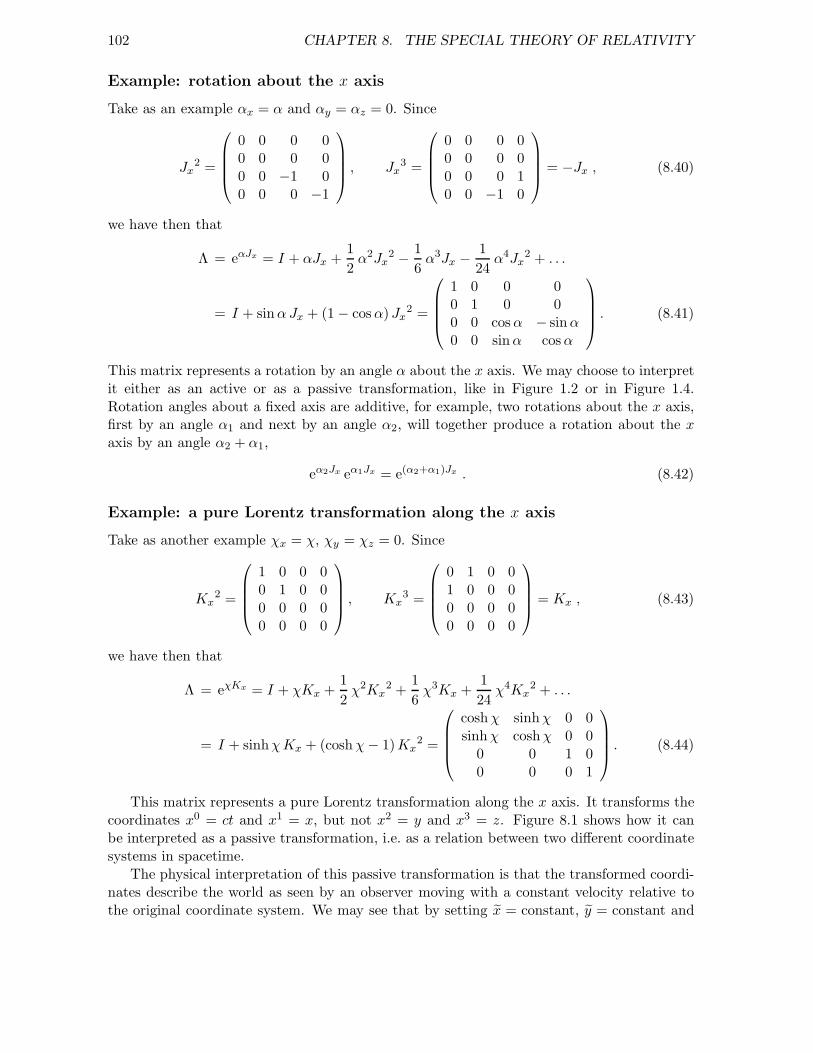
102 CHAPTER 8. THE SPECIAL THEORY OF RELATIVITY
Example: rotation about the x axis
Take as an example αx = α and αy = αz = 0. Since
Jx2 =
0 0 0 00 0 0 00 0 −1 00 0 0 −1
, Jx
3 =
0 0 0 00 0 0 00 0 0 10 0 −1 0
= −Jx , (8.40)
we have then that
Λ = eαJx = I + αJx +1
2α2Jx
2 − 1
6α3Jx − 1
24α4Jx
2 + . . .
= I + sinαJx + (1 − cosα)Jx2 =
1 0 0 00 1 0 00 0 cosα − sinα0 0 sinα cosα
. (8.41)
This matrix represents a rotation by an angle α about the x axis. We may choose to interpretit either as an active or as a passive transformation, like in Figure 1.2 or in Figure 1.4.Rotation angles about a fixed axis are additive, for example, two rotations about the x axis,first by an angle α1 and next by an angle α2, will together produce a rotation about the xaxis by an angle α2 + α1,
eα2Jx eα1Jx = e(α2+α1)Jx . (8.42)
Example: a pure Lorentz transformation along the x axis
Take as another example χx = χ, χy = χz = 0. Since
Kx2 =
1 0 0 00 1 0 00 0 0 00 0 0 0
, Kx
3 =
0 1 0 01 0 0 00 0 0 00 0 0 0
= Kx , (8.43)
we have then that
Λ = eχKx = I + χKx +1
2χ2Kx
2 +1
6χ3Kx +
1
24χ4Kx
2 + . . .
= I + sinhχKx + (coshχ− 1)Kx2 =
coshχ sinhχ 0 0sinhχ coshχ 0 0
0 0 1 00 0 0 1
. (8.44)
This matrix represents a pure Lorentz transformation along the x axis. It transforms thecoordinates x0 = ct and x1 = x, but not x2 = y and x3 = z. Figure 8.1 shows how it canbe interpreted as a passive transformation, i.e. as a relation between two different coordinatesystems in spacetime.
The physical interpretation of this passive transformation is that the transformed coordi-nates describe the world as seen by an observer moving with a constant velocity relative tothe original coordinate system. We may see that by setting x = constant, y = constant and
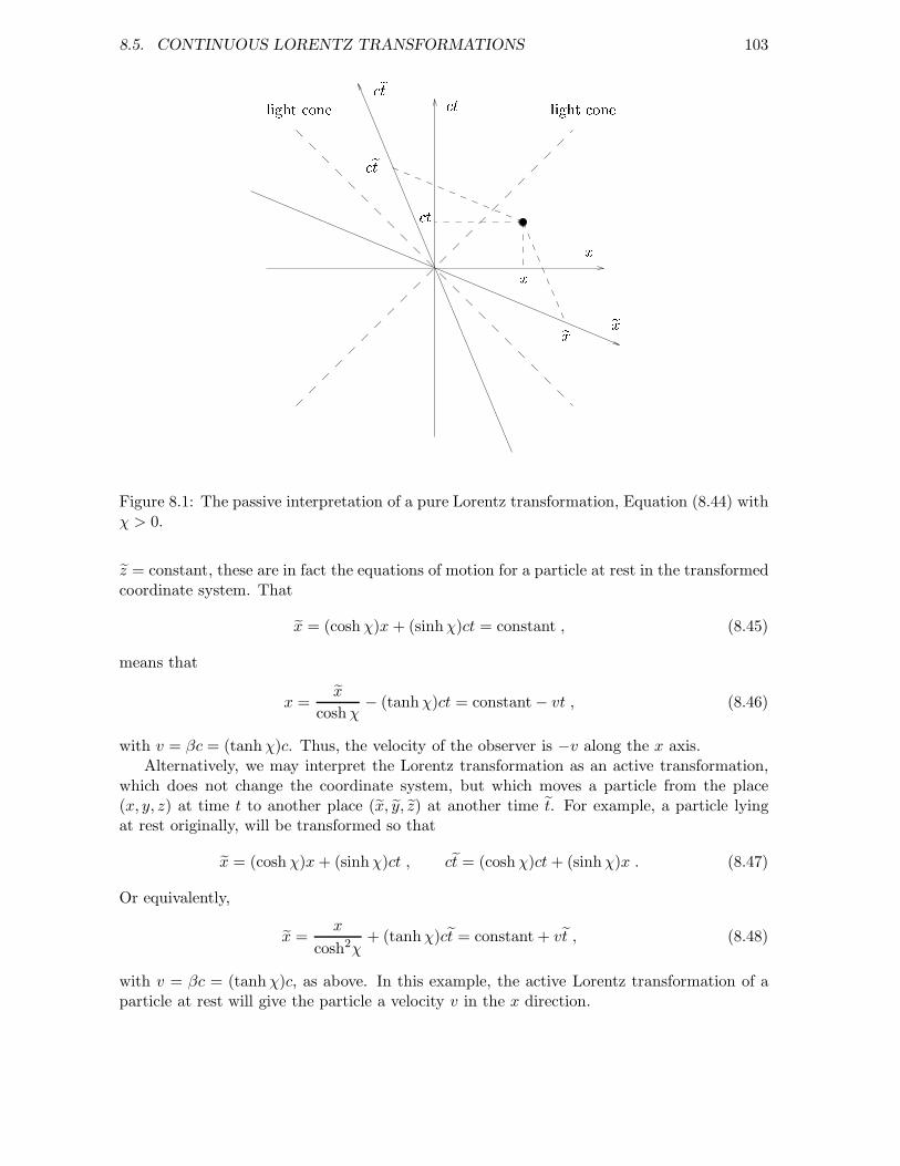
8.5. CONTINUOUS LORENTZ TRANSFORMATIONS 103
x tlight onelight one
exx t et et
exFigure 8.1: The passive interpretation of a pure Lorentz transformation, Equation (8.44) withχ > 0.
z = constant, these are in fact the equations of motion for a particle at rest in the transformedcoordinate system. That
x = (coshχ)x+ (sinhχ)ct = constant , (8.45)
means that
x =x
coshχ− (tanhχ)ct = constant − vt , (8.46)
with v = βc = (tanhχ)c. Thus, the velocity of the observer is −v along the x axis.Alternatively, we may interpret the Lorentz transformation as an active transformation,
which does not change the coordinate system, but which moves a particle from the place(x, y, z) at time t to another place (x, y, z) at another time t. For example, a particle lyingat rest originally, will be transformed so that
x = (coshχ)x+ (sinhχ)ct , ct = (coshχ)ct+ (sinhχ)x . (8.47)
Or equivalently,
x =x
cosh2χ+ (tanhχ)ct = constant + vt , (8.48)
with v = βc = (tanhχ)c, as above. In this example, the active Lorentz transformation of aparticle at rest will give the particle a velocity v in the x direction.
104 CHAPTER 8. THE SPECIAL THEORY OF RELATIVITY
The parameter χ is called rapidity. It is additive, in the same way as the rotation angleabout a fixed axis. As we have seen, the relation between the rapidity χ and the velocityv = βc is that
β = tanhχ =sinhχ
coshχ=
eχ − e−χ
eχ + e−χ, (8.49)
which is the same as
eχ =
√1 + β
1 − β. (8.50)
By defining
γ =1√
1 − β2= coshχ , (8.51)
we may write
Λ =
γ γβ 0 0γβ γ 0 00 0 1 00 0 0 1
. (8.52)
The Lie algebra of the Lorentz group
The group multiplication in the proper Lorentz group, which is the connection componentof the Lorentz group containing the identity transformation I but not the discrete trans-formations P , T and PT , is given by the Lie algebra. In other words, the compositionof proper Lorentz transformations is given by the commutation relations of the generatorsJ = (Jx, Jy , Jz) and K = (Kx,Ky,Kz),
[Jx, Jy] = −[Kx,Ky] = Jz , [Jx,Ky] = [Kx, Jy] = Kz ,
[Jy, Jz] = −[Ky,Kz] = Jx , [Jy,Kz] = [Ky, Jz ] = Kx , (8.53)
[Jz , Jx] = −[Kz,Kx] = Jy , [Jz,Kx] = [Kz, Jx] = Ky ,
[Jx,Kx] = [Jy,Ky] = [Jz,Kz ] = 0 . (8.54)
The same commutation relations may be expressed more compactly in terms of the com-plex matrices
M±k =
1
2(Jk ± iKk) . (8.55)
We see that [M+j ,M
−k ] = 0 for j, k = x, y, z, and that
[M+x ,M
+y ] = M+
z , [M+y ,M
+z ] = M+
x , [M+z ,M
+x ] = M+
y ,
[M−x ,M
−y ] = M−
z , [M−y ,M
−z ] = M−
x , [M−z ,M
−x ] = M−
y . (8.56)
8.6. THE LAW OF COSMIC LAZINESS 105
The full Lorentz group
In order to complete the multiplication table of the Lorentz group, we have to include thefollowing relations involving the discrete transformations P , T and PT = TP ,
P 2 = T 2 = (PT )2 = I , (8.57)
and
PJ = JP , TJ = JT , PK = −KP , TK = −KT . (8.58)
The last relations imply e.g. that
P (α · J + χ · K)2 = (α · J − χ · K)P (α · J + χ · K) = (α · J − χ · K)2 P . (8.59)
More generally, P (α · J + χ · K)n = (α · J − χ · K)n P when n ≥ 0, and
P eα·J+χ·K = eα·J−χ·K P , T eα·J+χ·K = eα·J−χ·K T . (8.60)
8.6 The law of cosmic laziness
A point particle not influenced by external forces will move in a straight line with constantvelocity. This is a basic postulate of the special theory of relativity, and it serves both as adefintion of the inertial frames that are the privileged coordinate systems, and as a law ofmotion.
A remarkable property of the inertial motion of a particle, according to the special theoryof relativity, is that it maximizes the proper time τ , which is the time measured by a clockfollowing the motion. This property may be used as a variational principle determining theequation of motion. Bertrand Russell gave this principle a highly appropriate name, callingit the law of cosmic laziness.
The effect that the proper time τ differs from the coordinate time t measured in an inertialsystem, is called time dilatation. The relation between τ and t is that
dτ = dt
√
1 − v2
c2, (8.61)
for a particle moving with velocity
v =dr
dt. (8.62)
The time dilatation is experimentally verified both with an atomic clock that was flownaround the Earth, and by comparison of the lifetimes of unstable particles moving withdifferent velocities, from zero velocity up to velocities extremely close to the speed of light.
Instead of the proper time τ we may introduce the “relativistic length” s = cτ , defined ingeneral by the relation
ds2 = c2 dτ2 = c2 dt2 − |dr|2 = gµνdxµ dxν . (8.63)
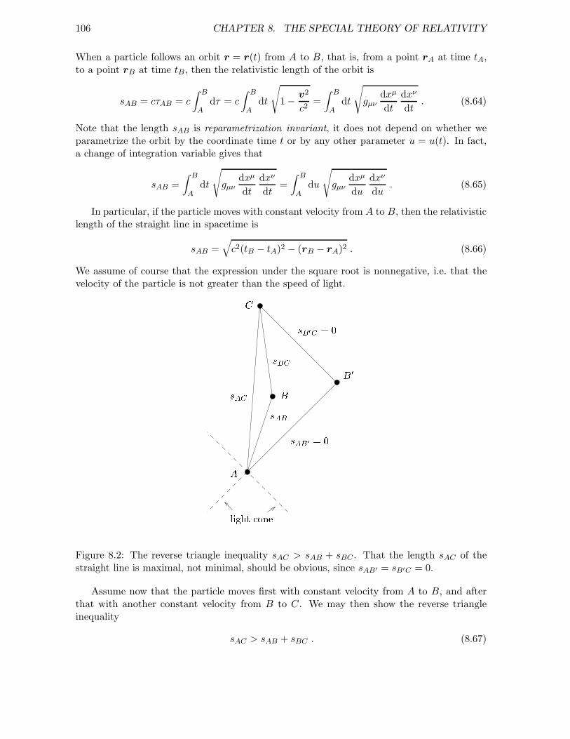
106 CHAPTER 8. THE SPECIAL THEORY OF RELATIVITY
When a particle follows an orbit r = r(t) from A to B, that is, from a point rA at time tA,to a point rB at time tB , then the relativistic length of the orbit is
sAB = cτAB = c
∫ B
Adτ = c
∫ B
Adt
√
1 − v2
c2=
∫ B
Adt
√
gµνdxµ
dt
dxν
dt. (8.64)
Note that the length sAB is reparametrization invariant, it does not depend on whether weparametrize the orbit by the coordinate time t or by any other parameter u = u(t). In fact,a change of integration variable gives that
sAB =
∫ B
Adt
√
gµνdxµ
dt
dxν
dt=
∫ B
Adu
√
gµνdxµ
du
dxν
du. (8.65)
In particular, if the particle moves with constant velocity from A to B, then the relativisticlength of the straight line in spacetime is
sAB =√c2(tB − tA)2 − (rB − rA)2 . (8.66)
We assume of course that the expression under the square root is nonnegative, i.e. that thevelocity of the particle is not greater than the speed of light.
BsBC
light one
CsAB sAB0 = 0
sB0C = 0 B0sACA
Figure 8.2: The reverse triangle inequality sAC > sAB + sBC . That the length sAC of thestraight line is maximal, not minimal, should be obvious, since sAB′ = sB′C = 0.
Assume now that the particle moves first with constant velocity from A to B, and afterthat with another constant velocity from B to C. We may then show the reverse triangleinequality
sAC > sAB + sBC . (8.67)
8.7. LORENTZ CONTRACTION 107
See Figure 8.2. The inversion of the inequality sign compared to what we are used to fromEuclidean geometry is due to the minus signs under the square root sign in Equation (8.66).An extreme example is the triangle AB′C in Figure 8.2, where two sides have zero length,because they represent light signals.
The simplest way to prove Equation (8.67) is to use the Lorentz invariance of the rela-tivistic length s, implying that it is sufficient to prove the special case rA = rC 6= rB. In thiscase we see directly that
sAC = c(tC − tA) = c(tB − tA) + c(tC − tB) > sAB + sBC . (8.68)
We may use the reverse triangle inequality for an arbitrary orbit, which we divide intosmall or infinitesimal pieces. We realize that by straightening out the orbit we will increaseits length, which is c times the proper time along the orbit. Thus, the general conclusion isthat when a particle moves in a straight line with constant velocity, this is the motion thatmakes the proper time τ maximal.
The twin paradox
The famous so called twin paradox is nothing but the reverse triangle inequality in termsof the proper time τ = s/c. The effect is that an astronaut travelling far out in space witha high velocity, then turning around and returning, will be younger on his return than histwin who remained stationary. What may seem paradoxical is the asymmetry of the effect.Both twins see the other one moving away and coming back, but when they meet again, onewill definitely be older and the other one younger. There should be no paradox here, oncewe realize that the one who will be oldest, is the one who has followed a straight line, alsocalled a geodesic path, in spacetime. The twin paradox is really no more paradoxical than thefact that a straight line in Euclidean space is shorter than any other curve joining two givenpoints.
8.7 Lorentz contraction
Two observers A and B moving with a constant velocity v = βc relative to each other maychoose their x, y and z axes such that the transformation between the two coordinate systemsis a pure Lorentz transformation in the x direction, as in Equation (8.52).
Imagine now a measuring rod of length L lying at rest relative to the observer B andmoving relative to A with a velocity v = βc in the negative x direction. We ask how long theobserver A will measure the rod to be.
Since the transversal coordinates y and z are unchanged by the transformation, we predictthat A will measure the same length L if the rod is oriented in the transversal direction. Thisconclusion is also the only one possible, based on the principle of relativity, that there shouldbe a complete symmetry between the two observers.
In fact, A may in principle measure the length of the moving rod by arranging for thetwo ends of the rod to make scratch marks at the moment when the rod passes by. But inthe same way, the stationary measuring rod used by A, of length L and transversely oriented,may in principle produce scratch marks on the moving rod. By such experiments the twoobservers will observe the same unambiguous fact, either that the two rods are equally long,or that one of them is shorter than the other one. But the rod which is moving relative to
108 CHAPTER 8. THE SPECIAL THEORY OF RELATIVITY
observer A is stationary relative to B, and vice versa. Hence the only result consistent withthe symmetry between the two observers, is that the measured lengths are equal.
If the measuring rod moving relative to A is oriented in the x direction, parallel to thevelocity, then the situation is different. The observer B sees the two ends of the rod lying atrest, with constant x coordinates xa and xb. According to the Lorentz transformation,
xa = γ(xa + vta) , xb = γ(xb + vtb) , (8.69)
with the obvious notation. Thus, if the observer A looks where the two ends are located atone given time ta = tb, then we have
L = xb − xa = γ(xb − xa + v(tb − ta)) = γ(xb − xa) . (8.70)
Thus, A observes a distance between the two end points which is
LA = xb − xa =L
γ= L
√
1 − v2
c2. (8.71)
Using this particular measuring procedure, A finds a length shorter than L. This contractionof the length of a moving object in the direction of motion is called Lorentz contraction. Thatit is a real physical effect, like the time dilatation, and not just an illusion, is illustrated bythe thought experiment described in Problem 8.
8.8 Addition of velocities, constant acceleration
When adding velocities in the theory of relativity, it seems that we have to modify the standardrules for addition. In particular, whatever velocity we add to that of a light signal, the summust always be the velocity of light. The light from a lamp moves with the velocity c relativeto the lamp, but even if the lamp moves with velocity v in the same direction as it is shining,the velocity of the light is still c and not c + v. Thus, for velocities in a fixed direction, theunorthodox rule c + v = c must hold. The speed of light is the ultimate speed limit, it cannever be exceeded no matter how much we add velocities.
The general formula for the addition of velocities in the x direction is derived from theLorentz transformation. Assume that A moves with velocity u relative to B, and that Bmoves with velocity v relative to C. Then B sees A moving a distance ∆x = u∆t during asmall time interval ∆t, whereas C observes A moving a distance
∆x = γ(∆x+ βc∆t) (8.72)
during the time interval
∆t = γ
(∆t+ β
∆x
c
). (8.73)
Here we have
β =v
c, γ =
1√1 − β2
. (8.74)
8.8. ADDITION OF VELOCITIES, CONSTANT ACCELERATION 109
Thus, C sees A moving with the velocity
w =∆x
∆t=
∆x+ βc∆t
∆t+ β ∆xc
=u+ v
1 + uvc2
. (8.75)
It follows from this formula that the rapidity is additive, instead of the velocity. Introducingthe rapidities χ1 and χ2 such that u = c tanhχ1 and v = c tanhχ2, we get that
w =u+ v
1 + uvc2
=c(tanhχ1 + tanhχ2)
1 + (tanhχ1)(tanhχ2)= c tanh(χ1 + χ2) . (8.76)
We may use the velocity addition formula to find the motion of a particle acceleratingwith a constant acceleration a. The reasonable way to define constant acceleration is thatthe particle itself at any time feels an acceleration equal to a constant value a. Thus, theacceleration should be a in the instantaneous rest system, which is an inertial reference systemin which the particle lies at rest at the given moment.
Let τ denote the proper time of the particle, defined such that the particle is at rest atthe proper time τ = 0. As seen from the instantaneous rest system, the particle increasesits velocity from zero to adτ during the infinitesimal time interval dτ . Thereby it jumps ofcourse into another rest system, but let us stay in the same inertial frame. As seen from thereference system in which the particle was initially at rest, at τ = 0, the velocity increases inthe proper time interval dτ from v to
v + dv =v + adτ
1 + vadτc2
= (v + adτ)
(1 − vadτ
c2
)= v + adτ
(1 − v2
c2
). (8.77)
We may write this equation as
adτ =c2 dv
c2 − v2=
dv
2
(c
c+ v+
c
c− v
). (8.78)
Integration gives that
aτ = c ln
√c+ v
c− v. (8.79)
Or equivalently,
v = c tanh
(aτ
c
). (8.80)
We see that constant acceleration in the theory of relativity means that the rapidityχ = arctanh(v/c) increases linearly with the proper time τ .
The relation between the proper time τ and the time t in a fixed reference system is that
dt =dτ√
1 − v2
c2
= dτ cosh
(aτ
c
). (8.81)
Defining t = 0 at τ = 0, we get that
t =c
asinh
(aτ
c
), (8.82)

110 CHAPTER 8. THE SPECIAL THEORY OF RELATIVITY
and hence,
v =at√
1 +(at)2
c2
. (8.83)
Let us choose the coordinate system such that x = 0 at t = 0, then integration of the equationdx/dt = v gives that
x =c2
a
√
1 +(at)2
c2− 1
=
c2
a
(cosh
(aτ
c
)− 1
). (8.84)
Note that with a > 0, the particle moves in such a way that the following inequalityalways holds,
x > ct− c2
a. (8.85)
Even though it is impossible for anything other than light (plus gravitational waves and maybeneutrinos) to reach the speed of light, it is theoretically possible to outrun a light signal, ifone can get a sufficient head start and run with a constant acceleration.
One consequence of this startling fact is that a runner with constant acceleration a > 0along the x axis runs in front of a horizon moving with the speed of light. If the runner startsat x = 0 at time t = 0, the position of the horizon at time t is
x = ct− c2
a. (8.86)
This is a horizon because it is impossible for the runner to see past it. The runner can neverget any information about any event taking place along the x axis at the place x′ at the timet′, if x′ < ct′ − (c2/a).
8.9 Relativistic conservation laws
Any relativistic conservation law must necessarily be local, because it must hold in all inertialframes, and because simultaneity is a relative concept. For example, energy conservation inall inertial frames does not allow one joule of energy to move instantaneously from one placeA to another place B, one kilometer away. The two events, the energy disappearing at Aand reappearing at B, would not look simultaneous to all observers. Some observers wouldsee energy not conserved, because they would see it appearing at B either before or after itdisappeared at A. Because charge and energy are locally conserved quantities, they have tobe carried along through a cable from the power station to the light bulb.
Consider the conservation of electric charge as a concrete example, illustrated in Figure 8.3.The charge inside a three dimensional region Ω3 at time t is the integral over Ω3 of the chargedensity ρ = ρ(r, t),
q(t) =
∫
Ω3
d3r ρ(r, t) . (8.87)
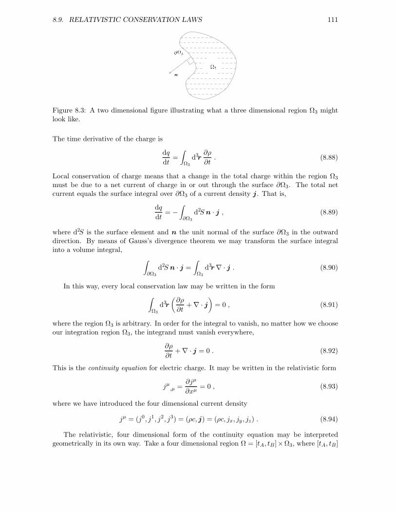
8.9. RELATIVISTIC CONSERVATION LAWS 111n@3 3Figure 8.3: A two dimensional figure illustrating what a three dimensional region Ω3 mightlook like.
The time derivative of the charge is
dq
dt=
∫
Ω3
d3r∂ρ
∂t. (8.88)
Local conservation of charge means that a change in the total charge within the region Ω3
must be due to a net current of charge in or out through the surface ∂Ω3. The total netcurrent equals the surface integral over ∂Ω3 of a current density j. That is,
dq
dt= −
∫
∂Ω3
d2S n · j , (8.89)
where d2S is the surface element and n the unit normal of the surface ∂Ω3 in the outwarddirection. By means of Gauss’s divergence theorem we may transform the surface integralinto a volume integral,
∫
∂Ω3
d2S n · j =
∫
Ω3
d3r∇ · j . (8.90)
In this way, every local conservation law may be written in the form
∫
Ω3
d3r
(∂ρ
∂t+ ∇ · j
)= 0 , (8.91)
where the region Ω3 is arbitrary. In order for the integral to vanish, no matter how we chooseour integration region Ω3, the integrand must vanish everywhere,
∂ρ
∂t+ ∇ · j = 0 . (8.92)
This is the continuity equation for electric charge. It may be written in the relativistic form
jµ,µ =∂jµ
∂xµ= 0 , (8.93)
where we have introduced the four dimensional current density
jµ = (j0, j1, j2, j3) = (ρc, j) = (ρc, jx, jy , jz) . (8.94)
The relativistic, four dimensional form of the continuity equation may be interpretedgeometrically in its own way. Take a four dimensional region Ω = [tA, tB ]×Ω3, where [tA, tB ]
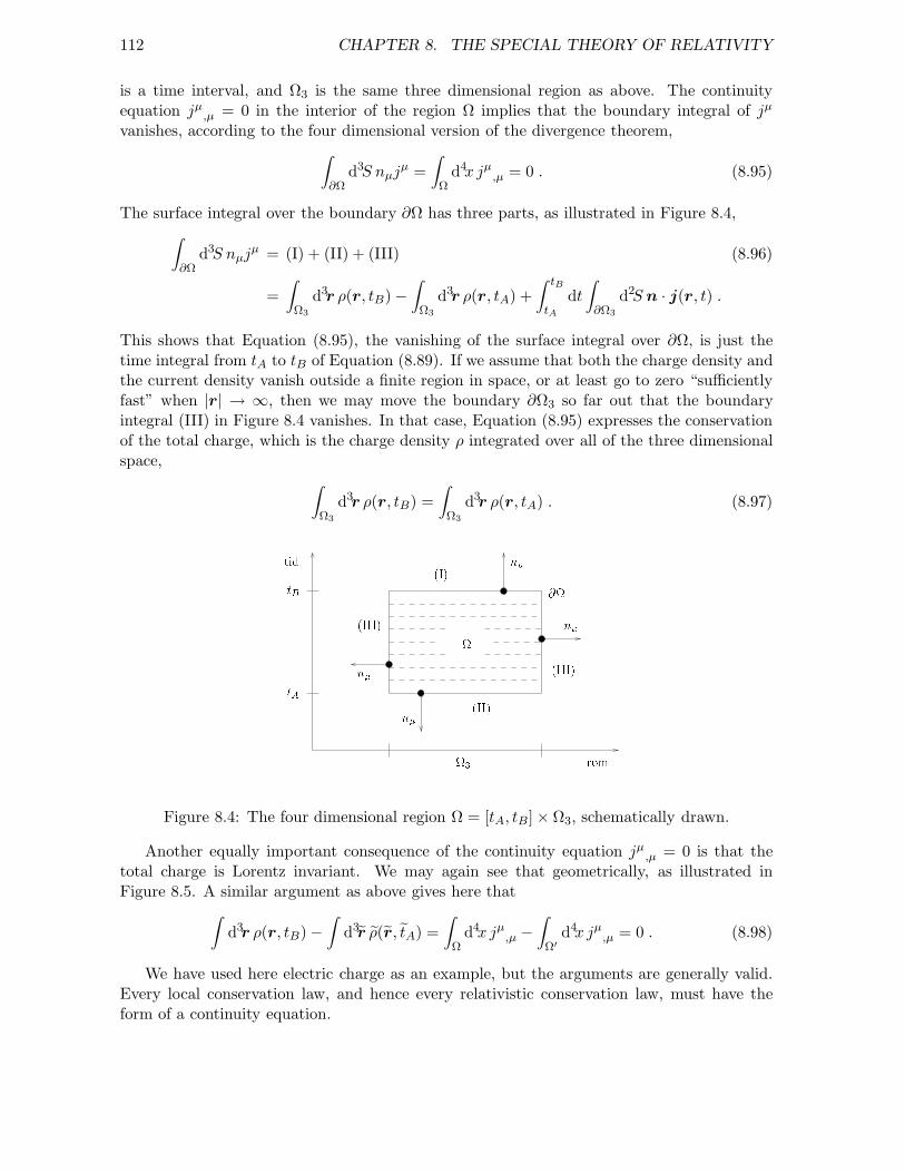
112 CHAPTER 8. THE SPECIAL THEORY OF RELATIVITY
is a time interval, and Ω3 is the same three dimensional region as above. The continuityequation jµ,µ = 0 in the interior of the region Ω implies that the boundary integral of jµ
vanishes, according to the four dimensional version of the divergence theorem,
∫
∂Ωd3S nµj
µ =
∫
Ωd4x jµ,µ = 0 . (8.95)
The surface integral over the boundary ∂Ω has three parts, as illustrated in Figure 8.4,
∫
∂Ωd3S nµj
µ = (I) + (II) + (III) (8.96)
=
∫
Ω3
d3r ρ(r, tB) −∫
Ω3
d3r ρ(r, tA) +
∫ tB
tA
dt
∫
∂Ω3
d2S n · j(r, t) .
This shows that Equation (8.95), the vanishing of the surface integral over ∂Ω, is just thetime integral from tA to tB of Equation (8.89). If we assume that both the charge density andthe current density vanish outside a finite region in space, or at least go to zero “sufficientlyfast” when |r| → ∞, then we may move the boundary ∂Ω3 so far out that the boundaryintegral (III) in Figure 8.4 vanishes. In that case, Equation (8.95) expresses the conservationof the total charge, which is the charge density ρ integrated over all of the three dimensionalspace,
∫
Ω3
d3r ρ(r, tB) =
∫
Ω3
d3r ρ(r, tA) . (8.97)@ntid nn (III)(II)(III) n(I)
romtAtB 3Figure 8.4: The four dimensional region Ω = [tA, tB] × Ω3, schematically drawn.
Another equally important consequence of the continuity equation jµ,µ = 0 is that thetotal charge is Lorentz invariant. We may again see that geometrically, as illustrated inFigure 8.5. A similar argument as above gives here that
∫d3r ρ(r, tB) −
∫d3r ρ(r, tA) =
∫
Ωd4x jµ,µ −
∫
Ω′
d4x jµ,µ = 0 . (8.98)
We have used here electric charge as an example, but the arguments are generally valid.Every local conservation law, and hence every relativistic conservation law, must have theform of a continuity equation.
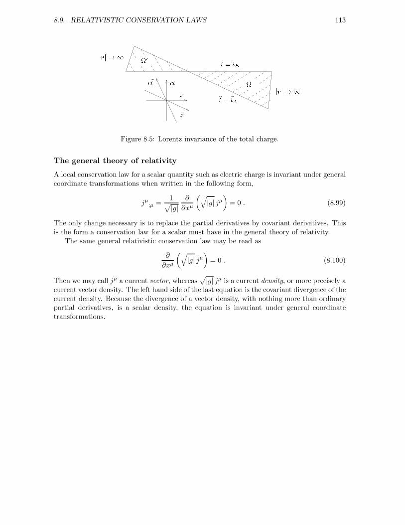
8.9. RELATIVISTIC CONSERVATION LAWS 113xct jrj ! 1t = tBcet ex et = etAjrj ! 1 0 Figure 8.5: Lorentz invariance of the total charge.
The general theory of relativity
A local conservation law for a scalar quantity such as electric charge is invariant under generalcoordinate transformations when written in the following form,
jµ;µ =1√|g|
∂
∂xµ
(√|g| jµ
)= 0 . (8.99)
The only change necessary is to replace the partial derivatives by covariant derivatives. Thisis the form a conservation law for a scalar must have in the general theory of relativity.
The same general relativistic conservation law may be read as
∂
∂xµ
(√|g| jµ
)= 0 . (8.100)
Then we may call jµ a current vector, whereas√|g| jµ is a current density, or more precisely a
current vector density. The left hand side of the last equation is the covariant divergence of thecurrent density. Because the divergence of a vector density, with nothing more than ordinarypartial derivatives, is a scalar density, the equation is invariant under general coordinatetransformations.

114 CHAPTER 8. THE SPECIAL THEORY OF RELATIVITY
Problems
1. Find the 4 × 4 matrices describing:
a) rotation by a given angle about the y axis;
b) rotation about the z axis;
c) a pure Lorentz transformation along the y axis;
d) a pure Lorentz transformation along the z axis;
e) a rotation about the x axis, followed by a pure Lorentz transformation along they axis;
f) a pure Lorentz transformation along the y axis, followed by a rotation about thex axis.
2. Compute the matrix eα(Jx+Ky), representing a somewhat special Lorentz transformationwhich is a combination of a rotation and a pure Lorentz transformation.Show explicitly that this is a Lorentz transformation, i.e. preserves the metric ηµν .Show that it leaves the null vector Aµ = (1, 0, 0, 1) invariant.We call Aµ a null (or lightlike) vector because ηµνA
µAν = 0.
3. Derive the formula for time dilatation, Equation (8.61).
4. The distance to Sirius, one of the closest stars, is 9 light years. How long time does around trip to Sirius and back take with a velocity of 180 000 km/s (0.6 c), if we disregardthe time it takes to accelerate to this velocity and to brake down again? To be moreprecise, how long time does it take for those who travel, and for those who wave goodbyeand sit at home waiting for the astronauts to return?Is it a realistic project to travel through space at a velocity of 0.6 c? In fact, even the“empty” interstellar space is not quite empty, but contains a certain amount of gas,dust and radiation.
5. Is it realistic to neglect the acceleration and deceleration periods in the previous prob-lem? In other words, how long time (coordinate time and proper time) does it taketo accelerate up to a velocity of 180 000 km/s, with an acceleration of 10 m/s2? Theacceleration should be measured relative to the instantaneous rest system, in which theaccelerated object is momentarily at rest.The acceleration of gravity on the surface of the Earth, g = 9, 81 m/s2, is roughly themaximum acceleration that the human body can support.
6. How much energy is needed (at least) to accelerate a space ship with a mass of 105 kgup to 180 000 km/s? The relativistic formula for the energy of a particle of mass (i.e.rest mass) m and velocity v is
E =mc2√1 − v2
c2
.
In order to find a lower bound to the energy needed, we may neglect any details of theacceleration process. If such a project should ever become a reality, the accelerationwould presumably be provided by a rocket engine working over an extended period of
8.9. RELATIVISTIC CONSERVATION LAWS 115
time. This would presumably cost much more than the minimum amount of energy,because the rocket engine at any time would have to accelerate also the remaining rocketfuel. It turns out that the efficiency of a rocket engine depends very much on the speedof its exhaust gas.
7. If an astronaut starts on his (or her) 30th birthday, and accelerates all the time in thesame direction with a constant acceleration of 10 m/s2, how far away will he (she) beon his (her) 40th birthday? 50th birthday? 60th birthday?
8. Two space ships lie at rest one kilometer away from each other, and are connected by arope which is pulled tight but not stressed. They start simultaneously to accelerate inthe same direction. One space ship accelerates in the direction away from the second,which follows behind on the same course. Both accelerate by 10 m/s2, until reaching avelocity of exactly 0.6 c relative to the original rest system. Then they stop acceleratingand move on at constant velocity.What will happen to the rope connecting them?This is a famous thought experiment, rather more paradoxical than the twin paradox.
116 CHAPTER 8. THE SPECIAL THEORY OF RELATIVITY
Chapter 9
Particle mechanics
The basic idea of the Lagrange and Hamilton formalism is to derive the equations of motiondescribing a physical system from a variational principle. This turns out to be a very powerfulmethod, in particle mechanics as in field theory, both classical and quantum. One obviousreason is that the variational principle is a very compact formulation of the equations of mo-tion. Furthermore, it usually exhibits very clearly the symmetries of the theory, and throughNoether’s theorem it gives a fundamental relation between symmetries and conservation laws.
We consider in this chapter mechanical systems with a finite number of degrees of freedom,typically systems consisting of idealized point particles. The equations of motion, in the formin which they are usually solved, are then ordinary differential equations for the particlecoordinates as functions of time t.
9.1 Newton’s second law
The basic equation in classical mechanics is Newton’s second law for a non-relativistic pointparticle,
F = ma . (9.1)
Here F is the force acting on the particle, and the mass m is a proportionality constantcharacteristic of the particle. The position of the particle is a function of time, r = r(t), andthe velocity v and acceleration a are the time derivatives of the position,
v =dr
dt, a =
dv
dt=
d2r
dt2. (9.2)
Newton’s second law, written in the form
d2r
dt2=
F
m, (9.3)
is an equation of motion that may be integrated to give the position r(t) at any time t if weknow the position r(t0) and velocity v(t0) at a given time t0, and if we also know the forceF acting on the particle at all times.
Newton’s second law belongs to classical physics and does not apply to a quantum me-chanical system like the electron in the hydrogen atom. On the other hand, it holds in a
117
118 CHAPTER 9. PARTICLE MECHANICS
suitably modified form even if the particle is relativistic, moving with a velocity approachingthe speed of light. For example, the classical relativistic equation of motion applies to elec-trons and protons in particle accelerators, where the electrons may reach velocities so closeto the speed of light that they lose less than a centimeter per second. We will return to therelativistic generalization of Newton’s second law at the end of the next chapter.
The force F acting on a particle will usually vary along the orbit of the particle. Thework performed by the force, from one point A at time tA to another point B at time tB , is
WAB =
∫ tB
tA
dt v · F =
∫ B
Adr · F . (9.4)
This work changes the kinetic energy of the particle, defined as
EK =1
2mv2 . (9.5)
In fact, it follows from Newton’s second law that
WAB =
∫ tB
tA
dt v · (ma) =1
2m
∫ tB
tA
dtdv2
dt=
1
2mvB
2 − 1
2mvA
2 . (9.6)
In many cases of interest the particle is moving in a force field, for example a gravitationalfield or an electromagnetic field, where the force is minus the gradient of a potential energyfunction,
F = −∇V , (9.7)
at the point where the particle is located. The potential energy V = V (r, t) is a function ofthe position r and the time t. In an electromagnetic field we may need to introduce also avelocity dependence in the potential energy, as we will see below.
When the potential energy is not explicitly time dependent, i.e. V = V (r), then thesystem is said to be conservative, because the total energy E = EK + V of the particle, thesum of its kinetic and potential energy, is conserved. In fact, we have that
dE
dt=
d
dt
(1
2mv2 + V
)= mv · a + (∇V ) · v = (ma + ∇V ) · v = 0 . (9.8)
In this case we have, at least in principle, a clear procedure for measuring the potential energyV , or more precisely the difference in potential energy from one point rA to another pointrB . We may move the particle from rA to rB along any prescribed path r = r(t) by applyingan external force F 1 chosen such that
F 1 −∇V = md2r
dt2. (9.9)
First we keep the particle at rest at rA, so that it has no kinetic energy. Next we move it torB , where we again keep it at rest so that it has no kinetic energy. Since the kinetic energyis zero to begin with and zero at the end of the whole process, the total work done on theparticle is zero,
0 =
∫ B
Adr · F =
∫ B
Adr · (F 1 −∇V ) . (9.10)
9.2. HAMILTON’S PRINCIPLE 119
Or equivalently,
∫ B
Adr · F 1 =
∫ B
Adr · (∇V ) =
∫ B
AdV = V (rB) − V (rA) . (9.11)
The line integral of the external force F 1 is measurable. We see that it is independent of thepath along which the particle is moved, it depends only on the end points rA and rB of thepath, and it is equal to the difference in potential energy between the two points.
9.2 Hamilton’s principle
From the example of one particle in three dimensions we generalize to a classical mechanicalsystem with d degrees of freedom, i.e. a system described by d coordinates xi, with i =1, 2, . . . , d. We call them generalized coordinates, because we need not choose them as thestandard Eucliden coordinates, we may use polar coordinates instead, or any other coordinatessuitable for the system we study. The coordinates need not have the physical dimension oflength, or even the same dimension. The Lagrange and Hamilton formalism makes it easyto change coordinates, and this is one of its great advantages, especially when we wantto formulate equations of motion that are generally covariant, i.e. invariant under generalcoordinate transformations.
To simplify the notation, we often do not write the coordinate index i, but write x for allcoordinates simultaneously,
x = (x1, x2, . . . , xd) . (9.12)
In other words, x denotes a point in a d-dimensional configuration space.The motion of the system follows an orbit such that the position, or configuration, at time
t is x = x(t). The velocity is the time derivative of the position,
x = (x1, x2, . . . , xd) , with xi =dxi
dt. (9.13)
Thus, our notation is ambiguous in that the same symbol x may denote either a single pointin the configuration space, or a complete time dependent orbit.
The Lagrange function for a non-relativistic system is usually the difference between thekinetic energy EK and the potential energy V ,
L = EK − V . (9.14)
The Lagrange function for a system of relativistic particles has a different form. In whatfollows, we will allow L to have a quite general dependence on position and velocity,
L = L(x, x, t) = L(x1, x2, . . . , xd, x1, x2, . . . , xd, t) . (9.15)
Note that L is an implicit function of time t, since x = x(t) and x = x(t), but we allow alsofor the possibility that L may depend explicitly on t. Below we will consider briefly the moregeneral case when L depends on the acceleration x, i.e. L = L(x, x, x, t). We never include inthe Lagrange function higher than second order time derivatives.
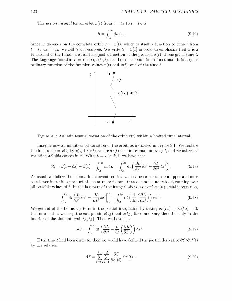
120 CHAPTER 9. PARTICLE MECHANICS
The action integral for an orbit x(t) from t = tA to t = tB is
S =
∫ tB
tA
dt L . (9.16)
Since S depends on the complete orbit x = x(t), which is itself a function of time t fromt = tA to t = tB, we call S a functional. We write S = S[x] in order to emphasize that S is afunctional of the function x, and not just a function of the position x(t) at one given time t.The Lagrange function L = L(x(t), x(t), t), on the other hand, is no functional, it is a quiteordinary function of the function values x(t) and x(t), and of the time t.x(t)x(t) + x(t)B
A xt
Figure 9.1: An infinitesimal variation of the orbit x(t) within a limited time interval.
Imagine now an infinitesimal variation of the orbit, as indicated in Figure 9.1. We replacethe function x = x(t) by x(t)+ δx(t), where δx(t) is infinitesimal for every t, and we ask whatvariation δS this causes in S. With L = L(x, x, t) we have that
δS = S[x+ δx] − S[x] =
∫ tB
tA
dt δL =
∫ tB
tA
dt
(∂L
∂xiδxi +
∂L
∂xiδxi). (9.17)
As usual, we follow the summation convention that when i occurs once as an upper and onceas a lower index in a product of one or more factors, then a sum is understood, running overall possible values of i. In the last part of the integral above we perform a partial integration,
∫ tB
tA
dt∂L
∂xiδxi =
∂L
∂xiδxi
∣∣∣∣tB
tA
−∫ tB
tA
dt
(d
dt
(∂L
∂xi
))δxi . (9.18)
We get rid of the boundary term in the partial integration by taking δx(tA) = δx(tB) = 0,this means that we keep the end points x(tA) and x(tB) fixed and vary the orbit only in theinterior of the time interval [tA, tB ]. Then we have that
δS =
∫ tB
tA
dt
(∂L
∂xi− d
dt
(∂L
∂xi
))δxi . (9.19)
If the time t had been discrete, then we would have defined the partial derivative ∂S/∂xi(t)by the relation
δS =tB∑
t=tA
d∑
i=1
∂S
∂xi(t)δxi(t) . (9.20)
9.2. HAMILTON’S PRINCIPLE 121
When t is a continuous variable, so that the sum over t has to be replaced by an integral,then we define the functional derivative δS/δxi(t) by the relation
δS =
∫ tB
tA
dtd∑
i=1
δS
δxi(t)δxi(t) . (9.21)
This definition gives that
δS
δxi=∂L
∂xi− d
dt
(∂L
∂xi
). (9.22)
The equation of motion for the system may be derived from the action integral by meansof
Hamilton’s principle. The motion of the system from position x(tA) at timetA to position x(tB) at time tB follows an orbit x(t) such that the action integralS is extremal. That is,
δS = 0 (9.23)
for every infinitesimal variation δx(t) from the orbit x(t) such that δx(tA) =δx(tB) = 0.
The equation of motion derived from Hamilton’s principle is the Euler–Lagrange equation,
δS
δxi=∂L
∂xi− d
dt
(∂L
∂xi
)= 0 . (9.24)
It consists of d equations at every value of t, one equation for each coordinate xi(t) which isvaried.
In order to prove that the Euler–Lagrange equation follows from Hamilton’s principle,assume that the orbit x(t) is such that the Euler–Lagrange equation does not hold. We wantto prove that we may then choose the variation δx in Equation (9.19) in such a way that weget δS 6= 0. A typical way for the Euler–Lagrange equation to be violated is e.g. that
∂L
∂x1− d
dt
(∂L
∂x1
)> 0 (9.25)
at some time time t = t0, with tA < t0 < tB . We always assume that we are dealing withfunctions that are continuously differentiable to “sufficiently high” order. Hence, when theinequality (9.25) holds at t = t0, it must hold in a small interval around t = t0, say in theinterval |t − t0| < ǫ. Choose then all δxi(t) = 0, except that for |t − t0| < ǫ we chooseδx1(t) > 0. Such a variation is possible even if we require δx1(t) to be a C∞ function for allt, and it will give δS > 0.
Hamilton’s principle involves a philosophical issue which may be confusing at first sight.It looks superficially like a global principle, as if the system decides to move from a pointx(tA) at time tA to a point x(tB) at time tB, and then adjusts its orbit in between so as tominimize, maximize, or in general extremize the action. How come then that the resulting
122 CHAPTER 9. PARTICLE MECHANICS
equation of motion, the Euler–Lagrange equation, is purely local in time? Perhaps the answerlies in the proof sketched in the previous paragraph. Since the variations δx(t) used in theproof are purely local, we may well regard Hamilton’s principle as being local in time. Theessence of Hamilton’s principle is that the action integral is required to be stationary underinfinitesimal local variations of the orbit. Figure 9.1 illustrates the basic kind of variation, alocal variation δx(t) vanishing outside a small time interval.
As an example, let us return to our example of one particle, still using the Euclideancoordinates r = (x1, x2, x3) = (x, y, z). The Lagrange function is
L =1
2mv2 − V (r, t) =
1
2m(x2 + y2 + z2) − V (x, y, z, t) . (9.26)
To the coordinate x1 = x corresponds the Euler–Lagrange equation
0 =∂L
∂x− d
dt
(∂L
∂x
)= −∂V
∂x−mx , (9.27)
and to the two coordinates x2 = y and x3 = z correspond similar Euler–Lagrange equations.We summarize the three equations in one vector equation,
0 =∂L
∂r− d
dt
(∂L
∂v
)= −∂V
∂r−mv , (9.28)
which we recognize as Newton’s second law −∇V = ma.
Lagrange function depending on the acceleration
If the Lagrange function depends upon the acceleration x, then Equation (9.17) acquires theadditional term
∫ tB
tA
dt∂L
∂xiδxi =
(∂L
∂xiδxi −
(d
dt
(∂L
∂xi
))δxi)∣∣∣∣
tB
tA
+
∫ tB
tA
dt
(d2
dt2
(∂L
∂xi
))δxi . (9.29)
We use twice partial integration to transform δx into δx. Again we ignore the boundaryterms, since we require that both δx(tA) = δx(tB) = 0 and δx(tA) = δx(tB) = 0. That givesthe following Euler–Lagrange equation,
δS
δxi=∂L
∂xi− d
dt
(∂L
∂xi
)+
d2
dt2
(∂L
∂xi
)= 0 . (9.30)
It is easy enough to generalize to Lagrange functions containing third and higher order timederivatives. Note that the Euler–Lagrange equation will normally involve time derivatives oftwice as high an order as the Lagrange function. But no rule without exceptions: a termin the Lagrange function of the form f(x)x, for example, gives no time derivatives in theequation of motion higher than x. In fact, such a term is equivalent to a term with only firstorder time derivatives, because
∫ tB
tA
dt f(x)x = f(x)x |tBtA −∫ tB
tA
dt f ′(x)x2 . (9.31)
Here the boundary terms from the partial integration do not contribute to the Euler–Lagrangeequations, since they are constant under variations of the orbit that are local in time.
9.3. HAMILTON’S EQUATIONS 123
9.3 Hamilton’s equations
To every coordinate xi corresponds a canonically conjugate momentum, defined as
pi =∂L
∂xi. (9.32)
The Hamilton function is defined as
H = pi xi − L . (9.33)
A variation δx of the orbit x leads to variations of both x and p, and thereby of H,
δH = δpi xi + pi δx
i − ∂L
∂xiδxi − ∂L
∂xiδxi = xi δpi −
∂L
∂xiδxi. (9.34)
The last equality follows from the definition of the canonical momentum, Equation (9.32).Because of this formula for δH it is natural to regard H as a function of x and p, so that
δH =∂H
∂piδpi +
∂H
∂xiδxi. (9.35)
Comparison shows that
∂H
∂pi= xi ,
∂H
∂xi= − ∂L
∂xi, (9.36)
and these two equations hold independent of the equation of motion, the Euler–Lagrangeequation. Note that the partial derivatives on the left and right hand sides of the last equalitysign have different meanings. In fact, we differentiate H at constant p, but L at constant x,which is sometimes but not always the same. To be precise we should therefore write
∂H
∂xi
∣∣∣∣p
= − ∂L
∂xi
∣∣∣∣x. (9.37)
The Euler–Lagrange equation determines the time derivative of p, giving Hamilton’s equa-tions,
xi =∂H
∂pi, pi = −∂H
∂xi. (9.38)
Since they are of first order in the time derivative, they determine the motion completelyas soon as x and p are given at one given time t = t0. Therefore we say that the positionx = (x1, x2, . . . , xd) and the momentum p = (p1, p2, . . . , pd) together describe the state of thesystem at a given time. The 2d coordinates
(x, p) = (x1, x2, . . . , xd, p1, p2, . . . , pd) (9.39)
specify a point in a 2d dimensional space which we call the phase space.
124 CHAPTER 9. PARTICLE MECHANICS
In our standard example, Equation (9.26), we write p = (p1, p2, p3) = (px, py, pz). Invector notation,
p =∂L
∂v= mv , (9.40)
and
H = p · v − L =1
2mv2 + V (r, t) =
p2
2m+ V (r, t) . (9.41)
Hamilton’s equations are then altogether six equations, which we write as two vector equa-tions,
r =∂H
∂p=
p
m, p = −∂H
∂r= −∂V
∂r. (9.42)
Elimination of the momentum p from these equationes gives again Newton’s second law,ma = −∇V .
9.4 Poisson brackets
A general observable F is a function of the state, and posssibly also an explicit function oftime,
F = F (x, p, t) = F (x1, x2, . . . , xd, p1, p2, . . . , pd, t) . (9.43)
Coordinate and momentum components are special examples of observables. The value of anobservable is time dependent, implicitly through x and p, and possibly also explicitly. Theabsolute time derivative of F , taking into account both the implicit and the explicit timedependence, is
F ≡ dF
dt=∂F
∂xixi +
∂F
∂pipi +
∂F
∂t=∂F
∂xi
∂H
∂pi− ∂F
∂pi
∂H
∂xi+∂F
∂t. (9.44)
We write this as
F = F,H +∂F
∂t, (9.45)
thereby defining the Poisson bracket between two observables F and G as
F,G =∂F
∂xi
∂G
∂pi− ∂F
∂pi
∂G
∂xi. (9.46)
The Poisson bracket is bilinear,
αA+ βB,C = αA,C + βB,C ,A,αB + βC = αA,B + βA,C , (9.47)
for arbitrary constants α and β, it is antisymmetric,
A,B + B,A = 0 , (9.48)
9.5. CONSTRAINTS 125
and it satisfies the Jacobi identity,
A, B,C + B, C,A + C, A,B = 0 . (9.49)
The antisymmetry of the Poisson bracket implies e.g. that H,H = 0, and hence
dH
dt=∂H
∂t. (9.50)
We see that the Hamilton function H is a constant of motion if and only if it is not explicitlytime dependent. An equivalent condition is that the Lagrange function is not explicitly timedependent.
Classical mechanics and quantum mechanics
The transition from classical mechanics to quantum mechanics consists formally in the re-placement of the Poisson bracket , by the commutator [, ], or more precisely,
F,G → 1
ih[F,G] =
FG−GF
ih, (9.51)
for two arbitrary observables F and G. Take for example one coordinate x and its canonicallyconjugate momentum p, then
x, p = 1 → 1
ih[x, p] = 1 . (9.52)
Because x and p do not commute in quantum mechanics, there arise operator orderingproblems. Replacing the rule xp = px by xp = px+ih implies for example that the 6 operatorproducts x2p2, p2x2, xpxp, pxpx, xp2x and px2p are all different (except that accidentallyxp2x = px2p), and we have to choose e.g. some mean value of them to represent the classicalquantity x2p2. It is certainly not entirely obvious which choice is the best one, and we haveto introduce some more or less well motivated convention.
9.5 Constraints
The Lagrange formalism is an indispensable tool for treating systems in which the positionsand the velocities are subject to constraints. There exist a great variety of constrained physicalsystems, and we will not go into the theory in any detail here, except to mention the Lagrangemultiplier method, which is one important method for dealing with constraints in the formof equalities.
The obvious approach would be to eliminate the constraints together with the same num-ber of variables. Afterwards, one is left with no constraints and only independent coordinatesand velocities. This is a powerful method when it works. When it does not work, the Lagrangemultiplier method may come to our rescue.
The easiest way to understand the method is perhaps by a model example. Assume firstthat we want to find an extremum, not of a functional such as the action S, but of a functionof n independent variables, f = f(x1, x2, . . . , xn). We do so by solving the n equations
∂f
∂xi= 0 (9.53)
126 CHAPTER 9. PARTICLE MECHANICS
for the n variables x1, x2, . . . , xn. Equivalently, we require that the variation of f vanishes,
δf =n∑
i=1
∂f
∂xiδxi = 0 , (9.54)
for arbitrary infinitesimal variations δxi of the n variables xi.Assume next that the n variables are not all free, because they have to satisfym constraints
of the form
gk(x1, x2, . . . , xn) = 0 . (9.55)
Then we can no longer require that δf = 0 for arbitrary variations δxi, we can only requirethat δf = 0 for variations δxi that satisfy the constraints δgk = 0. We may still want toperform completely arbitrary variations δxi, but then the most we can hope for is that thereexist coefficients λk, called Lagrange multipliers, one for each constraint equation gk = 0,such that
δf =m∑
k=1
λk δgk . (9.56)
In fact, this condition will ensure that δf = 0 whenever all δgk = 0. Since
δgk =n∑
i=1
∂gk
∂xiδxi , (9.57)
we have the following n+ k equations to solve for the n+ k variables xi and λk. First the nequations
∂f
∂xi−
m∑
k=1
λk∂gk
∂xi= 0 , (9.58)
and then the k equations
gk = 0 . (9.59)
All of these n+ k equations may be derived as the extremal conditions for the function
F (x1, x2, . . . , xn, λ1, λ2, . . . , λm) = f(x1, x2, . . . , xn) −m∑
k=1
λk gk(x1, x2, . . . , xn) , (9.60)
where we treat the n+ k variables x1, x2, . . . , xn, λ1, λ2, . . . , λm as independent.To see how these ideas may be applied in the Lagrange formalism for classical mechanics,
consider the circular pendulum as an example. Let x be the horizontal and z the verticalcoordinate of a point mass m, suspended so that x2 + z2 = a2, with a the constant length ofa thin wire. The gravitational potential energy is mgz, where g is the constant accelerationof gravity. The Lagrange function is
L =1
2m(x2 + z2) −mgz . (9.61)
9.6. EQUIVALENT LAGRANGE FUNCTIONS 127
We may easily eliminate the constraint by writing x = a sinϕ, z = −a cosϕ, then the remain-ing coordinate is ϕ, and the Lagrange function in terms of ϕ is
L =1
2ma2ϕ2 +mga cosϕ . (9.62)
The Euler–Lagrange equation is
0 =∂L
∂ϕ− d
dt
(∂L
∂ϕ
)= −mga sinϕ−ma2ϕ . (9.63)
The alternative is the Lagrange multiplier method. Since there is an independent con-straint x2 + z2 − a2 = 0 at every instant of time, we need one Lagrange multiplier λ(t) forevery value of t. The action integral to be extremalized, including the Lagrange multipliers,is
S′ =
∫ tB
tA
dt L′ =
∫ tB
tA
dt (L− λ(x2 + z2 − a2)) . (9.64)
Hence, the Euler–Lagrange equations for x and z, taking the constraints into account, are
0 =∂L′
∂x− d
dt
(∂L′
∂x
)= −2λx−mx ,
0 =∂L′
∂z− d
dt
(∂L′
∂z
)= −mg − 2λz −mz . (9.65)
Remember that λ is time dependent. Eliminating λ, we get the equation
mgx+m(xz − zx) = 0 . (9.66)
This is the same equation as before, since
xz − zx =d
dt(xz − zx) = a2ϕ . (9.67)
9.6 Equivalent Lagrange functions
Obviously, knowing the extremal points of a function is not nearly enough in order to knowthe whole function. For example, the two functions
f(x) = x3 − 3x and g(x) =x
1 + x2(9.68)
are both extremal at x = ±1. In the same way there are in general an unlimited choiceof different action functionals giving the same Euler–Lagrange equation. There is a certainlimitation in the assumption that an action functional must be the integral of a Lagrangefunction, nevertheless it should come as no surprise that many different Lagrange-functionsare equivalent in the sense that they give the same Euler–Lagrange equation.
We do not ask here for the most general Lagrange function L equivalent to a given La-grange function L, our only ambition is to point out one important example,
L = CL+dM
dt, (9.69)
128 CHAPTER 9. PARTICLE MECHANICS
where C is a constant (C 6= 0), and M = M(x, x, t). The corresponding action integral is
S =
∫ tB
tA
dt L = CS +M(x(tB), x(tB), tB) −M(x(tA), x(tA), tA) . (9.70)
For any variation δx(t) which does not vary the last two terms, the boundary contributionsdue to M , we have that
δS = C δS , (9.71)
implying that the two conditions δS = 0 and δS = 0 are equivalent. In other words, the twofunctionals S and S give the same Euler–Lagrange equation, and the two Lagrange functionsL and L are equivalent.
It is legitimate to ask if the class of variations giving
δM(x(tA), x(tA), tA) = δM(x(tB), x(tB), tB) = 0 (9.72)
is large enough for the purpose of deriving the Euler–Lagrange equation from Hamilton’sprinciple. We derived the Euler–Lagrange equation for an orbit x = x(t) by requiring thatδS = 0 for every variation δx with δx(tA) = δx(tB) = 0. If M depends on x(t), then we haveto impose as a further restriction on the variation δx that δx(tA) = δx(tB) = 0. There isindeed no harm in this extra restriction, our derivation of the Euler–Lagrange equation willstill work.
We may prove even more directly that an absolute derivative
dM
dt=∂M
∂xjxj +
∂M
∂xjxj +
∂M
∂t(9.73)
in the Lagrange function does not contribute to the Euler–Lagrange equation. Since such aterm depends on the acceleration x, we have to use Equation (9.30). What we have to prove,is that the equation
(∂
∂xi− d
dt
∂
∂xi+
d2
dt2∂
∂xi
)dM
dt= 0 (9.74)
is an identity holding for an arbitrary orbit x(t). This is so because
∂
∂xi
dM
dt=
∂2M
∂xi ∂xjxj +
∂2M
∂xi ∂xjxj +
∂2M
∂xi ∂t=
d
dt
∂M
∂xi,
∂
∂xi
dM
dt=∂M
∂xi+
∂2M
∂xi ∂xjxj +
∂2M
∂xi ∂xjxj +
∂2M
∂xi ∂t=∂M
∂xi+
d
dt
∂M
∂xi,
∂
∂xi
dM
dt=∂M
∂xi. (9.75)
9.6. EQUIVALENT LAGRANGE FUNCTIONS 129
Problems
1. Check that the two terms in the Euler–Lagrange equation (9.24) have the same dimen-sion.
2. The Lagrange function for a free particle on a line is
L =1
2mx2 .
m is the mass and x the position. The action integral is non-negative, since L ≥ 0.Given three times tA < tB < tC . Let x(t) = xA = constant for t < tB and x(t) = xC =constant for t ≥ tB , with xA 6= xC . The action integral from tA to tC is then
S =
∫ tC
tA
dt L =
∫ tB
tA
dt L+
∫ tC
tB
dt L = 0 .
Hence S is minimal for this orbit.The conclusion is obviously wrong, but what is wrong with the argument?
3. The Lagrange function for a one dimensional harmonic oscillator of angular frequencyω is
L =1
2mx2 − 1
2mω2x2 .
a) Derive and solve the Euler–Lagrange equation.
b) Given an arbitrary orbit x(t) from time t = 0 to t = T > 0, with x(0) = x(T ) = 0.Expand x(t) in a Fourier series.Use Hamilton’s principle to derive a set of equations for the Fourier coefficients.Do the equations always have a solution, and if a solution exists, is it unique?When the action is extremal, is the extremum a minimum, a maximum or a saddlepoint?
4. A point B on a roller-coaster lies 10 meter lower than a point A and at a horizontaldistance of 12 meter from A. The track is constructed in such a way that the wagonmoves from A to B in the shortest possible time, given that it starts at A with zerovelocity, and falls freely, except that it follows the track. We neglect friction.Find the curve from A to B, and find the minimal time.Find the minimal time if the horizontal distance is 40 meter.This general problem, known as the brachistocron problem, inspired John Bernoulli toinvent the variational calculus.
5. A closed curve in the (x, y) plane, with the standard Euclidean metric ds2 = dx2 +dy2,has a given length a. What is the maximum area it can enclose?Hint: the area inside a closed curve may be written as a line integral, see Problem 7.1.

130 CHAPTER 9. PARTICLE MECHANICS

Chapter 10
Symmetries and conservation laws
The concept of symmetry or invariance is fundamental in physics. An obvious reason is thatsymmetry often simplifies a problem very much, and the problems that we are able to solve ex-actly are those with the highest degree of symmetry. A less obvious reason, no less important,is the connection between symmetries and conservation laws, through Noether’s theorem. Inthis chapter we will demonstrate the connection in the context of particle machanics.
First we need to give the concept of symmetry a precise mathematical meaning in terms oftransformations. We have introduced the notation x = (x1, x2, . . . , xd) for the configuration ofa general physical system described by d coordinates. The motion of the system is describedby an orbit x(t), giving the configuration at time t. A transformation of orbits,
x(t) 7→ x(t) , (10.1)
is a rule assigning to any given orbit x(t), whether it is a solution of the equation of motionor not, another orbit x(t). The transformed orbit x(t) could be the same as the original orbitx(t), then we say, naturally, that it is invariant under the transformation. The importantpoint is that to every orbit x(t) there corresponds a uniquely defined transformed orbit x(t).
Most of the time we will also assume that the transformation x 7→ x is invertible, so thatthere exists an inverse transformation x 7→ x.
10.1 Transformations of space and time
It is possible to imagine very general ways of transforming orbits, but we will restrict ourattention here to transformations of space and time, of the form
(x, t) 7→ (X(x, t), T (x, t)) . (10.2)
For an orbit x = x(t) we have then that
(x(t), t) 7→ (x(t), t) = (X(x(t), t), T (x(t), t)) , (10.3)
that is,
x(T (x(t), t)) = X(x(t), t) . (10.4)
An important special case is the infinitesimal transformation
X = x+ d(x, t) , T = t+ b(x, t) , (10.5)
131
132 CHAPTER 10. SYMMETRIES AND CONSERVATION LAWS
with d and b infinitesimal. It is automatically invertible, as long as we may neglect terms ofsecond order in d and b, in fact the inverse transformation is
x = X − d(x, t) = X − d(X,T ) , t = T − b(x, t) = T − b(X,T ) . (10.6)
For the transformed orbit x = x(t) we have that
x(T ) = x(t) + d = x(T − b) + d, (10.7)
or equivalently,
x(t) = x(t− b) + d = x(t) − bx(t) + d . (10.8)
Written explicitly with indices this equation reads
x i(t) = xi(t) − b(x(t), t)) xi(t) + di(x(t), t) . (10.9)
Defining ∆x = d− bx, we write
x i(t) = xi(t) + ∆xi(t) . (10.10)
Let us give some examples of finite and infinitesimal transformations.
Space and time translation. (r, t) 7→ (r+d, t+b), where d and b are finite or infinitesimalconstants. Then r(t+ b) = r(t) + d, or
r(t) = r(t− b) + d . (10.11)
If b is infinitesimal, then
r(t) = r(t) − br(t) + d . (10.12)
Space inversion (parity) in three dimensions. r 7→ −r, giving that r(t) = −r(t).
Time reversal. t 7→ −t, giving that xi(−t) = xi(t), or xi(t) = xi(−t).
Rotation in three dimensions.
r(t) = r(t) + sinαn × r(t) + (1 − cosα)n × (n × r(t)) , (10.13)
where α is the rotation angle, and the unit vector n is the rotation axis. For an infinitesimalrotation angle α we define α = αn, and we get that
r(t) = r(t) + αn × r(t) = r(t) + α × r(t) . (10.14)
Lorentz transformation. (ct, x, y, z) 7→ (γ(ct+βx), γ(x+βct), y, z), where c is the speed oflight, whereas β and γ are dimensionless constants with γ = 1/
√1 − β2. In vector notation
we may write
(ct, r) 7→ (γ(ct+ βn · r) , r + (γ − 1)(n · r)n + γβctn) , (10.15)
10.2. SYMMETRIES 133
where n is a unit vector, in our present example pointing along the x axis. This gives that
r
(γt+
γβ
cn · r(t)
)= r(t) + (γ − 1)(n · r(t))n + γβctn . (10.16)
Here we find no explicit expression for r(t), unless we limit ourselves to the case in which βis infinitesimal, so that we may compute only to first order in β. Then γ = 1, and
r
(t+
β · r(t)
c
)= r(t) + ctβ , (10.17)
with β = βn. Always to first order in β, we have
r(t) = r(t) − β · r(t)
cr(t) + ctβ . (10.18)
10.2 Symmetries
By definition, the transformation x(t) 7→ x(t) is a symmetry of the system if it preserves theequation of motion. That is, if the orbit x(t) is a solution of the equation of motion wheneverthe original orbit x(t) is a solution, and if x(t) is a solution whenever x(t) is a solution.Another reasonable condition on a symmetry transformation x 7→ x is that it should beinvertible.
One way to check whether the orbits x(t) and x(t) are solutions of the equation of motionis to check whether the values of the action, S[x] and S[x], are extremal. We may define anew action functional S such that
S[x] = S[x] . (10.19)
The condition for the transformation x 7→ x to be a symmetry is that the two action func-tionals S[x] and S[x] are equivalent, giving the same Euler–Lagrange equation for x.
In particular, consider an infinitesimal transformation
x(t) 7→ x(t) = x(t) + ∆x(t) , (10.20)
transforming any given orbit x(t), whether or not it is a solution of the equation of motion,into an orbit x(t) = x(t) + ∆x(t), with ∆x infinitesimal. We now define a new Lagrangefunction
L(x, x, t) = L(x+ ∆x, x+ ∆x, t) . (10.21)
Thus we have L = L+ ∆L, where ∆L is the infinitesimal variation in the Lagrange functiondue to the infinitesimal variation ∆x in the orbit,
∆L =∂L
∂xi∆xi +
∂L
∂xi∆xi. (10.22)
The condition for ∆x to define a symmetry is that the two Lagrange functions L and Lgive the same equation of motion for x. A sufficient, though not necessary, condition is that∆L is an absolute time derivative, i.e. that there exists a function ∆M = ∆M(x, x, t) suchthat the equation
∆L =d(∆M)
dt(10.23)
holds identically for any orbit x. What happens in practice is very often that the Lagrangefunction is invariant, i.e. that ∆L = 0, and then we choose simply ∆M = 0.
134 CHAPTER 10. SYMMETRIES AND CONSERVATION LAWS
10.3 Noether’s theorem
We say that a coordinate is cyclic if it does not occur in the Lagrange function. For example,x1 is cyclic if
∂L
∂x1= 0 . (10.24)
In that case, the corresponding Euler–Lagrange equation is simply a conservation law for themomentum canonically conjugate to x1,
d
dt
(∂L
∂x1
)= 0 . (10.25)
That x1 is cyclic means that the Lagrange function L, and hence the equation of motion, isinvariant under any constant translation in the x1 direction. Indeed, L might depend on thevelocity x1, but a translation x1 7→ x1 + d1, with d1 constant, does not change x1.
The conservation law for a momentum component conjugate to a cyclic coordinate is aspecial case of Noether’s theorem. The theorem states that a continuous symmetry of a certaintype, in a physical system, implies a conservation law. The Noether type of symmetry, towhich the theorem applies, is an infinitesimal transformation x(t) 7→ x(t) = x(t) + ∆x(t)having the property that Equation (10.23) holds for some ∆M = ∆M(x, x, t).
There exist continuous symmetries to which Noether’s theorem does not apply, an exampleis the general type of scale invariance, see Problem 3. But the theorem encompasses themost important symmetries such as translations in space and time, rotations and Lorentztransformations.
Obviously, a conservation law depends on the equation of motion. A conserved quantityis constant along every orbit obeying the equation of motion, but is not in general constantalong other orbits. Now if the orbit x is a solution of the Euler–Lagrange equation, then it istrue for an arbitrary variation ∆x that the variation of the Lagrange function is an absolutetime derivative. The proof is easy,
∆L =
(d
dt
(∂L
∂xi
))∆xi +
∂L
∂xi∆xi =
d
dt
(∂L
∂xi∆xi
)=
d
dt
(pi ∆x
i). (10.26)
Whenever we succeed in writing the variation ∆L as an absolute time derivative in twodifferent ways, first by using that the transformation x 7→ x + ∆x is a symmetry, and nextby assuming that the original orbit x is a solution of the equation of motion, then we have aconservation law,
d
dt
(∂L
∂xi∆xi − ∆M
)= 0 . (10.27)
This is Noether’s theorem.
10.4 Examples
Important applications of Noether’s theorem are the relation between translation invariance intime and space and conservation of energy and momentum, and between rotational invarianceand conservation of angular momentum. Let us look at these examples.
10.4. EXAMPLES 135
Time translation. An infinitesimal time translation has the form ∆xi(t) = −bxi(t), with ba constant infinitesimal parameter. It gives that ∆xi(t) = −bxi(t), and if we assume that
∂L
∂t= 0 , (10.28)
then we have
∆L =∂L
∂xi∆xi +
∂L
∂xi∆xi =
d
dt(−bL) . (10.29)
The result that ∆L is an absolute time derivative, for an arbitrary orbit xi(t), means thatthe infinitesimal time translation is a symmetry. The only assumption needed is that the La-grange function has no explicit time dependence. Noether’s theorem then gives the followingconservation law,
d
dt
(∂L
∂xi(−bxi) + bL
)= −b d
dt
(pix
i − L)
= −b dH
dt= 0 . (10.30)
We see that time translation invariance, expressed by the condition ∂L/∂t = 0, implies thatthe Hamilton function H is a constant of motion.
Space translation. As an example, let L = L(r,v, t) be the Lagrange function of a particlein three dimensions, with position r = r(t) and velocity v = r. A constant translation
r(t) 7→ r(t) = r(t) + d (10.31)
does not change the velocity, we have v(t) = v(t) when the displacement d is constant inspace and time. When d is infinitesimal, then
∆L =∂L
∂r· d . (10.32)
Translation invariance in space usually means that the Lagrange function is invariant, i.e.that ∆L = 0. By Noether’s theorem, the component of the momentum p = ∂L/∂v along thedisplacement vector d is then conserved,
d
dt(p · d) = 0 . (10.33)
If there is translation invariance in all directions simultaneously, in the present case thismeans that all coordinates (x, y, z) are cyclic, then all three components of the vector p areconserved.
Rotation. Given L = L(r,v, t), as above, and given the infinitesimal rotation
r(t) 7→ r(t) = r(t) + α × r(t) , (10.34)
where α is a constant and infinitesimal vector along the rotation axis. Differentiation givesthat
v(t) = v(t) + α × v(t) . (10.35)
136 CHAPTER 10. SYMMETRIES AND CONSERVATION LAWS
Now,
∆L =∂L
∂r· (α × r) +
∂L
∂v· (α × v) = α ·
(r × ∂L
∂r+ v × ∂L
∂v
), (10.36)
when we use that the triple product is invariant under cyclic permutations,
A · (B × C) = B · (C × A) . (10.37)
Rotation invariance, like translation invariance, usually means that the Lagrange function isinvariant, so that ∆L = 0. In that case, Noether’s theorem says that the component of theangular momentum L = r × p along the rotation axis α is conserved,
d
dt(p · (α × r)) =
d
dt(α · (r × p)) = 0 . (10.38)
If there is rotational invariance about an arbitrary axis, then all three components of thevector L are conserved.
10.5 Non-relativistic particles
A typical Lagrange function for a system of N non-relativistic point particles is of the form
L =N∑
i=1
1
2mivi
2 − V (r1, r2, . . . , rN , t) . (10.39)
mi is the mass, ri the position, and vi = ri the velocity of particle no. i, whereas V is thepotential energy of the system as a whole. The canonical momentum of particle i is
pi =∂L
∂vi= mivi (no sum over i) . (10.40)
The Hamilton function is
H =N∑
i=1
pi · vi − L =N∑
i=1
1
2mivi
2 + V =N∑
i=1
pi2
2mi+ V . (10.41)
It is not explicitly time dependent and therefore a constant of motion whenever the potentialenergy V is not explicitly time dependent, in fact we have then
∂H
∂t= −∂L
∂t=∂V
∂t= 0 . (10.42)
The Euler–Lagrange equation is Newton’s second law,
0 =∂L
∂ri− d
dt
(∂L
∂vi
)= −∂V
∂ri− d
dt(mivi) . (10.43)
Hamilton’s equations are Newton’s second law in another disguise,
ri =∂H
∂pi
=pi
mi, pi = −∂H
∂ri= −∂V
∂ri. (10.44)

10.5. NON-RELATIVISTIC PARTICLES 137
These equations describe interaction between the particles when the force on one particledepends on the positions of the other particles. Only if the potential energy is a sum of oneparticle contributions,
V (r1, r2, . . . , rN , t) =N∑
i=1
Vi(ri, t) , (10.45)
is there no coupling between the equations of motion for different particles, so that theparticles move independently of each other.
An infinitesimal rotation,
ri 7→ ri + ∆ri = ri + α × ri , (10.46)
with α infinitesimal, leaves the kinetic energy invariant,
∆(vi2) = vi · (∆vi) = vi · (α × vi) = −α · (vi × vi) = 0 . (10.47)
Hence,
∆L = −∆V = −N∑
i=1
∂V
∂ri· (α × ri) = −α ·
(N∑
i=1
ri ×∂V
∂ri
). (10.48)
If the potential energy is invariant, then ∆L = 0, and Noether’s theorem gives the conservationlaw
d
dt
(N∑
i=1
∂L
∂vi· ∆ri
)=
d
dt(α · L) = 0 . (10.49)
The conserved quantity α · L is (porportional to) the component along the rotation axis ofthe total angular momentum
L =N∑
i=1
ri × (mivi) . (10.50)
If the potential V is invariant under rotations about any arbitrary rotation axis, then allthree components of L are conserved. Invariance under rotations about three different axesis actually sufficient. One important case with full rotational symmetry is when the potentialenergy depends only on the distances between the particles,
V =N−1∑
i=1
N∑
j=i+1
Vij(|ri − rj |) . (10.51)
Charged particles in an external electromagnetic field
This example gives us the opportunity to get acquainted with a velocity dependent potentialenergy.
The electromagnetic field is described in the Lagrange formalism by a scalar potentialΦ = Φ(r, t) and a three dimensional vector potential A = A(r, t). We call it an externalfield when we make the approximation that the field is not modified by the charged particles
138 CHAPTER 10. SYMMETRIES AND CONSERVATION LAWS
moving around in the field. Thus, an external field does not mediate any interaction betweenthe particles.
The Lagrange function of N non-relativistic particles in the external field is
L =N∑
i=1
(1
2mivi
2 − qiΦi + qivi · Ai
). (10.52)
Here qi is the electrical charge of particle i, while Φi = Φ(ri, t) and Ai = A(ri, t). If L hasan explicit time dependence, it will be because the potentials Φ and A vary with time. Notethat the electromagnetic fields,
E = −∇Φ − ∂A
∂t, B = ∇× A , (10.53)
may well be constant in time, even when the potentials vary with time.From this Lagrange function follows the Euler–Lagrange equation
∂
∂ri(−qiΦi + qivi · Ai) −
d
dt(mivi + qiAi) = 0 , (10.54)
where there is still no summation convention for the particle index i. Every particle has itsown equation of motion, independent of all the others. Therefore we may just as well dropthe index i, there is in any case only one particle involved.
The equation of motion is, as always, Newton’s second law,
ma = q
(∇ (−Φ + v · A) − dA
dt
). (10.55)
We may find a more explicit expression for the force. Let us look first at the x component ofthe equation,
mx = q
(−∂Φ
∂x+ x
∂Ax
∂x+ y
∂Ay
∂x+ z
∂Az
∂x− dAx
dt
). (10.56)
Since the coordinates (x, y, z) are all time dependent, Ax = Ax(x, y, z, t) is an implicit functionof t, in addition to its possible explicit time dependence. It follows that
dAx
dt=∂Ax
∂xx+
∂Ax
∂yy +
∂Ax
∂zz +
∂Ax
∂t, (10.57)
and hence
mx = q
(−∂Φ
∂x− ∂Ax
∂t+ y
(∂Ay
∂x− ∂Ax
∂y
)+ z
(∂Az
∂x− ∂Ax
∂z
)). (10.58)
Here we introduce the electrical field E and the magnetic flux density B, given by thepotentials Φ and A as in Equation (10.53). The resulting equation is
mx = q (Ex + yBz − zBy) . (10.59)
We find the y and z components of the equation of motion in the same way, and it is easyenough to guess that the full vector equation is
ma = q (E + v × B) . (10.60)

10.6. RELATIVISTIC PARTICLES 139
The right hand side in this equation is called the Lorentz force.Note that even though the potentials Φ and A represent the electromagnetic field in the
Lagrange function, it is the fields E and B that are present in the equation of motion. Since wemeasure the electromagnetic field by measuring the deflection of charged particles, the directlymeasurable quantities are the fields and not the potentials. In quantum mechanics on theother hand, e.g. in the Aharonov–Bohm effect, the potentials may influence the particles inmore subtle ways, even when the fields vanish in the region where the particles move around.
The canonical momentum of particle i is now position dependent,
pi =∂L
∂vi= mivi + qiAi . (10.61)
The velocity vi is directly observable, but the potential Ai is not, and so neither is thecanonical momentum pi. The observable momentum is the kinematic momentum
πi = mivi = pi − qiAi . (10.62)
The Hamilton function is
H =N∑
i=1
pi · vi − L =N∑
i=1
(1
2mivi
2 + qiΦi
)=
N∑
i=1
((pi − qiAi)
2
2mi+ qiΦi
). (10.63)
Like the Lagrange function it contains the potentials. Hence, Hamilton’s equations,
ri =∂H
∂pi
=pi − qiAi
mi, pi = −∂H
∂ri, (10.64)
also contain the potentials. But after eliminating the momentum pi from these equations weget the same equation of motion as before, Equation (10.60), containing only the fields.
10.6 Relativistic particles
The Lagrange function L for a free relativistic particle of mass m should be chosen in such away that it maximizes the proper time τ , as given by Equation (8.61). We define
L = −mc2√
1 − v2
c2= −mc2 dτ
dt= −mcds
dt= −mc
√
gµνdxµ
dt
dxν
dt, (10.65)
where xµ = (x0, x1, x2, x3) = (ct, x, y, z). Then the action is proportional to the proper time,
S =
∫ tB
tA
dt L = −mc2∫ τB
τA
dτ = −mc2(τB − τA) . (10.66)
L has dimension of energy, and has the correct non-relativistic limit, up to a constant: whenthe velocity v is small compared to the speed of light, we have that
L ≈ −mc2 +1
2mv2 . (10.67)
The canonical momentum of the particle is
p =∂L
∂v=
mv√1 − v2
c2. (10.68)
140 CHAPTER 10. SYMMETRIES AND CONSERVATION LAWS
Inversely, the velocity may be expressed in terms of the momentum as
v =cp√
p2 +m2c2. (10.69)
The Hamilton function is
H = p · v − L =mc2√1 − v2
c2= c
√p2 +m2c2 . (10.70)
The equation of motion for a free relativistic particle, whether we look at the Euler–Lagrange equation or Hamilton’s equations, says that the momentum is constant,
p =∂L
∂r
∣∣∣∣r
= − ∂H
∂r
∣∣∣∣p
= 0 . (10.71)
Relativistic particles in an external electromagnetic field
The Lagrange function for a relativistic particle in an external electromagnetic field is
L = −mc2√
1 − v2
c2− qΦ + qv · A . (10.72)
The canonical momentum of the particle is
p =∂L
∂v=
mv√1 − v2
c2+ qA . (10.73)
Compared to the non-relativistic case, the difference is the relativistic expression for thekinematic momentum,
π = p − qA =mv√1 − v2
c2. (10.74)
The relativistic Hamilton function is
H = p · v − L =mc2√1 − v2
c2+ qΦ = c
√(p − qA)2 +m2c2 + qΦ . (10.75)
The equation of motion, expressed in terms of the kinematic momentum, has the same formin the relativistic as in the non-relativistic case,
π = q (E + v × B) . (10.76)
The Lorentz force is the same in the two cases, and the only difference is the expression forthe kinematic momentum π.
10.6. RELATIVISTIC PARTICLES 141
Particles in external electromagnetic and gravitational fields
Above, we treated a relativistic particle by a non-relativistic formalism, regarding the positionof the particle as a function of time, r = r(t). This is the “3 + 1 dimensional” point of view.But it is also possible to adopt a “4 dimensional” point of view, treating space and time onan equal footing.
In the above Lagrange function for a particle in an external electromagnetic field, in thespecial theory of relativity, we may introduce the four dimensional vector potential, which wedefine as a covariant four vector,
Aµ =
(Φ
c,−A
)=
(Φ
c,−Ax,−Ay,−Az
). (10.77)
Then we may write
L = −mc√gµν xµxν − qxµAµ . (10.78)
It is an assumption that the expression under the square root sign is non-negative.In this expression for the Lagrange function we need no longer assume that the metric
tensor gµν is constant, like it is in the special theory of relativity. Hence this is the Lagrangefunction of a particle with electric charge q moving in an external gravitational field describedby a metric tensor gµν varying in space and time, and in an external electromagnetic field,given by the four vector potential Aµ.
The action integral along a given orbit xµ = xµ(t) from one point A to another point B is
S =
∫ tB
tA
dt L =
∫ tB
tA
dt(−mc
√gµν xµxν − qxµAµ
). (10.79)
This integral has a purely geometric meaning, as we may see by writing it in the form
S =
∫ B
A
(−mc
√gµν dxµ dxν − q dxµAµ
). (10.80)
It is manifestly reparametrization invariant. That is, it depends on the curve xµ = xµ(t) inthe four dimensional spacetime, but not on how the curve is parametrized. We may introducean arbitrary parameter u along the curve, a new “time”, such that t = t(u), or inverselyu = u(t), and if we generalize our definition of the time derivative, so that
xµ =dxµ
du=
dxµ
dt
dt
du, (10.81)
then
S =
∫ uB
uA
du(−mc
√gµν xµxν − qxµAµ
). (10.82)
It is understood that the parameters t and u define the same orientation of the curve, i.e.that t = dt/du > 0.
In the 3 + 1 dimensional formalism we had three coordinates, r = (x, y, z), and threecanonically conjugate momenta, p = (px, py, pz). Here we have suddenly four coordinates,xµ = (ct, x, y, z), and consequently four canonical momenta,
Pµ = −pµ =∂L
∂xµ= − mcgµν x
ν
√gκλxκxλ
− qAµ . (10.83)
142 CHAPTER 10. SYMMETRIES AND CONSERVATION LAWS
Note that the canonical momentum, which we denote here by Pµ in an attempt to reduce theconfusion, has the opposite sign as compared to the relativistic momentum pµ (as the latteris usually defined).
Note also the strange circumstance that Pµ is reparametrization invariant, i.e. independentof how the parameter u is defined. The special form of the relation between the velocity xµ
and the momentum Pµ implies a constraint on the momentum,
gµν (Pµ + qAµ) (Pν + qAν) = m2c2 , (10.84)
which reduces the number of independent momentum components from four back to three.Similarly to what we did earlier, we may define a kinematic momentum
Πµ = −πµ = Pµ + qAµ = − mcgµν xν
√gκλxκxλ
= −mgµνdxν
dτ. (10.85)
Here τ is the proper time, defined by the relation
cdτ = du√gµν xµxν =
√gµν dxµ dxν . (10.86)
The Euler–Lagrange equation, Pµ = ∂L/∂xµ, then takes the following form,
πµ + qAµ =mcgρσ,µx
ρxσ
2√gκλxκxλ
+ qxρAρ,µ . (10.87)
Here we use that Aµ = Aµ,ρ xρ, and introduce the electromagnetic field tensor,
Fµν = ∂µAν − ∂νAµ = Aν,µ −Aµ,ν , (10.88)
which is antisymmetric, Fνµ = −Fµν . That gives the equation
πµ =mcgρσ,µx
ρxσ
2√gκλxκxλ
+ qFµρxρ . (10.89)
Multiplying this equation by c and dividing by√gµν xµxν , we get that
md
dτ
(gµν
dxν
dτ
)=
1
2mgρσ,µ
dxρ
dτ
dxσ
dτ+ qFµν
dxν
dτ. (10.90)
This equation must hold as well in the special theory of relativity, where gµν = ηµν ,and it must then be identical to Equation (10.76). So it is indeed, when we identify theelectromagnetic fields E and B with the components of the field tensor Fµν . With gµν = ηµν ,we have
πµ = (π0, π1, π2, π3) = (π0,−π) =
mc√
1 − v2
c2, − mv√
1 − v2
c2
, (10.91)
and Equation (10.89) may be written as
dπµ
dt= qFµρ
dxρ
dt. (10.92)
10.6. RELATIVISTIC PARTICLES 143
Where dxρ/dt = (c,v). We find the following relation,
Fµν =
F00 F01 F02 F03
F10 F11 F12 F13
F20 F21 F22 F23
F30 F31 F32 F33
=
0 Ex/c Ey/c Ez/c−Ex/c 0 −Bz By
−Ey/c Bz 0 −Bx
−Ez/c −By Bx 0
. (10.93)
A trick for computing the time derivative of π0 is to use the constraint
πµπµ = (π0)
2 − π2 = m2c2 . (10.94)
Differentiation gives that
dπ0
dt=
π
π0· dπ
dt=q
cv · (E + v × B) =
q
cv · E . (10.95)
The four dimensional Hamilton formalism is rather more subtle than what we are usedto. That has to do with the reparametrization invariance of the action integral, and with theresulting constraint on the canonical momentum. The reparametrization invariance is due tothe identity
dt L
(x,
dx
dt
)= du L
(x,
dx
du
), (10.96)
or equivalently, with α = du/dt > 0 and dx/dt = α dx/du,
L
(x, α
dx
du
)= α L
(x,
dx
du
), (10.97)
which means, in the mathematical terminology, that the Lagrange function is homogeneousof degree one as a function of the velocity x. Differentiating the last equation with respect toα and setting α = 1 gives the relation
∂L
∂xµxµ = L . (10.98)
But this means that the Hamilton function vanishes identically, by the standard definition,
H = Pµxµ − L =
∂L
∂xµxµ − L = 0 . (10.99)
The root of the trouble is the freedom we have to choose the parameter u, but the samefreedom offers a way out. The choice u = τ leads to the essential simplification that
√gµν xµxν = c . (10.100)
Then we have Pµ = −mgµν xν − qAµ, and inversely,
xµ = − 1
mgµν (Pν + qAν) . (10.101)
This is the equation of motion xµ = ∂H/∂Pµ resulting from the Hamilton function
H = − 1
2mgµν (Pµ + qAµ) (Pν + qAν) . (10.102)
144 CHAPTER 10. SYMMETRIES AND CONSERVATION LAWS
Therefore we postulate that this is the Hamilton function of the particle. It is a constant ofmotion, because it does not depend explicitly on the parameter u = τ , and that is consistentwith the constraint on the momentum which we know from before, that
H = −1
2mc2 . (10.103)
From the Hamilton function H we may go back to a Lagrange function L′ 6= L. Therelation between canonical momentum and velocity, xµ = ∂H/∂Pµ, gives that
H = −1
2mgµν x
µxν . (10.104)
This gives
L′ = Pµxµ −H = −1
2mgµν x
µxν − qAµxµ , (10.105)
a different Lagrange function from the one we started out with. It is equivalent, in as faras it gives the same equation of motion, and has the same non-relativistic limit. But it isnot reparametrization invariant, which means that the equation of motion determines theparametrization of an orbit.
10.6. RELATIVISTIC PARTICLES 145
Problems
1. Given the Lagrange function
L =1
2m(y2 + y2)+a1x+a2y+ x(a3t+a4x+a5y+a6xy
2)+ y(a7t+a8x+a9y+a10x2y) ,
where m and a1, a2, . . . , a10 are constants. It describes a particle of mass m moving inthe (x, y) plane.
a) Derive the Euler–Lagrange equations. Solve them, assuming that a6 = a10.
b) Investigate for which values of the constants a1, a2, . . . , a10 the following transfor-mations are symmetries.
– translation in the x direction;– translation in the y direction;– time translation;– rotation.
Use Noether’s theorem to find the corresponding conservation laws.
2. Consider a non-relativistic system of N particles, with the Lagrange function
L =N∑
i=1
1
2mivi
2 −∑
i<j
Vij(|ri − rj|) .
mi is the mass, ri = ri(t) the position and vi = ri = dri/dt the velocity of particle no.i, whereas Vij is the potential energy due to the interaction of the two particles i and j.Show that the following transformations, where ri(t) transforms into ri(t), are symme-tries of the system, and find the corresponding conserved quantities.
a) Time translation: ri(t) = ri(t− b), with b constant.
b) Spatial translation in the x direction (d = constant):
xi(t) = xi(t) + d , yi(t) = yi(t) , zi(t) = zi(t) .
c) Rotation about the z axis (α = constant):
xi(t) = xi(t) cosα− yi(t) sinα ,
yi(t) = xi(t) sinα+ yi(t) cosα ,
zi(t) = zi(t) .
d) Acceleration (also called boost) in the x direction (u = constant):
xi(t) = xi(t) + ut , yi(t) = yi(t) , zi(t) = zi(t) .
This is a Galilei transformation, the non-relativistic counterpart to a Lorentz trans-formation.
146 CHAPTER 10. SYMMETRIES AND CONSERVATION LAWS
3. (Scale invariance I): Given the Lagrange function
L =N∑
i=1
1
2mivi
2 − V (r1, r2, . . . , rN ) ,
where the potential energy V is a homogeneous function of the coordinates of degree k,i.e., for any α > 0 we have
V (αr1, αr2, . . . , αrN ) = αk V (r1, r2, . . . , rN ) .
Show that a scaling of space and time with constant factors α and β,
r 7→ r = αr , t 7→ t = βt ,
leads to the following transformation of a time dependent orbit,
ri 7→ ri(t) = αri
(t
β
).
Show that α and β may be chosen such that this transformation is a symmetry of thesystem, i.e. preserves the equations of motion.How is the Lagrange function transformed?Does Noether’s theorem apply?Examples of scale invariance:How does the period of a harmonic oscillator vary with the amplitude?How does the time of free fall in a constant gravitational field vary with the height?How does the period of a planet vary with its distance from the Sun?
4. (Scale invariance II): Given the following Lagrange function, with constants Cij,
L =N∑
i=1
1
2mivi
2 −∑
i<j
Cij
|ri − rj |2.
Show that the scaling transformation (also called dilatation, or conformal transforma-tion)
ri(t) = eλ ri(e−2λ t) ,
with λ constant, is a symmetry of Noether type, and find the conserved quantity.
Chapter 11
Field mechanics
A field in physics is a quantity varying in space and time. Examples of various types ofphysical fields are:
– scalar fields: mass density (non-relativistic), charge density, pressure, temperature;– complex scalar fields: Schrodinger wave function, complex Klein–Gordon field;– vector fields: electric and magnetic fields (non-relativistic);– tensor fields: electromagnetic field (relativistic), gravitational field.
Mathematically speaking, a field φ is a function of space and time, with its function valuesin a “field space”. Introducing coordinates φ1, φ2, . . . , φn in the field space, we describe thefield as a quantity having n components that are functions of space and time,
φ = φi(r, t) = φi(x0, x1, x2, x3) = φi(x) . (11.1)
In an analogy to particle mechanics, where the configuration at time t is denoted byx = xj(t), the field φ corresponds to the coordinate x. But there are two different ways toregard this correspondence, which we may call “3 + 1 dimensional” and “4 dimensional”:
– 3 + 1 dimensional: j ↔ (i, r) and t↔ t;– 4 dimensional: j ↔ i and t↔ (x0, x1, x2, x3).
The Lagrange formalism, with the Euler–Lagrange equation for the field, does not distinguishbetween space and time, and so invites the 4 dimensional interpretation. The Hamiltonformalism, on the other hand, with Hamilton’s equations for the field, is a 3 + 1 dimensionalpoint of view, in which space and time play different roles. The traditional way to quantize afield theory is 3+1 dimensional, based on the Hamilton formalism, whereas the path integralquantization of Richard Feynman is 4 dimensional, based on the Lagrange formalism.
11.1 Hamilton’s principle
The Lagrange function for a field φ is a three dimensional integral over a region Ω3,
L =
∫
Ω3
d3r L , (11.2)
where L is the Lagrange density, or Lagrangian,
L = L(φ,∂φ
∂x, x
)= L(φ1, . . . , φn, φ1
,0, . . . , φn,0, φ
1,1, . . . , φ
n,3, x
0, x1, x2, x3) . (11.3)
147

148 CHAPTER 11. FIELD MECHANICS
The action integral is four dimensional, and is a functional of the field,
S = S[φ] =
∫ tB
tA
dt L =1
c
∫
Ωd4x L , (11.4)
where Ω = [tA, tB ]×Ω3. The four dimensional point of view is very natural here, and we maywell allow Ω to be an arbitrary four dimensional region, not necessarily a Cartesian productof a time interval [tA, tB ] and a spatial region Ω3.
In a similar way as we allowed the Lagrange function for a system of particles to havean explicit time dependence, we allow the Lagrange density for a field to have an explicitdependence on space and time. Physically, such an explicit dependence would in principlemake it possible to measure position in space and time in an absolute way, hence it wouldviolate the principle of relativity. Such a violation is physically meaningful if it is due to someexternal background field. For example, a weak electromagnetic field has little influence onthe gravitational field, and it often makes sense to solve the electromagnetic field equationswhile treating the gravitational field as a fixed external field. However, L should not dependexplicitly on space and time when we treat all fields as dynamical and have no fixed externalfield.
An infinitesimal variation δφ of the field φ gives the following infinitesimal variation of S,
δS = S[φ+ δφ] − S[φ] =1
c
∫
Ωd4x δL =
1
c
∫
Ωd4x
(∂L∂φi
δφi +∂L∂φi
,µ
δφi,µ
). (11.5)
Here the summation convention is used both for the field index i, to be summed over from 1to n, and for the spacetime index µ, to be summed over from 0 to 3.
Again we use partial integration in the formula for δS. It follows from Gauss’s theorem(the divergence theorem) that
∫
Ωd4x
∂L∂φi
,µ
δφi,µ =
∫
∂Ωd3Sµ
∂L∂φi
,µ
δφi −∫
Ωd4x
(d
dxµ
(∂L∂φi
,µ
))δφi . (11.6)
∂Ω is the boundary of the region Ω, and d3Sµ is the surface element on the boundary.The notation d/dxµ introduced here, emphasizes that we are dealing with an absolute
differentiation, acting both on the explicit xµ dependence and on the implicit dependence.Thus, if F = F (φ, ∂φ/∂x, x), and we interpret ∂/∂xµ as differentiation with respect to theexplicit xµ dependence, we have that
dF
dxµ=∂F
∂φiφi
,µ +∂F
∂φi,ν
φi,νµ +
∂F
∂xµ. (11.7)
We choose to restrict the variation δφ such that it vanishes on the boundary ∂Ω. It followsthat
δS =1
c
∫
Ωd4x
(∂L∂φi
− d
dxµ
(∂L∂φi
,µ
))δφi . (11.8)
Thus, the functional derivative of S with respect to the field component φi is
δS
δφi=
1
c
(∂L∂φi
− d
dxµ
(∂L∂φi
,µ
)). (11.9)

11.1. HAMILTON’S PRINCIPLE 149
The action integral determines the field equations, by Hamilton’s principle for fields.
Hamilton’s principle. A field configuration φ in a spacetime region Ω is dy-namically allowed if it is an extremum of the action integral
S[φ] =1
c
∫
Ωd4x L . (11.10)
That is, if the first order variation of S[φ] vanishes,
δS = 0 , (11.11)
for every infinitesimal variation δφ vanishing on the boundary ∂Ω.
The field equations that follow from Hamilton’s principle, are the Euler–Lagrange equa-tions,
cδS
δφi=∂L∂φi
− d
dxµ
(∂L∂φi
,µ
)= 0 . (11.12)
Non-relativistic form of the Euler–Lagrange equations
Equation (11.12) has a manifestly relativistic form, it makes no distinction between the timeand space dependences of the field. That the coordinate x0 = ct represents time, has noconsequence for the outward appearance of the equation. This does not mean that Hamilton’sprinciple applies only to relativistic field theories, in fact we may write the same Euler–Lagrange equations in the non-relativistic form
∂L∂φi
− d
dt
(∂L∂φi
,t
)− d
dx
(∂L∂φi
,x
)− d
dy
(∂L∂φi
,y
)− d
dz
(∂L∂φi
,z
)= 0 , (11.13)
distinguishing explicitly between the time t and the space coordinates (x, y, z). We define
φ,t = cφ,0 =∂φ
∂t, φ,x = φ,1 =
∂φ
∂x, φ,y = φ,2 =
∂φ
∂y, φ,z = φ,3 =
∂φ
∂z. (11.14)
Equation (11.13) may be written more compactly as
∂L∂φi
− d
dt
(∂L∂φi
,t
)− d
dr·(
∂L∂(∇φi)
)= 0 . (11.15)
Second derivatives in the Lagrange density
Even though there is seldom any need, let us mention how to treat a Lagrange densitycontaining second order derivatives of the field. Equation (11.5) will get an additional term,which we transform by integrating partially twice,
∫
Ωd4x
∂L∂φi
,µν
δφi,µν =
∫
∂Ωd3Sρ
(∂L∂φi
,µρ
δφi,µ −
(d
dxν
(∂L∂φi
,ρν
))δφi
)
+
∫
Ωd4x
(d2
dxµ dxν
(∂L∂φi
,µν
))δφi . (11.16)

150 CHAPTER 11. FIELD MECHANICS
A somewhat subtle point is how to interpret the derivative ∂L/∂φi,µν . Because of the sym-
metry φi,µν = φi
,νµ, there are 10 and not 16 independent second order derivatives of a fieldcomponent φi. Nevertheles, we choose to differentiate the Lagrange density L with respect toφi
,µν as if all the 16 derivatives were independent variables. The symmetry implies then onlythat
∂L∂φi
,µν
=∂L∂φi
,νµ
. (11.17)
As usual, we disregard the boundary terms, with the justification that we choose the variationδφ of the field φ such that both δφi = 0 and δφi
,µ = 0 on the boundary ∂Ω. The resultingEuler–Lagrange equations are as follows,
cδS
δφi=∂L∂φi
− d
dxµ
(∂L∂φi
,µ
)+
d2
dxµ dxν
(∂L∂φi
,µν
)= 0 . (11.18)
11.2 Complex field
Two real fields φ1 and φ2 may be combined into a complex field φ, defined such that
φ =1√2
(φ1 + iφ2
), φ∗ =
1√2
(φ1 − iφ2
). (11.19)
The factor 1/√
2 is not essential, but is a much used convention. Obviously, φ∗ is the complexconjugate of φ. Conversely, the real part φ1 and the imaginary part φ2 are expressed in termsof φ and φ∗ as
φ1 =1√2
(φ+ φ∗) , φ2 = − i√2
(φ− φ∗) . (11.20)
A Lagrange density which is a function of φ1, φ2 and their derivatives may be alternativelyregard as a function of φ, φ∗ and their derivatives.
A common and very useful practice is to simplify the notation by treating φ and φ∗
formally as if they, and not φ1 and φ2, were the independent fields. We define
∂
∂φ=
1√2
(∂
∂φ1− i
∂
∂φ2
),
∂
∂φ∗=
1√2
(∂
∂φ1+ i
∂
∂φ2
). (11.21)
These definitions are self explanatory, because they imply that
∂φ
∂φ=∂φ∗
∂φ∗= 1 ,
∂φ∗
∂φ=
∂φ
∂φ∗= 0 . (11.22)
The two Euler–Lagrange equations
∂L∂φ1
− d
dxµ
(∂L∂φ1
,µ
)= 0 ,
∂L∂φ2
− d
dxµ
(∂L∂φ2
,µ
)= 0 , (11.23)

11.3. HAMILTON’S EQUATIONS 151
are equivalent to the two equations
∂L∂φ
− d
dxµ
(∂L∂φ,µ
)= 0 ,
∂L∂φ∗
− d
dxµ
(∂L∂φ∗,µ
)= 0 . (11.24)
We need actually only one of the last two equations. They are not independent, in fact theyare complex conjugates of each other, since the Lagrange density L is always assumed to bereal.
11.3 Hamilton’s equations
Although we will have no use for it here, we should have a quick look at the Hamilton formal-ism for fields, which is often taken as the point of departure for quantization. As mentionedalready, it is based on a 3+1 dimensional philosophy, where we treat the time dependenceseparate from the space dependence. The Hamilton formalism is more complicated in fieldtheory than in particle mechanics, in spite of the close analogy.
We describe the field configuration at a given time t by giving the field components asfunctions of the position r,
φi = φi(r) = φi(r, t) . (11.25)
These field components typically do not contain complete information about the state of thesystem at time t, in the sense that the time development is uniquely determined once we havespecified the state at one given time. The additional information needed at the given time, inthe typical case, is the first derivative of the field with respect to time. The time derivativeis another space dependent field φ,
φi = φi(r) =∂
∂tφi(r, t) . (11.26)
The Lagrange function, as defined in Equation (11.2), we regard now as a functional ofthe space dependent fields φ(r) and φ(r),
L = L[φ(r), φ(r)] =
∫
Ω3
d3r L(φ(r),∇φ(r), φ(r)) . (11.27)
The Lagrange density L is typically an ordinary function of φ(r), its gradient ∇φ(r), and ofφ(r).
The momentum canonically conjugate to the field φ is yet another field π, which is thefunctional derivative of the Lagrange function with respect to the velocity φ,
πi =δL
δφi=∂L∂φi
. (11.28)
The Hamilton function is
H =
(∫
Ω3
d3r πiφi)− L =
∫
Ω3
d3r
(∂L∂φi
φi − L). (11.29)

152 CHAPTER 11. FIELD MECHANICS
Infinitesimal variations δφ and δφ of φ and φ give the following variation of H,
δH =
∫
Ω3
d3r(δπi φ
i + πi δφi)− δL =
∫
Ω3
d3r
(δπi φ
i + πi δφi − δL
δφiφi − δL
δφiφi
)
=
∫
Ω3
d3r
(δπi φ
i − δL
δφiφi). (11.30)
This means that it is natural to regard H as a functional of the field φ and the conjugatemomentum π,
H = H[φ, π] =
∫
Ω3
d3r H(φ(r),∇φ(r), π(r)) . (11.31)
The Hamilton density H, similarly to the Lagrange density L, is an ordinary function of φ(r),∇φ(r), and π(r) at the position r. By the definition of the variational derivatives δH/δφi
and δH/δπi we have that
δH =
∫
Ω3
d3r
(δH
δφiδφi +
δH
δπiδπi
). (11.32)
Comparison of the two expressions for δH gives the first Hamilton’s equation,
φi =δH
δπi, (11.33)
as well as the following relation between variational derivatives,
δH
δφi
∣∣∣∣π
= − δL
δφi
∣∣∣∣φ
= − ∂L∂φi
+ ∇ ·(∂L∂∇φi
). (11.34)
The variational derivatives with respect to φi of H and L, respectively, are taken at constantπ, in the first case, and at constant φ, in the second case. It is easy to get lost among thevarious variational, total and partial derivatives!
The second Hamilton’s equation,
πi = −δHδφi
, (11.35)
follows when we use also the Euler–Lagrange equation,
πi =d
dt
(∂L∂φi
)=∂L∂φi
−∇ ·(
∂L∂∇φi
). (11.36)
A general observable of the field would be a functional F = F [φ, π, t], in the general casealso with an explicit time dependence. The time development of the fields φ and π, accordingto Hamilton’s equations, gives the following time derivative of F ,
F =
∫
Ω3
d3r
(δF
δφiφi +
δF
δπiπi
)+∂F
∂t=
∫
Ω3
d3r
(δF
δφi
δH
δπi− δF
δπi
δH
δφi
)+∂F
∂t. (11.37)
We write it as
F = F,H +∂F
∂t, (11.38)
11.4. EQUIVALENT LAGRANGE DENSITIES 153
after defining the Poisson bracket of two observables F = F [φ, π, t] and G = G[φ, π, t],
F,G =
∫
Ω3
d3r
(δF
δφi
δG
δπi− δF
δπi
δG
δφi
). (11.39)
The fundamental Poisson brackets are
φi(r), φj(s) = 0 , πi(r), πj(s) = 0 , φi(r), πj(s) = δij δ
(3)(r − s) . (11.40)
The schematic prescription for quantizing this classical field theory is now to let the fieldvariables φi(r) and πi(r) become operators on some Hilbert space, and impose the followingso called canonical commutation relations, corresponding to the classical Poisson brackets,
[φi(r), φj(s)] = 0 , [πi(r), πj(s)] = 0 , [φi(r), πj(s)] = ihδij δ
(3)(r − s) . (11.41)
11.4 Equivalent Lagrange densities
We saw in Chapter 9 that two Lagrange functions L and L in particle mechanics are equivalent,in the sense that they give the same equation of motion, if the difference between them is anabsolute time derivative,
L− L =dM
dt. (11.42)
In fact, a Lagrange function which is an absolute time derivative does not contribute to theequation of motion, simply because its action integral depends only on the positions andvelocities at the start and end points of the orbit. Do not forget that this is a sufficientcondition for equivalence, it is by no means a necessary condition!
The corresponding result in field theory is that two Lagrange densities L and L are equiv-alent if the difference between them is a divergence, and the proof is completely analoguous.A Lagrange density which is an absolute divergence,
L − L =dMµ
dxµ, (11.43)
with Mµ = Mµ(φ, ∂φ/∂x, x), has an action integral which depends only on the field and itsderivatives on the boundary ∂Ω of the four dimensional region Ω,
(S) − S =
∫
Ωd4x (L − L) =
∫
Ωd4x
dMµ
dxµ=
∫
∂Ωd3Sµ Mµ . (11.44)
As an alternative proof, direct insertion into the Euler–Lagrange equations (11.18) showsthat an absolute divergence gives no contribution, i.e. that
(∂
∂φi− d
dxµ
∂
∂φi,µ
+d2
dxµ dxν
∂
∂φi,µν
)dMρ
dxρ= 0 , (11.45)
identically, without restrictions on the field φ. In fact,
dMρ
dxρ=∂Mρ
∂φiφi
,ρ +1
2
(∂Mρ
∂φi,µ
+∂Mµ
∂φi,ρ
)φi
,µρ +∂Mρ
∂xρ. (11.46)
154 CHAPTER 11. FIELD MECHANICS
Here the middle term on the right hand side has been rewritten by means of the symmetryφi
,µρ = φi,ρµ. Equation (11.45) follows from the following three identities,
∂
∂φi
dMρ
dxρ=
d
dxρ
∂Mρ
∂φi,
∂
∂φi,µ
dMρ
dxρ=
∂Mµ
∂φi+
d
dxρ
∂Mρ
∂φi,µ
, (11.47)
∂
∂φi,µν
dMρ
dxρ=
1
2
(∂Mν
∂φi,µ
+∂Mµ
∂φi,ν
).
To prove these, we use that the partial derivatives ∂/∂φi, ∂/∂φi,µ and ∂/∂xµ commute. To
prove Equation (11.45), we use in addition the fact that the “absolute partial derivatives”d/dxµ and d/dxν commute.

11.4. EQUIVALENT LAGRANGE DENSITIES 155
Problems
1. Check that all the terms in the Euler–Lagrange equation (11.12) have the same dimen-sion.
2. Given a string with a constant mass density µ (mass per length).Choose the x axis along the string. The end points lie fixed at x = 0 and x = A, butfor 0 < x < A the string is allowed to oscillate freely, with displacements y = y(x, t)and z = z(x, t) varying with the position x along the string and with the time t.Assume that the displacements are small, so that the length of the string, ℓ, varieslittle. Then the string tension σ is (approximately) constant, and the potential energyis V = σℓ, up to an additive constant.
a) Show that for small displacements the Lagrange function is (up to an additiveconstant)
L =
∫ A
0dx
(1
2µ
((∂y
∂t
)2
+
(∂z
∂t
)2)− 1
2σ
((∂y
∂x
)2
+
(∂z
∂x
)2))
.
b) Write down the Euler–Lagrange equations.Solve them (that is, find the most general solution).
c) The functions y = y(x, t) and z = z(x, t) may be Fourier expanded as functions ofx, with coefficients that are functions of t.Express the Lagrange function L in terms of the Fourier components of y and z.Write down the Euler–Lagrange equations for the Fourier components, and solvethem. Compare to the general solution from point b) above.

156 CHAPTER 11. FIELD MECHANICS
Chapter 12
Symmetries and conservation lawsfor fields
In the present chapter we will see how to translate into the language of field theory thediscussion in Chapter 10 of transformations, symmetries and conservation laws in particlemechanics. Since the concepts should be more or less familiar from Chapter 10, and sincetheir adaptation to a new context is rather straightforward, we will concentrate mainly onthe new features.
12.1 Field transformations
A field transformation
φ 7→ φ (12.1)
is a rule which assigns to any given field configuration
φ = φi(x) = φi(x0, x1, x2, x3) (12.2)
another uniquely defined field configuration
φ = φi(x) = φi(x0, x1, x2, x3) . (12.3)
We assume here most of the time that the transformation is invertible, so that there existsan inverse transformation φ 7→ φ.
In a similar way as we only considered a very restricted class of transformations of orbits inparticle mechanics, the class of field transformations we consider here will be very restricted.In general, we may imagine that the field φ as a whole determines the transformed fieldφ in some complicated way, but most of the time, if not always, the most general type oftransformation we are going to meet with will be a linear transformation of the special form
φi(x) = U ij(x)φ
j(x) . (12.4)
It may involve a transformation of space and time, x → x, which is a coordinate transfor-mation if we interpret it as a passive transformation. In addition, it may involve a lineartransformation U i
j(x) acting on the field index j.
157
158 CHAPTER 12. SYMMETRIES AND CONSERVATION LAWS FOR FIELDS
This transformation is local in the sense that the value of the transformed field φ at a givenpoint x depends only on the value of the original field φ at one point x. It is called a gaugetransformation in the case when x = x, so that there is no spacetime transformation involved.By definition, a gauge transformation is local when the matrix U i
j(x) varies with x, as opposedto global when U i
j(x) is constant, independent of x. (Note that gauge transformations lookdifferent in the case of a gauge field such as the electromagnetic field.)
Familiar examples are the transformations of a scalar field φ,
φ(x) = φ(x) , (12.5)
of a contravariant vector field Aµ,
Aµ(x) =∂xµ
∂xνAν(x) , (12.6)
of a covariant vector field Bµ,
Bµ(x) =∂xν
∂xµBν(x) , (12.7)
and of a scalar density field D,
D(x) =
∣∣∣∣det
(∂x
∂x
)∣∣∣∣ D(x) . (12.8)
In the special theory of relativity we are dealing with translations and Lorentz transforma-tions, and then there is no distinction between a scalar and a scalar density, because theJacobi determinant is always unity,
det
(∂x
∂x
)= 1 . (12.9)
When discussing symmetries and conservation laws, we are particularly interested in in-finitesimal transformations of a field φ, which in general will have the form
φ(x) 7→ φ(x) = φ(x) + ∆φ(x) . (12.10)
with ∆φ infinitesimal. Note that in this formula we compare the field φ and the transformedfield φ at the same point x in space and time, whereas in Equation (12.4) we compare φ(x)and φ(x).
Consider in particular the infinitesimal coordinate transformation x 7→ x = x + ξ, withξ = ξµ(x) infinitesimal. To first order in ξ we have ξ(x) = ξ(x), thus we may write the inversetransformation as
x 7→ x = x− ξ(x) = x− ξ(x) . (12.11)
According to our general transformation rule, φ(x) is given by φ(x) = φ(x − ξ(x)), which isthe same as saying that φ(x) is given by
φ(x− ξ(x)) = φ(x) − ξµ(x)φ,µ(x) . (12.12)
For an infinitesimal coordinate transformation x = x + ξ also the matrix U ij(x) must be
infinitesimally different from the identity matrix, that is, we must have
U ij(x) = δi
j + σij(x) , (12.13)
12.2. SYMMETRIES 159
with σij infinitesimal. Thus, the result of the infinitesimal coordinate transformation x = x+ξ
will be a field transformation of the form
φi(x) = (δij + σi
j(x))(φj(x) − ξµ(x)φj
,µ(x)) . (12.14)
Or equivalently, φ = φ+ ∆φ, with
∆φi = σij φ
j − ξµφj,µ . (12.15)
When written in this form, the transformation involves not only the value φ(x) of the fieldat the point x, but also the derivative φ,µ(x).
We saw in Chapter 2 that we may define a special kind of differentiation, the Lie derivative,which describes how general tensor fields transform under infinitesimal coordinate transfor-mations. In particular, we have for a scalar field φ,
∆φ = −ξµφ,µ , (12.16)
for a contravariant vector field Aµ,
∆Aµ = −ξνAµ,ν + ξµ
,νAν , (12.17)
for a covariant vector field Bµ,
∆Bµ = −ξνBµ,ν − ξν,µBν , (12.18)
and for a scalar density field D,
∆D = −ξµD,µ − ξµ,µD = −∂(ξµD)
∂xµ. (12.19)
For a volume preserving infinitesimal coordinate transformation the divergence of the infinites-imal displacement ξ vanishes, that is, we have ξµ
,µ = 0. In that case, there is no distinctionbetween a scalar and a scalar density.
12.2 Symmetries
We say that a field transformation φ 7→ φ is a symmetry if it preserves the field equations, inthe sense that the transformed field configuration φ is a solution of the field equations if andonly if the original field configuration φ is a solution. In addition we require that there mustexist an inverse transformation φ 7→ φ.
According to Hamilton’s principle, the field configurations φ and φ are solutions of thefield equations if and only if the action integrals S[φ] and S[φ] are extremal. Let us define
S[φ] = S[φ] . (12.20)
The condition for the transformation φ 7→ φ to be a symmetry, is that the two action integralsS[φ] and S[φ] are equivalent, i.e. that they give the same Euler–Lagrange equations for φ.
This may of course happen in many different ways. The simplest possibility is that theLagrange density and hence the action integral is invariant, i.e. that S = S. A more generalpossibility is that the transformed Lagrange density L, defined by the relation
L(φ,∂φ
∂x, x
)= L
(φ,∂φ
∂x, x
), (12.21)
160 CHAPTER 12. SYMMETRIES AND CONSERVATION LAWS FOR FIELDS
differs from the original Lagrange density L by an absolute divergence.As we will see next, an infinitesimal transformation of this type will give a conservation
law. This is the field theory version of Noether’s theorem. There exist continuous symmetriesto which Noether’s theorem does not apply, for example giving S = CS where C is a constantdifferent from one.
In the case of an infinitesimal field transformation φ 7→ φ = φ + ∆φ, we have thatL = L + ∆L, where ∆L is the infinitesimal variation of the Lagrange density,
∆L =∂L∂φi
∆φi +∂L∂φi
,µ
∆φi,µ . (12.22)
The condition for this transformation to be a symmetry, is that the two Lagrange densitiesL and L give the same field equations for φ. A sufficient, but not necessary condition is that∆L is a divergence, i.e. that there exists a vector
∆Mµ = ∆Mµ(φ,∂φ
∂x, x
)(12.23)
such that
∆L =d(∆Mµ)
dxµ(12.24)
for any field configuration φ. An infinitesimal transformation which is a symmetry becauseit satisfies Equation (12.24), is called a Noether symmetry in field theory.
The Lagrange density may be invariant in the sense that ∆L = 0, and then we choosesimply ∆Mµ = 0. But the Lagrange density may also be invariant in a slightly different sense.In fact, we often say that the Lagrange density is invariant under a coordinate transformationx→ x, meaning that it transforms as a scalar,
L = L , (12.25)
or rather as a scalar density,
L =
∣∣∣∣det
(∂x
∂x
)∣∣∣∣L , (12.26)
where L is evaluated at x and L is evaluated at x. As we have seen, when L is a scalar density,or a scalar in the case of a volume preserving coordinate transformation, then we have not∆L = 0, but instead
∆L = −∂(ξµL)
∂xµ. (12.27)
12.3 Noether’s theorem
If the Lagrange density L depends on the field φ only through the first order derivatives∂φ/∂x, i.e. if ∂L/∂φ = 0, then L is invariant under the addition of a constant value to φ, andthe Euler–Lagrange equation has the form of a conservation law,
d
dxµ
(∂L∂φ,µ
)= 0 . (12.28)
12.4. GAUGE INVARIANCE 161
Noether’s theorem in field theory is a generalization of this simple observation. It appliesto any infinitesimal field transformation φ 7→ φ = φ+ ∆φ which is a symmetry because thereexists a vector ∆Mµ = ∆Mµ(φ, ∂φ/∂x, x) such that Equation (12.24) holds.
Any conservation law is of course a consequence of the field equations, which we have sofar not used. If the field configuration φ is a solution of the Euler–Lagrange equation, thenthe variation of the Lagrange density is a divergence, for an arbitrary variation ∆φ, since
∆L =
(d
dxµ
(∂L∂φi
,µ
))∆φi +
∂L∂φi
,µ
∆φi,µ =
d
dxµ
(∂L∂φi
,µ
∆φi
). (12.29)
When we are able to write the variation ∆L as a divergence in two different ways, firstby using that the transformation φ 7→ φ+ ∆φ is a symmetry, and next by assuming that theoriginal field configuration φ is a solution of the field equations, then we have a conservationlaw,
d
dxµ
(∂L∂φi
,µ
∆φi − ∆Mµ
)= 0 . (12.30)
This relation is a continuity equation, written in the relativistic form
∂jµ
∂xµ= 0 . (12.31)
Like the Euler–Lagrange equation it has an equivalent non-relativistic form,
∂ρ
∂t+ ∇ · j = 0 , (12.32)
where the density ρ and the three dimensional current density j are given by the relations
ρ =j0
c=
∂L∂φi
,t
∆φi − ∆M0
c, jx =
∂L∂φi
,x
∆φi − ∆M1 , . . . . (12.33)
12.4 Gauge invariance
The simplest example of a symmetry giving a conservation law is an infinitesimal gaugetransformation of the form
φ i(x) =(δij + τ i
j
)φj(x) , (12.34)
when it leaves the Lagrange density invariant. We take the infinitesimal matrix τ to beconstant in space and time, so that this is a global transformation. Writing φ = φ+ ∆φ, wehave that
∆φi = τ ij φ
j . (12.35)
The corresponding variation of the Lagrange density is
∆L =∂L∂φi
∆φi +∂L∂φi
,µ
∆φi,µ = τ i
j
(∂L∂φi
φj +∂L∂φi
,µ
φj,µ
), (12.36)

162 CHAPTER 12. SYMMETRIES AND CONSERVATION LAWS FOR FIELDS
and gauge invariance means, in most cases, that ∆L = 0.Noether’s teorem gives the following conservation law, valid when the field fulfils the
Euler–Lagrange equation,
d
dxµ
(∂L∂φi
,µ
∆φi
)=
d
dxµ
(∂L∂φi
,µ
τ ijφ
j
)= 0 . (12.37)
It is rather remarkable that a global symmetry gives rise to a local conservation law, weseem to get much more than we ask for. The explanation must be that locality is built intothe Lagrange formalism, in that the Lagrange density L is a function of the field and itsderivatives at one point in space and time. In the case of relativistic field theories we have theadditional argument that only local conservation laws are consistent with Lorentz invariance.
12.5 Translation invariance
Let d = (d0, d1, d2, d3) be constant, and consider the translation xµ 7→ xµ+dµ. The translatedfield φ is given by the relation
φ i(x+ d) = φi(x), (12.38)
or equivalently,
φ i(x) = φi(x− d) = φi(x) − dµ φi,µ(x) . (12.39)
The last equality holds when d is infinitesimal, and then
∆φi(x) = −dµ φi,µ(x) , (12.40)
in the notation used above. Equation (12.22) gives that
∆L = −dµ
(∂L∂φi
φi,µ +
∂L∂φi
,ν
φi,µν
)= −dµ
(dLdxµ
− ∂L∂xµ
). (12.41)
The condition for translation invariance in the given direction d is that the Lagrangedensity L does not depend explicitly on x, in this direction, i.e. that
dµ ∂L∂xµ
= 0 , (12.42)
where the differentiation is with both φ and ∂φ/∂x constant. In that case ∆L is a divergence,
∆L =d
dxµ(−dµL) . (12.43)
As we have seen, this means that L transforms as a scalar density.Using Noether’s theorem, we get the following conservation law,
d
dxµ
(∂L∂φi
,µ
(−dνφi
,ν
)+ dµL
)= 0 . (12.44)
12.6. LORENTZ INVARIANCE 163
This may be written as
d(−dν T µ
ν
)
dxµ= 0 , (12.45)
where T µν is the canonical energy momentum tensor,
T µν =
∂L∂φi
,µ
φi,ν − δµ
νL . (12.46)
The present derivation leads to the canonical energy momentum tensor with one upperand one lower index. Raising the lower index gives the following result,
T µν = gµλT νλ =
∂L∂φi
,ν
φi,µ − gµνL . (12.47)
Translation invariance in one direction d gives the conserved current dν T µν . Translation
invariance in all directions simultaneously gives a conserved tensor T µν , such that
dT µν
dxµ= 0 . (12.48)
Here we see one more example of what we have seen before, that a global symmetry gives alocal conservation law.
12.6 Lorentz invariance
An infinitesimal Lorentz transformation is of the form
xλ 7→ xλ = xλ + ωλν x
ν = xλ +1
2ωµν
(gλµxν − gλνxµ
), (12.49)
where ω is infinitesimal, and ωµν = gµλωλ
ν is antisymmetric,
ωνµ = −ωµν . (12.50)
This is an infinitesimal coordinate transformation x 7→ x = x+ ξ, with
ξλ = ωλν x
ν =1
2ωµν
(gλµxν − gλνxµ
). (12.51)
Taking a contravariant vector field as an example, Equation (12.17) shows how it trans-forms,
∆Aλ = −ξσAλ,σ + ξλ
,ρAρ =
1
2ωµν
(− (gσµxν − gσνxµ)Aλ
,σ +(gλµδν
ρ − gλνδµρ
)Aρ). (12.52)
Defining
Sλρµν
= −Sλρνµ
= gλµδνρ − gλνδµ
ρ , (12.53)
we may regard this as a special case of the general transformation formula
∆φi =1
2ωµν
(− (gσµxν − gσνxµ)φi
,σ + Sijµνφj). (12.54)
164 CHAPTER 12. SYMMETRIES AND CONSERVATION LAWS FOR FIELDS
Here Sijµν
= −Sijνµ
represents the spin of the field. The spin is zero for scalar fields, butnot for spinor, vector or general tensor fields. Note that ∆φ is a sum of what we may call anorbital part,
(∆φi)orbital = −1
2ωµν (gσµxν − gσνxµ)φi
,σ , (12.55)
which is present for fields with or without spin, and a spin part,
(∆φi)spin =1
2ωµνS
ijµνφj . (12.56)
The derivative of ∆φ is
∆φi,ρ =
1
2ωµν
(−(gσµδν
ρ − gσνδµρ
)φi
,σ − (gσµxν − gσνxµ)φi,σρ + Si
jµνφj
,ρ
). (12.57)
Inserting this in Equation (12.22), we may write the result as a sum of three terms,
∆L =1
2ωµν (Aµν + Bµν + Cµν) , (12.58)
where
Aµν = − ∂L∂φi
,ρ
(gσµδν
ρ − gσνδµρ
)φi
,σ ,
Bµν = Sijµν
(∂L∂φi
φj +∂L∂φi
,ρ
φj,ρ
), (12.59)
Cµν = − (gσµxν − gσνxµ)
(∂L∂φi
φi,σ +
∂L∂φi
,ρ
φi,σρ
).
Note that −Aµν is the antisymmetric part of the canonical energy momentum tensor,
T µν − T νµ =∂L∂φi
,ν
φi,µ − ∂L∂φi
,µ
φi,ν = −Aµν . (12.60)
Lorentz invariance will follow as a consequence if the Lagrange density transforms as ascalar density, that is, if
∆L = −d(ξσL)
dxσ. (12.61)
We now impose two conditions that together will be sufficient. The first condition is thatAµν + Bµν = 0. It may be interpreteded as a condition on the antisymmetric part of thecanonical energy momentum tensor, that
T µν − T νµ = −Aµν = Bµν = Sijµν
(∂L∂φi
φj +∂L∂φi
,ρ
φj,ρ
). (12.62)
In some cases, for example with a scalar field, Lorentz invariance holds because both Aµν = 0and Bµν = 0. Then the canonical energy momentum tensor is symmetric, T µν = T νµ.
12.6. LORENTZ INVARIANCE 165
The second condition is that the Lagrange density L does not depend explicitly on spaceand time. It implies that
Cµν = − (gσµxν − gσνxµ)dLdxσ
= − d
dxσ((gσµxν − gσνxµ)L) . (12.63)
The last equality follows because
∂
∂xσ(gσµxν − gσνxµ) = gσµδν
σ − gσνδµσ = gνµ − gµν = 0 , (12.64)
which is just another proof that the Lorentz transformation preserves volume.Under the above two conditions the infinitesimal Lorentz transformation is a symmetry,
since
∆L =1
2ωµνCµν =
d
dxλ
(−1
2ωµν
(gλµxν − gλνxµ
)L). (12.65)
As a consequence, Noether’s theorem gives the following conservation law,
d
dxρ
(1
2ωµν
(∂L∂φi
,ρ
(− (gσµxν − gσνxµ)φi
,σ + Sijµνφj)
+ (gρµxν − gρνxµ)L))
= 0 .(12.66)
We may express this slightly simpler in terms of the canonical energy momentum tensor, as
d
dxρ
(1
2ωµν
(−xν T µρ + xµT νρ +
∂L∂φi
,ρ
Sijµνφj
))= 0 . (12.67)
We define the canonical angular momentum tensor Mµνρ as
Mµνρ = xµT νρ − xν T µρ +∂L∂φi
,ρ
Sijµνφj . (12.68)
For a single infinitesimal Lorentz transformation, given by the antisymmetric matrix ωµν , wehave a conserved current,
d
dxρ
(1
2ωµνM
µνρ)
= 0 . (12.69)
If all infinitesimal Lorentz transformations are symmetries, then the tensor Mµνρ is conserved,that is
dMµνρ
dxρ= 0 . (12.70)
A tensor of rank three has 43 = 64 components, but not always that many independentcomponents. Since Mµνρ is antisymmetric in the first two indices, and since an antisymmetrictensor of rank two has 6 independent components, the number of independent components ofMµνρ is 6 × 4 = 24.
166 CHAPTER 12. SYMMETRIES AND CONSERVATION LAWS FOR FIELDS
12.7 Symmetrization of the energy momentum tensor
Combining Equation (12.62), which is one of the conditions for Lorentz invariance, with theEuler–Lagrange equations, we get that
T µν − T νµ =d
dxρ
(∂L∂φi
,ρ
Sijµνφj
). (12.71)
This equation, valid when the theory is Lorentz invariant and the field φ satisfies the Euler–Lagrange equations, may be used for symmetrizing T µν . The symmetrized energy momentumtensor, named after Belinfante, is defined as
T µν = T µν +dψµνρ
dxρ. (12.72)
Here ψµνρ has to be chosen such that, first, d(ψµνρ − ψνµρ)/dxρ equals minus the right handside of Equation (12.71), and, second, that ψµρν = −ψµνρ. Both these conditions are satisfiedwhen we take
ψµνρ = −1
2
(∂L∂φi
,ρ
Sijµν − ∂L
∂φi,ν
Sijµρ − ∂L
∂φi,µ
Sijνρ
)φj . (12.73)
This choice implies that T µν is symmetric, T νµ = T µν , maybe not for an arbitrary fieldconfiguration, but at least for a field configuration satisfying the Euler–Lagrange equations.Furthermore, T µν is conserved as a consequence of the Euler–Lagrange equations,
dT µν
dxν=
dT µν
dxν+
d2ψµνρ
dxνdxρ=
dT µν
dxν= 0 , (12.74)
where we use that ψµνρ is antisymmetric in the last two indices.The two tensors T µν and T µν give the same total four-momentum Pµ =
∫d3r T µ0, assum-
ing that the field φ and its derivatives go to zero sufficiently fast when the spatial coordinatesgo to infinity. In fact, we have that ψµ00 = 0, and
∫d3r T µ0 =
∫d3r
(T µ0 +
dψµ01
dx1+
dψµ02
dx2+
dψµ03
dx3
)=
∫d3r T µ0 , (12.75)
since the three dimensional divergence may be integrated to a vanishing surface integral.If we define
Mµνρ = xµT νρ − xνT µρ , (12.76)
then we have that
Mµνρ − Mµνρ = xµ dψνρσ
dxσ− xν dψµρσ
dxσ− ∂L∂φi
,ρ
Sijµνφj
=d
dxσ(xµψνρσ − xνψµρσ) − ψνρµ + ψµρν − ∂L
∂φi,ρ
Sijµνφj (12.77)
=d
dxσ(xµψνρσ − xνψµρσ) .
12.7. SYMMETRIZATION OF THE ENERGY MOMENTUM TENSOR 167
The two tensors Mµνρ and Mµνρ give the same total angular momentum, in the same way asT µν and T µν give the same total momentum. Mµνρ is conserved, this follows e.g. from thefact that T µν is conserved and symmetric,
dMµνρ
dxρ= T νµ − T µν + xµ dT νρ
dxρ− xν dT µρ
dxρ= 0 . (12.78)
168 CHAPTER 12. SYMMETRIES AND CONSERVATION LAWS FOR FIELDS
Problems
1. Show that an infinitesimal translation of a scalar field φ a distance ǫ in the x directionmay be written as
∆φ = −ǫ i
hpxφ ,
where px is the x component of the quantum mechanical momentum operator p = −ih∇.For this reason, p is said to be the infinitesimal generator of translations.
2. The Lorentz transformations discussed in this chapter include rotations. Show that arotation of the scalar field φ an infinitesimal angle α about the z axis may be writtenas
∆φ = −α i
hLzφ ,
where Lz is the z component of the angular momentum operator L = r × p.Thus, L is the infinitesimal generator of rotations (for fields without spin).
3. The Lagrange density of a string with mass density µ and string tension σ is
L =1
2µ
((∂y
∂t
)2
+
(∂z
∂t
)2)− 1
2σ
((∂y
∂x
)2
+
(∂z
∂x
)2).
The end points of the string are fixed a distance A apart. See Problem 11 2.
a) Find the energy momentum tensor.Are energy and momentum conserved? (Locally? Globally?)
b) Show that for an arbitrary constant α the transformation
(yz
)7→(yz
)=
(cosα − sinαsinα cosα
)(yz
)
is a symmetry, and find the conservation law associated with the symmetry.What is the physical meaning of the symmetry, and of the conservation law?
4. Given the Lagrange density
L =ih
2
(∂ψ
∂tψ∗ − ψ
∂ψ∗
∂t
)− h2
2m(∇ψ) · (∇ψ∗) − V ψψ∗
for the complex field ψ = ψ(r, t), where V = V (r, t) represents (in some sense) apotential energy.
a) What do the field equations look like for ψ and for the complex conjugate field ψ∗?
b) What is the condition for time translation invariance?Assume that this condition holds, and use it to derive a conservation law.
c) What is the condition for space translation invariance?Assume that this condition holds, and derive a conservation law.
12.7. SYMMETRIZATION OF THE ENERGY MOMENTUM TENSOR 169
d) What is the total energy and the total momentum of the field?How is this particular complex field theory related to non-relativistic quantummechanics?Assume that the field vanishes outside a finite region in space (just for simplicity,the condition may be relaxed).The quantum mechanical operators for energy and momentum are
H = − h2
2m∇2 + V , p =
h
i∇ .
e) A transformation of the form
ψ 7→ ψ = e−iαψ , ψ∗ 7→ ψ∗ = eiαψ∗ ,
where α is a constant real phase, is called a global gauge transformation.Show that it is a symmetry, for arbitrary α.Which conservation law does this symmetry imply?
5. Let Aµ be a covariant vector field (like the electromagnetic four-vector potential), letthe metric tensor gµν be constant, and consider the following Lagrange density, wherea and b are constants,
L = agµνgρσAµ,ρAν,σ + bgµνgρσAµ,ρAσ,ν . (12.79)
a) Find the Euler–Lagrange equations.
b) Show that the partial derivative Aµ,ν transforms as a tensor under translations andLorentz transformations.How does it transform under general coordinate transformations?How does the antisymmetric derivative Fµν = Aν,µ −Aµ,ν transform under generalcoordinate transformations?
c) Which of the following transformations are symmetries of the theory. Note thatthe answers may depend on the values of a and b.– A translation (infinitesimal or finite)?– A Lorentz transformation (infinitesimal or finite)?– The orbital part alone, or the spin part alone, of an infinitesimal Lorentz trans-formation?– A general coordinate transformation?– A gauge transformation of the form ∆Aµ = −χ,µ, where χ is an arbitrary scalarfield (infinitesimal or finite)?
d) Find the canonical energy momentum tensor. Is it symmetric?

170 CHAPTER 12. SYMMETRIES AND CONSERVATION LAWS FOR FIELDS
Chapter 13
The Klein–Gordon field
The Klein–Gordon equation for a real or complex scalar field is the simplest of all relativisti-cally invariant classical field equations. It was proposed first as a quantum mechanical waveequation, the most direct relativistic generalization of the non-relativistic Schrodinger equa-tion. The relativistis equation now known as the Klein–Gordon equation was actually theequation that Schrodinger tried first, but since it did not give the correct fine structure ofthe energy levels of the hydrogen atom, he rejected it in favour of the non-relativistic waveequation.
Electrons have spin, and the correct relativistic wave equation for electrons is the Diracequation. The Klein–Gordon equation is the quantum mechanical wave equation for spinlessparticles, like π-mesons. For example, it gives the correct energy levels for π mesic atoms,where a negative π meson replaces an electron. The nuclear forces binding protons andneutrons together in atomic nuclei have a very short range and are very complicated, but thecomponent which has the longest range may be described as resulting from the exchange ofπ mesons. The Klein–Gordon equation is the classical field equation for the nuclear forces, inso far as it has any meaning to describe them by means of a classical field.
The relativistic relation between energy E, momentum p and rest mass M ,
E2 − p2c2 = M2c4 , (13.1)
motivates the Klein–Gordon equation. The formal substitution
E → ih∂
∂t, p → −ih∇ , (13.2)
or simply pµ = (E/c,−p) → ih∂µ, gives the equation
−h2
(∂2φ
∂t2− c2∇2φ
)= M2c4φ (13.3)
for the Klein–Gordon field φ. Another way to write the equation is
2φ+ µ2φ = 0 , (13.4)
when we introduce the inverse Compton wave length µ = Mc/h and the d’Alembert operator
2 =1
c2∂2
∂t2−∇2 = gµν∂µ∂ν . (13.5)
171

172 CHAPTER 13. THE KLEIN–GORDON FIELD
An important problem for the interpretation of the Klein–Gordon equation as a quantummechanical wave equation for free relativistic particles, like the Schrodinger equation for freenon-relativistic particles, is that the energy levels have no lower bound. For every solutionof the equation with quantized energy equal to E there is another solution, the complexconjugate, having energy −E. This means that this so called first quantized theory is notacceptable, and has to be second quantized. That is, the Klein–Gordon field must first beinterpreted as a classical field, which is then quantized.
13.1 Lagrange formalism
Real Klein–Gordon field
The Lagrange density for the real Klein–Gordon field is
L =1
2
(gµνφ,µφ,ν − µ2φ2
)=
1
2
(1
c2
(∂φ
∂t
)2
− (∇φ)2 − µ2φ2
). (13.6)
The Euler–Lagrange equation following from it is the Klein–Gordon equation,
0 =∂L∂φ
− d
dxρ
(∂L∂φ,ρ
)= −µ2φ− 1
2∂ρ (gρνφ,ν + gµρφ,µ) = −µ2φ− gµρφ,µρ . (13.7)
The factor 1/2 in the Lagrange density may be regarded as a convention. The field equationis the same for the Lagrange densities L and CL, where C is an arbitrary constant. More-over, any positive proportionality constant C may be absorbed into the field by means of aredefinition
√Cφ→ φ.
From the above Lagrange density follows the canonical energy momentum tensor
T µν =∂L∂φ,ν
gµρφ,ρ − gµνL = gµρφ,ρgνσφ,σ − gµνL . (13.8)
It is symmetric, because the Klein–Gordon field has no spin. The energy density is
T 00 = φ,0φ,0 −L =1
2
(1
c2
(∂φ
∂t
)2
+ (∇φ)2 + µ2φ2
). (13.9)
It is non-negative, a property which is preserved when the classical Klein–Gordon field issecond quantized. In this way the problem of negative energy levels in the first quantizedtheory is solved.
Complex Klein–Gordon field
Two real Klein–Gordon fields φ1 and φ2 of the same mass M may be combined into a complexfield
φ =1√2
(φ1 + iφ2
). (13.10)
Again we include a factor 1/√
2 which is not essential, but is a frequently used convention.The Lagrange density will be a sum of contributions from the two real fields, and may alsobe expressed in terms of the complex field φ and its complex conjugate field φ∗,
L =1
2
(gµν
(φ1
,µφ1,ν + φ2
,µφ2,ν
)− µ2
((φ1)2 + (φ2)2
))= gµνφ∗,µφ,ν − µ2φ∗φ . (13.11)
13.2. PLANE WAVE SOLUTIONS AND QUANTIZATION 173
We get the Euler–Lagrange equation for φ by varying φ∗ as if it were independent of φ,
∂L∂φ∗
− d
dxµ
(∂L∂φ∗,µ
)= −µ2φ− gµνφ,µν = 0 . (13.12)
This is the Klein–Gordon equation for the complex field φ, and its real and imaginary partsare the Klein–Gordon equations for the real fields φ1 and φ2.
We get the Euler–Lagrange equation for φ∗ by varying φ, but since the Lagrange densityis real, this equation is simply the complex conjugate of the equation for φ.
The canonical energy momentum tensor for the complex Klein–Gordon field is
T µν =∂L∂φ,ν
gµρφ,ρ +∂L∂φ∗,ν
gµρφ∗,ρ − gµνL
= gσνφ∗,σgµρφ,ρ + gνσφ,σg
µρφ∗,ρ − gµνL . (13.13)
It is again symmetric, and the energy density is non-negative,
T 00 = 2φ∗,0φ,0 − L = |φ,0|2 + |∇φ|2 + µ2|φ|2 . (13.14)
13.2 Plane wave solutions and quantization
We may verify easily that a plane wave of the form
φ = φ(r, t) = φ(x) = χe−i(ωt−k·r) = χe−ikµxµ
, (13.15)
with a constant amplitude χ, is a solution of the (complex) Klein–Gordon equation if
gµνkµkν =ω2
c2− k2 = µ2 . (13.16)
Here k is the three dimensional and kµ = (ω/c,−k) the four dimensional wave number vector.This equation is the dispersion relation, giving the angular frequency ω as a function of k,
ω = ωk = c√µ2 + k2 . (13.17)
The phase velocity
vf =ωk
|k| (13.18)
equals the velocity of light c if µ = 0, but is larger than c if µ > 0. This is no problem,however, since the the group velocity
vg =∂ωk
∂k=
ckõ2 + k2
(13.19)
never exceeds c in magnitude.For such a plane wave solution we have φ,µ = −ikµφ. Hence the Lagrange density is
L = 0, and the energy momentum tensor is
T µν = 2kµkν |χ|2 . (13.20)
174 CHAPTER 13. THE KLEIN–GORDON FIELD
There is a factor of 2 because the field has two components, one real and one imaginary part.The general solution of the Klein–Gordon equation is a superposition of plane wave solu-
tions,
φ(r, t) =
∫d3k χ(k) e−i(ωt−k·r) . (13.21)
We may transform the integral over k into a sum by means of a trick consisting in imposingperiodic boundary conditions on φ, e.g. that
φ(x+A, y, z, t) = φ(x, y +A, z, t) = φ(x, y, z +A, t) = φ(x, y, z, t) . (13.22)
The justification is that the period A is “invisible” if it is large enough. A consequence isthat the wave number vector k becomes discrete,
ki = ni2π
A, where ni = 0,±1,±2, . . . , (13.23)
so that we may write
φ(r, t) =∑
k
χk(t) eik·r . (13.24)
The relation between integral and sum is that
∫d3k =
(2π
A
)3 ∫d3n →
(2π
A
)3∑
k
, (13.25)
which gives that
χk(t) =
(2π
A
)3
χ(k) e−iωt . (13.26)
The time dependence in Equation (13.26) is such that Equation (13.24) is a solution ofthe Klein–Gordon equation. But every complex field φ(r, t) may be Fourier expanded like inEquation (13.24), if we allow the Fourier coefficients χk to have an arbitrary time dependence.The Klein–Gordon equation is then derived from the Lagrange function L, which is the integralof the Lagrange density L over the volume V = A3,
L =
∫
Vd3r
(1
c2∂φ∗
∂t
∂φ
∂t− (∇φ∗) · (∇φ) − µ2φ∗φ
)
=∑
k
(V
c2χ∗
kχk − V(k2 + µ2
)χ∗
kχk
). (13.27)
By varying χk and χ∗k as if they were independent, we get the complex Klein–Gordon
equation. For the real Klein–Gordon field there is the relation between the Fourier componentsthat χ∗
k = χ−k. A possible way to treat the real field is therefore to write
L =∑
k
(V
c2χ−kχk − V
(k2 + µ2
)χ−kχk
), (13.28)
and then vary all the components χk as if they were independent, ignoring the fact that χk
and χ−k have to be the complex conjugates of each other.
13.3. THE YUKAWA POTENTIAL 175
Here we have managed to write the Lagrange function for a relativistic field equation, theKlein–Gordon equation, in such a way that it looks exactly like the Lagrange function forinfinitely many independent non-relativistic harmonic oscillators. To see the analogy evenmore explicitly, we may write µ = V/c2, and
χk =1√2
(Xk + iYk) . (13.29)
This gives, in the complex case, that
L =∑
k
(1
2µ((Xk)2 + (Yk)2
)− 1
2µωk
2(Xk
2 + Yk2))
. (13.30)
To every wave number vector k there correspond two oscillators of “mass” µ and angularfrequency ωk.
To quantize (second quantize) the Klein–Gordon field is the same as quantizing the cor-responding set of harmonic oscillators. One energy quantum of one oscillator corresponds toone spinless particle of momentum p = hk and energy
hωk = c√M2c2 + p2 . (13.31)
We see that the mass M occurring as a parameter in the Klein–Gordon equation, is preciselythe mass of the particles entering our theory as a result of the second quantization. Theparticles are bosons, because every oscillator may have an arbitrary number of energy quanta,corresponding to that number of particles in one single quantum mechanical state.
The fact that there correspond two oscillators to every wave number k, is interpreted tomean that the quantization of the complex Klein–Gordon equation gives both particles andantiparticles. The real Klein–Gordon equation has half as many degrees of freedom, and itsquantization gives particles that are their own antiparticles. Such particles are said to beneutral, they may not, for example, have any electric charge, since particle and antiparticlehave opposite charges, by definition. The π0 meson is an example of a neutral particle, beingits own antiparticle.
13.3 The Yukawa potential
A simple generalization of the Klein–Gordon equation is to introduce another scalar fieldρ = ρ(r, t) as a source, so that we obtain the inhomogeneous Klein–Gordon equation
2φ+ µ2φ = −ρ , (13.32)
with the following Lagrange density, assuming the fields are real,
L =1
2
(gµνφ,µφ,ν − µ2φ2
)− ρφ . (13.33)
The sign convention for the source term used here corresponds to the convention used inelectromagnetism. When the source field ρ is transformed as scalar field under Poincaretransformations, the Lagrange density is also transformed as a scalar field, and so the fieldequation is Poincare invariant.
176 CHAPTER 13. THE KLEIN–GORDON FIELD
Field from point particles
If the source consists of N pointlike “charges” Qi, with i = 1, 2, . . . , N , at the positions Ri(t)at time t, and if we define V i = Ri = dRi/dt, then the density ρ is given by the formula
ρ(r, t) =N∑
i=1
Qi
√
1 − V i2
c2δ(3)(r − Ri(t)) . (13.34)
The square root in this formula is necessary to make ρ transform as a scalar under Lorentztransformations. One way to prove that ρ actually is a scalar, is to integrate over an arbitraryfour dimensional region Ω, and check that the integral is invariant under Lorentz transforma-tions. Let us assume that (t,Ri(t)) ∈ Ω for tiA ≤ t ≤ tiB . As soon as we have integrated awaythe three dimensional δ-function, we see that the integral is invariant. In fact, the remainingtime integral is just the proper time along the trajectory of each point charge,
∫
Ωd4x ρ =
N∑
i=1
Qi
∫ tiB
tiA
dt
√
1 − V i2
c2. (13.35)
In the special case of one single point charge Q at rest at the origin, the field φ should betime independent, and the field equation is then
−∇2φ+ µ2φ = −Qδ(3)(r) . (13.36)
The solution, found in Chapter 1 by Fourier transformation, is the Yukawa potential,
φ = φ(r) = − Q
4π
e−µr
r, (13.37)
with r = |r|. If the Klein–Gordon field has mass M = 0, then the Yukawa potential has thesame form as the Coulomb potential. However, if M > 0, then the Yukawa potential lookslike the Coulomb potential in the limit r → 0, but vanishes much faster when the distancer becomes larger than the Compton wave length (1/µ) = (h/Mc). Thus, 1/µ measures therange of the interaction mediated by the field φ. In the same way, the Coulomb potentialwould have been exponentially damped at large distances if the photon had a nonzero mass.
The gradient of the Yukawa potential is
∇φ =dφ
dr∇r = −
(µ+
1
r
)φ
r
r, (13.38)
and the energy density is
T 00 =1
2
((∇φ)2 + µ2φ2
)=
Q2
16π2
(µ2 +
µ
r+
1
2r2
)e−2µr
r2. (13.39)
In the limit r → 0, the energy density diverges like 1/r4, hence the energy of the Yukawa fieldfrom a point charge is infinite,
EF =
∫d3r T 00 = 4π
∫ ∞
0dr r2T 00 = ∞ . (13.40)
This shows that classical field theory with point particles as sources is inconsistent. To makesense of the theory we have to somehow ignore certain infinities that we meet with, such asthe infinite field energy.
13.4. INTERACTION OF PARTICLES AND FIELDS 177
13.4 Interaction of particles and fields
The total Lagrange function for a system consisting of point particles interacting with a fieldis a sum of three terms, L = LF + LP + LI , representing respectively the field alone, theparticles alone, and the interaction between particles and field. We do not include here anydirect interaction between the particles, in addition to the indirect interaction mediated bythe field. For the real Klein–Gordon field φ with source ρ we have
LF + LI =
∫d3r
(1
2
(gµνφ,µφ,ν − µ2φ2
)− ρφ
). (13.41)
The interaction term is, with point sources like in Equation (13.34), and with the notationφi = φ(Ri(t), t),
LI = −∫
d3r ρφ = −N∑
i=1
Qiφi
√
1 − V i2
c2. (13.42)
We see here another example of how classical field theory with point particles as sourcesis inconsistent. We have seen, although only in one single example, that the field from apoint sourc is infinite at the point where the source is located. In order to make the Lagrangefunction LI for the interaction between particles and field finite, we therefore have to introducean arbitrary rule saying that a particle interacts only with the field from all the other particles,and not with its own field.
For N point particles of masses mi we have the particle Lagrange function
LP = −N∑
i=1
mi c2
√
1 − V i2
c2. (13.43)
We derive the equations of motion for the particles from the Lagrange function
LP + LI = −N∑
i=1
(mi c2 +Qiφi)
√
1 − V i2
c2. (13.44)
We may interpret this formula to mean that the Klein–Gordon field changes the mass of aparticle, making it dependent on time and place.
Particle in external field
Let us consider the simple example of one particle of mass m, “Klein–Gordon charge” q,position r = r(t), and velocity v = r, moving in an external field φ = φ(r, t). The Lagrangefunction of the particle is then
L = −(mc2 + qφ)
√
1 − v2
c2. (13.45)
The canonical momentum is
p =∂L
∂v=
(mc2 + qφ)v
c2√
1 − v2
c2, (13.46)
178 CHAPTER 13. THE KLEIN–GORDON FIELD
and the Hamilton function is, under the assumption that mc2 + qφ ≥ 0 everywhere,
H = p · v − L =mc2 + qφ√
1 − v2
c2=√
(mc2 + qφ)2 + p2c2 . (13.47)
Let us simplify even more and assume that φ is the Yukawa potential from a heavy particlelying at rest at the origin. Then we have
H =
√(mc2 − qQ
4π
e−µr
r
)2
+ p2c2 . (13.48)
The Hamiltonian H is conserved, since it is not explicitly time dependent. If now qQ > 0,then we may well have H < mc2. In that case, the particle has not enough energy to escapeto r = ∞, where φ = 0 and
H =√m2c4 + p2c2 ≥ mc2 . (13.49)
Reasoning in this way, we conclude, maybe somewhat rashly, that the force between two pointcharges Q and q is attractive if the charges are of the same sign. We also conclude that theforce is repulsive between two charges of opposite signs.
An even more transparent way to reach the same conclusion may be to consider the non-relativistic limit, expanding the square roots and throwing away all terms with powers of cin the denominator. This gives
L = −(mc2 + qφ)
(1 − v2
2c2+ . . .
)= −mc2 +
1
2mv2 − qφ+ . . . , (13.50)
and
H = mc2
√(1 +
qφ
mc2
)2
+p2
m2c2= mc2 +
p2
2m+ qφ+ . . . . (13.51)
The interaction mediated by the Klein–Gordon field resembles the electrostatic interactionbetween electric charges, in the non-relativistic limit. It also resembles gravitation, if the“Klein–Gordon charge” q of a particle is identified with the mass m. It has the propertyin common with gravitation that equal charges attrach each other, whereas equal electriccharges repel each other.
It is an experimental fact that the nuclear forces are attractive between two nucleons,whether they are two protons, two neutrons, or one proton and a neutron. The attraction issufficiently strong to produce stable atomic nuclei with over two hundred nucleons, in spiteof the electrostatic repulsion between the protons. The size of a stable atomic nucleus islimited, because the nuclear forces have short range, whereas the electrostatic repulsion haslong range. Both of these observations may be understood qualitatively if we assume that itis meaningful to regard the classical Klein–Gordon field of mass M > 0 as a model for thenuclear forces. If we identify the Klein–Gordon particles of the nuclear force as π mesons,then M = 140MeV/c2 = 2, 5 × 10⁻²⁸ kg, and the corresponding Compton wave length is
h
Mc= 1.4 × 10⁻¹⁵ m = 1.4 fm . (13.52)
This estimate of the range of the nuclear forces agrees well with the empirical formula for theradius of an atomic nucleus, which is r0A
1/3, where A is the mass number (the number ofnucleons), and r0 ≈ 1.2 fm.
13.4. INTERACTION OF PARTICLES AND FIELDS 179
Elimination of the field
The extremalization of the action integral S = SF + SP + SV obtained from the Lagrangefunction L = LF +LP +LI gives the equations of motion for both the field and the particles.One way of treating these equations, possible at least in principle, is to eliminate the fieldby solving the field equations and expressing the field in terms of the particle positions. Thesolution for the field may be inserted either in the equations of motion for the particles, or elsein the action integral. This procedure will give an action integral and equations of motion forthe particles alone, containing direct interactions between the particles instead of the field.
In order to understand that it is permissible to eliminate variables by solving some of,but not all the Euler–Lagrange equations, and then insert the solutions back into the actionintegral, we may use an analogy. Remember that the point of departure for obtaining theEuler–Lagrange equations is to look for an extremal point of the action integral S. A simplerproblem of the same type is to find the minimum of a function of two variables x og y, forexample the not entirely trivial function
S = S(x, y) = x4 + x3y + y6 . (13.53)
One possible approach is to first keep y fixed and minimize with respect to x, that is, to solvethe equation
∂S
∂x= 4x3 + 3x2y = 0 . (13.54)
There are two solutions, x = 0 or x = −3y/4, for our purposes the second one is the mostinteresting. We may insert it into either the equation
∂S
∂y= x3 + 6y5 = 0 , (13.55)
or the original function S(x, y), this will give us a new function of the one variable y,
S = S(y) = − 27
256y4 + y6 , (13.56)
which is then to be minimized. Both methods give the same answer y2 = 9/128, x = −3y/4,as they should.
Eliminating the field is easy in the non-relativistic limit, which we may also be justifiedin calling the static approximation. The basic assumption is then that all particle velocitiesare much smaller than the velocity of light and the velocity of propagation of disturbances inthe field. Then we may use the instantaneous Yukawa potential
φ(r, t) = −N∑
j=1
Qj
4π
e−µ|r−Rj(t)|
|r − Rj(t)|(13.57)
as an approximate solution of the field equations. This gives that
LI =N∑
i=1
∑
j 6=i
QiQj
4π
e−µ|Ri(t)−Rj(t)|
|Ri(t) − Rj(t)|. (13.58)
Remember the convention that a particle does not interact with its own field.
180 CHAPTER 13. THE KLEIN–GORDON FIELD
This is not the end of the story, however. As we know, the total Lagrange function isLF +LP +LI , and there remains an important contribution from LF , the Lagrange functionof the field, even after we have eliminated the field. To compute it, we write Equation (13.57)as
φ(r, t) =N∑
j=1
φ(j)(r, t) , (13.59)
before insertion into LF . In the non-relativistic limit the time derivative ∂φ/∂t gives nocontribution to LF , and we have that
LF = −1
2
∫d3r (|∇φ|2 + µ2φ2)
= −1
2
N∑
i=1
N∑
j=1
∫d3r ((∇φ(i)) · (∇φ(j)) + µ2φ(i)φ(j)) . (13.60)
In this integral we must distinguish between two kinds of contributions, the self energy terms,with i = j, and the interaction terms, with i 6= j. The self energy is the field contributionto the energy of each particle, and it is infinite, because at least the integral of |∇φ(i)|2 isdivergent. For lack of a better alternative, we just disregard such pedantic worries concerningmathematical stringency, and choose simply to ignore the self energies. They are of no interestanyway in the present context, since they do not depend on the particle positions. Thereforewe include only the interaction terms, and they are finite. There is the following integral withi 6= j containing gradients,
∫d3r (∇φ(i)) · (∇φ(j)) = −
∫d3r φ(i) (∇2φ(j)) . (13.61)
The partial integration here introduces no boundary terms, since the fields vanish sufficientlyfast at infinity. We may use the field equation,
−∇2φ(j) = −µ2φ(j) −Qjδ(3)(r − Rj(t)) , (13.62)
to obtain the final result,
LF = −(infinite self energy) − 1
2LI . (13.63)
Ignoring the infinite self energy, we see that LF +LI = LI/2. Thus, the correct interactionLagrange function, after elimination of the fields, is not LI but LI/2. This reduction by afactor of 2 is of course essential, and also rather unexpected at first sight, therefore we maylike to convince ourselves that it is indeed correct. We may justify it by the following intuitiveargument.
In the expression for LI in Equation (13.58) each particle position Ri plays in a sense adouble role. On the one hand, it occurs as the argument r in the field function φ(r, t), andthis is the dependence that counts when we derive the Euler–Lagrange equations. In fact, weshould derive the Euler–Lagrange equations as if the particles were moving in an external fieldφ(r, t) independent of the particle positions. On the other hand, the particles are the sourcesof the field, and the field must obviously depend on the positions of the sources. In a correctderivation of the Euler–Lagrange equations for the particles, we should not vary with respect
13.5. ELECTRICALLY CHARGED KLEIN–GORDON FIELD 181
to this source dependence of LI . Nevertheless we do so, against better knowledge, becauseany distinction between the two kinds of position dependence would seem very artificial. Thisamounts to a double counting, which we have to compensate by using LI/2 instead of LI .
To repeat the conclusion, the correct interaction Lagrange function after elimination ofthe fields is
LI
2=
1
2
N∑
i=1
∑
j 6=i
QiQj
4π
e−µ|Ri(t)−Rj(t)|
|Ri(t) − Rj(t)|=
N−1∑
i=1
N∑
j=i+1
QiQj
4π
e−µ|Ri(t)−Rj(t)|
|Ri(t) − Rj(t)|. (13.64)
The correct prescription is to count each pair of particles exactly once.
13.5 Electrically charged Klein–Gordon field
The origin of the Klein–Gordon equation is the relativistic relation gµνpµpν = M2c2, validfor a free particle. For a particle of electric charge q in an external electromagnetic fieldAµ = (Φ/c,−A) we have the modified constraint equation
gµν(pµ − qAµ)(pν − qAν) = M2c2 , (13.65)
by Equation (10.84). Here again we substitute pµ → ih∂µ, in order to obtain a differentialequation,
gµν (∂µ + iaµ) (∂ν + iaν)φ+ µ2φ = 0 . (13.66)
We simplify our typography by defining
aµ =q
hAµ . (13.67)
This recipe for coupling the complex Klein–Gordon field to the electromagnetic field iscalled minimal coupling. All that is needed, is to replace the partial derivative ∂µ by somethingthat we may call a covariant derivative,
Dµ = ∂µ + iaµ . (13.68)
The field has to be complex, because the covariant derivative contains the factor i =√−1. However, there is nothing fundamental in the complex formalism as such. In fact,
the Lagrange density is real, and we might just as well formulate the theory as a real theorythroughout, with two real fields φ1 and φ2 that are the real and imaginary parts of the complexfield φ, such that
√2φ = φ1 + iφ2 ↔
(φ1
φ2
). (13.69)
The factor i =√−1 then corresponds to the real 2 × 2 matrix
J =
(J1
1 J12
J21 J2
2
)=
(0 −11 0
), (13.70)
182 CHAPTER 13. THE KLEIN–GORDON FIELD
since
i(φ1 + iφ2
)= −φ2 + iφ1 ↔
(−φ2
φ1
)=
(0 −11 0
)(φ1
φ2
). (13.71)
The real version of Equation (13.66) is then the following,
gµν(δij ∂µ + J i
j aµ
)(δjk ∂ν + Jj
k aν
)φk + µ2φi = 0 . (13.72)
The Lagrange density for the Klein–Gordon field with electric charge is
L = gµν(Dµ φ)∗(Dν φ) − µ2φ∗φ
= gµν(φ∗,µ − iaµ φ∗)(φ,ν + iaν φ) − µ2φ∗φ (13.73)
=1
2δik(gµν
(φi
,µ + J ij aµ φ
j) (φk
,ν + Jkl aν φ
l)− µ2φiφk
).
The four dimensional electric current density, which is the source of the electromagnetic field,is derived from the Lagrange density by variation of the vector potential Aµ,
jµ =∂L∂Aµ
=q
h
∂L∂aµ
= −iq
hgµν
(φ∗(φ,ν + iaν φ) − (φ∗,ν − iaν φ
∗)φ)
=q
hgµν Im(φ∗(φ,ν + iaν φ)) =
q
hgµν δik J
ij φ
j(φk
,ν + Jkl aν φ
l). (13.74)
Geometric interpretation
Minimal coupling is a natural recipe because it gives a geometric meaning to the electromag-netic field, in the following way. We imagine that there exists at every point x in spacetime alocal field space F(x) for the Klein–Gordon field. This field space we regard either as a onedimensional complex vector space, with one single basis vector f(x), or as a two dimensionalreal vector space, with two basis vectors e1(x) and e2(x). The value of the field at the pointx is a vector Φ(x) ∈ F(x). The complex field φ(x), or equivalently, the real fields φ1(x) andφ2(x), we regard as the coordinates of Φ(x) relative to the local basis in every field space.That is, we write either
Φ(x) = φ(x) f(x) , (13.75)
or
Φ(x) = φi(x) ei(x) = φ1(x) e1(x) + φ2(x) e2(x) . (13.76)
In this geometric picture there will in general be nothing to single out one particular localbasis e1(x), e2(x) in favour of any other basis
e1(x) = cosα(x) e1(x) + sinα(x) e2(x) ,
e2(x) = − sinα(x) e1(x) + cosα(x) e2(x) , (13.77)
rotated by an arbitrary angle α(x) relative to the first one. The field Φ(x) is of courseindependent of the local basis, but the field components must depend on our choice of basis,in such a way that
Φ(x) = φi(x) ei(x) = φi(x) ei(x) . (13.78)
13.6. KLEIN–GORDON FIELD IN AN EXTERNAL GRAVITATIONAL FIELD 183
Thus, the rotation of the basis vectors gives the following transformation of the field compo-nents,
φ1(x) = cosα(x) φ1(x) + sinα(x) φ2(x) ,
φ2(x) = − sinα(x) φ1(x) + cosα(x) φ2(x) . (13.79)
In the complex formulation the corresponding formula is
φ(x) = e−iα(x) φ(x) . (13.80)
We say that we choose a gauge when we choose a local basis in the field space F(x) atevery point x, and a rotation of the basis by an angle α(x) depending on space and time,we call a local gauge transformation. A rotation of the basis by a constant angle α we call,naturally, a global gauge transformation.
A local gauge transformation φ = e−iαφ gives for the partial derivatives of the field that
φ,µ = e−iα(φ,µ − iα,µ φ) . (13.81)
Thus, the partial derivatives φ,µ transform differently from φ under a local gauge transfor-mation. Our motivation for introducing the covariant derivative φ,µ + iaµφ, is that we wantit to get transformed in the same way as φ under a local gauge transformation,
φ,µ + i aµ φ = e−iα(φ,µ + i aµ φ) . (13.82)
The solution is the following transformation formula for the vector potential aµ,
aµ = aµ + α,µ . (13.83)
Which means for the electromagnetic vector potential that
Aµ = Aµ +h
qα,µ . (13.84)
13.6 Klein–Gordon field in an external gravitational field
So far in this chapter we have assumed that the metric is constant, and in particular thatgµν = ηµν . It is very easy to generalize to an external gravitational field, where the metricdepends on space and time. We want a theory which is generally covariant, in the sense thatthe field equations have the same form in every coordinate system. All we need is an actionintegral
S =1
c
∫
Ωd4xL (13.85)
which is invariant under arbitrary coordinate transformations. The simplest possibility is tochoose a Lagrange density L which is a scalar density, and again the simplest choice is of theform
L =√|g| Ls , (13.86)
184 CHAPTER 13. THE KLEIN–GORDON FIELD
where Ls is a scalar function, the Lagrange scalar. See Equation (7.25). The followingLagrange density for the Klein–Gordon field suggests itself,
L =1
2
√|g|(gµνφ,µφ,ν − µ2φ2
). (13.87)
It gives the following Euler–Lagrange equation,
0 =∂L∂φ
− d
dxρ
(∂L∂φ,ρ
)= −µ2
√|g|φ− ∂ρ
(√|g| gρνφ,ν
). (13.88)
This field equation is invariant under arbitrary coordinate transformations, because it isderived from an invariant action integral. It follows that the two terms on the right handside get transformed in the same way under a coordinate transformation. We know fromChapter 3 that the first term,
√|g| φ, transforms as a scalar density, since φ transforms as a
scalar. Consequently, the second term is also a scalar density, so that
∆φ =1√|g| ∂ρ
(√|g| gρν ∂νφ
)(13.89)
is a scalar. In this way we actually derive the Laplace–Beltrami operator ∆ from our invariantvariational principle. See Equation (5.56).
A new derivation of the energy momentum tensor
A surprising use of the above Lagrange density, including the factor√|g|, is in an alternative
derivation of the energy momentum tensor T µν . The idea is simply to vary the metric tensorgµν . In Einstein’s gravitational theory the metric tensor describes the gravitational field, andthe energy momentum tensor plays the role of the source of the gravitational field. This isso precisely because the energy momentum tensor is what we get when we vary gµν in theLagrange density.
Thus, let δgµν be an infinitesimal variation of gµν , respecting the symmetry, that is, withδgµν = δgνµ. From Equation (2.81) we have that
δ√|g| = −1
2
√|g| gνµ δg
µν . (13.90)
Using this relation, we get that
δL = δgµν(−1
2gνµL +
1
2
√|g|φ,µφ,ν
)=
1
2δgµν
√|g| Tνµ = −1
2δgµν
√|g|T νµ . (13.91)
Note that√|g|T µν is a symmetric tensor density, since T µν is a symmetric tensor.
13.6. KLEIN–GORDON FIELD IN AN EXTERNAL GRAVITATIONAL FIELD 185
Problems
1. Study the Klein–Gordon equation on the surface of a sphere of radius R.Try to solve it, e.g. by separating variables.What about the limit R→ ∞?What if the radius R is time dependent?(See also Problem 5.4.)

186 CHAPTER 13. THE KLEIN–GORDON FIELD
Chapter 14
The Maxwell field
The electric field E = E(r, t) and the magnetic flux density B = B(r, t) together constitutethe electromagnetic field. The field equations for the electromagnetic field are Maxwell’sequations, in which the fields E and B are coupled, so that they clearly have to be regardedas components of one and the same field. Maxwell discovered that his equations unifyingelectricity and magnetism have wave solutions, and that the waves propagate with the speedof light. This led to the important insight that light is electromagnetic waves.
The electromagnetic field pulls on electrically charged particles, and we measure the fieldby measuring the forces. Ideally, we should measure the force on a test charge which is sosmall that it does not change the field by influencing the sources. In classical field theory weassume that such ideal measuremants are always possible, in principle if not in practice.
The basis for the field measurement is the equation of motion for a point particle of chargeq. Assuming that the metric tensor is constant, gµν = ηµν , Equation (10.76) holds,
π = q (E(r, t) + v × B(r, t)) . (14.1)
We measure π by measuring the position of the particle as a function of time, r = r(t),and that determines the right hand side of the equation, which is called the Lorentz force.Recall that π is the mechanical momentum, given by the velocity v = r = dr/dt, as dis-tinguished from the canonical momentumen p, containing in addition the three dimensionalvector potential A,
π =mv√1 − v2
c2, p = π + qA(r, t) . (14.2)
The above equation of motion is relativistically invariant, and we may make the invariancemanifest by writing it in the form
πµ = qFµν xν . (14.3)
This is Equation (10.89) with a constant metric. Here we have
πµ = (π0,−π) =
mc√
1 − v2
c2, − mv√
1 − v2
c2
, (14.4)
187
188 CHAPTER 14. THE MAXWELL FIELD
and the field tensor Fµν is an antisymmetric tensor, a 2-form, with E and B as components,
Fµν =
0 Ex/c Ey/c Ez/c−Ex/c 0 −Bz By
−Ey/c Bz 0 −Bx
−Ez/c −By Bx 0
. (14.5)
14.1 Maxwell’s equations
In vacuum
Maxwell’s equations in vacuum are four homogeneous equations, that is, equations withoutsource terms,
∇ · B = 0 , (14.6)
∇× E +∂B
∂t= 0 , (14.7)
and four inhomogeneous equations, with source terms,
∇ · (ǫ0E) = ρ , (14.8)
∇×(
B
µ0
)− ∂(ǫ0E)
∂t= j , (14.9)
which may also be written in the form
∇ · E =ρ
ǫ0= µ0c
2ρ , (14.10)
∇× B − 1
c2∂E
∂t= µ0 j . (14.11)
Here ǫ0 and µ0 are constants of nature, ǫ0 is called the permittivity and µ0 the permeabilityof vacuum. They determine the speed of light in vacuum to be c = 1/
√ǫ0µ0.
The density ρ and current density j of electric charge act as sources of the field. Thatthe corresponding density and current density of magnetic charge vanish, is an experimentalfact: magnetic monopoles have not yet been observed. Note that the field quantities havingρ and j as sources, are the electric flux density D = ǫ0E and the magnetic field H = B/µ0.
In a medium
For many purposes, a metal may be treated as a perfect conductor, and inside such anidealized medium there can be no electric field, because the electric charge distribution wouldreadjust itself instantly to neutralize a nonzero field. Inside an insulating medium there maybe electric and magnetic fields, and even when the atoms and molecules of the medium haveno net charge, they may have electric and magnetic dipole moments, quadrupole moments,and so on, interacting with the fields.
14.1. MAXWELL’S EQUATIONS 189
The electromagnetic field inside such a medium may be described phenomenologically bymodified Maxwell’s equations, of the same form as Equations (14.8) and (14.9), but with ǫ0and µ0 replaced by ǫrǫ0 and µrµ0. The dimensionless proportionality constants ǫr and µr,called relative permittivity and relative permeability, are then phenomenological quantitiescharacteristic of the medium. It is an important point that ǫr and µr occur inside thederivative operators ∇ and ∂/∂t, if for some reason they vary in space and time. On theboundary between two different media they may even vary discontinuously.
Describing a medium by means of two constants ǫr and µr looks like a crude simplification.However, when describing the response of a medium to an electromagnetic field varying intime, we may take ǫr and µr to depend on the frequency. Such a frequency dependenceis a major modification, since it means, strictly speaking, that Maxwell’s equations becomenon-local in time.
Constraints and equations of motion
For Maxwell’s equations to have any solution at all, it is necessary that the electric charge isconserved. In fact, it follows from the four equations with sources that
∂ρ
∂t+ ∇ · j =
∂(∇ · D)
∂t+ ∇ ·
(∇× H − ∂D
∂t
)= 0 . (14.12)
In a similar way, it is necessary that the magnetic charge is conserved, but of course this con-dition is trivially fulfilled since the magnetic charge is identically zero in Maxwell’s equations.
The two consistency conditions, conservation of electric and magnetic charge, arise becausewe have altogether eight field equations for six field components E and B. Of the eightequations there are six, (14.7) and (14.11), that contain time derivatives of E and B, theyare the equations of motion for the Maxwell field. The two remaining equations, (14.6)and (14.10), are constraints, that is, they are restrictions imposed on the fields E and B
at any given time. One of the constraints, Equation (14.6), is always consistent with thecorresponding equation of motion (14.7), which gives that
∂(∇ · B)
∂t= ∇ · ∂B
∂t= −∇ · (∇× E) = 0 . (14.13)
Equation (14.12) proves that the second constraint, Equation (14.10), is consistent withits corresponding equation of motion (14.11), assuming that the electric charge is conserved.Let us repeat the argument, to make it clear. Equation (14.11) together with conservation ofelectric charge imply that
∂
∂t
(∇ · E − µ0c
2ρ)
= ∇ ·(∂E
∂t
)+ µ0c
2 ∇ · j = c2∇ · (∇× B) = 0 . (14.14)
From this result follows that if Equation (14.10) holds at one given time, it holds at all times.To repeat, if the constraints on E and B hold at one time, they hold at all times, by the
equations of motion. Always under the condition that electric charge is conserved.
190 CHAPTER 14. THE MAXWELL FIELD
Maxwell’s equations in relativistic form
The Maxwell field has six components E = (Ex, Ey, Ez) and B = (Bx, By, Bz), just as manyas an antisymmetric tensor of rank two. In fact, if Fνµ = −Fµν , then
Fµν =
F00 F01 F02 F03
F10 F11 F12 F13
F20 F21 F22 F23
F30 F31 F32 F33
=
0 F01 F02 F03
−F01 0 F12 F13
−F02 −F12 0 F23
−F03 −F13 −F23 0
. (14.15)
The independent components are e.g. those above the diagonal.As we have seen, the electromagnetic field tensor is indeed an antisymmetric tensor of
rank two,
Fµν =
0 Ex/c Ey/c Ez/c−Ex/c 0 −Bz By
−Ey/c Bz 0 −Bx
−Ez/c −By Bx 0
. (14.16)
In other words, it is a 2-form,
F =1
2Fµνdxµ ∧ dxν = F01 dx0 ∧ dx1 + F01 dx0 ∧ dx2 + F01 dx0 ∧ dx3
+F32 dx3 ∧ dx2 + F13 dx1 ∧ dx3 + F21 dx2 ∧ dx1
= Ex dt ∧ dx+ Ey dt ∧ dy + Ez dt ∧ dz (14.17)
+Bx dz ∧ dy +By dx ∧ dz +Bz dy ∧ dx .
We may use the metric tensor to raise both indices, defining as usual Fµν = gµρgνσFρσ .The Minkowski metric gµν = ηµν gives that F 0j = −F0j and F jk = Fjk, with j, k = 1, 2, 3,hence,
Fµν =
0 −Ex/c −Ey/c −Ez/cEx/c 0 −Bz By
Ey/c Bz 0 −Bx
Ez/c −By Bx 0
. (14.18)
The four source free Maxwell’s equations say that Fµν is a closed 2-form, that is, itsexternal derivative vanishes, dF = 0, or in component notation,
(dF )ρµν = Fµν,ρ + Fρµ,ν + Fνρ,µ = 0 . (14.19)
This is a tensor equation, since the external derivative of a 2-form is a 3-form. Hence theequation is invariant, not only under Poincare transformations, but under arbitrary coordinatetransformations.

14.2. LAGRANGE FORMALISM 191
The conservation law for electric charge, Equation (14.12), may be written in the specialtheory of relativity on the form jµ,µ = 0, where
jµ = (j0, j1, j2, j3) = (ρc, j) . (14.20)
Hence, when we want to write the four equations with source terms on relativistic form, jµ
should appear on the right hand side of the equation, as the source. We see that the fourequations may be joined in the one tensor equation
Fµν,ν = −µ0j
µ . (14.21)
This equation is manifestly invariant under Poincare transformations. We may make itgenerally covariant, that is, invariant under arbitrary coordinate transformations, simply bywriting the partial derivative as a covariant derivative,
Fµν;ν = −µ0j
µ . (14.22)
In the general theory of relativity the covariant derivative is uniquely given by the metrictensor, since the connection is assumed to be metric and symmetric. Then this last equationmay be written in yet another form, which we will derive below from an invariant variationalprinciple.
14.2 Lagrange formalism
Potentials
The four source free equations hold automatically if the fields E and B are given by a scalarpotential Φ and a vector potential A, as follows,
E = −∇Φ − ∂A
∂t, B = ∇× A . (14.23)
The potentials are not uniquely given by the fields, since a gauge transformation
Φ 7→ Φ = Φ +∂χ
∂t, A 7→ A = A −∇χ , (14.24)
in which χ = χ(r, t) is an arbitrary function of space and time, does not change the fieldsE and B. Since E and B are all that can be measured, at least according to the classicaltheory, this means that the potentials Φ and A are only partially measurable.
In a four dimensional notation we combine the scalar potential Φ and the vector potentialA into a four vector potential with contravariant components
Aµ =
(Φ
c,A
)=
(Φ
c,Ax , Ay , Az
), (14.25)
192 CHAPTER 14. THE MAXWELL FIELD
and covariant components
Aµ =
(Φ
c,−A
)=
(Φ
c,−Ax ,−Ay ,−Az
). (14.26)
Since there is seldom any risk of confusion, the four vector potential is also called a vectorpotential. Then we may express the field tensor as the external derivative of the vectorpotential,
Fµν = (dA)µν = ∂µAν − ∂νAµ = Aν,µ −Aµ,ν . (14.27)
This is another tensor equation, which has the same form in any coordinate system. It showsimmediately that the field tensor Fµν is gauge invariant, since the gauge transformation ofEquation (14.24) may be written as
Aµ 7→ Aµ = Aµ − ∂µχ . (14.28)
By a Lorentz transformation x 7→ x = Λx the vector potential Aµ is transformed into Aµ,given by the relation Aρ(x) = Λρ
σAσ(x), or equivalently,
Aρ(x) = ΛρσA
σ(Λ−1x) . (14.29)
In particular, we have for an infinitesimal Lorentz transformation
Λρσ = δρ
σ + ωρσ = δρ
σ +1
2ωµν (gρµδν
σ − gρνδµσ ) (14.30)
that
Aκ(x) = gκρΛρσg
σλAλ(Λ−1x) =
(δλκ +
1
2ωµν
(δµκg
νλ − δνκg
µλ))
Aλ(x− ωx) . (14.31)
This corresponds to Equation (12.54) when we substitute
φi → Aκ , Sijµν → Sκ
λµν = δµκg
νλ − δνκg
µλ . (14.32)
Lagrange density
Maxwell’s equations for the free electromagnetic field, with zero charge density and currentdensity, may be derived from the Lagrange density
L0 =1
2
(ǫ0E
2 − B2
µ0
)=
1
2µ0
(E2
c2− B2
), (14.33)
by variation, not of the fields E and B, but of the potentials Φ and A. Thus, we write
L0 =1
2µ0
(1
c2
(∂A
∂t+ ∇Φ
)2
− (∇× A)2). (14.34)
14.2. LAGRANGE FORMALISM 193
The Lagrange density for the field with an external source is
L = L0 − ρΦ + j · A . (14.35)
The Lagrange density L contains no time derivative of the scalar potential Φ. This meansthat Φ is a kind of Lagrange multiplier, and that the Euler–Lagrange equationen we get byvarying Φ is a constraint rather than an equation of motion,
∂L∂Φ
−∇ ·(
∂L∂(∇Φ)
)= −ρ+ ∇ ·
(E
µ0c2
)= 0 . (14.36)
This is Equation (14.10).By variation of A we get Equation (14.11), but we do not carry out that computation
here, because it is much simpler to use the relativistic notation. Note that the electric fieldcontains the time derivative of A, and hence E2 in the Lagrange density may be regarded asa density of kinetic energy. Similarly, B2 may be regarded as a density of potential energy.
The expressions for L0 and L written in relativistic form are,
L0 = − 1
4µ0FµνFµν = − 1
4µ0gµρgνσ (Aν,µ −Aµ,ν) (Aσ,ρ −Aρ,σ) , (14.37)
and
L = L0 − jµAµ . (14.38)
Thus we get that
∂L∂Aκ,λ
= − 1
4µ0
((gλρgκσ − gκρgλσ
)(Aσ,ρ −Aρ,σ) +
(gµλgνκ − gµκgνλ
)(Aν,µ −Aµ,ν)
)
=1
µ0gκρgλσ (Aσ,ρ −Aρ,σ) =
1
µ0F κλ . (14.39)
Which leads to the following Euler–Lagrange equations,
∂L∂Aµ
− d
dxν
(∂L∂Aµ,ν
)= −jµ − 1
µ0∂νF
µν = 0 . (14.40)
Lagrange density in a medium
Maxwell’s equations in a medium may be derived from the Lagrange density
L′ =1
2
(ǫrǫ0E
2 − B2
µrµ0
)− ρΦ + j · A . (14.41)
194 CHAPTER 14. THE MAXWELL FIELD
The only difference compared to the Lagrange density in vacuum is that it contains therelative permittivity and permeability. Like before, E and B are expressed in terms of thepotentials Φ and A, and by varying the potentials, we get Maxwell’s equations with ǫr andµr within the differentiation operators, as is correct.
This Lagrange density is no longer Lorentz-invariant, for the good reason that the mediumis at rest and hence breaks the Lorentz invariance.
14.3 Energy momentum tensor
The canonical energy momentum tensor for the electromagnetic field, without sources, is
T µν = gµσ ∂L0
∂Aρ,νAρ,σ − gµνL0 =
1
µ0gµσF ρνAρ,σ +
1
4µ0gµνF ρσFρσ . (14.42)
It is not symmetric, because the electromagnetic field has spin. Even more important, it isnot gauge invariant, even though the Lagrange density L0 is gauge invariant.
In order to symmetriz it, we add a term ψµνρ,ρ, where ψµνρ is given in terms of the spin,
Equation (14.32), like in Equation (12.73),
ψµνρ = −1
2
(∂L∂Aκ,ρ
Sκλµν − ∂L
∂Aκ,νSκ
λµρ − ∂L∂Aκ,µ
Sκλνρ
)Aλ
= − 1
2µ0
(F κρ
(δµκg
νλ − δνκg
µλ)− F κν
(δµκg
ρλ − δρκg
µλ)
− F κµ(δνκg
ρλ − δρκg
νλ))Aλ (14.43)
= − 1
2µ0(FµρAν − F νρAµ − FµνAρ + F ρνAµ − F νµAρ + F ρµAν)
=1
µ0F νρAµ .
Under the assumption that the field satisfies Maxwell’s equations without source, F νρ,ρ =
0, it follows that Belinfante’s symmetric energy momentum tensor is
T µν = T µν + ψµνρ,ρ
=1
µ0
(gµσF ρνAρ,σ +
1
4gµνF ρσFρσ + F νρAµ
,ρ
)
=1
µ0
(F ρνgµσ (Aρ,σ −Aσ,ρ) +
1
4gµνF ρσFρσ
)
=1
µ0
(−F ρνFρ
µ +1
4gµνF ρσFρσ
).
(14.44)
This energy momentum tensor is actually symmetric independent of whether the field equationholds. Moreover, it is gauge-invariant. Note that its trace vanishes,
Tµµ =
1
µ0
(−F ρµFρµ +
1
4δµµF
ρσFρσ
)= 0 . (14.45)
14.3. ENERGY MOMENTUM TENSOR 195
It may be of interest to express the components of the tensor
Tµν =
1
µ0
(−F ρνFρµ +
1
4δνµF
ρσFρσ
)(14.46)
more explicitly in terms of the fields E, B, D and H . First, we have that
T00 =
1
µ0
(−F ρ0Fρ0 +
1
4F ρσFρσ
)=
1
2µ0
(E2
c2+ B2
)
=1
2
(ǫ0E
2 +B2
µ0
)=
1
2(D · E + H · B) . (14.47)
This is the energy density, let us call it U , which is non-negative. The advantage of introducingthe quantities D and H here is that we may take over the formula directly in a medium withǫr 6= 1 and/or µr 6= 1.
Second, we have that
T01 = − 1
µ0F ρ1Fρ0 =
1
µ0c(BzEy −ByEz) =
1
c(HzEy −HyEz) =
Sx
c, (14.48)
where Sx is the x component of the Poynting vector
S = E × H , (14.49)
which is the energy current density. In the same way, T02 = Sy/c and T0
3 = Sz/c.Energy conservation in the free electromagnetic field is expressed in the continuity equation
T0µ
,µ =1
c
(∂U
∂t+ ∇ · S
)= 0 , (14.50)
which follows from Maxwell’s equations for the free field, i.e. with ρ = 0 and j = 0.Third, we have that
T10 = − 1
µ0F ρ0Fρ1 = − 1
µ0c(EyBz − EzBy) = −c (DyBz −DzBy) = −cgx . (14.51)
Here, gx is the x component of the momentum density,
g = D × B . (14.52)
Similarly, T20 = −gy and T3
0 = −gz. In the vacuum we have that
g = ǫ0E × B =1
c2E × H =
1
c2S , (14.53)
which means that
T 10 = cgx =Sx
c= T 01 . (14.54)
In a medium with ǫr 6= 1 or µr 6= 1 this symmetry relation no longer holds, because Lorentzinvariance no longer holds.
196 CHAPTER 14. THE MAXWELL FIELD
Fourth, we have that
T11 =
1
µ0
(−F ρ1Fρ1 +
1
4F ρσFρσ
)=
1
2µ0
(Ex
2 − Ey2 − Ez
2
c2+Bx
2 −By2 −Bz
2
)
= DxEx +HxBx − 1
2(D · E + H · B) . (14.55)
And fifth, we have that
T12 = − 1
µ0F ρ2Fρ1 =
1
µ0
(ExEy
c2+BxBy
)= DxEy +HxBy . (14.56)
We get corresponding formulae for all the spatial components Tjk. This 3 × 3 tensor is the
stress tensor of the electromagnetic field.For example, conservation of the x component of the momentum of the free electromag-
netic field is expressed in the continuity equation
T1µ
,µ = −(∂gx
∂t+∂(−T1
1)
∂x+∂(−T1
2)
∂y+∂(−T1
3)
∂z
)= 0 . (14.57)
Which again follows from Maxwell’s equations for the free field.
14.4 Plane wave solutions
A plane wave solution of Maxwell’s equations will have the form
Aµ(x) = aµ f(kρxρ) . (14.58)
Here aµ is a constant polarization vector, and kρ is a constant four dimensional wave numbervector, whereas f is an arbitrary function of one variable. This vector potential gives the fieldtensor
Fµν = ∂µAν − ∂νAµ = (kµaν − kνaµ)f ′(kρxρ) , (14.59)
or,
Fµν = (kµaν − kνaµ)f ′(kρxρ) . (14.60)
Maxwell’s equations in vacuum say that
Fµν,ν = kν(kµaν − kνaµ)f ′′(kρx
ρ) = 0 , (14.61)
and excluding the trivial case where f ′′ = 0 identically, this means that
kµ(kνaν) − (kνk
ν)aµ = 0 . (14.62)
There are two ways to solve this equation. Either we have kνkν 6= 0, and consequently
aµ = αkµ for some constant α, but this gives nothing but the trivial solution Fµν = 0. Orelse we have that
kνkν = 0 and kνa
ν = 0 . (14.63)
14.4. PLANE WAVE SOLUTIONS 197
The last two conditions give the only non-trivial plane wave solutions. Since the fourdimensional polarisation vector aµ is subject to the single condition kνa
ν = 0, it apparentlyhas three degrees of freedom, but in reality it has only two. Indeed, if it is longitudinal, thatis if aµ = αkµ, then it is true that kνa
ν = 0, but it is also true that Fµν = 0.If, for example, the wave moves in the positive z direction, then
kµ = (k0, 0, 0, k0) , kµ = (k0, 0, 0,−k0) . (14.64)
With aµ = (a0, a1, a2, a3) this means that
kνaν = k0(a0 − a3) = 0 . (14.65)
This condition alone has the three linearly independent solutions
aµ =
(0, 1, 0, 0) ,(0, 0, 1, 0) ,(1, 0, 0, 1) .
(14.66)
But of these the third one gives Fµν = 0, because aµ = αkµ. For the two remaining cases wehave aµa
µ = −1. Thus, a plane wave propagating in the z direction has a polarization vectorlying in the (x, y) plane.
The plane wave solution found above has
F ρσFρσ = (kρaσ − kσaρ)(kρaσ − kσaρ)(f ′(kλx
λ))2
= 0 , (14.67)
and its energy momentum tensor is
T µν = − 1
µ0F ρνFρ
µ = − 1
µ0(kρaν − kνaρ)(kρa
µ − kµaρ)(f ′(kλx
λ))2
= − 1
µ0(aρa
ρ)kµkν(f ′(kλx
λ))2
. (14.68)
The energy density T 00 is non-negative, since aρaρ < 0.
Note that the plane wave moves without changing its shape, which is given by the arbitraryfunction f . In other words, there is no dispersion. In order to examine this concept moreclosely, let us Fourier transform the function f ,
f(ξ) =
∫ ∞
−∞dκ f(κ) e−iκξ . (14.69)
This gives that
Aµ(x) = aµf(kρxρ) = aµ
∫ ∞
−∞dκ f(κ) e−iκkρxρ
. (14.70)
Writing here κkρxρ = ω′t− k′ · r, we have that
ω′ = cκk0 , k′ = κk . (14.71)
Since kνkν = (k0)2 − k2 = 0, we get the dispersion relation
ω′ = c|k′| , (14.72)
which implies that both the phase velocity vf and the group velocity vg equal c,
vf =ω′
|k′| = c , vg =∂ω′
∂k′ = ck′
|k′| . (14.73)
198 CHAPTER 14. THE MAXWELL FIELD
14.5 Interaction of particles and fields
Field from point particles
If the sources of the Maxwell field are N pointlike electric charges qi, with i = 1, 2, . . . , N , atthe positions Ri(t) at time t, then the charge density is
ρ = ρ(r, t) =N∑
i=1
qi δ(3)(r − Ri(t)) . (14.74)
The current density contains the velocities V i = Ri = dRi/dt, and it equals
j = j(r, t) =N∑
i=1
qiV i δ(3)(r − Ri(t)) . (14.75)
We may derive these expressions by starting with a point charge at rest, and giving it aconstant velocity by means of an active Lorentz transformation. Remember that we shouldtransform jµ = (ρc, j) as a contravariant vector field. This particular example was discussedin Chapter 1, although in only one spatial dimension. From that simple example it is easyto generalize to N point charges with variable velocities, in three dimensions. Compare withEquation (13.34), which gives a scalar charge density, as opposed to the electromagneticcharge and current densities, which are the components of a four vector.
Maxwell’s equations with point sources can be solved explicitly, and the solution is theLienard–Wiechert potential.
In the special case of one single point charge Q at rest at the origin, we assume that thefields Φ and A are time independent, and we may even assume that A = 0. The field equationis then
∇ · E = −∇2Φ =ρ
ǫ0=Q
ǫ0δ(3)(r) . (14.76)
The solution is the Coulomb potential, which is a function of r = |r|,
Φ = Φ(r) =Q
4πǫ0r. (14.77)
Note that the sign here is the opposite of the sign of the Yukawa potential in Equa-tion (13.37). The sign is obviously important, because it determines whether the force be-tween equal charges is repulsive or attractive. The difference between the Klein–Gordon fieldand the Maxwell field may be traced back to the Lagrange density. In fact, the gradient ∇φof the Klein–Gordon field contributes to what we may call the potential energy of the field,hence the negative sign of that term in the Lagrange density. The gradient ∇Φ of Maxwell’sscalar potential, on the other hand, contributes to what is more properly called the kineticenergy, which must have a positive sign in the Lagrange density.
The energy density of the Coulomb potential is
T 00 =1
2ǫ0E
2 =Q2
16π2ǫ0r4, (14.78)
implying that the field energy is infinite, in the same way as for the Yukawa potential. Againwe have to admit that classical field theory with point particles as sources is inconsistent.

14.5. INTERACTION OF PARTICLES AND FIELDS 199
Maxwell’s equations determine uniquely the time development of an electromagnetic fieldin vacuum, with vanishing density and current density of electric charge. However, this is nolonger true if the field has singularities representing (for example) point charges. Maxwell’sequations demand that electric charge is conserved but otherwise gives no equations of motionfor the singularities. Thus, the orbits Ri(t) above are arbitrary, and the singularities in thefield give rise to a kind of indeterminism in Maxwell’s equations, which has to be repaired bymeans of separate equations of motion for the singularities.
Interaction between point particles
The Lagrange function of a system consisting of point particles in interaction with the elec-tromagnetic field is the sum of three terms, L = LF + LP + LI , representing field, particlesand interaction between field and particles, like in the case of the Klein–Gordon field. Withpoint sources as in Equation (14.74), the interaction term is
LI =
∫d3r (−ρΦ + j · A) =
N∑
i=1
(−qiΦi + qiV i · Ai) , (14.79)
where Φi = Φ(Ri(t), t) and Ai = A(Ri(t), t). In order to make the Lagrange function LI
finite, we again have to introduce the arbitrary rule that a point particle does not interactwith its own field.
The equations of motion for N point particles of masses mi in an external field may bederived from the following Lagrange function, which we already know,
LP + LI =N∑
i=1
−mi c
2
√
1 − V i2
c2− qiΦi + qiV i · Ai
. (14.80)
We want now to consider the interaction of point particles with the electromagnetic fieldwhen they themselves are the sources of the field. That is, we want to consider the interactionbetween point particles mediated by the electromagnetic field. In order to illustrate theprinciples, we will use not the complete Lienard–Wiechert potential, but only the staticCoulomb potential, which is the non-relativistic approximation when particle velocities aresmall compared to the speed of light. This gives the following interaction Lagrange function,excluding self interactions,
LI = −N∑
i=1
∑
j 6=i
qiqj4πǫ0 |ri − rj |
(14.81)
Just as with the Klein–Gordon field, LI alone is too large by a factor of two, and againthe way to obtain the correct interaction term for the particles is to include the Lagrangefunction of the field,
LF =1
2µ0c2
∫d3r (∇Φ)2 =
1
2µ0c2
N∑
i=1
N∑
j=1
∫d3r (∇Φ(i)) · (∇Φ(j)) . (14.82)
In the static approximation we neglect the vector potential A, and we write here Φ(i) for theCoulomb potential from particle i,
Φ(i) = Φ(i)(r) =qi
4πǫ0 |r − ri|. (14.83)
200 CHAPTER 14. THE MAXWELL FIELD
As always in such cases, we ignore the self energy terms in Equation (14.82), with i = j,because they are infinite, and because they are not relevant for the interaction between theparticles. The interaction terms, with i 6= j, are not very difficult to calculate directly, butthe simplest calculation is by means of a partial integration,
∫d3r (∇Φ(i)) · (∇Φ(j)) = −
∫d3r Φ(i)(∇2Φ(j)) , (14.84)
after which we use Maxwell’s equation
∇2Φ(j) = −qjǫ0δ(3)(r − Rj) . (14.85)
The result in the end is that LF = −LI/2, and hence
LF + LI =LI
2= −
N∑
i=1
∑
j<i
qiqj4πǫ0 |ri − rj |
. (14.86)
Again we see that we get the correct result by counting each pair of particles once, and nottwice as in Equation (14.81).
14.6 Maxwell’s equations in an external gravitational field
So far in this chapter we have assumed that the metric is constant, that gµν = ηµν . Thegeneralization to an external gravitational field is just as simple for the Maxwell field as forthe Klein–Gordon field. All we have to do is to introduce an explicit factor
√|g| in the
Lagrange density, such that
L =√|g| Ls , (14.87)
where Ls is a Lagrange scalar, the same as above.Thus, the Lagrange density for the Maxwell field, with source term, is
L = − 1
4µ0
√|g| gµρgνσFµνFρσ −
√|g| jµAµ . (14.88)
It is transformed as a scalar density when jµ is transformed as a contravariant and Aµ as acovariant vector. When jµ is a vector, it means that
√|g| jµ is a vector density. Logically
speaking we ought to call jµ a current vector, and reserve the name current density for thequantity
√|g| jµ.
The Euler–Lagrange equation resulting from this Lagrange density is Equation (14.21)once more, except that there appears an extra factor
√|g|,
∂ν
(√|g|Fµν
)= −µ0
√|g| jµ . (14.89)
We know that this equation is invariant under arbitrary coordinate transformations, becauseit is derived from an invariant action integral. This is in fact one of the cases where co-variant differentiation with a metric and symmetric connection reduces to ordinary partialdifferentiation. Another case, relevant for the Klein–Gordon equation, as we have seen, is the
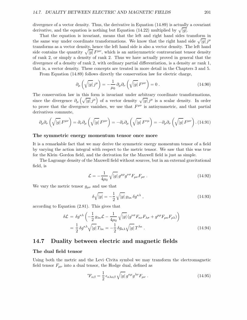
14.7. DUALITY BETWEEN ELECTRIC AND MAGNETIC FIELDS 201
divergence of a vector density. Thus, the derivative in Equation (14.89) is actually a covariantderivative, and the equation is nothing but Equation (14.22) multiplied by
√|g|.
That the equation is invariant, means that the left and right hand sides transform inthe same way under coordinate transformations. We know that the right hand side
√|g| jµ
transforms as a vector density, hence the left hand side is also a vector density. The left handside contains the quantity
√|g|Fµν , which is an antisymmetric contravariant tensor density
of rank 2, or simply a density of rank 2. Thus we have actually proved in general that thedivergence of a density of rank 2, with ordinary partial differentiation, is a density av rank 1,that is, a vector density. These concepts are treated in more detail in the Chapters 3 and 5.
From Equation (14.89) follows directly the conservation law for electric charge,
∂µ
(√|g| jµ
)= − 1
µ0∂µ∂ν
(√|g|Fµν
)= 0 . (14.90)
The conservation law in this form is invariant under arbitrary coordinate transformations,
since the divergence ∂µ
(√|g| jµ
)of a vector density
√|g| jµ is a scalar density. In order
to prove that the divergence vanishes, we use that Fµν is antisymmetric, and that partialderivatives commute,
∂µ∂ν
(√|g|Fµν
)= ∂ν∂µ
(√|g|Fµν
)= −∂ν∂µ
(√|g|F νµ
)= −∂µ∂ν
(√|g|Fµν
). (14.91)
The symmetric energy momentum tensor once more
It is a remarkable fact that we may derive the symmetric energy momentum tensor of a fieldby varying the action integral with respect to the metric tensor. We saw that this was truefor the Klein–Gordon field, and the derivation for the Maxwell field is just as simple.
The Lagrange density of the Maxwell field without sources, but in an external gravitationalfield, is
L = − 1
4µ0
√|g| gµρgνσFµνFρσ . (14.92)
We vary the metric tensor gµν and use that
δ√|g| = −1
2
√|g| gλκ δg
κλ , (14.93)
according to Equation (2.81). This gives that
δL = δgκλ(−1
2gλκL − 1
4µ0
√|g| (gνσFκνFλσ + gµρFµκFρλ)
)
=1
2δgκλ
√|g|Tλκ = −1
2δgκλ
√|g|T λκ . (14.94)
14.7 Duality between electric and magnetic fields
The dual field tensor
Using both the metric and the Levi–Civita symbol we may transform the electromagneticfield tensor Fµν into a dual tensor, the Hodge dual, defined as
∗Fαβ =1
2ǫκλαβ
√|g| gκµgλνFµν . (14.95)
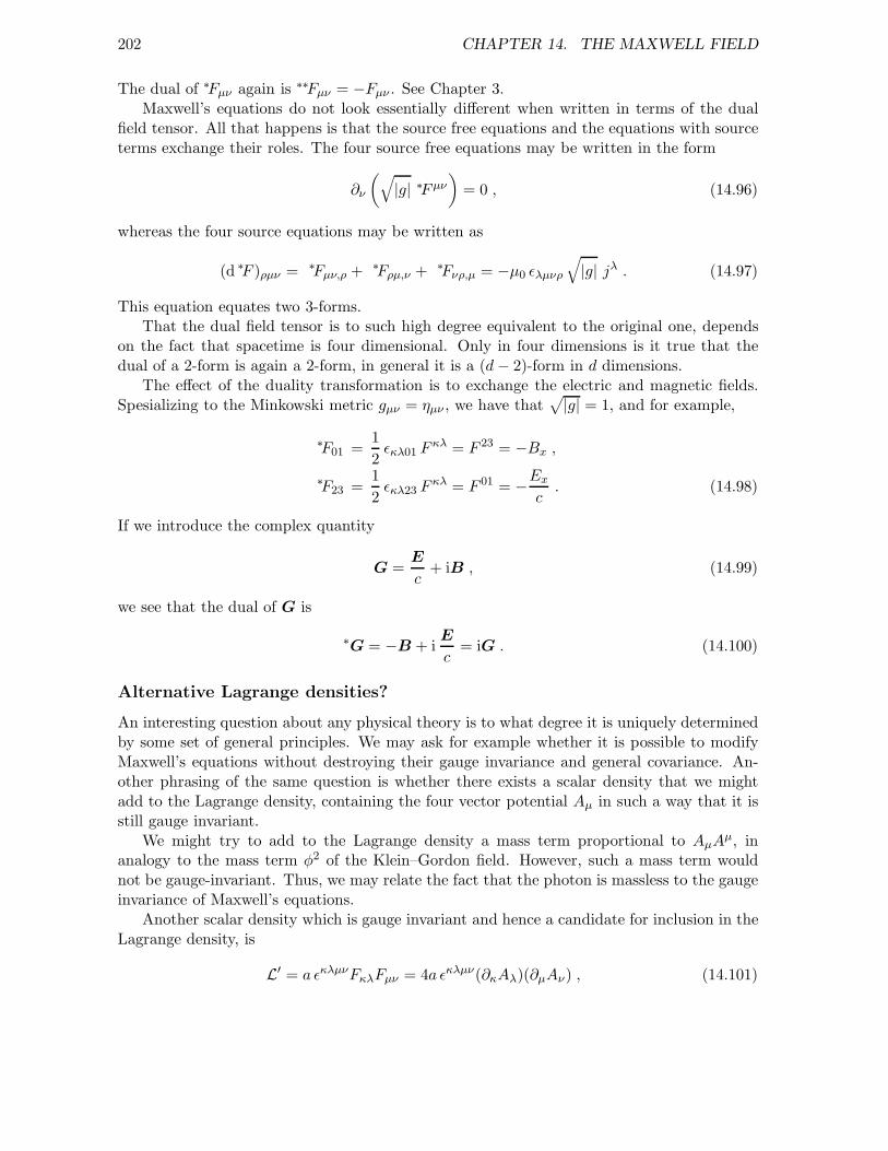
202 CHAPTER 14. THE MAXWELL FIELD
The dual of ∗Fµν again is ∗∗Fµν = −Fµν . See Chapter 3.Maxwell’s equations do not look essentially different when written in terms of the dual
field tensor. All that happens is that the source free equations and the equations with sourceterms exchange their roles. The four source free equations may be written in the form
∂ν
(√|g| ∗Fµν
)= 0 , (14.96)
whereas the four source equations may be written as
(d ∗F )ρµν = ∗Fµν,ρ + ∗Fρµ,ν + ∗Fνρ,µ = −µ0 ǫλµνρ
√|g| jλ . (14.97)
This equation equates two 3-forms.That the dual field tensor is to such high degree equivalent to the original one, depends
on the fact that spacetime is four dimensional. Only in four dimensions is it true that thedual of a 2-form is again a 2-form, in general it is a (d− 2)-form in d dimensions.
The effect of the duality transformation is to exchange the electric and magnetic fields.Spesializing to the Minkowski metric gµν = ηµν , we have that
√|g| = 1, and for example,
∗F01 =1
2ǫκλ01 F
κλ = F 23 = −Bx ,
∗F23 =1
2ǫκλ23 F
κλ = F 01 = −Ex
c. (14.98)
If we introduce the complex quantity
G =E
c+ iB , (14.99)
we see that the dual of G is
∗G = −B + iE
c= iG . (14.100)
Alternative Lagrange densities?
An interesting question about any physical theory is to what degree it is uniquely determinedby some set of general principles. We may ask for example whether it is possible to modifyMaxwell’s equations without destroying their gauge invariance and general covariance. An-other phrasing of the same question is whether there exists a scalar density that we mightadd to the Lagrange density, containing the four vector potential Aµ in such a way that it isstill gauge invariant.
We might try to add to the Lagrange density a mass term proportional to AµAµ, in
analogy to the mass term φ2 of the Klein–Gordon field. However, such a mass term wouldnot be gauge-invariant. Thus, we may relate the fact that the photon is massless to the gaugeinvariance of Maxwell’s equations.
Another scalar density which is gauge invariant and hence a candidate for inclusion in theLagrange density, is
L′ = a ǫκλµνFκλFµν = 4a ǫκλµν(∂κAλ)(∂µAν) , (14.101)
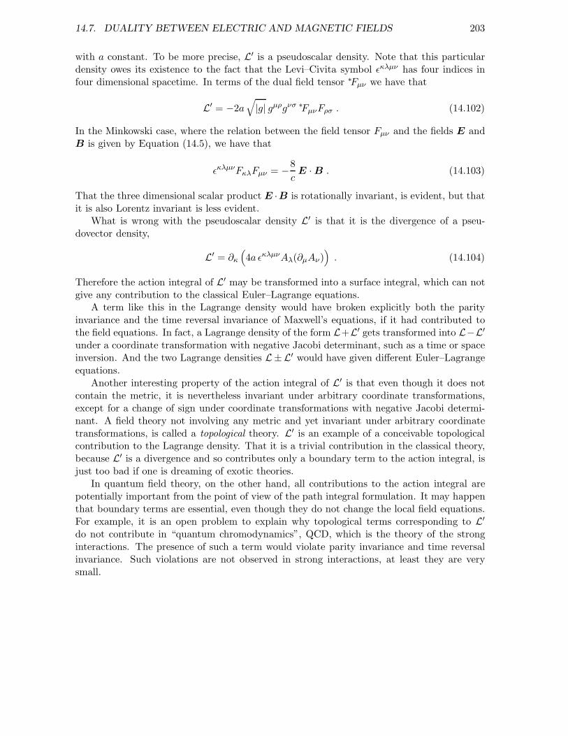
14.7. DUALITY BETWEEN ELECTRIC AND MAGNETIC FIELDS 203
with a constant. To be more precise, L′ is a pseudoscalar density. Note that this particulardensity owes its existence to the fact that the Levi–Civita symbol ǫκλµν has four indices infour dimensional spacetime. In terms of the dual field tensor ∗Fµν we have that
L′ = −2a√|g| gµρgνσ ∗FµνFρσ . (14.102)
In the Minkowski case, where the relation between the field tensor Fµν and the fields E andB is given by Equation (14.5), we have that
ǫκλµνFκλFµν = −8
cE · B . (14.103)
That the three dimensional scalar product E ·B is rotationally invariant, is evident, but thatit is also Lorentz invariant is less evident.
What is wrong with the pseudoscalar density L′ is that it is the divergence of a pseu-dovector density,
L′ = ∂κ
(4a ǫκλµνAλ(∂µAν)
). (14.104)
Therefore the action integral of L′ may be transformed into a surface integral, which can notgive any contribution to the classical Euler–Lagrange equations.
A term like this in the Lagrange density would have broken explicitly both the parityinvariance and the time reversal invariance of Maxwell’s equations, if it had contributed tothe field equations. In fact, a Lagrange density of the form L+L′ gets transformed into L−L′
under a coordinate transformation with negative Jacobi determinant, such as a time or spaceinversion. And the two Lagrange densities L±L′ would have given different Euler–Lagrangeequations.
Another interesting property of the action integral of L′ is that even though it does notcontain the metric, it is nevertheless invariant under arbitrary coordinate transformations,except for a change of sign under coordinate transformations with negative Jacobi determi-nant. A field theory not involving any metric and yet invariant under arbitrary coordinatetransformations, is called a topological theory. L′ is an example of a conceivable topologicalcontribution to the Lagrange density. That it is a trivial contribution in the classical theory,because L′ is a divergence and so contributes only a boundary term to the action integral, isjust too bad if one is dreaming of exotic theories.
In quantum field theory, on the other hand, all contributions to the action integral arepotentially important from the point of view of the path integral formulation. It may happenthat boundary terms are essential, even though they do not change the local field equations.For example, it is an open problem to explain why topological terms corresponding to L′
do not contribute in “quantum chromodynamics”, QCD, which is the theory of the stronginteractions. The presence of such a term would violate parity invariance and time reversalinvariance. Such violations are not observed in strong interactions, at least they are verysmall.
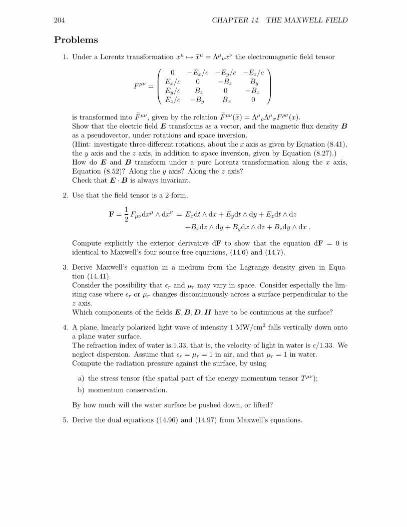
204 CHAPTER 14. THE MAXWELL FIELD
Problems
1. Under a Lorentz transformation xµ 7→ xµ = Λµνx
ν the electromagnetic field tensor
Fµν =
0 −Ex/c −Ey/c −Ez/cEx/c 0 −Bz By
Ey/c Bz 0 −Bx
Ez/c −By Bx 0
is transformed into Fµν , given by the relation Fµν(x) = ΛµρΛ
µσF
ρσ(x).Show that the electric field E transforms as a vector, and the magnetic flux density B
as a pseudovector, under rotations and space inversion.(Hint: investigate three different rotations, about the x axis as given by Equation (8.41),the y axis and the z axis, in addition to space inversion, given by Equation (8.27).)How do E and B transform under a pure Lorentz transformation along the x axis,Equation (8.52)? Along the y axis? Along the z axis?Check that E · B is always invariant.
2. Use that the field tensor is a 2-form,
F =1
2Fµνdxµ ∧ dxν = Exdt ∧ dx+ Eydt ∧ dy + Ezdt ∧ dz
+Bxdz ∧ dy +Bydx ∧ dz +Bzdy ∧ dx .
Compute explicitly the exterior derivative dF to show that the equation dF = 0 isidentical to Maxwell’s four source free equations, (14.6) and (14.7).
3. Derive Maxwell’s equation in a medium from the Lagrange density given in Equa-tion (14.41).Consider the possibility that ǫr and µr may vary in space. Consider especially the lim-iting case where ǫr or µr changes discontinuously across a surface perpendicular to thez axis.Which components of the fields E,B,D,H have to be continuous at the surface?
4. A plane, linearly polarized light wave of intensity 1 MW/cm2 falls vertically down ontoa plane water surface.The refraction index of water is 1.33, that is, the velocity of light in water is c/1.33. Weneglect dispersion. Assume that ǫr = µr = 1 in air, and that µr = 1 in water.Compute the radiation pressure against the surface, by using
a) the stress tensor (the spatial part of the energy momentum tensor T µν);
b) momentum conservation.
By how much will the water surface be pushed down, or lifted?
5. Derive the dual equations (14.96) and (14.97) from Maxwell’s equations.
Chapter 15
Gravitation and geometry
In Newton’s theory of gravitation the potential energy of a collection of N point masses is
V = −GN∑
i=2
i−1∑
j=1
mimj
|ri − rj |= −G
N∑
i=2
∑
j<i
mimj
|ri − rj|= −G
2
N∑
i=1
∑
j 6=i
mimj
|ri − rj|. (15.1)
Here G = 6.6726 × 10⁻¹¹ m3 kg−1 s−2 is Newton’s gravitational constant. Particle i has amass mi and position ri, and an acceleration given by Newton’s second law,
mid2ri
dt2= −∂V
∂ri= −G
∑
j 6=i
mimj
|ri − rj |3(ri − rj) . (15.2)
One way to interpret this equation is that particle i moves in a gravitational field fromthe other particles, given by a scalar potential
φi(r) = −G∑
j 6=i
mj
|r − rj |, (15.3)
and has a potential energy in this gravitational field which is
Vi(ri) = mi φi(ri) . (15.4)
The scalar potential φi satisfies the second order partial differential equation
∇2φi = 4πGρi , (15.5)
where ρi is the mass density, excluding particle i,
ρi(r) =∑
j 6=i
mj δ(r − rj) . (15.6)
This field equation for the gravitational potential φi contains no time derivative. Hence, φi
has no dynamics of its own, it is purely an auxiliary quantitity that we may use when we findit useful, and throw away when we no longer need it.
The electric and magnetic forces between electric charges are mediated with a finite speedthrough an electromagnetic field described by Maxwell’s equations. Newton’s gravitationaltheory is no field theory in the same sense as electromagnetism, since it describes a forcemediated with an infinite speed. A famous quotation indicates that Newton regarded this asan essential weakness of the theory, two hundred years before Faraday and Maxwell introducedthe field concept in electromagnetism:
205
206 CHAPTER 15. GRAVITATION AND GEOMETRY
“That one body may act upon another at a distance through a vacuum, withoutthe mediation of any thing else, by and through which their action and force maybe conveyed from one to another, is to me so great an absurdity, that I believe noman, who has in philosophical matters a competent faculty of thinking, can everfall into it.”
The need for a genuine field theory of gravitation became even more obvious when Einsteinformulated his special theory of relativity, which forbids velocities greater than the speed oflight. Einstein and other physicists therefore set out to find a relativistic theory of gravitation.
Such a theory can not have exactly the same form as Maxwell’s theory, even though New-ton’s gravitational potential between point masses has nearly the same form as the Coulombpotential between point charges. One important difference between the two theories is that allmasses are positive, whereas there exist both positive and negative electric charges. Anothermain difference is the sign of the potential energy: the gravitational energy is always negative,that is, the force is always attractive, whereas the Coulomb energy is positive for charges ofthe same sign, that is, the force is then repulsive. A third difference is that there is nothing inNewton’s gravitational theory corresponding to the three dimensional electromagnetic vectorpotential, and hence the magnetic force, which is proportional to the velocity of the chargedparticle, has no obvious counterpart in the gravitational theory.
15.1 The principle of equivalence
Since the inertial mass mi, on the left hand side of Newton’s equation of motion, Equa-tion (15.2), equals the gravitational mass mi, on the right hand side, it cancels from theequation. The motion of a particle in a gravitational field is independent of the mass of theparticle, according to Newton’s theory.
In general, a mass distribution with mass density ρ = ρ(r, t) gives rise to a Newtoniangravitational potential φ satisfying the equation
∇2φ = 4πGρ . (15.7)
In this gravitational field a pointlike “test particle” with a mass m so small that it does notinfluence the mass density ρ, will have a potential energy V = mφ, and will be subject to agravitational force F = −∇V = −m∇φ. Since the force is proportional to the mass m, it isnatural to define the gravitational field as the force divided by the mass,
g =F
m= −∇φ . (15.8)
The equation of motion of the test particle is independent of its mass,
d2r
dt2= g . (15.9)
Thus, the gravitational field at the position r at the time t is the same as the accelerationof gravity there: it is the acceleration that any test particle will have when placed there.Newton’s field equation of gravitation relates the divergence of the gravitational field to themass density,
∇ · g = −4πGρ . (15.10)
15.1. THE PRINCIPLE OF EQUIVALENCE 207
Recall that Maxwell’s equations relate the electric field to the charge density in the same way.The equivalence between “heavy” mass, which is the mass you feel when holding a hammer
in your hand, and “inertial” mass, which you feel when setting the hammer in motion to hita nail, was the point of departure for Einstein’s gravitational theory, the general theory ofrelativity. Inertial and heavy mass are just two aspects of the same reality, according toEinstein. He made this principle of equivalence, as he called it, an axiom of the new theory:
There is no observable difference between gravitational forces and the inertial forcesthat are observed in an accelerated coordinate system.
Einstein took as an example an observer in an elevator without a window. There is no possibleexperiment that this enclosed observer could do inside the elevator in order to learn whetherthe elevator is accelerated, or whether it is at rest in a gravitational field. In other words, agravitational field may always be transformed away locally, that is, inside the elevator at agiven time, by means of a suitable transformation of space and time.
The principle of equivalence as stated here is actually not quite true, because the gravita-tional field from stars and planets will always be inhomogeneous. When we try to transformaway an inhomogeneous gravitational field by a coordinate transformation, there will alwaysremain a residual field which can not be transformed away. The residual gravitational forceis called a tidal force, because it gives rise to the ocean tides when the Earth is falling freelyin the gravitational field from the Sun and the Moon. We will return to the subject of tidalforces at the end of this chapter.
The basis of Einstein’s principle of equivalence was not only Newton’s theory, which is ofcourse well supported by experiments, but also a very precise experiment performed by theHungarian physicist Baron Lorand von Eotvos. The idea behind the experiment was that thedirection of the force of gravity on an object in the laboratory depends on the ratio betweenthe inertial and heavy mass of the object. In fact, the observed force of gravity is the sum oftwo components having not only different physical origins but also different directions. Theobject is attracted towards the centre of the Earth, and the attractive force is proportionalto the heavy mass. But there appears also a centrifugal force due to the acceleration of thelaboratory as it follows the rotation of the Earth, this force is directed away from the rotationaxis, and is proportional to the inertial mass. Eotvos compared different materials, and foundthat they all had the same ratio between inertial and heavy mass, to a precision of 5 × 10⁻⁹
(published in 1922). The experimental precision has later been improved to 10−12.Since the equation of motion of a particle in a gravitational field is independent of its mass,
it is possible to imagine that the particle follows a geodesic, that is, a curve in spacetime ofextremal length. The relevant “length”, in the special as well as in the general theory ofrelativity, is s = cτ , where τ is the proper time of the particle. We saw in Chapter 8 thatthe “law of the cosmic laziness” holds in the special theory of relativity, that a free particlefollows an orbit such that the proper time is maximal. It is natural to assume that the samelaw holds in a gravitational field. Then the Lagrange function will be
L = −mc√
gµν(x)dxµ
dt
dxν
dt. (15.11)
The only new aspect as compared to the special theory of relativity, Equation (10.65), is that
208 CHAPTER 15. GRAVITATION AND GEOMETRY
the metric tensor is now taken to depend on time and place, gµν = gµν(x), and in general itwill be impossible to find a coordinate system in which it is constant.
The general theory of relativity is a gravitational theory in which the metric tensorgµν = gµν(x) describes the gravitational field.
15.2 Non-relativistic limit
In order to see that Equation (15.11) makes sense, we should check that it is possible tochoose the metric in such a way that we get the correct non-relativistic limit
L→ constant +1
2mv2 −mφ , (15.12)
when the velocity v = dr/dt is small compared to the speed of light c, and when the gravita-tional potential φ is also small compared to c2. The last condition is well satisfied anywherein our solar system. The gravitational potential in the solar system has its maximum (inabsolute value) at the centre of the Sun, but is nearly as large at the surface of the Sun,where it is
φS = −G M⊙
R⊙= −1.9 × 10¹¹ m2/s2 = −2.1 × 10⁻⁶ c2 . (15.13)
Here M⊙ = 2.0 × 1030 kg is the solar mass, and R⊙ = 7.0 × 10⁸ m is the solar radius.One possible solution is to take x0 = ct, x1 = x, x2 = y, x3 = z, and
g00 = 1 +2φ
c2, g11 = g22 = g33 = −1 , all other gµν = 0 . (15.14)
From Equation (15.11) we then get the wanted result that
L = −mc2√
1 +2φ
c2− v2
c2≈ −mc2 +
1
2mv2 −mφ . (15.15)
It is worth noting that Newton’s theory holds only for velocities that are small relativeto the speed of light, and therefore the non-relativistic limit gives limited information aboutthe metric gµν . Separating the time coordinate x0 = ct from the spatial coordinates xj, withj = 1, 2, 3, in Equation (15.11), we get that
L = −mc√
g00c2 + 2g0jcdxj
dt+ gjk
dxj
dt
dxk
dt. (15.16)
We get the correct non-relativistic limit by substituting g0j = gj0 = 0 and gjk = δjk, butin this limit the velocity |v| is by definition small relative to the speed of light, hence thesecomponents of the metric are less precisely determined than g00. In order to determinepossible corrections to gjk of order φ/c2, we would have to know the equation of motion for arelativistic particle in a gravitational potential φ, when φ/c2 is small. But this is not known,at least not from Newton’s theory. These corrections to gjk can be found, however, fromEinstein’s field equations, which will be the subject of the next chapter.
15.3. GRAVITATIONAL REDSHIFT 209
15.3 Gravitational redshift
According to the metric of Equation (15.14), the proper time of a particle at rest is
dτ = dt
√
1 +2φ
c2≈ dt
(1 +
φ
c2
). (15.17)
Since the gravitational potential is negative, this means that a clock in a gravitational fieldwill be retarded compared to a clock outside the field. The ratio between two proper timesdτ1 in a gravitational potential φ1, and dτ2 in a potential φ2, is
dτ1dτ2
≈1 + φ1
c2
1 +φ2
c2
≈ 1 +φ1 − φ2
c2. (15.18)
One way to measure this effect is to compare the frequencies ν1 and ν2 of two identicallight sources at the two points. We assume that the sources are monochromatic, that theirlight is of one single frequency. The frequency is the number of oscillations, n, per timeinterval ∆t, that is,
ν1 =n1
∆t, ν2 =
n2
∆t. (15.19)
If the coordinate time interval ∆t is the same for the two sources, then
ν1
ν2=n1
n2=
∆τ1∆τ2
≈ 1 +φ1 − φ2
c2. (15.20)
This gravitational redshift, as it is called, was first observed in the spectra of so called whitedwarf stars. But it is also observed directly in terrestrial laboratories. Since the accelerationof gravity on the surface of the Earth is
g = 9.8m/s2 , (15.21)
a height difference of h = 1 m makes a difference in gravitational potential of
∆φ = gh = 9.8m2/s2 ≈ 10−16 c2 . (15.22)
Pound and Rebka measured this effect in 1960 (Physical Review Letters 4, 337 (1960)), inan experiment where the height difference was 20 m. Thus, the measured effect was of order2 × 10−15.
15.4 The equation of motion for a point mass
The action along an orbit from one point A to another point B is, according to Equa-tion (15.11),
S =
∫ B
Adt L = −mc
∫ B
Adt
√
gµν(x)dxµ
dt
dxν
dt. (15.23)
210 CHAPTER 15. GRAVITATION AND GEOMETRY
Here t denotes time, but the action is unchanged if we replace t by an arbitrary parameteru = u(t), such that the spacetime coordinates along the orbit followed by the particle aregiven as functions of u,
xµ = xµ(u) . (15.24)
In fact, a change of integration variable gives that
S = −mc∫ B
Adt
√
gµν(x)dxµ
dt
dxν
dt= −mc
∫ B
Adu
√
gµν(x)dxµ
du
dxν
du. (15.25)
The reparametrization invariance of the action integral S becomes obvious when we write
S = −m∫ B
Ads = −mc
∫ B
Adτ . (15.26)
Let us define the velocity as
w =ds
du=
√
gµν(x)dxµ
du
dxν
du, (15.27)
so that the action integral is S = −mc ∫BA duw. Hamilton’s principle applied to this action
integral gives the Euler–Lagrange equations
0 =∂w
∂xρ− d
du
∂w
∂(dxρ
du
)
=
1
2wgµν,ρ
dxµ
du
dxν
du− d
du
(1
2w
(gρν
dxν
du+ gµρ
dxµ
du
)). (15.28)
The reparametrization invariance of S means that the Euler–Lagrange equations do not deter-mine how the parameter u varies along the orbit. We take advantage of this arbitrariness tochoose u = s, this implies that w = 1, and hence the Euler–Lagrange equations get simplifiedas follows,
d
ds
(gρν
dxν
ds
)− 1
2gµν,ρ
dxµ
ds
dxν
ds= 0 . (15.29)
This may indeed be a convenient form of the equation of motion, but it is customary torewrite further by expanding the derivative,
0 = gρνd2xν
ds2+ gρν,σ
dxσ
ds
dxν
ds− 1
2gµν,ρ
dxµ
ds
dxν
ds
= gρνd2xν
ds2+
1
2(gρµ,ν + gρν,µ − gµν,ρ)
dxµ
ds
dxν
ds. (15.30)
Finally, multiplication by gλρ gives the geodesic equation,
d2xλ
ds2+ Γλ
µν
dxµ
ds
dxν
ds= 0 . (15.31)
15.5. TIDAL FORCES DUE TO GEODESIC DEVIATION 211
We recognize Γλµν as the metric and symmetric connection, also known as the Christoffel
connection. The Christoffel connection coefficients are symmetric in their lower indices, Γλµν =
Γλνµ, and are given by the metric tensor and its first order derivatives as
Γλµν =
1
2gλρ(gρµ,ν + gρν,µ − gµν,ρ) . (15.32)
We have seen in Chapter 5 that the connection Γ is not a tensor, but transforms in a differentway under coordinate transformations.
The symmetry Γλµν = Γλ
νµ is the mathematical way of expressing Einstein’s principleof equivalence, because it means that the connection may be “transformed away” at onearbitrary point by a suitable choice of coordinates. In other words, around any given pointin spacetime it is possible to introduce a local coordinate system such that all connectioncoefficients vanish at this single point.
From Equation (15.32) follows that the covariant derivative of the metric tensor vanishes,
gµν;ρ = gµν,ρ − gσνΓσµρ − gµσΓσ
νρ = 0 . (15.33)
This equation together with the geodesic equation implies that
d
ds
(gµν
dxµ
ds
dxν
ds
)= gµν,ρ
dxρ
ds
dxµ
ds
dxν
ds−(gµνΓµ
ρσ
dxν
ds+ gµν
dxµ
dsΓν
ρσ
)dxρ
ds
dxσ
ds
=(gµν,ρ − gσνΓσ
µρ − gµσΓσνρ
) dxρ
ds
dxµ
ds
dxν
ds= 0 . (15.34)
This result is important, because it demonstrates that the geodesic equation is compatiblewith the assumption that w = 1, which helped us to simplify the equation.
It is worth noting that the geodesic equation may be derived from a different Lagrangefunction, Equation (10.105),
L′ = −1
2mc2gµν(x)
dxµ
ds
dxν
ds. (15.35)
This Lagrange function fixes the parametrization of the orbit, since the action integral is notreparametrization invariant. It has the same non-relativistic limit, up to an additive constant.
15.5 Tidal forces due to geodesic deviation
Physical bodies are not point masses, and it is natural to ask what will happen to an extendedbody moving in a gravitational field. The answer, as we know from Newton’s theory, is thatit will feel the effect of an inhomogeneous field as tidal forces squeezing in some directionsand tearing in other directions. According to the geometric point of view we want to takehere, the tidal forces result from the relative accelerations of neighbouring geodesics, sinceeach part of the body tries to follow its own geodesic. We want now to calculate the relativeacceleration of two point particles.
212 CHAPTER 15. GRAVITATION AND GEOMETRY
Tidal forces according to Newton
The relative acceleration of two point particles moving in a gravitational field g = g(r, t), onealong the orbit r1 = r1(t) and the other one along the nearby orbit r2 = r2(t) = r1(t)+∆r(t),is
∆a =d2
dt2∆r = ∆g = g(r2(t), t) − g(r1(t), t) . (15.36)
If we regard the first particle as an observer observing the second particle, then the observedposition is ∆r, and the observed acceleration ∆a will be interpreted as being due to theresidual gravitational field ∆g. The three spatial components of ∆g are, to first order in ∆r,
∆gi(∆x1,∆x2,∆x3) = gi,j ∆xj , (15.37)
where the partial derivatives gi,j are computed at the position of the first particle. The linearity
in ∆r implies that the tidal forces at opposite points ∆r and −∆r balance.Note that the field equation in vacuum,
∇ · g = g1,1 + g2
,2 + g3,3 = gi
,i = 0 , (15.38)
means that the tidal forces will tend to preserve volumes. If they pull in one direction, theypush in another direction, and vice versa. The field equation does not say anything aboutwhether the tidal forces exert a torque on an extended body.
Tidal forces from geodesic motion
Now we consider one point particle moving along a geodesic xµ = xµ(s) which is a solutionof Equation (15.31), and a second point particle moving along a nearby geodesic
yµ = yµ(s) = xµ(s) + ∆xµ(s) . (15.39)
We choose to parametrize this second geodesic by the same parameter s which is the geodesicparameter of the first geodesic, but we should remember that the geodesic parameter of thesecond geodesic, let us call it s, is not necessarily equal to s. Define
w =ds
ds=
√
gµν(y)dyµ
ds
dyν
ds. (15.40)
Then the second geodesic equation,
d2yλ
ds2+ Γλ
µν(y)dyµ
ds
dyν
ds= 0 , (15.41)
may be rewritten as
wd
ds
(1
w
dyλ
ds
)+ Γλ
µν(y)dyµ
ds
dyν
ds= 0 . (15.42)
Using Equation (15.31), and assuming that both the deviation ∆xµ and its derivative withrespect to s are small, we get to first order in ∆xµ that
d2(∆xλ)
ds2− d(lnw)
ds
dxλ
ds+ Γλ
µν,ρ(x)∆xρ dxµ
ds
dxν
ds+ 2Γλ
µν(x)dxµ
ds
d(∆xν)
ds= 0 . (15.43)
15.5. TIDAL FORCES DUE TO GEODESIC DEVIATION 213
If we again regard the first particle as an observer of the motion of the second particle, thelocal time axis at one point on the observer’s geodesic trajectory is the unit tangent vector
eµ(0) =dxµ
ds. (15.44)
We now expand
∆xµ =3∑
i=1
ξ(i)eµ(i) , (15.45)
where eµ(i) for i = 1, 2, 3 are unit vectors orthogonal to the time axis eµ(0) and to each other.
That is, for α, β = 0, 1, 2, 3, and for any point xµ = xµ(s) along the geodesic, we have that
gµν(x) eµ(α) eν(β) = ηαβ =
1 0 0 00 −1 0 00 0 −1 00 0 0 −1
. (15.46)
Equation (15.31), the geodesic equation, means simply that the tangent vector eµ(0) is parallel
transported along the curve. We now require that also the three normal vectors eµ(i) fori = 1, 2, 3 should be parallel transported, so that for α = 0, 1, 2, 3 we have
d(eµ(α))
ds+ Γµ
σρ eσ(α)
dxρ
ds=
d(eµ(α))
ds+ Γµ
σρ eσ(α) e
ρ(0) = 0 . (15.47)
The physical meaning is that when the four unit vectors are parallel transported alongthe geodesic, they come as close as possible to defining a local inertial frame. We may call itthe “local Lorentz frame”, or with a longer expression, the “instantaneous rest frame of thefirst particle”. Thus, the three spatial coordinates ξ(1), ξ(2), ξ(3), which we assume to be small,are what we may call “local Euclidean coordinates”. The velocity and acceleration relativeto the local Euclidean reference frame is respectively the first and second derivative of thesecoordinates with respect to the proper time τ = s/c,
dξ(i)
dτ= c
dξ(i)
ds,
d2ξ(i)
dτ2= c2
d2ξ(i)
ds2. (15.48)
In order to simplify a little bit, we ask for the acceleration d2ξ(i)/dτ2 at a moment whenthe velocity dξ(i)/dτ is zero. With this simplification we have that
d(∆xµ)
ds=
dξ(i)
dseµ(i) + ξ(i)
d(eµ(i))
ds= −ξ(i) Γµ
σρ eρ(0) e
σ(i) , (15.49)
and further that
d2(∆xµ)
ds2=
d2ξ(i)
ds2eµ(i) + 2
dξ(i)
ds
d(eµ(i))
ds+ ξ(i)
d2(eµ(i))
ds2
=d2ξ(i)
ds2eµ(i) + ξ(i)
d2(eµ(i))
ds2. (15.50)
214 CHAPTER 15. GRAVITATION AND GEOMETRY
Here we have that
d2(eµ(i))
ds2= − d
ds
(Γµ
σρ eσ(i) e
ρ(0)
)
= −(Γµσρ,κ e
κ(0)) e
σ(i) e
ρ(0) + Γµ
σρ (Γσκλ e
κ(i) e
λ(0)) e
ρ(0) + Γµ
σρ eσ(i) (Γρ
κλ eκ(0) e
λ(0)) (15.51)
=(−Γµ
σρ,κ + Γµτρ Γτ
σκ + Γµστ Γτ
κρ
)eκ(0) e
σ(i) e
ρ(0) .
Altogether, Equation (15.43), which describes geodesic deviation, takes the following format a moment when dξ(i)/ds = 0,
d2ξ(i)
ds2eλ(i) −
d(lnw)
dseλ(0) + ξ(i)
((−Γλ
σρ,κ + Γµτρ Γτ
σκ + Γµστ Γτ
κρ
)eκ(0) e
σ(i) e
ρ(0)
+ Γλµν,ρ e
ρ(i) e
µ(0) e
ν(0) − 2Γλ
µν(x) eµ(0) Γµ
σρ eρ(0) e
σ(i)
)= 0 . (15.52)
Introducing the Riemann curvature tensor, we write the equation as follows,
d2ξ(i)
ds2eλ(i) −
d(lnw)
dseλ(0) + ξ(i)Rλ
µρν eµ(0) e
ρ(i) e
ν(0) = 0 . (15.53)
Let us introduce the inverse of the 4× 4 matrix eµ(α), written as e(α)µ and defined by either
one of the two relations
e(β)µ eµ(α) = δβ
α , eµ(α) e(α)ν = δµ
ν . (15.54)
We may then introduce the components of the Riemann curvature tensor relative to the localLorentz frame,
R(α)(β)(γ)(δ) = Rλ
µρν e(α)λ eµ(β) e
ρ(γ) e
ν(δ) , (15.55)
and write the equation of geodesic deviation in the following simple way,
d2ξ(i)
dτ2+ c2ξ(j)R(i)
(0)(j)(0) = 0 . (15.56)
This equation gives a direct physical meaning to the Riemann curvature tensor. In fact,the tidal forces experienced by an extended body moving in a gravitational field are describedlocally by a residual gravitational field of Newtonian type,
g(i)(ξ(1), ξ(2), ξ(3)) = −c2ξ(j)R(i)(0)(j)(0) . (15.57)
Remember that the two indices (0) refer to the local time axis, which is the tangent to thegeodesic xµ(s) followed by our reference particle.
15.5. TIDAL FORCES DUE TO GEODESIC DEVIATION 215
Problems
1. Find explicitly the equations for geodesic lines in the following examples.
a) The plane, with coordinates (x, y) and metric ds2 = dx2 + dy2.
b) Same as a), but in polar coordinates (r, ϕ).
c) The surface of a sphere, in polar coordinates (θ, ϕ).
Find the general solution in each example. (See the problems 3, 4 and 5 of Chapter 2.)
2. The acceleration of gravity on the surface of the Earth is g = 9.81 m/s2, in this problemwe take g = 10 m/s2 for simplicity. A tiny ball thrown up into the air with a velocity ofexactly 5 m/s will then come back down exactly one second later, ignoring the frictionagainst the air.What is the proper time of the ball for the round trip up and down?Two effects influence the proper time: the special relativistic time dilation, and thegravitational field. What is the sign of each of the two effects, and which effect is thelargest? Are your answers consistent with the principle of cosmic laziness? Why mustthe two effects necessarily be of roughly the same magnitude?Make similar calculations for an artificial sattelite in a circular orbit 500 km above thesurface of the Earth, and for the Moon.
216 CHAPTER 15. GRAVITATION AND GEOMETRY
Chapter 16
Einstein’s gravitational equation
The gravitational field influences point particles and other fields, such as the Klein–Gordonfield and the Maxwell field, because the metric tensor gµν enters in the Lagrange functionsfor point particles and in the Lagrange densities for fields. In principle, the first derivativesof the metric tensor might enter through the connection coefficients Γλ
µν , but this does nothappen in those examples we have seen so far.
Einstein’s equation for the gravitational field is a second order differential equation forthe metric tensor. The second order derivatives enter through the curvature tensor, whichcontains the connection coefficients and their first derivatives. The gravitational field equationgives a direct relation between the curvature of the four dimensional spacetime and the totalenergy momentum tensor of all particles and all fields, except for the gravitational field.
16.1 Einstein’s field equation
According to Newton’s gravitational theory, the divergence of the gravitational field vanisheswhen the mass density vanishes,
∇ · g = 0 . (16.1)
This is the field equation in vacuum. Applying this equation to the local gravitational field inEquation (15.57), computed from the equation of geodesic deviation, gives the field equation
R(i)(0)(i)(0) = 0 . (16.2)
There is a sum over i = 1, 2, 3, but we may include i = 0 in the sum, because the antisymmetryproperty R(α)
(β)(γ)(δ) = −R(α)(β)(δ)(γ) implies that R(0)
(0)(0)(0) = 0. Then we obtain the Riccicurvature tensor, and the field equation is
R(α)(0)(α)(0) = R(0)(0) = Rµν e
µ(0) e
ν(0) = 0 . (16.3)
This is the gravitational field equation in one particular local Lorentz frame, with a givenlocal time axis eµ(0). But the requirement of invariance under general coordinate transforma-
tions implies that this equation must hold for an arbitrary timelike unit vector eµ(0), and theonly way that can be true, is that the Ricci tensor vanishes identically,
Rµν = 0 . (16.4)
217

218 CHAPTER 16. EINSTEIN’S GRAVITATIONAL EQUATION
This is Einstein gravitational field equation in vacuum. The Ricci tensor enters the equationbecause it is the trace of the Riemann tensor, which describes the residual gravitational fieldseen in a local inertial frame.
The field equation with a source term can be obtained by a similar reasoning, but thereis some subtlety involved. Newton’s equation, with the mass density ρ as the source,
∇ · g = −4πGρ , (16.5)
would now take the form
c2R(0)(0) = 4πGρ . (16.6)
Einstein wanted to replace the mass density ρ by the energy density ρc2, which is the com-ponent T(0)(0) of the energy momentum tensor Tµν . This gives the equation
R(0)(0) =4πG
c4T(0)(0) , (16.7)
which holds in the case of a non-relativistic mass distribution, with T(0)(0) = ρc2, with T(i)(0) =T(0)(i) = 0 and T(i)(j) = 0 for i, j = 1, 2, 3. The obvious generalization would be the equation
Rµν =4πG
c4Tµν , (16.8)
and this was indeed Einstein’s first guess. However, he soon discovered that it needs somemodification, because it is inconsistent with the conservation of energy and momentum. Wenow jump directly to the correct equation.
Given a metric and symmetric connection, the Einstein curvature tensor is defined as
Gµν = Rµν − 1
2gµνR . (16.9)
It is symmetric, and due to the contracted Bianchi identity, Equation (6.54), it has zerodivergence,
Gµν;ν = Rµν
;ν − 1
2gµνR,ν = Rµν
;ν − gµνgρσRρν;σ = Rµν;ν −Rσµ
;σ = 0 . (16.10)
For these two reasons, and because it is a tensor containing second order derivatives of themetric tensor gµν , Einstein proposed to place it on the left hand side of a field equationhaving the energy momentum tensor as a source, on the right hand side. This is Einstein’sgravitational equation,
Gµν = κTµν . (16.11)
Since the divergence of Gµν vanishes identically, the equation guarantees the conservation ofenergy and momentum, in a similar way as Maxwell’s equations guarantee the conservationof electric charge.
16.2. STATIC MASS DISTRIBUTION AND WEAK FIELD 219
Einstein’s gravitational constant κ is proportional to Newton’s gravitational constant G.The relation between them can be found by comparison with Equation (16.7), as we will doimmediately below, or equivalently by comparison with the approximate equations (15.5) and(15.14), as we will do in the next section.
The trace of the Einstein tensor is
gµνGµν = gµνRµν − 1
2gµνgµνR = R− 2R = −R . (16.12)
Hence, by taking the trace of Einstein’s equation, we find that the scalar curvature R isproportional to the trace T = gµνTµν of the energy momentum tensor,
R = −κT . (16.13)
This means that we may write the gravitational equation in another way which is equivalent,
Rµν = κ
(Tµν − 1
2gµνT
). (16.14)
A special case is the gravitational equation in vacuum, Rµν = 0.In the non-relativistic case, Equation (16.14) gives the equation
R00 = κ
(T00 −
1
2g00T
)=κ
2T00 =
κ
2ρc2 . (16.15)
Comparing with Equation (16.7), we see that
κ =8πG
c4. (16.16)
16.2 Static mass distribution and weak field
The first test for Einstein’s theory is that it must reproduce the results from Newton’s theoryin the non-relativistic limit. Thus, we have to look for an approximate solution of Einstein’sfield equation corresponding to Newton’s gravitational potential φ from masses lying at rest,and we start by assuming that
T 00 = ρc2, all other T µν = 0 , (16.17)
where ρ is the density of rest mass. Strictly speaking, the stress tensor T kl with k, l = 1, 2, 3can not vanish if the mass distribution is to be static, but we may anyway assume that it isnegligible compared to the energy density T 00. In addition, we assume that the field is weak,in the sense that φ/c2 is small. Although we make assumptions about the mass distributionthat is the source of the field, we no longer make any assumptions about the velocities of theparticles moving in the field.
220 CHAPTER 16. EINSTEIN’S GRAVITATIONAL EQUATION
That the field is weak, must mean that the metric is the special relativistic Minkowskimetric ηµν plus a small perturbation,
gµν = ηµν + hµν . (16.18)
We may imagine a Taylor series development to first order in a small parameter ǫ, such thathµν = ǫhµν , with hµν of the same order as ηµν . To zeroth order in ǫ we have gµν = ηµν . Wemay easily verify that
gµν = ηµν − hµν (16.19)
to first order in ǫ, when we define hµν = ηµρηνσhρσ . Furthermore, to first order in ǫ we havethat
Γκλµ =
1
2ηκρ (hρλ,µ + hρµ,λ − hλµ,ρ) , (16.20)
and that
Rλν = Γκλν,κ − Γκ
λκ,ν =1
2ηκρ (hρν,λκ − hλν,ρκ − hρκ,λν + hλκ,ρν) . (16.21)
The scalar curvature is, to the same order,
R = ηλνRλν = ηλνηκρ (hρν,λκ − hλν,ρκ) , (16.22)
whereas Einstein’s tensor is Gµν = Rµν − (1/2)ηµνR.Since the left hand side of the gravitational equation is of first order in the parameter ǫ,
the energy momentum tensor, on the right hand side, must also be of first order in ǫ, i.e.,T µν = ǫT µν with T µν finite. We have to first order that Tµν = ηµρηνσT
ρσ. The two equivalentforms of the gravitational equation, Equations (16.11) and (16.14), then take the followingfirst order forms. Either
ηρσ (hρµ,νσ + hρν,µσ − hµν,ρσ − hρσ,µν) − ηµνηαβηρσ (hρα,βσ − hαβ,ρσ) = 2κTµν , (16.23)
or
ηρσ (hρµ,νσ + hρν,µσ − hµν,ρσ − hρσ,µν) = κ (2Tµν − ηµνT ) . (16.24)
Both are linear second order differential equations for hµν .The first order version of the identity Gµν
;ν = 0 says that Gµν,ν = 0, where Gµν =
ηµρηνσGρσ . The conservation law for energy and momentum, T µν;ν = 0, which is a consistency
condition for the gravitational equation, also has a first order version, which is that T µν,ν = 0,
since the difference
T µν;ν − T µν
,ν = ΓµρνT
ρν + ΓνρνT
µρ (16.25)
is of second order. We may verify that the equation T µν,ν = 0 is precisely the consistency
condition for Equation (16.23), and hence also for Equation (16.24). But T µν,ν = 0 is the
special relativistic conservation law, in which the acceleration due to the gravitational field isnot taken into account. Thus, to first order in ǫ there is no back reaction from the gravitationalfield on matter. With the energy momentum tensor of Equation (16.17), the four equations
16.3. DEFLECTION OF LIGHT 221
T µν,ν = 0 reduce to the one equation T 00
,0 = 0, saying that the mass density ρ is timeindependent.
With a static mass distribution it is natural to look for a static solution of the fieldequation for the metric. Thus, let us assume that hµν,0 = 0, and use Equation (16.24), whichis the simplest version to use here. We also insert T = ηµνTµν = T00 = ρc2. Then there arealtogether ten equations to be solved, we must e.g. let the indices µ and ν take all values0 ≤ µ ≤ ν ≤ 3.
Taking first µ = ν = 0, we get the equation
∇2h00 = κρc2 . (16.26)
From the Equations (15.14) and (15.5) we know that
h00 =2φ
c2, ∇2φ = 4πGρ . (16.27)
Thus far, we get the non-relativistic limit of Einstein’s theory to agree with Newton’s theorywhen we choose Einstein’s gravitational constant to be given by Newton’s constant as κ =8πG/c4, the same relation we found before.
In order to solve the remaining nine equations it is sufficient to consider the three typicalcases µν = 11, 01 and 12, giving the equations
−2(h11,11 + h21,12 + h31,13) + ∇2h11 − h,11 = κρc2 ,
−h10,11 − h20,12 − h30,13 + ∇2h01 = 0 , (16.28)
−h11,21 − h21,22 − h31,23 − h12,11 − h22,12 − h32,13 + ∇2h12 − h,12 = 0 .
Here we have introduced
h = ηµνhµν = h00 − h11 − h22 − h33 . (16.29)
All these three equations, and in the same way all the six equations we did not write outexplicitly, are solved by the first order metric
h00 = h11 = h22 = h33 =2φ
c2, all other hµν = 0 . (16.30)
16.3 Deflection of light
Now that we know all the components of the metric gµν to order φ/c2, we are able to computehow a particle moves in a gravitational field when its velocity approaches the speed of light.In particular, we are able to compute the deflection of light.
The metric is, to first order in φ/c2,
g00 = 1 +2φ
c2, g11 = g22 = g33 = −1 +
2φ
c2, all other gµν = 0 . (16.31)
For simplicity we assume that the gravitational potential φ is static.The connection coefficients are given by Equation (15.32), and to order φ/c2 they are
Γ0µν =
1
2(g0µ,ν + g0ν,µ) ,
Γjµν = −1
2(gjµ,ν + gjν,µ − gµν,j) . (16.32)
222 CHAPTER 16. EINSTEIN’S GRAVITATIONAL EQUATION
As usual, we let greek indices run from 0 to 3 and latin indices from 1 to 3. The nonvanishingcoefficients to order φ/c2 are
Γ00j = Γ0
j0 = Γj00 =
1
2g00,j =
1
c2φ,j ,
Γjkl = − 1
c2(δjk φ,l + δjl φ,k − δkl φ,j) . (16.33)
For the time coordinate x0 the geodesic equation gives that
d2x0
ds2= −Γ0
µν
dxµ
ds
dxν
ds= − 2
c2φ,j
dx0
ds
dxj
ds= − 2
c2dx0
ds
dφ
ds. (16.34)
This equation may be integrated once exactly, and gives then that
dx0
ds= Ke−2φ/c2 = K
(1 − 2φ
c2
), (16.35)
where K is an integration constant. We may for example choose K = c, then the parameters corresponds approximately to the time t. We compute all the way through to first order inφ/c2.
For the space coordinate xj the geodesic equation gives that
d2xj
ds2= −Γj
00
(dx0
ds
)2
− Γjkl
dxk
ds
dxl
ds
= − 1
c2φ,j
(dx0
ds
)2
+2
c2φ,k
dxj
ds
dxk
ds− 1
c2φ,j δkl
dxk
ds
dxl
ds. (16.36)
When the curve xµ = xµ(s) describes a light ray, its tangent dxµ/ds is a null vector,
0 = gµνdxµ
ds
dxν
ds=
(1 +
2φ
c2
)(dx0
ds
)2
−(
1 − 2φ
c2
)δjk
dxj
ds
dxk
ds. (16.37)
With dx0/ds as above, and with K = c, this means that
δjkdxj
ds
dxk
ds= c2 . (16.38)
Thus we arrive at the following equation, to first order,
d2xj
ds2= −2φ,j +
2
c2φ,k
dxj
ds
dxk
ds. (16.39)
That the field is weak, means that the light ray is approximately a straight line. Wechoose our coordinate system and our zero point for the parameter s such that the straightline is given by the equations x = cs, y = y0 = constant and z = z0 = constant. The equationof motion for x,
d2x
ds2= −2
∂φ
∂x+
2
c2dx
ds
(∂φ
∂x
dx
ds+∂φ
∂y
dy
ds+∂φ
∂z
dz
ds
), (16.40)
16.3. DEFLECTION OF LIGHT 223
holds when we insert x = cs and dy/ds = dz/ds = 0. The deflection is given by the equationsfor y and z,
d2y
ds2= −2
∂φ
∂y+
2
c2∂φ
∂x
dy
ds
dx
ds= −2
∂φ
∂y,
d2z
ds2= −2
∂φ
∂z+
2
c2∂φ
∂x
dz
ds
dx
ds= −2
∂φ
∂z. (16.41)
It is interesting to compare the deflection computed here with the one that Newton’sequation of motion would give. According to Newton, the acceleration of a particle in agravitational field is
d2xj
dt2= −φ,j , (16.42)
independent of the mass and velocity of the particle. If the velocity equals the speed of lightc, and if we choose coordinates such that the light ray follows approximately the straight linex = ct, y = y0, z = z0, then the deflection is given, according to Newton, by the equations
d2y
dt2= −∂φ
∂y,
d2z
dt2= −∂φ
∂z. (16.43)
We see that Einstein’s theory predicts twice as much deflection as Newton’s theory fora particle moving with the speed of light. Remember that the most important requirementthat Einstein imposed on his new theory, was that it had to agree with Newton’s theoryin the case of a particle moving with a small velocity. The reason for the factor of twobetween the predictions of the two theories when the velocities are large, is not too difficultto see. Newton’s theory is the non-relativistic limit of Einstein’s theory, and in this limitthe gravitational potential φ is retained only in the time component g00 of the metric. Aswe have seen, the gravitational potential gives equally large first order corrections to all thefour diagonal elements of the metric, but the corrections to the spatial components gjk ofthe metric give noticeable contributions in the equation of motion only for particles havingvelocities comparable to the speed of light.
As a concrete example, let φ be the gravitational potential from a point mass M at theorigin,
φ = −G M
r, (16.44)
with r =√x2 + y2 + z2. We choose our coordinate system such that z = z0 = 0, and get the
following equation to solve,
d2y
ds2= −2
∂φ
∂y= −2G
My0
(x2 + y02)3/2
. (16.45)
The total deflection is
∆
(dy
ds
)= −2GMy0
∫ ∞
−∞
ds
(c2s2 + y02)3/2
= −4GM
cy0, (16.46)
since∫ ∞
−∞
ds
(c2s2 + y2)3/2=
s
y2√c2s2 + y2
∣∣∣∣∣
∞
−∞
=2
cy2. (16.47)
224 CHAPTER 16. EINSTEIN’S GRAVITATIONAL EQUATION
The angle of deflection, found by division with dx/ds = c, is
α = −4GM
c2y0. (16.48)
For a light ray passing just above the surface of the Sun, the angle is
|α| = 8, 5 × 10−6 = 1, 75′′ . (16.49)
We have inserted here the mass of the Sun, M = 2, 0 × 1030 kg, and the radius of the Sun,y0 = 7, 0 × 108 m. According to Newton’s theory the deflection should be half as much.Compare the angle of 1, 75′′ to the angular diameters of the discs of the Sun and the Moon,both about 30′ = 1800′′, that is, about one thousand times larger.
Arthur Eddington measured the deflection of the light from a star at the edge of the Sunduring a total solar eclipse in 1919. He concluded that Einstein’s theory is correct. However,his measurement was not an easy one, and did perhaps not convince everybody. Today,radio astronomers are able to measure angles with such impressive precision that they haveto correct for the deflection of radio waves in the gravitational field of the Sun, even whenobserving in directions at 90 degrees relative to the Sun.
16.4 Linearized gravitational theory
The linearized gravitational Equation (16.23), or the equivalent Equation (16.24), is an inter-esting field equation in itself, irrespective of its derivation as an approximation to Einstein’sequation. We have seen one way we may use it to compare the theories of Einstein andNewton. If the souce T µν is not static, but oscillates, then the same equation predicts a newphenomenon, gravitational radiation. We will not study gravitational radiation here, insteadwe will take a look at how the invariance of Einstein’s equation under general coordinatetransformations is expressed in the linearized equation.
Then we consider a coordinate transformation of the form
xµ 7→ xµ = xµ + ξµ , (16.50)
where ξµ = ξµ(x) = ǫξµ(x) is a small quantity, proportional to the small parameter ǫ. Asusual, we compute only to first order in ǫ.
The energy momentum tensor T µν is already of first order in ǫ, and it is invariant to firstorder under the small coordinate transformation, since every possible correction has to besecond order. The metric tensor is transformed as follows,
gµν(x) =∂xρ
∂xµ
∂xσ
∂xνgρσ(x) . (16.51)
The matrix ∂xρ/∂xµ is the inverse of
∂xµ
∂xρ= δµ
ρ + ξµ,ρ , (16.52)
and it is, to first order,
∂xρ
∂xµ= δρ
µ − ξρ,µ . (16.53)

16.5. THE GEODESIC EQUATION FOLLOWS FROM THE FIELD EQUATION 225
Thus we have, to first order,
gµν(x) = (δρµ − ξρ
,µ) (δσν − ξσ
,ν) gρσ(x− ξ) . (16.54)
Since gµν = ηµν + hµν with hµν proportional to ǫ, we have to first order in ǫ that
gµν(x− ξ) = gµν(x) − ξρgµν,ρ(x) = gµν(x) − ξρhµν,ρ(x) = gµν(x) . (16.55)
Thus, the field hµν transforms as follows, with ξµ = ηµρξρ,
hµν = hµν − ξσ,ν ηρµ − ξρ
,µ ησν = hµν − ξµ,ν − ξν,µ . (16.56)
We see that a small coordinate transformation acts as a kind of gauge transformation ofthe linearized gravitational field, in analogy to the gauge transformationen Aµ = Aµ − χ,µ
of the electromagnetic four vector potential. We see also directly that the left hand sides ofboth Equations (16.23) and (16.24) are invariant under this kind of gauge transformation.
16.5 The geodesic equation follows from the field equation
We postulated from the beginning that a “test particle”, i.e. a point particle having such asmall mass that it does not contribute essentially to the gravitational field, moves along ageodesic curve in spacetime. This postulate is actually superfluous, because it follows fromthe field equation Gµν = κTµν .
As we have seen, the field equation implies that the energy momentum tensor is conserved,
T µν;ν = 0 , (16.57)
since Gµν;ν = 0 identically. That the field equation had to guarantee the conservation of the
source, was an important clue to Einstein in his search for the right equation. His model inthis respect was Maxwell’s equations, which guarantee the conservation of electric charge. Animportant difference between the two cases is that the electric charge is a scalar, and henceits conservation is expressed in one single continuity equation. Energy and momentum, onthe other hand, are components of a four vector, and as a consequence, the conservation lawT µν
;ν = 0 gives four equations, which are no less than complete equations of motion for theparticles that are the sources of the field.
To see this, we consider as an example a collection of “dust”, or to put it differently, anideal gas without pressure, i.e. at zero temperature. If there are sufficiently many particles wemay describe the gas approximately as a continuum, and if they are sufficiently small, theywill have no appreciable influence on the metric. One single particle of mass m will followan orbit in spacetime which may be parametrized by the proper time τ of this particle, asxµ = xµ(τ). The energy and momentum of the particle are the four componentene of thefour vector pµ = muµ, where uµ is the four velocity, defined as
uµ =dxµ
dτ. (16.58)
The definition of the proper time τ is that
uµuµ = c2 = constant , (16.59)
226 CHAPTER 16. EINSTEIN’S GRAVITATIONAL EQUATION
and the equation of motion for the particle that we want to derive, is the geodesic equation
d2xµ
dτ2+ Γµ
ρσ
dxρ
dτ
dxσ
dτ=
duµ
dτ+ Γµ
ρσ uρuσ = 0 . (16.60)
We asume that all the particles together may be described by a velocity field uµ = uµ(x),and in addition a function ρ = ρ(x) which is the mass density in the rest system of theparticles passing by the spacetime point x. We want to show that Equation (16.60) followsfrom Equation (16.57) when the energy momentum tensor is
T µν = ρuµuν . (16.61)
Inserting in Equation (16.57) we get that
(ρuν);ν uµ + ρuνuµ
;ν = 0 . (16.62)
Multiplying this equation by uµ gives that
(ρuν);ν = 0 , (16.63)
since uµuµ = c2, and hence
uµuµ;ν =
1
2(uµu
µ);ν = 0 . (16.64)
It follows that
uνuµ;ν = 0 . (16.65)
This equation is precisely the geodesic equation, since
uνuµ;ν =
dxν
dτ
(uµ
,ν + Γµρνu
ρ)
=duµ
dτ+ Γµ
ρνuρuν . (16.66)
16.6 The cosmological constant
Einstein arrived at his field equation in 1915, but modified it in 1917, because he wanted theequation to have a static solution which could describe the Universe as a whole. His modifi-cation was to introduce an extra term, containing a new constant Λ, called the cosmologicalconstant, such that the equation takes the form
Gµν − Λgµν = κT µν . (16.67)
He regretted later the introduction of the new term, and called it “the blunder of my life”. Infact, the cosmological constant did not solve the problem it was intended to solve. Formally,it results in the existence of solutions describing a static Universe, but these solutions can notbe realized physically, because they are unstable.
If Einstein had not changed the equation, he would have predicted the cosmic redshift oflight from distant galaxies, detected by Edwin Hubble during the next decade, and showing
16.6. THE COSMOLOGICAL CONSTANT 227
that the Universe is expanding. However, the question of whether or not the cosmological con-stant is exactly zero, is in the end an experimental question. Since the modified gravitationalequation may be written as
Gµν = κ
(T µν +
Λ
κgµν
), (16.68)
we may interpret Λ/κ as an extra energy density, which is then thought of as a vacuum energydensity. A crude upper limit for this energy density is the average mass density in a typicalcluster of galaxies, which is around ρ0 = 10−26 kg/m3. The fact that Newton’s equationsseem to be at least approximately valid in a galactic cluster, indicates that the energy densityin vacuum is at most of the order of ρ0c
2. This gives the upper limit that
|Λ| ≤ κρ0c2 =
8πGρ0
c2= 1.9 × 10−52 m−2 . (16.69)
Since Gµν;ν = 0 identcally, and also gµν
;ρ = 0 identcally, we get by taking the divergenceof Equation (16.67) that
−Λ,ν gµν = κT µν
;ν . (16.70)
Thus, Λ has to be constant, Λ,ν = 0, if the energy and momentum conservation law T µν;ν = 0
holds. Note that the introduction of a variable “cosmological constant” Λ would be a possibleway of breaking the conservation law for energy and momentum.
228 CHAPTER 16. EINSTEIN’S GRAVITATIONAL EQUATION
Problems
1. What is the number of components of Einstein’s curature tensor Gµν?What is the number of independent components of Gµν?How many independent field equations represent Einstein’s gravitational equation?
2. Show that the Lagrange function
L = Cgµν(x)dxµ
ds
dxν
ds,
where C is an arbitrary constant, gives the geodesic equation.Use this to compute the deflection of light in a weak gravitational field, without com-puting the connection coefficients explicitly.
Chapter 17
Lagrange formalism for thegravitational field
In this chapter we will see how to derive Einstein’s gravitational equation, as a field equationfor the metric tensor, from a variational principle. This derivation gives the gravitationalequation rather directly and uniquely from a few simple assumptions, among which the mostimportant is the invariance under general coordinate transformations.
Hilbert formulated a variational principle for gravitation in 1915, with the componentsgµν = gνµ of the metric tensor as the field variables. Palatini extended Hilbert’s variationalprinciple in 1919, using the same Lagrange density, but treating also the connection coefficientsΓλ
µν = Γλνµ as free variables together with gµν . The field equations derived by variation of the
connection coefficients are simply the standard relations between the connection coefficientsand the metric.
In Hilbert’s variational principle, with the components of the metric tensor as the onlyfield variables, the Lagrange density contains both first and second order derivatives of thefield. Normally, second order derivatives in the Lagrange density should give fourth orderfield equations, but the Hilbert action nevertheless gives second order equations. There isof course a natural explanation for this minor miracle, and one way to understand it is toobserve that it is possible to transform the variational integral by partial integration in sucha way that only first order derivatives remain.
In Palatini’s variational principle, with the connection coefficients upgraded from auxiliaryquantities to fully fledged field variables, there are only first order derivatives of the connectioncoefficients, and actually no derivatives at all of the metric. Normally, first order derivatives inthe Lagrange density should give second order field equations. However, in this particular caseit gives only first order field equations for the metric together with the connection coefficients.In these equations we may eliminate the connection coefficients, so as to recover the secondorder equations for the metric.
17.1 Hilbert’s variational principle
Einstein’s field equation for the gravitational field, including the cosmological constant Λ,may be derived from a variational principle in which the action integral is ekstremalized byvariation of the metric gµν . The action integral over a four dimensional spacetime region Ω
229
230 CHAPTER 17. LAGRANGE FORMALISM FOR THE GRAVITATIONAL FIELD
is of the form
S =1
c
∫
Ωd4xL . (17.1)
The integral is invariant under general coordinate transformations if the Lagrange densityL transforms as a scalar density. The standard construction of a scalar density is to takeL =
√|g| Ls with Ls a scalar, the “Lagrange scalar”.
The invariance of the variational integral under general coordinate transformations guar-antees the invariance of the Euler–Lagrange equations. However, it is worth noting that theEuler–Lagrange equations may be invariant under coordinate transformations even when the“Lagrange density” is not a scalar density. A sufficient condition is that the change in the“Lagrange density” under an arbitrary infinitesimal transformation is a divergence, becausethis means that the change in the variational integral is a surface integral, and hence doesnot modify the Euler–Lagrange equations.
The Lagrange density L of gravitation coupled to matter and to other fields, is a sum,
L = LG + LE + LM + . . . , (17.2)
where LG represents the gravitational field, LE the electromagnetic field, LM matter, andso on, if necessary. Note that all the three terms mentioned here, LG, LE, and LM , containthe metric. Hence, by varying the metric we get contributions from all of them, and thecontributions from all the terms apart from LG add up to the total energy momentum tensor.In general, LM will also contain the electromagnetic vector potential Aµ, and by varying Aµ
in LM we will obtain the current density which is the source of the electromagnetic field. Andso on.
Hilbert’s Lagrange density for the gravitational field is
LG = − 1
2κ
√|g| (R+ 2Λ) . (17.3)
The variation of the corresponding action integral is
δSG =1
c
∫
Ωd4x δLG = − 1
2cκ
∫
Ωd4x δ
(√|g| (R+ 2Λ)
). (17.4)
We use Equation (2.81) to get that
δ√|g| = −1
2
√|g| gµν δg
µν . (17.5)
Furthermore,
δR = δ(gµνRµν) = δgµνRµν + gµνδRµν . (17.6)
The last term here is the covariant divergence of a vector, and a simple proof uses the sametrick as we used in the proof of the Bianchi identity. We concentrate on one single, arbitrary

17.2. PALATINI’S VARIATIONAL PRINCIPLE 231
point, and choose a coordinate system in which Γλµν = 0 at this single point. Then we have,
at this point,
gµν,κ = gµν
;κ = 0 . (17.7)
Hence also g,κ = 0, and
gµνδRµν = gµν(δΓκµν,κ − δΓλ
µλ,ν) =∂
∂xκ(δwκ) =
1√|g|
∂
∂xκ
(√|g| δwκ
), (17.8)
with
δwκ = gµν δΓκµν − gµκ δΓλ
µλ . (17.9)
Note that δwκ is a vector. Even though the connection Γκµν is not a tensor, its variation δΓκ
µν
actually is. We have now proved that
gµνδRµν =1√|g|
∂
∂xκ
(√|g| δwκ
)(17.10)
at one point in one special coordinate system. But since both sides of the equation arescalars, the equation holds in all coordinate systems, and since the point was arbitrary, itholds everywhere.
Altogether we have that
δSG = − 1
2cκ
∫
Ωd4x
(√|g| δgµν
(Rµν − 1
2gµν(R+ 2Λ)
)+
∂
∂xκ
(√|g| δwκ
)). (17.11)
The integral of the last term may be rewritten as a three dimensional surface integral overthe boundary ∂Ω of Ω,
∫
Ωd4x
∂
∂xκ
(√|g| δwκ
)=
1
6
∫
∂Ω
√|g| δwκǫκλµν dxλ ∧ dxµ ∧ dxν . (17.12)
The boundary integral vanishes, unless we vary gµν and its derivatives on the boundary ∂Ω,which we have no reason to do.
In order that δSG = 0 for arbitrary variations δgµν in the interiour of Ω, with the symmetryrestriction that δgµν = δgνµ, a necessary and sufficient condition is that
Rµν − 1
2gµν(R + 2Λ) = 0 . (17.13)
This is the gravitational equation in vacuum. All other fields than the gravitational field,such as the electromagnetic field, contribute to the energy momentum tensor, standing onthe right hand side in the gravitational equation as the source of the gravitational field.
17.2 Palatini’s variational principle
The above Lagrange density LG is a function of the metric alone, as long as we require thatthe connection is given by the metric as in Equation (15.32). However, Palatini observed thatit is unnecessary to postulate the relation between metric and connection, because it followsfrom the same Lagrange density when we vary the metric gµν and the connection coefficients

232 CHAPTER 17. LAGRANGE FORMALISM FOR THE GRAVITATIONAL FIELD
Γλµν as independent fields. One condition for the validity of Palatini’s variational principle is
that the connection coefficients do not occur in the Lagrange density of any other field thanthe gravitational field. This is not too serious a restriction, since it holds for example in thecases of the Klein–Gordon field and the Maxwell field, as we have seen earlier.
We assume, as always, that the metric tensor is symmetric, gµν = gνµ. In addition, weassume that the connection is symmetric, Γλ
µν = Γλνµ. The Lagrange density is, as a function
of the 10 independent components of the metric tensor and the 40 independent connectioncoefficients,
LG = − 1
2κ
√|g|(gλν
(Γκ
λν,κ − Γκλκ,ν + Γκ
ρκΓρλν − Γκ
ρνΓρλκ
)+ 2Λ
). (17.14)
It contains no derivatives of the metric, which may therefore be regarded as a kind of Lagrangemultiplier. Note that we have no right to assume that the Ricci tensor Rλν is symmetric,since even though we postulate that the connection is symmetric, we do not know a priorithat it is metric. What we do know is that the scalar curvature R in the Lagrange densitydepends only on the symmetric part of the Ricci tensor,
R = gλν Rλν =1
2gλν(Rλν +Rνλ) . (17.15)
Variation of the metric gives Einstein’s gravitational equation for the symmetric part ofthe Ricci tensor. The computation is essentially the same as above,
δLG = − 1
4κ
√|g| δgµν (Rµν +Rνµ − gµν(R+ 2Λ)) . (17.16)
Variation of the connection, independent of the metric, gives that
δLG = − 1
4κ
√|g| gµν (δRµν + δRνµ) . (17.17)
Above, when we varied the metric under the assumption that it defined the connection co-efficients uniquely, we found that the variation of the Ricci tensor, δRµν , did not contributeto the field equations. Here we find otherwise, and one may ask what is new. The newelement is that the last two equalities in Equation (17.8) need not hold any more, in thePalatini scheme, where it is no longer assumed that the metric is covariantly constant, i.e.that gµν;ρ = 0. Hence, we have no guarantee that gµν,ρ = 0 at a given point, even though theconnection coefficients may vanish there, and this destroys our earlier proof that δRµν doesnot contribute to the field equations.
Palatini’s variation of the connection gives the following Euler–Lagrange equations,
∂LG
∂Γαβγ
− d
dxµ
(∂LG
∂Γαβγ,µ
)= 0 . (17.18)
If all the 64 fields Γαβγ had been independent, we would have had 64 equations, but since we
postulated that the connection should be symmetric, the number is reduced to 40. One way totreat the symmetry conditions is to differentiate with respect to Γα
βγ and Γαβγ,µ without paying
attention to the symmetry Γαβγ = Γα
γβ, but symmetrize afterwards the resulting expression inthe indices β and γ. That gives the following symmetrized Euler–Lagrange equation,
√|g|(gλν
(δγα Γβ
λν + δβα Γγ
λν
)+ 2
(gβγ Γκ
ακ − gλγ Γβλα − gβν Γγ
αν
))
=∂
∂xµ
(√|g|(2 gβγ δµ
α − gβµ δγα − gγµ δβ
α
)). (17.19)
17.3. UNIQUENESS OF EINSTEIN’S GRAVITATIONAL EQUATION 233
These are 40 equations for 40 unknown connection coefficients. In order to solve them wefirst contract the indices α and γ, finding that
√|g| gλν Γβ
λν = − ∂
∂xµ
(√|g| gβµ
), (17.20)
which we insert back into the Euler–Lagrange equation. We get that
√|g|(gβγ Γκ
ακ − gλγ Γβλα − gβν Γγ
αν
)=
∂
∂xα
(√|g| gβγ
). (17.21)
Here we contract the indices β and γ, to get that
√|g| Γκ
ακ =1
2gβγ
∂
∂xα
(√|g| gβγ
)=
∂
∂xα
√|g| , (17.22)
which we insert back into Equation (17.21). The final result is an equation which is just thecondition that the connection is metric,
gβγ,α + gλγ Γβ
λα + gβν Γγαν = 0 . (17.23)
17.3 Uniqueness of Einstein’s gravitational equation
A reformulation of Hilbert’s variational principle
Hilbert used the curvature scalar
R = gλν(Γκ
λν,κ − Γκλκ,ν + Γκ
ρκΓρλν − Γκ
ρνΓρλκ
)(17.24)
in his invariant variational principle. This scalar quantity contains second order derivativesof the metric tensor, when the connection coefficients are expressed in terms of the metricand its first order derivatives, as in Equation (15.32). The second order derivatives in theLagrange density LG come from the expression
L2 =√|g| gλν
(Γκ
λν,κ − Γκλκ,ν
). (17.25)
However, this expression may be rewritten as L2 = L′2 + L′′
2 , with
L′2 = −
(∂
∂xρ
(√|g| gλν
))Γρ
λν +
(∂
∂xρ
(√|g| gλρ
))Γκ
λκ ,
L′′2 =
∂
∂xρ
(√|g|(gλν Γρ
λν − gλρ Γκλκ
)). (17.26)
L′2 is a function of only the metric and its first order derivatives, whereas L′′
2 is a divergenceand does not contribute to the field equations. We have that
∂
∂xρ
√|g| =
1
2
√|g| gλκgκλ,ρ ,
∂
∂xρgµν = −gµκgνλgκλ,ρ . (17.27)
Hence,
∂
∂xρ
(√|g| gµν
)=√|g|(
1
2gµνgλκ − gµκgνλ
)gκλ,ρ . (17.28)
234 CHAPTER 17. LAGRANGE FORMALISM FOR THE GRAVITATIONAL FIELD
Since the covariant derivative of the metric vanishes, gκλ;ρ = 0, we have that
gκλ,ρ = Γσκρ gσλ + Γσ
λρ gκσ , (17.29)
and therefore
∂
∂xρ
(√|g| gµν
)=√|g|(gµν Γκ
κρ − gµκ Γνκρ − gνκ Γµ
κρ
). (17.30)
Altogether, we find that
L′2 = −2
√|g| gλν
(Γκ
ρκΓρλν − Γκ
ρνΓρλκ
). (17.31)
This means that Hilbert’s Lagrange density LG is equivalent to the Lagrange density
L′G =
1
2κ
√|g|(gλν
(Γκ
ρκΓρλν − Γκ
ρνΓρλκ
)− 2Λ
). (17.32)
Here the connection coefficients are not independent variables, but are given by the metric asin Equation (15.32). Explicitly, we have that
gλνΓκρκΓρ
λν =1
4gλνgκαgρβ (gαρ,κ + gακ,ρ − gρκ,α) (gβλ,ν + gβν,λ − gλν,β)
=1
4gλνgκαgρβgακ,ρ (2gβλ,ν − gλν,β) , (17.33)
gλνΓκρνΓρ
λκ =1
4gλνgκαgρβ (gαρ,ν + gαν,ρ − gρν,α) (gβλ,κ + gβκ,λ − gλκ,β)
=1
4gλνgκαgρβ (−gαρ,νgβκ,λ + 2gαν,ρgβλ,κ) .
And finally,
L′G =
1
8κ
√|g|(gκλgµνgρσ (gκµ,ρ gλν,σ − 2gκµ,ρ gλσ,ν
−gκλ,ρ gµν,σ + 2gκλ,ρ gµσ,ν) − 8Λ) . (17.34)
This alternative “density” contains no higher than first order derivatives of the metrictensor. The price we pay is that it no longer transforms as a scalar density under generalcoordinate transformations, because we dropped the divergence term L′′
2, given in Equa-tion (17.26). Now it does not matter if a coordinate transformation gives an extra divergenceterm in the Lagrange density, since such a term anyway does not contribute to the field equa-tions. Thus, even though L′
G is not strictly speaking a scalar density, it is good enough forour purpose of formulating an invariant variational principle.
The general case
It is of course no accident that Hilbert’s Lagrange density contains second order derivatives.It is difficult, not to say impossible, to construct a true scalar density, if it is required todepend on the first derivatives of the metric, but not on any higher derivatives.
For example, there exists no scalar density depending on the metric and its first derivatives,and quadratic in the derivatives, for the fundamental reason that we may always transformthe value of such an expression into zero at an arbitrary point in spacetime, by choosing a
17.3. UNIQUENESS OF EINSTEIN’S GRAVITATIONAL EQUATION 235
coordinate system in which all the first order derivatives of the metric vanish at this onepoint.
On the other hand, we found above precisely such an expression which is an acceptableLagrange “density”, because it transforms almost as a scalar density, only with an extra termwhich is a divergence. Having got the idea, we may just as well ask for the most generalexpression quadratic in the first derivatives of the metric, and transforming in a similar wayunder general coordinate transformations. This leads us to try with
L =√|g| gκλgµνgρσ (C1 gκµ,ρ gλν,σ + C2 gκµ,ρ gλσ,ν
+C3 gκλ,ρ gµν,σ + C4 gκλ,ρ gµσ,ν + C5 gκρ,λ gµσ,ν) , (17.35)
where C1 to C5 are constants. It is obvious that L transforms as a scalar density underlinear coordinate transformations, but we demand certain transformation properties undergeneral coordinate transformations, such that the field equations are invariant. The question iswhether we are able to choose the coefficients C1 to C5 so as to obtain the right transformationproperties.
It is sufficient to study an infinitesimal coordinate transformation, of the form
xµ 7→ xµ + ξµ , (17.36)
with ξµ infinitesimal. The metric tensor transforms as follows, to first order in ξµ,
gµν 7→ gµν = gµν + ∆gµν = gµν − ξκ,µ gκν − ξλ
,ν gµλ − ξσgµν,σ . (17.37)
Differentiation gives that
∆gµν,ρ = −ξκ,µ gκν,ρ − ξλ
,ν gµλ,ρ − ξσ,ρ gµν,σ − ξσgµν,σρ − ξκ
,µρ gκν − ξλ,νρ gµλ . (17.38)
Clearly, gµν,ρ would have been a tensor if it had not been for the last two terms in ∆gµν,ρ,containing the second derivatives of the coordinate transformation. In that case, L wouldhave been a scalar density, transforming as follows,
∆L = − ∂
∂xµ(ξµL) . (17.39)
Instead, we have now that
∆L = − ∂
∂xµ(ξµL) + ∆L′ , (17.40)
where ∆L′ contains the second derivatives of the coordinate transformation,
∆L′ = −√|g| gκλgµν
((4C1 + 2C2) ξ
ρ,κµ gρλ,ν + 2C2 ξ
ρ,κµ gλν,ρ + (4C3 + C4) ξ
ρ,ρκ gµν,λ
+2(C4 + C5) ξρ,ρκ gλµ,ν + C4 ξ
ρ,κλ gµν,ρ + 2C5 ξ
ρ,κλ gρµ,ν
). (17.41)
A sufficient condition for the infinitesimal coordinate transformation to be a symmetry, isthat ∆L′ is a divergence, in other words, that there exists a quantity Kα such that ∆L′ = Kα
,α.
236 CHAPTER 17. LAGRANGE FORMALISM FOR THE GRAVITATIONAL FIELD
There are a limited number of possibilities if we try to guess what Kα might be. We couldhave most generally that
Kα =√|g|(A1 g
κλξα,κλ +A2 g
αλξκ,κλ + gκλgµν(A3 ξ
α,κ gλµ,ν +A4 ξ
α,κ gµν,λ)
+gαλgµν(A5 ξκ,κ gλµ,ν +A6 ξ
κ,κ gµν,λ +A7 ξ
κ,λ gκµ,ν +A8 ξ
κ,λ gµν,κ (17.42)
+A9 ξκ,µ gκλ,ν +A10 ξ
κ,µ gκν,λ +A11 ξ
κ,µ gλν,κ)
),
with arbitrary constant coefficients A1 to A11. The conditions for Kα,α to contain no third
derivatives of ξµ and no second derivatives of gµν , are that
A1 +A2 = A3 +A11 = A4 +A8 = A5 = A6 = A7 +A9 = A10 = 0 . (17.43)
But Kα,α should also contain no terms quadratic in the derivatives of the metric tensor. We
ensure that by setting A3 = A4 = A7 = 0, such that
Kα = A1
√|g| (gκλξα
,κλ − gαλξκ,κλ). (17.44)
Then the equation ∆L′ = Kα,α holds if and only if
4C1 = −2C2 = −4C3 = 2C4 = A1 , C5 = 0 . (17.45)
Comparison with Equation (17.34) shows that A1 = 1/(2κ).We conclude that the requirement that the field equations should be invariant under
general coordinate transformations, leads to a unique Lagrange density for the gravitationalfield which is quadratic in the first order derivatives of the metric tensor, and does not containhigher derivatives. It is given by Equation (17.34), excluding the cosmological constant Λ.
The general Euler–Lagrange equations
Deriving the Euler–Lagrange equations from the general Lagrange density in Equation (17.35)is a tedious exercise, complicated by the symmetry of the metric tensor. We have to compute
Mαβ =∂L∂gαβ
− d
dxγ
(∂L
∂gαβ,γ
). (17.46)
The symmetry gαβ = gβα means that 10 of the 16 components of the metric are independent,and that the number of independent Euler–Lagrange equations is also 10. The symmetrymust imply that Mαβ = Mβα, if we differentiate correctly. In practice, however, it may besimplest to differentiate in Equation (17.46) as if gαβ and gβα were independent variables.If the resultat is not symmetric, we have to symmetrize explicitly afterwards by writing theEuler–Lagrange equations as
Mαβ + Mβα = 0 . (17.47)
Here is a brief reasoning to justify the procedure. When we vary gαβ , we may admit onlyvariations having the correct symmetry δgαβ = δgβα, and hence the quantity occuring in thevariation δS of the variational integral S = (1/c)
∫d4xL is
Mαβ δgαβ =1
2
(Mαβ + Mβα
)δgαβ . (17.48)
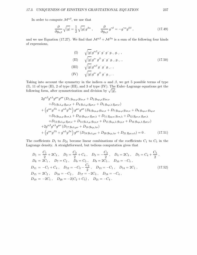
17.3. UNIQUENESS OF EINSTEIN’S GRAVITATIONAL EQUATION 237
In order to compute Mαβ , we use that
∂
∂gαβ
√|g| =
1
2
√|g| gβα ,
∂
∂gαβgγδ = −gγαgδβ , (17.49)
and we use Equation (17.27). We find that Mαβ + Mβα is a sum of the following four kindsof expressions,
(I)√|g| gαβg·· g·· g·· g··,· g··,· ,
(II)√|g| gα· gβ· g·· g·· g··,· g··,· , (17.50)
(III)√|g| gαβ g·· g·· g··,·· ,
(IV)√|g| gα· gβ· g·· g··,·· .
Taking into account the symmetry in the indices α and β, we get 5 possible terms of type(I), 11 of type (II), 2 of type (III), and 3 of type (IV). The Euler–Lagrange equations get thefollowing form, after symmetrization and division by
√|g|,
2gαβgκλgµνgρσ (D1 gκµ,ρ gλν,σ +D2 gκµ,ρ gλσ,ν
+D3 gκλ,ρ gµν,σ +D4 gκλ,ρ gµσ,ν +D5 gκρ,λ gµσ,ν)
+(gακgβλ + gαλgβκ
)gµνgρσ (D6 gκµ,ρ gλν,σ +D7 gκµ,ρ gλσ,ν +D8 gκµ,ν gλρ,σ
+D9 gκµ,ρ gνσ,λ +D10 gκµ,ν gρσ,λ +D11 gµρ,κ gνσ,λ +D12 gµν,κ gρσ,λ
+D13 gκλ,µ gρσ,ν +D14 gκλ,µ gνρ,σ +D15 gκµ,λ gνρ,σ +D16 gκµ,λ gρσ,ν)
+2gαβgκλgµν (D17 gκλ,µν +D18 gκµ,λν)
+(gακgβλ + gαλgβκ
)gµν (D19 gκλ,µν +D20 gκµ,λν +D21 gµν,κλ) = 0 . (17.51)
The coefficients D1 to D21 become linear combinations of the coefficients C1 to C5 in theLagrange density. A straightforward, but tedious computation gives that
D1 =C1
2+ 2C3 , D2 =
C2
2+C4 , D3 = −C3
2, D4 = 2C3 , D5 = C4 +
C5
2,
D6 = 2C1 , D7 = C2 , D8 = C5 , D9 = 2C5 , D10 = −C5 ,
D11 = −C1 +C4 , D12 = −C3 −C4
2, D13 = −C1 , D14 = 2C1 , (17.52)
D15 = 2C2 , D16 = −C2 , D17 = −2C3 , D18 = −C4 ,
D19 = −2C1 , D20 = −2(C2 + C5) , D21 = −C4 .
238 CHAPTER 17. LAGRANGE FORMALISM FOR THE GRAVITATIONAL FIELD
Problems
1. Use Noether’s theorem to derive a conservation law following from the general covarianceof the theory defined by the Lagrange “density” L′
G in Equation (17.34).
2. What conditions must be imposed on the coefficients D1 til D21 in Equation (17.51) tomake the equation generally covariant (i.e. invariant under general coordinate transfor-mations)?Do these conditions ensure that the equation can be derived from a Lagrange “density”(such as L′
G)?
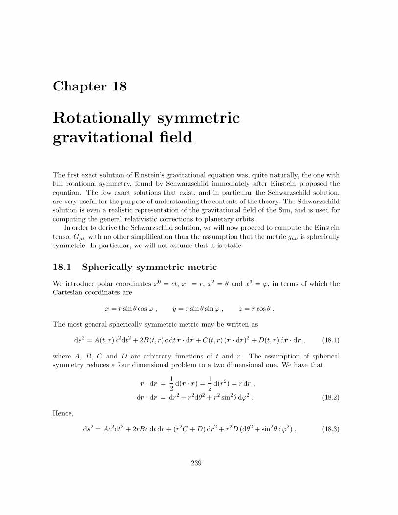
Chapter 18
Rotationally symmetricgravitational field
The first exact solution of Einstein’s gravitational equation was, quite naturally, the one withfull rotational symmetry, found by Schwarzschild immediately after Einstein proposed theequation. The few exact solutions that exist, and in particular the Schwarzschild solution,are very useful for the purpose of understanding the contents of the theory. The Schwarzschildsolution is even a realistic representation of the gravitational field of the Sun, and is used forcomputing the general relativistic corrections to planetary orbits.
In order to derive the Schwarzschild solution, we will now proceed to compute the Einsteintensor Gµν with no other simplification than the assumption that the metric gµν is sphericallysymmetric. In particular, we will not assume that it is static.
18.1 Spherically symmetric metric
We introduce polar coordinates x0 = ct, x1 = r, x2 = θ and x3 = ϕ, in terms of which theCartesian coordinates are
x = r sin θ cosϕ , y = r sin θ sinϕ , z = r cos θ .
The most general spherically symmetric metric may be written as
ds2 = A(t, r) c2dt2 + 2B(t, r) cdt r · dr +C(t, r) (r · dr)2 +D(t, r) dr · dr , (18.1)
where A, B, C and D are arbitrary functions of t and r. The assumption of sphericalsymmetry reduces a four dimensional problem to a two dimensional one. We have that
r · dr =1
2d(r · r) =
1
2d(r2) = r dr ,
dr · dr = dr2 + r2dθ2 + r2 sin2θ dϕ2 . (18.2)
Hence,
ds2 = Ac2dt2 + 2rBcdt dr + (r2C +D) dr2 + r2D (dθ2 + sin2θ dϕ2) , (18.3)
239

240 CHAPTER 18. ROTATIONALLY SYMMETRIC GRAVITATIONAL FIELD
or in matrix form,
gµν =
A rB 0 0rB r2C +D 0 00 0 r2D 00 0 0 r2D sin2θ
. (18.4)
The metric is diagonal, except that possibly g01 6= 0, and in addition we have g33 = g22 sin2θ.This is quite generally the form of a covariant tensor field of rank two, expressed in polarcoordinates, when it is symmetric under interchange of the two indices, and also rotationallysymmetric. Thus, spherical symmetry means that the Ricci tensor Rµν , the Einstein tensorGµν , and the energy momentum tensor Tµν must all be of a similar form.
We still have a certain freedom in choosing coordinates, and we may use it to simplifythe metric a little further. We assume that D < 0, and then we may introduce a new radialcoordinate
r = r√−D . (18.5)
Note that the relation between r and r is time dependent if D is time dependent, and thischange of coordinates removes any time dependence there might be in the angular componentsof the metric, g22 and g33. We get that
ds2 = Ac2dt2 + 2Bcdt dr + C dr2 − r2 (dθ2 + sin2θ dϕ2) , (18.6)
when we introduce new functions A = A(t, r), B = B(t, r) and C = C(t, r), given by A, B, Cand D. Note that the angular part of the metric determines the area of the two dimentionalsurface t = constant, r = constant to be 4πr 2. This expression for the area defines theparticular radial coordinate r.
We may make the metric completely diagonal by introducing a new time coordinate t,such that
cdt = E (Acdt+ B dr) . (18.7)
Here E = E(t, r) is an arbitrary integrating factor, such a factor exists because there are onlytwo independent variables t and r. In fact, all we have to do in order to solve Equation (18.7),with a function E(t, r) not specified beforehand, is to define a function t = t(t, r) such that tis constant on every integral curve in the (t, r) plane of the ordinary differential equation
Acdt+ B dr = 0 . (18.8)
Then we get that
ds2 =c2
AE2dt
2+
(C − B2
A
)dr 2 − r2 (dθ2 + sin2θ dϕ2) . (18.9)
Even now we have the freedom to choose another time coordinate which is an arbitraryfunction of t, without thereby destroying the diagonal form of the metric. We will use thisfreedom later on.
Let us now change our notation and write (t, r) for (t, r), and furthermore
ds2 = e2ac2dt2 − e2bdr2 − r2 (dθ2 + sin2θ dϕ2) , (18.10)
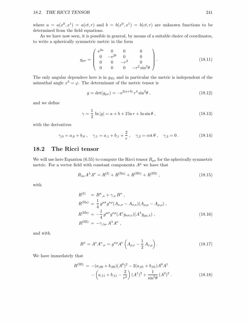
18.2. THE RICCI TENSOR 241
where a = a(x0, x1) = a(ct, r) and b = b(x0, x1) = b(ct, r) are unknown functions to bedetermined from the field equations.
As we have now seen, it is possible in general, by means of a suitable choice of coordinates,to write a spherically symmetric metric in the form
gµν =
e2a 0 0 00 −e2b 0 00 0 −r2 00 0 0 −r2 sin2θ
. (18.11)
The only angular dependece here is in g33, and in particular the metric is independent of theasimuthal angle x3 = ϕ. The determinant of the metric tensor is
g = det(gµν) = −e2(a+b) r4 sin2θ , (18.12)
and we define
γ =1
2ln |g| = a+ b+ 2 ln r + ln sin θ , (18.13)
with the derivatives
γ,0 = a,0 + b,0 , γ,1 = a,1 + b,1 +2
r, γ,2 = cot θ , γ,3 = 0 . (18.14)
18.2 The Ricci tensor
We will use here Equation (6.55) to compute the Ricci tensorRµν for the spherically symmetricmetric. For a vector field with constant componenta Aµ we have that
RλνAλAν = R(I) +R(IIa) +R(IIb) +R(III) , (18.15)
with
R(I) = Bκ,κ + γ,κB
κ ,
R(IIa) =1
4gµσgκρ(Aκ,σ −Aσ,κ)(Aρ,µ −Aµ,ρ) ,
R(IIb) = −1
4gµσgκρ(Aνgκσ,ν)(A
λgρµ,λ) , (18.16)
R(III) = −γ,λν AλAν ,
and with
Bκ = AνAκ;ν = gκρAν
(Aρ,ν − 1
2Aν,ρ
). (18.17)
We have immedately that
R(III) = −(a,00 + b,00)(A0)2 − 2(a,01 + b,01)A
0A1
−(a,11 + b,11 −
2
r2
)(A1)2 +
1
sin2θ(A2)2 . (18.18)
242 CHAPTER 18. ROTATIONALLY SYMMETRIC GRAVITATIONAL FIELD
Next,
Aµ = (A0, A1, A2, A3) = (e2aA0 , −e2bA1 , −r2A2 , −r2 sin2θ A3) . (18.19)
The partial derivatives of Aµ not vanishing identically are
A0,0 = 2a,0 e2aA0 , A0,1 = 2a,1 e2aA0 ,A1,0 = −2b,0 e2bA1 , A1,1 = −2b,1 e2bA1 ,A2,1 = −2rA2 ,A3,1 = −2r sin2θ A3 , A3,2 = −2r2 sin θ cos θ A3 .
(18.20)
This gives that
B0 = e−2a(
1
2A0A0,0 +A1
(A0,1 −
1
2A1,0
))
= a,0 (A0)2 + 2a,1A0A1 + b,0 e2(b−a) (A1)2 , (18.21)
B1 = −e−2b(A0(A1,0 −
1
2A0,1
)+
1
2A1A1,1 −
1
2A2A2,1 −
1
2A3A3,1
)
= a,1 e2(a−b) (A0)2 + 2b,0A0A1 + b,1 (A1)2 − r e−2b
((A2)2 + sin2θ (A3)2
),
B2 = − 1
r2
(A1A2,1 −
1
2A3A3,2
)=
2
rA1A2 − sin θ cos θ (A3)2 .
We do not bother to compute B3. In fact, it does not contribute to R(I), because thecoordinate x3 = ϕ is cyclic, that is, the metric does not depend on ϕ. We have that
R(I) =
(a,00 + (a,0)
2 + a,0 b,0 +
(a,11 + 3(a,1)
2 − a,1 b,1 +2a,1
r
)e2(a−b)
)(A0)2
+2
(a,01 + b,01 + a,0 a,1 + 2a,1 b,0 + b,0 b,1 +
2b,0r
)A0A1
+
((b,00 − a,0 b,0 + 3(b,0)
2)
e2(b−a) + b,11 + a,1 b,1 + (b,1)2 +
2b,1r
)(A1)2
− (3 + ra,1 − rb,1) e−2b((A2)2 + sin2θ (A3)2
)(18.22)
+2 cot θ
rA1A2 + (3 sin2θ − 2) (A3)2 .
We have further that
R(IIa) = −e−2(a+b)
2(A0,1 −A1,0)
2 +e−2b
2r2(A2,1)
2
+e−2b
2r2 sin2θ(A3,1)
2 +1
2r4 sin2θ(A3,2)
2 (18.23)
= −2(a,1)2 e2(a−b) (A0)2 − 4a,1 b,0A
0A1 − 2(b,0)2 e2(b−a) (A1)2
+2e−2b((A2)2 + sin2θ (A3)2
)+ 2cos2θ (A3)2 .
The metric tensor is diagonal, and for the diagonal elements we have that
Aνg00,ν = 2e2a (a,0A0 + a,1A
1) ,
Aνg11,ν = −2e2b (b,0A0 + b,1A
1) ,
Aνg22,ν = −2rA1 , (18.24)
Aνg33,ν = −2r sin2θ A1 − 2r2 sin θ cos θ A2 .
18.3. THE SCHWARZSCHILD METRIC 243
Furthermore,
R(IIb) = −e−4a
4(Aνg00,ν)
2 − e−4b
4(Aνg11,ν)2
− 1
4r4(Aνg22,ν)2 − 1
4r4 sin4θ(Aνg33,ν)2 . (18.25)
= −((a,0)2 + (b,0)
2) (A0)2 − 2(a,0 a,1 + b,0 b,1)A0A1
−(
(a,1)2 + (b,1)
2 +2
r2
)(A1)2 − 2 cot θ
rA1A2 − cot2θ (A2)2 .
The sum of the four contributions is
RλνAλAν =
(−b,00 − (b,0)
2 + a,0 b,0 +
(a,11 + (a,1)
2 − a,1 b,1 +2a,1
r
)e2(a−b)
)(A0)2
+
((b,00 + (b,0)
2 − a,0 b,0)
e2(b−a) − a,11 − (a,1)2 + a,1 b,1 +
2b,1r
)(A1)2
+4b,0r
A0A1 +(1 − (1 + ra,1 − rb,1) e−2b
) ((A2)2 + sin2θ (A3)2
). (18.26)
We may read the components Rλν of the Ricci tensor out of this formula. The scalar curvatureis
R = gλνRλν = e−2aR00 − e−2bR11 −R22
r2− R33
r2 sin2θ
= −2(b,00 + (b,0)2 − a,0 b,0) e−2a + 2(a,11 + (a,1)
2 − a,1 b,1) e−2b
− 2
r2
(1 − (1 + 2ra,1 − 2rb,1) e−2b
). (18.27)
Since the metric is diagonal, we have that Gλν = Rλν for λ 6= ν. The diagonal elements ofGλν are
G00 = R00 −e2a
2R =
e2a
r2
(1 + (2rb,1 − 1) e−2b
)=
e2a
r2∂
∂r
(r(1 − e−2b
)),
G11 = R11 +e2b
2R =
1
r2
(2ra,1 + 1 − e2b
), (18.28)
G22 = R22 +r2
2R
= −r2(b,00 + (b,0)2 − a,0 b,0) e−2a +
(r2(a,11 + (a,1)
2 − a,1 b,1) + r(a,1 − b,1))
e−2b ,
G33 = G22 sin2θ .
18.3 The Schwarzschild metric
The Schwarzschild metric is the spherically symmetric solution of the equation
Gλν = 0 , (18.29)
which is Einstein’s gravitational equation in vacuum. It is worth pointing out that we maychoose to restrict our solution of the equation to a limited interval in the radius r. Hence, the
244 CHAPTER 18. ROTATIONALLY SYMMETRIC GRAVITATIONAL FIELD
Schwarzschild metric may be interpreted quite generally as, for example, the gravitationalfield outside an arbitrary spherically symmetric mass distribution.
The equation G01 = 2b,0/r = 0 means that b is constant in time, b = b(r). Then theequation G00 = 0 has the solution
e−2b = 1 − RM
r, (18.30)
where RM is a time independent integration constant with the dimension of length. Theindex “M” is written here to suggest that RM is somehow related to a gravitational mass Mwhich is the source of the field. Here and now this is a suspicion, to be confirmed shortly.
The two equations G00 = 0 and G11 = 0 together give that
a,1 + b,1 =r
2
(e2(b−a)G00 +G11
)= 0 , (18.31)
which means that a+ b = f(t) for an arbitrary function f(t), so that
e2a dt2 = e−2be2f(t) dt2 . (18.32)
Without any loss of generality we may assume that f(t) = 0, since otherwise we may simplyreplace t by a new time coordinate t such that
dt = ef(t) dt . (18.33)
Thus we get that
e2a = e−2b = 1 − RM
r. (18.34)
This solves the three equations G00 = G11 = G01 = 0. The two remaining equations,G22 = G33 = 0, reduce to one, G22 = 0, reducing further to the equation
ra,11 + (ra,1 + 1)(a,1 − b,1) = 0 . (18.35)
It holds identically with the above expressions for a and b.
Physical interpretation
In order to interpret the integration constant RM we let r become large, because we knowthat g00 = e2a is then given by Newton’s gravitational potensial φ as
e2a = 1 +2φ
c2= 1 − 2GM
c2r, (18.36)
where G is Newton’s gravitational constant, and M is a constant corresponding to the grav-itational mass in Newton’s theory. We see that
RM =2GM
c2. (18.37)
18.4. PLANETARY ORBITS 245
This is a characteristic length defined by the mass M , called the gravitational radius, or theSchwarzschild radius.
The Earth, for example, has a mass of 6.0× 1024 kg and a gravitational radius of 8.9 mm.The Sun has a mass of 2.0 × 1030 kg and a gravitational radius of 3.0 km.
Thus, the Schwarzschild metric having the mass M as its source is
ds2 =
(1 − 2GM
c2r
)c2dt2 − dr2
1 − 2GMc2r
− r2(dθ2 + sin2θ dϕ2) . (18.38)
It describes the gravitational field in vacuum outside an arbitrary spherically symmetric massdistribution with a total gravitational mass M . Inside the mass distribution the metric ismodified and differs from the Schwarzschild metric, but on the outside the metric is uniquelygiven, apart from the freedom we always have to choose space and time coordinates. Thisresult, which is proved by our present computation, that the metric is uniquely given whenthe source is spherically symmetric and the total mass is given, is known as Birkhoff’s the-orem. Note that the proof is based on the implicit assumption that the metric must bespherically symmetric when the mass distribution is. Birkhoff’s theorem corresponds to theresult demonstrated by Newton, that the gravitational field outside a spherically symmetricmass distribution is the same as if all the mass were collected at the centre.
The Schwarzschild metric is static, as seen from the coordinate system we have chosen,and this is true regardless of whether the source of the field is static, as long as all the motionsmaintain the spherical symmetry. This means, first of all, that the total gravitational massM is concerved.
Furthermore, since a static field can not describe radiation, and since there exist no othersolutions, it means that a spherically symmetric mass distribution is incapable of emittinggravitational radiation. Like electromagnetic radiation, gravitational radiation can not bemonopole radiation. Note that if energy is radiated by other means than by gravitationalradiation, e.g. electromagnetically, then there is no longer vacuum outside the mass distribu-tion, and we have Gµν = κTµν 6= 0. Then the gravitational field is modified, and the metricis no longer the Schwarzschild metric.
18.4 Planetary orbits
The Schwarzschild metric ought to be a good approximation to the gravitational field of theSun, so that we may use it in order to compute the orbits of the planets. The simplestapproach is to derive the equations of motion directly from the variational principle, withoutcomputing explicitly the connection coefficients. Our task is then to extremalize the actionintegral S = −mc ∫ duw, where m is the mass of the planet, u is an arbitrary parameteralong the orbit, and
w =ds
du=
√√√√(
1 − RM
r
)c2t2 − r2
1 − RMr
− r2(θ2 + sin2θ ϕ2)
=
√(1 − RM
r
)c2t2 − |r|2 − RM (r · r)2
r2(r −RM ). (18.39)
246 CHAPTER 18. ROTATIONALLY SYMMETRIC GRAVITATIONAL FIELD
We write t = dt/du, r = dr/du, etc..This problem obviously has enough symmetry to be exactly solvable, although it may be
impossible to express the general solution in terms of elementary functions. First, w is notexplicitly dependent on the “coordinate” t, and this fact implies a conservation law for thecanonically conjugate momentum, which has a certain right to the name of “energy”. Second,w is rotationally invariant, which means that the angular momentum,
L = −mc r × ∂w
∂r=mc
wr × r , (18.40)
is conserved. Since r · L = 0, it follows that the orbit lies in a plane through the origin,perpendicular to the constant vector L. Therefore we may choose our coordinate system insuch a way that the orbital plane has the equation θ = π/2.
For the three variables t, θ and ϕ we get the explicit Euler–Lagrange equations
0 =d
du
(∂w
∂t
)=
d
du
(1
w
(1 − RM
r
)c2t
),
0 =d
du
(∂w
∂θ
)− ∂w
∂θ= − d
du
(r2θ
w
)+r2 sin θ cos θ ϕ2
w, (18.41)
0 =d
du
(∂w
∂ϕ
)= − d
du
(r2 sin2θ ϕ
w
).
The first equation has the solution
dt
ds=
t
w=
A
c(1 − RM
r
) , (18.42)
where A is a dimensionless integration constant. The quantity
−mc ∂w∂t
= −mc2A (18.43)
is the momentum canonically conjugate to t, so that mc2A is to be interpreted as the energy.The third equation has the solution
dϕ
ds=ϕ
w=
BRM
r2 sin2θ, (18.44)
where B is another dimensionless integration constant. B is proportional to the angular mo-mentum about the z axis, Lz, which is the canonically conjugate momentum of the asimuthalangle ϕ,
Lz = −mc ∂w∂ϕ
= mcRMB . (18.45)
We see that we may solve the second equation by setting θ = π/2. As already mentioned,every solution of the equation of motion in the Schwarzschild metric may be described in thisway, by a suitable choice of coordinates.
18.4. PLANETARY ORBITS 247
Strangely enough, there is no need to write out the Euler–Lagrange equation for r, becausewe find a first integral of it simply by squaring w, and substituting the above expressions fort and ϕ, as well as θ = π/2. We get that
w2 =w2A2
1 − RMr
− r2
1 − RMr
− w2B2RM2
r2. (18.46)
Here we may introduce the dimensionless variable ψ = RM/r, and write
r = ϕdr
dϕ=wBRM
r2dr
dϕ= −wB dψ
dϕ. (18.47)
The result is the following equation for ψ,
(dψ
dϕ
)2
=A2 − 1 + ψ
B2− ψ2 + ψ3 . (18.48)
By differentiating this equation we obtain a second order differential equation for ψ,
d2ψ
dϕ2=
1
2B2− ψ +
3
2ψ2 . (18.49)
Comparison with Newton’s theory
Newton’s equations of motion for a planet of mass m in the equatorial plane θ = π/2 followfrom the conservation of angular momentum
Lz = mr2dϕ
dt(18.50)
and energy
E =m
2
((dr
dt
)2
+ r2(
dϕ
dt
)2)− GmM
r. (18.51)
We may introduce the same dimensionless variable ψ = RM/r, and write the energy equationin the dimensionless form
2E
mc2=
1
c2
(dϕ
dt
)2((
dr
dϕ
)2
+ r2)− 2GM
c2r
=
(Lz
mcr2
)2((
dr
dϕ
)2
+ r2)− RM
r(18.52)
=
(Lz
mcRM
)2((
dψ
dϕ
)2
+ ψ2
)− ψ .
248 CHAPTER 18. ROTATIONALLY SYMMETRIC GRAVITATIONAL FIELD
Or equivalently,
(dψ
dϕ
)2
=2mERM
2
Lz2 +
(mcRM
Lz
)2
ψ − ψ2 . (18.53)
This non-relativistic equation has the same form as equation (18.48), except for the ab-sence of the term ψ3. By comparing the two equations we see what the two integrationconstants A and B correspond to in the non-relativistic limit,
B =Lz
mcRM, A =
√
1 +2E
mc2. (18.54)
The dimensionless variable ψ = RM/r is very small for all the planets in the solar system,in fact ψ < 10−7, since RM = 3 km for the Sun, whereas r ≈ 5 × 10⁷ km for the inner-most planet Mercury. Therefore the extra term ψ3 in Equation (18.48) is always a smallperturbation.
Approximate solution
By simply neglecting the last, quadratic, term in Equation (18.49) we find the non-relativisticsolution,
ψ =1 + e cos(ϕ− ϕ0)
2B2, (18.55)
where e and ϕ0 are integration constants. We may always choose e ≥ 0. Equation (18.48)without the term ψ3 gives the following relation between the integration constants A, B, ande,
e2 = 4B2(A2 − 1) + 1 . (18.56)
Equation (18.55) is the equation for a conic section with one focus at the origin, and witheccentricity e: a circle if e = 0, an ellipse if 0 < e < 1, a parabola if e = 1, or a hyperbola ife > 1.
To see this a little more explicitly, we may define
x = −r cos(ϕ− ϕ0) , y = r sin(ϕ− ϕ0) , (18.57)
such that the equation takes the form 2B2RM = r − ex. The equation for an ellipse witheccentricity e, one focus at the origin, and the second focus at (x, y) = (2ea, 0), where a > 0,is
r +√
(x− 2ea)2 + y2 = 2a . (18.58)
Here a is the major half axis of the ellipse. The equation may be rewritten as follows,
(x− 2ea)2 + y2 = (2a− r)2 , (18.59)
or further as
(1 − e2)a = r − ex . (18.60)
18.4. PLANETARY ORBITS 249
Thus, the major half axis is, when we use Equation (18.56),
a =2B2RM
1 − e2=
RM
2(1 −A2)=
GM
c2(1 −A2). (18.61)
That point of the orbit where r is minimal, and hence ψ maximal, is called perihelion.Equation (18.55) describes an orbit with its perihelion at ϕ = ϕ0. If the orbit is an ellipse(or a circle), all values are allowed for the angle ϕ, and the orbit is a closed curve, since theperihelion angle after n periods is
ϕn = ϕ0 + 2nπ . (18.62)
The most accurate way to linearize Equation (18.49), however, is not to neglect the termψ2 altogether, but rather to write ψ = ψ0 +∆ψ, with ψ0 = RM/r0 constant, and then neglect(∆ψ)2. This gives a slightly different approximate equation linear in ∆ψ,
d2
dϕ2∆ψ =
1
2B2− ψ0 +
3
2ψ0
2 − (1 − 3ψ0)∆ψ . (18.63)
We choose ψ0 as a solution of the equation
1
2B2− ψ0 +
3
2ψ0
2 = 0 . (18.64)
Or as a more practical approach, we choose first ψ0 and let this equation determine theintegration constant B. That gives the solution
∆ψ = eψ0 cos(√
1 − 3ψ0 (ϕ− ϕ0)). (18.65)
According to this more accurate solution, the perihelion angle after n periods is
ϕn = ϕ0 +2nπ√
1 − 3ψ0= ϕ0 + 2nπ + 3nπψ0 . (18.66)
Thus, every time the planet completes a full circuit around the Sun, the perihelion pointmoves a small angle
∆ϕ = 3πψ0 =3πRM
r0=
6πGM
c2r0. (18.67)
In the solar system, the advance in the perihelion point is largest and most easily observ-able for Mercury, because it is the planet closest to the Sun, and because its orbit is rathereccentric. The solar mass is M = 1.989 × 1030 kg. Mercury has an orbital period of 87.969days, and a mean distance from the Sun of rm = 5.791×10¹⁰ m. However, the quantity neededhere is the mean inverse distance, ψ0 = RM/r0. The eccentricity is e = 0.205 63, which meansthat the distance from the Sun varies between r1 = r0/(1+e) = 0.8294 r0 and r2 = r0/(1−e) =1.2589 r0. Thus, the mean distance is rm = 1.0442 r0 , and hence r0 = 5.546× 10¹⁰ m. During100 Earth years, or 36 525 days, Mercury completes 36 525/87.969 = 415.20 turns around the
250 CHAPTER 18. ROTATIONALLY SYMMETRIC GRAVITATIONAL FIELD
Sun, and its accumulated perihelion advance due to the general relativistic correction to itsequation of motion is
415.20∆ϕ = 42.98′′ . (18.68)
The observed perihelion advance of Mercury during one hundred years amounts to
5599.74′′ ± 0.41′′ (18.69)
according to data from 1947. This figure has to be corrected for the precession of the rotationaxis of the Earth, with a period of 26 000 years. The precession implies that the tropical year,which is the year followed by our calendar, is 20 minutes and 24 seconds shorter than thesiderial year, which is measured relative to the fixed stars, and which is the relevant timereckoning for measuring the perihelion advance of Mercury. This contribution to the directlyobserved perihelion advance was in 1947 computed to be
5025.65′′ ± 0.50′′(≈ 2π
100 years
26 000 years
)(18.70)
per one hundred years. Another contribution, due to the gravitational influence of the otherplanets, mainly Jupiter, was computed to be 531.54′′ ± 0, 68′′. The residual angle of 42.56′′ ±0, 94′′ is compatible with the prediction made by the general theory of relativity. One quantitywhich used to be uncertain, and which influences the perihelion advance, is the oblateness ofthe interior of the Sun due to rotation.
18.5 Generalizations of the Schwarzschild metric
The Reissner–Nordstrom metric
Not long after Schwarzschild found his solution it was generalized by Reissner and Nordstromto the case when there is also a spherically symmetric electric field, but no electric charge inthe region where we solve the equation. The metric is still almost as simple,
ds2 =
(1 − RM
r+RQ
2
r2
)c2dt2 − dr2
1 − RMr +
RQ2
r2
− r2(dθ2 + sin2θ dϕ2) . (18.71)
The electric field is radial, and the radial component is
Er = cF01 = −cF 01 =Q
4πǫ0 r2. (18.72)
Using Gauss’s law on a spherical surface of constant r, and remembering that the angularpart of the metric is the same as in Euclidean space, we see that the constant Q is simply the
18.5. GENERALIZATIONS OF THE SCHWARZSCHILD METRIC 251
total electric charge inside the surface. The new constant RQ in the metric is a characteristiclength given by the charge Q,
RQ2 =
GQ2
4πǫ0 c4. (18.73)
Using (without any good justification) the usual relation between the metric gµν andNewton’s gravitational potential φ, that g00 ≈ 1 + (2φ/c2), we have here that
φ ≈ −RM c2
2r+RQ
2c2
2r2. (18.74)
Then the gravitational force on a mass m at a distance r is
−m dφ
dr≈ −mRM c2
2r2+mRQ
2c2
r3. (18.75)
By this formula, the gravitational force is repelling for
r <2RQ
2
RM=
Q2
4πǫ0Mc2. (18.76)
This surprising resultat may be understood as follows. The electric field has an energy densityspread out all over space, and diverging in the limit r → 0 so strongly that the total energyof the electric field, from r = 0 to r = ∞, becomes infinite. In order to make the totalgravitational mass M finite, we must compensate the infinite field energy by another infiniteand negative point mass at the origin, and it is this negative mass which is felt when we getclose enough.
It may be interesting to compare the two characteristic lengths RM and RQ e.g. for anelectron, with Q = −|e|. The gravitational length of the electron is
RM =2Gme
c2= 1.4 × 10−57 m , (18.77)
whereas the “charge length” is
RQ =
√RM re
2= 1.4 × 10−36 m = 1021 RM . (18.78)
Here re = Q2/(4πǫ0 mec2) = 2.8 × 10⁻¹⁵ m is the classical electron radius.
The Kerr–Newman metric
If the mass which is the source of the gravitational field rotates, then the field no longerhas the full rotational symmetry, but has only an axial symmetry. The generalization of theSchwarzschild solution to this case is rather more complicated, it was found in 1963, by Kerr.Newman found the corresponding solution with an electromagnetic field.
252 CHAPTER 18. ROTATIONALLY SYMMETRIC GRAVITATIONAL FIELD
18.6 Black and white holes
In the extreme case where all the gravitational mass M is concentrated inside a radius smallerthan the Schwarzschild radius RM , the Schwarzschild metric describes a so called black hole.The idea that such objects might exist is actually much older than Einstein and Schwarzschild.An Englishman, John Michell, and a Frenchman, Laplace, speculated already two hundredyears ago that there might exist planets or stars with such strong gravitational fields thatthe escape velocity exceeds the speed of light c. In Newton’s gravitational theory the escapevelocity v0 at a distance r from the mass M is given by the relation
v02
2− GM
r= 0 . (18.79)
This is the condition that the kinetic plus potential energy of a particle is exactly zero, so thatthe particle has just enough kinetic energy to escape to r = ∞. By accident, the Schwarzschildradius RM is precisely the radius where the non-relativistic escape velocity v0 equals the speedof light.
The Schwarzschild metric is singular at the Schwarzschild radius, and t and r exchangetheir roles inside r = RM , in such a way that r becomes a time coordinate and t a spacecoordinate! This so called “Schwarzschild singularity” at r = RM caused much confusion,until it became clear that it is not really a singularity of the spacetime geometry, it is only asingularity of the metric appearing because we have chosen singular coordinates. The metricsingularity at r = RM is no more serious than the singularities at the North Pole θ = 0 andthe South Pole θ = π in polar coordinates. Spacetime itself with the Schwarzschild metric isno more singular at r = RM than the surface of a sphere is singular at θ = 0 or θ = π. Oneindication that the geometry is nonsingular is perhaps the fact that the determinant of themetric is nonsingular and nonzero in the limit r → RM .
The significance of the gravitational radius r = RM is that it is a horizon. It is impossibleto observe from the outside anything beyond the horizon. Everything crossing this radiusfrom the outside, sails out of sight of any observer staying outside r = RM . In particular, aradial light signal starting at r = RM in the outward direction will stay forever at the samedistance r = RM from the origin. And a light signal starting inside r = RM , in any directionwhatsoever, will fall towards r = 0.
Nonsingular coordinates
The time coordinate t may be identified as the source of the singularity in the Schwarzschildmetric in its original form. The simplest way to transform away the singularity is to introducea new time coordinate
v = ct+ r +RM ln
∣∣∣∣r −RM
RM
∣∣∣∣ . (18.80)
This gives that
cdt = dv − r dr
r −RM, (18.81)
and hence,
ds2 =
(1 − RM
r
)dv2 − 2 dv dr − r2(dθ2 + sin2θ dϕ2) . (18.82)
18.6. BLACK AND WHITE HOLES 253
This is known as the Eddington–Finkelstein form of the Schwarzschild metric, and it is clearlyas simple as it can be made. The price we pay for obtaining a non-singular form of the metricis to introduce an off-diagonal term dv dr, which means that the time reversal symmetry ofthe metric is no longer explicit.
The physical meaning of the new time coordinate is that v = constant is the equation ofan incoming radial light signal. If we introduce
v′ = ct− r −RM ln
∣∣∣∣r −RM
RM
∣∣∣∣ (18.83)
instead of v, then v′ = constant is the equation of an outgoing radial light signal, and thetime reversal transformation t 7→ −t corresponds to v 7→ −v′.
Another set of coordinates that are nonsingular at r = RM are the Kruskal–Szekerescoordinates u and v, replacing r and t and defined by the relations
u2 − v2 = f(r) =
(r
RM− 1
)er/RM ,
v
u= g(t) =
tanh(ct/(2RM )) for r > RM ,coth(ct/(2RM )) for r < RM .
(18.84)
This definition is consistent, since it gives that
u2 =f
1 − g2≥ 0 , v2 =
fg2
1 − g2≥ 0 . (18.85)
Writing f ′ = df/dr and g = dg/dt, we have that
2udu− 2v dv = df = f ′ dr ,dv
u− v du
u2= dg = g dt . (18.86)
Substituting for dr and dt in the line element ds2, we find after some manipulations that
ds2 =4RM
3
re−r/RM (dv2 − du2) − r2(dθ2 + sin2θ dϕ2) , (18.87)
both for r > RM and for r < RM . Again the apparent singularity at r = RM is eliminated.On the other hand, there is no doubt that the metric is singular at the origin, r = 0.
This singularity can not be transformed away. That such a singularity inside a closed horizonis inevitable, under certain “reasonable” assumptions on the energy momentum tensor, wasproved by Roger Penrose in 1965.
The Kruskal–Szekeres coordinates give an illuminating picture of the geometry of space-time with the Schwarzschild metric, when we imagine that the source is a point mass lyingat rest at the origin. See Figure 18.1. Perhaps the most interesting phenomenon is that thewhole spacetime is doubled. In fact, to one point (r, t) in space and time there correspondstwo values (u, v) and (−u,−v) of the new coordinates. One way out of this dilemma mightbe to say that (u, v) and (−u,−v) describe the same point in spacetime, but if we do so, wecreate confusion about the concept of causality, as we shall see. The most direct interpreta-tion is to say that (u, v) and (−u,−v) represent two different points in space and time, eventhough it means that we make spacetime twice as big.
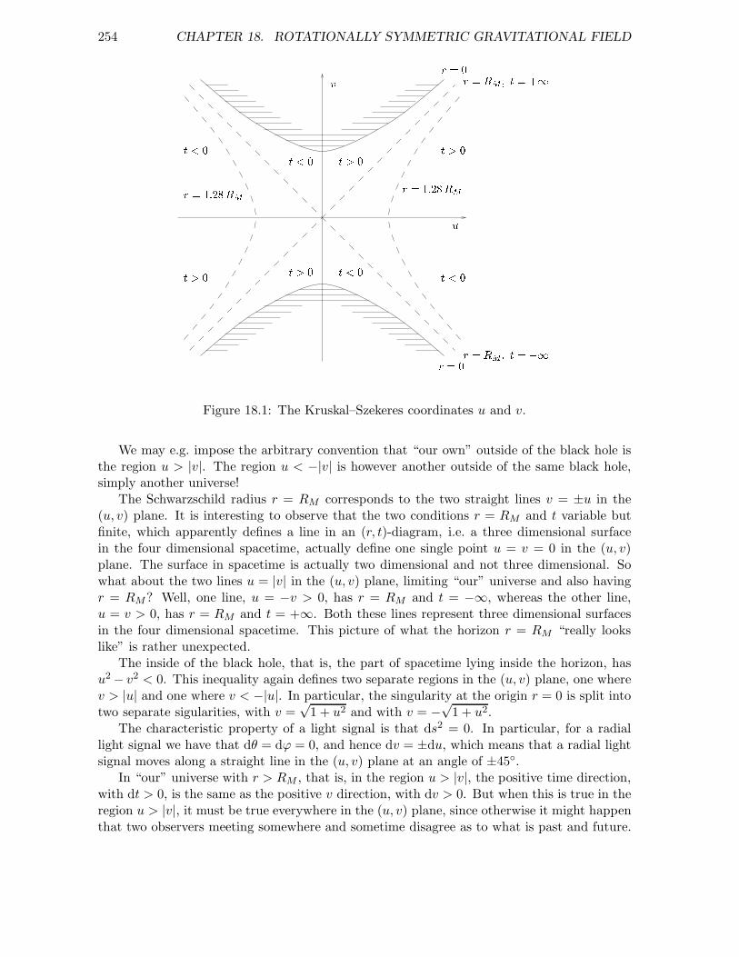
254 CHAPTER 18. ROTATIONALLY SYMMETRIC GRAVITATIONAL FIELD
r = RM ; t = 1
r = 0
r = 0
r = RM ; t = +1t < 0t > 0 t < 0
t > 0r = 1:28RMuv
t < 0t > 0
t > 0t < 0r = 1:28RM
Figure 18.1: The Kruskal–Szekeres coordinates u and v.
We may e.g. impose the arbitrary convention that “our own” outside of the black hole isthe region u > |v|. The region u < −|v| is however another outside of the same black hole,simply another universe!
The Schwarzschild radius r = RM corresponds to the two straight lines v = ±u in the(u, v) plane. It is interesting to observe that the two conditions r = RM and t variable butfinite, which apparently defines a line in an (r, t)-diagram, i.e. a three dimensional surfacein the four dimensional spacetime, actually define one single point u = v = 0 in the (u, v)plane. The surface in spacetime is actually two dimensional and not three dimensional. Sowhat about the two lines u = |v| in the (u, v) plane, limiting “our” universe and also havingr = RM? Well, one line, u = −v > 0, has r = RM and t = −∞, whereas the other line,u = v > 0, has r = RM and t = +∞. Both these lines represent three dimensional surfacesin the four dimensional spacetime. This picture of what the horizon r = RM “really lookslike” is rather unexpected.
The inside of the black hole, that is, the part of spacetime lying inside the horizon, hasu2 − v2 < 0. This inequality again defines two separate regions in the (u, v) plane, one wherev > |u| and one where v < −|u|. In particular, the singularity at the origin r = 0 is split intotwo separate sigularities, with v =
√1 + u2 and with v = −
√1 + u2.
The characteristic property of a light signal is that ds2 = 0. In particular, for a radiallight signal we have that dθ = dϕ = 0, and hence dv = ±du, which means that a radial lightsignal moves along a straight line in the (u, v) plane at an angle of ±45.
In “our” universe with r > RM , that is, in the region u > |v|, the positive time direction,with dt > 0, is the same as the positive v direction, with dv > 0. But when this is true in theregion u > |v|, it must be true everywhere in the (u, v) plane, since otherwise it might happenthat two observers meeting somewhere and sometime disagree as to what is past and future.
18.6. BLACK AND WHITE HOLES 255
It seems a reasonable requirement that the concepts of past and future should have a uniquemeaning. But it is violated if we try to identify the opposite points (u, v) and (−u,−v), sincethat means identifying dv at the point (u, v) with −dv at the point (−u,−v).
That positive v direction represents future, means in particular that the singularity atv =
√1 + u2 is a future singularity, a black hole, whereas the singularity at v = −
√1 + u2 is
a past singularity, a white hole. Nothing can emerge from the future singularity, and nothingcan fall into the past singularity. Nothing falling in through the Schwarzschild radius, whichmeans crossing the line v = |u|, can avoid falling into the future singularity. And similarly,nothing can come out through the Schwarzschild radius, meaning that it passes the linev = −|u|, if it has not first come out of the past singularity.
Gravitational collapse
The Sun and other stars may burn for millions or billions of years thanks to the energyliberated when protons and other light atomic nuclei fusion into heavier nuclei. Matter insidean ordinary star is almost an ideal gas, even though the high pressures may compress it intodensities many times the density of a heavy metal like gold under laboratory conditions onEarth. The luminosity is very nearly constant during most of the lifetime of a star, becausethere exists a stable equilibrium between the gravitational force compressing the gas, and thegas pressure opposing the compression. In the most massive stars also the radiation pressuredue to the gas of photons plays a role.
The equilibrium is stable because a small local compression of the gas would increaseboth the temperature and the pressure, as described by the equation of state. In addition,inside the core where energy production by nuclear processes takes place, compression wouldincrease the rate of energy production, thereby heating the gas and raising the pressure evenmore. Yet another effect would be an increase in radiation pressure, because the matter wouldbecome more opaque. A small expansion would have the opposite effects, thus the effects ofeither compression or expansion tend to restore the same equilibrium conditions as before.
When the star has spent its nuclear fuel, it starts cooling because the energy keeps ra-diating away from its surface, and as a result, the gravitational forces compress it. Thecompression leads to heating of the gas, and if the star is sufficiently massive, it may reachthe threshold temperature of another nuclear fusion process. However, in the end all possiblefusion processes will be completed, and the only effect which may stop the compression, inthe end, is the circumstance that the particles bulding up the matter inside the star, arefermions. N electrons, for example, can not be compressed into a phase space volume smallerthan Nh3/2, where h is Planck’s constant, and the factor 2 appears because every electronmay have 2 spin states. Thus, the N electrons will fill a certain minimal volume in threedimensional space, inversely proportional to the volume available in momentum space. Whenthe electron gas is compressed as much, it is said to be degenerate, and the star can notcontract any more. It has then become a white dwarf star.
When the Sun reaches the white dwarf stage, it will have a radius of about one per centof its present radius, or roughly the radius of the Earth. Several hundred stars have beenidentified as white dwarfs, and there exist several thousand “candidates”. The closest whitedwarf is Sirius B, orbiting Sirius A, with an orbital period of 50 years. Sirius A and B areamong the very closest stars, at a distance of only 9 light years, and Sirius A is the brightestof all the stars in the sky, with the exception of the Sun.
When a star contracts, after having spent its nuclear fuel, the gas is heated more the
256 CHAPTER 18. ROTATIONALLY SYMMETRIC GRAVITATIONAL FIELD
larger mass the star has, and as a result the available volume in momentum space increases.This means that the density of a white dwarf is larger the larger its mass, and actually somuch larger that its radius is smaller the larger its mass. There exists a mass, about 1.4times the solar mass, at which the radius of a white dwarf would be zero, or more precisely,the central density of the star would become infinite. This mass is called the Chandrasekharmass, and it is an upper limit for the mass of a white dwarf star. If a star has a larger mass,the pressure from the degenerate electron gas is insufficient to stop the contraction.
When a star of mass exceding the Chandrasekhar mass contracts, the electrons will geta high enough energy that they start reacting with the protons to produce neutrons andneutrinoes. The neutrinoes simply escape from the star, bringing with them a not negligi-ble amount of energy, whereas the neutrons stay. If the mass is not too much larger thanthe Chandrasekhar mass, the result may be a neutron star, consisting mostly of degenerateneutrons. A neutron star of the same mass as the Sun would have a radius of about 10 km,which is only about three times the gravitational radius, and a density around 1015 times thedensity of water, about the same deneity as in an atomic nucleus. A neutron star is essentiallya giant atomic nucleus.
Neutron stars are observed as pulsars, and more than a thousand are now known. Theyare very small, by stellar measures, and hence radiate little light from their surfaces, eventhough they are hot. However, they radiate in all parts of the electromagnetic spectrum, fromradio waves to X rays and even γ rays, mostly in brief pulses, many pulses per second. Thepulse period of one pulsar is very nearly constant, except for “glitches” from time to time, atwhich the period suddenly increases in small jumps.
The pulsing is believed to result from the rotation of the neutron star, with a rotationperiod of a small fraction of a second. The enormously strong magnetic field is not parallel tothe rotation axis, and the rotating magnetic field will accelerate charged particles, especiallyelectron, which emit electromagnetic radiation.
There exists an upper limit to the mass of a neutron star, corresponding to the Chan-drasekhar mass. This upper limit is not very accurately known, because the exact equationof state is not very well known at the high densities found inside a neutron star, but it is cer-tainly no more than a few solar masses, and probably no more than about two solar masses.A more massive star has only two alternatives open, as far as is known: it must either shedenough mass maybe in a supernova explosion, that it gets below the critical limit, or it mustcollapse into a black hole.
A black hole formed by gravitational collapse of a mass distribution without any singu-larities does not correpond directly to a black hole as described by the Schwarzschild metric.Apart from the fact that in practise it could never be exactly spherically symmetric, themost important difference is that it has only a future singularity, and no past singularity.Fortunately, this means that the extra universe contained in the Schwarzschild metric is notpresent.
The only observable objects left as remainders of a star falling inside its own Schwarzschildhorizon, will be the gravitational field, and possibly an electromagnetic field. The gravita-tional field will symmetrize itself by gravitational radiation, most of which will disappear intothe hole, in such a way that the field left will be described to a good approximation by theKerr–Newman solution of the combined Einstein’s and Maxwell’s equations. Such a blackhole is completely described by only three parameters, mass, spin and electric charge. Thisresult was formulated by Wheeler in the following way,
18.7. HAWKING RADIATION, OR GREY, RED AND BLUE HOLES 257
“Black holes have no hair”.
An important clue when looking for black holes, and attempting to distinguish them fromordinary stars, neutron stars and other sources of electromagnetic radiation, is that theypossess a mechanism for converting mass into radiation which is much more efficient thanother known mechanisms. The fusion of atomic nuclei inside stars is capable of convertingless than one per mille of the mass into radiation energy, an important reason for the limitationbeing that baryon number is conserved: protons and neutrons may be converted into eachother, but never destroyed, at least not in ordinary nuclear reactions. On the other hand, itis estimated that when matter falls into a black hole, as much as 20% of the rest energy ofthe mass may be reradiated. In a sense, baryon number is not conserved in such a process,because the baryons disappear into the black hole, and the radiated energy comes from thegravitational potential energy converted into kinetic energy when the matter is falling in.
There are two cases where astronomers believe they see the signatures of black holes. Onekind of black holes are those that are formed when the most massive stars burn out andcollapse in supernova explosions. A small number of likely black hole candidates of this kindhave been identified. They are members of double star systems, and are observed, by Kepler’sthird law relating the sum of the masses of the two stars to the orbital period and the distancebetween them, to have masses several times the solar mass. Furthermore, they are all sourcesof X-ray radiation, implying that they have high surface temperatures, but at ther same timethey are not directly visible, implying that they must be very compact. Presumably theX-ray radiation is produced when mass transferred from the other star accumulates into aflat accretion disc and eventually falls into the black hole.
Much more massive black holes seem to exist at the centres of many galaxies, perhaps evenin all galaxies, including our own Milky Way galaxy. Especially quasars (“quasi stellar”, i.e.starlike, objects) seem to produce enormous amounts of radiation energy from comparativelyvery small volumes, which it is hard to explain by any other known mechanism than that ofmatter falling into a black hole. There are indications that the quasars are the galactic nucleiof young galaxies.
18.7 Hawking radiation, or grey, red and blue holes
A spherically symmetric black hole has a surface area of
A = 4πRM2 =
16πG2M2
c4, (18.88)
since the angular part of the Schwarzschild metric is the same as in flat space, in polarcoordinates, r2(dθ2 + sin2θ dϕ2). More generally, the horizon around a (stationary) blackhole has always a well defined area, even if it is not the surface of a sphere.
Stephen Hawking proved in 1971 a result which resembles the second law of thermody-namics, and which is therefore called the second law of black hole dynamics:
The total area of a black hole can never decrease.
258 CHAPTER 18. ROTATIONALLY SYMMETRIC GRAVITATIONAL FIELD
For example, if two black holes of masses M1 and M2 collide and merge into one, the followinginequality must hold for the mass M of the resulting single black hole,
M2 ≥M12 +M2
2 . (18.89)
This sets an upper limit to the amount of energy that may be radiated during the collision,in the form of gravitational radiation or other types of radiation.
This law, like the second law of thermodynamics, breaks time reversal invariance, andone may ask how that is possible, since it is proved from laws that are invariant under timereversal. The point is that it is valid for black holes, which are future singularities, formedfrom non-singular mass distributions by gravitational collapse. For white holes, formed in thebig bang when the Universe was born, and disappearing after a finite time, there must bea corresponding law saying that the sum of areas of white hole horizons can never increase.White holes are problematic for theoretical reasons, and the simplest assumption is thatthey do not exist. They have not yet been observed, and it is also somewhat unclear whatproperties they should have if they do exist.
It would seem tempting to postulate that the second law of black hole dynamics is nothingbut another example of the second law of thermodynamics. This would be the case if a blackhole has an entropy proportional to its area. Jacob Bekenstein proposed to take this ideaseriously, but met opposition from most other experts, not least from Hawking. One problemis that a black hole having entropy must also have a finite temperature, and hence emittemperature radiation. Thus, it is not black, it has one or another of the colours of therainbow, depending on its temperature.
However, Hawking soon turned around and accepted the idea of black hole entropy and fi-nite temperature, after he followed up an idea of Yakov Zel’dovich and Alexander Starobinsky,calculating a quantum mechanical process in which spontaneous particle radiation is emittedfrom a black hole. He convinced himself that the effect is real, and the spectral distributionwhich he calculated was precisely the one coming from black body radiation of the temper-ature a black hole must have if its entropy is proportional to its area. Thus, two classicaltheories in combination, the general theory of relativity and termodynamics, led to the ideaof temperature radiation from a black hole, which is a quantum mechanical effect.
The Hawking radiation from a black hole correspond to its entropy being
S =kBc
3
4hGA =
4πkBGM2
hc=
4πkBM2
mP2
. (18.90)
Here Newton’s gravitational constant G, Planck’s constant h = 2πh, Boltzmann’s constantkB and the speed of light c are combined in one formula. The mass mP = 2.18 × 10⁻⁸ kg isthe Planck mass. The inverse temperature 1/T is the derivative of the entropy with respectto the energy E = Mc2,
1
T=
dSd(Mc2)
=8πkBGM
hc3=
8πkBM
mP2c2
. (18.91)
The temperature of a black hole of solar mass is around 10−7 K, which is many orders ofmagnitude less than the temperature 2.73 K of the background radiation left over from the
18.7. HAWKING RADIATION, OR GREY, RED AND BLUE HOLES 259
big bang. Thus, such a massive black hole is not going to emit Hawking radiation, on thecontrary, it will absorb more radiation than it will emit.
The power radiated is proportional to T 4, that is, to 1/M2, according to the Stefan–Boltzmann law. Hence, all the energy Mc2 will be radiated away during a finite time. Clearlythe time is more than astronomical for a black hole of solar mass, but it is less than a secondfor a mass of 105 kg. When 105 kg is converted into radiation energy in less than a second,the explosion corresponds to quite a few hydrogen bombs of the megaton class. Such anexplosion should be observable if it happens within our solar system, or not too far outside,even though the most intense radiation would come in a very brief burst.
260 CHAPTER 18. ROTATIONALLY SYMMETRIC GRAVITATIONAL FIELD
Problems
1. Compute the deviation of light in the Schwarzschild metric.(See Problem 2 in Chapter 16.)
2. Generalize the Schwarzschild metric to the case when the cosmological constant Λ 6= 0.That is, find the general solution of the equation Gµν − Λgµν = 0 when the metric iscompletely rotationally symmetric.Is this gravitational field attractive or repulsive?(Study this e.g. by studying radial motion of a test particle.)
3. Derive the Reissner–Nordstrom metric.That is, solve the gravitational equation together with Maxwell’s equations when thesource of the gravitational field is a rotationally symmetric electric field.Assume that both the electric field and the metric are static, and that the electromag-netic field tensor is given as a 2-form
F =1
2Fµν dxµ ∧ dxν = Er(r) dt ∧ dr ,
as expressed in polar coordinates.Assume that the electric charge density and current density vanish outside the origin.
4. The critical energy density in the universe is ρc ≈ 2× 10⁻²⁶ kg/m3. This is the averageenergy density which is just large enough to stop the expansion of the universe.Compute the numerical value of an electric field having precisely this energy density.Compute also the numerical value of the magnetic flux density if the purely magneticfield has precisely this energy density.
Chapter 19
Cosmology
Cosmology is the science of everything, including cosmologists and cosmology, in brief, thepast, present and future of the Universe. Obviously, even the tiny knowledge we have istoo much for one brief chapter, so we have to limit our topic drastically. We will discuss avery much simplified model of the Universe, which is called the standard model, because it isconsistent with observations, more so than any other model proposed so far. According tothis model, the Universe has a finite age, about 14 billion years by the newest estimates, andit started in an explosion, known as “the Big Bang” since Fred Hoyle introduced this name in1950. Hoyle favoured his own “steady state” model, in which the expansion of the Universeis compensated for by the spontaneous creation of matter.
Remarkably, it is possible to use the known laws of nature to compute what happened inthe Big Bang, during the first few seconds, days, and thousands of years of the history of theUniverse, and afterwards confront the results of the computations with observations to verifythat the theoretical model has at least some resemblance to the real world. The computationsare much simplified because matter and radiation in the early Universe was densely packed,the temperature was high, and most of the time all the matter and radiation was in a stateof thermodynamic equilibrium. Even though the Universe expanded very fast, the processesneeded for maintaining the equilibrium were even faster, as a rule, and therefore it is a validapproximation to assume that the Universe expanded quasistatically, from one equilibriumstate to the next. In addition, most of the time the expansion was approximately “frictionfree”, so that entropy was conserved.
Important deviations from equilibrium happened, for example during the first few minutes,when protons and neutrons fused into helium nuclei and a very small number of other lightatomic nuclei. We have good reasons to celebrate the lucky circumstance that the Universeat times expanded fast enough to get out of thermodynamic equilibrium. Otherwise it wouldhave been a very uniform and boring place, where of course nobody would have been aroundto get bored.
This chapter is organized as follows. We summarize very briefly the main observationalevidence, before introducing the metric and the energy momentum tensor. Then we writedown the gravitational equations and discuss their solution. We will also have a brief look atthe synthesis of primordial elements heavier than hydrogen, mainly helium.
261
262 CHAPTER 19. COSMOLOGY
19.1 Observational basis
Olbers’ paradox
One of the most important observations in cosmology is that it is dark at night. The paradoxhidden in this trivial fact was recognized by Olbers some 200 years ago, and perhaps by otherpeople, including Johannes Kepler, before him.
The paradox is that the directly observed brightness of a star at a distance r away fromus is proportional to 1/r2, whereas the number of stars within the distance r is proportionalto r3, under the assumption that the density of stars is constant. Hence, if the Universe ishomogeneous and infintely large, and in addition the stars are infinitely old, we would expectthat the amount of starlight received on the Earth should be infinite, and the night sky shouldnot be dark.
Many effects may contribute to a resolution of the paradox, such as the eclipsing by onestar of all the stars accidentally lined up behind it, the grouping of stars into galaxies, andthe cosmological redshift of starlight due to the expansion of the Universe. But the morefundamental problem raised by the paradox is simply that the idea of a an infinitely oldUniverse, whether finite or infinite in extension, is not easily reconciled with the first andsecond laws of thermodynamics. The first law states that energy is conserved, the second lawthat all physical processes are more or less irreversible, so that entropy is increasing all thetime. An infinitely old Universe ought to be in thermodynamic equilibrium, with the sametemperature everywhere. The natural conclusion to be drawn must be that the Universe weobserve, which is clearly not in thermodynamic equilibrium, has a finite age.
The Universe is expanding
The one observation pointing most directly towards the cosmological standard model, andalso the most important observation historically, is the fact that the spectral lines of thelight from distant galaxies are displaced towards the red end of the visible spectrum. Thiscosmological redshift is seen as a direct proof that the Universe is expanding.
It is customary to measure redshift by a quantity called z. By definition, 1+z is the factorby which the wave length of the light is increased, or equivalently, by which the frequency isreduced. The same factor applies to every spectral line in the light from one source. If thespacetime of our Universe could be described as a flat Minkowski spacetime, then the redshiftwould have a straightforward interpretation as a Doppler shift, given by the formula
1 + z =
√c+ v
c− v, (19.1)
where v is the velocity of the light source relative to the observer, and c is the speed of light.The significance of the cosmological redshift became clear when it turned out that the
galaxies move away from us with velocities, as calculated from the Doppler formula, that areroughly proportional to their distances. Edwin Hubble observed the linear relation betweenvelocity v and distance r,
v = Hr , (19.2)
at the end of the 1920s. The proportionality constant H is called the Hubble constant, orbetter, the Hubble parameter, since it is not constant, but varies with time.
19.1. OBSERVATIONAL BASIS 263
The simplest and most direct way to explain the Hubble relation is that the whole Universeis expanding. Imagine the Universe as a dough of raisin bread with the galaxies as the inbakedraisins. Then as the dough is expanding the raisins will move apart, in such a way that at anygiven moment the relative velocity v of any two raisins will be proportional to the distance rbetween them. The expansion will satisfy a “Hubble-relation” v = Hr, with a time dependentproportionality factor H = H(t) telling how fast the dough is expanding at a given time t.
As soon as we accept that the Universe is actually expanding, the logical next step is toextrapolate backwards in time, and to conclude that the expansion must have started withan explosion of a “cosmic fireball” in which the density of matter and radiation, and also thetemperature, were extremely high.
It is possible to imagine that the expansion we observe follows a previous contractionphase, during which the galaxies got close together, but not necessarily close enough to collide.However, this hypothesis is inconsistent with the general theory of relativity, in particular therather general singularity theorems proved by Penrose and Hawking in the 1960s. Assumingcertain “natural” positivity properties of the energi momentum tensor, they proved that,according to general relativity, an extrapolation backwards in time must end in a singularity.Even though the theory certainly breaks down before the density becomes literally infinite,it seems hard to avoid the conclusion that the expansion must have started from a state ofextremely high density.
The physical dimension of the Hubble parameter H is inverse time, and the Hubble timetH = 1/H is simply the age of the Universe in the simple case when H does not vary withtime. Since the expansion presumably must be braked by the gravitational attraction, wewould expect the age to be somewhat less than tH . We will see that the age of the Universeis (2/3)tH in the cosmological standard model, if there is no cosmological constant, and ifthe energy density of matter and radiation equals the critical density which is just enough tomake the expansion stop. This assumption does not hold exactly, but it is also not terriblywrong.
Traditionally, H is measured in the strange unit of km/s per megaparsec (Mpc). Oneparsec (pc) is defined as the distance from which the distande between the Earth and theSun, the astronomical unit A = 149.60 million km, extends an angle of one second of arc,which is π/(180 × 3600) of a radian. Thus we have that
1 parsec =648 000
π149.60 × 10⁶ km = 3.0857 × 10¹⁶ m = 3.2616 light years . (19.3)
Until this time there has been much controversy about the precise value of the Hubble pa-rameter, and it has been customary to give its value as
H0 = 100hkm
s Mpc, (19.4)
where the index 0 means that this is the value at the present time, and where h is an “ignorancefactor” which is now settling down to an accepted value of 0.7.
Even if disagreeing about its exact value, astronomers have always agreed about theintricate unit in which to measure the Hubble parameter. The unit, when straightened out,is simply inverse time, and the Hubble time measured in everyday units is
tH =1
H=
9.8 × 10⁹ years
h. (19.5)
264 CHAPTER 19. COSMOLOGY
Thus, the accepted value h = 0.7 gives tH = 14 billion years.The naive interpretation of cosmological redshifts as a Doppler effect, and nothing more,
would have been valid if the flat Minkowski spacetime had been a valid model of our Universeon cosmological scales. However, according to our present standard cosmology, spacetimeis not flat, but is better described by a simple geometrical model proposed by Friedmannin 1923, in which the three dimensional space itself is expanding. This model is such thatspacetime would have had a nonzero curvature even if there had been a perfect vacuum. Inan expanding Friedmann model the main contribution to the cosmological redshift can beunderstood very simply as the stretching of the light waves due to the expansion of threedimensional space.
The cosmic background radiation
The breakthrough for the theory of the “Big Bang” happened as late as 1965, with an un-expected discovery by Arno Penzias and Robert Wilson. When perfecting a receiver forsatellite communication they observed an electromagnetic cosmic background radiation in themicrowave range, that is, with wave lengths in the millimeter and centimeter range. Thespectrum of this radiation has now been observed with extreme precision from satellites andballoons, and it is seen to be a perfect Planck type black body spectrum corresponding to atemperature of 2.735K.
This radiation is interpreted as a direct observation of the cosmic fireball, at a time whenthe Universe was a few hundred thousand years old. At that time, the temperature haddropped to a few thousand kelvin, sufficiently to allow what was until then a plasma of freeelectrons, protons and ionized helium atoms, to be converted into a gas of neutral atoms.This so called recobination meant that the matter in the Universe rather suddenly becametransparent, in other words, the fog that had filled space until then, suddenly cleared.
Of all the electromagnetic radiation present when this phase transition took place, mostphotons are still present, and have not been absorbed or scattered since. The only changethat has taken place is that all wave lengths have been stretched by a factor of around onethousand, as the Universe has expanded by the same factor. As a result of the redshift,the temperature of the black body radiation has been reduced, again by the same factor,from a few thousand kelvin to 2.735 K. Of all the radiation from space being observed in themillimeter and centimeter range, only a small fraction is younger.
The presence of the background radiation was actually predicted theoretically by GeorgeGamow and his collaborators in 1948, at roughly the correct temperature, about two or threetimes higher than what was later observed. The observation of a perfect Planck spectrum is avery precise quantitative test of the standard cosmological model. No alternative explanationhas been proposed that is nearly as simple and natural.
Helium and other light elements
The third type of observations, also giving quantitative tests, is the abundance of the verylightest atomic nuclei in the Universe as a whole. The interesting isotopes are hydrogen (H),deuterium (D = 2H), helium 3 and 4 ( 3He and 4He), and lithium 6 and 7 ( 6Li and 7Li). Ofthe total mass observed, in the form of stars and clouds of gass and dust, three quarters ishydrogen, or more precisely 73 %, as measured in kg. One quarter, or 24.5 %, is helium 4,whereas no more than 2–3 % are heavier elements, mostly oxygen.
19.2. THE METRIC 265
The main energy source of the shining stars are the nuclear reactions in their interiors,the most important reaction being the fusion of hydrogen nuclei into helium nuclei. Buteven though some of the helium produced inside stars is afterwards scattered in space whenmassive stars explode as supernovae, the helium from stars can make up at most a few percent of the amount of helium which is observed.
The total amount of helium that has been produced in stars may be estimated from obser-vations by a method which is simple in principle, though not quite as simple in practice. Sinceessentially all elements heavier than helium have been produced in stars, at least according tothe Big Bang model itself, one may study the correlation between the abundances of heliumand for example oxygen, in the spectra of stars and gas clouds. The abundance of oxygenshows local variations, as is to be expected if all the oxygen has been made in stars. One findsa clear correlation between the abundancies of oxygen and helium, and by extrapolating tozero oxygen content one may estimate the primordial helium abundance, that is, how muchhelium was produced in the Big Bang itself. This kind of analysis shows clearly that most ofthe helium which is observed, must have existed before any stars existed.
19.2 The metric
The cosmic background radiation may serve as a clock showing the age of the Universe, sinceit diminishes in intensity as the Universe expands. Since it fills the Universe, all observershave, at least in principle, local clocks that are syncronized in an absolute way, no matterhow far apart they may be,
The observed radiation is isotropic, that is, equally intense in all directions, except thatthere are direction dependent fluctuations of order 10−5. But the isotropy can hold only for anobserver who moves with a uniquely defined velocity, one may say that an observer seeing anisotropic background radiation is at rest relative to the radiation. In our part of the Universe,such an observer moves at 600 km/s in one particular direction relative to us. Any otherobserver, including ourselves, will see the radiation coming from one direction blueshiftedtowards shorter wave lengths, and the radiation from the opposite direction redshifted towardslonger wave lengths.
Assuming, as the simplest hypothesis, that the isotropy holds always and everywhere,it means that the cosmic background radiation defines not only a universal time, but also aunique rest system at every point in spacetime. In a certain sense it gives meaning to conceptslike absolute motion and absolute simultaneity. Thus, it defines a natural coordinate systemin spacetime, with a universal time coordinate x0 = ct, and with three spatial coordinates(x1, x2, x3) = (x, y, z), which we may choose in such a way that they follow the expansion ofthe Universe. By the definition of the coordinate system, an observer seeing all the time anisotropic background radiation follows an orbit given by the equations xj(t) = constant forj = 1, 2, 3.
It is natural to assume further that the metric,
ds2 = c2 dt2 + 2cg0i dt dxi + gij dxi dxj , (19.6)
where the indices i, j are summed over from 1 to 3, has the same isotropy as the backgroundradiation. First, this means that g01 = g02 = g03 = 0, because otherwise these three compo-nents of the metric would define a privileged direction in space. Second, the three dimensional
266 CHAPTER 19. COSMOLOGY
metric,
dσ2 = −gij dxi dxj , (19.7)
must be isotropic. To se what this condition means, let us consider the two dimensional case,which is more easily visualized.
Example: two dimensional isotropic and homogeneous spaces
Flat space. Isotropy about the origin, for example, means invariance under arbitrary rota-tions about the origin. A rotation about the origin by an angle α transforms an arbitrarypoint (x, y) into (x, y), where
(xy
)=
(cosα − sinαsinα cosα
)(xy
)=
(cosα x− sinα ysinα x+ cosα y
). (19.8)
The Euclidean metric in the plane, dσ2 = dx2 +dy2, is invariant under so called Euclideantransformations that are combined rotations and translations. When the metric tensor isprenserved by a transformation, it means that not only infinitesimal distances are preserved,but also the distance between two arbitrary points is preserved. A transformation preservingthe metric is called in general an isometry. The most general Euclidean transformation inthe plane has the form
(xy
)=
(d+ cosα x− sinα ye+ sinα x+ cosα y
), (19.9)
and it contains three parameters: one rotation angle α, in addition to two displacemants dand e in the x and y diretion, respectively. If cosα 6= 1, then the point (x, y) = (x0, y0), with
x0 =d
2− e sinα
2(1 − cosα),
y0 =e
2+
d sinα
2(1 − cosα), (19.10)
is a fixed point of the transformation, that is, (x0, y0) = (x0, y0). The combined rotation andtranslation can thus be interpreted as a pure rotation by the angle α about the point (x0, y0).
Note that the combination of two rotations, first a rotation by an angle −α about theorigin, and then a rotation by an angle α about (x0, y0), is the same as a pure translation(x, y) = (x + d, y + e). This is an important result, because it proves that a space which isisotropic as seen from any arbitrary point, is also homogeneous, that is, the metric is invariantunder arbitrary translations.
Surface of a sphere. The Euclidean plane is not the only example of a two dimensional spacewhich is isotropic and homogeneous. Another well known example is the two dimensionalsurface of a sphere in a three dimensional space, for example the surface
x2 + y2 + u2 = a2 , (19.11)
where the radius of the sphere is the constant a, whereas x and y are coordinates on thespherical surface, and u is the third coordinate. At a point on the surface u is a function ofx and y,
u =√a2 − x2 − y2 . (19.12)
19.2. THE METRIC 267
The particular coordinates (x, y) introduced here become singular at the equator, where u = 0.The metric on the spherical surface is
dσ2 = dx2 + dy2 + du2 = dx2 + dy2 +(xdx+ y dy)2
a2 − x2 − y2. (19.13)
It is invariant under an arbitrary rotation about an arbitrary axis through the origin in thethree dimensional space in which the two dimensional surface is embedded.
A rotation about the u axis has the same form as before, see Equation (19.8).A rotation about the y axis in the three dimensional space has the form
xyu
=
cos β 0 sin β0 1 0
− sinβ 0 cos β
xyu
. (19.14)
It transforms only the x coordinate, since
x = cosβ x+ sin β√a2 − x2 − y2 , y = y . (19.15)
Thus, it is a transformation of the surface of the sphere corresponding to a translation in thex direction in the Euclidean plane. Let a→ ∞ and β → 0 in such a way that aβ → d. Thenthe rotation about the y axis will become a pure translation in the x direction, x = x + d,y = y.
Similarly, a rotation about the x axis has the formxyu
=
1 0 00 cos γ − sin γ0 sin γ cos γ
xyu
. (19.16)
It transforms only the y coordinate,
x = x , y = cos γ y − sin γ√a2 − x2 − y2 . (19.17)
And when a → ∞ and γ → 0 such that aγ → −e, it becomes a pure translation in the ydirection, x = x, y = y + e.
In the Euclidean plane all translations commute. That is no longer true for the surface ofthe sphere, since two rotations in three dimensions commute essentially only when they havethe same rotation axis. This is a manifestation of the fact that the surface is curved. It ischaracteristic of the surface of a sphere that it has a constant and positive scalar curvature.
Hyperboloid. Based on the previous example it is simple enough to find a metric in twodimensional space having a scalar curvature which is constant and negative. We need onlychange the sign of the metric in the third dimension, and constrain ourselves to the twodimensional hyperboloid
x2 + y2 − u2 = −a2 , (19.18)
where a is a constant, and u is a third coordinate, like before. In a point on the surface wehave that
u =√a2 + x2 + y2 . (19.19)
268 CHAPTER 19. COSMOLOGY
The metric on the surface is
dσ2 = dx2 + dy2 − du2 = dx2 + dy2 − (xdx+ y dy)2
a2 + x2 + y2. (19.20)
It is again invariant under an arbitrary rotation about the u axis, as given by Equation (19.8).In addition, it is invariant under Lorentz transformations in three dimensional space, corre-sponding to translations in two dimensional space.
A Lorentz transformation in the x direction has the formxyu
=
cosh β 0 sinhβ0 1 0
sinhβ 0 cosh β
xyu
. (19.21)
It transforms only the x coordinate, since
x = cosh β x+ sinhβ√a2 + x2 + y2 , y = y . (19.22)
When a → ∞, β → 0, and aβ → d, then this three dimensional Lorentz transformationbecomes a pure translation in the x direction, x = x+ d, y = y.
Similarly, a Lorentz transformation in the y direction transforms only the y coordinate,
x = x , y = cosh γ y + sinh γ√a2 + x2 + y2 . (19.23)
When a → ∞, γ → 0, and aγ → e, we are left with a pure translation in the y direction,x = x, y = y + e.
Summary. Substituting x → ax and y → ay in the last two examples, we may summarizeall three examples above in the single formula
dσ2 = a2
(dx2 + dy2 + k
(xdx+ y dy)2
1 − k(x2 + y2)
), (19.24)
where k = 0 for the flat space, k = 1 for the spherical surface, and k = −1 for the hyperboloid.This formula generalizes immediately to three spatial dimensions.
The Friedmann–Robertson–Walker metric
In three spatial dimensions there exist the same three possibilities for making a metric whichis isotropic and homogeneous. We may write
dσ2 = a2
(dx2 + dy2 + dz2 + k
(xdx+ y dy + z dz)2
1 − k(x2 + y2 + z2)
), (19.25)
with k = 0 for a flat three dimensional space, k = 1 for a three dimensional spherical surface,and k = −1 for a hyperboloid. Introducing the usual polar coordinates r, θ, ϕ we get that
dσ2 = a2
(dr2
1 − kr2+ r2dθ2 + r2 sin2θ dϕ2
). (19.26)
19.3. THE ENERGY MOMENTUM TENSOR 269
The curvature scalar for this three dimensional metric is
R(3) =6k
a2. (19.27)
In this way we obtain the four dimensional metric known as the Friedmann–Robertson–Walker, or FRW, metric,
ds2 = c2 dt2 − a(t)2(
dr2
1 − kr2+ r2dθ2 + r2 sin2θ dϕ2
). (19.28)
It is a basic ingredient in the cosmological standard model. Because it has maximal symmetry,it contains only two free variables, the constant k giving the sign of the three dimensionalcurvature scalar, and the time dependent scale factor a(t), which is the length scale in thethree dimensional space. That the Universe expands, means simply that a(t) increases withtime. The equations determining how a(t) varies with time are the gravitational equation andthe equations of state for matter and radiation. The same equations also determine whetherk = 0, k = 1, or k = −1.
19.3 The energy momentum tensor
According to the cosmological standard model, the cosmic background radiation is isotropicat an arbitrary point in spacetime, or more precisely, it looks isotropic to an observer who isat rest relative to the preferred frame of reference defined by the radiation. Such an observerhas time independent coordinates r, θ and ϕ in the coordinate system which is used in theFRW metric, equation (19.28).
The same observer may choose his local coordinate system as a so called Lorentz system,or Minkowski system, in which the metric at one single point has the standard form
gµν =
1 0 0 00 −1 0 00 0 −1 00 0 0 −1
. (19.29)
The time axis in this local coordinate system will be the same as in the global FRW system,and only the three spatial coordinates will need to be redefined. We definee nµ as the unitvector along the common time axis of the two coordinate systems, in both systems it has thecomponents
nµ = (1, 0, 0, 0) . (19.30)
In the local “isotropic” coordinates the energy momentum tensor must be isotropic, hence itmust have the diagonal form
Tµν =
ρc2 0 0 00 −P 0 00 0 −P 00 0 0 −P
= (ρc2 + P )nµn
ν − Pδνµ . (19.31)
Here ρc2 is the energy density in the local Lorentz system, and we choose to include a faktorc2 so that ρ will be the mass density in a Universe containing only non-relativistic matter.
270 CHAPTER 19. COSMOLOGY
The spatial diagonal elements must be equal, because of the assumed isotropy, and we callthem −P , because P then represents pressure, e.g. in a gas in thermodynamic equilibrium.
Both ρ and P depend only on the universal time t and are independent of the spatialcoordinates, either in the local Lorentz system or in the FRW system, thus ρ = ρ(t) and P =P (t). By definition, they transform as scalars under coordinate transformations, whereas nµ
transforms as a contravariant vector. In an arbitrary coordinate system the energy momentumtensor may therefore be written in the following way,
Tµν = (ρc2 + P )nµnν − Pgµν . (19.32)
The name “pressure” may perhaps sometimes be misleading, since an isotropic energymomentum tensor will have the same form independent of whether it describes a physicalsystem in thermodynamic equilibrium. Furthermore, the quantinty P describes two somewhatdifferent physical realities if we compare e.g. air to a gas of photons, such as the cosmicbackground radiation. The air molecules interact so strongly that one volume of air exerts apressure on a nighbouring volume by collisions between the molecules in the two volumes. Inthe photon gas, on the other hand, the interactions are negligible, and the momentum transferbetween two neighbouring volumes takes place because photons from one volume cross theborder into the other volume.
We have seen that the electromagnetic energy momentum tensor is traceless, that is, wehave Tµ
µ = 0. Now one might object that a non-zero electric or magnetic field always pointsin some direction in space and hence can never be isotropic and homogeneous. However, theelectromagnetic energy momentum tensor may very well be isotropic and homogeneous, to agood approximation, if we average it over a small volume and a small time interval. Thereforethere is no contradiction in the assumption that the cosmic background radiation is isotropicand homogeneous. Thus, for the background radiation, and for any other electromagneticfield which is isotropic and homogeneous, whether in thermodynamic equilibrium or not, wewill have that
ρc2 − 3P = 0 . (19.33)
This relation is actually more general. It depends on two special properties of photons,that they move with the speed of light, and that they interact not very strongly. But otherparticles may have the same properties, if not exactly, then at least approximately. Examplesare neutrinos, and even electrons, protons and any other particles when they are relativistic,that is, when every particle has an energy much larger than its own rest mass. In all suchcases the relation ρc2 = 3P will hold, independent of whether the distribution of particles inphase space corresponds to a state of thermodynamic equilibrium.
The opposite limiting case is the non-relativistic one, when the particles move with veloc-ities much smaller than the speed of light. Then we have that P ≈ ρv2, where v is a typicalparticle velocity, so that it will be a good approximation to take
P = 0 . (19.34)
A third interesting case is an energy momentum tensor corresponding to a non-zero valueof the cosmological constant Λ, of the form Tµν = (Λ/κ) gµν with κ = 8πG/c4. One possiblephysical realization is by means of a so called Higgs field, which is a Klein–Gordon field φwith a modified Lagrange density. The Higgs field may have a constant value φ0 6= 0 in the
19.3. THE ENERGY MOMENTUM TENSOR 271
vacuum state, that is, in the state in which the energy density is minimal. The characteristicproperty of such a vacuum energy is that it gives
P = −ρc2 . (19.35)
We may introduce a dimensionless constant w, and combine all the three special casesmentioned above in one common equation of state,
P = wρc2 , (19.36)
which may describe states where there is not necessarily thermodynamic equilibrium.For a gas of relativistic particles, and especially for electromagnetic radiation, we have
w = 1/3. This gives a good approximation for the equation of state during roughly the firstthousand years of the Universe. This period of time is called the radiation dominated epoch.
For non-relativistic matter we may take w = 0. This gives a good approximation for theequation of state in the cosmological standard model all the time up until our own time, inthe matter dominated epoch, which followed the radiation dominated epoch.
For vacuum with a non-zero energy density we have w = −1. In the inflationary models,which are more speculative extensions of the standard model backwards in time, towards thevery beginning of time, it is assumed that the vacuum energy dominated during a certainperiod, leading to an exponential expansion of the Universe. Such an inflationary epoch mayexplain certain basic properties of our Universe that are not so easy to explain in any otherway. The newest observational results in cosmology strongly indicate that there is presently anon negligible contribution to the energy density of the Universe from a cosmological constant,or from some similar source. The effect seen is that the expansion of the Universe accelerates,instead of being braked by the gravitational attraction between galaxies.
Conservation of energy and momentum
In Einstein’s gravitational theory the conservation of energy and momentum follows fromthe field equation, and is expressed in the equation of continuity T µν
;ν = 0. From Equa-tion (19.32), together with the identity gµν
;ρ = 0, follows that
T µν;ν = (ρ,νc
2 + P,ν)nµnν + (ρc2 + P )nµ;νn
ν + (ρc2 + P )nµnν;ν − P,ν g
µν . (19.37)
In the FRW coordinates xµ = (ct, r, θ, ϕ) we have that
nµ;νn
ν = nµ;0 = Γµ
α0nα = Γµ
00 =1
2gµα(2gα0,0 − g00,α) = 0 . (19.38)
And, defining γ as in Equation (19.59) below, we have that
nν;ν = Γν
ανnα = Γν
0ν = γ,0 =3a,0
a. (19.39)
This gives that
T µν;ν = (ρ,0c
2 + P,0)nµ + (ρc2 + P )nµ 3a,0
a− P,0 g
µ0 . (19.40)
Three of the four conservation equations become identities,
T 1ν;ν = T 2ν
;ν = T 3ν;ν = 0 , (19.41)
272 CHAPTER 19. COSMOLOGY
and the only nontrivial one is the conservation law for energy,
T 0ν;ν = ρ,0c
2 + (ρc2 + P )3a,0
a= 0 . (19.42)
It may be written in the following form,
d(ρc2a3)
dt+ P
da3
dt= 0 . (19.43)
Explicit solution for energy density and pressure
Equation (19.43) may be integrated if the equation of state has the form P = wρc2 with wconstant, then it gives that
ρa3(1+w) = constant . (19.44)
In the non-relativistic case w = 0, the energy density decreases as 1/a3 when the scalefactor a increases. The energy within an expanding volume is proportional to ρc2a3, thus itis constant for non-relativistic matter. This conclusion is quite natural, since P = 0. Thepressure performs no work on the rest of the Universe when the volume expands, and theexpansion costs no energy.
In the other extreme, the ultrarelativistic case w = 1/3, the energy density decreases as1/a4 when a increases. Thus, the total energy inside an expanding volume decreases as 1/a,and one natural way to understand the decrease in energy is that the pressure P = ρc2/3performs work on the environment. For a gas of photons, such as the cosmic backgroundradiation, this effect may seem surprising, since the only way the photons interact withthemselves and with the rest of the Universe is through gravitation. The number of photonsis conserved, and when the total energy decreases, it must be because every photon losesenergy. The energy per photon is inversely proportional to a. The photons are “running” inall directions at the speed of light c, and they are losing energy because they are “runninguphill”, regardless of the direction! Since the energy of a photon is also inversely proportionalto its wave length, the energy loss due to expansion can be understood in another, verynatural way. The effect is simply that the wave length of the electromagnetic radiation isstretched by the same factor as the linear scale of the whole Universe.
We see that the energy density decreases faster for radiation, that is, for photons andother particles with relativistic velocities, than it does for non-relativistic matter. In addition,relativistic particles with nonzero rest mass will become non-relativistic after losing most oftheir energy. Therefore non-relativistic matter will sooner or later come to dominate, eventhough the very early Universe is radiation dominated.
The third case, w = −1, is interesting because then the energy density is constant, andthe energy increases proportionally to the volume. Remember that the cosmological constantis supposed to be constant. The energy increases because the pressure P = −ρc2 is negative,it is not pressure, but rather stretch, like in a rubber band.
Temperature
Equation (19.43) is the general relativistic conservation law for energy, but it may also beinterpreted as a version of the first law of thermodynamics,
dE + P dV = 0 . (19.45)
19.3. THE ENERGY MOMENTUM TENSOR 273
Here the quantity V = V0 a3, with V0 constant, is the time dependent volume of a given three
dimensional region in the expanding Universe, whereas E = ρc2V is the energy within theregion. If P = 0, then E is constant. If P > 0, then the energy E decreases while the volumeV increases, because of the work performed on the rest of the Universe by the pressure forces.
More generally, the first law of thermodynamics reads
dE + P dV = dQ , (19.46)
where dQ is the heat flowing into the volume. Equation (19.43), which is identical to Equa-tion (19.45), states that dQ = 0. There is no heat flow in the Friedmann universe, indeedthere can not be any heat flow in an isotropic universe, with no preferred direction in whichheat could flow.
For a quasistatic process, in which the system is all the time in thermodynamic equilib-rium, the first law of thermodynamics holds in the following form,
dE + P dV = T dS +∑
i
µi dNi . (19.47)
Here T is the temperature, S is the entropy inside the volume. The volume V contains Ni
particles of a given species i, we allow these particle numbers to change, and the chemicalpotential of which is µi.
It will often be the case that µi = 0 for most or for all particle species i, either exactly, orto a good approximation. Then the entropy is constant, dS = 0, in the Friedmann universe.In other words, the Universe expands reversibly. However, the conclusion that the entropyis constant, holds only if the expansion is slow enough that thermodynamic equilibrium ismaintained all the time. If the expansion is faster than the processes that produce equilibrium,then the entropy may very well increase.
When we speak about temperature, entropy, and chemical potential, we assume thermody-namic equilibrium. For a gas of particles in thermodynamic equilibrium, and with negligableinteraction energy, the ocupation probability of a one particle state of momentum p is
f(p) =1
eβ(E−µ) ∓ 1, (19.48)
with − for bosons and + for fermions. Here µ is the chemical potential, whereas β is theinverse temperature,
β =1
kBT, (19.49)
and kB is Boltzmann’s constant. If the particle has mass m, its energy is
E = E(p) = c√m2c2 + |p|2 , (19.50)
and its velocity is
v =c2p
E(p)=
cp√m2c2 + |p|2 . (19.51)
274 CHAPTER 19. COSMOLOGY
This means that the number density n, the energy density ρc2, and the pressure P are givenby the following integrals, where h = 2πh is Planck’s constant,
n =g
h3
∫d3p f(p) ,
ρc2 =g
h3
∫d3p f(p)E(p) , (19.52)
P =g
h3
∫d3p f(p)
p · v3
.
The factor g is the degeneracy due to internal degrees of freedom, such as spin. We have,for example, g = 2 for photons, since a photon has two possible polarization states, whereasg = 2s+ 1 for a particle of mass m > 0 and spin s = 0, 1/2, 1, 3/2, . . .. See Appendix C for abrief recapitulation of statistical mechanics.
For photons we have m = 0 and µ = 0. More generally, when the temperature is high,that is, when kBT is much larger than both mc2 and µ, it is a good approximation to takem = 0 and µ = 0. Then the integrals can be computed exactly, and we get for a relativisticboson gas that
n = nb = gζ(3)(kBT )3
π2(hc)3, (19.53)
ρc2 = ρb c2 = g
π2(kBT )4
30(hc)3.
Here ζ(3) = 1.202057 . . . is Riemann’s zeta function of 3. For a relativistic fermion gas wehave that
n = nf =3
4nb ,
ρ = ρf =7
8ρb . (19.54)
In both cases we have P = ρc2/3.Thus, in a radiation dominated universe in thermodynamic equilibrium we may write
quite generally the energy density as
ρc2 = g∗π2(kBT )4
30(hc)3, (19.55)
when we introduce a numerical factor g∗ which is the effective number of degrees of freedom,
g∗ = gb +7
8gf . (19.56)
gb is the total number of degrees of freedom for all kinds of bosons that are relativistic at thegiven temperature, whereas gf is the number of degrees of freedom for all kinds ofrelativisticfermions, with a factor of 7/8 which is the reduction in energy density for fermions relativeto bosons.
Note that the energy density of a relativistic gas is given uniquely by the effective numberof degrees of freedom g∗ and by the temperature T . It is proportional to g∗ and to T 4. Sincethe energy density is also inversely proportional to a4, it means that the temperature is simplyinversely proportional to the scale factor a, as long as g∗ is constant.
19.4. THE RICCI TENSOR 275
However, the effective number of degrees of freedom g∗ is not constant, it will sometimesbe reduced during the expansion of the Univers. A reduction takes place every time thetemperature has dropped so much that kBT becomes of the same order of magnitude asthe rest energy mc2 of a givien type of particlec. Then these particles will “freeze out” andbecome non-relativistic. If there happened to be originally as many antiparticles as particlesof this species, then the antiparticles and particles may mutually annihilate, so that there willremain only a very small net number, maybe none at all, of them. When g∗ is reduced, itimplies that the temperature drops slightly less than it would have done if g∗ had remainedconstant.
Even though there are the same number of particles and antiparticles of a given species,they do not necessarily annihilate each other. An example of this are the neutrinos, whichinteract so weakly that they simply “decouple” from the rest of the Universe at a given mo-ment, when the density has fallen sufficiently low. Therefore the Universe is almost certainlyfilled by a “sea” of neutrinos, and just as many antineutrinos, which are relics of the BigBang, and which do not interact with each other or with the rest of the Universe, exceptgravitationally. The number of particles in this sea of neutrinos has to be approximately thesame as the number of photons in the cosmic microwave radiation, that is, around 109 to 1010
times the number of protons, neutrons, and electrons. In spite of the enormous number ofcosmic neutrinos filling the Universe, it has so far not been possible to observere them.
19.4 The Ricci tensor
We will now use Equation (6.55) to compute the Ricci tensor Rµν of the FRW metric
gµν =
1 0 0 00 −a2/(1 − kr2) 0 00 0 −a2r2 00 0 0 −a2r2 sin2θ
. (19.57)
Our coordinates are xµ = (ct, r, θ, ϕ), and a = a(t) = a(x0) is the universal scale factor ofthe three dimensional metric. We write a = da/dt = ca,0 and a = d2a/dt2 = c2a,00. Thedeterminant is
g = det(gµν) = −a6r4 sin2θ
1 − kr2, (19.58)
and we define
γ =1
2ln |g| = 3 ln a+ 2 ln r − 1
2ln(1 − kr2) + ln sin θ . (19.59)
The derivatives of γ are
γ,0 =3a,0
a, γ,1 =
2
r+
kr
1 − kr2=
2 − kr2
r(1 − kr2), γ,2 = cot θ , γ,3 = 0 . (19.60)
For a vector field with constant components Aµ we have, by Equation (6.55),
RλνAλAν = R(I) +R(IIa) +R(IIb) +R(III) , (19.61)

276 CHAPTER 19. COSMOLOGY
with
R(I) = Bκ,κ + γ,κB
κ ,
R(IIa) =1
4gµσgκρ(Aκ,σ −Aσ,κ)(Aρ,µ −Aµ,ρ) ,
R(IIb) = −1
4gµσgκρ(Aνgκσ,ν)(Aλgρµ,λ) , (19.62)
R(III) = −γ,λν AλAν ,
and with
Bκ = gκρAν(Aρ,ν − 1
2Aν,ρ
). (19.63)
First, and most simply, we have that
R(III) = 3
(−a,00
a+
(a,0)2
a2
)(A0)2 +
2 − 5kr2 + k2r4
r2(1 − kr2)2(A1)2 +
1
sin2θ(A2)2 . (19.64)
Next,
A0 = A0 , A1 = − a2
1 − kr2A1 A2 = −a2r2A2 , A3 = −a2r2 sin2θ A3 . (19.65)
The partial derivatives of Aµ that do not vanish identically, are
A1,0 = −(2aa,0/(1 − kr2))A1 , A1,1 = −(2ka2r/(1 − kr2)2)A1 ,A2,0 = −2aa,0 r
2A2 , A2,1 = −2a2r A2 ,A3,0 = −2aa,0 r
2 sin2θ A3 , A3,1 = −2a2r sin2θ A3 ,A3,2 = −2a2r2 sin θ cos θ A3 .
(19.66)
This gives that
B0 = −1
2(A1A1,0 +A2A2,0 +A3A3,0)
= aa,0
(1
1 − kr2(A1)2 + r2(A2)2 + r2 sin2θ (A3)2
),
B1 = −1 − kr2
a2
(A0A1,0 +
1
2A1A1,1 −
1
2A2A2,1 −
1
2A3A3,1
)
=2a,0
aA0A1 +
kr
1 − kr2(A1)2 − r(1 − kr2)
((A2)2 + sin2θ (A3)2
),
B2 = − 1
a2r2
(A0A2,0 +A1A2,1 −
1
2A3A3,2
)(19.67)
=2a,0
aA0A2 +
2
rA1A2 − sin θ cos θ (A3)2 .
We do not compute B3, which does not contribute, since x3 = ϕ is a cyclic coordinate. Wehave that
R(I) =
(aa,00 + 4(a,0)
2
1 − kr2+
3k
(1 − kr2)2
)(A1)2 + (3 sin2θ − 2) (A3)2
+(r2(aa,00 + 4(a,0)
2) − 3 + 4kr2) (
(A2)2 + sin2θ (A3)2)
(19.68)
+2a,0
a
2 − kr2
r(1 − kr2)A0A1 +
2a,0
acot θ A0A2 +
2
rcot θ A1A2 .

19.4. THE RICCI TENSOR 277
Furthermore,
R(IIa) = −1 − kr2
2a2(A1,0)
2 − 1
2a2r2(A2,0)
2 − 1
2a2r2 sin2θ(A3,0)
2
+1 − kr2
2a4r2(A2,1)
2 +1 − kr2
2a4r2 sin2θ(A3,1)
2 +1
2a4r4 sin2θ(A3,2)
2 (19.69)
= − 2(a,0)2
1 − kr2(A1)2 + 2
(−r2(a,0)
2 + 1 − kr2) (
(A2)2 + sin2θ (A3)2)
+2cos2θ (A3)2 .
The metric tensor is diagonal, and for the diagonal elements we have that
Aνg00,ν = 0 ,
Aνg11,ν = − 2aa,0
1 − kr2A0 − 2ka2r
(1 − kr2)2A1 ,
Aνg22,ν = −2aa,0r2A0 − 2a2r A1 , (19.70)
Aνg33,ν = −2aa,0r2 sin2θ A0 − 2a2r sin2θ A1 − 2a2r2 sin θ cos θ A2 .
It follows that
R(IIb) = −(1 − kr2)2
4a4(Aνg11,ν)2 − 1
4a4r4(Aνg22,ν)
2 − 1
4a4r4 sin4θ(Aνg33,ν)2
= −3(a,0)2
a2(A0)2 − 2 − 4kr2 + 3k2r4
r2(1 − kr2)2(A1)2 − cot2θ (A2)2 (19.71)
−2a,0
a
2 − kr2
r(1 − kr2)A0A1 − 2a,0
acot θ A0A2 − 2
rcot θ A1A2 .
The sum of all the four contributions is
RλνAλAν = −3a,00
a(A0)2 (19.72)
+(aa,00 + 2(a,0)2 + 2k)
(1
1 − kr2(A1)2 + r2 (A2)2 + r2 sin2θ (A3)2
).
We may read the components of the Ricci tensor out of this formula, and we see that it isdiagonal, like the metric. The scalar curvature is
R = gλνRλν = R00 −1 − kr2
a2R11 −
1
a2r2R22 −
1
a2r2 sin2θR33
= −6
(a,00
a+
(a,0)2 + k
a2
). (19.73)
The Einstein tensor Gλν is also diagonal, and its diagonal elements are
G00 = R00 −1
2R = 3
(a,0)2 + k
a2,
G11 = R11 +1
2
a2
1 − kr2R = −
(2a,00
a+
(a,0)2 + k
a2
)a2
1 − kr2,
G22 = R22 +1
2a2r2R = −
(2a,00
a+
(a,0)2 + k
a2
)a2r2 ,
G33 = G22 sin2θ . (19.74)
278 CHAPTER 19. COSMOLOGY
We see that
Gij =
(2a,00
a+
(a,0)2 + k
a2
)gij for i, j = 1, 2, 3 . (19.75)
19.5 The gravitational equation
After this long calculation we arrive at a surprisingly simple field equation. Or maybe thesimplicity is not so surprising, since we started out by assuming maximal symmetry.
To be general, let us include the cosmological constant Λ. Of the 10 equations Gµν =Λgµν + κTµν we get only two independent equations, e.g., with µ = ν = 0 and µ = ν = 1,
3a2 + kc2
a2= Λc2 + 8πGρ , (19.76)
2a
a+a2 + kc2
a2= Λc2 − 8πGP
c2. (19.77)
They are actually not quite independent, because both left hand sides contain the same timeindependent scale factor a and its time derivatives a = ca,0 and a = c2a,00. If both equationsare to be satisfied simultaneously, there is a consistency condition to be satisfied, that
8πG
(d(ρc2a3)
dt+ P
da3
dt
)+
dΛ
dtc4a3 = 0 . (19.78)
We assume that Λ is constant, and then this is just Equation (19.43), which is the conservationlaw for energy, T 0ν
;ν = 0.The Equations (19.76) and (19.77) bear the name of Friedmann, who first derived them
in 1923. They contain 6 quantities that are all observable, at least in principle. The two lefthand sides contain three independent quantities describing the gravitational field, we maytake them to be, first, the Hubble parameter H from Equation (19.2), which we now redefineas the relative rate of expansion,
H =a
a=ca,0
a, (19.79)
second, the time derivative of H, often expressed in terms of the dimensionsless decelerationparameter q = aa/a2 as
H =a
a−H2 = −(q + 1)H2 , (19.80)
and, third, the curvature scalar of the three dimensional space,
R(3) =6k
a2. (19.81)
The two right hand sides of Friedmann’s equations contain three other quantities acting assources of the field, the cosmological constant Λ, the energy density ρc2, and the pressure P .Thus, the equations can in principle be tested against observations, even though it is hard tomeasure all relevant quantities with high presision.

19.5. THE GRAVITATIONAL EQUATION 279
Critical density
The most precise way to determine the value of the three dimensional curvature scalar R(3) =6k/a2 is perhaps to assume the validity of Equation (19.76), and rewrite it as
6kc2
a2= −6H2 + 2Λc2 + 16πGρ . (19.82)
We may express all three terms on the right hand side of this equation in terms of equivalentmass densities. First, the critical density, defined as
ρc =3H2
8πG= 1.87 × 10⁻²⁹ h2 kg/dm3 = 1.68 × 10⁻¹² h2 J/(c2 dm3) , (19.83)
where h ≈ 0.7 from observations. And, second, the mass density corresponding to the vacuumenergy,
ρΛ =Λ
8πG, (19.84)
which we assume to be time independent. By these definitions, we have that
6kc2
a2= 16πG(ρ + ρΛ − ρc) . (19.85)
If the density ρ+ ρΛ is precisely equal to the critical density ρc, then k = 0, meaning thatthe three dimensional space is flat. If the density is higher, then k > 0, meaning that thethree dimensional space is positively curved, like the surface of a sphere, and consequentlyshould have a finite three dimensional volume. If the density is lower, then k < 0, and thethree dimensional space has negative curvature, like a hyperbolic surface. Thus, according tothe Friedmann equations we may check whether the three dimensional space is closed, like thesurface of a sphere, or open, like a flat space or a hyperboloid, by checking whether the energydensity is larger than or smaller thann a critical value determined by the Hubble parameterH.
Let the dimensionless parameter Ω be the ratio between the density ρ+ρΛ and the criticaldensity ρc, then we may rewrite Equation (19.85) in yet another way,
Ω =ρ+ ρΛ
ρc=
1
1 − 3kc2
8πG(ρ + ρΛ)a2
. (19.86)
We see that in the case k = 0, that is, when the three dimensional space is flat, we haveΩ = 1 identically, and the density remains critical at all times.
In the case k = −1, when the three dimensional space is hyperbolic, then Ω < 1, andthe density is “undercritical” at all times. We arrive at this conclusion by making the ratherinncocent assumption that ρ+ ρΛ > 0.
In the caase k = 1, when the three dimensional space is closed, then Ω > 1, and thedensity is “overcritical” at all times. Again we assume that ρ+ ρΛ > 0. We see furthermorefrom Equation (19.86) that Ω → ∞ for a finite value of the density, when
(ρ+ ρΛ)a2 =3c2
8πG. (19.87)
280 CHAPTER 19. COSMOLOGY
Consequently, this is a lower limit for the quantity (ρ + ρΛ)a2. That Ω = ∞, must meanthat ρc = 0, meaning in turn that H = 0. If the Universe ever reaches this lower limit, itwill stop expanding, and begin to contract instead. Thus, a universe in which the energydensity is higher than the critical density, is finite not only in space, but will be finite also intime, unless the vacuum energy density is so high that (ρ + ρΛ)a2 stays forever larger than3c2/(8πG).
In the limit a → 0, any physically reasonable equation of state will give that ρa2 → ∞,at the same time as ρΛ is constant and can be neglected. For example, if we assume theequation of state P = wρc2, implying that ρ varies with a as in Equation (19.44), we havethat ρa2 ∝ a−1−3w, and the inequality w > −1/3 is sufficient to ensure that ρa2 → ∞ asa→ 0. Hence we may safely conclude from Equation (19.86) that Ω → 1 as a→ 0.
In the opposite limit a→ ∞ we may have either Ω → 0 or Ω → 1, depending on whetherthe cosmological constant Λ is zero or nonzero. As we have seen, in the case k = 1 it mayhappen that the scale factor a reaches a maximum value, at which (ρ+ ρΛ)a2 = 3c2/(8πG),and afterwards the Universe will recontract and collapse completely. Let us assume that thisdoes not happen, and that a will actually grow arbitrarily large. Normally, we will have thatρa2 → 0 when a→ ∞. Hence, if Λ 6= 0, the vacuum contribution ρΛa
2 will go to infinity, andwill sooner or later dominate over ρa2, implying that Ω → 1. If Λ = 0, on the other hand,and if k = 0 or k = −1 so that a→ ∞ is possible, then we see that Ω → 0 in the limit.
Why is the density so nearly critical?
Since the observed value of Ω is close to unity at present, and since Ω → 1 in the limit a→ 0,the Universe must have started with a density incredibly close to the critical density. Or,stated differently, an incredible fine tuning of the initial values for the expansion velocity Hand the energy density ρc2 are required to make the Universe expand as much as it really hasdone, during several billion years, without the energy density becoming very small relative tothe critical density.
Such a fine tuning of the initial value for the parameter Ω is hard to imagine, withoutsome mechanism that is responsible. One mechanism that has been proposed is inflation, thatis, an exponential expansion of the Universe, driven by a positive value of the cosmologicalconstant, or by some physical field having the same effect.
Newtonian cosmology
The cosmological constant Λ belongs to the general theory of relativity, and is a foreignelement in Newton’s gravitational theory, even though it represents nothing more strangethan a constant density of vacuum energy. If we take Λ = 0 in Equation (19.82), the resultingequation may be derived from Newton’s theory, without any reference to the general theoryof relativity. It states simply that the non-relativistic energy of a small “test particle” isconstant.
We assume that the Universe is perfectly homogeneous and isotropic, and we imagine aspherical region of radius r, not too large. In the expansion of the Universe, the radius rincreases and the mass density ρ decreases. The mass inside the volume is
M =4πρr3
3. (19.88)
19.5. THE GRAVITATIONAL EQUATION 281
Consider a small “test mass” m at rest relative to its close environment, on the surface of thespherical volume. Thus, the test mass follows the expansion of the Universe, in such a waythat it has a velocity r = Hr relative to the centre of the sphere. According to Newton, themasses M and m will attract each other, and the non-relativistic equation of motion statesthat the energy of the test mass,
E =1
2mr2 − GMm
r, (19.89)
is constant. Introducing the Hubble parameter H = r/r and the mass density ρ we get fromthis non-relativistic energy equation that
2E
mc2r2=H2
c2− 8πGρ
3c2. (19.90)
In order to identify this equation with Equation (19.82), under the assumption that Λ = 0,we only have to identify
2E
mc2r2= − k
a2. (19.91)
That is, we have to define the scale factor a so that
k = − 2Ea2
mc2r2=
0 ,
±1 .(19.92)
The non-relativistic reasoning is fully justified as long as the radius r is small enough thatthe velocity r = Hr is non-relativistic. The part of the Universe lying outside the sphericalvolume has no influence on the motion, as long as the Universe is perfectly rotationallysymmetric. This is in fact a well known consequence of Newton’s gravitational theory, and isan example of Birkhoff’s theorem in the general theory of relativity.
Newton’s theory has also something to say about whether the Universe is going to continueexpanding indefinitely, or whether the expansion is going to stop and be folowed by a collapse.The decisive question is whether the velocity r is larger or smaller than the escape velocity, orequivalently, whether the non-relativistic energy E is positive or negative. For a given relativeexpansion velocity H = r/r there exists a critical mass density ρ = ρc such that E = 0. If thedensity is smaller, then E > 0, and the Universe will expand forever. If the density is larger,then E < 0, and the Universe will expand only for a finite time, before turning around andcollapsing.
The critical mass density ρc determined from Newton’s gravitational equation is preciselythe same as we found above, from Einstein’s gravitational equation, in the case Λ = 0. Indeed,it has to be, since we are well within the range of validity of Newton’s theory as long as weconsider the gravitational forces over distances that are small on cosmic scales.
Acceleration
One consequence of the Friedmann Equations (19.76) and (19.77) is that
a
a=
Λc2
3− 4πG
3c2(ρc2 + 3P ) . (19.93)
282 CHAPTER 19. COSMOLOGY
The right hand side of this equation determines whether the expansion is braked, or ratheraccelerated, by the gravitational forces. What Einstein and Friedmann have to say on thispoint, may come as a surprise. In fact, a positive pressure increases the gravitational attrac-tion, so much that it actually brakes the expansion. What is needed in order to produce anexplosion is, strangely enough, a negative pressure P , or a positive cosmological constant Λ,which also represents a negative pressure.
This effect is probably counterintuitive, but may nevertheless be understood from theabove non-relativistic reasoning, with the additional input from the special theory of relativitythat energy and mass are equivalent. Remember that Equation (19.93) is an equation ofmotion derived from the Equations (19.76) and (19.77), but it can also be derived fromEquation (19.76) together with the conservation law for energy, Equation (19.43).
We have just seen that Equation (19.76) may be derived by a non-relativistic argument,when Λ = 0. Thus, the key to understanding the effect of the pressure must lie in the energylaw, Equation (19.43). The point is that when the imaginary spherical shell of radius rexpands or contract, the pressure P performs a work that changes the total energy within theshell. Hence, the gravitational mass M in Equation (19.88) is not constant, but varies withthe radius r. According to the law of energy conservation,
d(ρc2r3) + P d(r3) = 0 , (19.94)
implying that
dM
dr=
4π
3
d(ρr3)
dr= −4πPr2
c2. (19.95)
This extra r dependence of the gravitational potential −GM/r strengthens the attractionwhen P > 0. The same effect has a certain importance in compact stars, that is, in whitedwarf stars and neutron stars.
19.6 Solutions of the gravitational equation
In order to solve the Friedmann Equations (19.76) and (19.77) and find explisitly how thescale factor a varies with time, we have to eliminate both the energy density ρc2 and thepressure P from the two equations. In order to eliminate two variables from two equations,and still have one equation left, we need an extra relation between them, in this case whatwe need is the equation of state.
We have seen above that an equation of state of the form P = wρc2, with w a constantnumerical factor, describes three of the most interesting special cases. This equation of state,together with the law of energy conservation gives a relation between the density ρ and thescale factor a, Equation (19.44), which we may insert into Equation (19.76). First we writeEquation (19.76) on the form
a = ±√
−kc2 +Λc2a2
3+
8πGρa2
3c2. (19.96)
As is well known, at present we have a > 0, so that the sign of the square root at presentis plus. Knowing ρ as a function of a, we have here an equation which will give us the timedependence of a.
19.6. SOLUTIONS OF THE GRAVITATIONAL EQUATION 283
If k = 0 or k = −1, meaning that the three dimensional space is open, either flat orhyperbolic, and if furthermore Λ ≥ 0, then all three terms under the root sign are positive,so that a can never become zero and switch sign.
If, on the other hand, k = 1, and the three dimensional space is closed, if the cosmologicalconstant Λ is either zero or not too much positive, and if w > −1/3 implying that ρa2 → 0when a → ∞, then there exists a maximal possible value of a. When the Universe hasexpanded to this size, the expansion velocity has become zero, and at that time the Universewill start collapsing. In the case Λ = 0, the Universe will be closed in time (have a finitelifetime) if and only if it is closed in space.
In some special cases, Equation (19.96) has elementary analytic solutions. One such caseis when k = 0 and Λ = 0, so that the energy density equals the critical value, ρ = ρc. Thenthe equation takes the form
a a1+3w
2 = A . (19.97)
Here A is a constant, entering as an integration constant from the energy conservation law,Equation (19.43). The solution of this equation, with the natural choice for the zero point ofthe time t, is
a(t) = (Bt)2
3(1+w) with B =3(1 + w)
2A . (19.98)
It follows that the Hubble parameter is
H =a
a=
2
3(1 + w)t, (19.99)
and that the age of the Universe is proportional to the Hubble time tH = 1/H,
t =2
3(1 + w)tH . (19.100)
For relativistic particles, for example photons, we have w = 1/3, and
a(t) =√Bt . (19.101)
This was, in the standard model, the time dependenc of the scale factor a during the first fewthousand years, while the Universe was radiation dominated.
For non-relativistic particles we have w = 0, and
a(t) = (Bt)23 . (19.102)
The conditions for this relation to hold, seem to be fulfilled here and now, at least approx-imately. Firstly, the Universe is at present matter dominated, and has been so ever sincethe radiation dominated epoch ended. Secondly, the observed density is of the same order ofmagnitude as the critical one, and the cosmological constant is observed to be small, althoughit may be at present actually larger than the density of visible and invisible non-relativisticmatter. We see that the age of the matter dominated Universe is 2/3 of the Hubble time.

284 CHAPTER 19. COSMOLOGY
The De Sitter Universe
Assume that k = 0 and ρ = 0, but that Λ > 0. If the cosmological constant dominates overthe contributions from the curvature of the three dimensional space as well as from matterand radiation, means that w = −1 in the equation of state P = wρc2. Equation (19.97) thentakes the form
H =a
a= A = constant , (19.103)
and its solution is an exponential expansion,
a(t) = a0 eHt . (19.104)
19.7 Nucleosynthesis
Hydrogen is the raw material from which heavier elements are produced inside stars. Heavierelements were produced also in the early Universe, under rather different conditions. Oneimportant difference is that the neutrons needed for building up atomic nuclei do not existbeforehand in a star, but have to be made from protons in the nuclear reactions, whereas freeneutrons and protons were both present before nuclei were produced in nuclear reactions inthe early Universe.
Neutrons and protons had to coexist, because they can be transmuted into each other ininteractions with electrons, positrons, electron neutrinos and antielectron neutrinos,
e− + p ↔ νe + n ,
νe + p ↔ e+ + n , (19.105)
n ↔ p + e− + νe .
Although these processes are relatively slow, since they take place by the weak interaction,they could be in equilibrium at the high particle densities existing at that time.
The production of atomic nuclei in the early Universe started with protons and neutronscombining into deuterium nuclei (deuterons, d),
n + p ↔ d + γ . (19.106)
The photon is necessary in the reaction in order to conserve energy and momentum. Next,the deuterons may fuse together to form helium 4 nuclei (α particles),
d + d ↔ α+ γ . (19.107)
These fusion processes involve both the strong interaction (the nuclear forces holding atomicnuclei together) and the electromagnetic interaction. Other processes from deuterons tohelium are more effecient, because they involve only the strong interaction, without photons.They take the detour via
3H (tritium, t), or
3He,
d + d ↔ t + p ,
t + d ↔ α+ n ,
d + d ↔ 3He + n , (19.108)3He + d ↔ α+ p .
19.7. NUCLEOSYNTHESIS 285
It is less important for the fusion processes that the particle densities are high, sincethey take place by strong and electromagnetic interactions. However, all fusion processes,with the exception of neutron absorption, require high temperature, because they involvetwo positively charged particles. The electrical repulsion between equal charges representsa “Coulomb barrier” which the particles need high kinetic energy to either “climb over” or“tunnel through” before they may react.
The energy scale is given by the mass differences (we use nuclear masses and not atomicmasses),
mn −mp = 1.2933MeV/c2 ,
mn +mp −md = 2.2245MeV/c2 , (19.109)
2md −mα = 23.8466MeV/c2 .
Thus, the relevant temperature range is where the thermal energy per particle is a few MeV.That kBT = 1MeV means that T = 1.2 1010 K.
Helium nuclei are very stable, since the mass difference 2md − mα is large. If we cooldown a “hot soup” of protons and neutrons, a number of protons and as many neutrons willreact and form helium nuclei. If the cooling is sufficiently slow that the soup is all the time inthermodynamic equilibrium, then in the end all nucleons will end up in helium nuclei, or ineven heavier nuclei. The final products would be iron nuclei, in which the energy per nucleonis minimal. If some protons, or some neutrons, should happen to be left over to begin with,because they find no partners, then some of them would be transmuted, in such a way thatall would end up in nuclei, with approximately the same number of protons and neutrons.
That could easily have been the fate of our Universe, in which case the stars, includingour own Sun, would have had no hydrogen to burn in order to shine for billions of years.One important reason that it did not happen, was that the Universe expanded fast enoughto get out of equilibrium. But this is not the whole story, the theory for the synthesis of lightelements in the Big Bang is a story with more than one unexpected twist. The fact that it canbe quantitatively verified is perhaps the greatest triumph of the present standard cosmology.
Matter in the Universe does not consist of 100 % helium or 100 % iron, but of roughly75 % hydrogen and 25 % helium, as measured in kilogram. Thus, for every helium nucleus,containing four nucleons, two protons and two neutrons, there are about 12 single protons.Out of 16 nucleons, there are 14 protons and 2 neutrons. For every neutron in the Universe,there are on the average 7 protons. This imbalance in the numbers of protons and neutronshas its explanation in the fact that the neutron is slightly heavier than the proton.
In thermodynamic equilibrium, the ratio between the number densities of neutrons andprotons will be given roughly by the exponential Boltzmann factor
nn
np= e
−∆EkBT , (19.110)
in which the energy difference ∆E corresponds to the mass difference between a neutron anda proton,
∆E = (mn −mp)c2 = 1.3MeV . (19.111)
Hence, the ratio between the numbers of neutrons and protons was very close to one, untilthe temperature dropped enough that the thermal energy kBT approached 1MeV. After that
286 CHAPTER 19. COSMOLOGY
happened, the ratio would drop rather fast with the decreasing temperature, as long as thedensity was high enough, and the expansion slow enough, that the processes (19.105) werestill in equilibrium.
It so happened, by a remarkable coincidence, that when kBT was slightly below 1MeV,and the neutron to proton ratio was around 1/5, the ratio “froze” to this value, because thetransmutation processes became too slow, relative to the rate of cooling by expansion, andcould no longer maintain the temperature dependent equilibrium ratio. After the neutron toproton ratio had frozen, it dropped slowly from 1/5 to about 1/7, before all the neutrons hadtime to get bound in stable nuclei. The ratio continued to drop mainly because a free neutronis an unstable particle, with a mean lifetime of 887 s.
It seems therefore that the skew ratio between the numbers of neutrons and protons inour Universe is the accidental result of a great coincidence, that the weak interaction has justthe right strength. Had it been weaker, the ratio would have frozen earlier, very close to one.And had it been stronger, again there would have been hardly any free protons left, becausea free proton would have been quickly transformed into a neutron and absorbed in a nucleus.But this is not yet the whole story of Big Bang nucleosynthesis.
One might expect that the production of deuterons would start immediately when kBTdropped below 2.2MeV, which is the binding energy of the deuteron. However, at thistemperature the ratio between neutrons and protons was still close to one. Apparently, thedeuteron production did not start until kBT was well below 1MeV, and again a rather specialexplanation is called for. Gamow’s explanation in 1948 was that the entropy per nucleon inthe early Universe was extremely high, and that this prevented the nucleons from being caughtup inside nuclei.
The carriers of entropy were the photons, and the photon gas had so much entropy becausethe number of photons per nucleon was extremely high, somewhere between 109 and 1010.As a result, the equilibrium conditions for the process (19.106) prohibited the productionof deuterons until the temperature had dropped well below 2.2MeV. Stated in a different,equivalent way, even after the average energy per photon was below 1 MeV, there were stillsufficiently many photons with energy above 2.2MeV that they could break up the deuteronsthat were forming.
Since the nucleosynthesis took place outside of equilibrium, detailed and complicated com-putations are needed for a quantitative description. But the main features can be understoodwithout too much effort. The effective number of degrees of freedom, g∗, at a temperature of1 MeV, or 1010 K, is found by the following enumeration. The number of bosonic degrees offreedom is gb = 2, because photons are the only relativistic bosons. A photon has two possiblepolarization directions, that is, two internal degrees of freedom. The number of fermion de-grees of freedom is gf = 10, because the relativistic fermions are electrons and positrons, eachwith two internal degrees of freedom, since they have spin 1/2, plus three types of neutrinos,the electron, muon, and tau neutrino, each with its own antiparticle. Every neutrino or an-tineutrino has one internal spin degree of freedom, even though they have spin 1/2, becausethere exist, as far as we know, only left handed neutrinos and right handed antineutrinos.This gives altogether
g∗ = gb +7
8gf =
43
4. (19.112)
19.7. NUCLEOSYNTHESIS 287
Hence, the energy density should be
ρc2 = g∗π2(kBT )4
30(hc)3= 4.3 1037 MeV/m3 , (19.113)
equivalent to a mass density of
ρ = 7.6 107 kg/m3 , (19.114)
about the density of iron at atmospheric temperature and pressure.This should be close to the actual energy density, although it is strictly speaking a lower
limit, since we have not included the non-relativistic particles, that is, the protons and neu-trons, either free or bound inside atomic nuclei. Every baryon (proton or neutron) has anenergy of 940MeV, compared to an average energy of 1MeV for each of the lighter particlesat this temperature. However, the baryon number was very much lower than the number ofphotons, electrons, positrons, neutrinos and antineutrinos. Even though they have not beenobserved, there might also exist right handed neutrinos and left handed antineutrinos thatshould have been counted.
Knowing that the density was very nearly critical, we may compute the Hubble parameteras
H =
√8πGρ
3= 0.21/s . (19.115)
The Hubble time tH = 1/H = 4.8 s gives a rough time scale: those processes that requiredlonger times, at the given density, would not have time to reach equilibrium. The age of theUniverse was half of the Hubble time during the radiation dominated epoch, that is, it was2.4 s when kBT = 1MeV.
288 CHAPTER 19. COSMOLOGY
Problems
1. One possible generalization of the Friedmann–Robertson–Walker metric, Equation (19.28),is to allow the three dimensional curvature parameter k to vary with time.Show that if you take k to be time dependent, the equation G01 = Λg01 + κT01 = 0implies that k is constant.
Appendix A
A simple Maple program fordifferential geometry
The computer algebra program Maple may be of great help in the often very lengthy compu-tations in differential geometry. Here is an example of a Maple program which computes:
– the Ricci tensor Rµν (R[i,j] in the program);– the scalar curvature R (Rscalar);– the Einstein tensor Gµν (G[i,j]).
for a given metric. Notation:
– the dimension (number of coordinates) is ndim;– the coordinates are x[1],..,x[ndim];– the differential of x[i] is dx[i];– the metric tensor with lower indices, gµν , is gmat[i,j];– the metric tensor with upper indices, gµν , is gmatinv[i,j].
The required input data are:
– the dimension ndim;– the line element on the form ds2 = sum(i,j=1..ndim) gmat[i,j]*dx[i]*dx[j];– the signature of the metric, gsign (= +1 or −1);– the square root of the absolute value of the determinant of the metric tensor, srgdet.
The output data are:
– The Ricci tensor on the forme Ricci = sum(i,j=1..ndim) R[i,j] A[i] A[j],where A[1],..,A[ndim] are the components of a contravariant vector(arbitrary, except that they do not depend on the coordinates);
– the scalar curvature Rscalar;– the Einstein tensor on the form Einstein = sum(i,j=1..ndim) G[i,j] A[i] A[j].
289

290APPENDIX A. A SIMPLE MAPLE PROGRAM FOR DIFFERENTIAL GEOMETRY
Here is the Maple program.Read in the (old) Maple program package for linear algebra.
> with(linalg):
Define a procedure gmatdef that computes the matrix gmat (the metric tensor)from the given line element ds2.
> gmatdef := proc() global ds2; local a,b,c,d,i,j;> a := [];> for i from 1 to ndim do> b := []; c := diff(ds2,dx[i])/2;> for j from 1 to ndim do> d := diff(c,dx[j]); b := [op(b),d];> od;> a := [op(a),b];> od;> eval(matrix(a));> end:
Here are some examples of input data.Choose one of them, or make your own.Example 1:
> ndim := 2:> gsign := 1:> ds2 := (dx[1]^2/(1-kk*x[1]^2))+x[1]^2*dx[2]^2:> srgdet := x[1]/sqrt(1-kk*x[1]^2):
Example 2: a general two dimensional metric with negative signature(in a special coordinate system).
> ndim := 2:> gsign := -1:> ds2 := 2*exp(ff(x[1],x[2]))*dx[1]*dx[2]:> srgdet := exp(ff(x[1],x[2])):
Example 3: a general two dimensional metric with positive signature(in a special coordinate system).
> ndim := 2:> gsign := 1:> ds2 := exp(ff(x[1],x[2]))*(dx[1]^2+dx[2]^2):> srgdet := exp(ff(x[1],x[2])):
Example 4: a homogeneous three dimensional space.> ndim := 3:> gsign := 1:> ds2 := aa^2*((dx[1]^2/(1-kk*x[1]^2))+x[1]^2*(dx[2]^2+sin(x[2])^2*dx[3]^2));> srgdet := aa^3*x[1]^2*sin(x[2])/sqrt(1-kk*x[1]^2);
ds2 := aa2
(dx 1
2
1 − kk x12
+ x12(dx 2
2 + sin (x2)2 dx 3
2))
srgdet :=aa3 x1
2 sin (x2)√1 − kk x1
2
Example 5: the Friedmann–Robertson–Walker metric.> ndim := 4:> gsign := -1:> ds2 := dx[1]^2-a(x[1])^2*((dx[2]^2/(1-kk*x[2]^2))> +x[2]^2*(dx[3]^2+sin(x[3])^2*dx[4]^2)):> srgdet := a(x[1])^3*x[2]^2*sin(x[3])/sqrt(1-kk*x[2]^2):
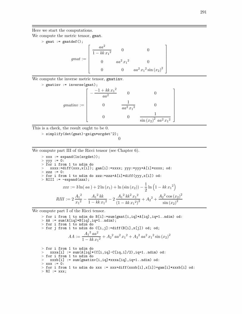
291
Here we start the computations.We compute the metric tensor, gmat.
> gmat := gmatdef();
gmat :=
aa2
1 − kk x12
0 0
0 aa2 x12 0
0 0 aa2 x12 sin (x2)
2
We compute the inverse metric tensor, gmatinv.> gmatinv := inverse(gmat);
gmatinv :=
− −1 + kk x12
aa20 0
01
aa2 x12
0
0 01
sin (x2)2 aa2 x1
2
This is a check, the result ought to be 0.> simplify(det(gmat)-gsign*srgdet^2);
0
We compute part III of the Ricci tensor (see Chapter 6).
> xxx := expand(ln(srgdet));> yyy := 0:> for i from 1 to ndim do> xxxx:=diff(xxx,x[i]); gam[i]:=xxxx; yyy:=yyy+A[i]*xxxx; od:> zzz := 0:> for i from 1 to ndim do zzz:=zzz+A[i]*diff(yyy,x[i]) od:> RIII := -expand(zzz);
xxx := 3 ln( aa ) + 2 ln (x1) + ln (sin (x2)) −1
2ln(1 − kk x1
2)
RIII := 2A1
2
x12− A1
2 kk
1 − kk x12− 2
A12 kk2 x1
2
(1 − kk x12)2
+A22 +
A22 cos (x2)
2
sin (x2)2
We compute part I of the Ricci tensor.> for i from 1 to ndim do B[i]:=sum(gmat[i,iq]*A[iq],iq=1..ndim) od:> AA := sum(A[iq]*B[iq],iq=1..ndim);> for i from 1 to ndim do> for j from 1 to ndim do C[i,j]:=diff(B[i],x[j]) od; od;
AA :=A1
2 aa2
1 − kk x12
+A22 aa2 x1
2 +A32 aa2 x1
2 sin (x2)2
> for i from 1 to ndim do> xxxa[i] := sum(A[iq]*(C[i,iq]-C[iq,i]/2),iq=1..ndim) od:> for i from 1 to ndim do> xxxb[i] := sum(gmatinv[i,iq]*xxxa[iq],iq=1..ndim) od:> xxx := 0:> for i from 1 to ndim do xxx := xxx+diff(xxxb[i],x[i])+gam[i]*xxxb[i] od:> RI := xxx;
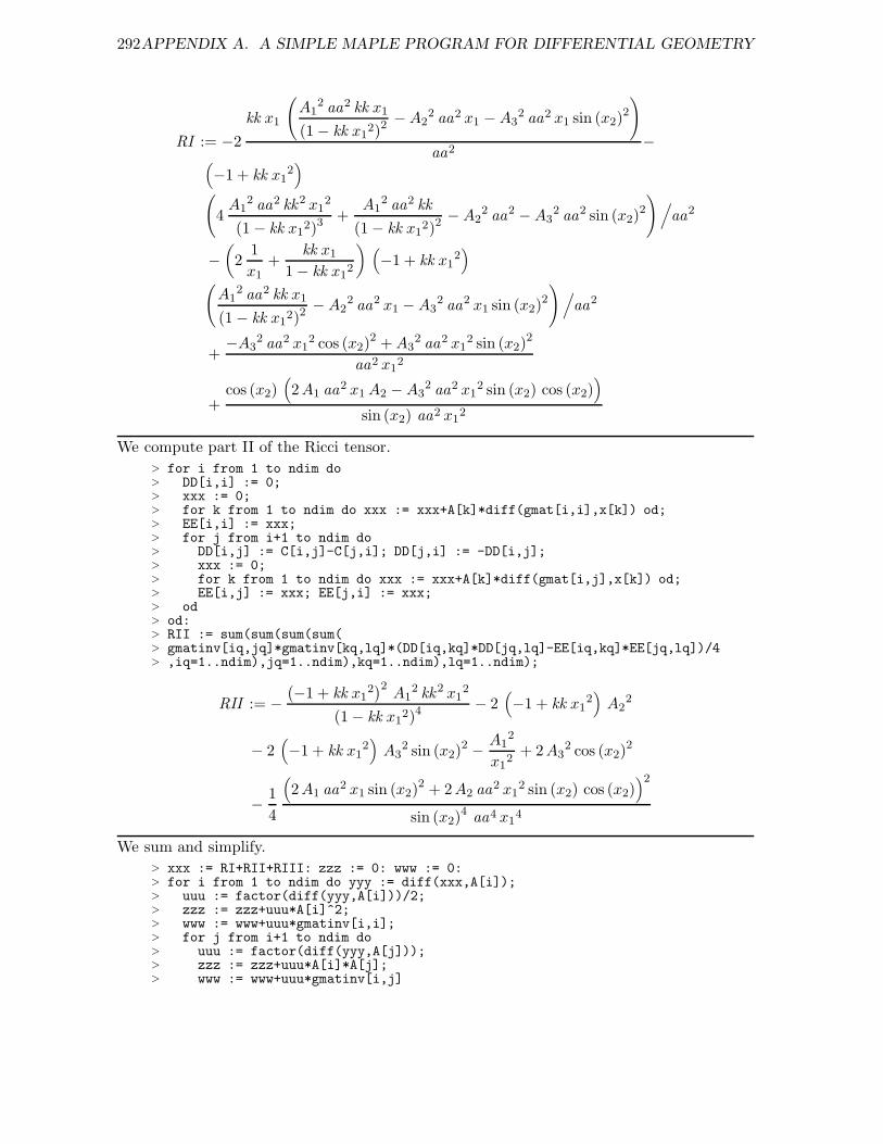
292APPENDIX A. A SIMPLE MAPLE PROGRAM FOR DIFFERENTIAL GEOMETRY
RI := −2
kk x1
(A1
2 aa2 kk x1
(1 − kk x12)2
−A22 aa2 x1 −A3
2 aa2 x1 sin (x2)2
)
aa2−
(−1 + kk x1
2)
(4A1
2 aa2 kk2 x12
(1 − kk x12)3
+A1
2 aa2 kk
(1 − kk x12)2
−A22 aa2 −A3
2 aa2 sin (x2)2
)/aa2
−(
21
x1+
kk x1
1 − kk x12
) (−1 + kk x1
2)
(A1
2 aa2 kk x1
(1 − kk x12)2
−A22 aa2 x1 −A3
2 aa2 x1 sin (x2)2
)/aa2
+−A3
2 aa2 x12 cos (x2)
2 +A32 aa2 x1
2 sin (x2)2
aa2 x12
+cos (x2)
(2A1 aa2 x1A2 −A3
2 aa2 x12 sin (x2) cos (x2)
)
sin (x2) aa2 x12
We compute part II of the Ricci tensor.> for i from 1 to ndim do> DD[i,i] := 0;> xxx := 0;> for k from 1 to ndim do xxx := xxx+A[k]*diff(gmat[i,i],x[k]) od;> EE[i,i] := xxx;> for j from i+1 to ndim do> DD[i,j] := C[i,j]-C[j,i]; DD[j,i] := -DD[i,j];> xxx := 0;> for k from 1 to ndim do xxx := xxx+A[k]*diff(gmat[i,j],x[k]) od;> EE[i,j] := xxx; EE[j,i] := xxx;> od> od:> RII := sum(sum(sum(sum(> gmatinv[iq,jq]*gmatinv[kq,lq]*(DD[iq,kq]*DD[jq,lq]-EE[iq,kq]*EE[jq,lq])/4> ,iq=1..ndim),jq=1..ndim),kq=1..ndim),lq=1..ndim);
RII := −(−1 + kk x1
2)2A1
2 kk2 x12
(1 − kk x12)4
− 2(−1 + kk x1
2)A2
2
− 2(−1 + kk x1
2)A3
2 sin (x2)2 − A1
2
x12
+ 2A32 cos (x2)
2
− 1
4
(2A1 aa2 x1 sin (x2)
2 + 2A2 aa2 x12 sin (x2) cos (x2)
)2
sin (x2)4 aa4 x1
4
We sum and simplify.> xxx := RI+RII+RIII: zzz := 0: www := 0:> for i from 1 to ndim do yyy := diff(xxx,A[i]);> uuu := factor(diff(yyy,A[i]))/2;> zzz := zzz+uuu*A[i]^2;> www := www+uuu*gmatinv[i,i];> for j from i+1 to ndim do> uuu := factor(diff(yyy,A[j]));> zzz := zzz+uuu*A[i]*A[j];> www := www+uuu*gmatinv[i,j]
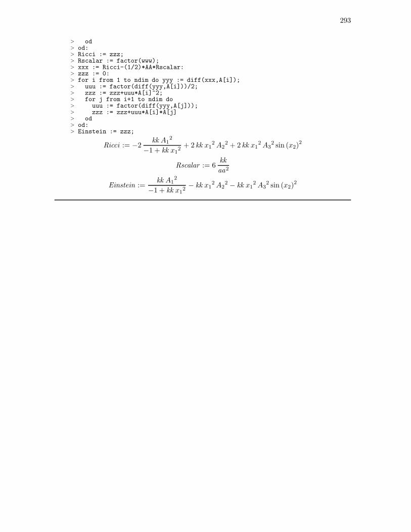
293
> od> od:> Ricci := zzz;> Rscalar := factor(www);> xxx := Ricci-(1/2)*AA*Rscalar:> zzz := 0:> for i from 1 to ndim do yyy := diff(xxx,A[i]);> uuu := factor(diff(yyy,A[i]))/2;> zzz := zzz+uuu*A[i]^2;> for j from i+1 to ndim do> uuu := factor(diff(yyy,A[j]));> zzz := zzz+uuu*A[i]*A[j]> od> od:> Einstein := zzz;
Ricci := −2kk A1
2
−1 + kk x12
+ 2 kk x12A2
2 + 2 kk x12A3
2 sin (x2)2
Rscalar := 6kk
aa2
Einstein :=kk A1
2
−1 + kk x12− kk x1
2A22 − kk x1
2A32 sin (x2)
2
294APPENDIX A. A SIMPLE MAPLE PROGRAM FOR DIFFERENTIAL GEOMETRY
Appendix B
Group theory
This appendix gives a very brief summary of some central concepts of group theory, which isthe mathematical theory of symmetry transformations.
B.1 The group axioms
A group in the mathematical sense is a set G of group elements, with a mathematical operationof group multiplication which assigns to any two group elements f and g a third element fg.The number of elements in G is denoted by |G|, it is the order of the group.
Three simple axioms define what it means to call G a group:
(i) G contains a unit element e such that eg = g for all g ∈ G.
(ii) Every g ∈ G has an inverse, g−1, such that g−1g = e.
(iii) The group multiplication is associative: f(gh) = (fg)h for all f, g, h ∈ G.
If in addition the group multiplication is commutative, that is, if fg = gf for all f, g ∈ G,then we have a commutative group, also called an Abelian group. The non-Abelian groupsare usually the most interesting cases.
That the group multiplication is associative, means that it is unnecessary to write paren-theses in a product of more than two factors. In particular, powers are uniquely defined:g2 = gg, g3 = gg2 = g2g, g4 = gg3 = g2g2 = g3g, and so on.
It follows from the axioms that e2 = e. The equation g2 = g has g = e as its only solution,because it implies that
g = eg = (g−1g)g = g−1g2 = g−1g = e . (B.1)
Thus, a group can not contain more than one unit element. It follows that gg−1 = e, since
(gg−1)2 = (gg−1)(gg−1) = g((g−1g)g−1) = g(eg−1) = gg−1 . (B.2)
Furthermore,
ge = g(g−1g) = (gg−1)g = eg = g . (B.3)
The inverse of any g ∈ G is unique, because if fg = e, then
f = fe = f(gg−1) = (fg)g−1 = eg−1 = g−1 . (B.4)
Since the inverse is unique, and gg−1 = e, it follows that (g−1)−1 = g. It also follows that(fg)−1 = g−1f−1, since g−1f−1fg = g−1eg = e.
295
296 APPENDIX B. GROUP THEORY
Transformation groups
G is a transformation group if the group elements of G are transformations over some setX, and if the group multiplication is composition of functions. To be more precise, any twoelements f, g ∈ G are functions, f : X → X and g : X → X, and the product h = fg is thefunction h : X → X defined such that h(x) = f(g(x)) for all x ∈ X.
The unit element of a transformation group is the identity transformation, often denotedby I,
e(x) = I(x) = x for all x ∈ X . (B.5)
Every function f ∈ G has to be invertible, that is, for every y ∈ X the equation f(x) = ymust have a unique solution for x ∈ X. Then the inverse function f−1 is defined such that
f−1(y) = x when f(x) = y . (B.6)
The usefulness of the group axioms is due especially to the fact that functional compositionis automatically associative: given any three functions h : X → Y , g : Y → Z and f : X → U ,the two composite functions a = f(gh) : X → U and b = (fg)h : X → U are identical becausethey are defined in the same way,
a(x) = b(x) = f(g(h(x))) for all x ∈ X . (B.7)
Every group may be regarded as a transformation group. In fact, a group G is a trans-formation group acting on itself by group multiplication: let f ∈ G transform g ∈ G intofg. The transformation g 7→ fg may be called a left translation. The group product f1f2
corresponds to the transformation g 7→ f1f2g, which we obtain by transforming first by f2
and afterwards by f1, that is, g 7→ f2g 7→ f1f2g.An alternative is to let f ∈ G act on G by the right translation g 7→ gf−1. Here we
need to use f−1 instead of f , in order that g 7→ g(f1f2)−1 becomes the composite function
g 7→ gf2−1 7→ gf2
−1f1−1.
Subgroups
A subset H ⊂ G is a subgroup of G if it is a group with the same group multiplication as inG. Two trivial exemples are e, which is a subgroup of order one, and G itself, which wedefine to be a subgroup.
A less trivial example is
H = gn | n = 0,±1,±2, . . . , (B.8)
for an arbitrary element g ∈ G. We define g0 = e, and g−n = (g−1)n for n > 0, and we mayshow in general that gm gn = gn gm = gm+n. H is then what we call a cyclic subgroup ofG, generated by g. We say that g is a cyclic element of G, and that G is cyclic, if the cyclicsubgroup generated by g, is all of G. A cyclic group is Abelian.
A subgroup H is by definition closed under multiplication: fg ∈ H whenever f ∈ H andg ∈ H. Furthermore, the unit element of H has to be the same as in G, because it is a solutionof the equation g2 = g, and g = e is the only solution in G. Since inverses are unique, it alsofollows that H has to be closed under inversion: g−1 ∈ H for every g ∈ H.
Conversely, it is easy to prove that a subset H ⊂ G is a subgroup if it is closed undermultiplication and inversion. Thus, this double condition is both necessary and sufficient.Note that if H is finite, closure under multiplication implies closure under inversion.

B.1. THE GROUP AXIOMS 297
Cosets
Given a subgroup H ⊂ G and an element g ∈ G. We define a left coset of H as
gH = gh | h ∈ H , (B.9)
and a right coset of H as
Hg = hg | h ∈ H . (B.10)
The set of all left cosets we call G/H, and the set of all right cosets we call H\G.H itself is a coset, both left and right, since H = gH = Hg for all g ∈ H. Since e ∈ H,
and g = ge = eg, we always have g ∈ gH and g ∈ Hg. In particular, g ∈ H if either gH = Hor Hg = H.
We have that gH = fH if f ∈ gH, and Hg = Hf if f ∈ Hg. Hence, two left cosets gHand hH are identical, gH = hH = fH, if they have at least one common element f , and thesame is true for two right cosets Hg and Hh.
It follows that a subgroup H ⊂ G splits G into disjoint left cosets, and into disjoint rightcosets. The number of elements in every coset equals |H|, the order of H. If G is of finiteorder, this means that the order of H must be a factor of the order of G, that is, the ratio|G|/|H| must be an integer.
This result is very interesting if for example |G| is a prime number p. In that case therecan exist no subgroup of G apart from the trivial subgroup e, of order one, and the wholegroup G, of order p. The cyclic subgroup generated by any element g 6= e must be all of G.
A group of prime order must be cyclic, and every element g 6= e must be cyclic.
Homogeneous spaces
Let G be a group with H as a subgroup, and let X = G/H. Then G acts as a transformationgroup over X, such that every f ∈ G transforms a coset x = gH into f(x) = fgH. X is ahomogeneous space for the group G, that is, G acts transitively on X, which means that fortwo arbitrary cosets x = gH and y = hH there always exists an element f ∈ G such thaty = f(x). The proof is simple: choose f = hg−1, then fg = h and fgH = hH.
H is the fixed point group of the single point x0 = H ∈ X, that is,
H = g ∈ G | g(x0) = x0 . (B.11)
Every homogeneous space of a transformation group G may be identified with the quotientset G/H, where H is the fixed point group of an arbitrary point in X. Hence |X|, the numberof points in a homogeneous space X, must be a divisor of |G|, the order of G, when G is finite.
Conjugation classes
If f, g ∈ G then h = fgf−1 is the conjugate of g by f . Conjugation preserves the groupmultiplication,
(fg1f−1)(fg2f
−1) = f(g1g2)f−1 . (B.12)
If f = e then g = fgf−1. In general, g = fgf−1 if and only if f and g commute, gf = fg.Hence, conjugation is a trivial operation in an Abelian group.
298 APPENDIX B. GROUP THEORY
Every element g ∈ G belongs to a conjugation class
C(g) = fgf−1 | f ∈ G . (B.13)
Two conjugation classes in G are either identical, or they have no elements in common.A conjugation class in G is a homogeneous space for G, hence its number of elements must
be a divisor of |G|, when G is finite.
Invariant subgroups
In an Abelian group G there is no difference between left and right cosets: gH = Hg forevery subgroup H and every element g ∈ G. Also in a non-Abelian group G it is possiblefor a subgroup H to have the property that gH = Hg for all g ∈ G. In general we say thata subgroup H ⊂ G is invariant, or normal, if the left cosets of H are identical to the rightcosets.
That gH = Hg means that for every h1 ∈ H there is an h2 ∈ H such that gh1 = h2g,that is, h2 = gh1g
−1. Thus, an invariant subgroup of G is invariant under conjugation by anarbitrary element g ∈ G.
We may multiply subsets A,B ⊂ G by defining
AB = ab | a ∈ A, b ∈ B . (B.14)
We have for example that HH = H for every subgroup H ⊂ G.This multiplication turns G/H into a group, which we may call a quotient group, whenever
H is an invariant subgroup. The essential point is that the product of two cosets gH = Hgand hH = Hh is a coset when H is invariant:
(gH)(hH) = g(Hh)H = g(hH)H = (gh)(HH) = (gh)H . (B.15)
Homomorphism and isomorphism
Let G and H be two groups. A function ρ : G→ H preserving the group multiplication, suchthat ρ(fg) = ρ(f) ρ(g) for all f, g ∈ G, is called a homomorphism. The image of ρ,
ρ(G) = ρ(g) | g ∈ G , (B.16)
is then a subgroup of H, while the kernel of ρ,
K = ρ−1(eH) = g ∈ G | ρ(g) = eH , (B.17)
is a subgroup of G. We write eG and eH in order to distinguish the unit elements of G andH. It is necessary that ρ(eG) = eH , because (ρ(eG))2 = ρ(eG).
The homomorphism ρ : G → H is an isomorphism if ρ(G) = H and ρ−1(eH) = eG. Inthis case ρ is an invertible function, and the function ρ−1 : H → G is also an isomorphism.Two groups G and H are isomorphic when there exists an isomorphism between them. In asense two isomorphic groups G and H are the same group: the two multiplication tables areidentical, except that the group elements have different names.
An automorphism of a group G is an isomorphism of the group with itself. Conjugationby an element f ∈ G, that is, the function ρ : g 7→ fgf−1, is an example of an automorphism.
B.2. EXAMPLES 299
This special type of automorphism is called an inner automorphism, and all the rest are thenouter automorphisms.
All the automorphisms of a group G form a group, this is the symmetry group of thegroup G. The inner automorphisms form an invariant subgroup of the automorphism group.
The kernel K of a homomorphism ρ : G→ H is not only a subgroup of G, it is an invariantsubgroup. Hence G/K is a group. The homomorphism ρ from G to H is an isomorphismbetween ρ(G) and the quotient group G/K.
B.2 Examples
The symmetric group
Given two sets X and Y . That a function f : X → Y is invertible means that there exists aninverse function f−1 : Y → X such that f−1(f(x)) = x for all x ∈ X and f(f−1(y)) = y forall y ∈ Y .
A permutation of the elements in a set X is an invertible function f : X → X. All thepermutations over X together form a group, the symmetric group SX . Every transformationgroup over X is a subgroup of SX . In particular, every group G is (isomorphic to) a subgroupof SG.
SX and SY are isomorphic groups if there exists an invertible function f : X → Y . Thento every permutation g ∈ SX corresponds a permutation fgf−1 ∈ SY , and the mappingg 7→ fgf−1 is an isomorphism.
Matrix groups. The General Linear group
Matrix multiplication is associative, and many of the groups we meet in physics are matrixgroups, consisting of n × n matrices for some n = 1, 2, 3, . . .. The matrix elements may bereal or complex. The identity matrix
I =
1 0 . . . 00 1 . . . 0...
.... . .
...0 0 . . . 1
(B.18)
is the unit element of a matrix group, IA = AI for all n× n matrices A.Every matrix A in a matrix group has to be invertible, that is, the inverse matrix A−1 has
to exist, or equivalently, we must have (detA) 6= 0. Every matrix group of real or complexn×n matrices is a subgroup of the General Linear group GL(n,C), consisting of all complexn× n matrices with nonzero determinant.
A subgroup of GL(n,C) is for example GL(n,R), consisting of all invertible real n × nmatrices. Two other subgroups are the Special Linear groups SL(n,C) and SL(n,R), con-sisting of all complex, or real, n × n matrices having determinant equal to 1. SL(n,R) is asubgroup of GL(n,R) as well as of SL(n,C).
The Orthogonal group
Yet other subgroups of GL(n,C) are the Orthogonal groups O(n,C) and O(n) = O(n,R),consisting of all orthogonal n× n matrices, complex or real. A matrix A is orthogonal when
300 APPENDIX B. GROUP THEORY
it is invertible and
AT = A−1 . (B.19)
AT is the transpose of A (a transposition is a reflection about the matrix diagonal). When A isa finite dimensional matrix we may take the determinant of the above equation and obtain theequation detA = (detA)−1, which has the two solutions detA = ±1. The Special Orthogonalgroups SO(n,C) and SO(n) = SO(n,R) are subgroups of O(n,C) and O(n) = O(n,R)consisting of those matrices having determinant +1.
The condition AT = A−1, or ATA = I, may be generalized to
ATGA = G , (B.20)
whereG is an invertible matrix, a metric. With G = I this defines again the orthogonal groupsO(n,C) and O(n,R). If G is diagonal and has m times +1 and n−m times −1 on its diagonal,this defines the pseudo-orthogonal groups O(m,n−m,C) and O(m,n−m) = O(m,n−m,R).Note that the groups O(m,n−m,C) and O(n−m,m,C) are isomorphic (why?). A subgroupof O(m,n−m) is again SO(m,n−m), for example.
The group O(3), as an example, consists of all rotations and reflections in our familiarthree dimensional space, whereas SO(3) consists of the rotations alone, without the reflections.O(1, 3) is the group of all Lorentz transformations, including the reflections P , T and PT ,whereas SO(1, 3) includes the space and time inversion PT , but not the space inversion P orthe time reversion T .
The Symplectic group
The condition ATGA = G defines the Symplectic groups Sp(2n,C) and Sp(2n,R) if G is anantisymmetric and invertible (2n) × (2n) matrix, for example,
G =
(0 −II 0
), (B.21)
where we take the zero matrix 0 and the identity matrix I to be n× n matrices.
The Unitary group
The Unitary group U(n) consists of all unitary n×n matrices. A complex matrix A is unitaryif
A† = A−1 . (B.22)
Here A† is the Hermitean conjugate of A, that is, the transposed and complex conjugated ma-trix. With finite dimensional matrices we may take the determinant of the equation A† = A−1
and obtain the equation (detA)∗ = (detA)−1, with the solution |detA| = 1, or equivalentlydetA = eiα with α real. The Special Unitary group U(n) consists of those unitary matri-ces having determinant +1. The unitary groups U(n) and SU(n) may be generalized toU(m,n −m) and SU(m,n −m), in a similar way as with the orthogonal groups.
B.3. LIE GROUPS 301
B.3 Lie groups
All matrix groups mentioned above are examples of Lie groups. A Lie group is a group inwhich the group elements depend on one or more continuous parameters, in such a way thatthe group operations, multiplication and inversion, are continuous and differentiable.
It is natural here to confine our discussion to the connected Lie groups. In a Lie groupG we may start with the unit element e and vary all parameters continuously. In that waywe may reach all elements of G, if G is connected. Otherwise, we generate a subset G0 ⊂ G,and G0 is a connected Lie group, which is an invariant subgroup of G. How to extend thesubgroup G0 so as to obtain the whole group G is then a problem in general group theorywhich is not of special interest in the theory of Lie groups.
The fundamental result in the theory of Lie groups may be formulated as follows:
The group multiplication in a connected Lie group is (in essence) uniquely deter-mined by the group multiplication in an arbitrarily small neighbourhood of the unitelement, and this again is determined by the Lie algebra of the group.
We will now see, in rough outline, how this result comes about, what a Lie algebra is, andwhat the connection is between the Lie group and its Lie algebra.
To be slightly more specific let us consider a connected Lie group G where the groupelements are real matrices of a given dimension n× n, and where the group multiplication ismatrix multiplication. This is anyway no serious restriction, since essentially all Lie groupsmay be represented as matrix groups (some Lie groups can not be faithfully represented asgroups of finite dimensional matrices). The unit element of G is the identity matrix I. Theinverse matrix A−1 has to exist for every A ∈ G, thus we must have (detA) 6= 0.
One parameter groups
Looking at small neighbourhoods about the identity I means in the limit looking at infinites-imal neighbourhoods. A group element infinitesimally close to I is of the form
A(α) = I + αX , (B.23)
where X is a finite matrix and α is an infinitesimal parameter. Then X is what we call agenerator, or infinitesimal generator, of the matrix group. By multiplying together infinitelymany matrices infinitesimally close to I we may generate the whole group.
We may formulate this somewhat vague idea more precisely by means of the exponentialfunction, which may be defined by either one of the two expressions
eX = limk→∞
(I +
X
k
)k
= I +X +X2
2+ · · · + Xk
k!+ · · · . (B.24)
What happens in the limit k → ∞ is, loosely speaking, that X/k becomes infinitesimal, andwe get a product of infinitely many factors all infinitesimally different from I. The infiniteseries is always convergent, for any matrix X. The exponential function of matrices is a directgeneralization of the exponential function of numbers (a number is just a 1 × 1 matrix).
Thus, the generalization of Equation (B.23), where α is infinitesimal, is
A(α) = eαX , (B.25)

302 APPENDIX B. GROUP THEORY
where α takes finite values. In this case the usual rule for the exponential function holds, that
A(α)A(β) = A(α + β) . (B.26)
Note that A(0) = I, and that (A(α))−1 = A(−α), because A(−α)A(α) = I. This means thatthe elements A(α) ∈ G form a subgroup of G. Every generator X of the Lie group definesin this way its own one parameter subgroup. Such one parameter subgroups in a Lie groupcorrespond to cyclic subgroups in a finite group.
As usual, the logarithm is the inverse of the exponential function,
elnX = ln(eX)
= X . (B.27)
Its series expansion is the usual one,
ln(I +X) = X − X2
2+X3
3− · · · + (−1)k+1 X
k
k+ · · · . (B.28)
However, this series converges only when the matrix X is “small”. More precisely, it convergesif all the eigenvalues of X have absolute values smaller than 1, and it diverges otherwise.
It follows from the definition of the exponential function that
det(eX)
= limk→∞
(det
(I +
X
k
))k
= limk→∞
(1 +
TrX
k
)k
= eTr X . (B.29)
TrX is the sum of the diagonal elements of the matrix X. We use the following relation,
det(I + ǫX) =
∣∣∣∣∣∣∣∣∣∣
1 + ǫX11 ǫX12 . . . ǫX1n
ǫX21 1 + ǫX22 . . . ǫX2n...
.... . .
...ǫXn1 ǫXn2 . . . 1 + ǫXnn
∣∣∣∣∣∣∣∣∣∣
= 1 + ǫTrX + (terms of order ǫ2) . (B.30)
The Campbell–Baker–Hausdorff theorem
The commutator between two matrices X and Y is defined as
[X,Y ] = XY − Y X . (B.31)
The usual rule that eX eY = eX+Y holds without restrictions if X and Y commute, thatis, if [X,Y ] = 0. The generalization to the case [X,Y ] 6= 0 is the so called Campbell–Baker–Hausdorff theorem, that eX eY = eZ , where
Z = X + Y +1
2[X,Y ] + (commutators of commutators) . (B.32)
The theorem does not hold for completely arbitrary exponents X and Y , because it mayhappen that the series for Z is infinite and divergent, but it always holds when X and Yare “sufficiently small”. An important assumption in the proof, even though the formula issomewhat more generally valid, is that all the eigenvalues of the matrix
U = eX eY − I (B.33)
B.3. LIE GROUPS 303
should be smaller than 1, so that we may use the series expansion to compute Z = ln(I +U).This calculation is straightforward in principle, but it is not very easy to prove the Campbell–Baker–Hausdorff theorem in such a way, by brute force. Try it!
Here is an alternative proof, using the formula
eβX Y e−βX = Y + β [X,Y ] +β2
2[X, [X,Y ]] + · · · + βk
k![X, [X, . . . [X,Y ] . . .]] + · · · . (B.34)
This formula is trivial for β = 0, and it holds in general because it solves the following firstorder differential equation for V (β) = eβX Y e−βX ,
dV
dβ=
d(eβX)
dβY e−βX + eβX Y
d(e−βX)
dβ= XV − V X = [X,V ] . (B.35)
Given the matrices X and Y , let us define W (α) such that W (0) = Y and eW (α) = eαX eY .Differentiation of this equation and multiplication from the right by e−W = e−Y e−αX givesthat
d(eW )
dαe−W = X . (B.36)
It is tempting to set the left hand side of this equation simply equal to W ′ = dW/dα,but that is correct only under the assumption that W and W ′ commute. To find the correctformula in general we have to go back to the definition of the exponential function. We havethat
d(eW )
dα= lim
n→∞
n∑
k=1
(I +
W
n
)k−1 W ′
n
(I +
W
n
)n−k
=
∫ 1
0dβ eβW W ′ e(1−β)W , (B.37)
and hence,
X =d(eW )
dαe−W =
∫ 1
0dβ eβW W ′ e−βW (B.38)
= W ′ +1
2[W,W ′] + · · · + 1
(k + 1)![W, [W, . . . [W,W ′] . . .]] + · · · .
We need the inverse formula,
W ′ = X − 1
2[W,X] +
1
12[W, [W,X]] + · · · + Bk
k![W, [W, . . . [W,X] . . .]] + · · · , (B.39)
where Bk is the k-th Bernoulli number,
B0 = 1 , B1 = −1
2, B2 =
1
6, B4 = − 1
30, B6 =
1
42,
B3 = B5 = . . . = B2j+1 = . . . = 0 . (B.40)
Observe that the coefficients of the series in Equation (B.38) are the same as in the powerseries
ex − 1
x= 1 +
1
2x+
1
6x2 + · · · + 1
(k + 1)!xk + · · · . (B.41)
304 APPENDIX B. GROUP THEORY
We may then prove Equation (B.39) rather directly using Equation (B.38), together with thedefinition of the Bernoulli numbers,
x
ex − 1=
∞∑
k=0
Bk
k!xk . (B.42)
Equation (B.39) is a non-linear differential equation forW (α). The initial valueW (0) = Y ,together with the form of the equation, with commutators, implies the Campbell–Baker–Hausdorff theorem, which we wanted to prove.
In order to see this in a little more detail, we may calculate the third order terms in theCampbell–Baker–Hausdorff formula for Z = W (1), saying that X and Y are of first orderand [X,Y ] of second order. Differentiation of Equation (B.39) gives that
W ′′ = −1
2[W ′,X] +
1
12[W ′, [W,X]] +
1
12[W, [W ′,X]] + · · · . (B.43)
Inserting α = 0 and calculating to third order we get that
W ′(0) = X − 1
2[Y,X] +
1
12[Y, [Y,X]] + · · · , (B.44)
W ′′(0) =1
4[[Y,X],X] +
1
12[X, [Y,X]] + · · · =
1
6[X, [X,Y ]] + · · · .
Hence we have, to third order,
Z = W (0) +W ′(0) +1
2W ′′(0) + · · · (B.45)
= X + Y +1
2[X,Y ] +
1
12[X, [X,Y ]] +
1
12[Y, [Y,X]] + · · · .
B.4 Lie algebras
The infinitesimal generators of a Lie group form a real vector space, this means that an arbi-trary linear combination αX+βY of two generators X and Y , with arbitrary real coefficientsα and β, is a generator. To prove this we consider A = eǫαX eǫβY , where ǫ is a real number.Being a product of two group elements, A itself is a groupelement, and in the limit when ǫ isinfinitesimal, we have that
A = I + ǫ (αX + βY ) . (B.46)
The commutator [X,Y ] is also a generator. To prove this we consider
A = eδX eδY e−δX e−δY , (B.47)
which is product of four group elements, and therefore a group element itself. In the limitwhen ǫ = δ2 is infinitesimal it follows from the Campbell–Baker–Hausdorff theorem that
A = I + ǫ [X,Y ] . (B.48)
The vector space of infinitesimal generators, with the commutator product, is the Liealgebra of the group. The essential contents of the Campbell–Baker–Hausdorff theorem is
B.5. EXAMPLES 305
that the group multiplication in a small, but finite, region around the unit element of a Liegroup is completely determined by the Lie algebra.
Note that the fundamental algebraic structure of a Lie algebra is the commutator product[X,Y ]. The properties characterising the commutator product in a Lie algebra are bilinearity:
[X,αY + βZ] = α[X,Y ] + β[X,Z] ,
[αX + βY,Z] = α[X,Y ] + β[Y,Z] , (B.49)
antisymmetry:
[X,Y ] = −[Y,X] , (B.50)
and the Jacobi identity:
[X, [Y,Z]] + [Y, [Z,X]] + [Z, [X,Y ]] = 0 . (B.51)
All of these properties follow directly from the definition [X,Y ] = XY −Y X. For example,the Jacobi identity follows because the usual matrix product XY is associative, so that
[X, [Y,Z]] = XY Z −XZY − Y ZX + ZY X . (B.52)
However, it is quite possible to forget about the definition [X,Y ] = XY −Y X and take insteadthe three basic properties of the commutator product, the bilinearity, the antisymmetry andthe Jacobi identity, as axioms defining a Lie algebra. We may very well have an abstractLie algebra, with a commutator product [X,Y ], where the elements X and Y are no longermatrices, and where the associative product XY is not even defined.
B.5 Examples
The Lie algebras of the general linear groups GL(n,R) and GL(n,C) are usually calledgl(n,R) and gl(n,C).
One basis for gl(n,R) consists of the n2 matrices Ejk, for j, k = 1, 2, . . . , n, with matrix
elements
(Ejk)rs = δj
rδks . (B.53)
Multiplication of two such basis matrices gives either 0 or a third basis matrix,
Ejk E
lm = δl
k Ejm . (B.54)
This gives the following commutation relations, defining the Lie algebra gl(n,R),
[Ejk, E
lm] = δl
k Ejm − δj
mElk . (B.55)
The Lie algebra gl(n,C) is twice as large as gl(n,R), since it also contains basis matrices
F jk = iEj
k . (B.56)
We then get the following new commutation relations,
[Ejk, F
lm] = δl
k Fjm − δj
m F lk ,
[F jk , F
lm] = −δl
k Ejm + δj
mElk . (B.57)
306 APPENDIX B. GROUP THEORY
Appendix C
Statistical mechanics
Here we summarize briefly some of the statistical mechanics used in cosmology.Given a physical system consisting of different types of particles, with Ni particles of type
i. Let a = 1, 2, . . . enumerate the quantum mechanical states of the system, with variablenumbers of particles of each type. In state number a the energy is Ea, and the number ofparticles of type i is Nia.
The particles are identified by certain additive quantum numbers Q1, Q2, . . ., which wechoose to call “charges”, for example the electric charge q, baryon number B and leptonnumber L. We assume that all these charges are conserved. A particle of type i has thevalues Q1i, Q2i, . . . of the charges, and the total charge QJ in the state a is
QJa =∑
i
NiaQJi . (C.1)
We imagine an ensemble of N such systems, which may exchange both energy and parti-cles, in such a way that the average energy E is fixed, and also the avarage values Q1, Q2, . . .of the various conserved charges. Assume that Na of the N systems are in the state a. Thus,we have that
∑
a
Na = N ,
∑
a
NaEa = NE , (C.2)
∑
a
NaQJa = NQJ , (J = 1, 2, . . .) .
The probability of this distribution of the systems in the ensemble is proportional to themultinomial coefficient
W =N !∏a Na!
. (C.3)
We assume that N is such a large number that the numbers Na separately are large, andhence that we may use the following approximation,
lnW = N lnN −N −∑
a
(Na lnNa −Na) = −∑
a
Na(lnNa − lnN ) . (C.4)
307

308 APPENDIX C. STATISTICAL MECHANICS
The last equality follows because∑
a Na = N . We may introduce the dimensionless entropy,defined as
S =lnWN = −
∑
a
Pa lnPa , (C.5)
where Pa = Na/N is the probability of finding a system in the state a if it is picked at randomfrom the ensemble.
We find the most probable distribution by maximizing W, or equivalently the entropy S,under the constraints given in Equation (C.2). We introduce Lagrange multipliers α, β, andγJ , and solve the equations
∂
∂Pa
(S − α
(∑
a
Pa − 1
)− β
(∑
a
PaEa − E
)
−∑
J
γJ
(∑
a
PaQJa −QJ
))= 0 . (C.6)
The solution is Pa = Pa, with the definition
Pa = e−1−α−βEa−∑
JγJQJ . (C.7)
Pa is the probability of finding a system in the state a if it is picked at random from anensemble in equilibrium. The Lagrange multiplier α is chosen so that
∑a Pa = 1. We define
the grand canonical partition function as
Ξ = e1+α =∑
a
e−βEa−∑
JγJQJ . (C.8)
The Lagrange multiplier β is the inverse of the absolute temperature T ,
β =1
kBT, (C.9)
where kB is Boltzmann’s constant. We may define the chemical potential µJ for the chargeQJ by the relation βµJ = −γJ , and we define the chemical potential for particles of type i as
µi =∑
J
µJQJi . (C.10)
Then we may write
Pa = e−1−α−β(Ea−∑
iµiNia) . (C.11)
Equation (C.10) has interesting consequences. First, we know that every particle type hasits own antiparticle with the opposite sign of all charge quantum numbers, and the equationtells us that the chemical potential is of equal magnitude but opposite sign for particle andantiparticle. In particular, the chemical potential must be zero for neutral particles, that is,particles having all charges equal to zero and hence being their own antiparticles. The photonis the most important example of a neutral particle. The neutrino is not a neutral particle,even though it is electrically neutral, because it has lepton number 1.
309
Second, since all the charge quantum numbers are conserved, the equation tells us thatin equilibrium the chemical potential is conserved in all particle reactions (remember thatthe chemical potentials characterize an equilibrium state, and are undefined outside of equi-librium). For example, an electron (e−) and a proton (p) may be converted to an electronneutrino (νe) and a neutron (n), and vice versa, according to the reaction equation
e− + p ↔ νe + n . (C.12)
The equilibrium condition for these two opposite processes is that the chemical potentialssatisfy the relation
µe− + µp = µνe + µn . (C.13)
All termodynamical quantities may be computed from the partition function
Ξ = Ξ(β, µ1, µ2, . . .) = e1+α =∑
a
e−β(Ea−∑
iµiNia) . (C.14)
For example the average particle numbers and the average energy of one system,
〈Ni〉 =∑
a
PaNia =1
β
∂
∂µiln Ξ ,
〈E〉 =∑
a
PaEa = − ∂
∂βln Ξ +
∑
i
µi〈Ni〉 . (C.15)
Ideal gas
In an ideal gas the interactions between particles can be neglected. A state a of such a systemis specified by all the occupation numbers Niα, where the first index i identifies a particletype, and the second index α identifies a one particle state for particles of type i. The oneparticle energies are Eiα. Thus, in the state a the number of particles of type i is
Nia =∑
α
Niα , (C.16)
and the energy is
Ea =∑
i
∑
α
NiαEiα . (C.17)
This means that each exponential function in Equation (C.14) factorizes into one particlefactors,
e−β(Ea−∑
iµiNia) =
∏
i
∏
α
e−βNiα(Eiα−µi) . (C.18)
The sum over states in Equation (C.14) is a multiple sum over occupation numbers Niα, onesum for each index pair iα, and the partition function Ξ factorizes into a product
Ξ =∏
i
∏
α
Ξiα , (C.19)
310 APPENDIX C. STATISTICAL MECHANICS
with
Ξiα =∑
n
e−βn(Eiα−µi) . (C.20)
Since the particles do not interact we may deal with the different particle types one at a time.In order to simplify the discussion we will assume from now on that there is only one type ofparticles, so that we may leave out the particle index i.
If the particles are fermions, then
Ξα = 1 + e−β(Eα−µ) , (C.21)
because the particle number n in the one particle state α can only be either 0 or 1. Forbosons, the number of particles in one and the same state is unlimited, so that
Ξα =1
1 − e−β(Eα−µ). (C.22)
This gives the logarithm of the partition function for an ideal gas of bosons or fermions as asum over one particle states,
ln Ξ = ∓∑
α
ln(1 ∓ e−β(Eα−µ)
). (C.23)
The signs are − for bosons and + for fermions. The average particle number and energy arethen given as
〈N〉 =∑
α
1
eβ(Eα−µ) ∓ 1,
〈E〉 =∑
α
Eα
eβ(Eα−µ) ∓ 1. (C.24)
In a large volume V the sum over α may be approximated by an integral over the threedimensional momentum p, such that
ln Ξ = ∓gVh3
∫d3p ln
(1 ∓ e−β(E(p)−µ)
). (C.25)
The degeneracy factor g is the number of inner degrees of freedom of a particle. The relativisticenergy of a particle of mass m and momentum p is
E = E(p) = c√m2c2 + |p|2 . (C.26)
This gives the following expressions for the particle number density and energy density,
n =〈N〉V =
g
h3
∫d3p
1
eβ(E(p)−µ) ∓ 1,
ρc2 =〈E〉V =
g
h3
∫d3p
E(p)
eβ(E(p)−µ) ∓ 1. (C.27)

311
The integrals may be computed exactly in the special case when both the mass and thechemical potential are zero. That m = 0 means that we have a relativistic gas, in which allthe particles move with the speed of light. Then we have, for an ideal gas of bosons, that
n = nb = gζ(3)(kBT )3
π2(hc)3, (C.28)
ρc2 = ρbc2 = g
π2(kBT )4
30(hc)3.
The constant ζ(3) = 1.202057 . . . is the Riemann zeta function of 3. For an ideal gas ofrelativistic fermions we have that
n = nf =3
4nb , (C.29)
ρc2 = ρfc2 =
7
8ρbc
2 .
The ratio between fermions and bosons is simply a factor of 3/4 in the number density anda different factor of 7/8 in the energy density, independent of the temperature T .
Thus, the energy density of a relativistic gas consisting of several types of particles maybe written as
ρc2 = g∗π2(kBT )4
30(hc)3,
where g∗ is the effective number of degrees of freedom,
g∗ =∑
b
gb +7
8
∑
f
gf . (C.30)
Here∑
b is a sum over all types of particles that are bosons, whereas∑
f is a sum over alltypes of fermions, with a factor 7/8 which is the ratio between the energy densities of fermionsand bosons. The energy density is proportional to g∗ and to T 4.
Setting m = 0 and µ = 0 will always be a good approximation when the temperatureis high, or more precisely when m << kBT and |µ| << kBT . This simple formula for theenergy density is therefore very interesting and useful, not least in cosmology.
Pressure
The general formula for pressure,
P =1
βV ln Ξ , (C.31)
gives for an ideal gas of bosons or fermions that
P = ∓ g
βh3
∫d3p ln
(1 ∓ e−β(E−µ)
)= ∓4πg
βh3
∫ ∞
0dp p2 ln
(1 ∓ e−β(E−µ)
). (C.32)
We may change the integration variable here from p = |p| to E = c√m2c2 + p2. Since
E2 = c2(m2c2 + p2) it follows that
E dE = c2p dp , (C.33)
312 APPENDIX C. STATISTICAL MECHANICS
and,
P = ∓ 4πg
βc2h3
∫ ∞
mc2dE pE ln
(1 ∓ e−β(E−µ)
). (C.34)
Equation (C.33) also gives that
pE = c2p2 dp
dE=c2
3
d(p3)
dE. (C.35)
By partial integration we find that
P =4πg
3h3
∫ ∞
mc2dE
p3
eβ(E−µ) ∓ 1. (C.36)
This integral may also be written as
P =4πgc2
h3
∫ ∞
0dp
p4
3E
1
eβ(E−µ) ∓ 1=
g
h3
∫d3p
p · v3
1
eβ(E−µ) ∓ 1, (C.37)
where v is the particle speed,
v =c2p
E=
cp√m2c2 + |p|2 . (C.38)
We see that in the case of a relativistic ideal gas, with m = 0 and p · v = pc = E, therelation P = ρc2/3 holds independent of the temperature and the chemical potential.
Index
active transformation, see transformation, ac-tive
coordinatetransformation, see transformation, of co-
ordinates
δ, see Kronecker δ, Dirac δ functionDirac δ function, 5–6
electromagneticunits, see units, electromagnetic
Gaussian units, see units, electromagneticGreen function, 6–8
Heaviside–Lorentz units, see units, electromag-netic
index conventions, 2
Kronecker δ, 2
Lorentzforce, 1Heaviside–Lorentz units, see units, elec-
tromagneticinvariant, 11transformation, active, 11
MKSA units, see units, MKSA
passive transformation, see transformation, pas-sive
polar coordinates2 dimensions, 13–14
rotationactive, 9–10passive, 12–13
SI units, see units, SI
symmetry transformation, see transformation,symmetry
transformationactive, 8–11of coordinates, 8passive, 8, 12–14symmetry, 8
translationactive, 8
unitselectromagnetic, 1–2MKSA, 1–2SI, 1–2
313