RUSSIAN FEDERAL COMMITTEE

FOR HIGHER EDUCATION

BASHKIR STATE UNIVERSITY

SHARIPOV R. A.

CLASSICAL ELECTRODYNAMICS

AND THEORY OF RELATIVITY

the manual

Ufa 1997

UDC 517.9Sharipov R. A. Classical Electrodynamics and Theory of

Relativity: the manual / Publ. of Bashkir State University —Ufa, 1997. — pp. 163. — ISBN 5-7477-0180-0.

This book is a manual for the course of electrodynamics andtheory of relativity. It is recommended primarily for studentsof mathematical departments. This defines its style: I use el-ements of vectorial and tensorial analysis, differential geometry,and theory of distributions in it.

In preparing Russian edition of this book I used computertypesetting on the base of AMS-TEX package and I used cyrillicfonts of Lh-family distributed by CyrTUG association of CyrillicTEX users. English edition is also typeset by AMS-TEX.

This book is published under the approval by Methodic Com-mission of Mathematical Department of Bashkir State University.

Referees: Chair of Algebra and Geometry of Bashkir StatePedagogical University (BGPI),Prof. V. A. Baikov, Ufa State University forAviation and Technology (UGATU).

ISBN 5-7477-0180-0 c© Sharipov R.A., 1997English Translation c© Sharipov R.A., 2003

CONTENTS.

CONTENTS. ....................................................................... 3.

PREFACE. .......................................................................... 5.

CHAPTER I. ELECTROSTATICS AND MAGNETO-STATICS. ..................................................................... 7.

§ 1. Basic experimental facts and unit systems. ...................... 7.§ 2. Concept of near action. ................................................ 13.§ 3. Superposition principle. ................................................ 15.§ 4. Lorentz force and Biot-Savart-Laplace law. .................. 18.§ 5. Current density and the law of charge conservation. ..... 21.§ 6. Electric dipole moment. ............................................... 24.§ 7. Magnetic moment. ....................................................... 26.§ 8. Integral equations of static electromagnetic field. ........... 31.§ 9. Differential equations of static electromagnetic field. ...... 41.

CHAPTER II. CLASSICAL ELECTRODYNAMICS. ......... 43.

§ 1. Maxwell equations. ...................................................... 43.§ 2. Density of energy and energy flow for electromagnetic

field. ........................................................................... 46.§ 3. Vectorial and scalar potentials of electromagnetic

field. ........................................................................... 54.§ 4. Gauge transformations and Lorentzian gauge. ............... 56.§ 5. Electromagnetic waves. ................................................ 59.§ 6. Emission of electromagnetic waves. ............................... 60.

CHAPTER III. SPECIAL THEORY OF RELATIVITY. ..... 68.

§ 1. Galileo transformations. ............................................... 68.§ 2. Lorentz transformations. .............................................. 73.§ 3. Minkowsky space. ........................................................ 77.

§ 4. Kinematics of relative motion. ...................................... 82.§ 5. Relativistic law of velocity addition. .............................. 90.§ 6. World lines and private time. ........................................ 91.§ 7. Dynamics of material point. ......................................... 95.§ 8. Four-dimensional form of Maxwell equations. ............. 100.§ 9. Four-dimensional vector-potential. .............................. 107.§ 10. The law of charge conservation. ................................ 112.§ 11. Note on skew-angular and curvilinear

coordinates. ............................................................. 115.

CHAPTER IV. LAGRANGIAN FORMALISMIN THEORY OF RELATIVITY. .............................. 119.

§ 1. Principle of minimal action for particles and fields. ...... 119.§ 2. Motion of particle in electromagnetic field. .................. 124.§ 3. Dynamics of dust matter. ........................................... 128.§ 4. Action functional for dust matter. ............................... 133.§ 5. Equations for electromagnetic field. ............................. 141.

CHAPTER V. GENERAL THEORY OF RELATIVITY. ... 145.

§ 1. Transition to non-flat metrics and curved Minkowskyspace. ....................................................................... 145.

§ 2. Action for gravitational field. Einstein equation. .......... 147.§ 3. Four-dimensional momentum conservation law

for fields. .................................................................. 153.§ 4. Energy-momentum tensor for electromagnetic field. ..... 155.§ 5. Energy-momentum tensor for dust matter. .................. 157.§ 6. Concluding remarks. .................................................. 160.

REFERENCES. ............................................................... 162.

CONTACTS. ................................................................... 163.

PREFACE.

Theory of relativity is a physical discipline which arose inthe beginning of XX-th century. It has dramatically changedtraditional notion about the structure of the Universe. Effectspredicted by this theory becomes essential only when we describeprocesses at high velocities close to light velocity

c = 2.998 · 105km/sec.

In XIX-th century there was the only theory dealing with suchprocesses, this was theory of electromagnetism. Development oftheory of electromagnetism in XIX-th century became a premisefor arising theory of relativity.

In this book I follow historical sequence of events. In Chapter Ielectrostatics and magnetostatics are explained starting with firstexperiments on interaction of charges and currents. Chapter II isdevoted to classical electrodynamics based on Maxwell equations.

In the beginning of Chapter III Lorentz transformations arederived as transformations keeping form of Maxwell equations.Physical interpretation of such transformation requires unitingspace and time into one four-dimensional continuum (Minkowskyspace) where there is no fixed direction for time axis. Uponintroducing four-dimensional space-time in Chapter III classicalelectrodynamics is rederived in the form invariant with respect toLorentz transformations.

In Chapter IV variational approach to describing electromag-netic field and other material fields in special relativity is con-sidered. Use of curvilinear coordinates in Minkowsky space andappropriate differential-geometric methods prepares backgroundfor passing to general relativity.

In Chapter V Einstein’s theory of gravitation (general rela-tivity) is considered, this theory interprets gravitational field ascurvature of space-time itself.

This book is addressed to Math. students. Therefore I paidmuch attention to logical consistence of given material. Referencesto physical intuition are minimized: in those places, where Ineed additional assumptions which do not follow from previousmaterial, detailed comment is given.

I hope that assiduous and interested reader with sufficientpreliminary background could follow all mathematical calculationsand, upon reading this book, would get pleasure of understandinghow harmonic is the nature of things.

I am grateful to N. T. Ahtyamov, D. I. Borisov, Yu. P. Ma-shentseva, and A. I. Utarbaev for reading and correcting Russianversion of book.

November, 1997;November, 2003. R. A. Sharipov.

CHAPTER I

ELECTROSTATICS AND MAGNETOSTATICS

§ 1. Basic experimental facts and unit systems.

Quantitative description of any physical phenomenon requiresmeasurements. In mechanics we have three basic quantities andthree basic units of measure: for mass, for length, and for time.

Quantity Unit Unit Relationin SI in SGS of units

mass kg g 1 kg= 103 g

length m cm 1m= 102 cm

time sec sec 1 sec= 1 sec

Units of measure for other quantities are derived from theabove basic units. Thus, for instance, for measure unit of forcedue to Newton’s second law we get:

(1) N = kg · m · sec−2 in SI,(2) dyn = g · cm · sec−2 in SGS.

Unit systems SI and SGS are two most popular unit systemsin physics. Units for measuring mechanical quantities (velocity,acceleration, force, energy, power) in both systems are defined inquite similar way. Proportions relating units for these quantitiescan be derived from proportions for basic quantities (see table

above). However, in choosing units for electric and magneticquantities these systems differ essentially.

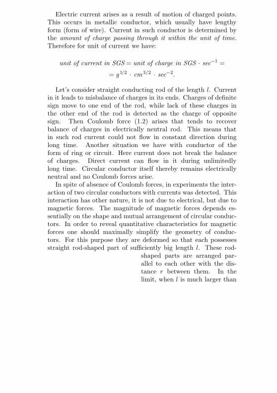
Choice of measure unit for electric charge in SGS is based onCoulomb law describing interaction of two charged point.

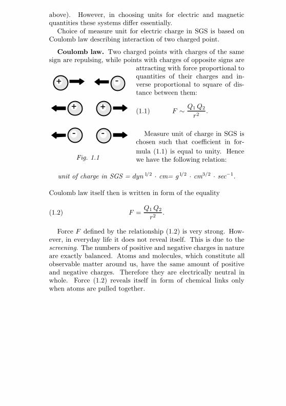
Coulomb law. Two charged points with charges of the samesign are repulsing, while points with charges of opposite signs are

attracting with force proportional toquantities of their charges and in-verse proportional to square of dis-tance between them:

(1.1) F ∼ Q1Q2

r2.

Measure unit of charge in SGS ischosen such that coefficient in for-

Fig. 1.1mula (1.1) is equal to unity. Hencewe have the following relation:

unit of charge in SGS = dyn 1/2 · cm= g 1/2 · cm3/2 · sec−1.

Coulomb law itself then is written in form of the equality

(1.2) F =Q1Q2

r2.

Force F defined by the relationship (1.2) is very strong. How-ever, in everyday life it does not reveal itself. This is due to thescreening. The numbers of positive and negative charges in natureare exactly balanced. Atoms and molecules, which constitute allobservable matter around us, have the same amount of positiveand negative charges. Therefore they are electrically neutral inwhole. Force (1.2) reveals itself in form of chemical links onlywhen atoms are pulled together.

Electric current arises as a result of motion of charged points.This occurs in metallic conductor, which usually have lengthyform (form of wire). Current in such conductor is determined bythe amount of charge passing through it within the unit of time.Therefore for unit of current we have:

unit of current in SGS = unit of charge in SGS · sec−1 =

= g 1/2 · cm 3/2 · sec−2.

Let’s consider straight conducting rod of the length l. Currentin it leads to misbalance of charges in its ends. Charges of definitesign move to one end of the rod, while lack of these charges inthe other end of the rod is detected as the charge of oppositesign. Then Coulomb force (1.2) arises that tends to recoverbalance of charges in electrically neutral rod. This means thatin such rod current could not flow in constant direction duringlong time. Another situation we have with conductor of theform of ring or circuit. Here current does not break the balanceof charges. Direct current can flow in it during unlimitedlylong time. Circular conductor itself thereby remains electricallyneutral and no Coulomb forces arise.

In spite of absence of Coulomb forces, in experiments the inter-action of two circular conductors with currents was detected. Thisinteraction has other nature, it is not due to electrical, but due tomagnetic forces. The magnitude of magnetic forces depends es-sentially on the shape and mutual arrangement of circular conduc-tors. In order to reveal quantitative characteristics for magneticforces one should maximally simplify the geometry of conduc-tors. For this purpose they are deformed so that each possessesstraight rod-shaped part of sufficiently big length l. These rod-

shaped parts are arranged par-allel to each other with the dis-tance r between them. In thelimit, when l is much larger than

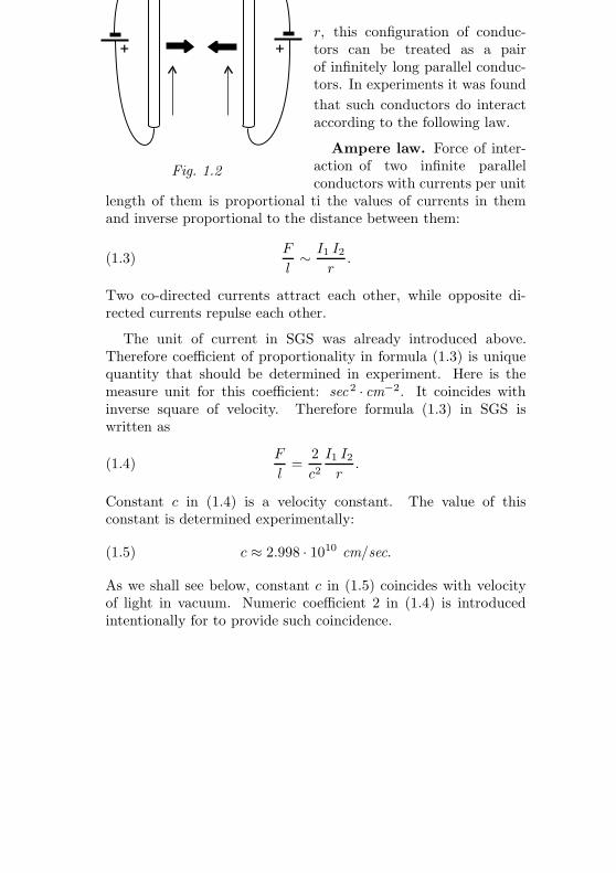
r, this configuration of conduc-tors can be treated as a pairof infinitely long parallel conduc-tors. In experiments it was found

Fig. 1.2

that such conductors do interactaccording to the following law.

Ampere law. Force of inter-action of two infinite parallelconductors with currents per unit

length of them is proportional ti the values of currents in themand inverse proportional to the distance between them:

(1.3)F

l∼ I1 I2

r.

Two co-directed currents attract each other, while opposite di-rected currents repulse each other.

The unit of current in SGS was already introduced above.Therefore coefficient of proportionality in formula (1.3) is uniquequantity that should be determined in experiment. Here is themeasure unit for this coefficient: sec 2 · cm−2. It coincides withinverse square of velocity. Therefore formula (1.3) in SGS iswritten as

(1.4)F

l=

2c2I1 I2r

.

Constant c in (1.4) is a velocity constant. The value of thisconstant is determined experimentally:

(1.5) c ≈ 2.998 · 1010 cm/sec.

As we shall see below, constant c in (1.5) coincides with velocityof light in vacuum. Numeric coefficient 2 in (1.4) is introducedintentionally for to provide such coincidence.

In SI measure unit of current 1 A (one ampere) is a basic unit.It is determined such that formula (1.3) is written as

(1.6)F

l=

2µ0

4πI1 I2r

.

Here π = 3.14 . . . is exact (though it is irrational) mathematicalconstant with no measure unit. Constant µ0 is called magneticsusceptibility of vacuum. It has the measure unit:

(1.7) µ0 = 4π · 10−7N · A−2.

But, in contrast to constant c in (1.5), it is exact constant. Itsvalue should not be determined experimentally. One could chooseit to be equal to unity, but the above value (1.7) for this constantwas chosen by convention when SI system was established. Dueto this value of constant (1.7) current of 1 ampere appears tobe in that range of currents, that really appear in industrial andhousehold devices. Coefficient 4π in denominator (1.6) is used inorder to simplify some other formulas, which are more often usedfor engineering calculations in electric technology.

Being basic unit in SI, unit of current ampere is used fordefining unit of charge of 1 coulomb: 1C = 1A · 1sec. Thencoefficient of proportionality in Coulomb law (1.1) appears to benot equal to unity. In SI Coulomb law is written as

(1.8) F =1

4πε0Q1Q2

r2.

Constant ε0 is called dielectric permittivity of vacuum. In con-trast to constant µ0 in (1.7) this is physical constant determinedexperimentally:

(1.9) ε0 ≈ 8.85 · 10−12 C 2 · N−1 · m−2.

Constants (1.5), (1.7), and (1.9) are related to each other by thefollowing equality:

(1.10) c =1√ε0 µ0

≈ 2.998 · 108 m/sec.

From the above consideration we see that SGS and SI systemsdiffer from each other not only in the scale of units, but in for-mulas for two fundamental laws: Coulomb law and Ampere law.SI better suits for engineering calculations. However, derivationof many formulas in this system appears more huge than in SGS.Therefore below in this book we use SGS system.

Comparing Coulomb law and Ampere law we see that electricaland magnetic forces reveal themselves in quite different way.However, they have common origin: they both are due to electriccharges. Below we shall see that their relation is much moreclose. Therefore theories of electricity and magnetism are usuallyunited into one theory of electromagnetic phenomena. Theory ofelectromagnetism is a theory with one measurable constant: thisis light velocity c. Classical mechanics (without Newton’s theoryof gravitation) has no measurable constants. Newton’s theory ofgravitation has one constant:

(1.11) γ ≈ 6.67 · 10−8 cm3 · g−1 · sec−2.

This theory is based on Newton’s fourth law formulated as follows.

Universal law of gravitation. Two point masses attracteach other with the force proportional to their masses and in-verse proportional to the square of distance between them.

Universal law of gravitation is given by the same formula

(1.12) F = γM1M2

r2

in both systems: in SGS and in SI.

According to modern notion of nature classical mechanics andNewton’s theory of gravitation are approximate theories. Cur-rently they are replaced by special theory of relativity and generaltheory of relativity. Historically they appeared as a result ofdevelopment of the theory of electromagnetism. Below we keepthis historical sequence in explaining all three theories.

Exercise 1.1. On the base of above facts find quantitative re-lation of measure units for charge and current in SGS and SI.

§ 2. Concept of near action.

Let’s consider pair of charged bodies, which are initially fixed,and let’s do the following mental experiment with them. Whenwe start moving second body apart from first one, the distance rbegins increasing and consequently force of Coulomb interaction(1.2) will decrease. In this situation we have natural question:how soon after second body starts moving second body will feelchange of Coulomb force of interaction ? There are two possibleanswers to this question:

(1) immediately;(2) with some delay depending on the distance between bodies.

First answer is known as concept of distant action. Taking thisconcept we should take formula (1.2) as absolutely exact formulaapplicable for charges at rest and for moving charges as well.

Second answer is based on the concept of near action. Ac-cording to this concept, each interaction (and electric interactionamong others) can be transmitted immediately only to the pointof space infinitesimally close to initial one. Transmission of anyaction to finite distance should be considered as a process ofsuccessive transmission from point to point. This process alwaysleads to some finite velocity of transmission for any action. Inthe framework of the concept of near action Coulomb law (1.2) istreated as approximate law, which is exact only for the charges

at rest that stayed at rest during sufficiently long time so thatprocess of transmission of electric interaction has been terminated.

Theory of electromagnetism has measurable constant c (lightvelocity (1.5)), which is first pretender for the role of transmissionvelocity of electric and magnetic interactions. For this reasonelectromagnetic theory is much more favorable as compared toNewton’s theory of gravitation.

The value of light velocity is a very large quantity. If we settlean experiment of measuring Coulomb force at the distances of theorder of r ≈ 10 cm, for the time of transmission of interaction wewould get times of the order of t ≈ 3 · 10−10 sec. Experimentaltechnique of XIX-th century was unable to detect such a shortinterval of time. Therefore the problem of choosing concept couldnot be solved experimentally. In XIX-th century it was subject forcontests. The only argument against the concept of distant actionthat time, quite likely, was its straightness, its self-completeness,and hence its scarcity.

In present time concept of near action is commonly accepted.Now we have the opportunity for testing it experimentally in thescope of electromagnetic phenomena. Let’s study this conceptmore attentively. According to the concept of near action, processof transmitting interaction to far distance exhibits an inertia.Starting at one point, where moving charge is placed, for sometime this process exist in hidden form with no influence to bothcharges. In order to describe this stage of process we need tointroduce new concept. This concept is a field.

Field is a material entity able to fill the whole space and ableto act upon other material bodies transmitting mutual interactionof them.

The number of fields definitely known to scientists is not big.There are only four fundamental fields: strong field, weak field,electromagnetic field, and gravitational field. Strong and weakfields are very short distance fields, they reveal themselves onlyin atomic nuclei, in collisions and decay of elementary particles,

and in stellar objects of extremely high density, which are calledneutron stars. Strong and weak interactions and fields are notconsidered in this book.

There are various terms using the word field: vector field, tensorfield, spinor field, gauge field, and others. These are mathematicalterms reflecting some definite properties of real physical fields.

§ 3. Superposition principle.

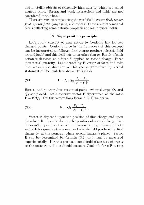
Let’s apply concept of near action to Coulomb law for twocharged points. Coulomb force in the framework of this conceptcan be interpreted as follows: first charge produces electric fieldaround itself, and this field acts upon other charge. Result of suchaction is detected as a force F applied to second charge. Forceis vectorial quantity. Let’s denote by F vector of force and takeinto account the direction of this vector determined by verbalstatement of Coulomb law above. This yields

(3.1) F = Q1Q2r2 − r1

|r2 − r1|3 .

Here r1 and r2 are radius-vectors of points, where charges Q1 andQ2 are placed. Let’s consider vector E determined as the ratioE = F/Q2. For this vector from formula (3.1) we derive

(3.2) E = Q1r2 − r1

|r2 − r1|3 .

Vector E depends upon the position of first charge and uponits value. It depends also on the position of second charge, butit doesn’t depend on the value of second charge. One can takevector E for quantitative measure of electric field produced by firstcharge Q1 at the point r2, where second charge is placed. VectorE can be determined by formula (3.2) or it can be measuredexperimentally. For this purpose one should place test charge qto the point r2 and one should measure Coulomb force F acting

upon this test charge. Then vector E is determined by division ofF by the value of test charge q:

(3.3) E = F/q.

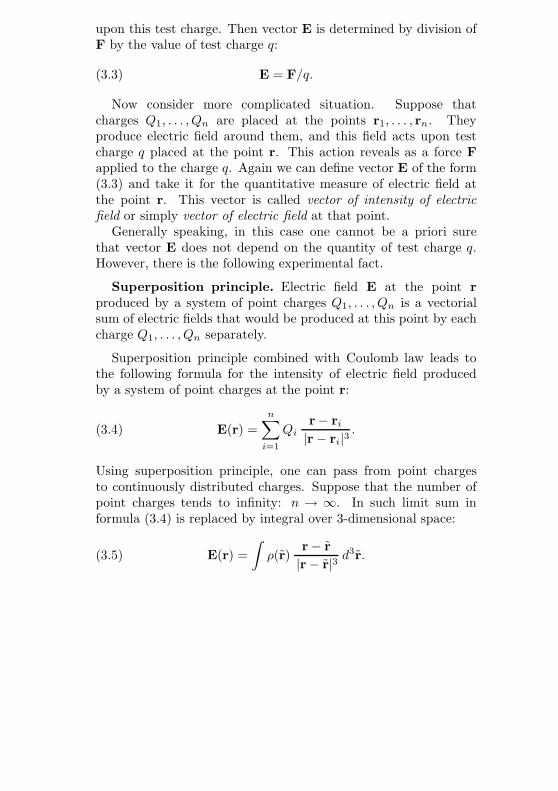
Now consider more complicated situation. Suppose thatcharges Q1, . . . , Qn are placed at the points r1, . . . , rn. Theyproduce electric field around them, and this field acts upon testcharge q placed at the point r. This action reveals as a force Fapplied to the charge q. Again we can define vector E of the form(3.3) and take it for the quantitative measure of electric field atthe point r. This vector is called vector of intensity of electricfield or simply vector of electric field at that point.

Generally speaking, in this case one cannot be a priori surethat vector E does not depend on the quantity of test charge q.However, there is the following experimental fact.

Superposition principle. Electric field E at the point rproduced by a system of point charges Q1, . . . , Qn is a vectorialsum of electric fields that would be produced at this point by eachcharge Q1, . . . , Qn separately.

Superposition principle combined with Coulomb law leads tothe following formula for the intensity of electric field producedby a system of point charges at the point r:

(3.4) E(r) =n∑

i=1

Qir− ri

|r− ri|3 .

Using superposition principle, one can pass from point chargesto continuously distributed charges. Suppose that the number ofpoint charges tends to infinity: n → ∞. In such limit sum informula (3.4) is replaced by integral over 3-dimensional space:

(3.5) E(r) =∫ρ(r)

r− r|r− r|3 d

3r.

Here ρ(r) is spatial density of charge at the point r. This valuedesignates the amount of charge per unit volume.

In order to find force acting on test charge q we should invertformula (3.3). As a result we obtain

(3.6) F = qE(r).

Force acting on a charge q in electric field is equal to the productof the quantity of this charge by the vector of intensity of field atthe point, where charge is placed. However, charge q also produceselectric field. Does it experience the action of its own field ? Forpoint charges the answer to this question is negative. This factshould be treated as a supplement to principle of superposition.Total force acting on a system of distributed charges in electricfield is determined by the following integral:

(3.7) F =∫ρ(r)E(r) d3r.

Field E(r) in (3.7) is external field produced by external charges.Field of charges with density ρ(r) is not included into E(r).

Concluding this section, note that formulas (3.4) and (3.5) holdonly for charges at rest, which stayed at rest for sufficiently longtime so that process of interaction transmitting reached the pointof observation r. Fields produced by such systems of charges arecalled static fields, while branch of theory of electromagnetismstudying such fields is called electrostatics.

§ 4. Lorentz force and Biot-Savart-Laplace law.

Ampere law of interaction of parallel conductors with currentsis an analog of Coulomb law for magnetic interactions. Accord-

ing to near action principle, force Farises as a result of action of mag-netic field produced by a current in

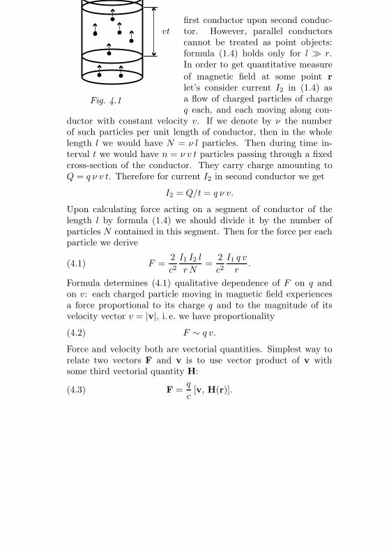
first conductor upon second conduc-tor. However, parallel conductorscannot be treated as point objects:formula (1.4) holds only for l r.In order to get quantitative measure

Fig. 4.1

vt

of magnetic field at some point rlet’s consider current I2 in (1.4) asa flow of charged particles of chargeq each, and each moving along con-

ductor with constant velocity v. If we denote by ν the numberof such particles per unit length of conductor, then in the wholelength l we would have N = ν l particles. Then during time in-terval t we would have n = ν v t particles passing through a fixedcross-section of the conductor. They carry charge amounting toQ = q ν v t. Therefore for current I2 in second conductor we get

I2 = Q/t = q ν v.

Upon calculating force acting on a segment of conductor of thelength l by formula (1.4) we should divide it by the number ofparticles N contained in this segment. Then for the force per eachparticle we derive

(4.1) F =2c2I1 I2 l

r N=

2c2I1 q v

r.

Formula determines (4.1) qualitative dependence of F on q andon v: each charged particle moving in magnetic field experiencesa force proportional to its charge q and to the magnitude of itsvelocity vector v = |v|, i. e. we have proportionality

(4.2) F ∼ q v.

Force and velocity both are vectorial quantities. Simplest way torelate two vectors F and v is to use vector product of v withsome third vectorial quantity H:

(4.3) F =q

c[v, H(r)].

Here c is scalar constant equal to light velocity. Vectorial quantityH(r) is a quantitative measure of magnetic field at the point r.It is called intensity of magnetic field at that point. Scalar factor1/c in (4.3) is used for to make H to be measured by the sameunits as intensity of electric field E in (3.6). Force F acting ona point charge in magnetic field is called Lorentz force. TotalLorentz force acting on a charge in electromagnetic field is a sumof two components: electric component and magnetic component:

(4.4) F = qE +q

c[v, H].

Formula (4.4) extends formula (3.6) for the case of general electro-magnetic fields. It holds not only for static but for time-dependent(non-static) fields. Surely the above derivation of formula (4.4) isempiric. Actually, one should treat formula (4.4) as experimentalfact that do not contradict to another experimental fact (1.4)within theory being developed.

Let’s turn back to our conductors. Formula (4.3) can beinterpreted in terms of currents. Each segment of unit length ofa conductor with current I in magnetic field H experiences theforce

(4.5)Fl

=I

c[τ , H]

acting on it. Here τ is unit vector tangent to conductor and di-rected along current in it. Total force acting on circular conductorwith current I is determined by contour integral

(4.6) F =∮I

c[τ (s), H(r(s))] ds,

where s is natural parameter on contour (length) and r(s) isvector-function determining shape of contour in parametric form.

Let’s consider the case of two parallel conductors. Force F nowcan be calculated by formula (4.5) assuming that first conductor

produces magnetic field H(r) that acts upon second conductor.Auxiliary experiment shows that vector H is perpendicular tothe plane of these two parallel conductors. The magnitude ofmagnetic field H = |H| can be determined by formula (4.1):

(4.7) H =2c

I1r.

Here r is the distance from observation point to the conductorproducing field at that point.

Magnetic field produced by conductor with current satisfiessuperposition principle. In particular, field of infinite straightline conductor (4.7) is composed by fields produced by separatesegments of this conductor. One cannot measure magnetic field ofseparate segment experimentally since one cannot keep constantcurrent is such separate segment for sufficiently long time. Buttheoretically one can consider infinitesimally small segment ofconductor with current of the length ds. And one can writeformula for magnetic field produced by such segment of conductor:

(4.8) dH(r) =1c

[I τ , r− r]|r− r|3 ds.

Here τ is unit vector determining spatial orientation of infinitesi-mal conductor. It is always taken to be directed along current I.In practice, when calculating magnetic fields produced by circularconductors, formula (4.8) is taken in integral form:

(4.9) H(r) =∮

1c

[I τ (s), r− r(s)]|r− r(s)|3 ds.

Like in (4.6), here s is natural parameter on the contour and r(s)is vectorial function determining shape of this contour. Thereforeτ (s) = dr(s)/ds. The relationship (4.8) and its integral form (4.9)constitute Biot-Savart-Laplace law for circular conductors withcurrent.

Biot-Savart-Laplace law in form (4.8) cannot be tested exper-imentally. However, in integral form (4.9) for each particularconductor it yields some particular expression for H(r). Thisexpression then can be verified in experiment.

Exercise 4.1. Using relationships (4.6) and (4.9), derive thelaw of interaction of parallel conductors with current in form (1.4).

Exercise 4.2. Find magnetic field of the conductor with cur-rent having the shape of circle of the radius a.

§ 5. Current densityand the law of charge conservation.

Conductors that we have considered above are kind of ideal-ization. They are linear, we assume them having no thickness.Real conductor always has some thickness. This fact is ignoredwhen we consider long conductors like wire. However, in somecases thickness of a conductor cannot be ignored. For example, ifwe consider current in electrolytic bath or if we study current inplasma in upper layers of atmosphere. Current in bulk conductorscan be distributed non-uniformly within volume of conductor.The concept of current density j is best one for describing suchsituation.

Current density is vectorial quantity depending on a point ofconducting medium: j = j(r). Vector of current density j(r)indicate the direction of charge transport at the point r. Itsmagnitude j = | j | is determined by the amount of charge passingthrough unit area perpendicular to vector j per unit time. Let’smark mentally some restricted domain Ω within bulk conductingmedium. Its boundary is smooth closed surface. Due to theabove definition of current density the amount of charge flowingout from marked domain per unit time is determined by surfaceintegral over the boundary of this domain, while charge enclosed

within this domain is given by spatial integral:

Q =∫Ω

ρ d3r, J =∫∂Ω

⟨j, n

⟩dS.(5.1)

Here n is unit vector of external normal to the surface ∂Ωrestricting domain Ω.

Charge conservation law is one more fundamental experimentalfact reflecting the nature of electromagnetism. In its classicalform it states that charges cannot appear from nowhere andcannot disappear as well, they can only move from one point toanother. Modern physics insert some correction to this statement:charges appear and can disappear in processes of creation andannihilation of pairs of elementary particles consisting of particleand corresponding antiparticle. However, even in such creation-annihilation processes total balance of charge is preserved sincetotal charge of a pair consisting of particle and antiparticle isalways equal to zero. When applied to integrals (5.1) chargeconservation law yields: Q = −J . This relationship means thatdecrease of charge enclosed within domain Ω is always due tocharge leakage through the boundary and conversely increase ofcharge is due to incoming flow through the boundary of thisdomain. Let’s write charge conservation law in the followingform:

(5.2)d

dt

( ∫Ω

ρ d3r)

+∫

∂Ω

⟨j, n

⟩dS = 0.

Current density j is a vector depending on a point of conductingmedium. Such objects in differential geometry are called vectorfields. Electric field E and magnetic field H are other examplesof vector fields. Surface integral J in (5.1) is called flow of vectorfield j through the surface ∂Ω. For smooth vector field any surface

integral like J can be transformed to spatial integral by means ofOstrogradsky-Gauss formula. When applied to (5.2), this yields

(5.3)∫Ω

(∂ρ

∂t+ div j

)d3r = 0.

Note that Ω in (5.3) is an arbitrary domain that we marked men-tally within conducting medium. This means that the expressionbeing integrated in (5.3) should be identically zero:

(5.4)∂ρ

∂t+ div j = 0.

The relationships (5.2) and (5.4) are integral and differentialforms of charge conservation law respectively. The relationship(5.4) also is known as continuity equation for electric charge.

When applied to bulk conductors with distributed current jwithin them, formula (4.6) is rewritten as follows:

(5.5) F =∫

1c

[ j(r), H(r)] d3r.

Biot-Savart-Laplace law for such conductors also is written interms of spatial integral in the following form:

(5.6) H(r) =∫

1c

[ j(r), r− r]|r− r|3 d3r.

In order to derive formulas (5.5) and (5.6) from formulas (4.6)and (4.8) one should represent bulk conductor as a union of linearconductors, then use superposition principle and pass to the limitby the number of linear conductors n→∞.

§ 6. Electric dipole moment.

Let’s consider some configuration of distributed charge withdensity ρ(r) which is concentrated within some restricted domainΩ. Let R be maximal linear size of the domain Ω. Let’s choosecoordinates with origin within this domain Ω and let’s chooseobservation point r which is far enough from the domain ofcharge concentration: |r| R. In order to find electric field E(r)produced by charges in Ω we use formula (3.5):

(6.1) E(r) =∫Ω

ρ(r)r− r|r− r|3 d

3r.

Since domain Ω in (6.1) is restricted, we have inequality |r| ≤ R.Using this inequality along with |r| R, we can write Taylorexpansion for the fraction in the expression under integration in(6.1). As a result we get power series in powers of ratio r/|r|:

(6.2)r− r|r− r|3 =

r|r|3 +

1|r|2 ·

(3

r|r| ·

⟨r|r| ,

r|r|⟩− r|r|)

+ . . . .

Substituting (6.2) into (6.1), we get the following expression for

the vector of electric field E(r) produced by charges in Ω:

(6.3) E(r) = Qr|r|3 +

3⟨r, D

⟩r− |r|2 D|r|5 + . . . .

First summand in (6.3) is Coulomb field of point charge Q placedat the origin, where Q is total charge enclosed in the domain Ω.It is given by integral (5.1).

Second summand in (6.3) is known as field of point dipoleplaced at the origin. Vector D there is called dipole moment. Forcharges enclosed within domain Ω it is given by integral

(6.4) D =∫Ω

ρ(r) r d3r.

For point charges dipole moment is determined by sum

(6.5) D =n∑

i=1

Qi ri.

For the system of charges concentrated near origin, which iselectrically neutral in whole, the field of point dipole

(6.6) E(r) =3⟨r, D

⟩r− |r|2 D|r|5

is leading term in asymptotics for electrostatic field (3.4) or(3.5) as r → ∞. Note that for the system of charges withQ = 0 dipole moment D calculated by formulas (6.4) and (6.5)is invariant quantity. This quantity remains unchanged whenwe move all charges to the same distance at the same directionwithout changing their mutual orientation: r→ r + r0.

Exercise 6.1. Concept of charge density is applicable to pointcharges as well. However, in this case ρ(r) is not ordinary function.It is distribution. For example point charge Q placed at the pointr = 0 is represented by density ρ(r) = Qδ(r), where δ(r) is Dirac’sdelta-function. Consider the density

(6.7) ρ(r) =⟨D, grad δ(r)

⟩=

3∑i=1

Di ∂δ(r)∂ri

.

Applying formula (5.1), calculate total charge Q corresponding tothis density (6.7). Using formula (6.4) calculate dipole momentfor distributed charge (6.7) and find electrostatic field producedby this charge. Compare the expression obtained with (6.6) andexplain why system of charges described by the above density (6.7)is called point dipole.

Exercise 6.2. Using formula (3.7) find the force acting onpoint dipole in external electric field E(r).

§ 7. Magnetic moment.

Let’s consider situation similar to that of previous section.Suppose some distributed system of currents is concentrated insome restricted domain near origin. Let R be maximal linearsize of this domain Ω. Current density j(r) is smooth vector-function, which is nonzero only within Ω and which vanishes atthe boundary ∂Ω and in outer space. Current density j(r) isassumed to be stationary, i. e. it doesn’t depend on time, and itdoesn’t break charge balance, i. e. ρ(r) = 0. Charge conservationlaw applied to this situation yields

(7.1) div j = 0.

In order to calculate magnetic field H(r) we use Biot-Savart-Laplace law written in integral form (5.6):

(7.2) H(r) =∫Ω

1c

[ j(r), r− r]|r− r|3 d3r.

Assuming that |r| R, we take Taylor expansion (6.2) andsubstitute it into (7.2). As a result we get

(7.3)

H(r) =∫Ω

[ j(r), r]c |r|3 d3r +

+∫Ω

3⟨r, r⟩[ j(r), r]− |r|2 [ j(r), r]

c |r|5 d3r + . . . .

Lemma 7.1. First integral in (7.3) is identically equal to zero.

Proof. Denote this integral by H1(r). Let’s choose somearbitrary constant vector e and consider scalar product

(7.4)⟨H1, e

⟩=∫Ω

⟨e, [ j(r), r]

⟩c |r|3 d3r =

∫Ω

⟨j(r), [ r, e]

⟩c |r|3 d3r.

Then define vector a and function f(r) as follows:

a =[r, e]c |r|3 , f(r) =

⟨a, r

⟩.

Vector a does not depend on r, therefore in calculating integral(7.4) we can take it for constant vector. For this vector we derive

a = grad f . Substituting this formula into the (7.4), we get

(7.5)

⟨H1, e

⟩=∫Ω

⟨j, grad f

⟩d3r =

=∫Ω

div(f j) d3r−∫Ω

f div j d3r.

Last integral in (7.5) is equal to zero due to (7.1). Previous inte-gral is transformed to surface integral by means of Ostrogradsky-Gauss formula. It is also equal to zero since j(r) vanishes at theboundary of domain Ω. Therefore

(7.6)⟨H1, e

⟩=∫∂Ω

f⟨j, n

⟩dS = 0.

Now vanishing of vector H1(r) follows from formula (7.6) since eis arbitrary constant vector. Lemma 7.1 is proved.

Let’s transform second integral in (7.3). First of all we denoteit by H2(r). Then, taking an arbitrary constant vector e, we formscalar product

⟨H2, e

⟩. This scalar product can be brought to

(7.7)⟨H2, e

⟩=

1c |r|5

∫Ω

⟨j(r), b(r)

⟩d3r,

where b(r) = 3⟨r, r⟩[r, e] − |r|2 [r, e]. If one adds gradient of

arbitrary function f(r) to b(r), this wouldn’t change integralin (7.7). Formulas (7.5) and (7.6) form an example of suchinvariance. Let’s specify function f(r), choosing it as follows:

(7.8) f(r) = −32⟨r, r⟩ ⟨

r, [r, e]⟩.

For gradient of function (7.8) by direct calculations we find

grad f(r) = −32⟨r, [r, e]

⟩r− 3

2⟨r, r⟩[r, e] =

= −3⟨r, r⟩[r, e]− 3

2(r⟨r, [r, e]

⟩− [r, e]⟨r, r⟩).

Now let’s use well-known identity [a, [b, c]] = b⟨a, c

⟩− c⟨a, b

⟩.

Assuming that a = r, b = r, and c = [r, e], we transform theabove expression for grad f to the following form:

(7.9) grad f(r) = −3⟨r, r⟩[r, e]− 3

2[r, [r, [r, e]]].

Right hand side of (7.9) contains triple vectorial product. In orderto transform it we use the identity [a, [b, c]] = b

⟨a, c

⟩− c⟨a, b

⟩again, now assuming that a = r, b = r, and c = e:

gradf(r) = −3⟨r, r⟩[r, e]− 3

2⟨r, e⟩[r, r] +

32|r|2 [r, e].

Let’s add this expression for gradf to vector b(r). Here isresulting new expression for this vector:

(7.10) b(r) = −32⟨r, e⟩[r, r] +

12|r|2 [r, e].

Let’s substitute (7.10) into formula (7.7). This yields

⟨H2, e

⟩=∫Ω

−3⟨r, e⟩ ⟨

r, [ j(r), r]⟩

+ |r|2 ⟨e, [ j(r), r]⟩

2 c |r|5 d3r.

Note that quantities j(r) and r enter into this formula in form of

vector product [ j(r), r] only. Denote by M the following integral:

(7.11) M =∫Ω

[r, j(r)]2 c

d3r.

Vector M given by integral (7.11) is called magnetic moment forcurrents with density j(r). In terms of M the above relationshipfor scalar product

⟨H2, e

⟩is written as follows:

(7.12)⟨H2, e

⟩=

3⟨r, e⟩ ⟨

r, M⟩− |r|2 ⟨e, M⟩|r|5 .

If we remember that e in formula (7.12) is an arbitrary constantvector, then from (7.3) and lemma 7.1 we can conclude that thefield of point magnetic dipole

(7.13) H(r) =3⟨r, M

⟩r− |r|2 M|r|5

is leading term in asymptotical expansion of static magnetic field(4.9) and (5.6) as r→∞.

Like electric dipole moment D of the system with zero totalcharge Q = 0, magnetic moment M is invariant with respectto displacements r → r + r0 that don’t change configuration ofcurrents within system. Indeed, under such displacement integral(7.11) is incremented by

(7.14) 4M =∫Ω

[r0, j(r)]2 c

d3r = 0.

Integral in formula (7.14) is equal to zero by the same reasons asin proof of lemma 7.1.

Exercise 7.1. Consider localized system of currents j(r) withcurrent density given by the following distribution:

(7.15) j(r) = −c [M, grad δ(r)].

Verify the relationship (7.1) for the system of currents (7.15) andfind its magnetic moment M. Applying formula (5.6), calculatemagnetic field of this system of currents and explain why this sys-tem of currents is called point magnetic dipole.

Exercise 7.2. Using formula (5.5), find the force acting uponpoint magnetic dipole in external magnetic field H(r).

Exercise 7.3. By means of the following formula for the torque

M =∫

1c

[r, [ j(r), H]] d3r

find torque M acting upon point magnetic dipole (7.15) in homo-geneous magnetic field H = const.

§ 8. Integral equationsfor static electromagnetic field.

Remember that we introduced the concept of flow of vectorfield through a surface in considering charge conservation law (seeintegral J in (5.1)). Now we consider flows of vector fields E(r)and H(r), i. e. for electric field and magnetic field:

E =∫S

⟨E, n

⟩dS, H =

∫S

⟨H, n

⟩dS.(8.1)

Let S be closed surface enveloping some domain Ω, i. e. S =∂Ω. Electrostatic field E is determined by formula (3.5). Let’s

substitute (3.5) into first integral (8.1) and then let’s change orderof integration in resulting double integral:

(8.2) E =∫ρ(r)

∫∂Ω

⟨r− r, n(r)

⟩|r− r|3 dS d3r.

Inner surface integral in (8.2) is an integral of explicit function.This integral can be calculated explicitly:

(8.3)∫

∂Ω

⟨r− r, n(r)

⟩|r− r|3 dS =

0, if r 6∈ Ω,4π, if r ∈ Ω.

Here by Ω = Ω ∪ ∂Ω we denote closure of the domain Ω.In order to prove the relationship (8.3) let’s consider vector

field m(r) given by the following formula:

(8.4) m(r) =r− r|r− r|3 .

Vector field m(r) is smooth everywhere except for one specialpoint r = r. In all regular points of this vector field by directcalculations we find div m = 0. If r 6∈ Ω special point of the fieldm is out of the domain Ω. Therefore in this case we can applyOstrogradsky-Gauss formula to (8.3):∫

∂Ω

⟨m, n

⟩dS =

∫Ω

div m d3r = 0.

This proves first case in formula (8.3). In order to prove secondcase, when r ∈ Ω, we use tactical maneuver. Let’s consider spher-ical ε-neighborhood O = Oε of special point r = r. For sufficientlysmall ε this neighborhood O = Oε is completely enclosed into the

domain Ω. Then from zero divergency condition div m = 0 forthe field given by formula (8.4) we derive

(8.5)∫

∂Ω

⟨m, n

⟩dS =

∫∂O

⟨m, n

⟩dS = 4π.

The value of last integral over sphere ∂O in (8.5) is found by directcalculation, which is not difficult. Thus, formula (8.3) is proved.Substituting (8.3) into (8.2) we get the following relationship:

(8.6)∫

∂Ω

⟨E, n

⟩dS = 4π

∫Ω

ρ(r) d 3r.

This relationship (8.6) can be formulated as a theorem.

Theorem (on the flow of electric field). Flow of electric fieldthrough the boundary of restricted domain is equal to total chargeenclosed within this domain multiplied by 4π.

Now let’s consider flow of magnetic field H in (8.1). Staticmagnetic field is determined by formula (5.6). Let’s substituteH(r) given by (5.6) into second integral (8.1), then change theorder of integration in resulting double integral:

(8.7) H =∫ ∫

∂Ω

1c

⟨[ j(r), r− r], n(r)

⟩|r− r|3 dS d 3r.

It’s clear that in calculating inner integral over the surface ∂Ωvector j can be taken for constant. Now consider the field

(8.8) m(r) =[ j, r− r]c |r− r|3 .

Like (8.4), this vector field (8.8) has only one singular point r = r.Divergency of this field is equal to zero, this fact can be verified

by direct calculations. As appears in this case, singular pointmakes no effect to the value of surface integral in (8.7). Insteadof (8.3) in this case we have the following formula:

(8.9)∫

∂Ω

1c

⟨[ j, r− r], n(r)

⟩|r− r|3 dS = 0.

For r 6∈ Ω the relationship (8.9) follows from divm = 0 byapplying Ostrogradsky-Gauss formula. For r ∈ Ω we have therelationship similar to the above relationship (8.5):

(8.10)∫

∂Ω

⟨m, n

⟩dS =

∫∂O

⟨m, n

⟩dS = 0.

However, the value of surface integral over sphere ∂O in this caseis equal to zero since vector m(r) is perpendicular to normalvector n at all points of sphere ∂O. As a result of substituting(8.9) into (8.7) we get the relationship

(8.11)∫

∂Ω

⟨H, n

⟩dS = 0,

which is formulated as the following theorem.

Theorem (on the flow of magnetic field). Total flow of mag-netic field through the boundary of any restricted domain is equalto zero.

Let r(s) be vectorial parametric equation of some closed spatialcurve Γ being the rim for some open surface S, i. e. Γ = ∂S. Opensurface S means that S and Γ have empty intersection. By S wedenote the closure of the surface S. Then S = S ∪ Γ. Takings for natural parameter on Γ, we define circulation for electric

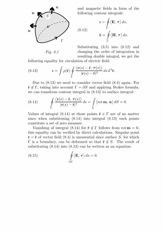
and magnetic fields in form of thefollowing contour integrals:

(8.12)

e =∮Γ

⟨E, τ

⟩ds,

h =∮Γ

⟨H, τ

⟩ds.

Substituting (3.5) into (8.12) andchanging the order of integration inFig. 8.1

Γ

n

Sn

n

resulting double integral, we get thefollowing equality for circulation of electric field:

(8.13) e =∫ρ(r)

∮Γ

⟨r(s)− r, τ (s)

⟩|r(s)− r|3 ds d 3r.

Due to (8.13) we need to consider vector field (8.4) again. Forr 6∈ Γ, taking into account Γ = ∂S and applying Stokes formula,we can transform contour integral in (8.13) to surface integral:

(8.14)∮Γ

⟨r(s)− r, τ (s)

⟩|r(s)− r|3 ds =

∫S

⟨rotm, n

⟩dS = 0.

Values of integral (8.14) at those points r ∈ Γ are of no mattersince when substituting (8.14) into integral (8.13) such pointsconstitute a set of zero measure.

Vanishing of integral (8.14) for r 6∈ Γ follows from rotm = 0,this equality can be verified by direct calculations. Singular pointr = r of vector field (8.4) is unessential since surface S, for whichΓ is a boundary, can be deformed so that r 6∈ S. The result ofsubstituting (8.14) into (8.13) can be written as an equation:

(8.15)∮∂S

⟨E, τ

⟩ds = 0.

Theorem (on the circulation of electric field). Total circula-tion of static electric field along the boundary of any restrictedopen surface is equal to zero.

Formula like (8.15) is available for magnetic field as well. Hereis this formula that determines circulation of magnetic field:

(8.16)∮∂S

⟨H, τ

⟩ds =

4 πc

∫S

⟨j, n

⟩dS.

Corresponding theorem is stated as follows.

Theorem (on the circulation of magnetic field). Circulation ofstatic magnetic field along boundary of restricted open surface isequal to total electric current penetrating this surface multipliedby fraction 4 π/c.

Integral over the surface S now is in right hand side of formula(8.16) explicitly. Therefore surface spanned over the contour Γnow is fixed. We cannot deform this surface as we did abovein proving theorem on circulation of electric field. This leads tosome technical complication of the proof. Let’s consider ε-blow-up of surface S. This is domain Ω(ε) being union of all ε-ballssurrounding all point r ∈ S. This domain encloses surface S andcontour Γ = ∂S. If ε→ 0, domain Ω(ε) contracts to S.

Denote by D(ε) = R3 \ Ω(ε) exterior of the domain Ω(ε) andthen consider the following modification of formula (5.6) thatexpresses Biot-Savart-Laplace law for magnetic field:

(8.17) H(r) = limε→0

∫D(ε)

1c

[ j(r), r− r]|r− r|3 d 3r.

Let’s substitute (8.17) into integral (8.12) and change the order ofintegration in resulting double integral. As a result we get

(8.18) h = limε→0

∫D(ε)

∮Γ

1c

⟨[ j(r), r(s)− r], τ (s)

⟩|r(s) − r|3 ds d 3r.

In inner integral in (8.18) we see vector field (8.8). Unlike vectorfiled (8.4), rotor of this field is nonzero:

(8.19) rotm =3⟨r− r, j

⟩(r− r)− |r− r|2 jc |r− r|5 .

Using Stokes formula and taking into account (8.19), we cantransform contour integral (8.18) to surface integral:∮

Γ

1c

⟨[ j(r), r(s)− r], τ (s)

⟩|r(s)− r|3 ds =

=∫S

3⟨r− r, j(r)

⟩ ⟨r− r, n(r)

⟩ − |r− r|2 ⟨ j(r), n(r)⟩

c |r− r|5 dS.

Denote by m(r) vector field of the following form:

m(r) =3⟨r− r, n(r)

⟩(r− r)− |r− r|2 n(r)c |r− r|5 .

In terms of the field m(r) formula for h is written as

h = limε→0

∫D(ε)

∫S

⟨m(r), j(r)

⟩dS d 3r.

Vector field m(r) in this formula has cubic singularity |r − r|−3

at the point r = r. Such singularity is not integrable in R3 (ifwe integrate with respect to d 3r). This is why we use auxiliarydomain D(ε) and limit as ε→ 0.

Let’s change the order of integration in resulting double integralfor circulation h. This leads to formula∫

S

∫D(ε)

⟨m(r), j(r)

⟩d 3r dS =

∫S

∫D(ε)

⟨gradf(r), j(r)

⟩d 3r dS,

since vector field m(r) apparently is gradient of the function f(r):

(8.20) f(r) = −⟨r− r, n(r)

⟩c |r− r|3 .

Function f(r) vanishes as r → ∞. Assume that current densityalso vanishes as r → ∞. Then due to the same considerations asin proof of lemma 7.1 and due to formula (7.1) spatial integral inthe above formula can be transformed to surface integral:

(8.21) h = limε→0

∫S

∫∂D(ε)

f(r)⟨j(r), n(r)

⟩dS dS.

Let’s change the order of integration in (8.21) then take intoaccount common boundary ∂D(ε) = ∂Ω(ε). Outer normal to thesurface ∂D(ε) coincides with inner normal to ∂Ω(ε). This coin-cidence and explicit form of function (8.20) lead to the followingexpression for circulation of magnetic field h:

(8.22) h = limε→0

∫∂Ω(ε)

⟨j(r), n(r)

⟩c

∫S

⟨r− r, n(r)

⟩|r− r|3 dS dS.

Let’s denote by V (r) inner integral in formula (8.22):

(8.23) V (r) =∫S

⟨r− r, n(r)

⟩|r− r|3 dS.

Integral (8.23) is well-known in mathematical physics. It is calledpotential of double layer. There is the following lemma, proof ofwhich can be found in [1].

Lemma 8.1. Double layer potential (8.23) is restricted func-tion in R3 \ S. At each inner point r ∈ S there are side limits

V±(r) = limr→±S

V (r),

inner limit V−(r) as r tends to r ∈ S from inside along normalvector n, and outer limit V+(r) as r tends to r ∈ S from outsideagainst the direction of normal vector n. Thereby V+ − V− = 4πfor all points r ∈ S.

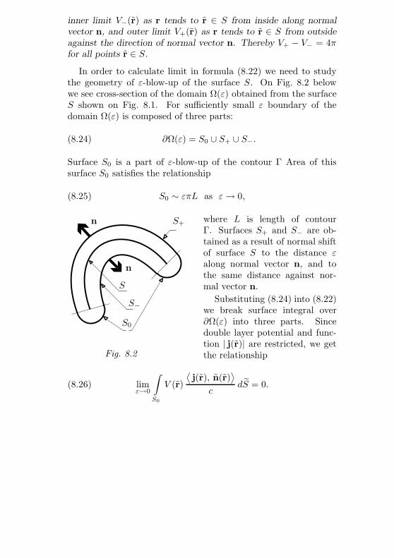
In order to calculate limit in formula (8.22) we need to studythe geometry of ε-blow-up of the surface S. On Fig. 8.2 belowwe see cross-section of the domain Ω(ε) obtained from the surfaceS shown on Fig. 8.1. For sufficiently small ε boundary of thedomain Ω(ε) is composed of three parts:

(8.24) ∂Ω(ε) = S0 ∪ S+ ∪ S−.

Surface S0 is a part of ε-blow-up of the contour Γ Area of thissurface S0 satisfies the relationship

(8.25) S0 ∼ επL as ε→ 0,

where L is length of contourΓ. Surfaces S+ and S− are ob-tained as a result of normal shiftof surface S to the distance εalong normal vector n, and tothe same distance against nor-mal vector n.

Fig. 8.2

S0

S−

S

n

n S+

Substituting (8.24) into (8.22)we break surface integral over∂Ω(ε) into three parts. Sincedouble layer potential and func-tion | j(r)| are restricted, we getthe relationship

(8.26) limε→0

∫S0

V (r)

⟨j(r), n(r)

⟩c

dS = 0.

For other two summand we also can calculate limits as ε→ 0:

(8.27)∫

S±

V (r)

⟨j(r), n(r)

⟩c

dS −→ ±∫S

V±(r)

⟨j(r), n(r)

⟩c

dS.

We shall not load reader with the proof of formulas (8.24), (8.25)and (8.27), which are sufficiently obvious. Summarizing (8.26)and (8.27) and taking into account lemma 8.1, we obtain

(8.28) h =4πc

∫S

⟨j(r), n(r)

⟩dS.

This relationship (8.28) completes derivation of formula (8.16)and proof of theorem on circulation of magnetic field in whole.

Exercise 8.1. Verify the relationship div m = 0 for vectorfields (8.4) and (8.8).

Exercise 8.2. Verify the relationship (8.19) for vector fieldgiven by formula (8.8).

Exercise 8.3. Calculate grad f for the function (8.20).

§ 9. Differential equationsfor static electromagnetic field.

In § 8 we have derived four integral equations for electric andmagnetic fields. They are used to be grouped into two pairs.Equations in first pair have zero right hand sides:

∫∂Ω

⟨H, n

⟩dS = 0,

∮∂S

⟨E, τ

⟩ds = 0.(9.1)

Right hand sides of equations in second pair are non-zero. Theyare determined by charges and currents:

(9.2)

∫∂Ω

⟨E, n

⟩dS = 4π

∫Ω

ρ d 3r,

∮∂S

⟨H, τ

⟩ds =

4 πc

∫S

⟨j, n

⟩dS.

Applying Ostrogradsky-Gauss formula and Stokes formula, onecan transform surface integrals to spatial ones, and contour inte-grals to surface integrals. Then, since Ω is arbitrary domain andS is arbitrary open surface, integral equations (9.1) and (9.2) can

be transformed to differential equations:

div H = 0, rotE = 0,(9.3)

div E = 4πρ, rotH =4πc

j.(9.4)

When considering differential equations (9.3) and (9.4), we shouldadd conditions for charges and currents being stationary:

∂ρ

∂t= 0,

∂j∂t

= 0.(9.5)

The relationship (7.1) then is a consequence of (9.5) and chargeconservation law.

Differential equations (9.3) and (9.4) form complete systemof differential equations for describing stationary electromagneticfields. When solving them functions ρ(r) and j(r) are assumed tobe known. If they are not known, one should have some additionalequations relating ρ and j with E and H. These additionalequations describe properties of medium (for instance, continuousconducting medium is described by the equation j = σE, where σis conductivity of medium).

CHAPTER II

CLASSICAL ELECTRODYNAMICS

§ 1. Maxwell equations.

Differential equations (9.3) and (9.4), which we have derivedin the end of Chapter I, describe fields generated by stationarycharges and currents. They are absolutely unsuitable if we aregoing to describe the process of haw electromagnetic interaction istransmitted in space. Note that the notion of field was introducedwithin framework of the concept of near action for describingthe object that transmit interaction of charges and currents. Forstatic fields this property is revealed in a very restrictive form,i. e. we use fields only to divide interaction of charges and currentsinto two processes: creation of a field by charges and currents isfirst process, action of this field upon other currents and chargesis second process. Dynamic properties of the field itself appearsbeyond our consideration.

More exact equations describing process of transmitting elec-tromagnetic interaction in its time evolution were suggested byMaxwell. They are the following ones:

div H = 0, rotE = −1c

∂H∂t

,(1.1)

div E = 4πρ, rotH =4πc

j +1c

∂E∂t.(1.2)

It is easy to see that equations (1.1) and (1.2) are generalizationsfor the (9.3) and (9.4) from Chapter I. They are obtained from

latter ones by modifying right hand sides. Like equations (9.3)and (9.4) in Chapter I, Maxwell equations (1.1) and (1.2) can bewritten in form of integral equations:∫

∂Ω

⟨H, n

⟩dS = 0,

∮∂S

⟨E, τ

⟩ds = −1

c

d

dt

∫S

⟨H, n

⟩dS,

(1.3)

∫∂Ω

⟨E, n

⟩dS = 4π

∫Ω

ρ d3r,

∮∂S

⟨H, τ

⟩ds =

4 πc

∫S

⟨j, n

⟩dS +

1c

d

dt

∫S

⟨E, n

⟩dS.

(1.4)

Consider contour integral in second equation (1.3). Similarcontour integral is present in second equation (1.4). However,unlike circulation of magnetic field, circulation of electric field

(1.5) e =∮∂S

⟨E, τ

⟩ds

possess its own physical interpretation. If imaginary contourΓ = ∂S in space is replaced by real circular conductor, thenelectric field with nonzero circulation induces electric current inconductor. The quantity e from (1.5) in this case is called electro-motive force of the field E in contour. Electromotive force e 6= 0in contour produce the same effect as linking electric cell withvoltage e into this contour. Experimentally it reveals as follow:alternating magnetic field produces electric field with nonzero cir-culation, this induces electric current in circular conductor. Thisphenomenon is known as electromagnetic induction. It was firstdiscovered by Faraday. Faraday gave qualitative description ofthis phenomenon in form of the following induction law.

Faraday’s law of electromagnetic induction. Electromo-tive force of induction in circular conductor is proportional to therate of changing of magnetic flow embraced by this conductor.

Faraday’s induction law was a hint for Maxwell when choosingright hand side in second equation (1.1). As for similar term inright hand side of second equation (1.2), Maxwell had written itby analogy. Experiments and further development of technologyproved correctness of Maxwell equations.

Note that charge conservation law in form of relationship (5.4)from Chapter I is a consequence of Maxwell equations. Oneshould calculate divergency of both sides of second equation (1.2):

div rotH =4πc

div j +1c

∂ div E∂t

,

then one should apply the identity div rotH = 0. When combinedwith the first equation (1.2) this yields exactly the relationship(5.4) from Chapter I.

Equations (1.1) and (1.2) form complete system for describ-ing arbitrary electromagnetic fields. In solving them functionsρ(r, t) and j(r, t) should be given, or they should be determinedfrom medium equations. Then each problem of electrodynam-ics mathematically reduces to some boundary-value problem ormixed initial-value/boundary-value problem for Maxwell equa-tions optionally completed by medium equations. In this section

we consider only some very special ones among such problems.Our main goal is to derive important mathematical consequencesfrom Maxwell equations and to interpret their physical nature.

§ 2. Density of energy and energy flowfor electromagnetic field.

Suppose that in bulk conductor we have a current with densityj, and suppose that this current is produced by the flow of chargedparticles with charge q. If ν is the number of such particles perunit volume and if v is their velocity, then j = q ν v. Recall thatcurrent density is a charge passing through unit area per unittime (see § 5 in Chapter I).

In electromagnetic field each particle experiences Lorentz forcedetermined by formula (4.4) from Chapter I. Work of this forceper unit time is equal to

⟨F, v

⟩= q

⟨E, v

⟩. Total work produced

by electromagnetic field per unit volume is obtained if one multi-plies this quantity by ν, then w = q ν

⟨E, v

⟩=⟨E, j

⟩. This work

increases kinetic energy of particles (particles are accelerated byfield). Otherwise this work is used for to compensate forces ofviscous friction that resist motion of particles. In either casetotal power spent by electromagnetic field within domain Ω isdetermined by the following integral:

(2.1) W =∫Ω

⟨E, j

⟩d3r.

Let’s transform integral (2.1). Let’s express current density jthrough E and H using second equation (1.2) for this purpose:

(2.2) j =c

4 πrotH− 1

4 π∂E∂t.

Substituting this expression (2.2) into formula (2.1), we get

(2.3) W =c

4 π

∫Ω

⟨E, rotH

⟩d3r− 1

8 π

∫Ω

∂

∂t

⟨E, E

⟩d3r.

In order to implement further transformations in formula (2.3)we use well-known identity div [a, b] =

⟨b, rota

⟩ − ⟨a, rotb⟩.

Assuming a = H and b = E, for W we get

W =c

4 π

∫Ω

div[H, E] d3r +c

4 π

∫Ω

⟨H, rotE

⟩d3r− d

dt

∫Ω

|E|28 π

d3r.

First integral in this expression can be transformed by means ofOstrogradsky-Gauss formula, while for transforming rotE one canuse Maxwell equations (1.1):

(2.4) W +∫∂Ω

c

4 π⟨[E, H], n

⟩dS +

d

dt

∫Ω

|E|2 + |H|28 π

d3r = 0.

Let’s denote by S and ε vectorial field and scalar field of the form

S =c

4 π[E,H], ε =

|E|2 + |H|28 π

.(2.5)

The quantity ε in (2.5) is called density of energy of electromag-netic field. Vector S is known as density of energy flow. It alsocalled Umov-Pointing vector. Under such interpretation of quan-tities (2.5) the relationship (2.4) can be treated as the equationof energy balance. First summand in (2.4) is called dissipationpower, this is the amount of energy dissipated per unit time atthe expense of transmitting it to moving charges. Second sum-mand is the amount of energy that flows from within domain Ω toouter space per unit time. These two forms of energy losses leadto diminishing the energy stored by electromagnetic field itselfwithin domain Ω (see third summand in (2.4)).

Energy balance equation (2.4) can be rewritten in differentialform, analogous to formula (5.4) from Chapter I:

(2.6)∂ε

∂t+ div S + w = 0.

Here w =⟨E, j

⟩is a density of energy dissipation. Note that in

some cases w and integral (2.1) in whole can be negative. In sucha case we have energy pumping into electromagnetic field. Thisenergy then flows to outer space through boundary of the domainΩ. This is the process of radiation of electromagnetic waves fromthe domain Ω. It is realized in antennas (aerials) of radio andTV transmitters. If we eliminate or restrict substantially theenergy leakage from the domain Ω to outer space, then we wouldhave the device like microwave oven, where electromagnetic fieldis used for transmitting energy from radiator to beefsteak.

Electromagnetic field can store and transmit not only theenergy, but the momentum as well. In order to derive momentumbalance equations let’s consider again the current with density jdue to the particles with charge q which move with velocity v.Let ν be concentration of these particles, i. e. number of particlesper unit volume. Then j = q ν v and ρ = q ν. Total force actingon all particles within domain Ω is given by integral

(2.7) F =∫Ω

ρE d3r +∫Ω

1c

[ j, H] d3r.

In order to derive formula (2.7) one should multiply Lorentz forceacting on each separate particle by the number of particles perunit volume ν and then integrate over the domain Ω.

Force F determines the amount of momentum transmittedfrom electromagnetic field to particles enclosed within domain Ω.Integral (2.7) is vectorial quantity. For further transformations ofthis integral let’s choose some constant unit vector e and considerscalar product of this vector e and vector F:

(2.8)⟨F, e

⟩=∫Ω

ρ⟨E, e

⟩d3r +

∫1c

⟨e, [ j, H]

⟩d3r.

Substituting (2.2) into (2.8), we get

(2.9)

⟨F, e

⟩=∫Ω

ρ⟨E, e

⟩d3r +

14 π

∫Ω

⟨e, [rotH, H]

⟩d3r−

− 14 π c

∫Ω

⟨e, [∂E/∂t, H]

⟩d3r.

Recalling well-known property of mixed product, we do cyclictransposition of multiplicands in second integral (2.9). Moreover,we use obvious identity [∂E/∂t, H] = ∂ [E, H] /∂t − [E, ∂H/∂t].This yields the following expression for

⟨F, e

⟩:⟨

F, e⟩

=∫Ω

ρ⟨E, e

⟩d3r +

14 π

∫Ω

⟨rotH, [H, e]

⟩d3r−

− 14 π c

d

dt

∫Ω

⟨e, [E, H]

⟩d3r +

14 π c

∫Ω

⟨e, [E, ∂H/∂t]

⟩d3r.

Now we apply second equation of the system (1.1) written as∂H/∂t = −c rotE. Then we get formula

(2.10)

⟨F, e

⟩+d

dt

∫Ω

⟨e, [E, H]

⟩4 π c

d3r =∫Ω

ρ⟨E, e

⟩d3r+

+∫Ω

⟨rot H, [H, e]

⟩+⟨rot E, [E, e]

⟩4 π

d3r.

In order to transform last two integrals in (2.10) we use thefollowing three identities, two of which we already used earlier:

(2.11)

[a, [b, c]] = b⟨a, c

⟩− c⟨a, b

⟩,

div [a, b] =⟨b, rot a

⟩− ⟨a, rot b⟩,

rot [a, b] = a div b− b div a− a, b.

Here by curly brackets we denote commutator of two vectorfields a and b (see [2]). Traditionally square brackets are usedfor commutator, but here by square brackets we denote vectorproduct of two vectors. From second identity (2.11) we derive⟨

rotH, [H, e]⟩

= div [H, [H, e]] +⟨H, rot [H, e]

⟩.

In order to transform rot[H, e] we use third identity (2.11):rot[H, e] = −e div H− H, e. Then

⟨H, rot [H, e]

⟩= −⟨H, e⟩ div H +

3∑i=1

Hi

3∑j=1

ej ∂Hi

∂rj=

= −⟨H, e⟩ div H +12⟨e, grad |H|2⟩.

Let’s combine two above relationships and apply first identity(2.11) for to transform double vectorial product [H, [H, e]] infirst of them. As a result we obtain⟨

rotH, [H, e]⟩

= div(H⟨H, e

⟩)− div(e |H|2)−

− ⟨H, e⟩ div H +12⟨e, grad |H|2⟩.

But div(e |H|2)= ⟨e, grad |H|2⟩. Hence as a final result we get

(2.12)

⟨rotH, [H, e]

⟩= −⟨H, e⟩ div H+

+ div(H⟨H, e

⟩− 12

e |H|2).

Quite similar identity can be derived for electric field E:

(2.13)

⟨rotE, [E, e]

⟩= −⟨E, e⟩ div E+

+ div(E⟨E, e

⟩− 12

e |E|2).

The only difference is that due to Maxwell equations div H = 0,while divergency of electric field E is nonzero: div E = 4πρ.

Now, if we take into account (2.12) and (2.13), formula (2.10)can be transformed to the following one:

⟨F, e

⟩− ∫∂Ω

⟨E, e

⟩⟨n, E

⟩+⟨H, e

⟩⟨n, H

⟩4 π

dS+

+∫

∂Ω

(|E|2 + |H|2) ⟨e, n⟩8 π

dS +d

dt

∫Ω

⟨e, [E, H]

⟩4 π c

d3r = 0.

Denote by σ linear operator such that the result of applying this

operator to some arbitrary vector e is given by formula

(2.14) σ e = −E⟨E, e

⟩+ H

⟨H, e

⟩4 π

+|E|2 + |H|2

8 πe.

Formula (2.14) defines tensorial field σ of type (1, 1) with thefollowing components:

(2.15) σij =

|E|2 + |H|28 π

δij −

Ei Ej +Hi Hj

4 π.

Tensor σ with components (2.15) is called tensor of the densityof momentum flow. It is also known as Maxwell tensor. Now let’sdefine vector of momentum density p by formula

(2.16) p =[E, H]4 π c

.

In terms of the notations (2.15) and (2.16) the above relationshipfor⟨F, e

⟩is rewritten as follows:

(2.17)⟨F, e

⟩+∫

∂Ω

⟨σ e, n

⟩dS +

d

dt

∫Ω

⟨p, e

⟩d3r = 0.

Operator of the density of momentum flow σ is symmetric, i. e.⟨σ e, n

⟩=⟨e, σ n

⟩. Due to this property and because e is

arbitrary vector we can rewrite (2.17) in vectorial form:

(2.18) F +∫

∂Ω

σ n dS +d

dt

∫Ω

p d3r = 0.

This equation (2.18) is the equation of momentum balance forelectromagnetic field. Force F, given by formula (2.7) determinesloss of momentum stored in electromagnetic field due to transmit-ting it to moving particles. Second term in (2.18) determines loss

of momentum due to its flow through the boundary of the domainΩ. These two losses lead to diminishing the momentum storedby electromagnetic field within domain Ω (see third summand in(2.18)).

The relationship (2.18) can be rewritten in differential form.For this purpose we should define vectorial divergency for tensorialfield σ of the type (1, 1). Let

(2.19) µ = div σ, where µj =3∑

i=1

∂σij

∂ri.

Then differential form of (2.18) is written as

(2.20)∂p∂t

+ div σ + f = 0,

where f = ρE + [ j, H]/c is a density of Lorentz force, whilevectorial divergency is determined according to (2.19).

Thus, electromagnetic field is capable to accumulate withinitself the energy and momentum:

E =∫Ω

|E|2 + |H|28 π

d3r, P =∫Ω

[E, H]4 π c

d3r.(2.21)

It is also capable to transmit energy and momentum to materialbodies. This confirms once more our assertion that electromag-netic field itself is a material entity. It is not pure mathematicalabstraction convenient for describing interaction of charges andcurrents, but real physical object.

Exercise 2.1. Verify that relationships (2.11) hold. Check onthe derivation of (2.12) and (2.13).

§ 3. Vectorial and scalar potentialsof electromagnetic field.

In section 2 we have found that electromagnetic field possessenergy and momentum (2.21). This is very important conse-quence of Maxwell equations (1.1) and (1.2). However we havenot studied Maxwell equations themselves. This is system of fourequations, two of them are scalar equations, other two are vecto-rial equations. So they are equivalent to eight scalar equations.However we have only six undetermined functions in them: threecomponents of vector E and three components of vector H. Soobserve somewhat like excessiveness in Maxwell equations.

One of the most popular ways for solving systems of algebraicequations is to express some variable through other ones bysolving one of the equations in a system (usually most simpleequation) and then substituting the expression obtained into otherequations. Thus we exclude one variable and diminish the numberof equations in a system also by one. Sometimes this trickis applicable to differential equations as well. Let’s considerMaxwell equation div H = 0. Vector field with zero divergency iscalled vortex field. For vortex fields the following theorem holds(see proof in book [3]).

Theorem on vortex field. Each vortex field is a rotor of someother vector field.

Let’s write the statement of this theorem as applied to mag-netic field. It is given by the following relationship:

(3.1) H = rotA.

Vector field A, whose existence is granted by the above theorem,is called vector-potential of electromagnetic field.

Let’s substitute vector H as given by (3.1) into second Maxwellequation (1.1). This yields the equality

(3.2) rotE +1c

∂

∂trotA = rot

(E +

1c

∂A∂t

)= 0.

Vector field with zero rotor is called potential field. It is vectorfield E + (∂A/∂t)/c in formula (3.2) which is obviously potentialfield. Potential fields are described by the following theorem (seeproof in book [3]).

Theorem on potential field. Each potential field is a gradi-ent of some scalar field.

Applying this theorem to vector field (3.2), we get the relation-ship determining scalar potential of electromagnetic field ϕ:

(3.3) E +1c

∂A∂t

= − gradϕ.

Combining (3.1) and (3.3), we can express electric and magneticfields E and H through newly introduced fields A and ϕ:

(3.4)E = − gradϕ− 1

c

∂A∂t

,

H = rotA.

Upon substituting (3.4) into first pair of Maxwell equations(1.1) we find them to be identically fulfilled. As for second pair ofMaxwell equations, substituting (3.4) into these equations, we get

(3.5)−4ϕ− 1

c

∂

∂tdiv A = 4 π ρ,

graddiv A−4A +1c

∂

∂tgradϕ+

1c2∂2A∂t2

=4 π jc.

In deriving (3.5) we used relationships

(3.6)div gradϕ = 4ϕ,rot rotA = graddiv A−4A.

Second order differential operator 4 is called Laplace operator. Inrectangular Cartesian coordinates it is defined by formula

(3.7) 4 =3∑

i=1

(∂

∂ri

)2

=∂2

∂x2+

∂2

∂y2+

∂2

∂z2.

In order to simplify the equations (3.5) we rearrange terms inthem. As a result we get

(3.8)

1c2∂2ϕ

∂t2−4ϕ = 4 π ρ+

1c

∂

∂t

(1c

∂ϕ

∂t+ div A

),

1c2∂2A∂t2

−4A =4 π jc− grad

(1c

∂ϕ

∂t+ div A

).

Differential equations (3.8) are Maxwell equations written interms of A and ϕ. This is system of two equations one ofwhich is scalar equation, while another is vectorial equation. Aswe can see, number of equations now is equal to the number ofundetermined functions in them.

§ 4. Gauge transformations and Lorentzian gauge.

Vectorial and scalar potentials A and ϕ were introduced in§ 3 as a replacement for electric and magnetic fields E and H.However, fields A and ϕ are not physical fields. Physical fieldsE and H are expressed through A and ϕ according to formulas(3.4), but backward correspondence is not unique, i. e. fields Aand ϕ are not uniquely determined by physical fields E and H.Indeed, let’s consider transformation

(4.1)A = A + gradψ,

ϕ = ϕ− 1c

∂ψ

∂t,

where ψ(r, t) is an arbitrary function. Substituting (4.1) intoformula (3.4), we immediately get

E = E, H = H.

This means that physical fields E, H determined by fields A, ϕand by fields A, ϕ do coincide. Transformation (4.1) that do notchange physical fields E and H is called gauge transformation.

We use gauge transformations (4.1) for further simplification ofMaxwell equations (3.8). Let’s consider the quantity enclosed inbrackets in right hand sides of the equations (3.8):

(4.2)1c

∂ϕ

∂t+ div A =

1c

∂ϕ

∂t+ div A +

(1c2∂2ψ

∂t2−4ψ

).

Denote by the following differential operator:

(4.3) =1c2∂2

∂t2−4.

Operator (4.3) is called d’Alambert operator or wave operator.Differential equation u = v is called d’Alambert equation.

Using gauge freedom provided by gauge transformation (4.1),we can fulfill the following condition:

(4.4)1c

∂ϕ

∂t+ div A = 0.

For this purpose we should choose ψ solving d’Alambert equation

ψ = −(

1c

∂ϕ

∂t+ div A

).

It is known that d’Alambert equation is solvable under ratherweak restrictions for its right hand side (see book [1]). Hencepractically always we can fulfill the condition (4.4). This conditionis called Lorentzian gauge.

If Lorentzian gauge condition (4.4) is fulfilled, then Maxwellequations (3.8) simplify substantially:

ϕ = 4 π ρ, A =4 π jc.(4.5)

They look like pair of independent d’Alambert equations. How-ever, one shouldn’t think that variables A and ϕ are completely

separated. Lorentzian gauge condition (4.4) itself is an additionalequation requiring concordant choice of solutions for d’Alambertequations (4.5).

D’Alambert operator (4.3) is a scalar operator, in (4.5) it actsupon each component of vector A separately. Therefore operator commutates with rotor operator and with time derivative aswell. Therefore on the base of (3.4) we derive

E = −4π gradρ− 4πc2

∂j

∂t, H =

4πc

rot j.(4.6)

These equations (4.6) have no entries of potentials A and ϕ.They are written in terms of real physical fields E and H, andare consequences of Maxwell equations (1.1) and (1.2). However,backward Maxwell equations do not follow from (4.6).

§ 5. Electromagnetic waves.

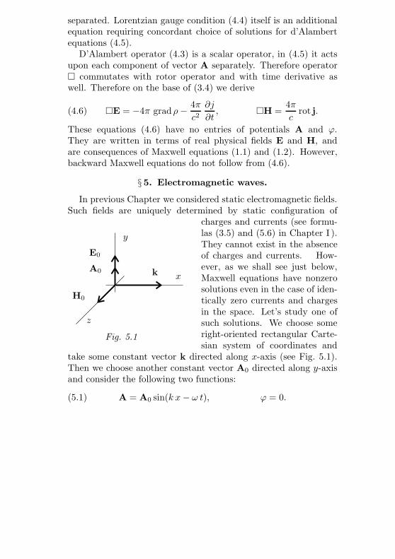
In previous Chapter we considered static electromagnetic fields.Such fields are uniquely determined by static configuration of

charges and currents (see formu-las (3.5) and (5.6) in Chapter I ).They cannot exist in the absenceof charges and currents. How-

Fig. 5.1

z

H0

xkA0

E0

y

ever, as we shall see just below,Maxwell equations have nonzerosolutions even in the case of iden-tically zero currents and chargesin the space. Let’s study one ofsuch solutions. We choose someright-oriented rectangular Carte-sian system of coordinates and

take some constant vector k directed along x-axis (see Fig. 5.1).Then we choose another constant vector A0 directed along y-axisand consider the following two functions:

A = A0 sin(k x− ω t), ϕ = 0.(5.1)

Here k = |k|. Suppose ρ = 0 and j = 0. Then, substituting (5.1)into (4.4) and into Maxwell equations (4.5), we get

(5.2) k2 = |k|2 =ω

c.

It is not difficult to satisfy this condition (5.2). If it is fulfilled,then corresponding potentials (5.1) describe plane electromag-netic wave, ω being its frequency and k being its wave-vector,which determines the direction of propagation of that plane wave.Rewriting (5.1) in a little bit different form

(5.3) A = A0 sin(k(x− c t)),

we see that the velocity of propagating of plane electromagneticwave is equal to constant c (see (1.5) in Chapter I).

Now let’s substitute (5.1) into (3.4) and calculate electric andmagnetic fields in electromagnetic wave:

E = E0 cos(k x− ω t), E0 = |k|A0,

H = H0 cos(k x− ω t), H0 = [k,A0],(5.4)

|E0| = |H0| = |k| |A0|.Vectors k, E0, and H0 are perpendicular to each other, they formright triple. Wave (5.4) with such vectors is called plane linearpolarized electromagnetic wave. Vector E0 is taken for polarizationvector of this wave. Wave

E = E0 cos(k x− ω t) + H0 sin(k x− ω t),

H = H0 cos(k x− ω t)−E0 sin(k x− ω t)

is called circular polarized wave. It is superposition of two linearpolarized waves. Natural light is also electromagnetic wave. Ithas no fixed polarization, however it is not circular polarized aswell. Natural light is a superposition of numerous plane linearpolarized waves with chaotically distributed polarization vectors.

§ 6. Emission of electromagnetic waves.

Plane wave (5.4) is an endless wave filling the whole space. Itis certainly kind of idealization. Real electromagnetic waves fillonly some restricted part of the space. Moreover, they are noteternal in time: there are sources (radiators) and absorbers ofelectromagnetic fields. Formula (5.4) is an approximate descrip-tion of real electromagnetic field in that part of space which is farapart from radiators and absorbers.

In this section we consider process of generation and radiationof electromagnetic waves. Usually radiator is a system of chargesand currents, which is not static. We describe it by means offunctions ρ(r, t) and j(r, t). Let’s consider Maxwell equationstransformed to the form (4.5). These are non-homogeneous differ-ential equations. Their solutions are not unique: to each solutionalready found one can add arbitrary solution of correspondinghomogeneous equations. However, if we assume ρ(r, t) and j(r, t)to be fast decreasing as r → ∞ and apply similar condition toϕ(r, t) and A(r, t), then we restrict substantially the freedom inchoosing solutions of the equations (4.5). In order to find oneof such solutions we need fundamental solution of d’Alambertoperator. This is distribution of the form:

(6.1) u(r, t) =c

2πθ(t) δ(c2t2 − |r|2),

where θ and δ are Heaviside theta-function and Dirac delta-function respectively. Function (6.1) satisfies d’Alambert equationwith distribution in right hand side:

u = δ(t)δ(r).

In physics such objects are called Green functions. Knowingfundamental solution (6.1) of d’Alambert operator, now we canwrite solution for the equations (4.5) in form of contractions:

ϕ = 4π u ∗ ρ, A =4πcu ∗ j.(6.2)

Here ∗ denotes contraction of two distributions, see [1]. Due tothe properties of this operation from charge conservation law (seeformula (5.4) in Chapter I) we derive Lorentzian gauge condition(4.4) for scalar and vectorial potentials (6.2). For smooth andsufficiently fast decreasing functions ρ(r, t) and j(r, t) potentials(6.2) are reduced to the following two integrals:

(6.3)

ϕ(r, t) =∫ρ(r, t− τ)|r− r| d3r,

A(r, t) =∫

j(r, t− τ)c |r− r| d

3r.

Here the quantity τ = τ(r, r) is called time delay. It is determinedby the ratio τ = |r − r|/c. Potentials (6.3) are called retardedpotentials.

Retarded potentials have transparent physical interpretation.Scalar potential ϕ at the point r at time instant t is a superposi-tion of contributions from charges at various points of the space,the contribution from the point r being determined not by chargedensity at present time instant t, but at previous time instantt − τ . Time delay τ is exactly equal to the time required for thesignal spreading with light velocity c from the source point r toget to the observation point r. Similar time delay is present informula for vector potential A.

Note that fundamental solution of d’Alambert equation is notunique. For example there is a solution obtained from (6.1)by changing τ for −τ . Such solution corresponds to advancedpotentials. However, in physics advanced potentials have nomeaning, since they would break causality principle.

Let’s consider system of charges located in some small domainΩ surrounding the origin. Let R be maximal linear size ofthis domain Ω. Using formulas (6.3), we calculate we calculateelectromagnetic field of the system of charges at the point r whichis far distant from the domain Ω, i. e. |r| ≤ R |r|. Due to these

inequalities the ratio r/|r| is small vectorial quantity. Thereforewe have the following asymptotic expansions for |r− r| and t− τ :

(6.4)

|r− r| = |r| −⟨r, r⟩

|r| + . . . ,

t− τ = t− |r|c

+

⟨r, r⟩

|r| c + . . . .

The ratio |r|/c in (6.4) determines the time required for electro-magnetic signal to get from the domain Ω to the observation point|r|. Posterior terms in the series for t− τ are estimated by smallquantity R/c. This is the time of propagation of electromagneticsignal within domain Ω.

Denote t′ = t− |r|/c and let t− τ = t′ + θ. For the quantity θwe have the estimate |θ| ≤ R/c. Then let’s consider the followingTaylor expansions for ρ and j:

(6.5)ρ(r, t− τ) = ρ(r, t′) +

∂ρ(r, t′)∂t

θ + . . . ,

j(r, t− τ) = j(r, t′) +∂j(r, t′)∂t

θ + . . . .

The condition R |r| is not sufficient for the expansions (6.5) tobe consistent. Use of expansions (6.5) for approximating ρ(r, t−τ)and j(r, t− τ) is possible only under some additional assumptionsconcerning these functions. Denote by T some specific time forwhich functions ρ and j within domain Ω change substantially. Incase when one can specify such time T , the following quantitiesare of the same order, i. e. equally large or equally small:

(6.6)ρ ≈ T

∂ρ

∂t≈ . . . ≈ T n ∂

nρ

∂tn,

j ≈ T∂j∂t≈ . . . ≈ T n ∂

nj∂tn

.

Now (6.5) can be rewritten as follows:

(6.7)ρ(r, t− τ) = ρ(r, t′) + T

∂ρ(r, t′)∂t

θ

T+ . . . ,

j(r, t− τ) = j(r, t′) + T∂j(r, t′)∂t

θ

T+ . . . .

Correctness of use of expansions (6.7) and (6.5) is provided byadditional condition R/c T . This yields θ/T 1.

The condition R/c T has simple meaning: the quantityω = 2π/T is a frequency of radiated electromagnetic waves, whileλ = 2πc/ω = c T is a wavelength. Hence condition R/c Tmeans that wavelength is mach greater than the size of radiator.

Suppose that both conditions R c T and R |r| are fulfilled.Let’s calculate retarded vector potential A in (6.3) keeping onlyfirst term in the expansion (6.5):

(6.8) A =∫Ω

j(r, t′)|r| c d3r + . . . .

In order to transform integral in (6.8) let’s choose some arbitraryconstant vector e and consider scalar product

⟨A, e

⟩. Having

defined vector a and function f(r) by the relationships

a =ec|r| = grad f, f(r) =

⟨a, r

⟩,

we make calculations analogous to that of (7.5) in Chapter I:

(6.9)

∫Ω

⟨j, gradf

⟩d3r =

∫Ω

div(f j) d3r−∫Ω

f div j d3r =

=∫∂Ω

f⟨j, n

⟩dS +

∫Ω

f∂ρ

∂td3r =

∫Ω

∂ρ(r, t′)∂t

⟨e, r

⟩|r| c d3r.

Since e is arbitrary vector, for vector potential A from (6.9) wederive the following formula:

(6.10) A =∫Ω

∂ρ(r, t′)∂t

r|r| c d

3r + . . . =D|r| c + . . . .

Here D = D(t′) is time derivative of dipole moment D of thesystem of charges at time instant t′.

In a similar way, keeping only initial terms in the expansions(6.4) and (6.5), for scalar potential ϕ in (6.3) we find

(6.11) ϕ =∫Ω

ρ(r, t′)|r| d3r + . . . =

Q

|r| + . . . ,

where Q is total charge enclosed within domain Ω. This chargedoes not depend on time since domain Ω is isolated and we haveno electric current in outer space.

Let’s compare the expressions under integration in (6.10) and(6.11) taking into account (6.6). This comparison yields

|A| ≈ R

cTϕ.

The estimate R/(c T ) 1 following from R c T means thatvectorial potential is calculated with higher accuracy than scalarpotential. Hence in calculating ϕ one should take into accounthigher order terms in expansions (6.4) and (6.5). Then

(6.12)

ϕ =Q

|r| +∫Ω

∂ρ(r, t′)∂t

⟨r, r⟩

|r|2 c d3r+

+∫Ω

ρ(r, t′)|r|

⟨r, r⟩

|r|2 d3r + . . . .

Calculating integrals in formula (6.12), we transform it to

(6.13) ϕ =Q

|r| +

⟨D, r

⟩|r|2 c +

⟨D, r

⟩|r|3 + . . . .

Potentials (6.10) and (6.13) are retarded potentials of thesystem of charges in dipole approximation. Dependence of ρ and jon time variable t lead to the dependence of D on t′ in them. Let’sconsider asymptotics of of these potentials as r → ∞. Therebywe can omit last term in (6.13). Then

ϕ =Q

|r| +

⟨D, r

⟩|r|2 c + . . . , A =

D|r| c + . . . .(6.14)

Now on the base of formulas (3.4) and (6.14) we findasymptotics of electric and magnetic fields at far distance from

the system of charges. In calculating rotA and gradϕ we takeinto account that t′ = t− |r|/c in argument of D(t′) is a quantitydepending on r. This dependence determines leading terms inasymptotics of E and H:

E =[r, [r, D]]|r|3 c2 + . . . , H = − [r, D]

|r|2 c2 + . . . .(6.15)

Vectors E and H (more precisely, leading terms in their asymp-totics) are perpendicular to each other and both are perpendicularto vector r. This situation is similar to that of plane wave. How-ever, in present case we deal with spherical wave being radiatedfrom the origin. The magnitude of fields |E| ' |H| decreases as1/|r|, which is slower than for static Coulomb field. Using formula(2.5), one can find the density of energy flow for waves (6.15):

(6.16) S =|[r, D]|24π |r|5 c3 r + . . . .

For modulus of vector S we have |S| ∼ 1/|r|2. This means thattotal flow of energy through the sphere of arbitrarily large sphereis nonzero. So we have real radiation of electromagnetic energy.The amount of radiated energy is determined by second timederivative of dipole moment. Therefore this case is called dipoleapproximation in theory of radiation.

Exercise 6.1. Applying formula (6.16), find angular distribu-tion of the intensity for dipole radiation. Also find total intensityof dipole radiation.

Exercise 6.2. Particle with charge q is moving along circularpath of radius R with constant velocity v = ωR for infinitely longtime (ω is angular velocity). Calculate retarding potentials andfind angular distribution for intensity of electromagnetic radiationof this particle. Also find total intensity of such cyclotronic radia-tion.

Exercise 6.3. Assume that charge density ρ is zero, while cur-rent density j is given by the following distribution:

(6.17) j(r, t) = −c [M(t), grad δ(r)]

(compare with (7.16) in Chapter I). Find retarding potentials (6.2)for (6.17). Also find angular distribution and total intensity formagnetic-dipole radiation induced by current (6.17).

CHAPTER III

SPECIAL THEORY OF RELATIVITY

§ 1. Galileo transformations.

Classical electrodynamics based on Maxwell equations histor-ically was first field theory. It explained all electromagneticphenomena and predicted the existence of electromagnetic waves.Later on electromagnetic waves were detected experimentally andnowadays they have broad scope of applications in our everydaylife. However, along with successful development of this theory,some difficulties there appeared. It was found that classical elec-trodynamics contradicts to relativity principle. This principle inits classical form suggested by Galileo and Newton states thattwo Cartesian inertial coordinate systems moving with constantvelocity with respect to each other are equivalent. All physi-cal phenomena in these two systems happen identically and aredescribed by the same laws.

Let’s consider two such Cartesian inertial coordinate systems(r, t) and (r, t). Suppose that second system moves with velocityu relative to first one so that coordinate axes in motion remainparallel to their initial positions. The relation of radius-vectors ofpoints then can be written in form of the following transforma-tions known as Galileo transformations:

t = t, r = r + ut.(1.1)

First relationship (1.1) means that watches in two systems aresynchronized and tick synchronously. Let r(t) be trajectory of

some material point in coordinate system (r, t). In first coordi-nate system this trajectory is given by vector r(t) = r(t) + ut.Differentiating this relationship, due to t = t in (1.1) we get

∂r∂t

=∂r∂t

+ u, v = v + u.(1.2)

Last relationship in (1.2) is known as classical law of velocityaddition. Differentiating (1.2) once more, we find the relation foraccelerations of material point in these two coordinate systems:

∂2r∂t2

=∂2r∂t2

, a = a.(1.3)

According to Newton’s second law, acceleration of material pointis determined by force F acting on it and by its mass m a = F.From (1.3) due to relativity principle we conclude that force Fis invariant quantity. It doesn’t depend on the choice of inertialcoordinate system. This fact is represented by the relationship

(1.4) F(r + ut, v + u) = F(r, v).

Now let’s consider charged particle with charge q being atrest in coordinate system (r, t). In this coordinate system itproduces Coulomb electrostatic field. In coordinate system (r, t)this particle is moving. Hence it should produce electric field andmagnetic field as well. This indicate that vectors E and H arenot invariant under Galileo transformations (1.1). Even if in onecoordinate system we have pure electric field, in second system weshould expect the presence of both electric and magnetic fields.Therefore transformation rules for E and H analogous to (1.4) forF should be written in the following form:

(1.5)E(r + ut, t) = α(E(r, t), H(r, t),u),

H(r + ut, t) = β(E(r, t), H(r, t),u).

Due to superposition principle, which is fulfilled in both coordi-nate systems, functions α and β are linear and homogeneous withrespect to E and H. Therefore (1.5) is rewritten as

(1.6)E(r, t) = α1 E(r, t) + α2 H(r, t),

H(r, t) = β1 E(r, t) + β2 H(r, t),

where α1, α2, β1, β2 are some linear operators which depend onu only. Vectors E and H determine the action of electromagneticfield upon charges in form of Lorentz force (see formula (4.4) inChapter I). Substituting (1.6) into that formula and taking intoaccount (1.2) and (1.4), we get

(1.7)qα1 E + qα2 H +

q

c[v + u, β1 E]+

+q

c[v + u, β2 H] = qE +

q

c[v, H].

The relationship (1.7) is an identity with three arbitrary parame-ters: v, E, H. Therefore we can equate separately terms bilinearwith respect to v and E. This yields [v, β1 E] = 0, hence β1 = 0.Now let’s equate terms bilinear with respect to v and H. Thisyields [v, β2 H] = [v, H]. Hence β2 = 1. And finally we shouldequate terms linear with respect to H and E. This yields thefollowing formulas for operators α1 and α2:

α2 H = −1c

[u, H], α1 = 1.

Now, if we substitute the above expressions for operators α1, α2,β1, β2 into formula (1.6), we get the relationships

E = E− 1c

[u, H], H = H.(1.8)

The relationships (1.8) should complete Galileo transforma-tions (1.1) in electrodynamics. However, as we shall see just

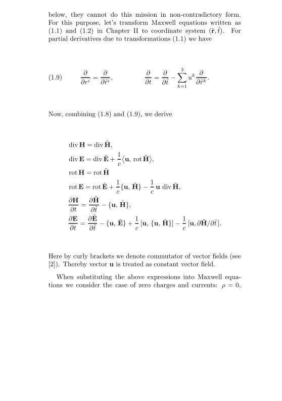
below, they cannot do this mission in non-contradictory form.For this purpose, let’s transform Maxwell equations written as(1.1) and (1.2) in Chapter II to coordinate system (r, t). Forpartial derivatives due to transformations (1.1) we have

∂

∂ri=

∂

∂ri,

∂

∂t=

∂

∂t−

3∑k=1

uk ∂

∂rk.(1.9)

Now, combining (1.8) and (1.9), we derive

div H = div H,

div E = div E +1c

⟨u, rot H

⟩,

rotH = rot H

rotE = rot E +1cu, H − 1

cu div H,

∂H∂t

=∂H∂t

− u, H,∂E∂t

=∂E∂t

− u, E+1c

[u, u, H]− 1c

[u, ∂H/∂t ].

Here by curly brackets we denote commutator of vector fields (see[2]). Thereby vector u is treated as constant vector field.

When substituting the above expressions into Maxwell equa-tions we consider the case of zero charges and currents: ρ = 0,

j = 0. This yields the following equations:

div H = 0,

div E = −1c

⟨u, rot H

⟩,

rot H =1c

∂E∂t

− 1cu, E+

+1c2

[u, u, H]− 1c2

[u, ∂H/∂t ],

rot E = −1c

∂H∂t

.

Only two of the above four equations coincide with originalMaxwell equations. Other two equations contain the entriesof vector u that cannot be eliminated.

This circumstance that we have found is very important. In theend of XIX-th century it made a dilemma for physicists. The wayhow this dilemma was resolved had determined in most furtherdevelopment of physics in XX-th century. Indeed, one had tomake the following crucial choice:

(1) to admit that Maxwell equations are not invariant withrespect to Galileo transformations, hence they require theexistence of some marked inertial coordinate system wherethey have standard form given in the very beginning ofChapter II;

(2) or to assume that formulas (1.1) are not correct, hencerelativity principle claiming equivalence of all inertial co-ordinate systems is realized in some different way.

First Choice had lead to ether theory. According to this theory,marked inertial coordinate system is bound to some hypotheticalmatter, which was called ether. This matter has no mass, no

color, and no smell. It fills the whole space and does not revealitself otherwise, but as a carrier of electromagnetic interaction.Specified properties of ether look quite unusual, this makes ethertheory too artificial (not natural). As a compromise this theorywas admitted for a while, but later was refuted by experiments ofMichaelson and Morley, who tried to measure the Earth velocityrelative to ether (ether wind).

Second choice is more crucial. Indeed, refusing formulas (1.1),we refuse classical mechanics of Newton in whole. Neverthelessthe development of science went through this second choice.

§ 2. Lorentz transformations.

Having refused formulas (1.1), one should replace them bysomething else. This was done by Lorentz. Following Lorentz,now we replace Galileo transformations (1.1) by general lineartransformations relating (r, t) and (r, t):

c t = S00 c t+

3∑k=1

S0k r

k, ri = Si0 c t+

3∑k=1

Sik r

k.(2.1)

In (2.1) we introduced c as a factor for time variables t and t inorder to equalize measure units. Upon introducing this factor allcomponents of matrix S appear to be purely numeric quantitiesthat do not require measure units at all. It is convenient to denotec t by r0 and treat this quantity as additional (fourth) componentof radius-vector:

(2.2) r0 = ct.

Then two relationships (2.1) can be united into one relationship:

(2.3) ri =3∑

k=0

Sik r

k.

In order to have invertible transformation (2.3) one should assumethat detS 6= 0. Let T = S−1. Then inverse transformation for(2.3) is written as follows:

(2.4) ri =3∑

k=0

T ik r

k.

By their structure transformation (2.3) and (2.4) coincide withtransformations of coordinates of four-dimensional vector underthe change of base. Soon we shall see that such interpretationappears to be very fruitful.

Now the problem of deriving Lorentz transformations can beformulated as problem of finding components of matrix S in (2.3).The only condition we should satisfy thereby is the invarianceof Maxwell equations with respect to transformations (2.3) uponcompleting them with transformations for ρ, j, E and H.

For the beginning let’s consider the case with no currents andcharges, i. e. the case ρ = 0, j = 0. Instead of Maxwell equationslet’s study their differential consequences written in form of theequations (4.6) in Chapter II:

E = 0, H = 0.(2.5)

Invariance of (2.5) under the transformations (2.3) and (2.4) isnecessary (but possibly not sufficient) condition for invariance ofMaxwell equations from which the equations (2.5) were derived.

Further we need the following formula for d’Alambert operatorused in the above equations (2.5):

(2.6) =3∑

i=0

3∑j=0

gij ∂

∂ri

∂

∂rj.

Here by gij we denote components of matrix

(2.7) gij = gij =

1 0 0 00 −1 0 00 0 −1 00 0 0 −1

.

It is easy to see that inverse matrix gij for (2.7) has the samecomponents, i. e. gij = gij .

From (2.3) and (2.4) we derive the following transformationrules for first order differential operators:

∂

∂ri=

3∑k=0

T ki

∂

∂rk,

∂

∂ri=

3∑k=0

Ski

∂

∂rk.(2.8)

Substituting (2.8) into formula (2.6), we get

=3∑

p=0

3∑q=0

gpq ∂

∂rp

∂

∂rq,

where matrices gij and gpq are related by formula

(2.9) gpq =3∑

i=0

3∑j=0

T pi T

qj g

ij .

In terms of inverse matrices gpq and gpq this relationship (2.9) canbe rewritten as follows:

(2.10) gij =3∑

p=0

3∑q=0

T pi T

qj gpq.

Theorem 2.1. For any choice of operator coefficients α1, α2,β1, and β2 in formulas (1.6) the invariance of the form of equations(2.5) under the transformations (2.3) and (2.4) is equivalent toproportionality of matrices g and g, i. e.

(2.11) gij = λ gij .

Numeric factor λ in formula (2.11) is usually chosen to be equalto unity: λ = 1. In this case from (2.10) and (2.11) we derive

(2.12) gij =3∑

p=0

3∑q=0

T pi T

qj gpq.

In matrix form this relationship (2.12) looks like

(2.13) T t g T = g.

Here g is a matrix of the form (2.7), while by T t in (2.13) wedenote transposed matrix T .

Definition 2.1. Matrix T satisfying the relationship (2.13) iscalled Lorentzian matrix.

It is easy to check up that the set of Lorentzian matrices forma group. This group is usually denoted by O(1, 3). It is calledmatrix Lorentz group.

From the relationship (2.13) for Lorentzian matrix we derivethe equality (det T )2 = 1. Hence detT = ±1. Lorentzian matrices

with unit determinant form the group SO(1, 3), it is called specialmatrix Lorentz group.

If i = j = 0, from (2.12) we obtain the following formularelating components of Lorentzian matrix T :

(2.14) (T 00 )2 − (T 1

0 )2 − (T 20 )2 − (T 3

0 )2 = 1.

Inequality |T 00 | > 1 is immediate consequence of the relationship

(2.14). Hence T 00 > 1 or T 0

0 6 −1. Lorentzian matrix with T 00 > 1

is called orthochronous. The set of orthochronous Lorentzian ma-trices form orthochronous matrix Lorentz group O+(1, 3). Intersec-tion SO+(1, 3) = SO(1, 3)∩O+(1, 3) is called special orthochronousmatrix Lorentz group.

Exercise 2.1. Prove theorem 2.1 under the assumption thattransformation (1.6) given by operator coefficients α1, α2, β1, andβ2 is invertible.

§ 3. Minkowsky space.

In previous section we have found that each Lorentzian matrixfrom group O(1, 3) determines some transformation (2.1) pre-serving the form the equations (2.5). In deriving this fact weintroduced notations (2.2) and united space and time into onefour-dimensional “space-time”. Let’s denote it by M . Four-dimensional space M is basic object in special theory of relativity.Its points are called events. The space of events is equipped withquadratic form g with signature (1, 3). This quadratic form iscalled Minkowsky metric. Thereby inertial coordinate systems areinterpreted as Cartesian coordinates for which Minkowsky metrichas canonical form (2.7).

Equivalence principle. All physical laws in any two inertialcoordinate systems are written in the same form.

Let’s choose some inertial coordinate system. This choicedetermines separation of event space M into geometric space V

(space of points) and time axis T :

(3.1) M = T ⊕ V.

Matrix of Minkowsky metric in chosen coordinate system hascanonic form (2.7). Therefore geometric space V is orthogonal totime axis T with respect to Minkowsky metric g. Restriction ofthis metric to V is negative quadratic form. Changing its sign,we get positive quadratic form. This is standard Euclidean scalarproduct in V .

Now let’s consider another inertial coordinate system. Like(3.1), it determines second expansion of M into space and time:

(3.2) M = T ⊕ V .

In general time axes T and T in expansions (3.1) and (3.2) donot coincide. Indeed, bases of these two coordinate systems arerelated to each other by formula

(3.3) ei =3∑

j=0

Sji ej ,

where S is Lorentzian matrix from (2.3). For base vector e0

directed along time axis T from (3.3) we derive

(3.4) e0 = S00 e0 + S1

0 e1 + S20 e2 + S3

0 e3.

In general components S10 , S2

0 , and S30 in Lorentz matrix S are

nonzero. Therefore vectors e0 and e0 are non-collinear. HenceT 6= T .

Non-coincidence of time axes T 6= T for two inertial coordinatesystems leads to non-coincidence of geometric spaces: V 6= V .This fact lead to quite radical conclusion when we interpretit physically: observers in two such inertial systems observe two

different three-dimensional geometric spaces and have two differenttime ticks. However, in our everyday life this difference is verysmall and never reveals.

Let’s calculate how big is the difference in the rate of time ticksfor two inertial coordinate systems. From (2.4) we get

(3.5) t = T 00 t+

3∑k=1

T 0k

crk.

Let t → +∞. If Lorentzian matrix T is orthochronous, thenT 0

0 > 0 and t → +∞. If matrix T is not orthochronous, thent → +∞ we get t → −∞. Transformations (2.4) with non-orthochronous matrices T invert the direction of time exchangingthe future and the past. It would be very intriguing to have sucha feature in theory. However, presently in constructing theory ofrelativity one uses more realistic approach. So we shall assumethat two physically real inertial coordinate systems can be relatedonly by orthochronous Lorentz matrices from O+(1, 3).

Restriction of the set of admissible Lorentz matrices fromO(1, 3) to O+(1, 3) is due to the presence of additional structurein the space of events. It is called polarization. Let’s choose somephysical inertial coordinate system. Minkowsky metric in suchsystem is given by matrix of canonical form (2.7). Let’s calculatescalar square of four-dimensional vector x in Minkowsky metric:

(3.6) g(x, x) = (x0)2 − (x1)2 − (x2)2 − (x3)2.

By value of their scalar square g(x, x) in Minkowsky metric g

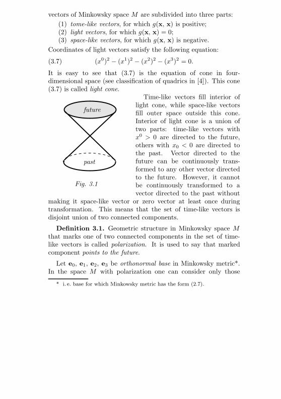
vectors of Minkowsky space M are subdivided into three parts:(1) tome-like vectors, for which g(x, x) is positive;(2) light vectors, for which g(x, x) = 0;(3) space-like vectors, for which g(x, x) is negative.

Coordinates of light vectors satisfy the following equation:

(3.7) (x0)2 − (x1)2 − (x2)2 − (x3)2 = 0.

It is easy to see that (3.7) is the equation of cone in four-dimensional space (see classification of quadrics in [4]). This cone(3.7) is called light cone.

Time-like vectors fill interior oflight cone, while space-like vectorsfill outer space outside this cone.Interior of light cone is a union of

Fig. 3.1

past

future

two parts: time-like vectors withx0 > 0 are directed to the future,others with x0 < 0 are directed tothe past. Vector directed to thefuture can be continuously trans-formed to any other vector directedto the future. However, it cannotbe continuously transformed to avector directed to the past without

making it space-like vector or zero vector at least once duringtransformation. This means that the set of time-like vectors isdisjoint union of two connected components.

Definition 3.1. Geometric structure in Minkowsky space Mthat marks one of two connected components in the set of time-like vectors is called polarization. It is used to say that markedcomponent points to the future.

Let e0, e1, e2, e3 be orthonormal base in Minkowsky metric*.In the space M with polarization one can consider only those

* i. e. base for which Minkowsky metric has the form (2.7).

such bases for which unit vector of time axis e0 is directed to thefuture. Then transition from one of such bases to another wouldbe given by orthochronous matrix from group O+(1, 3).

Definition 3.2. Four-dimensional affine space M equippedwith metric g of signature (1, 3) and equipped with orientation**and polarization is called Minkowsky space.

According to special theory of relativity Minkowsky space,which is equipped with orientation and polarization, is propermathematical model for the space of real physical events. Nowwe can give strict mathematical definition of inertial coordinatesystem.

Definition 3.3. Orthonormal right inertial coordinate systemis orthonormal right coordinate system in Minkowsky space withtime base vector directed to the future.

It is easy to verify that any two inertial coordinate systems asdefined above are related to each other by Lorentz transforma-tion with matrix S from orthochronous Lorentz group SO+(1, 3).Let’s choose one of such coordinate systems and consider relatedexpansion (3.1). It is clear that e0 ∈ T , while linear span ofspatial vectors e1, e2, e3 defines subspace V . Taking orthonormalbase e1, e2, e3 for the standard of right bases in V , we equipthis three-dimensional space with orientation. This is concor-dance with the fact that geometric space that we observe in oureveryday life possesses orientation distinguishing left and right.

Exercise 3.1. By analogy with definition 3.3 formulate thedefinition of skew-angular inertial coordinate system.

§ 4. Kinematics of relative motion.

Galileo transformations are used in mechanics for describingphysical processes as they are seen by two observers representing

** remember that orientation is geometric structure distinguishing left andright bases (see [4]).

two inertial coordinate systems. Lorentz transformations, whichwe have derived from the condition of invariance of electrodynam-ical equations (2.5), are designed for the same purpose. However,this is not immediately clear when looking at formulas (2.3) and(2.4). Therefore we shall bring these formulas to the form moreconvenient for studying their physical nature.

Let’s fix two inertial coordinate systems related by Lorentztransformation (2.1). First one is related with orthonormal basee0, e1, e2, e3 in Minkowsky space and with the expansion (3.1).Second is related with the base e0, e1, e2, e3 and with theexpansion (3.2). If time axes are parallel e0 = e0, then Lorentzmatrix S in (2.3) is reduced to orthogonal matrix O ∈ SO(3)relating two right orthonormal bases e1, e2, e3 and e1, e2, e3. Ithas the following blockwise-diagonal shape:

(4.1) S =

1 0 0 00 O1

1 O12 O1

3

0 O21 O2

2 O23

0 O31 O3

2 O33

.

Thus, in case if T ‖ T two inertial coordinate systems differ onlyin directions of spatial axes. They do not move with respect toeach other.

Now let’s consider the case T ∦ T . Hence e0 6= e0. Let H belinear span of vectors e0 and e0. Denote by W intersection ofsubspaces V and V from (3.1) and (3.2):

H = Span(e0, e0), W = V ∩ V .(4.2)

Lemma 4.1. Two-dimensional subspacesH andW in (4.2) areperpendicular to each other in Minkowsky metric g. Their inter-section is zero: H ∩W = 0, while direct sum of these subspacescoincides with the whole Minkowsky space: H ⊕W = M .

Proof. Subspace H is two-dimensional since it is linear spanof two non-collinear vectors. Subspaces V and V are three-dimensional and V 6= V . Hence their sum V + V coincides with

M , i. e. dim(V + V ) = 4. Applying theorem on the dimension ofsum and intersection of two subspaces (see [4]), we get

dim(W ) = dim V + dim V − dim(V + V ) = 3 + 3− 4 = 2.

In order to prove orthogonality of H and W we use orthogonal-ity of T and V in the expansion (3.1) and orthogonality of T andV in (3.2). Let y be an arbitrary vector in subspace W . Theny ∈ V . From V ⊥ T we get y ⊥ e0. Analogously from y ∈ V weget y ⊥ e0. Now from orthogonality of y to both vectors e0 ande0 we derive orthogonality of y to their linear span: y ⊥ H . Sincey is arbitrary vector in W , we have W ⊥ H .

Now let’s prove that H ∩W = 0. Let’s consider an arbitraryvector x ∈ H ∩W . From x ∈ H and x ∈ W due to orthogonalityof H and W , which is already proved, we get g(x,x) = 0. Butx ∈ W ⊂ V , while restriction of Minkowsky metric to subspaceV is negative quadratic form of signature (0, 3). Therefore fromg(x,x) = 0 we derive x = 0. Proposition H ∩W = 0 is proved.

From H ∩W = 0 we conclude that sum of subspaces H andW is direct sum and dim(H+W ) = 2+2 = 4. Hence H⊕W = M .Lemma is proved.

Now let’s return back to considering pair of inertial coordinatesystems with bases e0, e1, e2, e3 and e0, e1, e2, e3. There is theexpansion (3.4) for vector e0. Let’s write it as follows:

(4.3) e0 = S00 e0 + v.

Here v = S10 e1 + S2

0 e2 + S30 e3 ∈ V . Since matrix S is or-

thochronous and since e0 6= e0, we have

S00 > 1, v 6= 0.(4.4)

For any real number a > 1 there exists a number α > 0 such thata = cosh(α). Let’s apply this observation to S0

0 in (4.3):

(4.5) S00 = cosh(α).

From (4.3), from (4.5), and from orthogonality of vectors e0 andv in Minkowsky metric we obtain

1 = g(e0, e0) = (S00)2 g(e0, e0) + g(v,v) = cosh2(α)− |v|2.

Using this equality we can find Euclidean length of vector v inthree-dimensional subspace V :

(4.6) |v| = sinh(α), where α > 0.

Let’s replace vector v by vector of unit length h1 = v/|v| andrewrite the relationship (4.3) as follows:

(4.7) e0 = cosh(α) e0 + sinh(α)h1.

Due to (4.7) vector h1 is linear combination of vectors e0 and e0,hence h1 ∈ H . But h1 ∈ V as well. Therefore h1 ∈ V ∩H . Vectorse0 and h1 are perpendicular to each other, they form orthonormalbase in two-dimensional subspace H :

g(e0, e0) = 1, g(h1,h1) = −1.(4.8)

From (4.8) we conclude that restriction of Minkowsky metric tosubspace H is metric with signature (1, 1).

Now we need another vector from subspace H . Let’s determineit by the following relationship:

(4.9) h1 = sinh(α) e0 + cosh(α)h1.

It is easy to check that vectors e0 and h1 form another orthonor-mal base in subspace H . Transition matrix relating these twobases has the following form:

(4.10) SL =

(cosh(α) sinh(α)

sinh(α) cosh(α)

).

Matrix (4.10) is called the matrix of Lorentzian rotation.There is four-dimensional version of matrix (4.10). Indeed,

vector h1 ∈ V is perpendicular to subspace W ⊂ V . Therefore wehave the expansion of subspace V as a direct sum:

V = Span(h1)⊕W.

Let’s choose two vectors h2 and h3 forming orthonormal basein subspace W and complementing h1 up to an orthonormalright base in V . Then four vectors e0, h1, h2 h3 constituteorthonormal right base in M with time vector e0 directed tothe future. Transition matrix relating this base with the basee0, h1, h2 h3 has the following blockwise-diagonal form:

(4.11) SL =

cosh(α) sinh(α) 0 0

sinh(α) cosh(α) 0 0

0 0 1 0

0 0 0 1

.

Transition from base e0, e1, e2 e3 to base e0, h1, h2 h3 is givenby a matrix of the form (4.1). This is because their time vectorsdo coincide. In a similar way transition from base e0, h1, h2 h3

to base e0, e1, e2 e3 is given by a matrix of the same form(4.1). Ultimate change of base e0, e1, e2 e3 for another basee0, e1, e2 e3 then can be done in three steps.

Theorem 4.1. Each Lorentzian matrix S ∈ SO+(1, 3) is aproduct of three matrices S = S1 SL S2, one of which SL is amatrix of Lorentzian rotation (4.11), while two others S1 and S2

are matrices of the form (4.1).

In order to clarify physical meaning of Lorentz transformationslet’s first consider transformations with matrix S of the form(4.11). Let ct = r0, r1, r2, r3 be coordinates of some vector

r ∈M in the base e0, h1, h2, h3. By ct = r0, r1, r2, r3 we denotecoordinates of the same vector in the base e0, h1, h2 h3. Formatrix S of the form (4.11) formula (2.3) leads to relationships

(4.12)

t = cosh(α) t+sinh(α)

cr1,

r1 = sinh(α) c t+ cosh(α) r1,

r2 = r2,

r3 = r3.

Let r1, r2, r3 be coordinates of radius-vector of some point Awhich is at rest in inertial coordinate system with base e1, e2, e3.Then r1, r2, r3 are constants, they do not depend on time t inthis coordinate system. Upon calculating coordinates of this pointA in other inertial coordinate system by means of formulas (4.12)its first coordinate r1 appears to be a function of parameter t.We use first relationship (4.12) in order to express parameter tthrough time variable t in second coordinate system:

(4.13) t =t

cosh(α)− tanh(α)

cr1.

Substituting (4.13) into other three formulas (4.12), we get

(4.14)

r1 = r1(t) = c tanh(α) t+ const,

r2 = r2(t) = const,

r3 = r3(t) = const .

From (4.14) we see that in second coordinate system our point Ais moving with constant velocity u = c tanh(α) in the direction offirst coordinate axis.

In contrast to parameter α in matrix (4.11), parameter uhas transparent physical interpretation as magnitude of relative

velocity of one coordinate system with respect to another. Let’sexpress components of matrix (4.11) through u:

cosh(α) =1√

1− u2

c2

, sinh(α) =u

c

1√1− u2

c2

.

Let’s substitute these formulas into (4.12). As a result we get

t =t+

u

c2r1√

1− u2

c2

, r1 =ut+ r1√1− u2

c2

,

(4.15)

r2 = r2, r3 = r3.

Denote for a while by r and r the following two three-dimensional vectors in subspaces V and V :

(4.16)r = r1 h1 + r2 h2 + r3 h3,

r = r1 h1 + r2 h2 + r3 h3.

Then we define linear map θ : V → V determined by its actionupon base vectors h1, h2, and h3:

θ(h1) = h1, θ(h2) = h2, θ(h3) = h3.

This map θ is orientation preserving isometry, since it maps rightorthonormal base of subspace V to right orthonormal base insubspace V . Using above notations (4.16) and the map θ, we can

write formulas (4.15) in vectorial form:

(4.17)

t =t+

⟨θu, r

⟩c2√

1− |u|2c2

,

θr =θu t+

⟨θu, r

⟩|u|2 θu√

1− |u|2c2

+ r−⟨θu, r

⟩|u|2 θu.

Here u = uh1 is vector of relative velocity of second coordinatesystem with respect to first one. Formulas (4.17) are irrespectiveto the choice of bases in subspaces V and V . Therefore they areapplicable to Lorentz transformations with special matrix of theform (4.11) and to arbitrary Lorentz transformations with matrixS = S1 SL S2 (see theorem 4.1).

Very often the sign of map θ realizing isomorphism of subspacesV and V in formulas (4.17) is omitted:

(4.18)

t =t+

⟨u, r

⟩c2√

1− |u|2c2

,

r =u t+

⟨u, r

⟩|u|2 u√

1− |u|2c2

+ r−⟨u, r

⟩|u|2 u.

Formulas (4.18) represent “conditionally three-dimensional” un-derstanding of Lorentz transformations when vectors r and r

treated as vectors of the same three-dimensional Euclidean space,while t and t are treated as scalar parameters. However, accord-ing to modern paradigm four-dimensional Minkowsky space is realphysical entity, not purely mathematical abstraction convenientfor shortening formulas (compare (2.3) and (4.17)).

When writing formulas (4.17) and (4.18) in components weshould expand vectors r and u in the base of one coordinate sys-tem, while vector r is expanded in the base of another coordinatesystem. Thereby the difference in the shape of these two formulascompletely disappears.

Exercise 4.1. Using expansions (4.16) for vectors r and r, de-rive the following formulas:

r1 =

⟨θu, r

⟩|u| , r2 h2 + r3 h3 = r−

⟨θu, r

⟩|u|2 θu.

Combining these formulas with (4.15), derive formulas (4.17).

§ 5. Relativistic law of velocity addition.

Classical law of velocity addition was first consequence that weobtained from Galileo transformations:

(5.1) v = v + u,

see formulas (1.2). Replacing Galileo transformations by Lorentztransformations, now we should derive new relativistic law ofvelocity addition.

Suppose that vector-function r(t) describes the motion of apoint A in inertial coordinate system (r, t) and suppose that thiscoordinate system moves with velocity u with respect to otherinertial coordinate system (r, t). For passing to coordinate system(r, t) we use Lorentz transformation given by formulas (4.18). As

a result we get two functions

(5.2)

t(t) =t+

⟨u, r(t)

⟩c2√

1− |u|2c2

,

r(t) =u t+

⟨u, r(t)

⟩|u|2 u√

1− |u|2c2

+ r(t)−⟨u, r(t)

⟩|u|2 u.

Let’s calculate first derivatives of functions (5.2):

(5.3a)dt

dt=

1 +

⟨u, v

⟩c2√

1− |u|2c2

,

(5.3b)drdt

=u +

⟨u, v

⟩|u|2 u√

1− |u|2c2

+ v −⟨u, v

⟩|u|2 u.

By v we denote the velocity of the point A in coordinates (r, t):

v = ˙r(t) =drdt.

In a similar way by v we denote the velocity of this point in othercoordinates (r, t). To calculate v we divide derivatives:

(5.4) v =drdt

= r(t) =(drdt

)/(dt

dt

).

Substituting (5.3a) and (5.3b) into (5.4), we get formula

(5.5) v =u +

⟨u, v

⟩|u|2 u

1 +

⟨u, v

⟩c2

+v −

⟨u, v

⟩|u|2 u

1 +

⟨u, v

⟩c2

√1− |u|2

c2.

Formula (5.5) is relativistic law of velocity addition. It is machmore complicated than classical law given by formula (5.1). How-ever, in the limit of small velocities |u| c formula (5.5) reducesto formula (5.1).

Exercise 5.1. Derive relativistic law of velocity addition fromformula (4.17). Explain why resulting formula differs from (5.5).

§ 6. World lines and private time.

Motion of point-size material object in arbitrary inertial coor-dinate system (r, t) is described by vector-function r(t), where tis time variable and r is radius-vector of point. Four-dimensionalradius-vector of this material point has the following components:

(6.1) r0(t) = ct, r1(t), r2(t), r3(t).

Vector-function with components (6.1) determines parametric linein Minkowsky space M , this line is called world line of materialpoint. Once world line is given, motion of material point isdescribed completely. Let’s differentiate four-dimensional radius-vector (6.1) with respect to parameter t. As a result we getfour-dimensional vector tangent to world line:

(6.2) K = (c, r1, r2, r3) = (c, v1, v2, v3).

Last three components of this vector form velocity vector ofmaterial point. Velocity of most material objects is not greaterthan light velocity: |v| < c. When applied to vector K in (6.2)this means that tangent-vector of world line is time-like vector:

(6.3) g(K,K) = c2 − |v|2 > 0.

Definition 6.1. Smooth curve in Minkowsky space is calledtime-like curve if tangent-vector of this curve is time-like vectorat each its point.

World lines for most material objects are time-like curves.Exception are world lines of photons (light particles) and worldlines of other elementary particles with zero mass. For them|v| = c, hence we get g(K,K) = 0.

World line have no singular points. Indeed, even if g(K,K) =0, tangent vector K in (6.2) is nonzero since K0 = c 6= 0.

Let’s consider world line of material point of nonzero mass.

For this line we have the condition (6.3) fulfilled, hence we canintroduce natural parameter on this line:

(6.4) s(t) =

t∫t0

√g(K,K) dt.

Integral (6.4) yields invariant parameter for world lines. For anytwo points A and B on a given world line the quantity s(B)−s(A)does not depend on inertial coordinate system used for calculatingintegral (6.4). This quantity is called interval length of the arcAB on world line.

Theorem 6.1. Straight line segment connecting end points ofan arc on smooth time-like curve is a segment of time-like straightline. Its interval length is greater than interval length of corre-sponding arc.

Let A and B be two successive events in the “life” of materialpoint of nonzero mass. The answer to the question what time in-terval separates these two events depend on the choice of inertialcoordinate system from which we observe the “life” of this ma-terial point. So this answer is relative (not invariant). However,there is invariant quantity characterizing time distance betweentwo events on world line:

(6.5) τ =s(B)− s(A)

c.

This quantity τ in formula (6.5) is called interval of private timeon world line.

Concept of private time determine microlocal concept of timein theory of relativity. According to this concept each materialpoint lives according to its own watch, and watches of differentmaterial points are synchronized only in very rough way: theycount time from the past to the future. This rough synchroniza-tion is determined by polarization in Minkowsky space. Exact

synchronization of watches is possible only when material pointscome to immediate touch with each other, i. e. when their worldlines intersect. However, even after such exact synchronizationin the point of next meeting watches of tho material points willshow different times. This difference is due to different ”lifepaths” between two meetings.

Concept of private time is illustrated by so-called twins prob-lem, well-known from science fiction. Suppose that one of twinsgoes to far-away travel in interstellar spacecraft, while his brotherstays on the Earth. Which of them will be older when they meeteach other on the Earth in the end of space voyage.

The answer is: that one who stayed on the Earth will be older.World lines of twins intersect twice. Both intersections occur onthe Earth, one before travel and other after travel. Its known thatCoordinate system associated with the Earth can be taken forinertial coordinate system with high degree of accuracy (indeed,acceleration due to rotation of the Earth around its axis and dueto orbital rotation around the Sun is not sensible in our everydaylife). Therefore world line of twin stayed on the Earth is straightline. World line of twin in spacecraft is curved. In the beginningof travel he accelerates reaching substantial velocity comparablewith light velocity in the middle of the path. Then he experiencesbackward acceleration in order to brake before reaching targetpoint of his travel. Then he accelerates and brakes again in hisback way to the Earth. According to theorem 6.1 interval lengthof curved world line connecting two events is shorter than intervallength of straight world line connecting the same two events.Hence twin stayed on the Earth will be older.

Exercise 6.1. Remember proof of the fact that the length ofcurved line connecting two points A and B in Euclidean space isgreater than the length of straight line segment AB. By analogyto this proof find the proof for theorem 6.1.

§ 7. Dynamics of material point.

Motion of material point in theory of relativity is described byits world line in Minkowsky space. Let’s choose natural parameteron world line and consider four-dimensional tangent vector

(7.1) u(s) =dr(s)ds

,

where r(s) is four-dimensional radius vector of events on worldline. Vector u is (7.1) is called vector of 4-velocity. It is time-likevector and it is unit vector in Minkowsky metric: g(u,u) = 1.Upon choosing some inertial coordinate system we can writecomponents of 4-velocity vector explicitly:

(7.2) u =1√

c2 − |v|2

∥∥∥∥∥∥∥cv1

v2

v3

∥∥∥∥∥∥∥ .Here v1, v2, v3 are components of three-dimensional velocityvector v. Note that components u0, u1, u2, u3 of 4-velocity vectorare absolute numbers (without measure unit). It is easy to seefrom (7.2). Upon multiplying u by scalar mc with the measureunit of momentum we get vector of 4-momentum

(7.3) p =m√

1− |v|2c2

∥∥∥∥∥∥∥cv1

v2

v3

∥∥∥∥∥∥∥for material point with mass m. Vector p plays important rolein physics since there is fundamental law of nature: the law ofconservation of 4-momentum.

Momentum conservation law. Vector of 4-momentum ofmaterial point which do not experience external action remainsunchanged.

According to the law just stated, for particle that do notexperience external action we have p = const. Hence u = const.Integrating the equation (7.1), for r(s) we derive

r(s) = r0 + u s.

Conclusion: in the absence of external action material point movesuniformly along straight line.

External actions causing change of 4-momentum of materialpoint are subdivided into two categories:

(1) continuous;(2) discrete.

Continuous actions are applied to material particle by externalfields. They cause world line to bend making it curved line. Inthis case p 6= const. Derivative of 4-momentum with respect tonatural parameter s is called vector of 4-force:

(7.4)dpds

= F(s).

Vector of 4-force in (7.4) is quantitative characteristic of theaction of external fields upon material particle. It is determinedby parameters of particle itself and by parameters of externalfields at current position of particle as well. We know thatvector of 4-velocity u is unit vector, therefore g(p,p) = m2 c2.Differentiating this relationship with respect to s and taking intoaccount that components of matrix (2.7) are constant, we find

(7.5) g(u,F) = 0.

The relationship (7.5) means that vector of 4-force is perpendicu-lar to vector of 4-velocity in Minkowsky metric, i. e. force vectoris perpendicular to world line of particle.

Choosing some inertial coordinate system, we can replace nat-ural parameter s in (7.5) by time variable t of this coordinatesystem. Then, taking into account (7.3), from (7.4) we derive

(7.6)dpi

dt=√c2 − |v|2 F i, where i = 1, 2, 3.

Now, if we denote by f three-dimensional vector with compo-nents f i =

√c2 − |v|2 F i, then for three-dimensional vector of

momentum from (7.6) we obtain differential equation

(7.7)dpdt

= f .

The equation (7.7) is treated as relativistic analog of Newton’ssecond law. Instead of classical formula p = mv relating momen-tum and velocity vectors here we have the following relationship:

(7.8) p =mv√

1− |v|2c2

.

In order to write (7.8) in classical form we introduce the quantity

(7.9) mv =m√

1− |v|2c2

.

Constant m is called mass at rest, while mv in (7.8) is calleddynamic mass of moving particle. Now p = mv v, and Newton’ssecond law is written as follows:

(7.10) (mv v)′t = f .

Formulas (7.9) and (7.10) are the very ones which are in mindwhen one says that mass in theory of relativity depends on

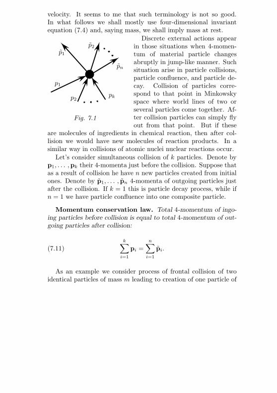
velocity. It seems to me that such terminology is not so good.In what follows we shall mostly use four-dimensional invariantequation (7.4) and, saying mass, we shall imply mass at rest.

Discrete external actions appearin those situations when 4-momen-tum of material particle changesabruptly in jump-like manner. Suchsituation arise in particle collisions,particle confluence, and particle de-cay. Collision of particles corre-

Fig. 7.1

p2pk

p1

pn

p1

p2

spond to that point in Minkowskyspace where world lines of two orseveral particles come together. Af-ter collision particles can simply flyout from that point. But if these

are molecules of ingredients in chemical reaction, then after col-lision we would have new molecules of reaction products. In asimilar way in collisions of atomic nuclei nuclear reactions occur.

Let’s consider simultaneous collision of k particles. Denote byp1, . . . ,pk their 4-momenta just before the collision. Suppose thatas a result of collision he have n new particles created from initialones. Denote by p1, . . . , pn 4-momenta of outgoing particles justafter the collision. If k = 1 this is particle decay process, while ifn = 1 we have particle confluence into one composite particle.

Momentum conservation law. Total 4-momentum of ingo-ing particles before collision is equal to total 4-momentum of out-going particles after collision:

(7.11)k∑

i=1

pi =n∑

i=1

pi.

As an example we consider process of frontal collision of twoidentical particles of mass m leading to creation of one particle of

mass M . Suppose that velocities of initial particles are equal bymagnitude but opposite to each other:

p1 =m√

1− |v|2c2

∥∥∥∥∥∥∥cv1

v2

v3

∥∥∥∥∥∥∥ , p2 =m√

1− |v|2c2

∥∥∥∥∥∥∥c−v1

−v2

−v3

∥∥∥∥∥∥∥ .For 4-momentum of resulting particle we have

p1 =M√

1− |w|2c2

∥∥∥∥∥∥∥cw1

w2

w3

∥∥∥∥∥∥∥ .Applying momentum conservation law (7.11) to this situation, weget w = 0 and additionally we obtain

(7.12) M =2m√

1− |v|2c2

.

From (7.12) we see that mass at rest of resulting compositeparticle is greater than sum of rest masses of its components:M > m+m. Conclusion: the low of mass conservation is fulfilledapproximately only in the limit of small velocities |v| c.

Let’s multiply zeroth component of 4-momentum of materialparticle by c. Resulting quantity has the measure unit of energy.Let’s denote this quantity by E:

(7.13) E =mc2√

1− |v|2c2

.

The quantity (7.13) is called kinetic energy of moving particle.Writing relationship (7.11) for zeroth components of collidingparticles, we get energy conservation law:

(7.14)k∑

i=1

Ei =n∑

i=1

Ei.

Thus, 4-momentum conservation law for collision includes bothenergy conservation law (7.14) and the law of conservation forthree-dimensional momentum.

Note that for zero velocity v = 0 the above quantity (7.13)does not vanish, but takes nonzero value

(7.15) E = mc2.

This quantity is known as rest energy of material particle. For-mula (7.15) is well-known. It reflects very important fact absentin classical physics: the ability of energy to mass and mass toenergy conversion. In practice conversion of energy to mass isrealized in particle confluence (see M > m+m in formula (7.12)).Converse phenomenon of particle decay yields mass defect (massdecrease). Lost mass is realized in additional amount of kineticenergy of outgoing particles. Total conversion of mass to en-ergy is also possible. This happens in process of annihilation,when elementary particle meets corresponding antiparticle. Largeamount of energy released in annihilation is scattered in form ofshort-wave electromagnetic radiation.

§ 8. Four-dimensional form of Maxwell equations.

Starting from electromagnetic equations E = 0 and H = 0in previous sections we have constructed and described Lorentztransformations preserving form of these equations. We also havegiven geometric and physical interpretation of Lorentz transfor-mations and even have described dynamics of material points on

the base of new relativistic notion of space and time. Now timehas come to remember that equations E = 0 and H = 0are not primary equations of electrodynamics, they were derivedfrom Maxwell equations. To have complete picture we should weshould write Maxwell equations in four-dimensional form. Let’sbegin with second pair of these equations containing charges andcurrents (see equations (1.2) in Chapter II. Let’s modify them:

1c

∂E∂t

− rotH = −4πc

j, − div E = −4πρ.

Then rewrite these equations in components using Levi-Civitasymbol for to express rotor (see [3]):

(8.1)

∂Ep

∂r0−

3∑q=1

3∑k=1

εpqk∂Hk

∂rq= −4π

cjp,

−3∑

q=1

∂Eq

∂rq= −4π ρ.

Here we used notation r0 = ct associating time variable withzeroth component of radius-vector in Minkowsky space.

Using Levi-Civita symbol and components of vector H, we canconstruct skew-symmetric 3× 3 matrix with elements

(8.2) F pq = −3∑

k=1

εpqk Hk.

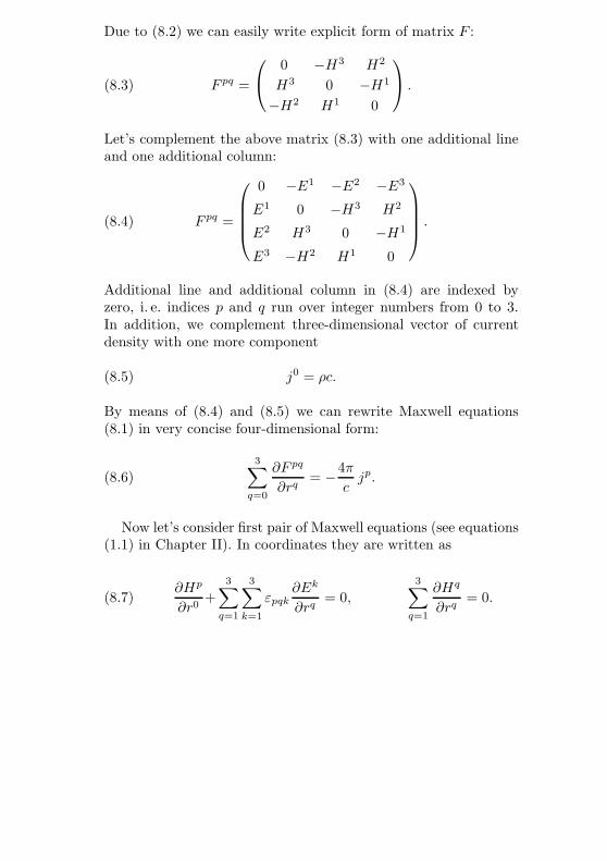
Due to (8.2) we can easily write explicit form of matrix F :

(8.3) F pq =

0 −H3 H2

H3 0 −H1

−H2 H1 0

.

Let’s complement the above matrix (8.3) with one additional lineand one additional column:

(8.4) F pq =

0 −E1 −E2 −E3

E1 0 −H3 H2

E2 H3 0 −H1

E3 −H2 H1 0

.

Additional line and additional column in (8.4) are indexed byzero, i. e. indices p and q run over integer numbers from 0 to 3.In addition, we complement three-dimensional vector of currentdensity with one more component

(8.5) j0 = ρc.

By means of (8.4) and (8.5) we can rewrite Maxwell equations(8.1) in very concise four-dimensional form:

(8.6)3∑

q=0

∂F pq

∂rq= −4π

cjp.

Now let’s consider first pair of Maxwell equations (see equations(1.1) in Chapter II). In coordinates they are written as

∂Hp

∂r0+

3∑q=1

3∑k=1

εpqk∂Ek

∂rq= 0,

3∑q=1

∂Hq

∂rq= 0.(8.7)

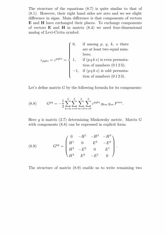
The structure of the equations (8.7) is quite similar to that of(8.1). However, their right hand sides are zero and we see slightdifference in signs. Main difference is that components of vectorsE and H have exchanged their places. To exchange componentsof vectors E and H in matrix (8.4) we need four-dimensionalanalog of Levi-Civita symbol:

εpqks = εpqks =

0, if among p, q, k, s thereare at least two equal num-bers;

1, if (p q k s) is even permuta-tion of numbers (0 1 2 3);

−1, if (p q k s) is odd permuta-tion of numbers (0 1 2 3).

Let’s define matrix G by the following formula for its components:

(8.8) Gpq = −12

3∑k=0

3∑s=0

3∑m=0

3∑n=0

εpqks gkm gsn Fmn.

Here g is matrix (2.7) determining Minkowsky metric. Matrix Gwith components (8.8) can be expressed in explicit form:

(8.9) Gpq =

0 −H1 −H2 −H3

H1 0 E3 −E2

H2 −E3 0 E1

H3 E2 −E1 0

.

The structure of matrix (8.9) enable us to write remaining two

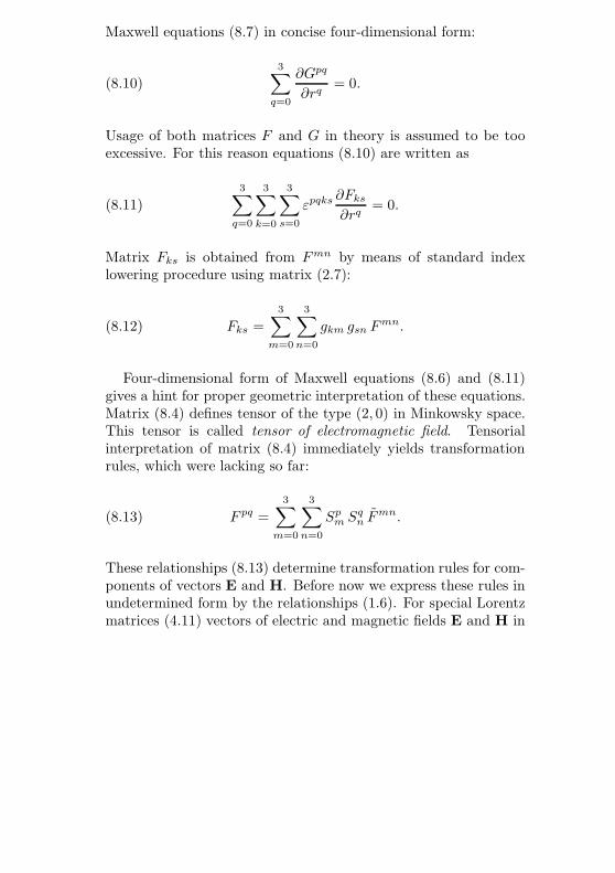
Maxwell equations (8.7) in concise four-dimensional form:

(8.10)3∑

q=0

∂Gpq

∂rq= 0.

Usage of both matrices F and G in theory is assumed to be tooexcessive. For this reason equations (8.10) are written as

(8.11)3∑

q=0

3∑k=0

3∑s=0

εpqks ∂Fks

∂rq= 0.

Matrix Fks is obtained from Fmn by means of standard indexlowering procedure using matrix (2.7):

(8.12) Fks =3∑

m=0

3∑n=0

gkm gsn Fmn.

Four-dimensional form of Maxwell equations (8.6) and (8.11)gives a hint for proper geometric interpretation of these equations.Matrix (8.4) defines tensor of the type (2, 0) in Minkowsky space.This tensor is called tensor of electromagnetic field. Tensorialinterpretation of matrix (8.4) immediately yields transformationrules, which were lacking so far:

(8.13) F pq =3∑

m=0

3∑n=0

Spm Sq

n Fmn.

These relationships (8.13) determine transformation rules for com-ponents of vectors E and H. Before now we express these rules inundetermined form by the relationships (1.6). For special Lorentzmatrices (4.11) vectors of electric and magnetic fields E and H in

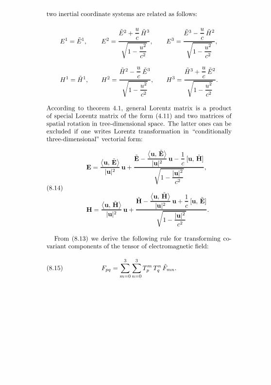
two inertial coordinate systems are related as follows:

E1 = E1, E2 =E2 +

u

cH3√

1− u2

c2

, E3 =E3 − u

cH2√

1− u2

c2

,

H1 = H1, H2 =H2 − u

cE3√

1− u2

c2

, H3 =H3 +

u

cE2√

1− u2

c2

.

According to theorem 4.1, general Lorentz matrix is a productof special Lorentz matrix of the form (4.11) and two matrices ofspatial rotation in tree-dimensional space. The latter ones can beexcluded if one writes Lorentz transformation in “conditionallythree-dimensional” vectorial form:

(8.14)

E =

⟨u, E

⟩|u|2 u +

E−⟨u, E

⟩|u|2 u− 1

c[u, H]√

1− |u|2c2

,

H =

⟨u, H

⟩|u|2 u +

H−⟨u, H

⟩|u|2 u +

1c

[u, E]√1− |u|2

c2

.

From (8.13) we derive the following rule for transforming co-variant components of the tensor of electromagnetic field:

(8.15) Fpq =3∑

m=0

3∑n=0

Tmp T n

q Fmn.

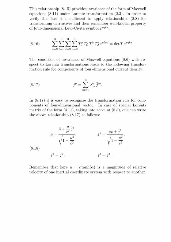
This relationship (8.15) provides invariance of the form of Maxwellequations (8.11) under Lorentz transformation (2.3). In order toverify this fact it is sufficient to apply relationships (2.8) fortransforming derivatives and then remember well-known propertyof four-dimensional Levi-Civita symbol εpqks:

(8.16)3∑

a=0

3∑b=0

3∑c=0

3∑d=0

T pa T

qb T

kc T

sd ε

abcd = detT εpqks.

The condition of invariance of Maxwell equations (8.6) with re-spect to Lorentz transformations leads to the following transfor-mation rule for components of four-dimensional current density:

(8.17) jp =3∑

m=0

Spm jm.

In (8.17) it is easy to recognize the transformation rule for com-ponents of four-dimensional vector. In case of special Lorentzmatrix of the form (4.11), taking into account (8.5), one can writethe above relationship (8.17) as follows:

ρ =ρ+

u

c2j1√

1− u2

c2

, j1 =uρ+ j1√1− u2

c2

,

(8.18)

j2 = j2, j3 = j3.

Remember that here u = c tanh(α) is a magnitude of relativevelocity of one inertial coordinate system with respect to another.

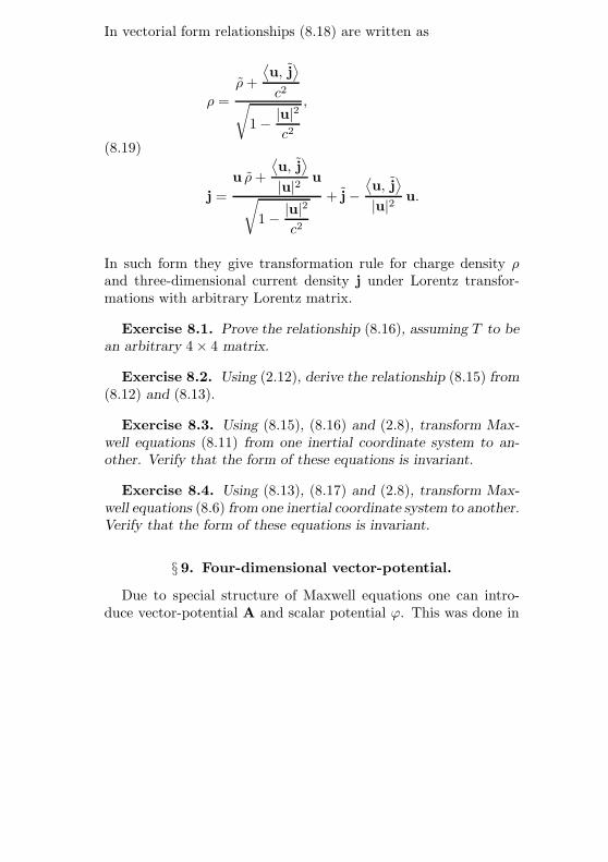
In vectorial form relationships (8.18) are written as

(8.19)

ρ =ρ+

⟨u, j

⟩c2√

1− |u|2c2

,

j =u ρ+

⟨u, j

⟩|u|2 u√

1− |u|2c2

+ j−⟨u, j

⟩|u|2 u.

In such form they give transformation rule for charge density ρand three-dimensional current density j under Lorentz transfor-mations with arbitrary Lorentz matrix.

Exercise 8.1. Prove the relationship (8.16), assuming T to bean arbitrary 4× 4 matrix.

Exercise 8.2. Using (2.12), derive the relationship (8.15) from(8.12) and (8.13).

Exercise 8.3. Using (8.15), (8.16) and (2.8), transform Max-well equations (8.11) from one inertial coordinate system to an-other. Verify that the form of these equations is invariant.

Exercise 8.4. Using (8.13), (8.17) and (2.8), transform Max-well equations (8.6) from one inertial coordinate system to another.Verify that the form of these equations is invariant.

§ 9. Four-dimensional vector-potential.

Due to special structure of Maxwell equations one can intro-duce vector-potential A and scalar potential ϕ. This was done in

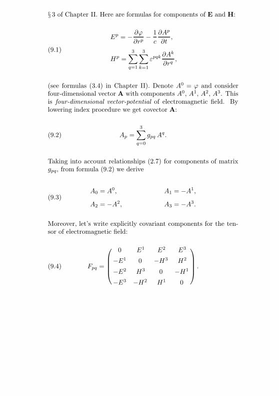
§ 3 of Chapter II. Here are formulas for components of E and H:

(9.1)

Ep = − ∂ϕ

∂rp− 1c

∂Ap

∂t,

Hp =3∑

q=1

3∑k=1

εpqk ∂Ak

∂rq,

(see formulas (3.4) in Chapter II). Denote A0 = ϕ and considerfour-dimensional vector A with components A0, A1, A2, A3. Thisis four-dimensional vector-potential of electromagnetic field. Bylowering index procedure we get covector A:

(9.2) Ap =3∑

q=0

gpq Aq.

Taking into account relationships (2.7) for components of matrixgpq, from formula (9.2) we derive

A0 = A0, A1 = −A1,(9.3)

A2 = −A2, A3 = −A3.

Moreover, let’s write explicitly covariant components for the ten-sor of electromagnetic field:

(9.4) Fpq =

0 E1 E2 E3

−E1 0 −H3 H2

−E2 H3 0 −H1

−E3 −H2 H1 0

.

Due to (9.3) and (9.4) first relationship (9.1) can be written as

(9.5) F0q =∂Aq

∂r0− ∂A0

∂rq.

In order to calculate other components of tensor Fpq let’s ap-ply (8.2) and second relationship (9.1). Thereby let’s take intoaccount that Fpq = F pq and Ap = −Ap for p, q = 1, 2, 3:

(9.6) Fpq = −3∑

k=1

εpqk Hk =

3∑k=1

3∑m=1

3∑n=1

εpqk εkmn ∂An

∂rm.

Further transformation of (9.6) is based on one of the well-knowncontraction identities for Levi-Civita symbol:

(9.7)3∑

k=1

εpqk εkmn = δm

p δnq − δm

q δnp .

Applying (9.7) to (9.6), we get

(9.8) Fpq =3∑

m=1

3∑n=1

(δmp δ

nq − δm

q δnp )∂An

∂rm=∂Aq

∂rp− ∂Ap

∂rq.

Combining (9.8) and (9.5), we obtain the following formula for allcovariant components of the tensor of electromagnetic field:

(9.9) Fpq =∂Aq

∂rp− ∂Ap

∂rq.

In essential, formula (9.9) is four-dimensional form of the rela-tionships (9.1). It unites these two relationships into one.

Remember that vectorial and scalar potentials of electromag-netic field are not unique. They are determined up to a gaugetransformation (see formula (4.1) in Chapter II). This uncertainty

could be included into transformation rule for component of four-dimensional potential A. However, if we assert that A0, A1, A2,A3 are transformed as components of four-dimensional vector

(9.10) Ap =3∑

q=0

Spq A

q,

and A0, A1, A2, A3 are obtained from them by index loweringprocedure (9.2), then we find that quantities Fpq defined byformula (9.9) are transformed exactly by formula (8.15), as theyactually should.

From (9.10) one can easily derive explicit transformationformulas for scalar potential ϕ and for components of three-dimensional vector-potential A. For special Lorentz transforma-tions with matrix (4.11) they are written as follows:

ϕ =ϕ+

u

cA1√

1− u2

c2

, A1 =

u

cϕ+ A1√1− u2

c2

,

(9.11)

A2 = A2, A3 = A3.

Note that one can rederive transformation rules for componentsof electric and magnetic fields (see § 8 above). However, we shallnot do it now.

In case of Lorentz transformations with arbitrary Lorentz ma-trix the relationships (9.11) should be written in vectorial form:

(9.12a) ϕ =ϕ+

⟨u, j

⟩c√

1− |u|2c2

,

(9.12b) A =

ucϕ+

⟨u, A

⟩|u|2 u√

1− |u|2c2

+ A−⟨u, A

⟩|u|2 u.

Theorem 9.1. Each skew-symmetric tensor field F of type(0, 2) in four-dimensional space satisfying differential equations(8.11) is determined by some covector field A according to theabove formula (9.9).

Proof. Each skew-symmetric tensor field F of type (0, 2)in four-dimensional space can be identified with pair of three-dimensional vector fields E and H depending on additional pa-rameter r0 = ct. In order to do this one should use (9.4). Thenequations (8.11) are written as Maxwell equations for E and H:

div H = 0, rotE = −1c

∂H∂t

.

Further construction of covector field A is based on considerationsfrom § 3 of Chapter II, where three-dimensional vector-potentialand scalar potential were introduced. Then we denote A0 = ϕand thus convert three-dimensional vector-potential into four-dimensional vector. And the last step is index lowering proceduregiven by formula (9.2).

Choice of vector field A in formula (9.9), as we noted above,has gauge uncertainty. In four-dimensional formalism this fact isrepresented by gauge transformations

(9.13) Ak → Ak +∂ψ

∂rk,

where ψ — is some arbitrary scalar field. Formula (9.13) is four-dimensional version of gauge transformations (4.1) considered

in Chapter II. It is easy to verify that gauge transformations(9.13) do not break transformation rules (9.10) for contravariantcomponents of vector A.

Exercise 9.1. Prove theorem 9.1 immediately in four-dimen-sional form without passing back to three-dimensional statementsand constructions.

§ 10. The law of charge conservation.

Earlier we have noted that charge conservation law can bederived from Maxwell equations (see § 1 in Chapter II). To provethis fact in four-dimensional formalism is even easier. Let’sdifferentiate the relationship (8.6) with respect to rp and add onemore summation with respect to index p:

(10.1)3∑

p=0

3∑q=0

∂2F pq

∂rp∂rq= −4π

c

3∑p=0

∂jp

∂rp.

Double differentiation in (10.1) is symmetric operation, whiletensor of electromagnetic field F pq, to which it is applied, isskew-symmetric. Therefore the expression under summation inleft hand side of (10.1) is skew-symmetric with respect to indicesp and q. This leads to vanishing of double sum in left hand sideof formula (10.1). Hence we obtain

(10.2)3∑

p=0

∂jp

∂rp= 0.

The equality (10.2) is four-dimensional form of charge conserva-tion law. If we remember that j0 = cρ and r0 = ct, we see thatthis equality coincides with (5.4) in Chapter I.

Conservation laws for scalar quantities (those like electric char-ge) in theory of relativity are expressed by equations analogous

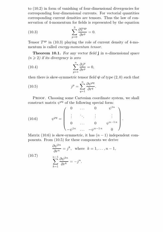
to (10.2) in form of vanishing of four-dimensional divergencies forcorresponding four-dimensional currents. For vectorial quantitiescorresponding current densities are tensors. Thus the law of con-servation of 4-momentum for fields is represented by the equation

(10.3)3∑

p=0

∂T qp

∂rp= 0.

Tensor T qp in (10.3) playing the role of current density of 4-mo-mentum is called energy-momentum tensor.

Theorem 10.1. For any vector field j in n-dimensional space(n > 2) if its divergency is zero

(10.4)n∑

p=1

∂jp

∂rp= 0,

then there is skew-symmetric tensor field ψ of type (2, 0) such that

(10.5) jp =n∑

q=1

∂ψpq

∂rq.

Proof. Choosing some Cartesian coordinate system, we shallconstruct matrix ψpq of the following special form:

(10.6) ψpq =

0 . . . 0 ψ1n

.... . .

......

0 . . . 0 ψn−1 n

−ψ1n . . . −ψn−1 n 0

.

Matrix (10.6) is skew-symmetric, it has (n− 1) independent com-ponents. From (10.5) for these components we derive

(10.7)

∂ψkn

∂rn= jk, where k = 1, . . . , n− 1,

n−1∑k=1

∂ψkn

∂rk= −jn.

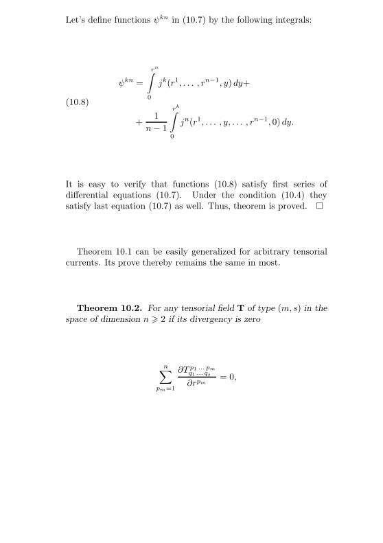
Let’s define functions ψkn in (10.7) by the following integrals:

(10.8)

ψkn =

rn∫0

jk(r1, . . . , rn−1, y) dy+

+1

n− 1

rk∫0

jn(r1, . . . , y, . . . , rn−1, 0) dy.

It is easy to verify that functions (10.8) satisfy first series ofdifferential equations (10.7). Under the condition (10.4) theysatisfy last equation (10.7) as well. Thus, theorem is proved.

Theorem 10.1 can be easily generalized for arbitrary tensorialcurrents. Its prove thereby remains the same in most.

Theorem 10.2. For any tensorial field T of type (m, s) in thespace of dimension n > 2 if its divergency is zero

n∑pm=1

∂T p1 ... pmq1 ... qs

∂rpm= 0,

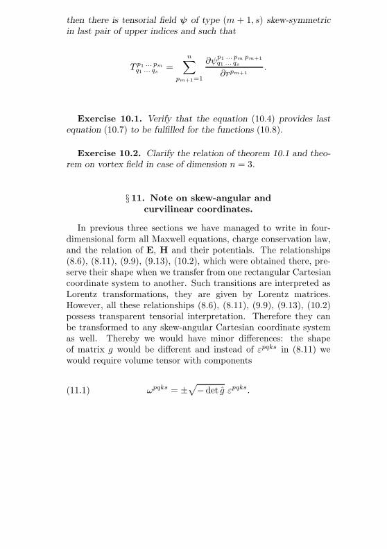
then there is tensorial field ψ of type (m + 1, s) skew-symmetricin last pair of upper indices and such that

T p1 ... pmq1 ... qs

=n∑

pm+1=1

∂ψp1 ... pm pm+1q1 ... qs

∂rpm+1.

Exercise 10.1. Verify that the equation (10.4) provides lastequation (10.7) to be fulfilled for the functions (10.8).

Exercise 10.2. Clarify the relation of theorem 10.1 and theo-rem on vortex field in case of dimension n = 3.

§ 11. Note on skew-angular andcurvilinear coordinates.

In previous three sections we have managed to write in four-dimensional form all Maxwell equations, charge conservation law,and the relation of E, H and their potentials. The relationships(8.6), (8.11), (9.9), (9.13), (10.2), which were obtained there, pre-serve their shape when we transfer from one rectangular Cartesiancoordinate system to another. Such transitions are interpreted asLorentz transformations, they are given by Lorentz matrices.However, all these relationships (8.6), (8.11), (9.9), (9.13), (10.2)possess transparent tensorial interpretation. Therefore they canbe transformed to any skew-angular Cartesian coordinate systemas well. Thereby we would have minor differences: the shapeof matrix g would be different and instead of εpqks in (8.11) wewould require volume tensor with components

(11.1) ωpqks = ±√− det g εpqks.

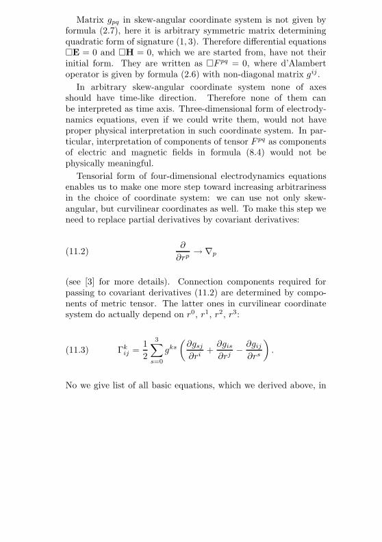
Matrix gpq in skew-angular coordinate system is not given byformula (2.7), here it is arbitrary symmetric matrix determiningquadratic form of signature (1, 3). Therefore differential equationsE = 0 and H = 0, which we are started from, have not theirinitial form. They are written as F pq = 0, where d’Alambertoperator is given by formula (2.6) with non-diagonal matrix gij .

In arbitrary skew-angular coordinate system none of axesshould have time-like direction. Therefore none of them canbe interpreted as time axis. Three-dimensional form of electrody-namics equations, even if we could write them, would not haveproper physical interpretation in such coordinate system. In par-ticular, interpretation of components of tensor F pq as componentsof electric and magnetic fields in formula (8.4) would not bephysically meaningful.

Tensorial form of four-dimensional electrodynamics equationsenables us to make one more step toward increasing arbitrarinessin the choice of coordinate system: we can use not only skew-angular, but curvilinear coordinates as well. To make this step weneed to replace partial derivatives by covariant derivatives:

(11.2)∂

∂rp→ ∇p

(see [3] for more details). Connection components required forpassing to covariant derivatives (11.2) are determined by compo-nents of metric tensor. The latter ones in curvilinear coordinatesystem do actually depend on r0, r1, r2, r3:

(11.3) Γkij =

12

3∑s=0

gks

(∂gsj

∂ri+∂gis

∂rj− ∂gij

∂rs

).

No we give list of all basic equations, which we derived above, in

covariant form. Maxwell equations are written as follows:

(11.4)

3∑q=0

∇qFpq = −4π

cjp,

3∑q=0

3∑k=0

3∑s=0

ωpqks∇qFks = 0.

Here components of volume tensor ωpqks are given by formula(11.1). Tensor of electromagnetic field is expressed through four-dimensional vector-potential by formula

(11.5) Fpq = ∇pAq −∇qAp,

while gauge uncertainty in the choice of vector-potential itself isdescribed by the relationship

(11.6) Ak → Ak +∇kψ,

where ψ is arbitrary scalar field. Charge conservation law incurvilinear coordinates is written as

(11.7)3∑

p=0

∇pjp = 0.

Instead of formula (2.6) for D’Alambert operator here we have

(11.8) =3∑

i=0

3∑j=0

gij ∇i∇j .

Dynamics of material point of nonzero mass m 6= 0 is described

by ordinary differential equations of Newtonian type:

r = u, ∇su =Fmc

.(11.9)

Here dot means standard differentiation with respect to naturalparameter s on world line, while ∇s is covariant derivative withrespect to the same parameter.

Exercise 11.1. Using symmetry of Christoffel symbols (11.3)with respect to lower pair of indices i and j, show that the re-lationship (11.5) can be brought to the form (9.9) in curvilinearcoordinate system as well.

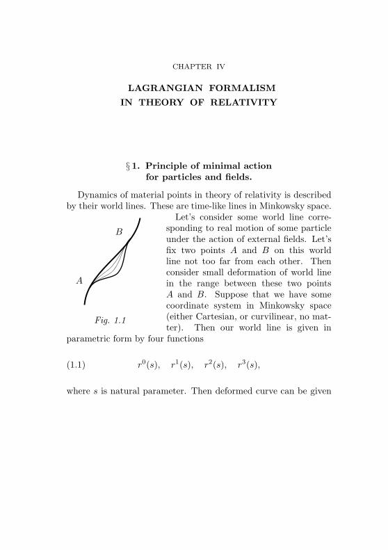
CHAPTER IV

LAGRANGIAN FORMALISM

IN THEORY OF RELATIVITY

§ 1. Principle of minimal actionfor particles and fields.

Dynamics of material points in theory of relativity is describedby their world lines. These are time-like lines in Minkowsky space.

Let’s consider some world line corre-

Fig. 1.1

A

B sponding to real motion of some particleunder the action of external fields. Let’sfix two points A and B on this worldline not too far from each other. Thenconsider small deformation of world linein the range between these two pointsA and B. Suppose that we have somecoordinate system in Minkowsky space(either Cartesian, or curvilinear, no mat-ter). Then our world line is given in

parametric form by four functions

(1.1) r0(s), r1(s), r2(s), r3(s),

where s is natural parameter. Then deformed curve can be given

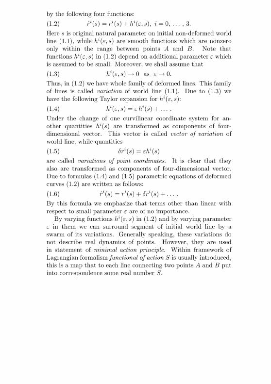
by the following four functions:(1.2) ri(s) = ri(s) + hi(ε, s), i = 0, . . . , 3.Here s is original natural parameter on initial non-deformed worldline (1.1), while hi(ε, s) are smooth functions which are nonzeroonly within the range between points A and B. Note thatfunctions hi(ε, s) in (1.2) depend on additional parameter ε whichis assumed to be small. Moreover, we shall assume that(1.3) hi(ε, s) → 0 as ε→ 0.Thus, in (1.2) we have whole family of deformed lines. This familyof lines is called variation of world line (1.1). Due to (1.3) wehave the following Taylor expansion for hi(ε, s):(1.4) hi(ε, s) = ε hi(s) + . . . .

Under the change of one curvilinear coordinate system for an-other quantities hi(s) are transformed as components of four-dimensional vector. This vector is called vector of variation ofworld line, while quantities(1.5) δri(s) = εhi(s)are called variations of point coordinates. It is clear that theyalso are transformed as components of four-dimensional vector.Due to formulas (1.4) and (1.5) parametric equations of deformedcurves (1.2) are written as follows:

(1.6) ri(s) = ri(s) + δri(s) + . . . .

By this formula we emphasize that terms other than linear withrespect to small parameter ε are of no importance.

By varying functions hi(ε, s) in (1.2) and by varying parameterε in them we can surround segment of initial world line by aswarm of its variations. Generally speaking, these variations donot describe real dynamics of points. However, they are usedin statement of minimal action principle. Within framework ofLagrangian formalism functional of action S is usually introduced,this is a map that to each line connecting two points A and B putinto correspondence some real number S.

Principle of minimal action for particles. World line con-necting two points A and B describes real dynamics of materialpoint if and only if action functional S reaches local minimum onit among other lines being its small variations.

Action functional S producing number by each line should de-pend only on that line (as geometric set of points in M), butit should not depend on coordinate system (r0, r1, r2, r3) in M .By tradition this condition is called Lorentz invariance, thoughchanges of one curvilinear coordinate system by another formmuch broader class of transformations than Lorentz transforma-tions relating two rectangular Cartesian coordinate systems inMinkowsky space.

Action functional in most cases is integral. For single point ofmass m in electromagnetic field with potential A it is written as

(1.7) S = −mcs2∫

s1

ds− q

c

s2∫s1

g(A,u) ds.

Here q is electric charge of particle, while u = u(s) is vector ofits 4-velocity (unit tangent vector of world line). First integralin (1.7) yields action for free particle (in the absence of exter-nal fields), second integral describes interaction of particle withelectromagnetic field.

If we consider system of N particles, then we should writeintegral (1.7) for each of them and we should add all theseintegrals. And finally, in order to get the action functional fortotal system of field and particles we should add integral of action

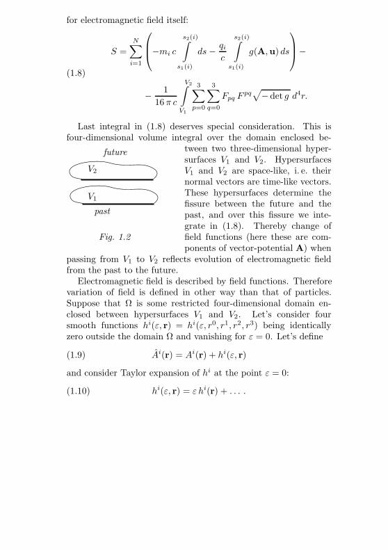
for electromagnetic field itself:

(1.8)

S =N∑

i=1

−mi c

s2(i)∫s1(i)

ds− qic

s2(i)∫s1(i)

g(A,u) ds

−

− 116 π c

V2∫V1

3∑p=0

3∑q=0

Fpq Fpq√− det g d4r.

Last integral in (1.8) deserves special consideration. This isfour-dimensional volume integral over the domain enclosed be-

tween two three-dimensional hyper-surfaces V1 and V2. Hypersurfaces

Fig. 1.2

past

V1

V2

future

V1 and V2 are space-like, i. e. theirnormal vectors are time-like vectors.These hypersurfaces determine thefissure between the future and thepast, and over this fissure we inte-grate in (1.8). Thereby change offield functions (here these are com-ponents of vector-potential A) when

passing from V1 to V2 reflects evolution of electromagnetic fieldfrom the past to the future.

Electromagnetic field is described by field functions. Thereforevariation of field is defined in other way than that of particles.Suppose that Ω is some restricted four-dimensional domain en-closed between hypersurfaces V1 and V2. Let’s consider foursmooth functions hi(ε, r) = hi(ε, r0, r1, r2, r3) being identicallyzero outside the domain Ω and vanishing for ε = 0. Let’s define

(1.9) Ai(r) = Ai(r) + hi(ε, r)

and consider Taylor expansion of hi at the point ε = 0:

(1.10) hi(ε, r) = ε hi(r) + . . . .

The following functions determined by linear terms in the aboveTaylor expansions (1.10)

(1.11) δAi(r) = ε hi(r)

are called variations of field functions for electromagnetic field.Deformation of vector-potential (1.9) now can be written as

(1.12) Ai(r) = Ai(r) + δAi(r) + . . . .

Principle of minimal action for fields. Field functions de-termine actual configuration of physical fields if and only if theyrealize local minimum of action functional S in class of all varia-tions with restricted support*.

The condition of minimum of action for actual field configura-tion and for actual world lines of particles, as a rule, is not used.In order to derive dynamical equations for fields and particles it issufficient to have extremum condition (no matter minimum, max-imum, or saddle point). For this reason minimal action principleoften is stated as principle of extremal action.

Exercise 1.1. Verify that hi(s) in (1.4) are transformed ascomponents of vector under the change of coordinates.

Exercise 1.2. Prove that under gauge transformations (11.6)from Chapter III action functional (1.8) is transformed as follows:

(1.13) S → S −N∑

i=1

(qicψ(r(s2(i)))− qi

cψ(r(s1(i)))

).

Explain why terms added to action functional in (1.13) are notsensitive to variation of word lines (1.2).

* Variations with restricted support are those which are identically zerooutside some restricted domain Ω.

§ 2. Motion of particle in electromagnetic field.

In order to find world line of relativistic particle in externalelectromagnetic field we shall apply particle version of extremalaction principle to functional (1.8). Let’s choose one of N par-ticles in (1.8) and consider deformation (1.6) of its world line.When we substitute deformed world line into (1.8) in place ofinitial non-deformed one the value of last integral remains un-changed. Thereby in first term containing sum of integrals onlyone summand changes its value, that one which represent the par-ticle we have chosen among others. Therefore writing extremitycondition for (1.8) we can use action functional in form of (1.7).The value of (1.7) for deformed world line is calculated as follows:

(2.1) Sdef = −mcs2∫

s1

√g(K,K) ds− q

c

s2∫s1

g(A,K) ds.

Formula (2.1) visually differs from formula (1.7) because s isnatural parameter on initial world line, but it is not naturalparameter on deformed line. Here tangent vector

(2.2) K(s) =dr(s)ds

= u(s) + εdh(s)ds

+ . . .

is not unit vector. Therefore first integral (1.7) is rewritten aslength integral (see (6.4) in Chapter III). In second integral (1.7)unit tangent vector is replaced by vector K.

Let’s write in coordinate form both expressions which are underintegration in (2.1) taking into account that we deal with generalcurvilinear coordinate system in Minkowsky space:

(2.3)

√g(K,K) =

√√√√ 3∑i=0

3∑j=0

gij(r(s))Ki(s)Kj(s),

g(A,K) =3∑

i=0

Ai(r(s))Ki(s).

Let’s substitute (2.2) into (2.3) and take into account (1.2) andthe expansion (1.4). As a result for the expressions (2.3) we getthe following power expansions with respect to small parameter ε:

√g(K,K) =

√g(u,u) +

ε√g(u,u)

(3∑

i=0

ui(s)dhi(s)ds

+

+12

3∑i=0

3∑j=0

3∑k=0

∂gij

∂rkui(s)uj(s)hk(s)

)+ . . . ,

g(A,K) = g(A,u) + ε

3∑i=0

Ai(r(s))dhi(s)ds

+

+ ε

3∑i=0

3∑k=0

∂Ai

∂rkui(s)hk(s) + . . . .

When substituting these expansions into (2.1) we should remem-ber that u is unit vector. Then for Sdef we get

Sdef = S − ε

s2∫s1

3∑k=0

(mcuk(s) +

q

cAk(r(s))

) dhk(s)ds

ds−

− ε

s2∫s1

3∑k=0

(q

c

3∑i=0

∂Ai

∂rkui +

mc

2

3∑i=0

3∑j=0

∂gij

∂rkuiuj

)hk(s) ds+ . . . .

Let’s apply integration by parts to first integral above. As a result

we get the expression without derivatives of functions hk(s):

Sdef = S − ε

3∑k=0

(mcuk(s) +

q

cAk(r(s))

)hk(s)

s2

s1

+

+ ε

s2∫s1

3∑k=0

d

ds

(mcuk(s) +

q

cAk(r(s))

)hk(s) ds−

− ε

s2∫s1

3∑k=0

(q

c

3∑i=0

∂Ai

∂rkui +

mc

2

3∑i=0

3∑j=0

∂gij

∂rkuiuj

)hk(s) ds+ . . . .

Remember that function hk(s) vanish at the ends of integrationpath hk(s1) = hk(s2) = 0 (see § 1). This provides vanishing ofnon-integral terms in the above formula for Sdef.

Now in order to derive differential equations for world line ofparticle we apply extremity condition for S. It means that termlinear with respect to ε in power expansion for Sdef should beidentically zero irrespective to the choice of functions hk(s):

(2.4)

d

ds

(mcuk(s) +

q

cAk(r(s))

)=

=q

c

3∑i=0

∂Ai

∂rkui +

mc

2

3∑i=0

3∑j=0

∂gij

∂rkui uj.

Let’s calculate derivative in left hand side of (2.4). Then let’srearrange terms so that those with mc factor are in left handside, while others with q/c factor are in right hand side:

mc

(duk

ds− 1

2

3∑i=0

3∑j=0

∂gij

∂rkui uj

)=q

c

3∑i=0

(∂Ai

∂rk− ∂Ak

∂ri

)ui.

Now in right hand side of this equation we find tensor of electro-magnetic field (see formula (9.9) in Chapter III). For transformingleft hand side of this equation we use formula (11.3) from Chap-ter III. As a result we get the following equation for world line:

(2.5) mc

(duk

ds−

3∑i=0

3∑j=0

Γikj ui u

j

)=q

c

3∑i=0

Fki ui.

In left hand side of the equation (2.5) we find covariant derivativewith respect to parameter s along world line:

(2.6) mc∇suk =q

c

3∑i=0

Fki ui.

Comparing (2.6) with the equations (11.9) from Chapter III, we

get formula for the vector of four-dimensional force acting on aparticle with charge q in electromagnetic field:

(2.7) Fk =q

c

3∑i=0

Fki ui.

Suppose that we have rectangular Cartesian coordinate systemin Minkowsky space. Then we can subdivide F into spatial andtemporal parts and can calculate components of three-dimensionalforce vector: f i =

√c2 − |v|2 F i (see formula (7.6) in Chap-

ter III). Upon easy calculations with the use of formulas (7.2) and(9.4) from Chapter III for force vector f we get

(2.8) f = qE +q

c[v, H].

This formula (2.8) is exactly the same as formula for Lorentz force(see (4.4) in Chapter I). Thus formula (2.7) is four-dimensionalgeneralization of formula for Lorentz force. Orthogonality condi-tion for 4-force and 4-velocity (see (7.5) in Chapter III) for (2.7) isfulfilled due to skew symmetry of tensor of electromagnetic field.

Exercise 2.1. Prove that gauge transformation of action func-tional (1.13) does not change dynamic equations of material pointin electromagnetic field (2.6).

Exercise 2.2. Verify that the relationship (7.5) from Chap-ter III holds for Lorentz force.

§ 3. Dynamics of dust matter.

Differential equation (2.6) describes motion of charged particlesin electromagnetic field. If the number of particles is not large,then we can follow after the motion of each of them. Whendescribing extremely large number of particles continual limit isused, particles are replaced by continuous medium modeling their

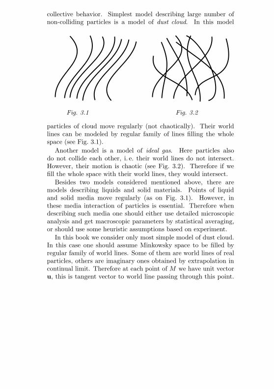
collective behavior. Simplest model describing large number ofnon-colliding particles is a model of dust cloud. In this model

Fig. 3.1 Fig. 3.2

particles of cloud move regularly (not chaotically). Their worldlines can be modeled by regular family of lines filling the wholespace (see Fig. 3.1).

Another model is a model of ideal gas. Here particles alsodo not collide each other, i. e. their world lines do not intersect.However, their motion is chaotic (see Fig. 3.2). Therefore if wefill the whole space with their world lines, they would intersect.

Besides two models considered mentioned above, there aremodels describing liquids and solid materials. Points of liquidand solid media move regularly (as on Fig. 3.1). However, inthese media interaction of particles is essential. Therefore whendescribing such media one should either use detailed microscopicanalysis and get macroscopic parameters by statistical averaging,or should use some heuristic assumptions based on experiment.

In this book we consider only most simple model of dust cloud.In this case one should assume Minkowsky space to be filled byregular family of world lines. Some of them are world lines of realparticles, others are imaginary ones obtained by extrapolation incontinual limit. Therefore at each point of M we have unit vectoru, this is tangent vector to world line passing through this point.

This means that dynamics of dust cloud can be described byvector field u(r).

Apart from vector field u, below we need scalar parameter ν(r)which means the density of dust cloud. We define it as follows.Let’s choose some small fragment of three-dimensional hypersur-face in M orthogonal to vector u(r) at the point r. The numberof dust particles whose world lines cross this fragment is propor-tional to its three-dimensional volume: N = ν(r)V , parameterν(r) is coefficient of proportionality. Parameter ν(r) has measureunit of concentration, it can be treated as concentration of par-ticles in small fragment of dust cloud near the point r measuredin that inertial coordinate system for which particles of this smallfragment are at rest. By means of ν(r) and u(r) we compose newfour-dimensional vector

(3.1) η(r) = c ν(r)u(r).

Vector (3.1) is called four-dimensional flow density for particlesin cloud. If we choose some inertial coordinate system, thenη0/c is interpreted as concentration of particles in dust cloud,while other three components of four-dimensional vector η formthree-dimensional vector of flow density.

Suppose that dust cloud is formed by identical particles withmass m and charge q. Then four-dimensional current densityvector can be represented as follows:

(3.2) j(r) = q η(r).

By analogy with (3.2) one can define mass flow density vector:

(3.3) µ(r) = mη(r).

Total number of particles in cloud is fixed. This conservation lawis written as the following equality for η:

(3.4)3∑

p=0

∇pηp = 0.

From (3.4) and (3.2) one can derive charge conservation law inform of the relationship (11.7) from Chapter III. Taking intoaccount (3.3), we get rest mass conservation law:

(3.5)3∑

p=0

∇pµp = 0.

Rest mass conservation law here is fulfilled due to the absence ofcollisions when heavy particles can be produced from light ones(see § 7 in Chapter III).

Let’s consider dynamics of particles composing dust cloud.Vector field u is constituted by tangent vectors to world linesof dust particles. Therefore these world lines can be determinedas integral curves of vector field u, i. e. by solving the followingsystem of ordinary differential equations:

(3.6)dri

ds= ui(r(s)), i = 0, . . . , 3.

Having determined world line of particle from differential equa-tions, we know vector of its 4-velocity u(s). Now let’s calculatecovariant derivative of vector u(s) with respect to parameter s:

(3.7) ∇sup =

dup(s)ds

+3∑

k=0

3∑n=0

Γpnk u

k(s)un(s).

Calculating derivative dup/ds in (3.7) we take into account (3.6)and the equality u(s) = u(r(s)). As a result we get

(3.8)dup(s)ds

=3∑

k=0

uk ∂up

∂rk.

Substituting (3.8) into (3.7), we derive the following formula:

(3.9) ∇sup =

3∑k=0

uk∇kup.

Right hand side of (3.9) is covariant derivative of vector field u(r)along itself (see more details in [3]). Substituting (3.9) into theequations of the dynamics of material point, we get:

(3.10) ∇uu =Fmc

.

Here F = F(r,u) is some external force field acting on particlesof dust matter. For example in the case of charged dust inelectromagnetic field the equation (3.10) looks like

(3.11)3∑

k=0

uk∇kup =q

mc2

3∑k=0

Fpk uk.

In contrast to the equations (11.9) from Chapter III, whichdescribe dynamics of separate particle, here (3.10) are partialdifferential equations with respect to components of vector fieldu(r). They describe dynamics of dust cloud in continual limit.The equation for scalar field ν(r) is derived from conservation law(3.4) for the number of particles. Combining these two equations,we obtain a system of differential equations:

(3.12)

3∑k=0

uk∇kup =Fp

mc,

3∑k=0

uk∇kν = −ν3∑

k=0

∇kuk.

System of partial differential equations (3.12) yields completedescription for the dynamics of dust cloud.

Model of dust matter cam be generalized a little bit. We canconsider mixture of particles of different sorts. For each sort ofparticles we define its own vector field u(i, r) and its own scalar

field of concentration ν(i, r). Then formulas (3.2) and (3.3) for jand µ are generalized as follows:

j(r) =n∑

i=1

q(i)η(i, r), µ(r) =n∑

i=1

m(i)η(i, r).

Here η(i, r) = c ν(i, r)u(i, r). Each pair of fields u(i, r) and ν(i, r)satisfies differential equations (3.12). We can derive mass andcharge conservation laws from these equations.

§ 4. Action functional for dust matter.

Let’s study the dynamics of dust matter in electromagneticfield within framework of Lagrangian formalism. Fort this purposewe need to pass to continual limit in action functional (1.8).For the sake of simplicity we consider dust cloud with identicalparticles. Omitting details of how it was derived, now we writeultimate formula for action functional (1.8) in continual limit:

(4.1)

S = −mV2∫

V1

√g(η,η)

√− det g d4r−

− q

c2

V2∫V1

g(η,A)√− det g d4r−

− 116π c

V2∫V1

3∑p=0

3∑k=0

Fpk Fpk√− det g d4r.

Instead of deriving formula (4.1) from (1.8) we shall verify thisformula indirectly. For this purpose we shall derive dynamicalequation (3.11) from principle of extremal action applied to actionfunctional (4.1).

For describing dust matter in (4.1) we have chosen vector fieldη(r) defined in (3.1). Other two fields u(r) and ν(r) can beexpressed though vector field η(r):

c ν = |η| =√g(η,η) , u =

η

c ν.(4.2)

Dealing with variation of vector field η(r) we should alwaysremember that components of this field are not independentfunctions. They satisfy differential equation (3.4). In orderto resolve tis equation (3.4) we use slightly modified version oftheorem 10.1 from Chapter III.

Theorem 4.1. Let M be some n-dimensional manifold, wheren ≥ 2, equipped with metric gij . For each vector field η with zero

divergency with respect to metric connection

(4.3)n∑

p=1

∇pηp = 0

there is skew-symmetric tensor field ϕ of type (2, 0) such that thefollowing relationships are fulfilled

(4.4) ηp =n∑

q=1

∇qϕpq.

Proof. Writing relationships (4.3), we use well-known for-mula for components of metric connection, see formula (11.3) inChapter III. As a result we get

n∑p=1

∇pηp =

n∑p=1

∂ηp

∂rp+

n∑p=1

n∑s=1

Γpps η

s =n∑

p=1

∂ηp

∂rp+

+12

n∑p=1

n∑s=1

n∑k=1

gpk

(∂gpk

∂rs+∂gks

∂rp− ∂gps

∂rk

)ηs.

Note that last two derivatives of metric tensor in round bracketsare canceled when we sum over indices p and k. This is becausegpk is symmetric. Hence

(4.5)

n∑p=1

∇pηp =

n∑p=1

∂ηp

∂rp+

12

n∑p=1

n∑s=1

n∑k=1

gsk ∂gks

∂rpηp =

=n∑

p=1

∂ηp

∂rp+

12

n∑p=1

tr(g−1 ∂g

∂rp

)ηp.

For further transforming of this expression (4.5) we use wellknown formula for logarithmic derivative of determinant:

(4.6)∂ ln | det g|

∂rp= tr

(g−1 ∂g

∂rp

).

Substituting (4.6) into (4.5), we transform (4.5) so that

(4.7)n∑

p=1

∇pηp =

1√| det g|n∑

p=1

∂(ηp√| det g|)∂rp

.

Let’s carry out analogous calculations for right hand side of (4.4)taking into account skew symmetry of the field ϕpq and symmetryof connection components Γk

pq. These calculations yield

(4.8)n∑

q=1

∇qϕpq =

1√| det g|n∑

q=1

∂(ϕpq√| det g|)∂rq

.

Denote jp =√| det g| ηp and ψpq =

√| det g|ϕpq. Now on thebase of (4.7) and (4.8) it is easy to understand that proof oftheorem 4.1 is reduced to theorem 10.1 from Chapter III.

Remark. Generally speaking, theorem 10.2 has no directgeneralization for the case of spaces with metric. It is generalizedonly for metric spaces with zero curvature tensor Rs

kpq = 0.

Let’s define deformation of the field η in a way similar to thatwe used for vector-potential A in § 1:

(4.9) ηp(r) = ηp(r) + ε ζp(r) + . . . .

Both fields η and η satisfy differential equation (3.4). Hencevector field ζ defined in (4.9) also satisfy this equation. Let’s

apply theorem 4.1 to vector field ζ:

(4.10) ζp =3∑

k=0

∇kϕpk.

Theorem 4.1 does not specify tensor field ϕpk in (4.10), this canbe any skew-symmetric tensor field. However, we choose it in veryspecial form as follows:

(4.11) ϕpk = ηp hk − hp ηk.

This choice can be motivated by the following theorem.

Theorem 4.2. For any two vector fields ζ and η, where η 6= 0,both satisfying differential equation (3.4) there is vector field hsuch that vector field ζ is given by formula

ζp =3∑

k=0

∇k(ηp hk − hp ηk).

Our choice (4.11) leads to the following expression for the field η:

(4.12) ηp(r) = ηp(r) + ε3∑

k=0

∇k(ηp hk − hp ηk) + . . . .

Quantities hi(r) in (4.12) are chosen to be smooth functions beingnonzero only within some restricted domain Ω in Minkowskyspace.

When substituting (4.12) into action functional (4.1) we usethe following expansion for

√g(η, η) :

√g(η, η) =

√g(η,η) +

ε√g(η,η)

3∑p=0

3∑q=0

ηp∇kϕpk + . . . .

We have analogous power expansion for the expression undersecond integral in formula (4.1):

g(η,A) = g(η,A) + ε

3∑p=0

3∑k=0

Ap∇kϕpk + . . . .

Substituting these two expansions into (4.1), we take into account(4.2). For the action Sdef this yields

(4.13)

Sdef = S − εm

∫Ω

3∑p=0

3∑k=0

up∇kϕpk√− det g d4r−

− ε q

c2

∫Ω

3∑p=0

3∑k=0

Ap∇kϕpk√− det g d4r + . . . .

Further in order to transform the above expression (4.13) weuse Ostrogradsky-Gauss formula. In the space equipped withmetric this formula is written as follows:

(4.14)∫Ω

3∑k=0

∇kzk√− det g d4r =

∫∂Ω

g(z,n) dV.

Here z0, z1, z2, z3 are components of smooth vector field z,while n is unit normal vector for the boundary of the domainΩ. In order to transform first integral in formula (4.13) we takezk =

∑3p=0 up ϕ

pk. Then in right hand side of (4.14) we obtain

3∑k=0

∇kzk =

3∑p=0

3∑k=0

up∇kϕpk +

3∑p=0

3∑k=0

∇kup ϕpk.

Right hand side of (4.14) vanishes since ϕpk do vanish on theboundary of Ω. Hence we have the equality∫

Ω

3∑p=0

3∑k=0

up∇kϕpk√− det g d4r =

−∫Ω

3∑p=0

3∑k=0

∇kup ϕpk√− det g d4r.

In a similar way we transform second integral in (4.13). In wholefor the action Sdef we get the following expression

(4.15)

Sdef = S + εm

∫Ω

3∑p=0

3∑k=0

∇kup ϕpk√− det g d4r+

+ε q

c2

∫Ω

3∑p=0

3∑k=0

∇kAp ϕpk√− det g d4r + . . . .

Extremity of action S means that linear part with respect to εin formula (4.15) should vanish:∫

Ω

3∑p=0

3∑k=0

(m∇kup +

q

c2∇kAp

)ϕpk√− det g d4r = 0.

Let’s substitute formula (4.11) for ϕpk into the above equality.Then it is transformed to the following one∫

Ω

3∑p=0

3∑k=0

(m∇kup +

q

c2∇kAp

)ηphk

√− det g d4r =

=∫Ω

3∑p=0

3∑k=0

(m∇kup +

q

c2∇kAp

)ηkhp

√− det g d4r.

Let’s exchange indices k and p in second integral. Thereafterintegrals can be united into one integral:

(4.16)

∫Ω

3∑k=0

3∑p=0

(m∇kup −m∇puk +

q

c2∇kAp−

− q

c2∇pAk

)ηphk

√− det g d4r = 0.

Now let’s take into account that in resulting equality hk = hk(r)are arbitrary smooth functions vanishing outside the domain Ω.Therefore vanishing of integral (4.16) means vanishing of eachsummand in sum over index k in the expression under integration:

(4.17)3∑

p=0

(m∇kup −m∇puk +

q

c2Fkp

)ηp = 0.

Here we used the relationship (11.5) from Chapter III. It re-lates tensor of electromagnetic field and four-dimensional vector-potential.

In order to bring the equation (4.17) just derived to its ultimateform we use the relationships (4.2), which relate vector field ηand vector field u: ηp = c ν up. Since u is unit vector, we have

(4.18)3∑

p=0

up∇kup = 0.

Taking into account (4.18), we bring (4.17) to the following form:

(4.19)3∑

p=0

up∇puk =q

mc2

3∑p=0

Fkp up.

Now it is easy to see that (4.19) exactly coincides with the equa-tion (3.11), which we have derived earlier. This result approvesthe use of the action (4.1) for describing charged dust matter inelectromagnetic field.

Exercise 4.1. Prove that for any skew-symmetric tensor fieldϕpq vector field η determined by formula (4.4) has zero divergency,i. e. is satisfies differential equation (3.4).

Exercise 4.2. Prove theorem 4.2. For this purpose use thefollowing fact known as theorem on rectification of vector field.

Theorem 4.3. For any vector field η 6= 0 there exists somecurvilinear coordinate system r0, r1, r2, r3 such that η0 = 1,η1 = 0, η2 = 0, η3 = 0 in this coordinate system.

Exercise 4.3. Prove theorem 4.3 on rectification of vector field.

Exercise 4.4. Derive Ostrogradsky-Gauss formula (4.14) forthe space equipped with metric on the base of the following integralrelationship in standard space Rn:∫

Ω

∂f(r)∂ri

dnr =∫

∂Ω

f(r) dr1 . . . dri−1dri+1 . . . drn.

§ 5. Equations for electromagnetic field.

In this section we continue studying action functional (4.1).This functional describes dust cloud composed of particles withmass m and charge q in electromagnetic field. In previous sectionwe have found that applying extremal action principle to S with

respect to the field η one can derive dynamical equations forvelocity field in dust cloud. Now we shall apply extremal actionprinciple to S with respect to vector-potential A. Deformation ofvector-potential is defined according to (1.9), (1.10), (1.11), (1.12):

(5.1) Ai(r) = Ai(r) + εhi(r) + . . . .

For components of tensor of electromagnetic field we derive

(5.2) Fij = Fij + ε (∇ihj −∇jhi) + . . . .

When substituting (5.2) into action functional (4.1) we carry outthe following calculations:

3∑p=0

3∑k=0

Fpk Fpk =

3∑i=0

3∑j=0

3∑p=0

3∑k=0

Fpk Fij gpi gkj =

=3∑

p=0

3∑k=0

Fpk Fpk + 2 ε

3∑p=0

3∑k=0

F pk(∇phk −∇khp) + . . . .

Taking into account skew symmetry of tensor F pk, this expansioncan be simplified more and can be brought to the form

3∑p=0

3∑k=0

Fpk Fpk =

3∑p=0

3∑k=0

Fpk Fpk + 4 ε

3∑p=0

3∑k=0

F pk∇phk + . . . .

Analogous calculations in substituting (5.1) into (4.1) yield

g(η, A) = g(η,A) + ε

3∑k=0

ηk hk + . . . .

As a result for deformation of action functional (4.1) we get

Sdef = S − εq

c2

∫Ω

3∑k=0

ηk hk

√− det g d4r−

− ε

4π c

∫Ω

3∑p=0

3∑k=0

F pk∇phk

√− det g d4r + . . . .

Let’s transform second integral in the above expansion for Sdef

by means of Ostrogradsky-Gauss formula (4.14). For this purposelet’s choose zp =

∑3k=0 F

pkhk and take into account vanishing ofhk on the boundary of the domain Ω. Then for Sdef we get

Sdef = S + ε

∫Ω

3∑k=0

(−qη

k

c2+

3∑p=0

∇pFpk

4π c

)hk

√− det g d4r + . . . .

Extremal action principle means that linear in ε part of the aboveexpansion for Sdef should vanish. Note also that Ω is an arbitrarydomain and hk(r) are arbitrary functions within Ω. This yieldthe following equations for the tensor of electromagnetic field:

(5.3)3∑

p=0

∇pFpk =

4π qc

ηk.

Remember that η(r) is related to current density by means of(3.2). Then (5.3) can be written as

(5.4)3∑

p=0

∇pFkp = −4π

cjk.

It is easy to see that (5.4) are exactly Maxwell equations writtenin four-dimensional form (see (11.4) in Chapter III). Another pairof Maxwell equations written in four-dimensional form

3∑q=0

3∑k=0

3∑s=0

ωpqks∇qFks = 0

is a consequence of the relationship Fpq = ∇pAq − ∇qAp (seeformula (11.5) in Chapter III).

Exercise 5.1. Which form will have differential equations (5.3)if we consider dust cloud composed by particles of several sortswith masses m(1), . . . , m(N) and charges q(1), . . . , q(N) ? Willthis change differential equations (5.4) ?

CHAPTER V

GENERAL THEORY OF RELATIVITY

§ 1. Transition to non-flat metricsand curved Minkowsky space.

Passing from classical electrodynamics to special theory of re-lativity, in previous two chapters we have successively geometrizedmany basic physical concepts. Having denoted r0 = ct and com-bining r0 with components of three-dimensional radius-vector ininertial coordinate system, we have constructed four-dimensionalspace of events (Minkowsky space). This space appears to beequipped with metric of signature (1, 3), which is called Min-kowsky metric. Thereby inertial coordinate systems are inter-preted as orthonormal bases in Minkowsky metric.

In four-dimensional formalism dynamics of material point isdescribed by vectorial differential equations, while Maxwell equa-tions for electromagnetic field are written in tensorial form. Dueto this circumstance in previous two chapters we managed toinclude into consideration skew-angular and even curvilinear co-ordinate systems in Minkowsky space. Thereby we got explicitentries of metric tensor components gij , metric connection com-ponents Γk

ij , and covariant derivatives ∇i in all our equations.Next step in this direction is quite natural. One should keep

the shape of all equations and pass from flat Minkowsky metric

to metric of signature (1, 3) with nonzero curvature tensor:

(1.1) Rkqij =

∂Γkjq

∂ri− ∂Γk

iq

∂rj+

3∑s=0

Γkis Γs

jq −3∑

s=0

Γkjs Γs

iq.

This crucial step was first made by Einstein. Theory he had dis-covered in this way later was called Einstein’s theory of gravitationor general theory of relativity.

Definition 1.1. Four-dimensional affine space equipped withorientation, polarization, and with metric of signature (1, 3) andnonzero curvature (1.1) is called curved Minkowsky space.

In non-flat Minkowsky space we loose some structures availablein flat case. In such space there are no coordinates for whichMinkowsky metric is given by matrix (2.7) from Chapter III, i. e.here we have no inertial coordinate systems. This is substantialloss, but it is not catastrophic since dynamic equation for materialpoints and Maxwell equations rewritten in vectorial and tensorialform are not bound to inertial coordinate systems.

Geodesic lines in curved Minkowsky space do not coincidewith affine straight lines. Therefore affine structure becomesexcessive restriction in general relativity. As appears, one cangive up topologic structure of flat space R4 as well. Even intwo-dimensional case, as we know, apart from deformed (curved)plain, there are surfaces with more complicated topology: sphere,torus and sphere with several handles glued to it (see [5]). Inmultidimensional case these objects are generalized in concept ofsmooth manifold (see details in [2], [5], and [6]).

Smooth manifold M of dimension n is a topologic space eachpoint of which has a neighborhood (a chart) identical to someneighborhood of a point in Rn. In other words M is covered by afamily of charts Uα, each of which is diffeomorphic to some openset Vα in Rn. Such chart maps (chart diffeomorphisms) definelocal curvilinear coordinate systems within their chart domains

Uα. At those points of manifold M , where two chart domains areoverlapping, transition functions arise. They relate one curvilinearcoordinate system with another:

(1.2)ri = ri(r1, . . . , rn), where i = 1, . . . , n,

ri = ri(r1, . . . , rn), where i = 1, . . . , n.

According to definition of smooth manifold, transition functions(1.2) are smooth functions (of class C∞). Transition functionsdetermine transition matrices S and T :

T ij =

∂ri

∂rj, Si

j =∂ri

∂rj.(1.3)

Presence of transition matrices (1.3) lead to full-scale theory oftensors, which is almost literally the same as theory of tensorsfor curvilinear coordinates in Rn (see [3]). The only differenceis that here we cannot choose Cartesian coordinates at all. Thisis because in general there is no smooth diffeomorphic map frommanifold M to Rn.

Definition 1.1. Four-dimensional smooth manifold equippedwith orientation, polarization, and with metric of signature (1, 3)is called generalized Minkowsky space or Minkowsky manifold.

§ 2. Action for gravitational field.Einstein equation.

Space of events in general relativity is some smooth Minkowskymanifold M . This circumstance provides additional arbitrarinessconsisting in choosing M and in choosing metric on M . Nonzerocurvature described by tensor (1.1) is interpreted as gravitationalfield. Gravitational field acts upon material bodies and uponelectromagnetic field enclosed within M . This action is due tothe presence of covariant derivatives in dynamic equations. Themagnitude of gravitational field itself should be determined by

presence of matter in M in form of massive particles or in form ofelectromagnetic radiation, i. e. we should have backward relationbetween geometry of the space and its content.

In order to describe backward relation between gravitationalfield and other physical fields we use Lagrangian formalism andextremal action principle. Let’s start from action functional (4.1)in Chapter IV. It is sum of three integrals:

(2.1) S = Smat + Sint + Sel.

First integral Smat is responsible for material particles in form ofdust cloud, second integral describes interaction of dust cloud andelectromagnetic field, third term in (2.1) describes electromagneticfield itself. In order to describe gravitational field one moresummand in (2.1) is added:

(2.2) S = Sgr + Smat + Sint + Sel.

This additional term is chosen in the following form:

(2.3) Sgr = − c3

16πγ

V2∫V1

R√− det g d4r.

Here γ gravitational constant same as in Newton’s universal lawof gravitation (see formula (1.11) in Chapter I). Scalar quantity Rin (2.3) is scalar curvature determined by curvature tensor (1.1)according to the following formula:

(2.4) R =3∑

q=0

3∑k=0

3∑j=0

gqjRkqkj .

Ricci tensor is an intermediate object relating curvature tensor(1.1) and scalar quantity (2.4). Here are its components:

(2.5) Rqj =3∑

k=0

Rkqkj .

Ricci tensor is symmetric (see [3]). Scalar curvature R is obtainedby contracting Ricci tensor and metric tensor gqj with respect toboth indices q and j. This fact is obvious due to (2.5) and (2.4).

Note that sometimes in the action for gravitational field (2.3)one more constant parameter Λ is added:

Sgr = − c3

16πγ

V2∫V1

(R+ 2 Λ)√− det g d4r.

This parameter is called cosmological constant. However, accord-ing to contemporary experimental data the value of this constantis undetectably small or maybe is exactly equal to zero. Thereforefurther we shall use action Sgr in form of (2.3).

Note also that metric tensor describing gravitational field entersin implicit form into all summand in (2.2). Therefore we neednot add special terms describing interaction of gravitational fieldwith material particles and electromagnetic field. Moreover, suchadditional terms could change the form of dynamical equations formatter and form of Maxwell equations for electromagnetic fieldthus contradicting our claim that these equations are the same ingeneral and in special relativity.

Now let’s begin with deriving dynamical equations for grav-itational field. For this purpose we consider deformation ofcomponents of metric tensor given by the following relationship:

(2.6) gij(r) = gij(r) + ε hij(r) + . . . .

Functions hij(r) in (2.6) are assumed to be smooth functionsvanishing outside some restricted domain Ω ⊂M . Deformation ofmatrix gij lead to deformation of inverse matrix gij :

(2.7)

gij = gij − ε hij + . . . =

= gij − ε3∑

p=0

3∑q=0

gip hpq gqj + . . . .

Let’s differentiate the relationship (2.7) and let’s express partialderivatives through covariant derivatives in resulting formula:

(2.8)

∂gij

∂rk=∂gij

∂rk−ε ∂hij

∂rk+ . . . =

∂gij

∂rk− ε∇khij+

+ ε

3∑p=0

Γpki hpj + ε

3∑p=0

Γpkj hip + . . . .

In (2.8) we used covariant derivatives corresponding to non-deformed metric gij . Now on the base of (2.8) we calculatethe following combination of derivatives:

(2.9)

∂gkj

∂ri+∂gik

∂rj− ∂gij

∂rk=∂gkj

∂ri+∂gik

∂rj− ∂gij

∂rk−

− ε

(∇ihkj +∇jhik −∇khij − 2

3∑p=0

Γpij hpk

)+ . . . .

Let’s use the relationships (2.6) and (2.8) in calculating defor-mation of connection components. For this purpose let’s applywell-known formula to Γp

ij (see formula (11.3) in Chapter III):

Γpij = Γp

ij +ε

2

3∑k=0

gpk (∇ihkj +∇jhik −∇khij) + . . . .

This expansion for Γpij can be written in symbolic concise form

(2.10) Γpij = Γp

ij + ε Y pij + . . .

by introducing the following quite natural notation:

(2.11) Y pij =

12

3∑k=0

gpk (∇ihkj +∇jhik −∇khij) .

Now let’s substitute the expansion (2.10) into the formula (1.1)for curvature tensor. This yields

(2.12) Rkqij = Rk

qij + ε(∇iY

kjq −∇jY

kiq

)+ . . . .

Upon contracting (2.12) with respect to one pair of indices we getsimilar expansion for deformation of Ricci tensor:

(2.13) Rqj = Rqj + ε3∑

k=0

(∇kYkjq −∇jY

kkq

)+ . . . .

We multiply (2.13) by gqj using formula (2.6). Then we carry outcomplete contraction with respect to both indices q and j. Thisyields deformation of scalar curvature:

R = R+ ε

3∑j=0

3∑q=0

(Rqj h

qj +3∑

k=0

gqj(∇kYkjq −∇jY

kkq)

)+ . . . .

Let’s introduce vector field with the following components:

Zk =3∑

j=0

3∑q=0

(Y k

jqgqj − Y j

jqgqk).

Then we can rewrite deformation of scalar curvature R as

(2.14) R = R+ ε3∑

j=0

3∑q=0

Rqj hqj + ε

3∑k=0

∇kZk + . . . .

When substituting (2.14) into action integral (2.3) we should notethat second sum in (2.14) is exactly covariant divergency of vectorfield Z. Components of Z are smooth functions vanishing outsidethe domain Ω. Therefore integral of such sum is equal to zero:∫

Ω

3∑k=0

∇kZk√− det g d4r =

∫∂Ω

g(Z,n) dV = 0.

This follows from Ostrogradsky-Gauss formula (see (4.14) inChapter IV). Hence for deformation of Sgr we get

Sdef = Sgr− ε c3

16πγ

∫Ω

3∑j=0

3∑q=0

(Rqj − R

2gqj

)hqj√− det g d4r+ . . . .

In deriving this formula we also used the following expansion:

(2.15)√− det g =

√− det g

(1− ε

3∑j=0

3∑q=0

gqj hqj

2

)+ . . . .

It follows from (2.6). Now we shall not calculate deformations ofother three terms in (2.2) in explicit form. This will be done in§ 4 and § 5 below. However, we introduce notation

(2.16) Sm.f. = Smat + Sint + Sel.

Here Sm.f. denotes overall action for all material fields other thangravitation. The number of terms in the sum (2.16) could be muchmore than three, if one consider more complicated models fordescribing matter. But in any case action of gravitational field isexcluded from this sum since gravitational field plays exceptionalrole in general relativity. Now we shall write deformation of theaction (2.16) in the following conditional form:

(2.17) Sdef = Sm.f. +ε

2c

∫Ω

3∑q=0

3∑j=0

Tqj hqj√− det g d4r + . . . .

Then extremity condition for total action (2.2) is written as

(2.18) Rqj − R

2gqj =

8πγc4

Tqj .

This equation (2.18) is known as Einstein equation. It is ba-sic equation describing dynamics of metric tensor gij in generaltheory of relativity.

Exercise 2.1. Derive the relationships (2.7) and (2.15) fromthe expansion (2.6) for deformation of tensor gij .

§ 3. Four-dimensional momentumconservation law for fields.

Tensor T in right hand side of Einstein equation (2.18) is calledenergy-momentum tensor for material fields. It is determinedby the relationship (2.17) and comprises contributions from allmaterial fields and their interactions. In the model of dust matterin electromagnetic field tensor T is composed of three parts (seeformula (2.16)).

Energy-momentum tensor is related with 4-momentum conser-vation law for material fields. In order to derive this conservationlaw we use well-known Bianchi identity:

(3.1) ∇kRpsij +∇iR

psjk +∇jR

pski = 0.

More details concerning Bianchi identity (3.1) can be found in [2]and [6]. Let’s contract this identity with respect to i and p:

(3.2) ∇kRsj +3∑

p=0

∇pRpsjk −∇jRsk = 0.

Here we used skew symmetry of curvature tensor with respectto last pair of indices (see [3]). Let’s multiply (3.2) by gsj andcontract it with respect to double indices s and j. Upon slighttransformation based on skew symmetry Rps

ij = −Rspij we get

(3.3)3∑

s=0

∇sRsk −

12∇kR = 0.

Now let’s raise index j in the equation (2.18), then apply covariantdifferentiation ∇j and contract with respect to double index j:

(3.4)3∑

j=0

∇jRjq −

12∇qR =

8πγc4

3∑j=0

∇jTjq .

Comparing (3.3) and (3.4), we get the following equation forenergy-momentum tensor of material fields:

(3.5)3∑

j=0

∇jTjq = 0.

The equation (3.5) expresses 4-momentum conservation law forthe whole variety of material fields. It is usually written in thefollowing form with raised index q:

(3.6)3∑

j=0

∇jTqj = 0.

Energy-momentum tensor is symmetric therefore the order ofindices q and j in (3.6) is unessential.

§ 4. Energy-momentum tensorfor electromagnetic field.

Energy-momentum tensor for whole variety of material fieldsis defined by the relationship (2.17). By analogy with (2.17) wedefine energy-momentum tensor for electromagnetic field:

(4.1) Sdef = Sel +ε

2c

∫Ω

3∑q=0

3∑j=0

Tqj hqj√− det g d4r + . . . .

Basic fields in the action Sel are covariant components of vector-potential Ai(r). Covariant components of tensor of electromag-netic field are defined by formula

(4.2) Fij = ∇iAj −∇jAi =∂Aj

∂ri− ∂Ai

∂rj

(see also formula (11.5) in Chapter III). Ultimate expression inright hand side of (4.2) has no entry of connection components

Γkij . Therefore covariant components Fij are not changed by

deformation of metric (2.6). Upon raising indices we get

F pk =3∑

i=0

3∑j=0

gpi gkj Fij

and, using this formula, for contravariant components F pq oftensor of electromagnetic field we derive the expansion

(4.3) F pk = F pk + ε3∑

i=0

3∑j=0

(hpi gkj + gpi hkj)Fij + . . . .

Substituting F pk and g into action functional Sel, we get

Sdef = − 116π c

V2∫V1

3∑p=0

3∑k=0

Fpk Fpk√− det g d4r

Then, taking into account (4.3) and (2.15), we derive formula

Sdef = Sel − ε

16π c

∫Ω

3∑q=0

3∑j=0

(3∑

p=0

3∑i=0

2Fpq gpi Fij−

− 12

3∑p=0

3∑i=0

Fpi Fpi gqj

)hqj√− det g d4r + . . . .

Comparing this actual expansion with expected expansion (4.1)for Sdef, we find components of energy-momentum tensor forelectromagnetic field in explicit form:

(4.4) Tqj = − 14π

3∑p=0

3∑i=0

(Fpq g

pi Fij − 14Fpi F

pi gqj

).

Raising indices q and j in (4.4), for contravariant components ofenergy-momentum tensor T we derive

(4.5) T qj = − 14π

3∑p=0

3∑i=0

(F pq gpi F

ij − 14Fpi F

pi gqj

).

By means of formula (4.5) one can calculate covariant divergencyfor energy-momentum tensor of electromagnetic field:

(4.6)3∑

s=0

∇sTps = −1

c

3∑s=0

F ps js.

Formula (4.6) shows that 4-momentum conservation law for sepa-rate electromagnetic field is not fulfilled. This is due to momen-tum exchange between electromagnetic field and other forms ofmatter, e. g. dust matter.

Exercise 4.1. Verify the relationship (4.6). For this purposeuse well-known formula for commutator of covariant derivatives

(∇i∇j −∇i∇j)Ak = −3∑

s=0

Rskij As

and properties of curvature tensor (see details in [3]).

Exercise 4.2. Calculate components of energy-momentumtensor (4.5) in inertial coordinate system for flat Minkowsky met-ric. Compare them with components of Maxwell tensor, with den-sity of energy, and with vector of energy flow for electromagneticfield (see formulas (2.5) and (2.15) in Chapter II).

§ 5. Energy-momentum tensorfor dust matter.

Let’s consider energy-momentum tensor related with last twoterms Smat and Sint in the action (2.16). They contain entries ofvector field η whose components satisfy differential equation

(5.1)3∑

p=0

∇pηp = 0,

see (3.4) in Chapter IV. This circumstance differs them from com-ponents of vector-potential A. Metric tensor gij enters differentialequation (5.1) through connection components Γk

ij of metric con-nection. Therefore by deformation of metric gij → gij one cannottreat ηp as metric independent quantities.

In order to find truly metric independent variables for dustmatter we use formula (4.7) from Chapter IV and rewrite differ-ential equation (5.1) as follows:

3∑p=0

∂(ηp√− det g )∂rp

= 0.

Denote ηp = ηp√− det g . These quantities ηp can be treated as

metric independent ones since differential constraint for them iswritten in form of the equation that does not contain metric:

(5.2)3∑

p=0

∂ηp

∂rp= 0.

Expressing ηp through ηp, for action functional Sint describinginteraction of dust matter and electromagnetic field we get

(5.3) Sint = − q

c2

V2∫V1

3∑p=0

ηpAp d4r.

It is easy to see that integral (5.3) does not depend on metrictensor. Therefore action functional Sint makes no contribution tooverall energy-momentum tensor.

Now let’s express ηp through ηp in action functional Smat fordust matter. As a result we get formula

(5.4) Smat = −mV2∫

V1

√√√√ 3∑p=0

3∑q=0

gpq ηp ηq d4r.

The dependence of this functional on metric tensor is completelydetermined by explicit entry of gpq under square root sign in right

hand side of (5.4). Therefore power extension for Smat is easilycalculated on the base of the expansion (2.7):

Sdef = Smat +ε

2

∫Ω

(3∑

p=0

3∑q=0

mηp ηq√g(η,η)

)hpq

√− det g d4r + . . . .

Let’s compare this expansion with expected expansion for Sdef:

Sdef = Smat +ε

2c

∫Ω

3∑p=0

3∑q=0

Tpq hpq√− det g d4r + . . . .

By this comparison we find explicit formula for components ofenergy-momentum tensor for dust matter:

(5.5) Tpq =mc ηp ηq√g(η,η)

= mc√g(η,η) up uq.

Contravariant components of energy-momentum tensor (5.5)are obtained by raising indices p and q:

(5.6) T pq =mc ηp ηq√g(η,η)

= mc√g(η,η) up uq.

Using collinearity of vectors u and η (see formula (3.1) in Chap-ter IV) and recalling that u is unit vector, we can bring formula(5.6) to the following simple form:

(5.7) T pk = mcup ηk.

Formula (5.7) is convenient for calculating covariant divergency ofenergy-momentum tensor for dust matter:

(5.8)3∑

s=0

∇sTps =

q

c

3∑s=0

F ps ηs.

Now, applying formula (3.2) from Chapter IV, we can transformformula (5.8) and write it as follows:

(5.9)3∑

s=0

∇sTps =

1c

3∑s=0

F ps js.

Let’s compare (5.9) with analogous formula (4.6) for energy-momentum tensor of electromagnetic field. Right hand sides ofthese two formulas differ only in sign. This fact has transparentinterpretation. It means that in our model the overall energy-momentum tensor for matter

Tm.f. = Tmat + Tel

satisfies differential equation (3.6). This fact is in completeagreement with 4-momentum conservation law.

Another important conclusion, which follows from of (4.6) and(5.9), is that 4-momentum conservation law for the whole varietyof material fields can be derived from dynamical equations forthese fields. Therefore this law is valid also in special relativity,where Einstein equation (2.18) is not considered and where ingeneral case for flat Minkowsky metric it is not fulfilled.

Exercise 5.1. Derive the relationship (5.8) on the base of equa-tions (3.4) and (4.19) from Chapter IV.

§ 6. Concluding remarks.

Event space in general theory of relativity is some Minkowskymanifold M with Minkowsky metric of signature (1, 3). Thismetric is determined by material content of the space accordingto Einstein equation (2.18). However, topology of the manifoldM has great deal of arbitrariness. This manifold can have localsingularities at the points with extremely high concentration ofmatter. Such objects are called black holes. Moreover, global

topology of M also can be nontrivial (other than topology of R4).In contemporary physics most popular models of M include bigbang in the very beginning of times. According to these modelsin far past times our Universe M was extremely small, whiledensity of matter in it was extremely high. In further evolutionour Universe was expanding up to its present size. Will thisexpansion last infinitely long or it will change for contraction ?This problem is not yet solved. The answer to this questiondepends on estimates of total amount of matter in the Universe.

In this book we cannot consider all these fascinating problemsof modern astrophysics and cosmology. However, I think theabove theoretical material makes sufficient background for tocontinue studying these problems e. g. in books [2], [7], and [8].I would like also to recommend the book [9] of popular genre,where these problems are discussed in commonly understandableand intriguing manner.

REFERENCES

1. Vladimirov V. S. Equations of mathematical physics, Naukapublishers, Moscow, 1981.

2. Dubrovin B. A., Novikov S. P., Fomenko A. T. Modern geome-try, vol. I, Nauka publishers, Moscow, 1986.

3. Sharipov R. A. Course of differential geometry, Publication ofBashkir State University, Ufa, 1996.

4. Sharipov R. A. Course of linear algebra and multidimensionalgeometry, Publication of Bashkir State University, Ufa, 1996.

5. Borisovich Yu. G., Bliznyakov N. M., Izrailevich Ya. A.,Fomenko T. N. Introduction to topology, Nauka publishers,Moscow, 1995.

6. Kobayashi Sh., Nomizu K. Foundations of differential geometry,Interscience publishers, New York, London, 1963.

7. Landau L. D., Lifshits E. M. Course of theoretical physics,vol. II, Field theory, Nauka publishers, Moscow, 1988.

8. Bogoyavlensky O. I. Methods of qualitative theory of dynamicalsystems in astrophysics and in gas dynamics, Nauka publishers,Moscow, 1980.

9. Davis P. Superforce. The search for a grand unified theory ofnature, Symon and Schuster publishers, New York, 1984.

CONTACTS

Address:

Ruslan A. Sharipov,Math. Department,Bashkir State University,Frunze street 32,450074, Ufa, Bashkortostan,Russia

Phone:

7-(3472)-23-67-187-(3472)-23-67-74 (FAX)

Home address:

Ruslan A. Sharipov,Rabochaya street 5,450003, Ufa, Bashkortostan,Russia

E-mails:

R Sharipov@ic.bashedu.rur-sharipov@mail.rura sharipov@hotmail.com