classical and quantum fields on … and quantum fields on lorentzian manifolds 3 here a subset of a...
TRANSCRIPT

arX
iv:1
104.
1158
v2 [
mat
h-ph
] 2
May
201
1
CLASSICAL AND QUANTUM FIELDS ON LORENTZIANMANIFOLDS
CHRISTIAN BAR AND NICOLAS GINOUX
ABSTRACT. We construct bosonic and fermionic locally covariant quantumfield theories on curved backgrounds for large classes of fields. We investigatethe quantum field andn-point functions induced by suitable states.
1. INTRODUCTION
Classical fields on spacetime are mathematically modeled bysections of a vectorbundle over a Lorentzian manifold. The field equations are usually partial dif-ferential equations. We introduce a class of differential operators, called Green-hyperbolic operators, which have good analytical solubility properties. This classincludes wave operators as well as Dirac type operators.In order to quantize such a classical field theory on a curved background, we needlocal algebras of observables. They come in two flavors, bosonic algebras encodingthe canonical commutation relations and fermionic algebras encoding the canoni-cal anti-commutation relations. We show how such algebras can be associated tomanifolds equipped with suitable Green-hyperbolic operators. We prove that weobtain locally covariant quantum field theories in the senseof [11]. There is alarge literature where such constructions are carried out for particular examples offields, see e.g. [14, 17, 18, 20, 26, 38]. In all these papers the well-posedness ofthe Cauchy problem plays an important role. We avoid using the Cauchy problemaltogether and only make use of Green’s operators. In this respect, our approachis similar to the one in [39]. This allows us to deal with larger classes of fields,see Section 2.7, and to treat them systematically. Much of the earlier work on con-structing observable algebras for particular examples canbe subsumed under thisgeneral approach.It turns out that bosonic algebras can be obtained in much more general situationsthan fermionic algebras. For instance, for the classical Dirac field both construc-tions are possible. Hence, on the level of observable algebras, there is no spin-statistics theorem. In order to obtain results like Theorem5.1 in [41] one needsmore structure, namely representations of the observable algebras with good prop-erties.In order to produce numbers out of our quantum field theory that can be comparedto experiments, we need states, in addition to observables.We show how stateswith suitable regularity properties give rise to quantum fields andn-point functions.
Date: February 20, 2018.2010Mathematics Subject Classification.58J45,35Lxx,81T20.Key words and phrases.Wave operator, Dirac-type operator, globally hyperbolic spacetime,
Green’s operator, CCR-algebra, CAR-algebra, state, representation, locally covariant quantum fieldtheory, quantum field,n-point function.
1

2 CHRISTIAN BAR AND NICOLAS GINOUX
We check that they have the properties expected from traditional quantum fieldtheories on a Minkowski background.Acknowledgments.It is a pleasure to thank Alexander Strohmaier and Rainer Verchfor very valuable discussion. The authors would also like tothank SPP 1154“Globale Differentialgeometrie” and SFB 647 “Raum-Zeit-Materie”, both fundedby Deutsche Forschungsgemeinschaft, for financial support.
2. FIELD EQUATIONS ON LORENTZIAN MANIFOLDS
2.1. Globally hyperbolic manifolds. We begin by fixing notation and recallinggeneral facts about Lorentzian manifolds, see e.g. [30] or [4] for more details.Unless mentioned otherwise, the pair(M,g) will stand for a smoothm-dimensionalmanifold M equipped with a smooth Lorentzian metricg, where our conventionfor Lorentzian signature is(−+ · · ·+). The associated volume element will bedenoted by dV. We shall also assume our Lorentzian manifold(M,g) to be time-orientable, i.e., that there exists a smooth timelike vector field onM. Time-orientedLorentzian manifolds will be also referred to asspacetimes. Note that in contrastto conventions found elsewhere, we do not assume that a spacetime is connectednor do we assume that its dimension bem= 4.For every subsetA of a spacetimeM we denote the causal future and past ofA inM by J+(A) andJ−(A), respectively. If we want to emphasize the ambient spaceM in which the causal future or past ofA is considered, we writeJM
± (A) instead ofJ±(A). Causal curves will always be implicitly assumed (future orpast) oriented.
Definition 2.1. A Cauchy hypersurfacein a spacetime(M,g) is a subset ofMwhich is met exactly once by every inextensible timelike curve.
Cauchy hypersurfaces are always topological hypersurfaces but need not besmooth. All Cauchy hypersurfaces of a spacetime are homeomorphic.
Definition 2.2. A spacetime(M,g) is calledglobally hyperbolicif and only if itcontains a Cauchy hypersurface.
A classical result of R. Geroch [21] says that a globally hyperbolic spacetime canbe foliated by Cauchy hypersurfaces. It is a rather recent and very important resultthat this also holds in the smooth category:
Theorem 2.3(A. Bernal and M. Sanchez [6, Thm. 1.1]). Let (M,g) be a globallyhyperbolic spacetime.Then there exists a smooth manifoldΣ, a smooth one-parameter-family of Rie-mannian metrics(gt)t on Σ and a smooth positive functionβ onR×Σ such that(M,g) is isometric to(R×Σ,−βdt2⊕gt). Eacht×Σ corresponds to a smoothspacelike Cauchy hypersurface in(M,g).
For our purposes, we shall need a slightly stronger version of Theorem 2.3 whereone of the Cauchy hypersurfacest×Σ can be prescribed:
Theorem 2.4(A. Bernal and M. Sanchez [7, Thm. 1.2]). Let (M,g) be a globallyhyperbolic spacetime andΣ a smooth spacelike Cauchy hypersurface in(M,g).Then there exists a smooth splitting(M,g)∼= (R×Σ,−βdt2⊕gt) as in Theorem 2.3such thatΣ corresponds to0×Σ.
We shall also need the following result which tells us that one can extend any com-pact acausal spacelike submanifold to a smooth spacelike Cauchy hypersurface.

CLASSICAL AND QUANTUM FIELDS ON LORENTZIAN MANIFOLDS 3
Here a subset of a spacetime is calledacausalif no causal curve meets it more thanonce.
Theorem 2.5(A. Bernal and M. Sanchez [7, Thm. 1.1]). Let (M,g) be a glob-ally hyperbolic spacetime and let K⊂ M be a compact acausal smooth spacelikesubmanifold with boundary.Then there exists a smooth spacelike Cauchy hypersurfaceΣ in (M,g) with K ⊂ Σ.
Definition 2.6. A closed subsetA⊂ M is calledspacelike compactif there existsa compact subsetK ⊂ M such thatA⊂ JM(K) := JM
− (K)∪JM+ (K).
Note that a spacelike compact subset is in general not compact, but its intersectionwith any Cauchy hypersurface is compact, see e.g. [4, Cor. A.5.4].
Definition 2.7. A subsetΩ of a spacetimeM is calledcausally compatibleif andonly if JΩ
±(x) = JM± (x)∩Ω for everyx∈ Ω.
This means that every causal curve joining two points inΩ must be containedentirely inΩ.
2.2. Differential operators and Green’s functions. A differential operatoroforder (at most)k on a vector bundleS→ M overK = R or K = C is a linear mapP :C∞(M,S)→C∞(M,S) which in local coordinatesx= (x1, . . . ,xm) of M and withrespect to a local trivialization looks like
P= ∑|α |≤k
Aα(x)∂ α
∂xα .
Here C∞(M,S) denotes the space of smooth sections ofS → M, α =(α1, . . . ,αm) ∈ N0 × ·· · ×N0 runs over multi-indices,|α | = α1 + . . .+ αm and∂ α
∂xα = ∂ |α|
∂ (x1)α1 ···∂ (xm)αm . Theprincipal symbolσP of P associates to each covector
ξ ∈ T∗x M a linear mapσP(ξ ) : Sx → Sx. Locally, it is given by
σP(ξ ) = ∑|α |=k
Aα(x)ξ α
whereξ α = ξ α11 · · ·ξ αm
m andξ = ∑ j ξ jdxj . If P andQ are two differential operatorsof orderk andℓ respectively, thenQP is a differential operator of orderk+ ℓ and
σQP(ξ ) = σQ(ξ )σP(ξ ).For any linear differential operatorP : C∞(M,S) → C∞(M,S) there is a uniqueformally dual operatorP∗ :C∞(M,S∗)→C∞(M,S∗) of the same order characterizedby ∫
M〈ϕ ,Pψ〉dV =
∫
M〈P∗ϕ ,ψ〉dV
for all ψ ∈C∞(M,S) andϕ ∈C∞(M,S∗) with supp(ϕ)∩ supp(ψ) compact. Here〈·, ·〉 : S∗⊗S→K denotes the canonical pairing, i.e., the evaluation of a linear formin S∗x on an element ofSx, wherex∈ M. We haveσP∗(ξ ) = (−1)kσP(ξ )∗ wherekis the order ofP.
Definition 2.8. Let a vector bundleS→M be endowed with a non-degenerate innerproduct〈· , ·〉. A linear differential operatorP onS is calledformally self-adjointifand only if ∫
M〈Pϕ ,ψ〉dV =
∫
M〈ϕ ,Pψ〉dV

4 CHRISTIAN BAR AND NICOLAS GINOUX
holds for allϕ ,ψ ∈C∞(M,S) with supp(ϕ)∩supp(ψ) compact.Similarly, we callP formally skew-adjointif instead
∫
M〈Pϕ ,ψ〉dV =−
∫
M〈ϕ ,Pψ〉dV .
We recall the definition of advanced and retarded Green’s operators for a lineardifferential operator.
Definition 2.9. Let P be a linear differential operator acting on the sections of avector bundleSover a Lorentzian manifoldM. An advanced Green’s operatorforP on M is a linear map
G+ : C∞c (M,S)→C∞(M,S)
satisfying:
(G1) PG+ = idC∞
c (M,S);
(G2) G+ P|C∞c (M,S)
= idC∞
c (M,S);
(G+3 ) supp(G+ϕ)⊂ JM
+ (supp(ϕ)) for anyϕ ∈C∞c (M,S).
A retarded Green’s operatorfor P onM is a linear mapG− :C∞c (M,S)→C∞(M,S)
satisfying (G1), (G2), and
(G−3 ) supp(G−ϕ)⊂ JM
− (supp(ϕ)) for anyϕ ∈C∞c (M,S).
Here we denote byC∞c (M,S) the space of compactly supported smooth sections of
S.
Definition 2.10. Let P : C∞(M,S)→C∞(M,S) be a linear differential operator. Wecall P Green-hyperbolicif the restriction ofP to any globally hyperbolic subregionof M has advanced and retarded Green’s operators.
Remark 2.11. If the Green’s operators of the restriction ofP to a globally hyper-bolic subregion exist, then they are necessarily unique, see Remark 3.7.
2.3. Wave operators. The most prominent class of Green-hyperbolic operatorsare wave operators, sometimes also called normally hyperbolic operators.
Definition 2.12. A linear differential operator of second orderP : C∞(M,S) →C∞(M,S) is called a wave operator if its principal symbol is given by theLorentzian metric, i.e., for allξ ∈ T∗M we have
σP(ξ ) =−〈ξ ,ξ 〉 · id.In other words, if we choose local coordinatesx1, . . . ,xm on M and a local trivial-ization ofS, then
P=−m
∑i, j=1
gi j (x)∂ 2
∂xi∂x j +m
∑j=1
A j(x)∂
∂x j +B(x)
whereA j andB are matrix-valued coefficients depending smoothly onx and(gi j )
is the inverse matrix of(gi j ) with gi j = 〈 ∂∂xi ,
∂∂xj 〉. If P is a wave operator, then so
is its dual operatorP∗. In [4, Cor. 3.4.3] it has been shown that wave operators areGreen-hyperbolic.
Example 2.13(d’Alembert operator). Let Sbe the trivial line bundle so that sec-tions of S are just functions. The d’Alembert operatorP = 2 = −div grad is aformally self-adjoint wave operator, see e.g. [4, p. 26].

CLASSICAL AND QUANTUM FIELDS ON LORENTZIAN MANIFOLDS 5
Example 2.14(connection-d’Alembert operator). More generally, letSbe a vectorbundle and let∇ be a connection onS. This connection and the Levi-Civita con-nection onT∗M induce a connection onT∗M⊗S, again denoted∇. We define theconnection-d’Alembert operator2∇ to be the composition of the following threemaps
C∞(M,S)∇−→C∞(M,T∗M⊗S)
∇−→C∞(M,T∗M⊗T∗M⊗S)−tr⊗idS−−−−→C∞(M,S)
where tr :T∗M ⊗ T∗M → R denotes the metric trace, tr(ξ ⊗ η) = 〈ξ ,η〉. Wecompute the principal symbol,
σ2
∇(ξ )ϕ =−(tr⊗ idS)σ∇(ξ )σ∇(ξ )(ϕ) =−(tr⊗ idS)(ξ ⊗ξ ⊗ϕ) =−〈ξ ,ξ 〉ϕ .
Hence2∇ is a wave operator.
Example 2.15(Hodge-d’Alembert operator). Let S= ΛkT∗M be the bundle ofk-forms. Exterior differentiationd : C∞(M,ΛkT∗M) → C∞(M,Λk+1T∗M) in-creases the degree by one while the codifferentialδ = d∗ : C∞(M,ΛkT∗M) →C∞(M,Λk−1T∗M) decreases the degree by one. Whiled is independent of themetric, the codifferentialδ does depend on the Lorentzian metric. The operatorP=−dδ −δd is a formally self-adjoint wave operator.
2.4. The Proca equation. The Proca operator is an example of a Green-hyperbolic operator of second order which is not a wave operator. First we needthe following observation:
Lemma 2.16. Let M be globally hyperbolic, let S→ M be a vector bundle and letP and Q be differential operators acting on sections of S. Suppose P has advancedand retarded Green’s operators G+ and G−.If Q commutes with P, then it also commutes with G+ and with G−.
Proof. Assume[P,Q] = 0. We consider
G± := G±+[G±,Q] : C∞c (M,s)→C∞
sc(M,S).
We compute onC∞c (M,S):
G±P= G±P+G±QP−QG±P= id+G±PQ−Q= id+Q−Q= id
and similarlyPG± = id. HenceG± are also advanced and retarded Green’s opera-tors, respectively. By Remark 2.11, Green’s operators are unique, henceG± = G±and therefore[G±,Q] = 0.
Example 2.17 (Proca operator). The discussion of this example follows [39,p. 116f], see also [20] where is the discussion is based on theCauchy problem.The Proca equation describes massive vector bosons. We takeS= T∗M and letm0 > 0. The Proca equation is
(1) Pϕ := δdϕ +m20ϕ = 0
whereϕ ∈C∞(M,S). Applying δ to (1) we obtain, usingδ 2 = 0 andm0 6= 0,
(2) δϕ = 0
and hence
(3) (dδ +δd)ϕ +m20ϕ = 0.
Conversely, (2) and (3) clearly imply (1).

6 CHRISTIAN BAR AND NICOLAS GINOUX
SinceP := dδ + δd+m20 is minus a wave operator, it has Green’s operatorsG±.
We define
G± : C∞c (M,S)→C∞
sc(M,S), G± := (m−20 dδ + id) G± = G± (m−2
0 dδ + id) .
The last equality holds becaused andδ commute withP. For ϕ ∈ C∞c (M,S) we
computeG±Pϕ = G±(m
−20 dδ + id)(δd+m2
0)ϕ = G±Pϕ = ϕand similarlyPG±ϕ = ϕ . Since the differential operatorm−2
0 dδ + id does not in-crease supports, the third axiom in the definition of advanced and retarded Green’soperators holds as well.This shows thatG+ andG− are advanced and retarded Green’s operators forP,respectively. ThusP is not a wave operator but Green-hyperbolic.
2.5. Dirac type operators. The most important Green-hyperbolic operators offirst order are the so-called Dirac type operators.
Definition 2.18. A linear differential operatorD : C∞(M,S) → C∞(M,S) of firstorder is calledof Dirac type, if −D2 is a wave operator.
Remark 2.19. If D is of Dirac type, theni times its principal symbol satisfies theClifford relations
(iσD(ξ ))2 =−σD2(ξ ) =−〈ξ ,ξ 〉 · id,hence by polarization
(iσD(ξ ))(iσD(η))+ (iσD(η))(iσD(ξ )) =−2〈ξ ,η〉 · id.The bundleSthus becomes a module over the bundle of Clifford algebras Cl(TM)associated with(TM,〈· , ·〉). See [5, Sec. 1.1] or [27, Ch. I] for the definition andproperties of the Clifford algebra Cl(V) associated with a vector spaceV with innerproduct.
Remark 2.20. If D is of Dirac type, then so is its dual operatorD∗. On a globallyhyperbolic region letG+ be the advanced Green’s operator forD2 which existssince−D2 is a wave operator. Then it is not hard to check thatD G+ is anadvanced Green’s operator forD, see e.g. the proof of Theorem 2.3 in [14] or [29,Thm. 3.2]. The same discussion applies to the retarded Green’s operator. Henceany Dirac type operator is Green-hyperbolic.
Example 2.21(Classical Dirac operator). If the spacetimeM carries a spin struc-ture, then one can define the spinor bundleS= ΣM and the classical Dirac operator
D : C∞(M,ΣM)→C∞(M,ΣM), Dϕ := im
∑j=1
ε jej ·∇ej ϕ .
Here(ej)1≤ j≤m is a local orthonormal basis of the tangent bundle,ε j = 〈ej ,ej〉 =±1 and “·” denotes the Clifford multiplication, see e.g. [5] or [3, Sec. 2]. Theprincipal symbol ofD is given by
σD(ξ )ψ = iξ ♯ ·ψ .
Hereξ ♯ denotes the tangent vector dual to the 1-formξ via the Lorentzian metric,i.e., 〈ξ ♯,Y〉 = ξ (Y) for all tangent vectorsY over the same point of the manifold.Hence
σD2(ξ )ψ = σD(ξ )σD(ξ )ψ =−ξ ♯ ·ξ ♯ ·ψ = 〈ξ ,ξ 〉ψ .

CLASSICAL AND QUANTUM FIELDS ON LORENTZIAN MANIFOLDS 7
ThusP= −D2 is a wave operator. Moreover,D is formally self-adjoint, see e.g.[3, p. 552].
Example 2.22(Twisted Dirac operators). More generally, letE → M be a com-plex vector bundle equipped with a non-degenerate Hermitian inner product and ametric connection∇E over a spin spacetimeM. In the notation of Example 2.21,one may define the Dirac operator ofM twisted withE by
DE := im
∑j=1
ε jej ·∇ΣM⊗Eej
: C∞(M,ΣM⊗E)→C∞(M,ΣM⊗E),
where∇ΣM⊗E is the tensor product connection onΣM⊗E. Again,DE is a formallyself-adjoint Dirac type operator.
Example 2.23 (Euler operator). In Example 2.15, replacingΛkT∗M by S :=ΛT∗M⊗C=⊕n
k=0ΛkT∗M⊗C, the Euler operatorD = i(d−δ ) defines a formallyself-adjoint Dirac type operator. In caseM is spin, the Euler operator coincideswith the Dirac operator ofM twisted withΣM.
Example 2.24(Buchdahl operators). On a 4-dimensional spin spacetimeM, con-sider the standard orthogonal and parallel splittingΣM = Σ+M⊕Σ−M of the com-plex spinor bundle ofM into spinors of positive and negative chirality. The fi-nite dimensional irreducible representations of the simply-connected Lie groupSpin0(3,1) are given byΣ(k/2)
+ ⊗Σ(ℓ/2)− wherek, ℓ ∈ N. HereΣ(k/2)
+ = Σ⊙k+ is the
k-th symmetric tensor product of the positive half-spinor representationΣ+ andsimilarly for Σ(ℓ/2)
− . Let the associated vector bundlesΣ(k/2)± M carry the induced
inner product and connection.For s∈ N, s≥ 1, consider the twisted Dirac operatorD(s) acting on sections ofΣM⊗Σ((s−1)/2)
+ M. In the induced splitting
ΣM⊗Σ((s−1)/2)+ M = Σ+M⊗Σ(s−1/2)
+ M⊕Σ−M⊗Σ((s−1)/2)+ M
the operatorD(s) is of the form(
0 D(s)−
D(s)+ 0
)
because Clifford multiplication by vectors exchanges the chiralities. The Clebsch-
Gordan formulas [10, Prop. II.5.5] tell us that the representation Σ+⊗Σ( s−12 )
+ splitsas
Σ+⊗Σ( s−12 )
+ = Σ( s2)
+ ⊕Σ( s2−1)
+ .
Hence we have the corresponding parallel orthogonal projections
πs : Σ+M⊗Σ( s−12 )
+ M → Σ( s2)
+ M and π ′s : Σ+M⊗Σ( s−1
2 )+ M → Σ( s
2−1)+ M.
On the other hand, the representationΣ−⊗ Σ( s−12 )
+ is irreducible. NowBuchdahloperatorsare the operators of the form
B(s)µ1,µ2,µ3 :=
(µ1 ·πs+µ2 ·π ′
s D(s)−
D(s)+ µ3 · id
)

8 CHRISTIAN BAR AND NICOLAS GINOUX
whereµ1,µ2,µ3 ∈ C are constants. By definition,B(s)µ1,µ2,µ3 is of the formD(s)+b,
whereb is of order zero. In particular,B(s)µ1,µ2,µ3 is a Dirac-type operator, hence it is
Green-hyperbolic.If M were Riemannian, thenD(s) would be formally self-adjoint. Hence the oper-atorB(s)
µ1,µ2,µ3 would be formally self-adjoint if and only if the constantsµ1,µ2,µ3
are real. In Lorentzian signature,Σ+M andΣ−M are isotropic for the natural innerproduct onΣM, so that the bundles on which the Buchdahl operators act, carry nonatural non-degenerate inner product.For a definition of Buchdahl operators using indices we referto [12, 13, 44] and to[28, Def. 8.1.4, p. 104].
2.6. The Rarita-Schwinger operator. For the Rarita-Schwinger operator on Rie-mannian manifolds, we refer to [43, Sec. 2], see also [8, Sec.2]. In this section letthe spacetimeM be spin and consider the Clifford-multiplicationγ : T∗M⊗ΣM →ΣM, θ ⊗ψ 7→ θ ♯ ·ψ , whereΣM is the complex spinor bundle ofM. Then there isthe representation theoretic splitting ofT∗M⊗ΣM into the orthogonal and parallelsum
T∗M⊗ΣM = ι(ΣM)⊕Σ3/2M,
whereΣ3/2M := ker(γ) andι(ψ) :=− 1m ∑m
j=1e∗j ⊗ej ·ψ . Here again(ej)1≤ j≤m is alocal orthonormal basis of the tangent bundle. LetD be the twisted Dirac operatoronT∗M⊗ΣM, that is,D := i · (id⊗ γ)∇, where∇ denotes the induced covariantderivative onT∗M⊗ΣM.
Definition 2.25. The Rarita-Schwinger operatoron the spin spacetimeM is de-fined byQ := (id− ι γ)D : C∞(M,Σ3/2M)→C∞(M,Σ3/2M).
By definition, the Rarita-Schwinger operator is pointwise obtained as the orthog-onal projection ontoΣ3/2M of the twisted Dirac operatorD restricted to a sectionof Σ3/2M. Using the above formula forι , the Rarita-Schwinger operator can bewritten down explicitly:
Qψ = i ·m
∑β=1
e∗β ⊗m
∑α=1
εα(eα ·∇eα ϕβ − 2m
eβ ·∇eα ϕα)
for all ψ = ∑mβ=1 e∗β ⊗ψβ ∈C∞(M,Σ3/2M), where here∇ is the standard connec-
tion onΣM. It can be checked thatQ is a formally self-adjoint linear differentialoperator of first order, with principal symbol
σQ(ξ ) : ψ 7→ i(id⊗ξ ♯·)ψ − 2
m
m
∑β=1
e∗β ⊗eβ · (ξ ♯yψ)
,
for all ψ = ∑mβ=1 e∗β ⊗ψβ ∈ Σ3/2M. HereXyψ denotes the insertion of the tangent
vectorX in the first factor, that is,Xyψ := ∑mβ=1 e∗β (X)ψβ .
Lemma 2.26. Let M be a spin spacetime of dimension m≥ 3. Then the char-acteristic variety of the Rarita-Schwinger operator of M coincides with the set oflightlike covectors.
Proof. By definition, the characteristic variety ofQ is the set of nonzero co-vectorsξ for which σQ(ξ ) is not invertible. Fix an arbitrary pointx ∈ M. Letξ ∈ T∗
x M \ 0 be non-lightlike. Without loss of generality we may assume

CLASSICAL AND QUANTUM FIELDS ON LORENTZIAN MANIFOLDS 9
that ξ is normalized and that the Lorentz orthonormal basis is chosen so thatξ ♯ = e1. Henceε1 = 1 if ξ is spacelike andε1 = −1 if ξ is timelike. Takeψ = ∑m
β=1e∗β ⊗ψβ ∈ ker(σQ(ξ )). Then
0 =m
∑β=1
e∗β ⊗e1 ·ψβ − 2m
m
∑β=1
e∗β ⊗eβ ·ψ1
=m
∑β=1
e∗β ⊗ (e1 ·ψβ − 2m
eβ ·ψ1),
which impliese1 · ψβ = 2meβ · ψ1 for all β ∈ 1, . . . ,m. Choosingβ = 1, we
obtaine1 ·ψ1 = 0 becausem≥ 3. Henceψ1 = 0, from whichψβ = 0 follows forall β ∈ 1, . . . ,m. Henceψ = 0 andσQ(ξ ) is invertible.If ξ ∈T∗
x M\0 is lightlike, then we may assume thatξ ♯ = e1+e2, whereε1 =−1and ε2 = 1. Chooseψ1 ∈ ΣxM \ 0 with (e1 + e2) ·ψ1 = 0. Such aψ1 existsbecause Clifford multiplication by a lightlike vector is nilpotent. Setψ2 := −ψ1
andψ := e∗1⊗ψ1+e∗2⊗ψ2. Thenψ ∈ Σ3/2x M \0 and
−iσQ(ξ )(ψ) =2
∑j=1
e∗j ⊗ (e1+e2) ·ψ j︸ ︷︷ ︸=0
− 2m
e∗j ⊗ej · (ψ1+ψ2︸ ︷︷ ︸=0
) = 0.
This showsψ ∈ ker(σQ(ξ )) and henceσQ(ξ ) is not invertible.
The same proof shows that in the Riemannian case the Rarita-Schwinger operatoris elliptic.
Remark 2.27. Since the characteristic variety of the Rarita-Schwinger operator isexactly that of the Dirac operator, Lemma 2.26 together with[24, Thms. 23.2.4 &23.2.7] imply that the Cauchy problem forQ is well-posed in caseM is globallyhyperbolic. This implies theyQ has advanced and retarded Green’s operators.HenceQ is not of Dirac type but it is Green-hyperbolic.
Remark 2.28. The equations originally considered by Rarita and Schwinger in[33] correspond to the twisted Dirac operatorD restricted toΣ3/2M but not pro-jected back toΣ3/2M. In other words, they considered the operator
D |C∞(M,Σ3/2M) : C∞(M,Σ3/2M)→C∞(M,T∗M⊗ΣM).
These equations are over-determined. Therefore it is not a surprise that non-trivialsolutions restrict the geometry of the underlying manifoldas observed by Gibbons[22] and that this operator has no Green’s operators.
2.7. Combining given operators into a new one.Given two Green-hyperbolicoperators we can form the direct sum and obtain a new operatorin a trivial fashion.It turns out that this operator is again Green-hyperbolic. Note that the two operatorsneed not have the same order.
Lemma 2.29. Let S1,S2 → M be two vector bundles over the globally hyperbolicmanifold M. Let P1 and P2 be two Green-hyperbolic operators acting on sectionsof S1 and S2 respectively. Then
P1⊕P2 :=
(P1 00 P2
): C∞(M,S1⊕S2)→C∞(M,S1⊕S2)
is Green-hyperbolic.
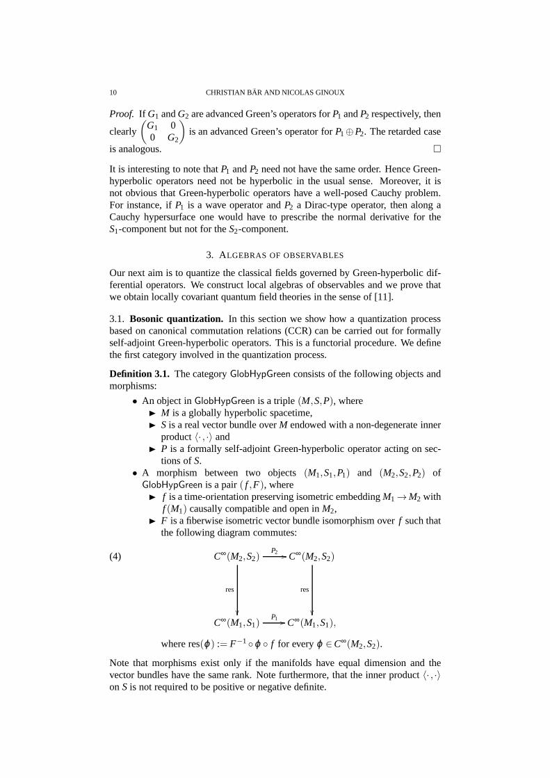
10 CHRISTIAN BAR AND NICOLAS GINOUX
Proof. If G1 andG2 are advanced Green’s operators forP1 andP2 respectively, then
clearly
(G1 00 G2
)is an advanced Green’s operator forP1⊕P2. The retarded case
is analogous.
It is interesting to note thatP1 andP2 need not have the same order. Hence Green-hyperbolic operators need not be hyperbolic in the usual sense. Moreover, it isnot obvious that Green-hyperbolic operators have a well-posed Cauchy problem.For instance, ifP1 is a wave operator andP2 a Dirac-type operator, then along aCauchy hypersurface one would have to prescribe the normal derivative for theS1-component but not for theS2-component.
3. ALGEBRAS OF OBSERVABLES
Our next aim is to quantize the classical fields governed by Green-hyperbolic dif-ferential operators. We construct local algebras of observables and we prove thatwe obtain locally covariant quantum field theories in the sense of [11].
3.1. Bosonic quantization. In this section we show how a quantization processbased on canonical commutation relations (CCR) can be carried out for formallyself-adjoint Green-hyperbolic operators. This is a functorial procedure. We definethe first category involved in the quantization process.
Definition 3.1. The categoryGlobHypGreen consists of the following objects andmorphisms:
• An object inGlobHypGreen is a triple(M,S,P), where M is a globally hyperbolic spacetime, S is a real vector bundle overM endowed with a non-degenerate inner
product〈· , ·〉 and P is a formally self-adjoint Green-hyperbolic operator acting on sec-
tions ofS.• A morphism between two objects(M1,S1,P1) and (M2,S2,P2) ofGlobHypGreen is a pair( f ,F), where f is a time-orientation preserving isometric embeddingM1 →M2 with
f (M1) causally compatible and open inM2, F is a fiberwise isometric vector bundle isomorphism overf such that
the following diagram commutes:
(4) C∞(M2,S2)P2 //
res
C∞(M2,S2)
res
C∞(M1,S1)
P1 // C∞(M1,S1),
where res(ϕ) := F−1ϕ f for everyϕ ∈C∞(M2,S2).
Note that morphisms exist only if the manifolds have equal dimension and thevector bundles have the same rank. Note furthermore, that the inner product〈· , ·〉on S is not required to be positive or negative definite.

CLASSICAL AND QUANTUM FIELDS ON LORENTZIAN MANIFOLDS 11
The causal compatibility condition, which is not automatically satisfied (see e.g.[4, Fig. 33]), ensures the commutation of the extension and restriction maps withthe Green’s operators:
Lemma 3.2. Let ( f ,F) be a morphism between two objects(M1,S1,P1) and(M2,S2,P2) in the categoryGlobHypGreen and let(G1)± and(G2)± be the respec-tive Green’s operators for P1 and P2. Denote byext(ϕ) ∈C∞
c (M2,S2) the extensionby0 of F ϕ f−1 : f (M1)→ S2 to M2, for everyϕ ∈C∞
c (M1,S1). Then
res (G2)± ext= (G1)±.
Proof. Set(G1)± := res (G2)± ext and fixϕ ∈ C∞c (M1,S1). First observe that
the causal compatibility condition onf implies that
supp((G1)±(ϕ)) = f−1(supp((G2)± ext(ϕ)))
⊂ f−1(JM2± (supp(ext(ϕ))))
= f−1(JM2± ( f (supp(ϕ))))
= JM1± (supp(ϕ)).
In particular,(G1)±(ϕ) has spacelike compact support inM1 and(G1)± satisfiesAxiom (G3). Moreover, it follows from (4) thatP2ext= extP1 onC∞
c (M1,S1),which directly implies that(G1)± satisfies Axioms(G1) and (G2) as well. Theuniqueness of the advanced and retarded Green’s operators on M1 yields (G1)± =(G1)±.
Next we show how the Green’s operators for a formally self-adjoint Green-hyperbolic operator provide a symplectic vector space in a canonical way. Firstwe see how the Green’s operators of an operator and of its formally dual operatorare related.
Lemma 3.3. Let M be a globally hyperbolic spacetime and G+,G− the advancedand retarded Green’s operators for a Green-hyperbolic operator P acting on sec-tions of S→ M. Then the advanced and retarded Green’s operators G∗
+ and G∗−
for P∗ satisfy ∫
M〈G∗
±ϕ ,ψ〉dV =∫
M〈ϕ ,G∓ψ〉dV
for all ϕ ∈C∞c (M,S∗) andψ ∈C∞
c (M,S).
Proof. Axiom (G1) for the Green’s operators implies that∫
M〈G∗
±ϕ ,ψ〉dV =
∫
M〈G∗
±ϕ ,P(G∓ψ)〉dV
=∫
M〈P∗(G∗
±ϕ),G∓ψ〉dV
=
∫
M〈ϕ ,G∓ψ〉dV,
where the integration by parts is justified since supp(G∗±ϕ) ∩ supp(G∓ψ) ⊂
JM± (supp(ϕ))∩JM
∓ (supp(ψ)) is compact.
Proposition 3.4. Let (M,S,P) be an object in the categoryGlobHypGreen. SetG := G+−G−, where G+,G− are the advanced and retarded Green’s operator forP, respectively.

12 CHRISTIAN BAR AND NICOLAS GINOUX
Then the pair(SYMPL(M,S,P),ω) is a symplectic vector space, where
SYMPL(M,S,P) :=C∞c (M,S)/ker(G) and ω([ϕ ], [ψ ]) :=
∫
M〈Gϕ ,ψ〉dV.
Here the square brackets[·] denote residue classes moduloker(G).
Proof. The bilinear form(ϕ ,ψ) 7→∫
M〈Gϕ ,ψ〉dV onC∞c (M,S) is skew-symmetric
as a consequence of Lemma 3.3 becauseP is formally self-adjoint. Its null-spaceis exactly ker(G). Therefore the induced bilinear formω on the quotient spaceSYMPL(M,S,P) is non-degenerate and hence a symplectic form.
PutC∞sc(M,S) := ϕ ∈ C∞(M,S) |supp(ϕ) is spacelike compact. The next result
will in particular show that we can consider SYMPL(M,S,P) as the space ofsmooth solutions of the equationPϕ = 0 which have spacelike compact support.
Theorem 3.5. Let M be a Lorentzian manifold, let S→ M be a vector bundle, andlet P be a Green-hyperbolic operator acting on sections of S.Let G± be advancedand retarded Green’s operators for P, respectively. Put
G := G+−G− : C∞c (M,S)→C∞
sc(M,S).
Then the following linear maps form a complex:
(5) 0 →C∞c (M,S)
P−→C∞c (M,S)
G−→C∞sc(M,S)
P−→C∞sc(M,S).
This complex is always exact at the first C∞c (M,S). If M is globally hyperbolic, then
the complex is exact everywhere.
Proof. The proof follows the lines of [4, Thm. 3.4.7] where the result was shownfor wave operators. First note that, by (G±
3 ) in the definition of Green’s operators,we have thatG± : C∞
c (M,S)→C∞sc(M,S). It is clear from (G1) and (G2) thatPG=
GP= 0 onC∞c (M,S), hence (5) is a complex.
If ϕ ∈ C∞c (M,S) satisfiesPϕ = 0, then by (G2) we haveϕ = G+Pϕ = 0 which
shows thatP|C∞c (M,S)
is injective. Thus the complex is exact at the firstC∞c (M,S).
From now on letM be globally hyperbolic. Letϕ ∈C∞c (M,S) with Gϕ = 0, i.e.,
G+ϕ = G−ϕ . We putψ := G+ϕ = G−ϕ ∈C∞(M,S) and we see that supp(ψ) =supp(G+ϕ)∩supp(G−ϕ)⊂ J+(supp(ϕ))∩J−(supp(ϕ)). Since(M,g) is globallyhyperbolicJ+(supp(ϕ))∩ J−(supp(ϕ)) is compact, henceψ ∈ C∞
c (M,S). FromPψ =PG+ϕ =ϕ we see thatϕ ∈P(C∞
c (M,S)). This shows exactness at the secondC∞
c (M,S).It remains to show that anyϕ ∈ C∞
sc(M,S) with Pϕ = 0 is of the formϕ = Gψwith ψ ∈C∞
c (M,S). Using a cut-off function decomposeϕ asϕ = ϕ+−ϕ− wheresupp(ϕ±)⊂ J±(K) whereK is a suitable compact subset ofM. Thenψ := Pϕ+ =Pϕ− satisfies supp(ψ) ⊂ J+(K)∩ J−(K). Thus ψ ∈ C∞
c (M,S). We check thatG+ψ = ϕ+. Namely, for allχ ∈C∞
c (M,S∗) we have by Lemma 3.3∫
M〈χ ,G+Pϕ+〉dV =
∫
M〈G∗
−χ ,Pϕ+〉dV =
∫
M〈P∗G∗
−χ ,ϕ+〉dV =
∫
M〈χ ,ϕ+〉dV.
The integration by parts in the second equality is justified because supp(ϕ+)∩supp(G∗
−χ)⊂ J+(K)∩J−(supp(χ)) is compact. Similarly, one showsG−ψ = ϕ−.Now Gψ = G+ψ −G−ψ = ϕ+−ϕ− = ϕ which concludes the proof.

CLASSICAL AND QUANTUM FIELDS ON LORENTZIAN MANIFOLDS 13
In particular, given an object(M,S,P) in GlobHypGreen, the mapG induces anisomorphism from
SYMPL(M,S,P) =C∞c (M,S)/ker(G)
∼=−→ ker(P)∩C∞sc(M,S).
Remark 3.6. Exactness at the firstC∞c (M,S) in sequence (5) says that there are
no non-trivial smooth solutions ofPϕ = 0 with compact support. Indeed, ifM isglobally hyperbolic, more is true.If ϕ ∈C∞(M,S) solves Pϕ = 0 andsupp(ϕ) is future or past-compact, thenϕ = 0.Here a subsetA⊂M is called future-compact ifA∩J+(x) is compact for anyx∈M.Past-compactness is defined similarly.
Proof. Let ϕ ∈C∞(M,S) solvePϕ = 0 such that supp(ϕ) is future-compact. Foranyχ ∈C∞
c (M,S∗) we have∫
M〈χ ,ϕ〉dV =
∫
M〈P∗G∗
+χ ,ϕ〉dV =
∫
M〈G∗
+χ ,Pϕ〉dV = 0.
This showsϕ = 0. The integration by parts is justified because supp(G∗+χ)∩
supp(ϕ)⊂ J+(supp(χ))∩supp(ϕ) is compact, see [4, Lemma A.5.3].
Remark 3.7. Let M be a globally hyperbolic spacetime and(M,S,P) an object inGlobHypGreen. Then the Green’s operators G+ and G− are unique.Namely, ifG+ andG+ are advanced Green’s operators forP, then for anyϕ ∈C∞
c (M,S) thesectionψ := G+ϕ − G+ϕ has past-compact support and satisfiesPψ = 0. By theprevious remark, we haveψ = 0 which showsG+ = G+.
Now, let( f ,F) be a morphism between two objects(M1,S1,P1) and(M2,S2,P2) inthe categoryGlobHypGreen. For ϕ ∈ C∞
c (M1,S1) consider the extension by zeroext(ϕ) ∈C∞
c (M2,S2) as in Lemma 3.2.
Lemma 3.8. Given a morphism( f ,F) between two objects(M1,S1,P1) and(M2,S2,P2) in the categoryGlobHypGreen, extension by zero induces a symplecticlinear mapSYMPL( f ,F) : SYMPL(M1,S1,P1)→ SYMPL(M2,S2,P2).Moreover,
(6) SYMPL(idM, idS) = idSYMPL(M,S,P)
and for any further morphism( f ′,F ′) : (M2,S2,P2)→ (M3,S3,P3) one has
(7) SYMPL(( f ′,F ′) ( f ,F)) = SYMPL( f ′,F ′)SYMPL( f ,F).
Proof. If ϕ = P1ψ ∈ ker(G1) = P1(C∞c (M1,S1)), then ext(ϕ) = P2(ext(ψ)) ∈
P2(C∞c (M2,S2)) = ker(G2). Hence ext induces a linear map
SYMPL( f ,F) : C∞c (M1,S1)/ker(G1)→C∞
c (M2,S2)/ker(G2).
Furthermore, applying Lemma 3.2, we have, for anyϕ ,ψ ∈C∞c (M1,S1)
∫
M2
〈G2(ext(ϕ)),ext(ψ)〉dV =
∫
M1
〈resG2ext(ϕ),ψ〉dV =
∫
M1
〈G1ϕ ,ψ〉dV,
hence SYMPL( f ,F) is symplectic. Equation (6) is trivial and extending once ortwice by 0 amounts to the same, so (7) holds as well.
Remark 3.9. Under the isomorphism SYMPL(M,S,P) → ker(P)∩C∞sc(M,S) in-
duced byG, the extension by zero corresponds to an extension as a smooth solutionof Pϕ = 0 with spacelike compact support. This follows directly from Lemma 3.2.
14 CHRISTIAN BAR AND NICOLAS GINOUX
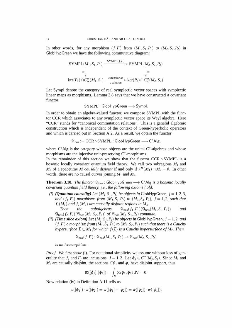
In other words, for any morphism( f ,F) from (M1,S1,P1) to (M2,S2,P2) inGlobHypGreen we have the following commutative diagram:
SYMPL(M1,S1,P1)SYMPL( f ,F)
//
∼=
SYMPL(M2,S2,P2)
∼=
ker(P1)∩C∞sc(M1,S1)
extensionas
asolution// ker(P2)∩C∞
sc(M2,S2).
Let Sympl denote the category of real symplectic vector spaces with symplecticlinear maps as morphisms. Lemma 3.8 says that we have constructed a covariantfunctor
SYMPL :GlobHypGreen−→ Sympl.
In order to obtain an algebra-valued functor, we compose SYMPL with the func-tor CCR which associates to any symplectic vector space its Weyl algebra. Here“CCR” stands for “canonical commutation relations”. This is a general algebraicconstruction which is independent of the context of Green-hyperbolic operatorsand which is carried out in Section A.2. As a result, we obtainthe functor
Abos := CCRSYMPL :GlobHypGreen−→ C∗Alg,
whereC∗Alg is the category whose objects are the unital C∗-algebras and whosemorphisms are the injective unit-preserving C∗-morphisms.In the remainder of this section we show that the functor CCRSYMPL is abosonic locally covariant quantum field theory. We call two subregionsM1 andM2 of a spacetimeM causally disjointif and only if JM(M1)∩M2 = /0. In otherwords, there are no causal curves joiningM1 andM2.
Theorem 3.10. The functorAbos : GlobHypGreen −→ C∗Alg is a bosonic locallycovariant quantum field theory, i.e., the following axioms hold:
(i) (Quantum causality) Let(M j ,Sj ,Pj) be objects inGlobHypGreen, j = 1,2,3,and ( f j ,Fj) morphisms from(M j ,Sj ,Pj) to (M3,S3,P3), j = 1,2, such thatf1(M1) and f2(M2) are causally disjoint regions in M3.
Then the subalgebras Abos( f1,F1)(Abos(M1,S1,P1)) andAbos( f2,F2)(Abos(M2,S2,P2)) of Abos(M3,S3,P3) commute.
(ii) (Time slice axiom) Let(M j ,Sj ,Pj) be objects inGlobHypGreen, j = 1,2, and( f ,F) a morphism from(M1,S1,P1) to (M2,S2,P2) such that there is a CauchyhypersurfaceΣ ⊂ M1 for which f(Σ) is a Cauchy hypersurface of M2. Then
Abos( f ,F) : Abos(M1,S1,P1)→ Abos(M2,S2,P2)
is an isomorphism.
Proof. We first show (i). For notational simplicity we assume without loss of gen-erality that f j andFj are inclusions,j = 1,2. Let ϕ j ∈C∞
c (M j ,Sj). SinceM1 andM2 are causally disjoint, the sectionsGϕ1 andϕ2 have disjoint support, thus
ω([ϕ1], [ϕ2]) =
∫
M〈Gϕ1,ϕ2〉dV = 0.
Now relation (iv) in Definition A.11 tells us
w([ϕ1]) ·w([ϕ2]) = w([ϕ1]+ [ϕ2]) = w([ϕ2]) ·w([ϕ1]).

CLASSICAL AND QUANTUM FIELDS ON LORENTZIAN MANIFOLDS 15
SinceAbos( f1,F1)(Abos(M1,S1,P1)) is generated by elements of the formw([ϕ1])andAbos( f2,F2)(Abos(M2,S2,P2)) by elements of the formw([ϕ2]), the assertionfollows.In order to prove (ii) we show that SYMPL( f ,F) is an isomorphism of symplec-tic vector spaces providedf maps a Cauchy hypersurface ofM1 onto a Cauchyhypersurface ofM2. Since symplectic linear maps are always injective, we onlyneed to show surjectivity of SYMPL( f ,F). This is most easily seen by replacingSYMPL(M j ,Sj ,Pj) by ker(Pj)∩C∞
sc(M j ,Sj) as in Remark 3.9. Again we assumewithout loss of generality thatf andF are inclusions.Let ψ ∈C∞
sc(M2,S2) be a solution ofP2ψ = 0. Letϕ be the restriction ofψ to M1.Thenϕ solvesP1ϕ = 0 and has spacelike compact support inM1 by Lemma 3.11below. We will show that there is only one solution inM2 with spacelike com-pact support extendingϕ . It will then follow that ψ is the image ofϕ under theextension map corresponding to SYMPL( f ,F) and surjectivity will be shown.To prove uniqueness of the extension, we may, by linearity, assume thatϕ = 0.Thenψ+ defined by
ψ+(x) :=
ψ(x), if x∈ JM2
+ (Σ),0, otherwise,
is smooth sinceψ vanishes in an open neighborhood ofΣ. Now ψ+ solvesP2ψ+ =0 and has past-compact support. By Remark 3.6,ψ+ ≡ 0, i.e., ψ vanishes onJM2+ (Σ). One shows similarly thatψ vanishes onJM2
− (Σ), henceψ = 0.
Lemma 3.11. Let M be a globally hyperbolic spacetime and let M′ ⊂ M be acausally compatible open subset which contains a Cauchy hypersurface of M. LetA⊂ M be spacelike compact in M.Then A∩M′ is spacelike compact in M′.
Proof. Fix a common Cauchy hypersurfaceΣ of M′ andM. By assumption, thereexists a compact subsetK ⊂ M with A⊂ JM(K). ThenK′ := JM(K)∩Σ is compact[4, Cor. A.5.4] and contained inM′.MoreoverA⊂ JM(K′): let p∈ A and letγ be a causal curve (inM) from p to somek∈ K. Thenγ can be extended to an inextensible causal curve inM, which hencemeetsΣ at some pointq. Because ofq∈ Σ∩JM(k)⊂ K′ one hasp∈ JM(K′).ThereforeA∩M′ ⊂ JM(K′)∩M′ = JM′
(K′) because of the causal compatibility ofM′ in M. The lemma is proved.
The quantization process described in this subsection applies in particular to for-mally self-adjoint wave and Dirac-type operators.
3.2. Fermionic quantization. Next we construct a fermionic quantization. Forthis we need a functorial construction of Hilbert spaces rather than symplecticvector spaces. As we shall see this seems to be possible only under much morerestrictive assumptions. The underlying Lorentzian manifold M is assumed to bea globally hyperbolic spacetime as before. The vector bundle S is assumed to becomplex with Hermitian inner product〈· , ·〉 which may be indefinite. The formallyself-adjoint Green-hyperbolic operatorP is assumed to be of first order.
Definition 3.12. A formally self-adjoint Green-hyperbolic operatorP of first orderacting on sections of a complex vector bundleSover a spacetimeM is of definite

16 CHRISTIAN BAR AND NICOLAS GINOUX
type if and only if for anyx ∈ M and any future-directed timelike tangent vectorn ∈ TxM, the bilinear map
Sx×Sx → C, (ϕ ,ψ) 7→ 〈iσP(n) ·ϕ ,ψ〉,
yields a positive definite Hermitian scalar product onSx.
Example 3.13.The classical Dirac operatorP from Example 2.21 is, when definedwith the correct sign, of definite type, see e.g. [5, Sec. 1.1.5] or [3, Sec. 2].
Example 3.14. If E → M is a semi-Riemannian or -Hermitian vector bundle en-dowed with a metric connection over a spin spacetimeM, then the twisted Diracoperator from Example 2.22 is of definite type if and only if the metric onE ispositive definite. This can be seen by evaluating the tensorized inner product onelements of the formσ ⊗v, wherev∈ Ex is null.
Example 3.15. The operatorP= i(d−δ ) on S= ΛT∗M⊗C is of Dirac type butnot of definite type. This follows from Example 3.14 applied to Example 2.23,since the natural inner product onΣM is not positive definite. An alternative el-ementary proof is the following: for any timelike tangent vector n on M and thecorresponding covectorn, one has
〈iσP(n)n,n〉=−〈n∧n
−nyn,n〉= 〈n,n〉〈1,n〉= 0.
Example 3.16. The Rarita-Schwinger operator defined in Section 2.6 is not ofdefinite type if the dimension of the manifolds ism≥ 3. This can be seen asfollows. Fix a pointx ∈ M and a pointwise orthonormal basis(ej)1≤ j≤m of TxMwith e1 timelike. The Lorentzian metric induces inner products onΣM and onΣ3/2M which we denote by〈· , ·〉. Chooseξ := e1 ∈ T∗
x M andψ ∈ Σ3/2x M. Since
σQ(ξ ) is pointwise obtained as the orthogonal projection ofσD(ξ ) onto Σ3/2x M,
one has
〈−iσQ(ξ )ψ ,ψ〉 = 〈(id⊗ξ ♯·)ψ ,ψ〉− 2m
m
∑β=1
〈e∗β ⊗eβ ·ψ1,ψ〉︸ ︷︷ ︸
=0
=m
∑β=1
εβ 〈e1 ·ψβ ,ψβ 〉.
Choose, as in the proof of Lemma 2.26, aψ ∈ Σ3/2x M with ψk = 0 for all 3≤ k≤m.
For such aψ the conditionψ ∈ Σ3/2x M becomese1 ·ψ1 = e2 ·ψ2. As in the proof
of Lemma 2.26 we obtain
〈−iσQ(ξ )ψ ,ψ〉=−〈e1 ·ψ2,ψ2〉+ 〈e1 ·ψ2,ψ2〉= 0,
which shows that the Rarita-Schwinger operator cannot be ofdefinite type.
We define the categoryGlobHypDef, whose objects are the triples(M,S,P), whereM is a globally hyperbolic spacetime,S is a complex vector bundle equipped witha complex inner product〈· , ·〉, andP is a formally self-adjoint Green-hyperbolicoperator of definite type acting on sections ofS. The morphisms are the same as inthe categoryGlobHypGreen.We construct a covariant functor fromGlobHypDef to HILB, whereHILB denotesthe category whose objects are complex pre-Hilbert spaces and whose morphismsare isometric linear embeddings. As in Section 3.1, the underlying vector space

CLASSICAL AND QUANTUM FIELDS ON LORENTZIAN MANIFOLDS 17
is the space of classical solutions to the equationPϕ = 0 with spacelike compactsupport. We put
SOL(M,S,P) := ker(P)∩C∞sc(M,S).
Here “SOL” stands for classical solutions of the equationPϕ = 0 with spacelikecompact support.
Lemma 3.17. Let (M,S,P) be an object inGlobHypDef. Let Σ ⊂ M be a smoothspacelike Cauchy hypersurface with its future-oriented unit normal vector fieldnand its induced volume elementdA. Then
(8) (ϕ ,ψ) :=∫
Σ〈iσP(n
) ·ϕ|Σ ,ψ|Σ〉dA,
yields a positive definite Hermitian scalar product onSOL(M,S,P) which does notdepend on the choice ofΣ.
Proof. First note that supp(ϕ)∩Σ is compact since supp(ϕ) is spacelike compact,so that the integral is well-defined. We have to show that it does not depend onthe choice of Cauchy hypersurface. LetΣ′ be any other smooth spacelike Cauchyhypersurface. Assume first thatΣ and Σ′ are disjoint and letΩ be the domainenclosed byΣ andΣ′ in M. Its boundary is∂Ω = Σ∪Σ′. Without loss of generality,one may assume thatΣ′ ⊂ JM
+ (Σ). By the Green’s formula [40, p. 160, Prop. 9.1]we have for allϕ ,ψ ∈C∞
sc(M,S),
(9)∫
Ω(〈Pϕ ,ψ〉− 〈ϕ ,Pψ〉) dV =
∫
Σ′〈σP(n
)ϕ ,ψ〉dA−∫
Σ〈σP(n
)ϕ ,ψ〉dA.
For ϕ ,ψ ∈ SOL(M,S,P) we havePϕ = Pψ = 0 and thus
0=∫
Σ〈σP(n
)ϕ ,ψ〉dA−∫
Σ′〈σP(n
)ϕ ,ψ〉dA.
This shows the result in the caseΣ∩Σ′ = /0.If Σ∩Σ′ 6= /0 consider the subsetIM
− (Σ)∩ IM− (Σ′) of M where, as usual,IM
+ (Σ) andIM− (Σ) denote the chronological future and past of the subsetΣ in M, respectively.
This subset is nonempty, open, and globally hyperbolic. This follows e.g. from[4, Lemma A.5.8]. Hence it admits a smooth spacelike Cauchy hypersurfaceΣ′′
by Theorem 2.3. By construction,Σ′′ meets neitherΣ nor Σ′ and it can be easilychecked thatΣ′′ is also a Cauchy hypersurface ofM. The result follows from theargument above being applied first to the pair(Σ,Σ′′) and then to the pair(Σ′′,Σ′).
Remark 3.18. If one drops the assumption thatP be of definite type, then theabove sesquilinear form(· , ·) on ker(P)∩C∞
sc(M,S) still does not depend on thechoice ofΣ, however it need no longer be positive definite and can even bede-generate. Pick for instance the spin Dirac operatorDg associated to the underlyingLorentzian metricg on a spin spacetimeM (see Example 2.21) and, keeping thespinor bundleΣgM associated tog, change the metric onM so that the new met-ric g′ has larger future and past cones at each point. Note that thisimplies thatany globally hyperbolic subregion of(M,g′) is also globally hyperbolic in(M,g).Then, denoting byD∗
g the formal adjoint ofDg with respect to the metricg′, the
operator
(0 Dg
D∗g 0
)on ΣgM⊕ΣgM remains Green-hyperbolic but it fails to be
of definite type, since there exist timelike vectors forg′ which are lightlike forg.

18 CHRISTIAN BAR AND NICOLAS GINOUX
Hence the principal symbol of the operator becomes non-invertible and the bilinearform in (8) becomes degenerate for theseg′-timelike covectors.
For any object(M,S,P) in GlobHypDef we will from now on equip SOL(M,S,P)with the Hermitian scalar product in (8) and thus turn SOL(M,S,P) into a pre-Hilbert space.Given a morphism( f ,F) from (M1,S1,P1) to (M2,S2,P2) in GlobHypDef, thenthis is also a morphism inGlobHypGreen and hence induces a homomor-phism SYMPL( f ,F) : SYMPL(M1,S1,P1) → SYMPL(M2,S2,P2). As explainedin Remark 3.9, there is a corresponding extension homomorphism SOL( f ,F) :SOL(M1,S1,P1) → SOL(M2,S2,P2). In other words, SOL( f ,F) is defined suchthat the diagram
(10) SYMPL(M1,S1,P1)SYMPL( f ,F)
//
∼=
SYMPL(M2,S2,P2)
∼=
SOL(M1,S1,P1)SOL( f ,F)
// SOL(M2,S2,P2)
commutes. The vertical arrows are the vector space isomorphisms induced be theGreen’s propagatorsG1 andG2, respectively.
Lemma 3.19. The vector space homomorphismSOL( f ,F) : SOL(M1,S1,P1) →SOL(M2,S2,P2) preserves the scalar products, i.e., it is an isometric linear embed-ding of pre-Hilbert spaces.
Proof. Without loss of generality we assume thatf andF are inclusions. LetΣ1
be a spacelike Cauchy hypersurface ofM1. Let ϕ1,ψ1 ∈C∞sc(M1,S1). Denote the
extension ofϕ1 by ϕ2 := SOL( f ,F)(ϕ1) and similarly forψ1.Let K1 ⊂ M1 be a compact subset such that supp(ϕ2) ⊂ JM2(K1) and supp(ψ2) ⊂JM2(K1). We choose a compact submanifoldK ⊂ Σ1 with boundary such thatJM1(K1) ∩ Σ1 ⊂ K. Since Σ1 is a Cauchy hypersurface inM1, JM1(K1) ⊂JM1(JM1(K1)∩Σ1)⊂ JM1(K).By Theorem 2.5 there is a spacelike Cauchy hypersurfaceΣ2 ⊂ M2 containingK. SinceΣi is a Cauchy hypersurface ofMi (where i = 1,2), it is met by everyinextensible causal curve [30, Lemma 14.29]. Moreover, by definition of a Cauchyhypersurface,Σi is achronal inMi. Since it is also spacelike,Σi is even acausal [30,Lemma 14.42]. In particular, it is metexactly onceby every inextensible causalcurve inMi.This impliesJM2(K1) ⊂ JM2(K): namely, pickp ∈ JM2(K1) and a causal curveγin M2 from p to somek1 ∈ K1. Extendγ to an inextensible causal curveγ in M2.Thenγ meetsΣ2 at some pointq2, becauseΣ2 is a Cauchy hypersurface inM2. Butγ ∩M1 is also an inextensible causal curve inM1, hence it intersectsΣ1 at a pointq1, which must lie inK by definition ofK. Because ofK ⊂ Σ2 and the uniquenessof the intersection point, one hasq1 = q2. In particular,p∈ JM2(K).

CLASSICAL AND QUANTUM FIELDS ON LORENTZIAN MANIFOLDS 19
M2
K1M1
JM2(K1)
Σ2
Σ1K
Fig. 1
We conclude supp(ϕ2) ⊂ JM2(K). Since K ⊂ Σ2, we have supp(ϕ2) ∩ Σ2 ⊂JM2(K) ∩ Σ2 and JM2(K) ∩ Σ2 = K using the acausality ofΣ2. This showssupp(ϕ2)∩Σ2 = supp(ϕ1)∩Σ1 and similarly forψ2. Now we get
(ϕ2,ψ2) =
∫
Σ2
〈iσP2(n) ·ϕ2,ψ2〉dA =
∫
Σ1
〈iσP1(n) ·ϕ1,ψ1〉dA = (ϕ1,ψ1)
and the lemma is proved.
The functoriality of SYMPL and diagram (10) show that SOL is afunctor fromGlobHypDef to HILB, the category of complex pre-Hilbert spaces with isometriclinear embeddings. Composing with the functor CAR (see Section A.1), we obtainthe covariant functor
Aferm := CARSOL :GlobHypDef −→ C∗Alg.
The fermionic algebrasAferm(M,S,P) are actuallyZ2-graded algebras, see Propo-sition A.5 (iii).
Theorem 3.20.The functorAferm : GlobHypDef −→ C∗Alg is a fermionic locallycovariant quantum field theory, i.e., the following axioms hold:
(i) (Quantum causality) Let (M j ,Sj ,Pj) be objects inGlobHypDef, j = 1,2,3,and ( f j ,Fj) morphisms from(M j ,Sj ,Pj) to (M3,S3,P3), j = 1,2, such thatf1(M1) and f2(M2) are causally disjoint regions in M3.Then the subalgebras Aferm( f1,F1)(Aferm(M1,S1,P1)) andAferm( f2,F2)(Aferm(M2,S2,P2)) of Aferm(M3,S3,P3) super-commute1.
(ii) (Time slice axiom) Let (M j ,Sj ,Pj) be objects inGlobHypDef, j = 1,2, and( f ,F) a morphism from(M1,S1,P1) to (M2,S2,P2) such that there is a CauchyhypersurfaceΣ ⊂ M1 for which f(Σ) is a Cauchy hypersurface of M2. Then
Aferm( f ,F) : Aferm(M1,S1,P1)→ Aferm(M2,S2,P2)
is an isomorphism.
1This means that the odd parts of the algebras anti-commute while the even parts commute witheverything.
20 CHRISTIAN BAR AND NICOLAS GINOUX
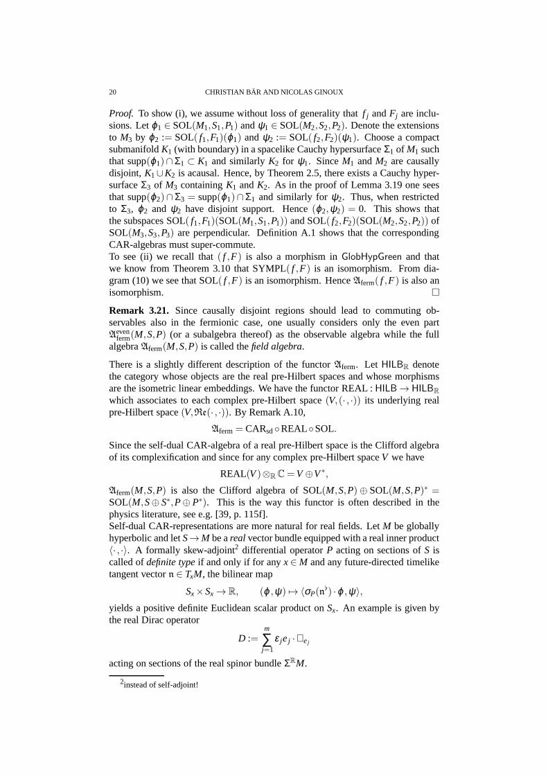
Proof. To show (i), we assume without loss of generality thatf j andFj are inclu-sions. Letϕ1 ∈ SOL(M1,S1,P1) andψ1 ∈ SOL(M2,S2,P2). Denote the extensionsto M3 by ϕ2 := SOL( f1,F1)(ϕ1) andψ2 := SOL( f2,F2)(ψ1). Choose a compactsubmanifoldK1 (with boundary) in a spacelike Cauchy hypersurfaceΣ1 of M1 suchthat supp(ϕ1)∩Σ1 ⊂ K1 and similarlyK2 for ψ1. SinceM1 andM2 are causallydisjoint, K1∪K2 is acausal. Hence, by Theorem 2.5, there exists a Cauchy hyper-surfaceΣ3 of M3 containingK1 andK2. As in the proof of Lemma 3.19 one seesthat supp(ϕ2)∩Σ3 = supp(ϕ1)∩Σ1 and similarly forψ2. Thus, when restrictedto Σ3, ϕ2 and ψ2 have disjoint support. Hence(ϕ2,ψ2) = 0. This shows thatthe subspaces SOL( f1,F1)(SOL(M1,S1,P1)) and SOL( f2,F2)(SOL(M2,S2,P2)) ofSOL(M3,S3,P3) are perpendicular. Definition A.1 shows that the correspondingCAR-algebras must super-commute.To see (ii) we recall that( f ,F) is also a morphism inGlobHypGreen and thatwe know from Theorem 3.10 that SYMPL( f ,F) is an isomorphism. From dia-gram (10) we see that SOL( f ,F) is an isomorphism. HenceAferm( f ,F) is also anisomorphism.
Remark 3.21. Since causally disjoint regions should lead to commuting ob-servables also in the fermionic case, one usually considersonly the even partAeven
ferm(M,S,P) (or a subalgebra thereof) as the observable algebra while the fullalgebraAferm(M,S,P) is called thefield algebra.
There is a slightly different description of the functorAferm. Let HILBR denotethe category whose objects are the real pre-Hilbert spaces and whose morphismsare the isometric linear embeddings. We have the functor REAL : HILB→ HILBR
which associates to each complex pre-Hilbert space(V,(· , ·)) its underlying realpre-Hilbert space(V,Re(· , ·)). By Remark A.10,
Aferm = CARsdREALSOL.
Since the self-dual CAR-algebra of a real pre-Hilbert spaceis the Clifford algebraof its complexification and since for any complex pre-Hilbert spaceV we have
REAL(V)⊗RC=V ⊕V∗,
Aferm(M,S,P) is also the Clifford algebra of SOL(M,S,P)⊕ SOL(M,S,P)∗ =SOL(M,S⊕ S∗,P⊕ P∗). This is the way this functor is often described in thephysics literature, see e.g. [39, p. 115f].Self-dual CAR-representations are more natural for real fields. LetM be globallyhyperbolic and letS→M be areal vector bundle equipped with a real inner product〈· , ·〉. A formally skew-adjoint2 differential operatorP acting on sections ofS iscalled ofdefinite typeif and only if for anyx∈ M and any future-directed timeliketangent vectorn ∈ TxM, the bilinear map
Sx×Sx → R, (ϕ ,ψ) 7→ 〈σP(n) ·ϕ ,ψ〉,
yields a positive definite Euclidean scalar product onSx. An example is given bythe real Dirac operator
D :=m
∑j=1
ε jej ·∇ej
acting on sections of the real spinor bundleΣRM.
2instead of self-adjoint!

CLASSICAL AND QUANTUM FIELDS ON LORENTZIAN MANIFOLDS 21
Given a smooth spacelike Cauchy hypersurfaceΣ ⊂ M with future-directed time-like unit normal fieldn, we define a scalar product on SOL(M,S,P) = ker(P)∩C∞
sc(M,S,P) by
(ϕ ,ψ) :=∫
Σ〈σP(n
) ·ϕ|Σ,ψ|Σ〉dA.
With essentially the same proofs as before, one sees that this scalar productdoes not depend on the choice of Cauchy hypersurfaceΣ and that a morphism( f ,F) : (M1,S1,P1)→ (M2,S2,P2) gives rise to an extension operator SOL( f ,F) :SOL(M1,S1,P1) → SOL(M2,S2,P2) preserving the scalar product. We have con-structed a functor
SOL :GlobHypSkewDef −→ HILBR
whereGlobHypSkewDef denotes the category whose objects are triples(M,S,P)with M globally hyperbolic,S→ M a real vector bundle with real inner productandP a formally skew-adjoint, Green-hyperbolic differential operator of definitetype acting on sections ofS. The morphisms are the same as before.Now the functor
Asdferm := CARsdSOL :GlobHypSkewDef −→ C∗Alg
is a locally covariant quantum field theory in the sense that Theorem 3.20 holdswith Aferm replaced byAsd
ferm.
4. STATES AND QUANTUM FIELDS
In order to produce numbers out of our quantum field theory that can be comparedto experiments, we need states, in addition to observables.We briefly recall therelation between states and representations via the GNS-construction. Then weshow how the choice of a state gives rise to quantum fields andn-point functions.
4.1. States and representations.Recall that astateon a unital C∗-algebraA is alinear functionalτ : A→ C such that
(i) τ is positive, i.e.,τ(a∗a)≥ 0 for all a∈ A;(ii) τ is normed, i.e.,τ(1) = 1.
One checks that for any state the sesquilinear formA×A→ C, (a,b) 7→ τ(b∗a),is a positive semi-definite Hermitian product and|τ(a)| ≤ ‖a‖ for all a ∈ A. Inparticular,τ is continuous.Any state induces a representation ofA. Namely, the sesquilinear formτ(b∗a)induces a scalar product〈·, ·〉τ onA/a∈ A | τ(a∗a) = 0. The Hilbert space com-pletion of A/a ∈ A | τ(a∗a) = 0 is denoted byHτ . The action ofA on Hτ isinduced by the multiplication inA,
πτ(a)[b]τ := [ab]τ ,
where [a]τ denotes the residue class ofa ∈ A in A/a ∈ A | τ(a∗a) = 0. Thisrepresentation is known as theGNS-representationinduced byτ . The residue classΩτ := [1]τ ∈ Hτ is called thevacuum vector. By construction, it is a cyclic vector,i.e., the orbitπτ(A) ·Ωτ = A/a∈ A | τ(a∗a) = 0 is dense inHτ .The GNS-representation together with the vacuum vector allows to reconstruct thestate since
(11) τ(a) = τ(1∗a1) = 〈πτ(a)Ωτ ,Ωτ〉τ .
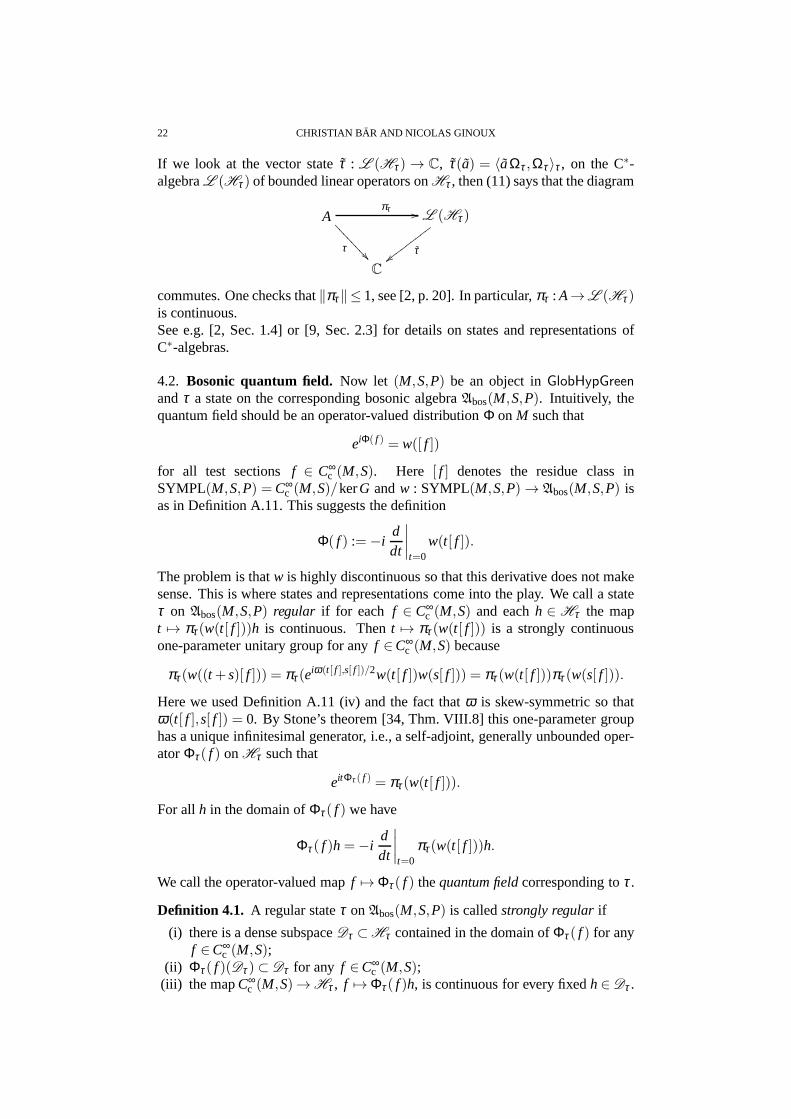
22 CHRISTIAN BAR AND NICOLAS GINOUX
If we look at the vector stateτ : L (Hτ) → C, τ(a) = 〈aΩτ ,Ωτ〉τ , on the C∗-algebraL (Hτ) of bounded linear operators onHτ , then (11) says that the diagram
Aπτ //
τ=
====
===
L (Hτ)
τww
wwww
www
C
commutes. One checks that‖πτ‖≤ 1, see [2, p. 20]. In particular,πτ : A→L (Hτ)is continuous.See e.g. [2, Sec. 1.4] or [9, Sec. 2.3] for details on states and representations ofC∗-algebras.
4.2. Bosonic quantum field. Now let (M,S,P) be an object inGlobHypGreenandτ a state on the corresponding bosonic algebraAbos(M,S,P). Intuitively, thequantum field should be an operator-valued distributionΦ on M such that
eiΦ( f ) = w([ f ])
for all test sections f ∈ C∞c (M,S). Here [ f ] denotes the residue class in
SYMPL(M,S,P) = C∞c (M,S)/kerG andw : SYMPL(M,S,P) → Abos(M,S,P) is
as in Definition A.11. This suggests the definition
Φ( f ) := −iddt
∣∣∣∣t=0
w(t[ f ]).
The problem is thatw is highly discontinuous so that this derivative does not makesense. This is where states and representations come into the play. We call a stateτ on Abos(M,S,P) regular if for each f ∈ C∞
c (M,S) and eachh ∈ Hτ the mapt 7→ πτ(w(t[ f ]))h is continuous. Thent 7→ πτ(w(t[ f ])) is a strongly continuousone-parameter unitary group for anyf ∈C∞
c (M,S) because
πτ(w((t +s)[ f ])) = πτ(eiω(t[ f ],s[ f ])/2w(t[ f ])w(s[ f ])) = πτ(w(t[ f ]))πτ (w(s[ f ])).
Here we used Definition A.11 (iv) and the fact thatω is skew-symmetric so thatω(t[ f ],s[ f ]) = 0. By Stone’s theorem [34, Thm. VIII.8] this one-parameter grouphas a unique infinitesimal generator, i.e., a self-adjoint,generally unbounded oper-atorΦτ( f ) onHτ such that
eitΦτ ( f ) = πτ(w(t[ f ])).
For allh in the domain ofΦτ( f ) we have
Φτ( f )h=−iddt
∣∣∣∣t=0
πτ(w(t[ f ]))h.
We call the operator-valued mapf 7→ Φτ( f ) thequantum fieldcorresponding toτ .
Definition 4.1. A regular stateτ onAbos(M,S,P) is calledstrongly regularif
(i) there is a dense subspaceDτ ⊂Hτ contained in the domain ofΦτ( f ) for anyf ∈C∞
c (M,S);(ii) Φτ( f )(Dτ )⊂ Dτ for any f ∈C∞
c (M,S);(iii) the mapC∞
c (M,S)→ Hτ , f 7→ Φτ( f )h, is continuous for every fixedh∈ Dτ .

CLASSICAL AND QUANTUM FIELDS ON LORENTZIAN MANIFOLDS 23
For a strongly regular stateτ we have for allf ,g∈C∞c (M,S), α ,β ∈R andh∈Dτ :
Φτ(α f +βg)h=−iddt
∣∣∣∣t=0
πτ(w(t[α f +βg]))h
=−iddt
∣∣∣∣t=0
eiαβt2ω([ f ],[g])/2πτ(w(αt[ f ]))πτ (w(β t[g]))h
=−iddt
∣∣∣∣t=0
πτ(w(αt[ f ]))h− iddt
∣∣∣∣t=0
πτ(w(β t[g]))h
= αΦτ( f )h+βΦτ(g)h.
HenceΦτ( f ) depends linearly onf . The quantum fieldΦτ is therefore a distribu-tion onM with values in self-adjoint operators onHτ .Then-point functionsare defined by
τn( f1, . . . , fn) := 〈Φτ( f1) · · ·Φτ( fn)Ωτ ,Ωτ〉τ
= τ (Φτ( f1) · · ·Φτ( fn))
= τ
((−i
ddt1
∣∣∣∣t1=0
πτ(w(t1[ f1]))
)· · ·(−i
ddtn
∣∣∣∣tn=0
πτ(w(tn[ fn]))
))
= (−i)n ∂ n
∂ t1 · · ·∂ tn
∣∣∣∣t1=···=tn=0
τ (πτ(w(t1[ f1])) · · ·πτ(w(tn[ fn])))
= (−i)n ∂ n
∂ t1 · · ·∂ tn
∣∣∣∣t1=···=tn=0
τ (πτ(w(t1[ f1]) · · ·w(tn[ fn])))
= (−i)n ∂ n
∂ t1 · · ·∂ tn
∣∣∣∣t1=···=tn=0
τ (w(t1[ f1]) · · ·w(tn[ fn])) .
For a strongly regular stateτ the n-point functions are continuous separately ineach factor. By the Schwartz kernel theorem [23, Thm. 5.2.1]then-point functionτn extends uniquely to a distribution onM × ·· · ×M (n times) in the followingsense: LetS∗⊠ · · ·⊠S∗ be the bundle overM×·· ·×M whose fiber over(x1, . . . ,xn)is given byS∗x1
⊗·· ·⊗S∗xn. Then there is a unique distribution onM×·· ·×M in the
bundleS∗⊠ · · ·⊠S∗, again denotedτn, such that for allf j ∈C∞c (M,S),
τn( f1, . . . , fn) = τn( f1⊗·· ·⊗ fn)
where( f1⊗·· ·⊗ fn)(x1, . . . ,xn) := f1(x1)⊗·· ·⊗ fn(xn).
Theorem 4.2.Let(M,S,P) be an object inGlobHypGreen andτ a strongly regularstate on the corresponding bosonic algebraAbos(M,S,P). Then
(i) PΦτ = 0 and Pτn( f1, . . . , f j−1, ·, f j+1, . . . , fn) = 0 hold in the distributionalsense where fk ∈C∞
c (M,S), k 6= j, are fixed;(ii) the quantum field satisfies the canonical commutation relations, i.e.,
[Φτ( f ),Φτ (g)]h= i∫
M〈G f,g〉dV ·h
for all f ,g∈C∞c (M,S) and h∈ Dτ ;

24 CHRISTIAN BAR AND NICOLAS GINOUX
(iii) the n-point functions satisfy the canonical commutation relations, i.e.,
τn+2( f1, . . . , f j−1, f j , f j+1, . . . , fn+2)
− τn+2( f1, . . . , f j−1, f j+1, f j , f j+2, . . . , fn+2)
= i∫
M〈G f j , f j+1〉dV · τn( f1, . . . , f j−1, f j+2, . . . , fn+2)
for all f1, . . . , fn+2 ∈C∞c (M,S).
Proof. SinceP is formally self-adjoint andGP f= 0 for any f ∈C∞c (M,S), we have
for anyh∈ Dτ :
(PΦτ)( f )h= Φτ(P f)h=−iddt
∣∣∣∣t=0
πτ(w(t [P f ]︸︷︷︸=0
))h=−iddt
∣∣∣∣t=0
h= 0.
This showsPΦτ = 0. The result for then-point functions follows and (i) is proved.To show (ii) we observe that by Definition A.11 (iv) we have on the one hand
w([ f +g]) = eiω([ f ],[g])/2w([ f ])w([g])
and on the other hand
w([ f +g]) = eiω([g],[ f ])/2w([g])w([ f ]),
hence
w([ f ])w([g]) = e−iω([ f ],[g])w([g])w([ f ]).
Thus
Φτ( f )Φτ (g)h=− ∂ 2
∂ t∂s
∣∣∣∣t=s=0
πτ(w(t[ f ])w(s[g]))h
=− ∂ 2
∂ t∂s
∣∣∣∣t=s=0
πτ(e−iω(t[ f ],s[g])w(s[g])w(t[ f ]))h
=− ∂ 2
∂ t∂s
∣∣∣∣t=s=0
e−iω(t[ f ],s[g]) ·πτ(w(s[g])w(t[ f ]))h
= iω([ f ], [g])h+Φτ (g)Φτ ( f )h
= i∫
M〈G f,g〉dV ·h+Φτ(g)Φτ ( f )h.
This shows (ii). Assertion (iii) follows from (ii).
Remark 4.3. As a consequence of the canonical commutation relations we get
[Φτ( f ),Φτ (g)] = 0
if the supports off andg are causally disjoint, i.e., if there is no causal curve fromsupp( f ) to supp(g). The reason is that in this case the supports ofG f andg aredisjoint. A similar remark holds for then-point functions.
Remark 4.4. In the physics literature one also finds the statementΦ( f ) = Φ( f )∗.This simply expresses the fact that we are dealing with a theory over the reals. Wehave encoded this by considering real vector bundlesS, see Definition 3.1, and thefact thatΦτ( f ) is always self-adjoint.

CLASSICAL AND QUANTUM FIELDS ON LORENTZIAN MANIFOLDS 25
4.3. Fermionic quantum fields. Let (M,S,P) be an object inGlobHypDef andlet τ be a state on the fermionic algebraAferm(M,S,P). For f ∈C∞
c (M,S) we put
Φτ( f ) := −πτ(a(G f)∗),
Φ+τ ( f ) := πτ(a(G f)),
wherea is as in Definition A.1 (compare [18, Sec. III.B, p. 141]). Sinceπτ , a, andG are sequentially continuous (forG see [4, Prop. 3.4.8]), so areΦτ andΦ+
τ . Incontrast to the bosonic case, no regularity assumption onτ is needed. HenceΦτandΦ+
τ are distributions onM with values in the space of bounded operators onHτ . Note thatΦτ is linear whileΦ+
τ is anti-linear.
Theorem 4.5. Let (M,S,P) be an object inGlobHypDef and τ a state on thecorresponding fermionic algebraAferm(M,S,P). Then
(i) PΦτ = PΦ+τ = 0 holds in the distributional sense;
(ii) the quantum fields satisfy the canonical anti-commutation relations, i.e.,
Φτ ( f ),Φτ (g) = Φ+τ ( f ),Φ+
τ (g) = 0,
Φτ( f ),Φ+τ (g) = i
(∫
M〈G f,g〉dV
)· idHτ
for all f ,g∈C∞c (M,S).
Proof. SinceGP= 0 onC∞c (M,S), we havePΦτ( f )=Φτ (P f)=−πτ(a(GP f)∗)=
0 and similarly forΦ+τ . This proves assertion (i).
Using Definition A.1 (ii) we compute
Φτ ( f ),Φτ (g)= πτ(a(G f)∗),πτ(a(Gg)∗)= πτ(a(G f)∗,a(Gg)∗)= πτ(a(Gg),a(G f)∗)= 0.
Similarly one seesΦ+τ ( f ),Φ+
τ (g) = 0. Definition A.1 (iii) also yields
Φτ ( f ),Φ+τ (g) =−πτ(a(G f)∗,a(Gg)) =−(G f,Gg) · idHτ .
To prove assertion (ii) we have to verify
(12) (G f,Gg) =−i∫
M〈G f,g〉dV
Let Σ ⊂ M be a smooth spacelike Cauchy hypersurface. Since supp(G+g) is past-compact, we can find a Cauchy hypersurfaceΣ′ ⊂ M in the past ofΣ which doesnot intersect supp(G+g) ⊂ JM
+ (supp(g)). Denote the region betweenΣ andΣ′ byΩ′. The Green’s formula (9) yields
(G f,G+g) =∫
Σ〈iσP(n
) ·G f,G+g〉dA
=
∫
Σ′〈iσP(n
) ·G f,G+g〉dA+ i∫
Ω′(〈PG f,G+g〉− 〈G f,PG+g〉)dV
=−i∫
Ω′〈G f,g〉dV
becausePG+g = g andPG f = 0. SinceΣ′ can be chosen arbitrarily to the past,this shows
(13) (G f,G+g) =−i∫
J−(Σ)〈G f,g〉dV.

26 CHRISTIAN BAR AND NICOLAS GINOUX
A similar computation yields
(14) (G f,G−g) = i∫
J+(Σ)〈G f,g〉dV.
Subtracting (14) from (13) yields (12) and concludes the proof of assertion (ii).
Remark 4.6. Similarly to the bosonic case, we find
Φτ ( f ),Φ+τ (g)= 0
if the supports off andg are causally disjoint.
Remark 4.7. Using the anti-commutation relations in Theorem 4.5 (ii), the com-putation ofn-point functions can be reduced to those of the form
τn,n′( f1, . . . , fn,g1, . . . ,gn′) = 〈Ωτ ,Φτ( f1) · · ·Φτ( fn)Φ+τ (g1) · · ·Φ+
τ (gn′)Ωτ〉τ .
As in the bosonic case, then-point functions satisfy the field equation in the distri-butional sense in each argument and extend to distributionson M×·· ·×M.
If one uses the self-dual fermionic algebraAsdferm(M,S,P) instead ofAferm(M,S,P),
then one gets the quantum field
Ψτ( f ) := πτ(b(G f))
whereb is as in Definition A.6. Then the analogue to Theorem 4.5 is
Theorem 4.8. Let (M,S,P) be an object inGlobHypSkewDef andτ a state on thecorresponding self-dual fermionic algebraAsd
ferm(M,S,P). Then
(i) PΨτ = 0 holds in the distributional sense;(ii) the quantum field takes values in self-adjoint operators, Ψτ( f ) = Ψτ( f )∗ for
all f ∈C∞c (M,S);
(iii) the quantum fields satisfy the canonical anti-commutation relations, i.e.,
Ψτ( f ),Ψτ (g)=∫
M〈G f,g〉dV · idHτ
for all f ,g∈C∞c (M,S).
Remark 4.9. It is interesting to compare the concept of locally covariant quantumfield theories as proposed in [11] to the axiomatic approach to quantum field theoryon Minkowski space based on the Garding-Wightman axioms asexposed in [35,Sec. IX.8]. Property 1 (relativistic invariance of states)and Property 6 (Poincareinvariance of the field) in [35] are replaced by functoriality (covariance). Prop-erty 4 (invariant domain for fields) and Property 5 (regularity of the field) havebeen encoded in strong regularity of the state used to define the quantum field inthe bosonic case and are automatic in the fermionic case. Property 7 (local commu-tativity or microscopic causality) is contained in Theorems 4.2 and 4.5. Property 3(existence and uniqueness of the vacuum) has no analogue andis replaced by thechoiceof a state. Property 8 (cyclicity of the vacuum) is then automatic by thegeneral properties of the GNS-construction.There remains one axiom, Property 2 (spectral condition), which we have not dis-cussed at all. It gets replaced by the Hadamard condition on the state chosen. It wasobserved by Radzikowski [32] that earlier formulations of this condition are equiv-alent to a condition on the wave front set of the 2-point function. Much work hasbeen put into constructing and investigating Hadamard states for various examplesof fields, see e.g. [15, 16, 19, 25, 36, 37, 38, 42] and the references therein.

CLASSICAL AND QUANTUM FIELDS ON LORENTZIAN MANIFOLDS 27
APPENDIX A. A LGEBRAS OF CANONICAL (ANTI -) COMMUTATION
RELATIONS
We collect the necessary algebraic facts about CAR and CCR-algebras.
A.1. CAR algebras. The symbol “CAR” stands for “canonical anti-commutationrelations”. These algebras are related to pre-Hilbert spaces. We always assume theHermitian inner product(· , ·) to be linear in the first argument and anti-linear inthe second.
Definition A.1. A CAR-representationof a complex pre-Hilbert space(V,(· , ·)) isa pair(a,A), whereA is a unital C∗-algebra anda : V → A is an anti-linear mapsatisfying:
(i) A=C∗(a(V)),(ii) a(v1),a(v2)= 0 and(iii) a(v1)
∗,a(v2)= (v1,v2) ·1,
for all v1,v2 ∈V.
We want to discuss CAR-representations in terms of C∗-Clifford algebras, whosedefinition we recall. Given a complex pre-Hilbert vector space(V,(· , ·)), we denoteby VC :=V ⊗RC the complexification ofV considered as a real vector space andby qC the complex-bilinear extension ofRe(· , ·) to VC. Let Clalg(VC,qC) be thealgebraic Clifford algebra of(VC,qC). It is an associative complex algebra withunit and containsVC as a vector subspace. Its multiplication is called Cliffordmultiplication and denoted by “· ”. It satisfies the Clifford relations
(15) v·w+w ·v=−2qC(v,w)1
for all v,w ∈ VC. Define the∗-operator on Clalg(VC,qC) to be the unique anti-multiplicative and anti-linear extension of the anti-linear mapVC →VC, v1+ iv2 7→−(v1+ iv2) =−(v1− iv2) for all v1,v2 ∈V. In other words,
∗( ∑i1<...<ik
αi1,...,ikzi1 · . . . ·zik) = (−1)k ∑i1<...<ik
αi1,...,ik ·zik · . . . ·zi1
for all k∈ N andzi1, . . . ,zik ∈VC. Let ‖ · ‖∞ be defined by
‖a‖∞ := supπ∈Rep(V)
(‖π(a)‖)
for every a ∈ Clalg(VC,qC), where Rep(V) denotes the set of all (isomorphismclasses of)∗-homomorphisms from Clalg(VC,qC) to C∗-algebras. Then‖ · ‖∞ canbe shown to be a well-defined C∗-norm on Clalg(VC,qC), see e.g. [31, Sec. 1.2].
Definition A.2. The C∗-Clifford algebra of a pre-Hilbert space(V,(· , ·)) is the C∗-completion of Clalg(VC,qC) with respect to the C∗-norm‖·‖∞ and the star operatordefined above.
Theorem A.3. For every complex pre-Hilbert space(V,(· , ·)), the C∗-Clifford al-gebraCl(VC,qC) provides aCAR-representation of(V,(· , ·)) via a(v) = 1
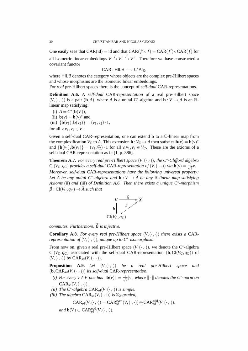
2(v+ iJv),where J is the complex structure of V .Moreover, CAR-representations have the following universal property: Let Abe any unital C∗-algebra anda : V → A be any anti-linear map satisfying Ax-ioms (ii) and (iii) of Definition A.1. Then there exists a unique C∗-morphism

28 CHRISTIAN BAR AND NICOLAS GINOUX
α : Cl(VC,qC)→ A such that
Va //
a
A
Cl(VC,qC)
α;;
commutes. Furthermore,α is injective.
Proof. Definep∓ :V →Cl(VC,qC) by p−(v) := 12(v+ iJv) andp+(v) := 1
2(v− iJv).Sincep−(Jv) =−ip−(v), the mapa= p− is anti-linear. Because ofa(v)−a(v)∗ =p−(v) + p+(v) = v, the C∗-subalgebra of Cl(VC,qC) generated by the image ofa containsV. Hencea(V) generates Cl(VC,qC) as a C∗-algebra. Axiom (i) inDefinition A.1 is proved.Let v1,v2 ∈V, then
a(v1),a(v2) = p−(v1) · p−(v2)+ p−(v2) · p−(v1)
= −2qC(p−(v1), p−(v2)) ·1= 0,
which is Axiom (ii) in Definition A.1. Furthermore,
a(v1)∗,a(v2) = −p+(v1) · p−(v2)− p−(v2) · p+(v1)
= 2qC(p+(v1), p−(v2)) ·1= Re(v1,v2) ·1+ iRe(v1,Jv2) ·1= (v1,v2) ·1,
which shows Axiom (iii) in Definition A.1. Therefore(a,Cl(VC,qC)) is a CAR-representation of(V,(· , ·)).The second part of the theorem follows from Cl(VC,qC) being simple, i.e.,from the non-existence of non-trivial closed two-sided∗-invariant ideals, see [31,Thm. 1.2.2]. Leta : V → A be any other anti-linear map satisfying (ii) and (iii)in Definition A.1. Sincea anda are injective (which is clear by Axiom (iii)) onemay setα(a(v)) := a(v) for all v∈V. Axioms (ii) and (iii) allow us to extendαto a C∗-morphismα : C∗(a(V)) = Cl(VC,qC)→ A. The injectivity ofa implies thenon-triviality of α which, together with the simplicity of Cl(VC,qC), provides theinjectivity of α . Therefore we found an injective C∗-morphismα : Cl(VC,qC)→ Awith α a= a. It is unique since it is determined bya anda on a subset of genera-tors. This concludes the proof of Theorem A.3.
For an alternative description of the CAR-representation in terms of creation andannihilation operators on the fermionic Fock space we referto [9, Prop. 5.2.2].
Corollary A.4. For every complex pre-Hilbert space(V,(· , ·)) there exists aCAR-representation of(V,(· , ·)), unique up to C∗-isomorphism.
Proof. The existence has already been proved in Theorem A.3. Let(a, A) be anyCAR-representation of(V,(· , ·)). Theorem A.3 states the existence of a uniqueinjective C∗-morphismα : Cl(VC,qC) → A such thatα a= a. Now α has to besurjective since Axiom (i) holds for(a, A).

CLASSICAL AND QUANTUM FIELDS ON LORENTZIAN MANIFOLDS 29
From now on, given a complex pre-Hilbert space(V,(· , ·)), we denote the C∗-algebra Cl(VC,qC) associated with the CAR-representation(a,Cl(VC,qC)) of(V,(· , ·)) by CAR(V,(· , ·)). We list the properties of CAR-representations whichare relevant for quantization, see also [9, Vol. II, Thm. 5.2.5, p. 15].
Proposition A.5. Let (V,(· , ·)) be a complex pre-Hilbert space and(a,CAR(V,(· , ·))) its CAR-representation.
(i) For every v∈ V one has‖a(v)‖ = |v| = (v,v)12 , where‖ · ‖ denotes the C∗-
norm onCAR(V,(· , ·)).(ii) The C∗-algebra CAR(V,(· , ·)) is simple, i.e., it has no closed two-sided∗-
ideals other than0 and the algebra itself.(iii) The algebraCAR(V,(· , ·)) isZ2-graded,
CAR(V,(· , ·)) = CAReven(V,(· , ·))⊕CARodd(V,(· , ·)),anda(V)⊂ CARodd(V,(· , ·)).
(iv) Let f :V →V ′ be an isometric linear embedding, where(V ′,(· , ·)′) is anothercomplex pre-Hilbert space. Then there exists a unique injective C∗-morphismCAR( f ) : CAR(V,(· , ·)) → CAR(V ′,(· , ·)′) such that
Vf
//
a
V ′
a′
CAR(V,(· , ·)) CAR( f )// CAR(V ′,(· , ·)′)
commutes.
Proof. We show assertion (i) . On the one hand, the C∗-property of the norm‖ · ‖implies
‖a(v)‖4 = ‖a(v)a(v)∗‖2
= ‖(a(v)a(v)∗)2‖.On the other hand,
(a(v)a(v)∗)2 = a(v)a(v)∗ ,a(v)a(v)∗
= |v|2a(v)a(v)∗,
where we useda(v)2 = 0 which follows from the second axiom. We deduce that
‖a(v)‖4 = |v|2 · ‖a(v)a(v)∗‖= |v|2 · ‖a(v)‖2.
Sincea is injective, we obtain the result.Assertion (ii) follows from Cl(VC,qC) being simple, see [31, Thm. 1.2.2]. Alterna-tively, it can be deduced from the universal property formulated in Theorem A.3.To see (iii) we recall that the Clifford algebra Cl(VC,qC) has aZ2-grading wherethe even part is generated by products of an even number of vectors inVC and,similarly, the odd part is the vector space span of products of an odd number ofvectors inVC, see [31, p. 27]. This is compatible with the Clifford relations (15).Clearly,a(V)⊂ CARodd(V,(· , ·)).It remains to show (iv). It is straightforward to check thata′ f satisfies Axioms (ii)and (iii) in Definition A.1. The result follows from Theorem A.3.
30 CHRISTIAN BAR AND NICOLAS GINOUX
One easily sees that CAR(id) = id and that CAR( f ′ f ) = CAR( f ′)CAR( f ) for
all isometric linear embeddingsVf−→ V ′ f ′−→ V ′′. Therefore we have constructed a
covariant functorCAR :HILB−→ C∗Alg,
whereHILB denotes the category whose objects are the complex pre-Hilbert spacesand whose morphisms are the isometric linear embeddings.For real pre-Hilbert spaces there is the concept ofself-dualCAR-representations.
Definition A.6. A self-dual CAR-representationof a real pre-Hilbert space(V,(· , ·)) is a pair(b,A), whereA is a unital C∗-algebra andb : V → A is anR-linear map satisfying:
(i) A=C∗(b(V)),(ii) b(v) = b(v)∗ and(iii) b(v1),b(v2)= (v1,v2) ·1,
for all v,v1,v2 ∈V.
Given a self-dual CAR-representation, one can extendb to aC-linear map fromthe complexificationVC to A. This extensionb : VC → A then satisfiesb(v) = b(v)∗
andb(v1),b(v2) = (v1, v2) · 1 for all v,v1,v2 ∈ VC. These are the axioms of aself-dual CAR-representation as in [1, p. 386].
Theorem A.7. For every real pre-Hilbert space(V,(· , ·)), the C∗-Clifford algebraCl(VC,qC) provides a self-dualCAR-representation of(V,(· , ·)) via b(v) = i√
2v.
Moreover, self-dualCAR-representations have the following universal property:Let A be any unital C∗-algebra andb : V → A be anyR-linear map satisfyingAxioms(ii) and (iii) of Definition A.6. Then there exists a unique C∗-morphismβ : Cl(VC,qC)→ A such that
Vb //
b
A
Cl(VC,qC)
β;;
commutes. Furthermore,β is injective.
Corollary A.8. For every real pre-Hilbert space(V,(· , ·)) there exists aCAR-representation of(V,(· , ·)), unique up to C∗-isomorphism.
From now on, given a real pre-Hilbert space(V,(· , ·)), we denote the C∗-algebraCl(VC,qC) associated with the self-dual CAR-representation(b,Cl(VC,qC)) of(V,(· , ·)) by CARsd(V,(· , ·)).Proposition A.9. Let (V,(· , ·)) be a real pre-Hilbert space and(b,CARsd(V,(· , ·))) its self-dualCAR-representation.
(i) For every v∈V one has‖b(v)‖ = 1√2|v|, where‖ · ‖ denotes the C∗-norm on
CARsd(V,(· , ·)).(ii) The C∗-algebraCARsd(V,(· , ·)) is simple.(iii) The algebraCARsd(V,(· , ·)) isZ2-graded,
CARsd(V,(· , ·)) = CARevensd (V,(· , ·))⊕CARodd
sd (V,(· , ·)),andb(V)⊂ CARodd
sd (V,(· , ·)).

CLASSICAL AND QUANTUM FIELDS ON LORENTZIAN MANIFOLDS 31
(iv) Let f :V →V ′ be an isometric linear embedding, where(V ′,(· , ·)′) is anotherreal pre-Hilbert space. Then there exists a unique injective C∗-morphismCARsd( f ) : CARsd(V,(· , ·)) → CARsd(V ′,(· , ·)′) such that
Vf
//
b
V ′
b′
CARsd(V,(· , ·))CARsd( f )
// CARsd(V ′,(· , ·)′)commutes.
The proofs are similar to the ones for CAR-representations of complex pre-Hilbertspaces. We have constructed a functor
CARsd : HILBR −→ C∗Alg,
whereHILBR denotes the category whose objects are the real pre-Hilbertspacesand whose morphisms are the isometric linear embeddings.
Remark A.10. Let (V,(· , ·)) be a complex pre-Hilbert space. If we considerV asa real vector space, then we have the real pre-Hilbert space(V,Re(· , ·)). For thecorresponding CAR-representations we have
CAR(V,(· , ·)) = CARsd(V,Re(· , ·)) = Cl(VC,qC)
and
b(v) =i√2(a(v)−a(v)∗).
A.2. CCR algebras. In this section, we recall the construction of the representa-tion of any (real) symplectic vector space by the so-called canonical commutationrelations (CCR). Proofs can be found in [4, Sec. 4.2].
Definition A.11. A CCR-representationof a symplectic vector space(V,ω) is apair (w,A), whereA is a unital C∗-algebra andw is a mapV → A satisfying:
(i) A=C∗(w(V)),(ii) w(0) = 1,(iii) w(−ϕ) = w(ϕ)∗,(iv) w(ϕ +ψ) = eiω(ϕ ,ψ)/2w(ϕ) ·w(ψ),
for all ϕ ,ψ ∈V.
The mapw is in general neither linear, nor any kind of group homomorphism, norcontinuous [4, Prop. 4.2.3].
Example A.12. Given any symplectic vector space(V,ω), consider the HilbertspaceH := L2(V,C), whereV is endowed with the counting measure. Define themapw from V into the spaceL (H) of bounded endomorphisms ofH by
(w(ϕ)F)(ψ) := eiω(ϕ ,ψ)/2F(ϕ +ψ),
for all ϕ ,ψ ∈V andF ∈ H. It is well-known thatL (H) is a C∗-algebra with theoperator norm as C∗-norm, and that the mapw satisfies the Axioms (ii)-(iv) fromDefinition A.11, see e.g. [4, Ex. 4.2.2]. Hence settingA := C∗(w(V)), the pair(w,A) provides a CCR-representation of(V,ω).
This is essentially the only example of CCR-representation:

32 CHRISTIAN BAR AND NICOLAS GINOUX
Theorem A.13. Let (V,ω) be a symplectic vector space and(w, A) be a pairsatisfying the Axioms(ii) -(iv) of Definition A.11. Then there exists a unique C∗-morphismΦ : A→ A such thatΦw= w, where(w,A) is theCCR-representationfrom Example A.12. Moreover,Φ is injective.In particular, (V,ω) has aCCR-representation, unique up to C∗-isomorphism.
We denote the C∗-algebra associated to the CCR-representation of(V,ω) fromExample A.12 by CCR(V,ω). As a consequence of Theorem A.13, we obtain thefollowing important corollary.
Corollary A.14. Let (V,ω) be a symplectic vector space and(w,CCR(V,ω)) itsCCR-representation.
(i) The C∗-algebraCCR(V,ω) is simple, i.e., it has no closed two-sided∗-idealsother than0 and the algebra itself.
(ii) Let (V ′,ω ′) be another symplectic vector space and f: V → V ′ a symplec-tic linear map. Then there exists a unique injective C∗-morphismCCR( f ) :CCR(V,ω)→ CCR(V ′,ω ′) such that
Vf
//
w
V ′
w′
CCR(V,ω)CCR( f )
// CCR(V ′,ω ′)
commutes.
Obviously CCR(id) = id and CCR( f ′ f ) = CCR( f ′)CCR( f ) for all symplectic
linear mapsVf→V ′ f ′→V ′′, so that we have constructed a covariant functor
CCR :Sympl−→ C∗Alg.
REFERENCES
[1] H. A RAKI : On quasifree states ofCAR and Bogoliubov automorphisms. Publ. Res. Inst. Math.Sci.6 (1970/71), 385–442.
[2] C. BAR AND C. BECKER: C∗-algebras. In: C. Bar and K. Fredenhagen (Eds.):Quantum fieldtheory on curved spacetimes. 1-37, Lecture Notes in Phys.786, Springer-Verlag, Berlin, 2009.
[3] C. BAR, P. GAUDUCHON, AND A. M OROIANU: Generalized Cylinders in Semi-Riemannianand Spin Geometry. Math. Zeitschr.249(2005), 545–580.
[4] C. BAR, N. GINOUX , AND F. PFAFFLE: Wave Equations on Lorentzian Manifolds and Quan-tization. EMS, Zurich, 2007.
[5] H. BAUM : Spin-Strukturen und Dirac-Operatoren uber pseudoriemannschen Mannig-faltigkeiten. Teubner, Leipzig, 1981.
[6] A. N. BERNAL AND M. SANCHEZ: Smoothness of time functions and the metric splitting ofglobally hyperbolic spacetimes. Commun. Math. Phys.257(2005), 43–50.
[7] A. N. BERNAL AND M. SANCHEZ: Further results on the smoothability of Cauchy hypersur-faces and Cauchy time functions. Lett. Math. Phys.77 (2006), 183–197.
[8] T. BRANSON AND O. HIJAZI : Bochner-Weitzenbock formulas associated with the Rarita-Schwinger operator. Internat. J. Math.13 (2002), 137–182.
[9] O. BRATTELI AND D. W. ROBINSON: Operator algebras and quantum statistical mechanics,I-II (second edition). Texts and Monographs in Physics, Springer, Berlin, 1997.
[10] T. BROCKER AND T. TOM DIECK: Representations of compact Lie groups. Graduate Texts inMathematics98, Springer-Verlag, New York, 1995.
[11] R. BRUNETTI, K. FREDENHAGEN ANDR. VERCH: The generally covariant locality principle- a new paradigm for local quantum field theory. Commun. Math. Phys.237(2003), 31–68.

CLASSICAL AND QUANTUM FIELDS ON LORENTZIAN MANIFOLDS 33
[12] H. A. BUCHDAHL : On the compatibility of relativistic wave equations in Riemann spaces. II.J. Phys. A15 (1982), 1-5.
[13] H. A. BUCHDAHL : On the compatibility of relativistic wave equations in Riemann spaces. III.J. Phys. A15 (1982), 1057-1062.
[14] C. DAPPIAGGI, T.-P. HACK AND N. PINAMONTI : The extended algebra of observables forDirac fields and the trace anomaly of their stress-energy tensors. Rev. Math. Phys.21 (2009),1241–1312.
[15] C. DAPPIAGGI, V. MORETTI AND N. PINAMONTI : Distinguished quantum states in a classof cosmological spacetimes and their Hadamard property. J. Math. Phys.50 (2009), 062304,38 p.
[16] C. DAPPIAGGI, N. PINAMONTI AND M. PORRMANN: Local causal structures, Hadamardstates and the principle of local covariance in quantum fieldtheory. arXiv:1001.0858
[17] J. DIMOCK : Algebras of local observables on a manifold. Commun. Math. Phys.77 (1980),219–228.
[18] J. DIMOCK : Dirac quantum fields on a manifold. Trans. Amer. Math. Soc.269 (1982), 133–147.
[19] C. J. FEWSTER ANDR. VERCH: A quantum weak energy inequality for Dirac fields in curvedspacetime. Commun. Math. Phys.225(2002), 331–359.
[20] E. FURLANI : Quantization of massive vector fields in curved space-time. J. Math. Phys.40(1999), 2611-2626.
[21] R.P. GEROCH: Domain of dependence. J. Math. Phys.11 (1970), 437–449.[22] G. W. GIBBONS: A note on the Rarita-Schwinger equation in a gravitational background.
J. Phys. A9 (1976), 145–148.[23] L. HORMANDER: The analysis of linear partial differential operators. I. Distribution theory
and Fourier analysis. 2nd ed. Grundlehren der Mathematischen Wissenschaften256, Springer-Verlag, Berlin, 1990.
[24] L. HORMANDER: The analysis of linear partial differential operators. III. Pseudodifferen-tial operators. Grundlehren der Mathematischen Wissenschaften274, Springer-Verlag, Berlin,1985.
[25] S. HOLLANDS AND R. M. WALD : Axiomatic quantum field theory in curved spacetime. Com-mun. Math. Phys.293(2010), 85–125.
[26] B. S. KAY: Linear spin-zero quantum fields in external gravitational and scalar fields. Com-mun. Math. Phys.62 (1978), 55–70.
[27] H. B. LAWSON AND M.-L. M ICHELSOHN: Spin Geometry. Princeton University Press,Princeton, 1989.
[28] R. MUHLHOFF: Higher Spin fields on curved spacetimes. Diplomarbeit, Universitat Leipzig,2007.
[29] R. MUHLHOFF: Cauchy Problem and Green’s Functions for First Order Differential Operatorsand Algebraic Quantization. J. Math. Phys.52 (2011), 022303, 7 p.
[30] B. O’NEILL : Semi-Riemannian Geometry. Academic Press, San Diego, 1983.[31] R. J. PLYMEN AND P.L. ROBINSON: Spinors in Hilbert space. Cambridge Tracts in Mathe-
matics114, Cambridge University Press, Cambridge, 1994.[32] M. J. RADZIKOWSKI : Micro-local approach to the Hadamard condition in quantum field the-
ory on curved space-time. Commun. Math. Phys.179(1996), 529-553.[33] W. RARITA AND J. SCHWINGER: On a Theory of Particles with Half-Integral Spin. Phys.
Rev.60 (1941), 61.[34] M. REED AND B. SIMON : Methods of Modern Mathematical Physics I: Functional Analysis.
Academic Press, Orlando, 1980.[35] M. REED AND B. SIMON : Methods of Modern Mathematical Physics II: Fourier Analysis,
Self-Adjointness. Academic Press, Orlando, 1975.[36] H. SAHLMANN AND R. VERCH: Passivity and microlocal spectrum condition. Commun.
Math. Phys.214(2000), 705–731.[37] H. SAHLMANN AND R. VERCH: Microlocal spectrum condition and Hadamard form for
vector-valued quantum fields in curved spacetime. Rev. Math. Phys.13 (2001), 1203–1246.[38] K. SANDERS: The locally covariant Dirac field. Rev. Math. Phys. 22 (2010), 381–430.[39] A. STROHMAIER: The Reeh-Schlieder property for quantum fields on stationary spacetimes.
Commun. Math. Phys.215(2000), 105–118.
34 CHRISTIAN BAR AND NICOLAS GINOUX
[40] M. E. TAYLOR : Partial Differential Equations I - Basic Theory. Springer-Verlag, New York -Berlin - Heidelberg, 1996.
[41] R. VERCH: A spin-statistics theorem for quantum fields on curved spacetime manifolds in agenerally covariant framework. Commun. Math. Phys.223(2001), 261–288.
[42] R. M. WALD : Quantum field theory in curved spacetime and black hole thermodynamics.University of Chicago Press, Chicago, 1994.
[43] MCK. Y. WANG: Preserving parallel spinors under metric deformations. Indiana Univ. Math.J.40 (1991), 815–844.
[44] V. WUNSCH: Cauchy’s problem and Huygens’ principle for relativistic higher spin wave equa-tions in an arbitrary curved space-time. Gen. Relativity Gravitation17 (1985), 15-38.
UNIVERSITAT POTSDAM, INSTITUT FUR MATHEMATIK , AM NEUEN PALAIS 10, HAUS 8, 14469POTSDAM, GERMANY
FAKULT AT FUR MATHEMATIK , UNIVERSITAT REGENSBURG, 93040 REGENSBURG, GERMANY
E-mail address: [email protected] address: [email protected]