Class 26

Model Building Philosophy

Pfeifer note: Section 6

Assignment 26• 1. T-test 2-sample ≡ regression with dummy

T= +/- 6.2/2.4483 (from data analysis, complicated formula, OR regression with dummy)

• 2. ANOVA single factor ≡ regression with p-1 dummies (see next slide)

• 3. Better predictor? The one with lower regression standard error (or higher adj R2)– Not the one with the higher coefficient.

• 4. Will they charge less than $4,500?– Use regression’s standard error and t.dist to calculate

the probability.

LawyerPhysical Therapist Cabinetmaker

Systems Analyst

44 55 54 4442 78 65 7374 80 79 7142 86 69 6053 60 79 6450 59 64 6645 62 59 4148 52 78 5564 55 84 7638 50 60 62

Occupation SATLawyer 44Lawyer 42Lawyer 74Lawyer 42Lawyer 53Lawyer 50Lawyer 45Lawyer 48Lawyer 64Lawyer 38

Physical Therapist 55

Physical Therapist 78

Physical Therapist 80

Physical Therapist 86

Physical Therapist 60

Physical Therapist 59

Physical Therapist 62

Physical Therapist 52

Physical Therapist 55

Physical Therapist 50Cabinetmaker 54Cabinetmaker 65Cabinetmaker 79Cabinetmaker 69Cabinetmaker 79Cabinetmaker 64Cabinetmaker 59Cabinetmaker 78Cabinetmaker 84Cabinetmaker 60Systems Analyst 44Systems Analyst 73Systems Analyst 71Systems Analyst 60Systems Analyst 64Systems Analyst 66Systems Analyst 41Systems Analyst 55Systems Analyst 76Systems Analyst 62

SAT Dlawyer DPT Dcabinet44 1 0 042 1 0 074 1 0 042 1 0 053 1 0 050 1 0 045 1 0 048 1 0 064 1 0 038 1 0 055 0 1 078 0 1 080 0 1 086 0 1 060 0 1 059 0 1 062 0 1 052 0 1 055 0 1 050 0 1 054 0 0 165 0 0 179 0 0 169 0 0 179 0 0 164 0 0 159 0 0 178 0 0 184 0 0 160 0 0 144 0 0 073 0 0 071 0 0 060 0 0 064 0 0 066 0 0 041 0 0 055 0 0 076 0 0 062 0 0 0

Ready for ANOVA

Ready for Regression

Agenda

• IQ demonstration• What you can do with lots of data• What you should do with not much data• Practice using the Oakland As case

Remember the Coal Pile!

• Model Building involves more than just selecting which of the available X’s to include in the model.– See section 9 of the Pfeifer note to learn about

transforming X’s.– We won’t do much in this regard…

With lots of data (big data?)

X1 X2 . . Xn Y1 0.96 0.24 0.34 0.57 0.20 0.432 0.58 0.16 0.93 0.96 0.75 0.353 0.39 0.75 0.07 0.63 0.87 0.49. . . . . . .. . . . . . .N 0.47 0.34 0.69 0.86 0.30 0.22

X1 X2 . . Xn Y1 0.96 0.24 0.34 0.57 0.20 0.432 0.58 0.16 0.93 0.96 0.75 0.353 0.39 0.75 0.07 0.63 0.87 0.49. . . . . . .. . . . . . .

N1 0.21 0.76 0.44 0.07 0.65 0.92

X1 X2 . . Xn YN1+1 0.47 0.86 0.53 0.02 0.70 0.73N1+2 0.03 0.51 0.35 0.09 0.95 0.11N1+3 0.16 0.31 0.37 0.38 0.31 0.96

. . . . . . .

. . . . . . .N 0.47 0.34 0.69 0.86 0.30 0.22

1. Split the data into two sets

2. Use the training set to build several models.

3. Use the hold-out sample to test/compare the models. Use the best performing model.

Stats like “std error” and adj R-

square only measure FIT

Performance on a hold-out sample measures how well each model will FORECAST

With lots of data (big data?)

• Computer Algorithms do a very good job of finding a model

• They guard against “over-fitting”• Once you own the software, they are fast

and cheap• They won’t claim, however, to do better

than a professional model builder• Remember the coal pile!

Without much Data

• You will not be able to use a training set/hold out sample

• You get “one shot” to find a GOOD model• Regression and all its statistics can tell you which

model “FIT” the data the best.• Regression and all its statistics CANNOT tell you

which model will perform (forecast) the best.• Not to mention….regression has no clue about

what causes what…..

Remember…..

• The model that does a spectacular job of fitting the past….will do worse at predicting the future than a simpler model that more accurately captures the way the world works.

• Better fit leads to poorer forecasts!– Instead of forecasting 100 for the next IQ, the

over-fit model will sometimes predict 110 and other times predict 90!

Requiring low-p-values for all coefficients does not protect

against over-fitting.

• If there are 100 X’s that are of NO help in predicting Y,– We expect 5 of them will be statistically significant.– And we’ll want to use all 5 to predict the future.– And the model will be over-fit

– We won’t know it, perhaps– Our predictions will be WORSE as a result.

Modeling Balancing Act• Useable (do we know the

X’s?)• Simple • Make Sense

– Use your judgment, given you can’t solely rely on the stats/data

– Signs of coefficients should make sense

• Significant (low p) coefficients– Except for sets of dummies

• Low standard error– Consistent with high

adjusted R-square• Meets all four

assumptions– Linearity (most important)– Homoskedasticity (equal

variance)– Independence– Normality (least important)

Oakland As (A)

Case Facts

• Despite making only $40K, pitcher Mark Nobel had a great year for Oakland in 1980.– Second in the league for era (2.53), complete

games (24), innings (284-1/3), and strikeouts (180)– Gold glove winner (best fielding pitcher)– Second in CY YOUNG award voting.

Nobel Wants a Raise• “I’m not saying anything against Rick Langford or

Matt Keough (fellow As pitchers)…but I filled the stadium last year against Tommy John (star pitcher for the Yankees)”

• Nobel’s Agent argued– Avg. home attendance for Nobel’s 16 starts was

12,663.6– Avg. home attendance for remaining home games

was only 10,859.4– Nobel should get “paid” for the difference

• 1,804.2 extra tickets per start.

Data from 1980 Home GamesNo DATE TIX OPP POS GB DOW TEMP PREC TOG TV PROMO YANKS NOBEL1 10-Apr 24415 2 5 1 4 57 0 2 1 0 0 02 11-Apr 5729 2 3 1 5 66 0 2 1 0 0 03 12-Apr 5783 2 7 1 6 64 0 1 0 0 0 0. . . . . . . . . . . . . .. . . . . . . . . . . . . .

73 26-Sep 5099 6 2 14 5 64 0 2 1 0 0 174 27-Sep 4581 6 2 13 6 62 0 1 0 0 0 075 28-Sep 10662 6 2 12 7 65 0 1 0 1 0 0

                       LEGEND       Opposing Team Position: A's ranking in American League West   

  1Seattle 8White SoxGames Behind: Minimum No of games needed to move ahead of current first place team.

  2Minnesota 9Boston  

  3California 10Baltimore Day of Week: Monday=1, Tuesday=2, etc.

  4Yankees 11Cleveland  5Detroit 12Texas Precipitation: 1 if precipitation, 0 if not.

  6Milwaukee 13Kansas City

  7Toronto Time of Game: 1 if day, 2 if night                     

TASK• Be ready to report about the model assigned to your table (1 to 7)

– What is the model? (succinct)– Critique it (succinctly)

– Ignore “durban watson”– “standard deviation of residuals” aka regression’s standard error.– Output gives just t-stat. A t of +- 2 corresponds to p-value of 0.05.

Model 1: TIX versus NOBEL Variable Coefficient Std. Error T-stat. NOBEL 1,804.207 2,753.164 0.655 CONSTANT 10,859.356 1,271.632 8.540 R-Squared = 0.006 Std. Deviation of Residuals = 9767.6 Adjusted R-Square = -0.008 Durbin Watson D = 1.196

Model 4: TIX versus OPP, NOBEL

Variable Coefficient Std. Error T-stat. OPP -269.135 297.809 -0.904 NOBEL 1,572.135 2,768.562 0.568 CONSTANT 12,807.161 2,182.002 5.869 R-Squared = 0.017 Std. Deviation of Residuals = 9779.9 Adjusted R-Square = 0.010 Durbin Watson D = 1.146

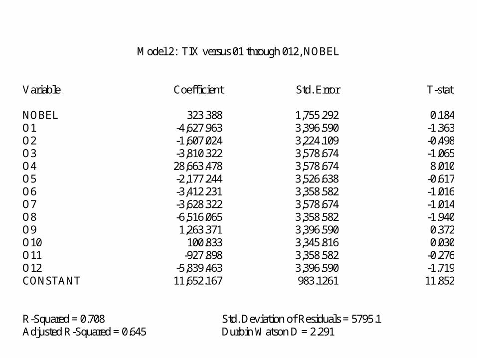
Model 2: TIX versus 01 through 012, NOBEL Variable Coefficient Std. Error T-stat. NOBEL 323.388 1,755.292 0.184 O1 -4,627.963 3,396.590 -1.363 O2 -1,607.024 3,224.109 -0.498 O3 -3,810.322 3,578.674 -1.065 O4 28,663.478 3,578.674 8.010 O5 -2,177.244 3,526.638 -0.617 O6 -3,412.231 3,358.582 -1.016 O7 -3,628.322 3,578.674 -1.014 O8 -6,516.065 3,358.582 -1.940 O9 1,263.371 3,396.590 0.372 O10 100.833 3,345.816 0.030 O11 -927.898 3,358.582 -0.276 O12 -5,839.463 3,396.590 -1.719 CONSTANT 11,652.167 983.1261 11.852 R-Squared = 0.708 Std. Deviation of Residuals = 5795.1 Adjusted R-Squared = 0.645 Durbin Watson D = 2.291

Model 3: TIX versus O1 through O12, PREC, TEMP, PROMO, NOBEL, OD, DH

Variable Coefficient Std. Error T-stat. PREC -3,772.043 3,383.418 -1.115 TEMP -184.293 237.731 -0.775 PROMO 5,398.545 1,780.857 3.031 NOBEL -403.502 1,518.000 -0.266 OD 15,382.632 5,652.397 2.721 DH 7,645.224 2,429.894 3.146 O1 -7,213.660 2,999.437 -2.405 O2 -3,203.395 3,046.540 -1.051 O3 -5,780.245 3,242.464 -1.783 O4 25,640.501 3,196.000 8.023 O5 -3,444.192 3,056.500 -1.127 O6 -4,568.433 2,988.677 -1.529 O7 -5,075.192 3,190.707 -1.591 O8 -5,973.904 3,329.604 -1.794 O9 1,966.401 2,971.357 0.662 O10 -2,352.715 3,002.119 -0.784 O11 -1,701.151 3,023.445 -0.563 O12 -5,627.881 2,911.665 -1.933 CONSTANT 22,740.489 14,777.323 1.539 R-Squared = 0.803 Std. Deviation of Residuals = 5011.0 Adjusted R-Squared = 0.740 Durbin Watson D = 2.269

Model 5: TIX versus PREC, TOG, TV, PROMO, NOBEL, YANKS, WKEND, OD, DH Variable Coefficient Std. Error T-stat. PREC -3,660.109 3,251.502 -1.126 TOG 1,606.406 1,334.121 1.204 TV 223.421 1,982.301 0.113 PROMO 4,382.173 1,658.644 2.642 NOBEL -1,244.411 1,546.545 -0.805 YANKS 29,493.164 2,532.314 11.647 WKEND 1,468.269 1,328.585 1.105 OD 16,119.831 5,388.174 2.992 DH 5,815.814 2,375.194 2.449 CONSTANT 5,082.356 2,170.419 2.342 R-Squared = 0.742 Std. Deviation of Residuals = 5273.5 Adjusted R-Squared = 0.706 Durbin Watson D = 1.733

Model 6: TIX versus PROMO, NOBEL, YANKS, DH

Variable Coefficient Std. Error T-stat. PROMO 4,195.743 1,737.742 2.414 NOBEL -1,204.082 1,607.869 -0.749 YANKS 29,830.245 2,641.516 11.293 DH 5,274.262 2,457.377 2.146 CONSTANT 8,363.238 527.298 15.861 R-Squared = 0.692 Std. Deviation of Residuals = 5551.0 Adjusted R-Square = 0.675 Durbin Watson D = 1.96

Model 7: TIX versus PREC, PROMO, NOBEL, YANKS, OD Variable Coefficient Std. Error T-stat. PREC -1,756.508 3,227.439 -0.544 PROMO 3,758.92 1,687.895 2.227 NOBEL -209.484 1,549.192 -0.135 YANKS 30,568.223 2,570.535 11.892 OD 15,957.998 5,491.220 2.906 CONSTANT 8,457.002 496.203 17.043 R-Squared = 0.709 Std. Deviation of Residuals = 5434.5 Adjusted R-Square = 0.688 Durbin Watson D = 1.873

What does it mean that the coefficient of NOBEL in negative in most of the

models?

Why was the coefficient of NOBEL positive in model 1?