civil engineering 394k: topic 3 geographic information ... · juhn-yuan su (js56859) c e 394k term...

Civil Engineering 394K:

Topic 3

Geographic Information Systems (GIS) in Water

Resources Engineering

TERM PROJECT REPORT

Reinvestigation of the Halloween Flood and Hydrologic

Modeling of the Onion Creek Watershed

FALL 2014

Written By: Juhn-Yuan Su (js56859), M.S. Student in EWRE

Instructor: Dr. D. R. Maidment (University of Texas at Austin)

Course: C E 394K: Geographic Information Systems in Water Resources

Class Time: Tuesdays and Thursdays 12:30 to 2 PM, ETC 5.148

Unique Number: 16185

Juhn-Yuan Su (js56859) C E 394K Term Project Report Dr. D. R. Maidment

i

TABLE OF CONTENTS Term Project: Revisit of Halloween Creek Flooding ..................................................................... 1

Background ..................................................................................................................................... 1

Project Analysis .............................................................................................................................. 1

Analysis of Previous Studies ....................................................................................................... 2

Project Approach ......................................................................................................................... 2

ArcHydro Preprocessing .......................................................................................................... 2

Soil and Land Use.................................................................................................................... 6

HEC-GeoHMS Processing: Basin and River ........................................................................ 10

HEC-GeoHMS Processing: Flows and Grid Cells ................................................................ 10

Exporting the Files onto HMS ............................................................................................... 12

Generating HMS Project and Simulating Runs ..................................................................... 14

Conclusion .................................................................................................................................... 17

References ..................................................................................................................................... 18

Appendix A: HMS Maps ............................................................................................................ A-1

Map of Reaches ....................................................................................................................... A-1

Subbasin Map .......................................................................................................................... A-2

List of Tables Table 1: Curve Number Lookup Table for Land Use and Soil Type ............................................. 8

Table 2: Simulation Results from HMS Run ................................................................................ 15

List of Figures Figure 1: Onion Creek Watershed with HUC 12 Basins relative to Austin ................................... 1

Figure 2: Filled DEM over the Onion Creek Watershed ................................................................ 3

Figure 3: Flow Direction Raster Dataset ........................................................................................ 3

Figure 4: Flow Accumulation Grid ................................................................................................. 4

Figure 5: Stream Definition Generated from Flow Accumulation through Raster Calculator ....... 4

Figure 6: Stream Definition Grid .................................................................................................... 4

Figure 7: Stream Link and Catchment Grid .................................................................................... 5

Figure 8: Drainage Lines and Catchment Polygons over Onion Creek .......................................... 5

Figure 9: Soil Hydrologic Groups in the Onion Creek Watershed ................................................. 6

Figure 10: Coding of PctB over the Onion Creek Watershed ........................................................ 7

Figure 11: Curve Number Grid over Onion Creek Watershed ....................................................... 9

Figure 12: Percent Impervious Grid over Onion Creek Watershed ................................................ 9

Figure 13: Grid Cell Intersect Class from Grid Cell Processing .................................................. 11

Figure 14: Required Files for Map to HMS Units ........................................................................ 12


ii

Figure 15: HMS Schematic for Onion Creek Watershed ............................................................. 12

Figure 16: Precipitation over October 31, 2013............................................................................ 13

Figure 17: Thiessen Polygon Generated ....................................................................................... 13

Figure 18: Depth and Time Weights for a Selected Subbasin in HMS ........................................ 14

Figure 19: HMS Model for the Onion Creek Watershed .............................................................. 14

Figure 20: Precipitation Gage Properties for Time-Series Data ................................................... 15

Figure 21: Precipitation Time-Series Data Inputted Manually ..................................................... 15

Figure 22: Flow Profile for Reach R50 in HMS ........................................................................... 17


1

Term Project: Revisit of Halloween Creek Flooding

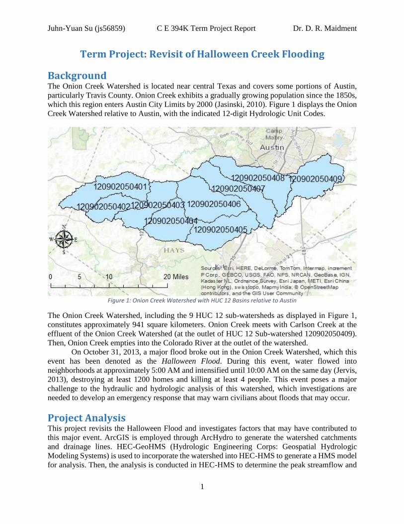
Background The Onion Creek Watershed is located near central Texas and covers some portions of Austin,

particularly Travis County. Onion Creek exhibits a gradually growing population since the 1850s,

which this region enters Austin City Limits by 2000 (Jasinski, 2010). Figure 1 displays the Onion

Creek Watershed relative to Austin, with the indicated 12-digit Hydrologic Unit Codes.

Figure 1: Onion Creek Watershed with HUC 12 Basins relative to Austin

The Onion Creek Watershed, including the 9 HUC 12 sub-watersheds as displayed in Figure 1,

constitutes approximately 941 square kilometers. Onion Creek meets with Carlson Creek at the

effluent of the Onion Creek Watershed (at the outlet of HUC 12 Sub-watershed 120902050409).

Then, Onion Creek empties into the Colorado River at the outlet of the watershed.

On October 31, 2013, a major flood broke out in the Onion Creek Watershed, which this

event has been denoted as the Halloween Flood. During this event, water flowed into

neighborhoods at approximately 5:00 AM and intensified until 10:00 AM on the same day (Jervis,

2013), destroying at least 1200 homes and killing at least 4 people. This event poses a major

challenge to the hydraulic and hydrologic analysis of this watershed, which investigations are

needed to develop an emergency response that may warn civilians about floods that may occur.

Project Analysis This project revisits the Halloween Flood and investigates factors that may have contributed to

this major event. ArcGIS is employed through ArcHydro to generate the watershed catchments

and drainage lines. HEC-GeoHMS (Hydrologic Engineering Corps: Geospatial Hydrologic

Modeling Systems) is used to incorporate the watershed into HEC-HMS to generate a HMS model

for analysis. Then, the analysis is conducted in HEC-HMS to determine the peak streamflow and


2

the time for this to occur. Assumptions have been made to simplify this project to a small-scale

revisit of the Halloween Flood for calculating the peak streamflow.

Analysis of Previous Studies Much research has been conducted toward predicting streamflow from given precipitation data for

a watershed. Much of the general parameters are needed for calculating streamflow from

precipitation data, involving the storage over time, the evapotranspiration of the watershed, and

the infiltration into the land. However, while these variables (evapotranspiration, infiltration, and

storage) are fundamental for determining the streamflow for the watershed, such parameters are

affected by the surrounding environment. For instance, increasing temperature over northern

regions pose significant concern on whether the streamflow for the region increases, such as

Northern Russia (Adam & Lettenmaider, 2008). GIS is also employed for incorporating

groundwater recharge for a mountain river for calculating streamflow in Taiwan (Yeh, et al., 2014).

Landuse and geological information are integrated into the watershed and then processed by GIS

to develop a groundwater potential zone map (Yeh, et al., 2014), which can then be used to

determine the streamflow through the watershed. Meanwhile, Tobin and Bennett (2014)

incorporated two models, the Soil and Water Assessment Tool with the Gridded Surface and

Subsurface Hydrologic Analysis, toward predicting streamflow from the given precipitation data.

The complexity of the models are tested to understand the impacts upon streamflow calculations

for varying precipitation data (Tobin & Bennett, 2014).

Approaches for calculating streamflow from given precipitation data are researched based

on previous journal articles and studies. For instance, a conceptual model that divides streamflow

into baseflow, interflow (between surface and underground), and surface flow is used for analyzing

precipitation data for a watershed (Rimmer & Salingar, 2006). On the other hand, Patterson et al.

(2012) analyzed streamflow changes in the southeastern United States region over time. A

regression analysis was developed to relate streamflow changes with precipitation in response to

droughts during the late 1900s (Patterson, Lutz, & Doyle, 2012). Han (2010) performed a small-

scale analysis of streamflow prediction incorporating sets of precipitation time series data based

on distinct moisture conditions. Both GIS and HEC-GeoHMS were incorporated to compute

streamflow for the generated subbasins of the San Antonio River Watershed (Han, 2010). At the

same time, another study involves the incorporation of GIS into studying subbasin and reach lag

time for streamflow calculation (Costache, 2014). These investigations have been analyzed to

understand a general procedure for predicting streamflow from precipitation data for the Onion

Creek Watershed.

Project Approach The Onion Creek Watershed has been extracted from the ArcMap package provided by Dr. David

Tarboton at the University of North Carolina at Chapel Hill, as shown in Figure 1 above. The

following approaches are generally employed for this project:

ArcHydro Preprocessing The general Digital Elevation Model (N30m) provided by the United States Geological Survey

(USGS) is used for the ArcHydro Preprocessing portion, and the DEM is then extracted over the

watershed buffer. ArcHydro and HEC-GeoHMS are used to generate the watershed basins and the

drainage lines that are then imported into HEC-HMS for analysis. The following procedures are

employed for processing the Digital Elevation Model of the Onion Creek Watershed:


3

1) Filling the DEM: All the pits in the watershed are filled using the general fill

geoprocessing tool studied in class. Figure 2 corresponds to the Filled DEM for the Onion

Creek Watershed.

Figure 2: Filled DEM over the Onion Creek Watershed

2) Flow Direction: The Eight-Point Model has been used to determine the flow direction over

the watershed, as displayed in Figure 3.

Figure 3: Flow Direction Raster Dataset

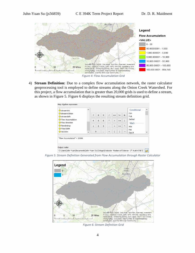
3) Flow Accumulation: The flow accumulation geoprocessing tool is employed to determine

the cumulative area flowing into a particular grid using the flow direction feature class

generated from step 2. Figure 4 displays the flow accumulation grid.


4

Figure 4: Flow Accumulation Grid

4) Stream Definition: Due to a complex flow accumulation network, the raster calculator

geoprocessing tool is employed to define streams along the Onion Creek Watershed. For

this project, a flow accumulation that is greater than 20,000 grids is used to define a stream,

as shown in Figure 5. Figure 6 displays the resulting stream definition grid.

Figure 5: Stream Definition Generated from Flow Accumulation through Raster Calculator

Figure 6: Stream Definition Grid


5

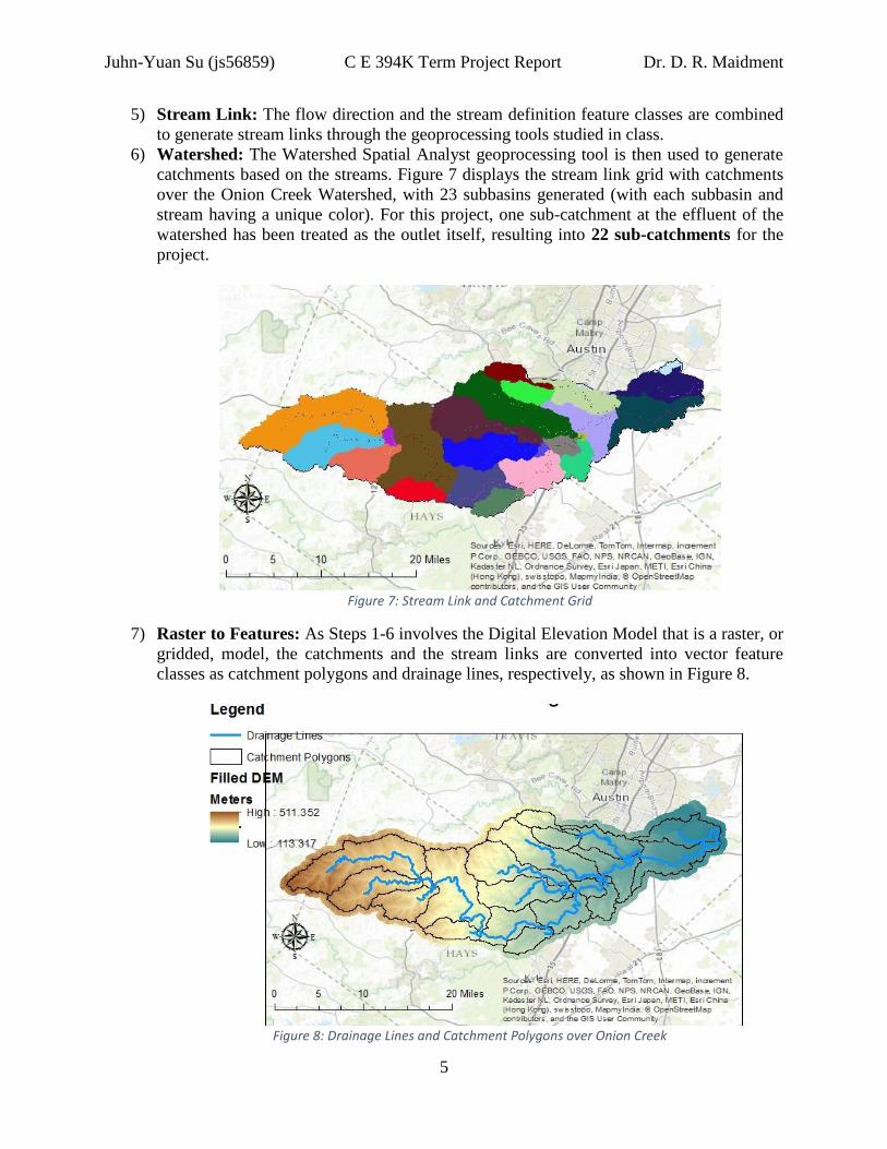
5) Stream Link: The flow direction and the stream definition feature classes are combined

to generate stream links through the geoprocessing tools studied in class.

6) Watershed: The Watershed Spatial Analyst geoprocessing tool is then used to generate

catchments based on the streams. Figure 7 displays the stream link grid with catchments

over the Onion Creek Watershed, with 23 subbasins generated (with each subbasin and

stream having a unique color). For this project, one sub-catchment at the effluent of the

watershed has been treated as the outlet itself, resulting into 22 sub-catchments for the

project.

Figure 7: Stream Link and Catchment Grid

7) Raster to Features: As Steps 1-6 involves the Digital Elevation Model that is a raster, or

gridded, model, the catchments and the stream links are converted into vector feature

classes as catchment polygons and drainage lines, respectively, as shown in Figure 8.

Figure 8: Drainage Lines and Catchment Polygons over Onion Creek


6

8) Adjoint Catchment Processing: The catchment polygons and the stream links that are

converted into vector feature classes are then aggregated, with the catchment polygons

dissolved into a single subbasin using the HEC-GeoHMS preprocessing tools.

The catchment polygons and the drainage lines are then used by HEC-GeoHMS to generate a new

HMS project for further analysis.

Soil and Land Use Soil data has been gathered through the Soil Survey Geographic (SSURGO) service for Travis

County, including information related to the hydrologic soil group that classifies soils based on

their properties, such as the general infiltration rate. Land Use data has been gathered through the

National Land Cover Database (NLCD), which the 2011 version has been used. The following

procedures are implemented for determining a curve number grid, which is essential for

calculating excess precipitation over the watershed:

1) Extract by Mask and Intersect: The land use data, a raster dataset, covers the entire

United States and are hence extracted for the Onion Creek Watershed. Soil data over Travis

County, a vector feature class, is intersected with the adjoint Onion Creek Watershed to

yield soil information over this watershed only rather than the entire county.

2) Combine Land Use and Soil Data: Both the land use and soil data that are extracted for

the Onion Creek Watershed are then intersected to determine the corresponding land use

and soil type for a given area.

3) Curve Number Lookup Table: Using the TR-55 Reference Manual (Cronshey, et al.,

1986) and a general guide that approximates curve numbers for forests and agricultural

purposes (Merwade, 2012), a curve number table has been developed based on the land use

and soil type.

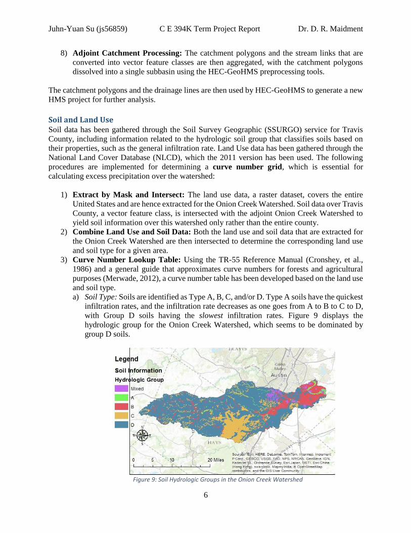
a) Soil Type: Soils are identified as Type A, B, C, and/or D. Type A soils have the quickest

infiltration rates, and the infiltration rate decreases as one goes from A to B to C to D,

with Group D soils having the slowest infiltration rates. Figure 9 displays the

hydrologic group for the Onion Creek Watershed, which seems to be dominated by

group D soils.

Figure 9: Soil Hydrologic Groups in the Onion Creek Watershed


7

As shown in Figure 9, there are regions where the soil type is rather unknown. For this

project, a grid with a given soil type is identified as 100% of that type (e.g., soil

identified as “A” will be “100% Type A”). On the other hand, the soil type that is

undefined is assumed to be an equal mix of all the groups (25% Type A, 25% Type B,

25% Type C, and 25% Type D). Therefore, four columns are generated in the Soil Type

Attribute Table with “PctA”, “PctB”, “PctC”, and “PctD” (which are required fields

for the curve number grid). Using field calculator, a short Python Code is implemented,

which is shown for “PctB” as follows (into the source block, with HG as the hydrologic

group):

def reclass(HG):

if HG = = “B”:

return 100

elif HG = = “ ”:

return 25

else:

return 0

Figure 10 displays the code input into the field calculator for the soil type attribute table

over the Onion Creek Watershed.

Figure 10: Coding of PctB over the Onion Creek Watershed


8

b) Soil Type and Land Use Curve Number Lookup Grid: TR-55 and Merwade (2012) are

referenced for determining the curve number for a given land use and soil hydrologic

group. Table 1 displays the curve number lookup table and the land use definitions

based on the values (“LUValue”) shown.

Table 1: Curve Number Lookup Table for Land Use and Soil Type

c) Land Use: For the Curve Number Grid, the parameter PctImp (Percent Impervious) is

required but not defined in the land use data. The PctImp is programmed similarly as

the PctA (and the other soil groups) for a given land use (written as LU for the code)

value (only LUValue of 21, 22, 23, and 24 exhibit % impervious for this project):

Pre-Logic Code (Python)

def reclass(LU):

if LU = = 21:

return 12

elif LU = = 22:

return 38

elif LU = = 23:

return 65

elif LU = = 24:

return 85

else:

return 0

PctImp = Reclass(LUValue)

4) Curve Number Grid: Using HEC-GeoHMS processing capabilities, a curve number grid

is generated over the Onion Creek Watershed based on the lookup table developed in Step

3 and the combined land data (land use + soil data). The generated curve number grid is a

raster layer that can be analyzed over the sub-catchments of the Onion Creek Watershed.

LUValue Land Use A B C D

11 Open Water (assumed water) 98 98 98 98

21 Developed; assumed 12% Impervious 46 65 77 82




31 Barren Soil, Rock, and Gravel 77 86 91 94

41 Forest (Deciduous) 30 58 71 78

42 Forest (Evergreen) 30 58 71 78

43 Forest (Mixed) 30 58 71 78

52 Shrub and Scrub (assumed Agricultural) 67 77 83 87

71 Grassland (assumed Agricultural) 67 77 83 87

81 Pasture/Hay 49 69 79 84

82 Cultivated Crops 67 77 83 87

90 Woody Wetlands (assumed water) 98 98 98 98

95 Emergent Wetlands (assumed water) 98 98 98 98


9

Generating the curve number grid seems to be a decently long process, which takes

approximately 22 hours total for the entire Onion Creek Watershed. Figure 11 displays the

curve number grid over the watershed.

Figure 11: Curve Number Grid over Onion Creek Watershed

5) Percent Impervious Grid: Using the land use data and the definitions, approximations are

made related to the percent impervious based on the developed land use types. The percent

impervious grid is then generated over the Onion Creek Watershed using these definitions

(for percent impervious versus the developed land use type). Figure 12 displays the percent

impervious grid for the watershed.

Figure 12: Percent Impervious Grid over Onion Creek Watershed


10

The curve number and percent impervious grids are then incorporated into the ArcHydro

Catchment model for subsequent analysis.

HEC-GeoHMS Processing: Basin and River After the preprocessing from ArcHydro and the grid generation from Land Data, the two results

are then combined to develop a HMS model. The following procedures are employed for

calculating the parameters needed for generating the HMS model files using HEC-GeoHMS:

1) New Project: A new HMS project has been defined and generated using the required

ArcHydro preprocessed datasets (filled DEM, flow direction, flow accumulation, drainage

lines, catchment polygons, adjoint catchment polygons). The subbasin and river feature

classes based on a selected project point has been generated through this process.

2) River Length: The length of the drainage lines through the sub-catchments generated by

ArcHydro are calculated.

3) River Slope: The Raw Digital Elevation Model (the DEM model before the Fill Tool) is

combined with drainage line feature class to determine the average slope of the river for

each sub-catchment.

4) Catchment Slope: The slope geoprocessing tool by ArcHydro is used to generate a raster

dataset that calculates the slope along the Onion Creek Watershed.

5) Basin Slope: The slope raster dataset is combined with the subbasin feature class to

calculate the average subbasin slope over the sub-catchments.

6) Longest Flowpath: The raw Digital Elevation Model (Raw DEM), the flow direction grid,

and the subbasin feature classes are then combined, using the zonal statistics geoprocessing

tool, to generate the longest flowpath feature class.

7) Basin Centroid: Using the method of center of gravity (the default option for HEC-

GeoHMS), a centroid feature class is generated and gives the centroid for each sub-

catchment over the Onion Creek Watershed.

8) Centroid Elevation: The raw DEM and the centroid feature classes are combined to yield

a feature class that gives the elevation of the centroid for each sub-catchment.

9) Centroidal Longest Flowpath: The subbasin, centroid, and the longest flowpath feature

classes are combined to determine the centroidal longest flowpath feature class.

The feature classes generated in this portion constitute part of the required parameters for creating

the files for the HMS model.

HEC-GeoHMS Processing: Flows and Grid Cells The HEC-GeoHMS tool is then used to describe the properties of the Onion Creek Watershed sub-

catchments that are generated from the ArcHydro Preprocessing steps. This portion involves

describing the reach parameters, including the routing and loss methods to be used for the analysis.

For this project, the Soil Conservation Service (SCS) method is employed for excess rainfall

calculation. The SCS Unit Hydrograph is employed as the routing method for subbasins that

converts the excess precipitation to streamflow. The Muskingum Cunge method is used as the

routing method for the river feature class, assuming that the river is a trapezoidal channel with

Manning’s coefficient n as 0.035 and a side slope of 3 horizontal to one vertical. Since the Raw

Digital Elevation Model has been taken from the N30m grid from the ArcGIS services, a bottom

width of 30 meters is used for the river throughout the watershed. For this project, all these


11

parameters are assumed to be constant throughout the reach. The following processes are used to

generate the grid cell intersect feature class needed for the project:

1) HMS Processes: The processes for the loss and transform methods for subbasins, along

with the routing method for rivers, have been defined at the beginning of this sub-section.

2) River Auto Name: HEC-GeoHMS defines the sub-catchment reaches using a unique

identifier that is used in HMS.

3) Basin Auto Name: HEC-GeoHMS defines the sub-catchments in the Onion Creek

Watershed with unique identifiers.

4) Subbasin Parameters from Raster: The percent impervious and curve number grids are

combined with the subbasin feature class to determine the average percent impervious and

average curve number for each sub-catchment. For this project, normal conditions

(antecedent moisture condition II) has been used for the curve numbers.

5) Muskingum Cunge and Kinematic Wave Parameters: Properties of the reach, such as

the Manning’s n and the side slopes, are defined and applied to all reaches in the Onion

Creek Watershed.

6) Curve Number Lag: The lag time for each subbasin has been calculated in HEC-GeoHMS

using the slope of each sub-catchment and the average curve number. The lag time for each

subbasin can be calculated as follows (DHI, 2009):

𝑡𝐿𝑎𝑔 =𝐿0.8 (

1000𝐶𝑁 − 9)

0.7

1900𝑌0.5

The parameter 𝑡𝐿𝑎𝑔 is the lag time in hours while CN is the average curve number for a

subbasin. The parameter L is the hydraulic length of the catchment in feet while the variable

Y is the average slope of the subbasin in percent. HEC-GeoHMS uses this method for

calculating the CN Lag for the subbasins.

7) TR 55 Flow Path Segments and Parameters: The flow direction raster dataset is

combined with the longest flow path and the subbasin feature classes to generate break

points and segments that are used to generate the HMS subbasin model.

8) Grid Cell Processing: A grid cell feature class is generated using the Standard Hydrologic

Grid (SHG) for this project. The flow direction dataset is combined with the subbasin

feature class (with the curve number and the percent impervious defined) to generate a grid

cell intersect feature class that is used for generating the HMS model files. Figure 13

displays the Grid Cell Intersect class over the Onion Creek Watershed.

Figure 13: Grid Cell Intersect Class from Grid Cell Processing


12

The outputs from this process involve the flow path segments and the grid cell feature class that

are employed for generating the HMS basin model file.

Exporting the Files onto HMS The files needed for the HMS model involve the BASIN file (the subbasin), the Meteorology File

(for the precipitation gages), and the GAGE file generated from the meteorology file. The

following processes are employed for generating these files into HMS, which are used for setting

up a model for computing the streamflows:

1) Map to HMS Units: This process is needed for converting the model into the appropriate

units that HMS uses for simulating a run. Figure 13 displays the required files to complete

this process.

Figure 14: Required Files for Map to HMS Units

2) HMS Schematic: The TR 55 flow path segments, the subbasin, and the river features are

combined to generate the HMS model for the watershed. Figure 3 displays the HMS model

schematic created for the Onion Creek Watershed.

Figure 15: HMS Schematic for Onion Creek Watershed


13

3) Prepare Data for Model Export: The longest flow path, the centroidal longest flow path,

the subbasin, and the river feature classes are combined to generate the needed files for the

HMS model.

4) Basin Model File: Using the parameters from Steps 2 and 3, a basin model file has been

generated and gives the subbasins, junctions, and reaches needed for the HMS project.

5) Grid Cell File: The grid cell intersect feature class from the Grid Cell Processing step is

exported into a MOD file that is needed for the HMS project.

6) Thiessen Polygon: Using the precipitation data gathered from the National Oceanic and

Atmospheric Administration (NOAA) for October 31, 2013, Thiessen Polygons are

employed to determine the representative precipitation areas over the watershed. For this

project, evapotranspiration has been neglected and assumed to be already accounted for the

precipitation data. Figures 16 and 17 display the precipitation map on October 31, 2013

and the Thiessen Polygons generated over the Onion Creek Watershed, respectively.

Figure 16: Precipitation over October 31, 2013

Figure 17: Thiessen Polygon Generated

7) Gage Weights Meteorology File: The gage weight method is employed to determine the

contributing area of each precipitation data point into a sub-catchment. A meteorology

(MET) file is generated to incorporate precipitation data into the watershed. Depth weights


14

(percent of precipitation gage depth that contributes to a sub-catchment) are determined

using this process. Time weights are assumed to equal the depth weights for this project.

A gage file is also generated with the MET file. Figure 18 displays the time and depth

weights for a randomly selected subbasin in the HMS model.

Figure 18: Depth and Time Weights for a Selected Subbasin in HMS

The Basin, Meteorology (MET), and the gage files are then imported into HMS to generate a model

for the Onion Creek Watershed.

Generating HMS Project and Simulating Runs The Basin, MET, and the gage files are imported into the HMS model displayed in Figure 19 below

under SI units.

Figure 19: HMS Model for the Onion Creek Watershed

To calculate the streamflow for the subbasins and reaches shown in Figure 4, the following

procedures are done in the HMS model:

1) Precipitation Gage Data: The HMS model imports the depth weights and the time weights

(assumed to equal the depth weights for this project) but not the precipitation values. For

this project, the precipitation values were manually entered for all the gages developed by

HMS. The precipitation data provided by NOAA correspond to the 24-hour values for


15

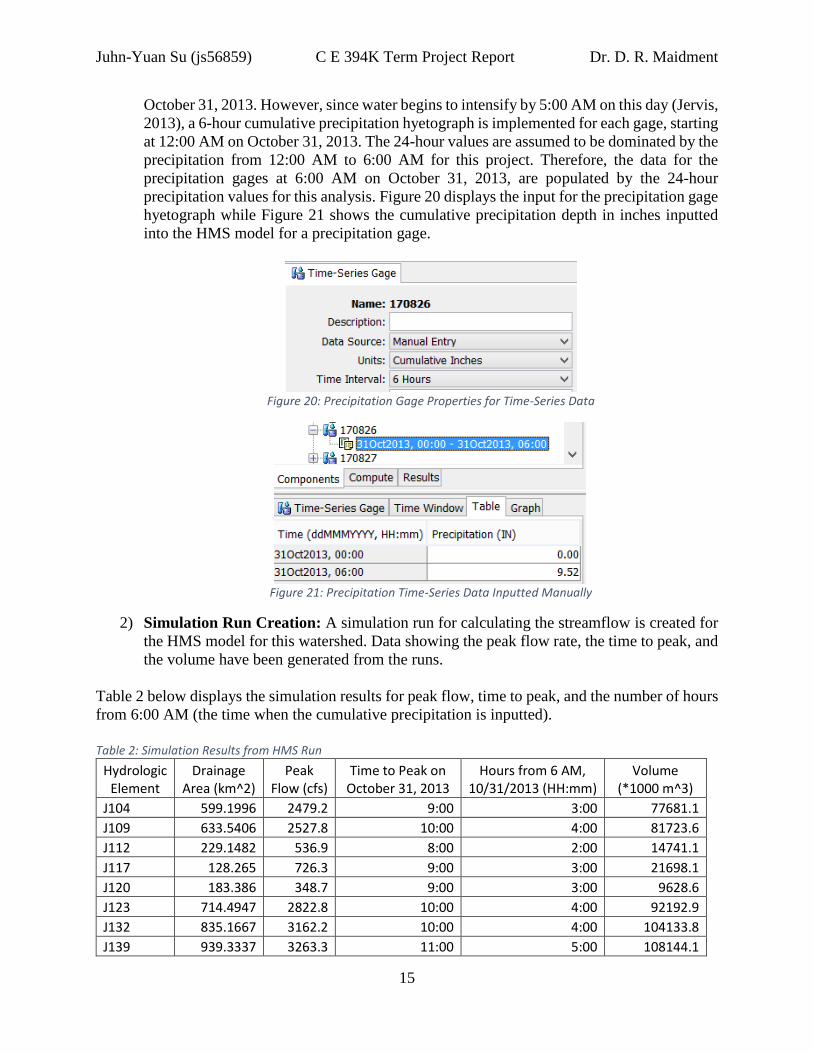
October 31, 2013. However, since water begins to intensify by 5:00 AM on this day (Jervis,

2013), a 6-hour cumulative precipitation hyetograph is implemented for each gage, starting

at 12:00 AM on October 31, 2013. The 24-hour values are assumed to be dominated by the

precipitation from 12:00 AM to 6:00 AM for this project. Therefore, the data for the

precipitation gages at 6:00 AM on October 31, 2013, are populated by the 24-hour

precipitation values for this analysis. Figure 20 displays the input for the precipitation gage

hyetograph while Figure 21 shows the cumulative precipitation depth in inches inputted

into the HMS model for a precipitation gage.

Figure 20: Precipitation Gage Properties for Time-Series Data

Figure 21: Precipitation Time-Series Data Inputted Manually

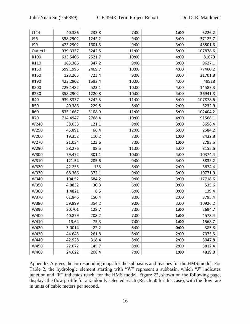
2) Simulation Run Creation: A simulation run for calculating the streamflow is created for

the HMS model for this watershed. Data showing the peak flow rate, the time to peak, and

the volume have been generated from the runs.

Table 2 below displays the simulation results for peak flow, time to peak, and the number of hours

from 6:00 AM (the time when the cumulative precipitation is inputted).

Table 2: Simulation Results from HMS Run

Hydrologic Element

Drainage Area (km^2)

Peak Flow (cfs)

Time to Peak on October 31, 2013

Hours from 6 AM, 10/31/2013 (HH:mm)

Volume (*1000 m^3)

J104 599.1996 2479.2 9:00 3:00 77681.1

J109 633.5406 2527.8 10:00 4:00 81723.6

J112 229.1482 536.9 8:00 2:00 14741.1

J117 128.265 726.3 9:00 3:00 21698.1

J120 183.386 348.7 9:00 3:00 9628.6

J123 714.4947 2822.8 10:00 4:00 92192.9

J132 835.1667 3162.2 10:00 4:00 104133.8

J139 939.3337 3263.3 11:00 5:00 108144.1


16

J144 40.386 233.8 7:00 1:00 5226.2

J96 358.2902 1242.2 9:00 3:00 37125.7

J99 423.2902 1601.5 9:00 3:00 48801.6

Outlet1 939.3337 3242.5 11:00 5:00 107878.6

R100 633.5406 2521.7 10:00 4:00 81679

R110 183.386 347.2 9:00 3:00 9627.1

R150 599.1996 2469.7 10:00 4:00 77460.2

R160 128.265 723.4 9:00 3:00 21701.8

R190 423.2902 1582.4 10:00 4:00 48518

R200 229.1482 523.1 10:00 4:00 14587.3

R230 358.2902 1220.8 10:00 4:00 36941.3

R40 939.3337 3242.5 11:00 5:00 107878.6

R50 40.386 229.8 8:00 2:00 5232.9

R60 835.1667 3108.9 11:00 5:00 102404.2

R70 714.4947 2768.4 10:00 4:00 91568.1

W240 38.033 121.1 9:00 3:00 3658.4

W250 45.891 66.4 12:00 6:00 2584.2

W260 19.352 110.2 7:00 1:00 2432.8

W270 21.034 123.6 7:00 1:00 2793.5

W290 58.276 88.5 11:00 5:00 3155.6

W300 79.472 301.1 10:00 4:00 10374.4

W310 121.54 205.6 9:00 3:00 5833.2

W320 42.253 133 8:00 2:00 3674.4

W330 68.366 372.1 9:00 3:00 10771.9

W340 104.52 584.2 9:00 3:00 17718.6

W350 4.8832 30.3 6:00 0:00 535.6

W360 1.4821 8.5 6:00 0:00 139.4

W370 61.846 150.4 8:00 2:00 3795.4

W380 59.899 354.2 9:00 3:00 10926.2

W390 20.701 128.7 7:00 1:00 2694.7

W400 40.879 208.2 7:00 1:00 4578.4

W410 13.64 75.3 7:00 1:00 1568.7

W420 3.0014 22.2 6:00 0:00 385.8

W430 44.643 261.8 8:00 2:00 7075.5

W440 42.928 318.4 8:00 2:00 8047.8

W450 22.072 145.7 8:00 2:00 3812.4

W460 24.622 208.4 7:00 1:00 4819.8

Appendix A gives the corresponding maps for the subbasins and reaches for the HMS model. For

Table 2, the hydrologic element starting with “W” represent a subbasin, which “J” indicates

junction and “R” indicates reach, for the HMS model. Figure 22, shown on the following page,

displays the flow profile for a randomly selected reach (Reach 50 for this case), with the flow rate

in units of cubic meters per second.


17

Figure 22: Flow Profile for Reach R50 in HMS

As shown in Table 2, some of the hydrologic elements exhibit peak flows at approximately 0 to 1

hour (indicated in bold) from 6:00 AM during the Halloween Flood simulation. Meanwhile, the

upstream elements seem to exhibit higher peak flows, indicating that many of the downstream

processes experience great water flows from upstream mechanisms. Therefore, if the precipitation

shown in Figure 16 (for the precipitation data for October 31, 2013) had all occurred within the 6-

hour period, then an emergency response may be necessary and done quickly to lower the risk of

this event from reoccurring.

Conclusion This project investigates the Halloween Flood that occurred along the Onion Creek Watershed in

2013. ArcHydro was employed to generate the drainage lines and sub-catchments for the

watershed while HEC-GeoHMS creates the feature classes and HMS files needed for the HMS

model. These files are imported into a HMS model, and precipitation data was manually entered

applying assumptions for this project that was at a small scale relative to a major project that

involves complex hydrologic modeling of a watershed. The project may be significantly improved


18

if more complex methods are employed for the HMS model simulation. For instance, instead of

using the SCS curve number method for analyzing losses for a subbasin, a more complex method,

such as not averaging the curve number over the subbasin or implementing groundwater

characteristics, may be employed. A similar change can also be applied for the Routing Method

for rivers, which a more complex model other than the Muskingum Cunge may be used to further

complicate the analysis. Finally, based on a simulation run, an emergency response seems needed

to react to the great peak flows to lower the risk of a similar event as the Halloween Flood from

reoccurring.

References Adam, J. C., & Lettenmaider, D. P. (2008). Application of New Precipitation and Reconstructed

Streamflow Products to Streamflow Trend Attribution in Northern Eurasia. Journal of

Climate, 21(8), 1807-1828.

Costache, R. (2014). Using GIS Techniques for Assessing Lag Time and Concentration Time in

Small River Basins- Case Study: Pecineaga River Basin, Romania. Geographia Technica,

9(1), 31-38.

Cronshey, R., McCuen, R. H., Miller, N., Rawls, W., Robbins, S., & Woodward, D. (1986). Urban

Hydrology for Small Watersheds. United States Department of Agriculture.

DHI. (2009). MIKE 11: A Modeling System for Rivers and Channels. Reference Manual.

Han, J. (2010). Streamflow Analysis using ArcGIS and HEC-GeoHMS. Project Report, Texas

A&M University, Zachary Department of Civil Engineering, College Station, TX.

Jasinski, L. E. (2010, June 15). Onion Creek, TX (Travis County). Retrieved from Texas State

Historical Association: A Digital Gateway to Texas History:

http://www.tshaonline.org/handbook/online/articles/hjo13

Jervis, R. (2013, November 7). Historic Flash Flood Leaves Devastation in Austin. Retrieved from

USA Today: http://www.usatoday.com/story/news/nation/2013/11/07/flash-flood-austin-

residents-killed-displaced/3459181/

Merwade, V. (2012). Creating SCS Curve Number Grid using HEC-GeoHMS. Purdue University,

Department of Civil Engineering.

Patterson, L. A., Lutz, B., & Doyle, M. W. (2012). Streamflow Changes in the South Atlantic,

United States during the Mid- and Late 20th Century. Journal of the American Water

Resources Association, 48(6), 1126-1138.

Rimmer, A., & Salingar, Y. (2006). Modeling Precipitation-Streamflow Processes in Karst Basin:

The Case of the Jordan River Sources, Israel. Journal of Hydrology, 331(3/4), 524-542.

Tobin, K. J., & Bennett, M. E. (2014). Impact of Model Complexity and Precipitation Data

Products on Modeled Streamflow. Journal of Hydroinformatics, 16(3), 588-599.

Yeh, H.-F., Lin, H.-I., Lee, S.-T., Chang, M.-H., Hsu, K.-C., & Lee, C.-H. (2014). GIS and SBF

for Estimating Groundwater Recharge of a Mountainous Basin in the Wu River Watershed,

Taiwan. Journal of Earth System Sciences, 123(3), 503-516.

A-1

Appendix A: HMS Maps This section displays the maps of the subbasins and reaches for the HMS model.

Map of Reaches Upstream Portion:

Middle Potion:

A-2

Downstream Portion:

Subbasin Map HMS Subbasin Labels

civil engineering 394k: topic 3 geographic information ... · juhn-yuan su (js56859) c e 394k term...

Documents