city research online · (shinozuka et al. (2000), cardone (2013)) demand parameters are used, while...
TRANSCRIPT

City, University of London Institutional Repository
Citation: Stefanidou, S.P. and Kappos, A. J. ORCID: 0000-0002-5566-5021 (2018). Bridge-specific fragility analysis: when is it really necessary?. Bulletin of Earthquake Engineering, doi: 10.1007/s10518-018-00525-9
This is the accepted version of the paper.
This version of the publication may differ from the final published version.
Permanent repository link: http://openaccess.city.ac.uk/id/eprint/21190/
Link to published version: http://dx.doi.org/10.1007/s10518-018-00525-9
Copyright and reuse: City Research Online aims to make research outputs of City, University of London available to a wider audience. Copyright and Moral Rights remain with the author(s) and/or copyright holders. URLs from City Research Online may be freely distributed and linked to.
City Research Online: http://openaccess.city.ac.uk/ [email protected]
City Research Online

Bridge-specific Fragility Analysis: When is it really necessary?
Sotiria P. Stefanidou1 and Andreas J. Kappos1,2
1 Department of Civil Engineering, Aristotle University
Thessaloniki, 54124, Greece
e-mail: [email protected]
2 Department of Civil Engineering, City, University of London
London EC1V OHB, UK
e-mail: [email protected]
Keywords: Bridges, Assessment, Bridge-Specific Fragility Curves, Limit State Thresholds,
Road network.
Abstract. In seismic assessment of bridges the research focus has recently shifted on the derivation of
bridge-specific fragility curves that account for the effect of different geometry, structural system,
component and soil properties, on the seismic behaviour. In this context, a new, component-based
methodology for the derivation of bridge-specific fragility curves has been recently proposed by the
authors, with a view to overcoming the inherent difficulties in assessing all bridges of a road network
and the drawbacks of existing methodologies, which use the same group of fragility curves for bridges
within the same typological class. The main objective of this paper is to critically assess the necessity
of bridge-specific fragility analysis, starting from the effect of structure-specific parameters on
component capacity (limit state thresholds), seismic demand, and fragility curves. The aforementioned
methodology is used to derive fragility curves for all bridges within an actual road network, with a view
to investigating the consistency of adopting generic fragility curves for bridges that fall within the same
class and quantifying the degree of over- or under- estimation of the probability of damage when generic
bridge classes are considered. Moreover, fragility curves for all representative bridges of the analysed
concrete bridge classes are presented to illustrate the differentiation in bridge fragility for varying
structural systems, bridge geometry, total bridge length and maximum pier height. Based on the above,
the relevance of bridge-specific fragility analysis is assessed, and pertinent conclusions are drawn.

1 INTRODUCTION
Reliability of road systems and their components, exposed to multiple natural hazards is at
the front line of engineering research during the last three decades, as possible damage to
critical components is strongly related to important direct and indirect economic losses. Bridges
are considered to be the most critical component of urban and interurban transport systems,
ensuring i.a. access to cities affected by a strong earthquake. In this context, numerous methods
have been developed for the assessment of seismic vulnerability of bridges, mainly in the form
of fragility curves.
Bridge fragility curves are essential for the estimation of the road or railway system’s
resilience, recovery planning, as well as pre- and post-earthquake retrofit prioritization. Both
analytical and empirical fragility curves were proposed by various research groups, the latter
being less frequent (e.g. Basoz & Kiremidjian, 1999), since earthquake damage data for
bridges is sparse. Analytical methodologies available in the literature can be classified based
on whether they consider multiple components (Mander & Basöz (1999), Nielson &
DesRoches (2007a), Moschonas et al. (2008), Zhang et al. (2008), Tsionis & Fardis (2012)) or
only the most critical one (piers) in fragility analysis (Banerjee & Shinozuka, 2007).
Classification can also be based on the procedure for estimation of component or system
capacity (limit state thresholds) and seismic demand (analysis method used), the uncertainty
treatment and the probabilistic model used (Table 1). Specifically, regarding component
capacity, either local (Avşar et al. (2011), Tsionis & Fardis (2012), Choi et al. (2004)) or global
(Shinozuka et al. (2000), Cardone (2013)) demand parameters are used, while quantification
of damage, namely the limit state thresholds, is commonly based on experimental results (Dutta
& Mander (1998), Berry & Eberhard (2003), HAZUS (2015)). Regarding the estimation of
seismic demand, different analysis methods have been put forward, namely inelastic static
(pushover) analysis (e.g. (Cardone et al. (2007), Moschonas et al. (2008)), elastic response
spectrum method (e.g. Mander & Basöz (1999), HAZUS (2015)) and nonlinear response-
history analysis (Mackie & Stojadinovic (2007), DesRoches et al. (2012)). The maximum
likelihood method (Shinozuka et al. 2000) and the probabilistic seismic demand model
(Nielson & Desroches 2007b) have been used for the derivation of fragility curves. The way
capacity and demand estimation is made in the frame of analytical methodologies for the
derivation of fragility curves is summarised in Table 1.
Bridge fragility curves are used in the assessment of seismic performance and losses in
bridge stocks providing valuable data for retrofit prioritisation, also in the frame of
transportation network recovery planning, strongly related to government investment and
decision-making. Therefore, the need for consistent and reliable fragility curves emerges. In a
practical context, these curves should be representative of a fairly small number of bridge
classes. The most common approach for deriving ‘generic’ fragility curves is to classify bridges
into different typological classes based on key structural and geometric characteristics like
structural system, number of spans, number of columns (single or multicolumn bents),
skewness, deck type, pier type and the pier-to-deck connection (Avşar et al. (2011), Moschonas
et al. (2008), Mander & Basöz (1999), Tsionis & Fardis (2012), DesRoches et al. (2012)) and
derive fragility curves for the generic bridge (representative of each class), to be used for the
assessment of the bridge stock, under the assumption that the seismic performance of bridges

within the same class is similar. The fragility curves proposed so far are based on analysis of
deterministically defined bridge models, accounting for varying geometric and material
properties within the probabilistic framework of fragility analysis. Furthermore, parametric
vulnerability curves are proposed in the literature (Elnashai et al. 2004) introducing generic
fragility functions based on analysis of bridges having different geometries and overstrength
ratios. The parametric approach is rather appealing, albeit oversimplified, since neither the
effect of different component properties on seismic demand and capacity, nor the effect of
different structural configuration on system fragility are captured.
Table 1: Capacity and demand estimation in analytical methodologies for the derivation of fragility curves
Research Group
Capacity Seismic Demand
Engineering
Demand
Parameter
Limit State thresholds Structural
model
Seismic
Input
Analysis
Method
1. Avşar et al. (2011)
Piers: φ
Beams: φ, Vu
Bearings: δ
[3 LS]
Piers: Priestley et al.,
(1996), Erduran & Yakut,
(2004)
Bearings: FHWA, (2006)
3D DM
25 accel.
(unscale
d)
NRHA
2. Banerjee &
Shinozuka (2007) Piers: μθ [5 LS] Dutta, (1999) 3D DM
3 × 20
accel.
NRHA &
CSM
3a. Cardone, Perrone
& Dolce (2007),
Cardone, Perrone, &
Sofia, 2011)
Cardone (2013)
Piers: δ
Bearings: δ
Abutments: δ
[3 LS]
Piers: δy & δu
Bearings: γ (%)
Konstantinidis et al. (2008)
Abutments: δgap & δu
MDOF→SD
OF, Adaptive
Pushover
Spectru
m
CSM
(adaptive)
3b.Cardone, Perrone,
& Sofia, 2011)
Piers: μφ, V
Bearings: δ, μδ
Abutments: F
[5 LS]
Piers: δy, 50% μδ, δu
Bearings: μδ
Abutments: Active &
Passive resistance
MDOF→SD
OF, Adaptive
Pushover
Spectru
m
CSM
(adaptive)
4. Choi et al. (2004)
Piers: μφ
Bearings: δ
[5 LS]
Piers: Dutta, (1999)
Bearings: Experiments 3D DM
100
synthetic
accel.
NRHA
5. Crowley et al.
(2011), Tsionis &
Fardis (2012)
Piers: θ
Bearings: δ
[2 LS]
Piers: θy & θu Biskinis &
Fardis, (2010a, b)
Bearings: Bousias et al.
2007
SDOF(Long),
Beam with
springs
(Trans)
EC8
elastic
spectrum
Equivalent
Static
6. De Felice &
Giannini (2010)
Piers: θ
[2 LS] θy & θu Metamodels
2 ×4
accel.
NRHA -
RSM
7. Dukes (2013)
Piers: μφ
Bearings: δ
Abutments: δ
[4 LS]
Piers: Dutta, (1999)
Bearings - Abutments:
Caltrans (2010)
Metamodels 3 ×40
accel.
NRHA -
RSM
8. Elnashai et al.
(2004) Piers: δ δy & δu (Pushover Curve) 3D DM
7accel.
(scaled) NRHA
9. Ghosh et al. (2013)
Piers: μφ
Bearings: δ
Abutments: δ
[4 LS]
Nielson & DesRoches
(2007b) Metamodels
24 accel.
(Wen&
Wu)
NRHA -
RSM

10. Hwang et al.,
(2001)
Piers: C/D factors
or μδ
[5 LS]
Piers: δy & δu 3D DM 100 acc.
synthetic NRHA
11. Karim &
Yamazaki
(2001,2003)
DI=(μδ+βμh)/μu
(Park-Ang)
[5 LS]
DI=0.00~1.00 SDOF 250
accel.
Nonlinear
Static/NRH
A
12. Mackie &
Stojadinovic (2004) Drift (%) Berry & Eberhard (2003) 3D DM 80 accel. NRHA
13. Mander & Basöz
(1999)
Piers: δ/h (%)
Bearings: δ
[5 LS]
Dutta, (1999) SDOF Elastic
spectrum CSM
14. Moschonas et al.
(2008)
Bridge: δ [5 LS]
[5 LS]
Piers: δy & δu (Pushover
curve)
Bearings: δ (γ %)
3D DM Elastic
spectrum CSM
15. Nielson &
DesRoches (2007a,
b)
Piers: μφ
Bearings: δ
Abutments: δ
[4 LS]
Piers: HAZUS (1997),
FHWA (2006)
Bearings, Abutments : Choi
(2004)
3D DM 48 accel.
(3 bins) NRHA
16. Ramanathan,
(2012)
Piers: μφ
Bearings: δ
Abutments: δ
[4 LS]
Piers: Berry & Eberhard
(2003),
Bearings, Abutments :
Caltrans (2010)
3D DM
320
accel. (4
bins)
NRHA
17. Shinozuka et al.
(2000)
Piers: μδ
[3 LS] 1.0 ≤ μδ ≤ 2.0 3D DM 80 accel. NRHA
18. Tavares et al.,
(2012)
Piers: μφ
Bearings: δ
Abutments: δ
[4 LS]
HAZUS (1997) 3D DM Syntheti
c Accel. NRHA
19. Yi et al. (2007) Piers: μφ
Bearings: δ
Choi (2004) 2D Model 60 accel. NRHA
20. Zhong et al. (2012) Piers: Drift (%)
Probabilistic model (closed
form relationship) 3D DM
Elastic
spectrum CSM
* 3D DM: 3D Detailed Model, NRHA: Nonlinear Response History Analysis CSM: Capacity Spectrum Method
It is clear that the accuracy and consistency of the assumption that fragility curves of a
generic bridge can be used for all bridges within the same class depend on the scope and size
of the classification scheme adopted. Moreover, it should be noted that component demand and
capacity vary and are related to component-specific properties, while bridge fragility was found
to be highly dependent on structure-specific parameters, like deck and pier geometry (Avşar et
al. (2011), Tavares et al. (2012), Elnashai et al. (2004)), structural system, which is related to
the topography and the construction method selected (Zhang et al., 2008), material and
geometric properties of components, as well as parameters related to the foundation soil and
the earthquake ground motion selection. The use of modification factors to account for the
effect of skewness and site conditions has been proposed (Mander & Basöz, 1999), an
appealing but rather oversimplified approach, as discussed in Dukes (2013). As an alternative,
the concept of bridge-specific fragility analysis has been put forward (Dukes (2013),
Stefanidou & Kappos (2015, 2017)), duly accounting for the effect of component-specific
properties on bridge fragility. However, the methodology proposed by Dukes (2013) focuses

on the correlation of component demand and structure-specific parameters, providing demand
models as a function of multiple design parameters in the frame of the ‘metamodeling’ concept,
not accounting for their effect on component capacity and limit state thresholds. On the other
hand, Stefanidou & Kappos (2017) proposed a holistic methodology for the estimation of
bridge-specific fragility curves providing empirical relationships for the estimation of
component-specific limit state thresholds, uncertainty treatment and demand estimation, the
amount of effort depending on the application scale (single bridge or bridge stocks).
The main objective of this paper is to put into context the relevance of bridge-specific
fragility analysis when an entire stock is addressed. Initially the effect of structure-specific
parameters on component capacity (limit state thresholds), seismic demand, and fragility
curves is established. The effect of pier properties on limit state thresholds is evaluated for
different concrete pier types, considering both local and global demand parameters. The
recently proposed (by the authors) methodology (Stefanidou & Kappos, 2017) is then applied
(using ad-hoc developed software) for the estimation of fragility curves for all bridges of an
actual road network, using the simplified approach, while uncertainty in demand estimation is
quantified based on the detailed approach entailing advanced analysis. Bridge-specific fragility
curves for all representative bridges of the different concrete bridge classes are presented, to
highlight the effect of structural system (different pier, deck and pier-to-deck connection types)
on bridge fragility. The effect of bridge geometry, namely total bridge length and maximum
pier height, on bridge fragility is evaluated through analysis of all bridges (and bridge classes)
of the road network under consideration. Subsequently, the consistency of adopting generic
fragility curves for bridges that fall within the same category is assessed, by quantifying the
degree of over- or under- estimation of the probability of damage when generic bridge classes
are used. The conclusions of this study refer to the concrete bridge stock studied (described in
detail in §4.2.1), which is typical of Southern Europe motorways. Nevertheless, the proposed
methodology for bridge-specific fragility analysis has a broad application range and could be
used for the seismic assessment of any other bridge stock.
2 METHODOLOGY FOR DERIVING BRIDGE-SPECIFIC FRAGILITY CURVES
The methodology proposed by the authors for the derivation of bridge-specific fragility
curves and the successive steps for its implementation are described in detail elsewhere
(Stefanidou & Kappos, 2017). It is noted that a key aspect of the methodology is that it does
not depend on the structural system and bridge properties, minimising the need for
classification to typological classes. The methodology, outlined in the flowchart of Fig.1, is
component-based and entails closed-form relationships for defining component-specific limit
state thresholds (component database) and two alternatives for the calculation of seismic
demand based on analysis of a detailed or simplified bridge model, depending on whether a
single bridge or a bridge stock is addressed. Obviously, the question of whether bridge-specific
analysis is really necessary arises when entire stocks are analysed, hence the basic principles
for the estimation of component capacity (database development) and seismic demand briefly
described in the remainder of this section refer to this case; more details of both versions of the
methodology are found in Stefanidou & Kappos (2017).

Fig. 1 – Flowchart of the component-based methodology for the derivation of bridge-specific fragility
curves applied to a population of bridges
2.1 Bridge capacity
As depicted in Table 1, different global or local demand parameters (EDP) are utilised in
existing methodologies for the quantification of component damage, while threshold values are
in most cases based on experimental results. Whenever analytical estimation of limit state
thresholds is proposed, component-specific analysis is required, rendering the methodology
case-dependent and increasing the computational cost.
In the frame of the proposed methodology, bridge piers, abutments and bearings are
considered as critical components affecting the system’s seismic performance, and limit state
thresholds for four limit states are explicitly defined based on inelastic analysis results and/or
experimental data, depending on the component examined. The milestone of the proposed
methodology as far as capacity estimation is concerned, is that the user can define component
limit state thresholds considering all different component properties that may affect inelastic
behaviour, without performing inelastic analysis for each component. To this end, a database
of different components has been developed, based on multiple parametric inelastic analyses
(considering different possible failure modes) to derive limit state thresholds. Based on
regression analysis of the results, closed-form relationships were derived for limit state
thresholds, based on various parameters affecting capacity of different component types.
Hence, irrespectively of the procedure followed for fragility estimation, a reliable methodology
for limit state threshold (capacity) estimation is provided.
Regarding the component which is usually the most critical for the seismic response, namely
bridge piers, the procedure followed for the development of the database is presented in Fig. 2.
The steps for the compilation of the database are:

(a) Consideration of different concrete pier types, encompassing practically all common
types found in a European bridge stock. Cylindrical, hollow cylindrical, rectangular,
hollow rectangular and wall-type piers are considered herein. It should be mentioned
that hollow rectangular and wall piers are commonly designed to remain elastic
(especially in bridges with pier-to-deck connection through bearings), nevertheless their
inelastic behaviour was studied to quantify all limit state thresholds.
Fig. 2 – Procedure for development of database for bridge piers
(details provided in Stefanidou & Kappos (2017))
(b) Consideration of pier cross section parameters, namely dimensions, longitudinal and
transverse reinforcement ratio, normalised axial force, and material properties. Section
analyses are performed for all relevant combinations of parameters considering confined
and unconfined concrete material laws. Specifically, for confined concrete the Mander
et al. (1988) model is used for cylindrical sections, the Priestley & Ranzo (2000) model
for hollow cylindrical sections, and the Kappos (1991) model for rectangular, hollow
rectangular, and wall sections. Parametrically defined input cross section files are set up
and multiple section analyses are performed using the software AnySection
(Papanikolaou, 2012). Pier damage is initially defined at cross section level, using local
demand parameters (section curvature, φ), related to experimentally estimated damage
(e.g. crack widths) via section analysis, therefore limit state thresholds in curvature
(local) terms (Table 2) are defined within this step.
(c) Consideration of a sufficiently broad range of heights for each pier section type and
parametric setup of an inelastic cantilever model in order to perform pushover analysis
and define limit state thresholds in terms of a global demand parameter (displacement
of control point). Plastic hinge formation is considered at the cantilever base (lumped
plasticity model), whereas the M-φ curve, calculated at step (b), is used as input.
Inelastic static analysis is performed for all sections considered (strong and weak section
direction analysed separately) paired with all different pier heights, using a Matlab-
based code developed for the setup of input files, and Opensees (McKeena & Fenves,
2015) for inelastic static analysis. Limit state thresholds in global terms (displacement
of control point for limit states 1 to 4) are correlated to local ones (curvature for limit
states 1 to 4), using the results of inelastic pushover analysis, additionally considering
P-delta effects.
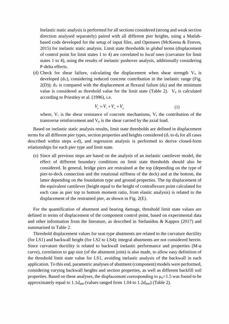
(d) Check for shear failure, calculating the displacement when shear strength Vu is
developed (dV), considering reduced concrete contribution in the inelastic range (Fig.
2(D)); dV is compared with the displacement at flexural failure (dfl) and the minimum
value is considered as threshold value for the limit state (Table 2). Vu is calculated
according to Priestley et al. (1996), i.e.
u c w pV V V V
(1)
where, Vc is the shear resistance of concrete mechanisms, Vs the contribution of the
transverse reinforcement and Vp is the shear carried by the axial load.
Based on inelastic static analysis results, limit state thresholds are defined in displacement
terms for all different pier types, section properties and heights considered (d1 to d4 for all cases
described within steps a-d), and regression analysis is performed to derive closed-form
relationships for each pier type and limit state.
(e) Since all previous steps are based on the analysis of an inelastic cantilever model, the
effect of different boundary conditions on limit state thresholds should also be
considered. In general, bridge piers are restrained at the top (depending on the type of
pier-to-deck connection and the rotational stiffness of the deck) and at the bottom, the
latter depending on the foundation type and ground properties. The tip displacement of
the equivalent cantilever (height equal to the height of contraflexure point calculated for
each case as pier top to bottom moment ratio, from elastic analysis) is related to the
displacement of the restrained pier, as shown in Fig. 2(E).
For the quantification of abutment and bearing damage, threshold limit state values are
defined in terms of displacement of the component control point, based on experimental data
and other information from the literature, as described in Stefanidou & Kappos (2017) and
summarised in Table 2.
Threshold displacement values for seat-type abutments are related to the curvature ductility
(for LS1) and backwall height (for LS2 to LS4); integral abutments are not considered herein.
Since curvature ductility is related to backwall inelastic performance and properties (M-φ
curve), correlation to gap size (of the abutment joint) is also made, to allow easy definition of
the threshold limit state value for LS1, avoiding inelastic analysis of the backwall in each
application. To this end, parametric analyses of abutment (component) models were performed,
considering varying backwall heights and section properties, as well as different backfill soil
properties. Based on these analyses, the displacement corresponding to μφ=1.5 was found to be
approximately equal to 1.1dgap (values ranged from 1.04 to 1.2dgap) (Table 2).
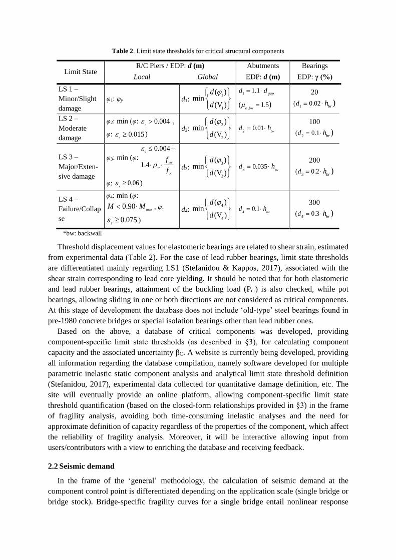
Table 2. Limit state thresholds for critical structural components
Limit State R/C Piers / EDP: d (m) Abutments Bearings
Local Global EDP: d (m) EDP: γ (%)
LS 1 –
Minor/Slight
damage
φ1: φy d1: 1
1
( )min
(V )
d
d
11.1
gapd d
,bw( 1.5)
20
1( 0.02 )
brd h
LS 2 –
Moderate
damage
φ2: min (φ: 0.004c ,
φ: 0.015s )
d2: 2
2
( )min
(V )
d
d
2
0.01bw
d h 100
2( 0.1 )
brd h
LS 3 –
Major/Exten-
sive damage
φ3: min (φ:
0.004
1.4
c
yw
w
cc
f
f
φ: 0.06s )
d3: 3
3
( )min
(V )
d
d
3
0.035bw
d h 200
3( 0.2 )
brd h
LS 4 –
Failure/Collap
se
φ4: min (φ:
max0.90M M , φ:
0.075s )
d4: 4
4
( )min
(V )
d
d
4
0.1bw
d h 300
4( 0.3 )
brd h
*bw: backwall
Threshold displacement values for elastomeric bearings are related to shear strain, estimated
from experimental data (Table 2). For the case of lead rubber bearings, limit state thresholds
are differentiated mainly regarding LS1 (Stefanidou & Kappos, 2017), associated with the
shear strain corresponding to lead core yielding. It should be noted that for both elastomeric
and lead rubber bearings, attainment of the buckling load (Pcr) is also checked, while pot
bearings, allowing sliding in one or both directions are not considered as critical components.
At this stage of development the database does not include ‘old-type’ steel bearings found in
pre-1980 concrete bridges or special isolation bearings other than lead rubber ones.
Based on the above, a database of critical components was developed, providing
component-specific limit state thresholds (as described in §3), for calculating component
capacity and the associated uncertainty βC. A website is currently being developed, providing
all information regarding the database compilation, namely software developed for multiple
parametric inelastic static component analysis and analytical limit state threshold definition
(Stefanidou, 2017), experimental data collected for quantitative damage definition, etc. The
site will eventually provide an online platform, allowing component-specific limit state
threshold quantification (based on the closed-form relationships provided in §3) in the frame
of fragility analysis, avoiding both time-consuming inelastic analyses and the need for
approximate definition of capacity regardless of the properties of the component, which affect
the reliability of fragility analysis. Moreover, it will be interactive allowing input from
users/contributors with a view to enriching the database and receiving feedback.
2.2 Seismic demand
In the frame of the ‘general’ methodology, the calculation of seismic demand at the
component control point is differentiated depending on the application scale (single bridge or
bridge stock). Bridge-specific fragility curves for a single bridge entail nonlinear response

history analysis of a detailed inelastic model, using an enhanced IDA procedure described in
Stefanidou & Kappos (2017) (IDA combined with multiple stripe analysis), in order to estimate
seismic demand at component control points for different levels of earthquake intensity.
Uncertainty in seismic demand (logarithmic standard deviation βD) is calculated for each
critical component (with random properties), also accounting for record-to-record variability.
Since the application of the methodology to bridge stocks for the derivation of bridge-specific
fragility curves is computationally demanding, the procedure proposed for bridge stock
analysis (described in Stefanidou & Kappos (2017)) is applied, and response spectrum analysis
of a simplified elastic model using the Eurocode 8 spectrum for varying levels of earthquake
intensity is invoked (scaling PGA, typically from 0.1g to 1g) to estimate seismic demand at
component control points; the evolution of damage with earthquake intensity is plotted for each
component considered (mean value). Bridge-specific fragility curves are plotted assuming
lognormal distribution, while uncertainty in seismic demand (βD), calculated for generic
bridges representative of a specific bridge class according to the classification system proposed
by Moschonas et al. (2008), is used as dispersion value. It is clear that in practical fragility
analysis it is not feasible (nor desirable) to estimate uncertainty through Monte Carlo analysis
(even with reduced sampling) of each individual bridge; β values should inevitably come from
a classification-based approach.
Fig. 3 – Software for bridge-specific fragility curves (input data – cases of open/closed gap)
For bridge stock analysis, a Matlab-based software is developed for the derivation of
bridge-specific fragility curves. The software is based on a generic (parametrically defined),
simplified 3D bridge model created using the OpenSees platform (McKeena & Fenves, 2015)
according to bridge-specific, user-defined properties. The methodology described in
Stefanidou & Kappos (2017) for single bridge analysis is embedded in the software;
component-specific limit state thresholds are calculated based on user-defined properties and
multiple response spectrum analyses for varying levels of earthquake intensity are performed
for demand estimation. Different boundary conditions at abutments are considered for the case
of open and closed gap, while fragility curves are automatically derived and plotted for each
component, separately for the longitudinal and transverse directions. Bridge-specific fragility
curves for the entire bridge are calculated and plotted, under the assumption of series
Deck
Kbear
Gap Open
Kabtm
Deck
Deck
Gap Closed
Kbear
Kabtm
Deck

connection between components (lower bound), except for LS4, where piers or abutments are
considered as critical components. Detailed description of the software developed can be found
elsewhere (Stefanidou, 2017).
3 SEISMIC CAPACITY ASSESSMENT (DATABASE FOR LIMIT STATE
THRESHOLDS)
The first step to gain insight into the relevance of bridge-specific fragility analysis, is to
evaluate the effect of varying properties on component capacity, which is related to the limit
state thresholds, or, in other words, to component damage for the limit states considered. To
this end, different pier types and properties are considered, in the frame of the methodology
proposed by Stefanidou & Kappos (2017), with a view to developing a database encompassing
practically all common concrete pier types found in a bridge stock. The effect of varying pier
properties on limit state thresholds is evaluated herein for different pier types and the results,
considering both local and global demand parameters, are discussed.
A broad range of different section properties, namely dimensions, longitudinal and
transverse reinforcement ratio, normalised axial force and material properties are considered,
and section analysis is performed as described in §2.1(b). Damage is initially quantified using
material strain values, namely εc and εs corresponding to experimentally observed crack widths,
and moment corresponding to loss of bearing capacity for limit state 4 (post-peak M=0.9∙Mmax).
Based on cross section analysis, moment-curvature curves are calculated (and bilinearised) and
curvature values corresponding to the aforementioned material strains are defined. Hence,
damage is initially defined in curvature terms (local EDPs φ1, φ2, φ3, φ4), and M-φ curves as
well as effective stiffnesses EIeff (My/φy), needed for pushover analysis, are defined.
Section analysis results for all possible parameter combinations (nearly 8000 section
analyses for each pier type considering weak and strong section axes separately), are obtained
for each pier type and regression analysis is performed. As an example, closed-form
relationships for φy, φu and Μy, Mu are presented in Table 3 for cylindrical piers; relevant
relationships are available for all different pier types, however a detailed presentation is beyond
the scope of this paper (it will be made available on the aforementioned website).
Table 3. Closed-form relationships for the estimation of moment vs curvature for cylindrical piers
-5.716 -0.734 -0.017 +0.309 +0.089
-2.331 -0.602 -0.582 -0.049 +0.602
-0.369 -0.633 +0.225 +0.551 +0.053
-0.269 -0.645 +0.217 +0.559 +0.054
The effect of varying cross section parameters on local demand parameters (φ or μφ values)
is depicted in Figures 4 and 5 for cylindrical piers and Fig. 6 for different pier types,
0 1 2 3 4( )exp[ lnln / ( ) ln ln ]yc l wvD f f
3
0 1 2 3 4( ) ln( ) ln2 exp[ ln / ln ]cd c y l wM R f f f v
0
1
2 3
4
y
u
yM
uM

highlighting the over- or under-estimation of threshold values in case that a uniform value,
irrespective of section properties, is considered.
D=2.0 (m), fc= 33 (MPa), fy= 550 (MPa), v=0.20 D=2.0 (m), fc= 33 (MPa), fy= 550 (MPa), v=0.20
Fig. 4 – Effect of longitudinal and transverse reinforcement ratio on yield (left) and ultimate (right) curvature of
cylindrical sections
D=2.0 (m), fc= 33 (MPa), ρw= 0.010, v=0.20 D=2.0 (m), ρl= 0.015, ρw= 0.010, v=0.20
Fig. 5 – Effect of steel strength and longitudinal reinforcement ratio on curvature ductility (left) and steel and
concrete strength on ultimate curvature (right) of cylindrical sections
As shown in Fig. 4, yield curvature increases for increasing longitudinal reinforcement ratio
(ρl), while the effect of transverse reinforcement ratio (ρw) is negligible. On the contrary,
ultimate curvature is highly affected (increased for increasing transverse reinforcement), due
to the relevant increase in ultimate concrete strain (εcu) caused by confinement. The effect of
concrete and steel strength on ultimate curvature is depicted in Fig. 5(right). Based on the
above, curvature ductility decreases for increasing longitudinal reinforcement ratio (μφ=φu/φy
– Fig. 5(left)), while this effect is more pronounced for ρl >0.01.
It is evident from Fig. 6 that an increase in compressive axial load (νd) results in decrease of
curvature ductility, due to the associated increase in compression zone depth (xu). Moreover,
as shown in Fig. 6, the effect of transverse reinforcement on available curvature ductility is
more pronounced for lower values of compressive axial load.
0.005
0.01
0.015
0
0.01
0.02
0.031.5
2
2.5
3
3.5x 10
-3
w
y -
l -
w
l
y
0.005
0.01
0.015
0
0.01
0.02
0.030.02
0.03
0.04
0.05
0.06
w
u -
l -
w
l
u
0
0.01
0.02
0.03 200
300
400
500
60010
20
30
fy
- f
y -
l
l
200300
400500
600
20
30
40
500.02
0.03
0.04
0.05
fy
u - f
c - f
y
fc
u
Cylindrical Piers Hollow Rectangular Piers Rectangular Piers
D=2.0 (m, fc= 33 (MPa), fy= 550 (MPa),
v=0.20
H=6.0 (m), B=3.0 (m), t=0.6 (m), fc= 33
(MPa), fy= 550 (MPa), v=0.20
H=0.8 (m) , B=1.0 (m) , fc= 33 (MPa), fy=
550 (MPa), v=0.20
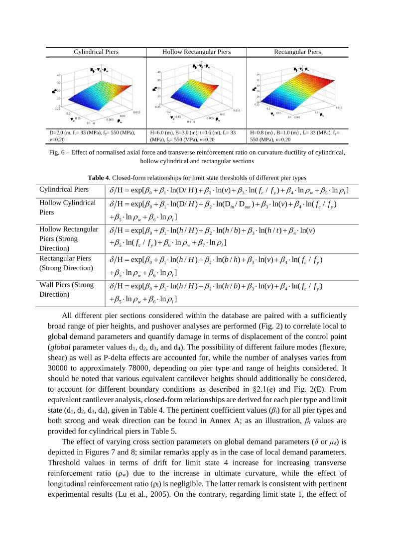
Fig. 6 – Effect of normalised axial force and transverse reinforcement ratio on curvature ductility of cylindrical,
hollow cylindrical and rectangular sections
Table 4. Closed-form relationships for limit state thresholds of different pier types
Cylindrical Piers 0 1 2 3 4 5(D/ ) ln(exp[ ) ( ) lnln l l ]n / ny w lc fH v f
Hollow Cylindrical
Piers 0 1 2 3 4
5 6
(D/ ) (D / D ) ln( ) ( )exp[ ln ln ln
ln ln ]
/in out y
w l
cH v f f
Hollow Rectangular
Piers (Strong
Direction)
0 1 2 3 4
5 6 7
exp[ ln ln( / ) ( / ) ( / ) ln( )
( ) ln ln
ln
/ ]ln y wc l
h H h b h t
f f
v
Rectangular Piers
(Strong Direction) 0 1 2 3 4
5 6
( / ) ( / ) lexp[ ln ln lnn( ) ( )
l
/
n ln ]
y
w
c
l
fh h v fH b
Wall Piers (Strong
Direction) 0 1 2 3 4
5 6
( / ) ( / ) lexp[ ln ln lnn( ) ( )
l
/
n ln ]
y
w
c
l
fh b v fH h
All different pier sections considered within the database are paired with a sufficiently
broad range of pier heights, and pushover analyses are performed (Fig. 2) to correlate local to
global demand parameters and quantify damage in terms of displacement of the control point
(global parameter values d1, d2, d3, and d4). The possibility of different failure modes (flexure,
shear) as well as P-delta effects are accounted for, while the number of analyses varies from
30000 to approximately 78000, depending on pier type and range of heights considered. It
should be noted that various equivalent cantilever heights should additionally be considered,
to account for different boundary conditions as described in §2.1(e) and Fig. 2(E). From
equivalent cantilever analysis, closed-form relationships are derived for each pier type and limit
state (d1, d2, d3, d4), given in Table 4. The pertinent coefficient values (βi) for all pier types and
both strong and weak direction can be found in Annex A; as an illustration, βi values are
provided for cylindrical piers in Table 5.
The effect of varying cross section parameters on global demand parameters (δ or μδ) is
depicted in Figures 7 and 8; similar remarks apply as in the case of local demand parameters.
Threshold values in terms of drift for limit state 4 increase for increasing transverse
reinforcement ratio (ρw) due to the increase in ultimate curvature, while the effect of
longitudinal reinforcement ratio (ρl) is negligible. The latter remark is consistent with pertinent
experimental results (Lu et al., 2005). On the contrary, regarding limit state 1, the effect of
0
0.005
0.01
0.015
0.1
0.15
0.2
0.250
10
20
30
40
w
-
d -
w
d
0
0.005
0.01
0.015
0.1
0.15
0.2
0.250
10
20
30
40
w
-
d -
w
d
0.005
0.01
0.015
0.1
0.15
0.2
0.2524
26
28
30
32
34
w
-
d -
w
d
longitudinal reinforcement ratio (ρl) on drift value is more significant, as this affects the yield
curvature.
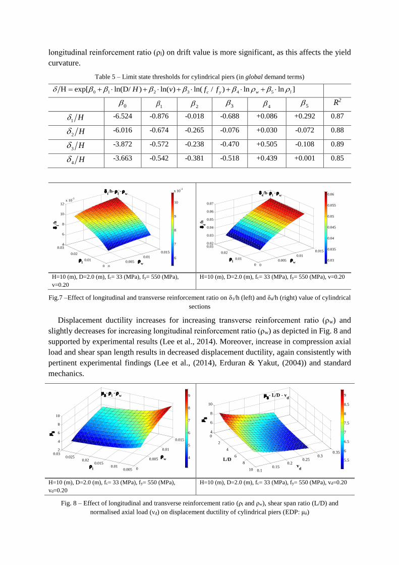
Table 5 – Limit state thresholds for cylindrical piers (in global demand terms)
0 1 2 3 4 5(D/ ) ln(exp[ ) ( ) lnln l l ]n / ny w lc fH v f
0
1
2 3
4
5 R2
1H -6.524 -0.876 -0.018 -0.688 +0.086 +0.292 0.87
2H -6.016 -0.674 -0.265 -0.076 +0.030 -0.072 0.88
3H -3.872 -0.572 -0.238 -0.470 +0.505 -0.108 0.89
4H -3.663 -0.542 -0.381 -0.518 +0.439 +0.001 0.85
H=10 (m), D=2.0 (m), fc= 33 (MPa), fy= 550 (MPa),
v=0.20
H=10 (m), D=2.0 (m), fc= 33 (MPa), fy= 550 (MPa), v=0.20
Fig.7 –Effect of longitudinal and transverse reinforcement ratio on δ1/h (left) and δ4/h (right) value of cylindrical
sections
Displacement ductility increases for increasing transverse reinforcement ratio (ρw) and
slightly decreases for increasing longitudinal reinforcement ratio (ρw) as depicted in Fig. 8 and
supported by experimental results (Lee et al., 2014). Moreover, increase in compression axial
load and shear span length results in decreased displacement ductility, again consistently with
pertinent experimental findings (Lee et al., (2014), Erduran & Yakut, (2004)) and standard
mechanics.
H=10 (m), D=2.0 (m), fc= 33 (MPa), fy= 550 (MPa),
vd=0.20
H=10 (m), D=2.0 (m), fc= 33 (MPa), fy= 550 (MPa), vd=0.20
Fig. 8 – Effect of longitudinal and transverse reinforcement ratio (ρl and ρw), shear span ratio (L/D) and
normalised axial load (νd) on displacement ductility of cylindrical piers (EDP: μδ)
0
0.005
0.01
0.015
0
0.01
0.02
0.034
6
8
10
12x 10
-3
w
1/h-
l -
w
l
1/h
6
7
8
9
10
x 10-3
0
0.005
0.01
0.015
0
0.01
0.02
0.030.02
0.03
0.04
0.05
0.06
0.07
w
4/h-
l -
w
l
4/h
0.03
0.035
0.04
0.045
0.05
0.055
0.06
0
0.005
0.01
0.015
0.0050.01
0.0150.02
0.0250.03
2
4
6
8
10
w
-
l -
w
l
4
5
6
7
8
9
0
2
4
6
8
10 0.10.15
0.20.25
0.30.35
4
6
8
10
vd
- L/D - v
d
L/D
5.5
6
6.5
7
7.5
8
8.5
9
4 SEISMIC DEMAND ASSESSMENT (UNCERTAINTY IN SEISMIC DEMAND)
In bridge fragility analysis the seismic demand at component control points (see section 2)
has to be defined. The methodology proposed for bridge-specific fragility analysis entails two
alternative approaches for demand estimation, related to whether a single bridge or a bridge
stock is addressed. Within bridge stock analysis (simplified approach), component demand is
calculated based on elastic response spectrum analysis results of the simplified model
(described in Fig. 3), while a reliable estimation of uncertainty in seismic demand (βD) is based
on single bridge analysis (detailed approach). To this end a classification-based procedure is
used to quantify uncertainty in seismic demand for the representative bridges of the most
frequent classes based on nonlinear response history analysis results of the inelastic model and
eventually provide βD values for bridge-specific fragility analysis of bridge stocks using the
simplified model and elastic response spectrum analysis. This is the most refined method for
βD quantification, based on analysis results, rather than literature recommendations (many past
studied relied on HAZUS, 2015).
The bridge inventory considered herein is part of Egnatia Motorway in Greece, a typical
modern motorway in Southern Europe. Bridge-specific fragility curves for all bridges of the
road network are provided in a following section (§5) based on the simplified approach, while
the variation of dispersion value βD (uncertainty in demand) within different bridge classes
(and critical components) is discussed herein, based on the detailed approach and inelastic
dynamic analysis of refined bridge models. Representative bridges of three common classes in
the stock are considered and the effect of structural configuration and component-specific
properties on uncertainty in demand is evaluated at component and system level.
4.1 Classification of bridge stock
The bridges of the inventory, classified into categories according to an enhanced version of
the classification scheme proposed by Moschonas et al. (2009) are summarised in Table 6; the
scheme is tailored to the typologies common in medium and high seismicity areas of Europe.
A code number (X1X2X3) is defined for each bridge according to the pier, deck, and pier-to-
deck connection, type. It is noted that, in principle, classification of bridges is not necessary
for the application of the methodology proposed for the derivation of bridge-specific fragility
curves. However, for reasons of practicality (explicit quantification of uncertainty is time
consuming), bridges that fall within the same category are assumed to have the same
uncertainty in demand; hence the need for classification.
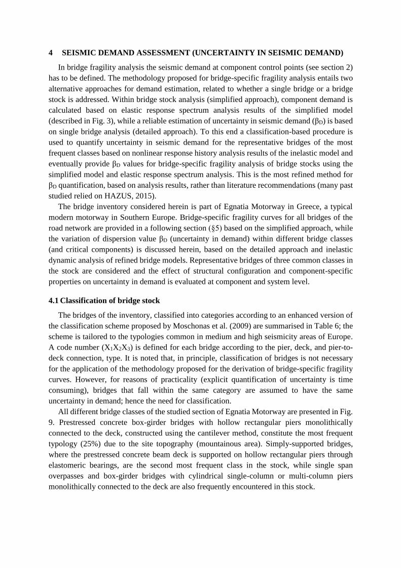
All different bridge classes of the studied section of Egnatia Motorway are presented in Fig.
9. Prestressed concrete box-girder bridges with hollow rectangular piers monolithically
connected to the deck, constructed using the cantilever method, constitute the most frequent
typology (25%) due to the site topography (mountainous area). Simply-supported bridges,
where the prestressed concrete beam deck is supported on hollow rectangular piers through
elastomeric bearings, are the second most frequent class in the stock, while single span
overpasses and box-girder bridges with cylindrical single-column or multi-column piers
monolithically connected to the deck are also frequently encountered in this stock.
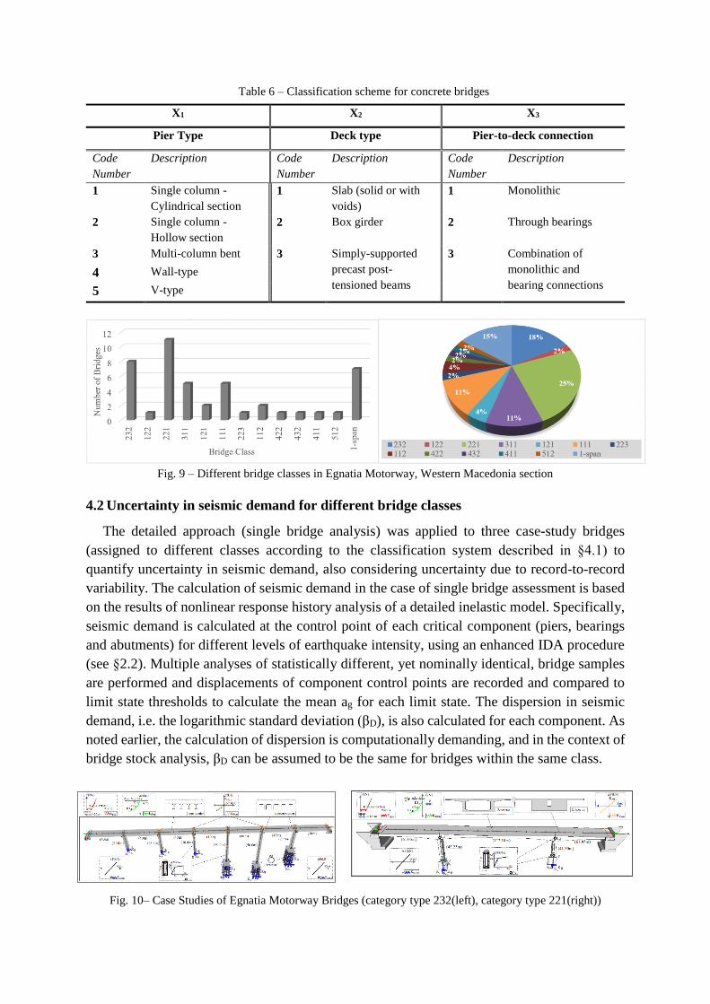
Table 6 – Classification scheme for concrete bridges
X1 X2 X3
Pier Type Deck type Pier-to-deck connection
Code
Number
Description Code
Number
Description Code
Number
Description
1 Single column -
Cylindrical section
1 Slab (solid or with
voids)
1 Monolithic
2 Single column -
Hollow section
2 Box girder 2 Through bearings
3 Multi-column bent 3 Simply-supported
precast post-
tensioned beams
3 Combination of
monolithic and
bearing connections 4 Wall-type
5 V-type
Fig. 9 – Different bridge classes in Egnatia Motorway, Western Macedonia section
4.2 Uncertainty in seismic demand for different bridge classes
The detailed approach (single bridge analysis) was applied to three case-study bridges
(assigned to different classes according to the classification system described in §4.1) to
quantify uncertainty in seismic demand, also considering uncertainty due to record-to-record
variability. The calculation of seismic demand in the case of single bridge assessment is based
on the results of nonlinear response history analysis of a detailed inelastic model. Specifically,
seismic demand is calculated at the control point of each critical component (piers, bearings
and abutments) for different levels of earthquake intensity, using an enhanced IDA procedure
(see §2.2). Multiple analyses of statistically different, yet nominally identical, bridge samples
are performed and displacements of component control points are recorded and compared to
limit state thresholds to calculate the mean ag for each limit state. The dispersion in seismic
demand, i.e. the logarithmic standard deviation (βD), is also calculated for each component. As
noted earlier, the calculation of dispersion is computationally demanding, and in the context of
bridge stock analysis, βD can be assumed to be the same for bridges within the same class.
Fig. 10– Case Studies of Egnatia Motorway Bridges (category type 232(left), category type 221(right))
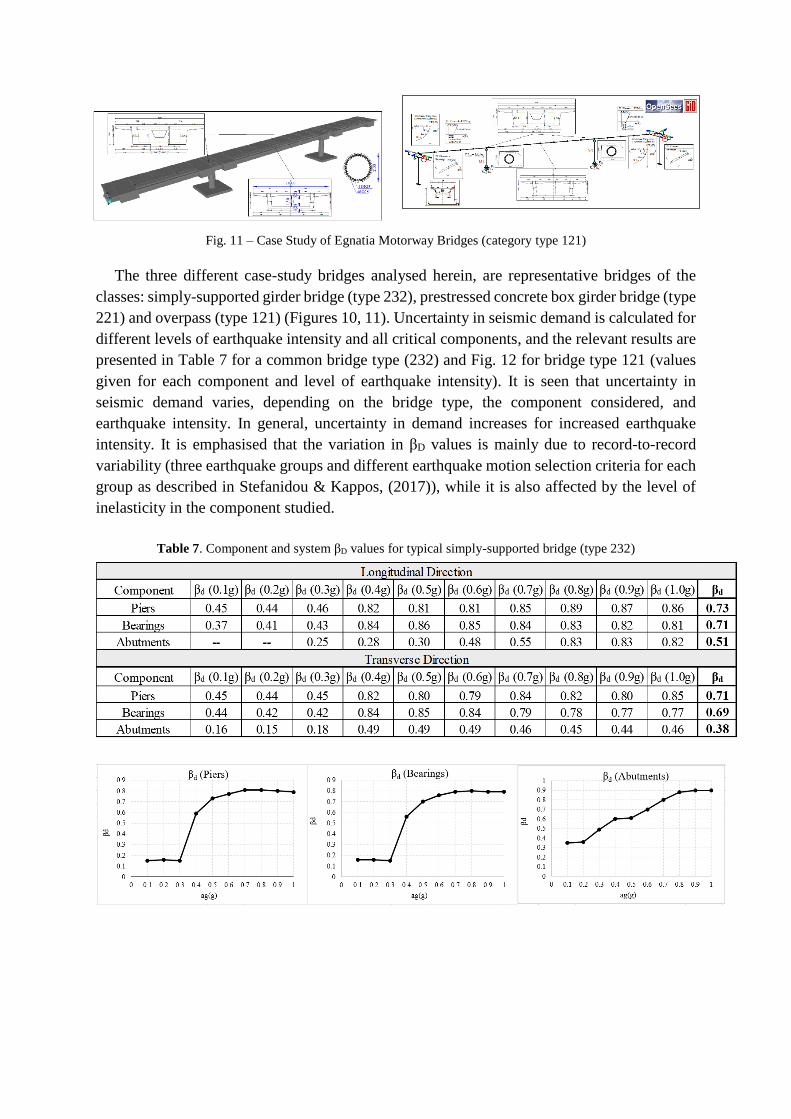
Fig. 11 – Case Study of Egnatia Motorway Bridges (category type 121)
The three different case-study bridges analysed herein, are representative bridges of the
classes: simply-supported girder bridge (type 232), prestressed concrete box girder bridge (type
221) and overpass (type 121) (Figures 10, 11). Uncertainty in seismic demand is calculated for
different levels of earthquake intensity and all critical components, and the relevant results are
presented in Table 7 for a common bridge type (232) and Fig. 12 for bridge type 121 (values
given for each component and level of earthquake intensity). It is seen that uncertainty in
seismic demand varies, depending on the bridge type, the component considered, and
earthquake intensity. In general, uncertainty in demand increases for increased earthquake
intensity. It is emphasised that the variation in βD values is mainly due to record-to-record
variability (three earthquake groups and different earthquake motion selection criteria for each
group as described in Stefanidou & Kappos, (2017)), while it is also affected by the level of
inelasticity in the component studied.
Table 7. Component and system βD values for typical simply-supported bridge (type 232)

Fig. 12 – Component and system βD values for typical overpass (type 121)
Uncertainty in seismic demand, i.e. βD values for all critical components and bridge types
considered, are summarised in Table 8 based on bridge-specific fragility analysis of the
representative bridge in each class. As shown in Table 8, the βD value for the system is related
to the most critical component (varying with the structural system), while the assumption of a
uniform (average) βD value for the longitudinal and transverse direction in each bridge class
appears to be consistent, since differences are mainly up to 15%. Nevertheless, it should be
noted that this consistency should be related to the consideration of a uniform βD value for the
system at all levels of earthquake intensity; note that using a single value for all curves is not
only simpler but also prevents the not uncommon situation of intersecting fragility curves (due
to the different βD), which lacks physical meaning and leads to inconsistent results.
Table 8. Component and system βD values for some common bridge types
Bridge
Class
βD
Longitudinal Direction Transverse Direction
Piers Bearings Abutments Bridge
System Piers Bearings Abutments Bridge
System
#232 0.88 0.73 0.67 0.73 0.86 0.71 0.59 0.71
#221 0.74 0.62 0.86 0.74 0.80 0.82 0.77 0.80
#121 0.76 0.59 0.79 0.76 0.81 0.64 0.69 0.81
4.3 Total Uncertainty for different bridge classes of a bridge stock
The fragility curve for the bridge system should be drawn for the βtot value of the most
critical component under the series connection assumption; the latter is typically the bearings
in simply-supported bridges, and the piers in monolithic bridges (Nielson, 2005). As discussed
in Stefanidou & Kappos (2017), the total uncertainty value is calculated at a component level
according to equation 2, under the assumption of statistical independence, while the estimation
of total uncertainty at system level is related to the structural system of the bridge; it is governed
by pier (total) uncertainty for the case of monolithic bridge to deck connection, by bearings for
simply supported bridges, and by abutments in single-span bridges.
2 2 2
tot C D LS (2)

Details for the estimation of βC and βLS can be found elsewhere (Stefanidou & Kappos,
2017). Briefly, βC values for bridge piers (based on analysis results) were found to vary from
0.31 to 0.41, according to the pier type, namely cylindrical, hollow cylindrical, rectangular,
hollow rectangular and wall-type piers. Regarding βLS for critical components, namely bridge
piers, bearings and abutments, the values 0.35, 0.17 and 0.40 are proposed, respectively.
Finally, as discussed in §4.2, a uniform (mean) βD value for the longitudinal and transverse
direction is recommended for the critical components of each bridge type. Comparing βD values
of bridge types 232, 221 and 121 (Table 8), it is obvious that the most critical issue for the
uncertainty quantification is the structural system; monolithic bridges (types 221 and 121) have
almost equal total uncertainty (0.64 and 0.62 respectively), while the uncertainty for simply
supported varies, as expected, since different components are deemed critical in each structural
system. Therefore, in order to estimate βD for each component of the bridge types of a road
network, based on the results of detailed analysis of the representative bridges of three frequent
bridge types, differentiation according to the structural system is proposed (i.e. βD values of
bridge type 221 are used for monolithic pier-to-deck connection and values of bridge type 232
for the case of pier-to-deck connection through bearings).
Based on the above, the total uncertainty values (βtot) for all bridge types in the stock are
calculated according to equation 1 and summarised in Table 9. The total uncertainty for the
bridge system (βtot), calculated from bridge-specific fragility analysis, was found to vary from
0.72 to 0.82, values higher than 0.6 that is usually proposed in literature; it should be noted that
these values also include uncertainty due to record-to-record variability.
Table 9. Component and system βtot values for all bridge types of the inventory
Bridge type Piers Bearings Abutments βtot
232 0.87 0.72 0.60 0.72
221 0.81 0.63 0.75 0.81
121 0.80 0.61 0.73 0.80
122 0.88 0.72 0.60 0.72
311 0.82 0.63 0.75 0.82
111 0.82 0.63 0.75 0.82
223 0.81 0.72 0.60 0.81
112 0.88 0.72 0.60 0.72
432 0.89 0.72 0.60 0.72
411 0.82 0.63 0.75 0.82
112 − 0.69 0.74 0.74
Single Span 0.87 0.72 0.60 0.72
5 BRIDGE-SPECIFIC VS. GENERIC FRAGILITY CURVES
Bridge-specific fragility curves for all bridges in the analysed stock are derived, following
the methodology developed for bridge populations, to assess the relevance of bridge-specific
fragility analysis. First, the effects of structural configuration (different pier, deck and pier-to-
deck connection type), as well as of varying geometric properties, like pier height and bridge
length, on bridge fragility are evaluated. Then, the differentiation of seismic fragility within
the same typological class is investigated, quantifying the range within which the damage
thresholds vary for a given typological class and comparison of bridge-specific and generic,
referring to the representative bridge of each class, fragility curves is performed, highlighting
the importance of the bridge-specific approach in assessing a bridge stock.
5.1 Effect of structural configuration on bridge fragility
The methodology for bridge populations was applied to all bridges of the studied bridge
stock, to derive structure-specific fragility curves. The effect of different pier, deck, pier-to-
deck connection type and eventually the selected classification scheme on bridge fragility is
depicted in Figures 13 to 17. The fact that these figures depict system fragility estimated under
the assumption of series connection between components, should also be taken into account
when interpreting the results.
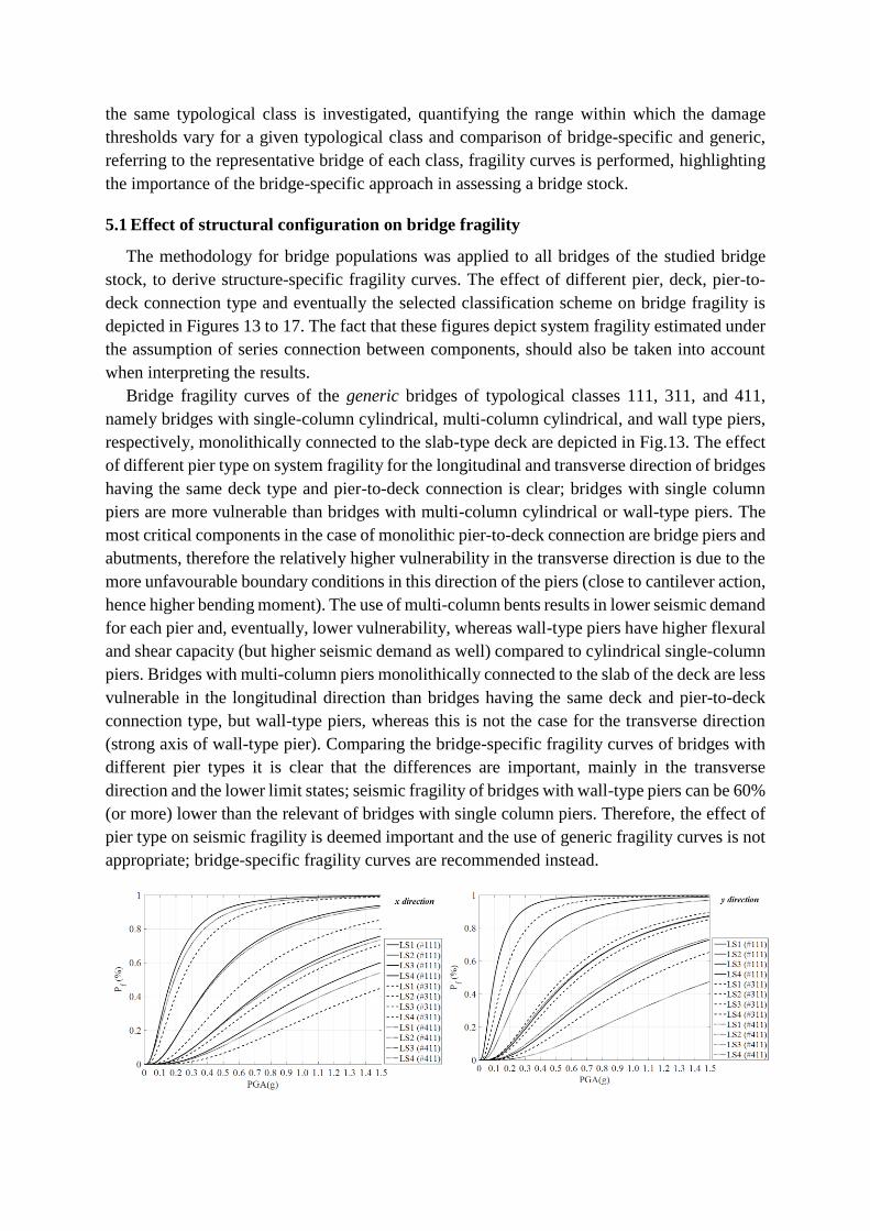
Bridge fragility curves of the generic bridges of typological classes 111, 311, and 411,
namely bridges with single-column cylindrical, multi-column cylindrical, and wall type piers,
respectively, monolithically connected to the slab-type deck are depicted in Fig.13. The effect
of different pier type on system fragility for the longitudinal and transverse direction of bridges
having the same deck type and pier-to-deck connection is clear; bridges with single column
piers are more vulnerable than bridges with multi-column cylindrical or wall-type piers. The
most critical components in the case of monolithic pier-to-deck connection are bridge piers and
abutments, therefore the relatively higher vulnerability in the transverse direction is due to the
more unfavourable boundary conditions in this direction of the piers (close to cantilever action,
hence higher bending moment). The use of multi-column bents results in lower seismic demand
for each pier and, eventually, lower vulnerability, whereas wall-type piers have higher flexural
and shear capacity (but higher seismic demand as well) compared to cylindrical single-column
piers. Bridges with multi-column piers monolithically connected to the slab of the deck are less
vulnerable in the longitudinal direction than bridges having the same deck and pier-to-deck
connection type, but wall-type piers, whereas this is not the case for the transverse direction
(strong axis of wall-type pier). Comparing the bridge-specific fragility curves of bridges with
different pier types it is clear that the differences are important, mainly in the transverse
direction and the lower limit states; seismic fragility of bridges with wall-type piers can be 60%
(or more) lower than the relevant of bridges with single column piers. Therefore, the effect of
pier type on seismic fragility is deemed important and the use of generic fragility curves is not
appropriate; bridge-specific fragility curves are recommended instead.
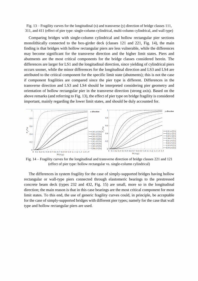
Fig. 13 – Fragility curves for the longitudinal (x) and transverse (y) direction of bridge classes 111,
311, and 411 (effect of pier type: single-column cylindrical, multi-column cylindrical, and wall type)
Comparing bridges with single-column cylindrical and hollow rectangular pier sections
monolithically connected to the box-girder deck (classes 121 and 221, Fig. 14), the main
finding is that bridges with hollow rectangular piers are less vulnerable, while the differences
may become significant for the transverse direction and the higher limit states. Piers and
abutments are the most critical components for the bridge classes considered herein. The
differences are larger for LS1 and the longitudinal direction, since yielding of cylindrical piers
occurs sooner, while the minor differences for the longitudinal direction and LS3 and LS4 are
attributed to the critical component for the specific limit state (abutments); this is not the case
if component fragilities are compared since the pier type is different. Differences in the
transverse direction and LS3 and LS4 should be interpreted considering pier geometry and
orientation of hollow rectangular pier in the transverse direction (strong axis). Based on the
above remarks (and referring to Fig. 13), the effect of pier type on bridge fragility is considered
important, mainly regarding the lower limit states, and should be duly accounted for.
Fig. 14 – Fragility curves for the longitudinal and transverse direction of bridge classes 221 and 121
(effect of pier type: hollow rectangular vs. single-column cylindrical)
The differences in system fragility for the case of simply-supported bridges having hollow
rectangular or wall-type piers connected through elastomeric bearings to the prestressed
concrete beam deck (types 232 and 432, Fig. 15) are small, more so in the longitudinal
direction; the main reason is that in this case bearings are the most critical component for most
limit states. To this end, the use of generic fragility curves could, in principle, be acceptable
for the case of simply-supported bridges with different pier types; namely for the case that wall
type and hollow rectangular piers are used.

Fig. 15 – Fragility curves for the longitudinal and transverse direction of bridge classes 432 and 232
(effect of pier type: hollow rectangular vs. wall-type)
The effect of different deck type namely slab or box girder, on the fragility of bridges having
single-column cylindrical piers connected to deck through elastomeric bearings (classes 122
and 112), is in general minor, as shown in Fig. 16. It should be noted, though, that the effect is
larger for the longitudinal direction. The use of generic fragility curves for the case of simply-
supported bridges with different deck type is, in general, acceptable, mainly for the transverse
direction.
Fig. 16 – Fragility curves for the longitudinal and transverse direction of bridge classes type 112, type
122 (effect of deck type: slab or box girder)
Finally, the effect of pier-to-deck connection (monolithic or through elastomeric bearings)
on bridges having single-column cylindrical piers and slab-type deck, is depicted in Fig. 17
(types 112 and 111). It is seen that fragility of monolithic bridges is lower for all limit states
and in both directions. The latter is due to the fact that different components, namely bearings
and piers, are critical for the seismic performance of each bridge class, mainly in the
longitudinal direction.

Fig. 17 – Fragility curves for the longitudinal and transverse direction of bridge classes 112 and 111
(effect of pier-to-deck connection: monolithic vs. through bearings).
From the comparison of bridge-specific fragility curves derived for the generic bridge in
each typological class, it is concluded that bridge fragility varies among different classes, which
establishes the importance of the classification scheme adopted. Among the features considered
in defining the typological classes, the pier type and pier-to-deck connection type were found
to affect bridge fragility the most, compared to the deck type (which is the most critical bridge
component when non-seismic loads are considered). The maximum differentiation in fragility
curves of different bridge classes was found in the case of monolithic pier-to-deck connection
and varying pier types, because in that case piers are the most vulnerable component and their
type (single-column cylindrical, multi-column cylindrical, hollow rectangular, wall, etc.)
strongly affects the dynamic characteristics of the bridge and, hence, its seismic performance.
5.2 Effect of geometric properties on bridge fragility
The effect of pier height(s) and total bridge length on bridge fragility is evaluated comparing
the bridge-specific limit state thresholds (mean PGA values) for all bridges and each bridge
class of the inventory (Figures 20 to 22). The variation of threshold values is clear, highlighting
the effect of bridge geometry (pier height and total length) on seismic fragility and the
importance of bridge-specific fragility curves in the seismic assessment of a bridge stock. In
Fig. 20, the variation of limit state threshold values in PGA terms with varying maximum pier
height is presented. Since the range of pier heights and the number of piers are not accounted
for, an equivalent height (Hequiv) is proposed (Eq. (3) and Fig. 21), considering the heights of
all piers (hi) and the number of piers (n), in order to evaluate the effect of pier height on system
fragility; clearly this is a simplified way to address the issue, not appropriate for extreme cases,
such as the presence of a short pier in the middle of the bridge (found in some poorly designed
existing bridges).
3
n 1
3i
1
eqhi
nh
(3)
As seen in Fig. 21, bridges having shorter piers (lower heq) are in general more vulnerable,
however it should be highlighted that the threshold values refer to the bridge system rather than
the individual components. The general trend and the relevant limit state threshold variation is
depicted in Fig. 21 for different bridge classes and limit states (piers are the most critical
components for the cases shown).

Fig. 20 – Effect of maximum pier height on seismic fragility of different bridge classes (mean PGA values for
LS4)
Fig. 21– Effect of equivalent pier height on seismic fragility of different bridge classes
Finally, based on Fig. 22, it appears that the effect of total length on bridge system fragility
varies, depending on the bridge class and structural system; no clear trends can be identified in
this case, as several other factors affect the calculated PGA thresholds.
Fig. 22 – Effect of total bridge length on seismic fragility of different bridge classes
Summarising, the effect of geometric properties on bridge fragility is found to be significant,
as the limit state thresholds for bridges classified within the same class may differ by up to
60%; hence, the necessity for bridge-specific fragility analysis clearly emerges.
5.3 Differentiation of seismic fragility within the same typological class
As already mentioned, most of the available methodologies in the literature propose the use
of generic fragility curves for all bridges that fall within the same category, under the

assumption that the seismic performance of all bridges in the category is similar. The
limitations of this assumption are investigated here, by considering the bridge-specific fragility
curves for all bridges within the two most common classes of the studied road network (types
232 and 221, Fig. 12).
Table 10. Limit state thresholds in PGA terms for all bridges of typological class 232 (both directions)
232
Fragility (Direction x) Fragility (Direction y)
LS1 LS2 LS3 LS4 LS1 LS2 LS3 LS4 Lspan (m) Hpier (m) Ltot (m) Hmax
(m)
1 (repr.) 0.12 0.36 0.75 1.01 0.15 0.37 0.65 1.26 40 21.0÷50.60 280 50.6
2 0.13 0.37 0.75 1.50 0.13 0.38 0.74 1.68 36.3÷37.50 9.4÷26.92 335.1 26.92
3 0.11 0.28 0.53 0.90 0.11 0.23 0.65 1.45 36 11.4÷41.01 216 41.01
4 0.12 0.32 0.80 0.93 0.16 0.32 0.70 0.94 40 12.94÷38.24 200 38.24
5 0.14 0.28 0.79 1.51 0.20 0.45 0.95 1.61 36.95÷38.0
5 16.3÷30.27 150 30.27
6 0.15 0.40 0.89 1.44 0.22 0.45 0.89 1.78 39.1÷39.50 12.75÷30.98 157.2 30.98
7 0.15 0.45 0.89 1.41 0.18 0.38 0.75 1.45 40 12.75÷30.98 200 30.98
8 0.13 0.30 0.75 1.33 0.12 0.28 0.55 1.49 39.1÷39.50 12.75÷30.98 157.2 30.98
mean 0.13 0.35 0.77 1.25 0.16 0.36 0.74 1.46
211.94 35.00
standar
d
deviatio
n
0.015 0.061 0.113 0.262 0.039 0.077 0.131 0.263 65.39 7.80
COV 11.11% 17.67% 14.66% 20.90
% 24.61% 21.65% 17.84% 18.06% 30.85%
22.29
%
Table 11. Limit state thresholds in PGA terms for all bridges of typological class 221 (both directions)
221
Fragility (Direction x) Fragility (Direction y)
LS1 LS2 LS3 LS4 LS1 LS2 LS3 LS4 Lspan (m) Hpier (m) Ltot (m) Hmax
(m)
1 (repr.) 0.35 0.68 0.86 1.33 0.30 0.75 1.19 2.02 61.5÷112.1 41.30÷45.23 234.1 45.23
2 0.30 0.76 0.83 1.07 0.48 0.70 1.21 2.38 94.5÷160 55.00÷58.00 349 58
3 0.36 0.93 1.23 1.74 0.54 0.77 1.36 2.58 80÷120 34.20÷36.41 290 36.41
4 0.16 0.59 0.98 1.81 0.24 0.55 0.97 1.39 75.6÷120 28.12÷63.39 636.2 63.39
5 0.33 0.79 1.12 1.33 0.41 0.77 1.36 2.58 60.75÷101.5 34÷63.03 426 63.03
6 0.24 0.89 1.13 1.39 0.45 0.70 1.17 2.40 91÷144 39÷45.10 326 45.10
7 0.36 0.72 0.95 1.35 0.35 0.77 1.34 2.32 61÷107 29.12÷87.83 457 87.83
8 0.37 0.76 0.96 1.50 0.30 0.62 1.09 2.30 64.3÷118.6 35.86÷44.89 247.2 44.89
9 0.36 0.72 0.95 1.35 0.47 0.72 0.95 2.50 85 32.47 170 32.47
10 0.29 0.75 1.04 1.80 0.43 0.62 1.09 2.32 80÷86 46.08 166 46.08
11 0.41 0.65 0.82 1.42 0.42 0.75 1.29 2.05 75÷80 38.37 155 38.37
mean 0.32 0.75 0.99 1.46 0.40 0.70 1.18 2.26
314.23 50.98
standard
deviation 0.070 0.098 0.131 0.231 0.091 0.074 0.147 0.341 147.49 15.97
COV 21.97% 13.09% 13.28% 15.81% 22.81% 10.60% 12.44% 15.11% 46.94% 31.32%
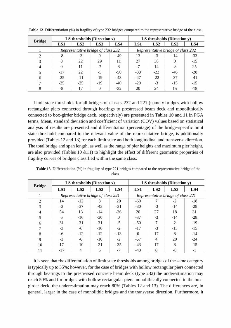
Table 12. Differentiation (%) in fragility of type 232 bridges compared to the representative bridge of the class.
Bridge LS thresholds (Direction x) LS thresholds (Direction y)
LS1 LS2 LS3 LS4 LS1 LS2 LS3 LS4
1 Representative bridge of class 232 Representative bridge of class 232
2 -8 -3 0 -49 13 -3 -14 -33
3 8 22 29 11 27 38 0 -15
4 0 11 -7 8 -7 14 -8 25
5 -17 22 -5 -50 -33 -22 -46 -28
6 -25 -11 -19 -43 -47 -22 -37 -41
7 -25 -25 -19 -40 -20 -3 -15 -15
8 -8 17 0 -32 20 24 15 -18
Limit state thresholds for all bridges of classes 232 and 221 (namely bridges with hollow
rectangular piers connected through bearings to prestressed beam deck and monolithically
connected to box-girder bridge deck, respectively) are presented in Tables 10 and 11 in PGA
terms. Mean, standard deviation and coefficient of variation (COV) values based on statistical
analysis of results are presented and differentiation (percentage) of the bridge-specific limit
state threshold compared to the relevant value of the representative bridge, is additionally
provided (Tables 12 and 13) for each limit state and both longitudinal and transverse direction.
The total bridge and span length, as well as the range of pier heights and maximum pier height,
are also provided (Tables 10 &11) to highlight the effect of different geometric properties of
fragility curves of bridges classified within the same class.
Table 13. Differentiation (%) in fragility of type 221 bridges compared to the representative bridge of the
class.
Bridge LS thresholds (Direction x) LS thresholds (Direction y)
LS1 LS2 LS3 LS4 LS1 LS2 LS3 LS4
1 Representative bridge of class 221 Representative bridge of class 221
2 14 -12 3 20 -60 7 -2 -18
3 -3 -37 -43 -31 -80 -3 -14 -28
4 54 13 -14 -36 20 27 18 31
5 6 -16 -30 0 -37 -3 -14 -28
6 31 -31 -31 -5 -50 7 2 -19
7 -3 -6 -10 -2 -17 -3 -13 -15
8 -6 -12 -12 -13 0 17 8 -14
9 -3 -6 -10 -2 -57 4 20 -24
10 17 -10 -21 -35 -43 17 8 -15
11 -17 4 5 -7 -40 0 -8 -1
It is seen that the differentiation of limit state thresholds among bridges of the same category
is typically up to 35%; however, for the case of bridges with hollow rectangular piers connected
through bearings to the prestressed concrete beam deck (type 232) the underestimation may
reach 50% and for bridges with hollow rectangular piers monolithically connected to the box-
girder deck, the underestimation may reach 80% (Tables 12 and 13). The differences are, in
general, larger in the case of monolithic bridges and the transverse direction. Furthermore, it

should be outlined that differentiation in limit state thresholds (mean value), compared to that
of the representative bridge of the class, is lower when the geometric properties (pier height,
bridge length, etc.) are similar.
5.3.1. Comparison of bridge-specific and generic fragility curves
Bridge-specific fragility curves for all bridges in class 232 (hollow rectangular piers
connected through bearings to the prestressed concrete beam deck) and 221 (piers
monolithically connected to the box-girder bridge deck) were derived and compared to the
fragility curves of the generic bridge, representative of each class. The results are depicted in
Figures 23 and 24, along with upper and lower threshold values (dashed lines - range of
thresholds) for each limit state.
Fig. 23 – Fragility of the generic bridge in class type 232 and range of damage thresholds
Fig. 24 – Fragility of the generic bridge in class type 221 and range of damage thresholds
As far as bridge class 232 is concerned, the variation of upper and lower level fragilities
compared to that of the generic bridge is small, therefore fragility curves of the bridge selected
as representative can be used for all bridges that fall within the same category for the
longitudinal direction and LS1 to LS3. The range of threshold values is fairly narrow in the
longitudinal direction (25% variation from the generic bridge) for lower limit states, however
it broadens for higher earthquake intensity and limit states and for the transverse direction,
being dependent both on the component that is critical for each limit state and the direction.
The variation of upper and lower level fragilities for bridge class type 221 is smaller for LS2
to LS4 but larger for LS1. In general, the use of the fragility curves of the generic bridge for

all those in the same category may underestimate or overestimate fragility by up to 35%,
however in some cases (i.e. LS1 for bridge class 221 and LS4 for class 221) the underestimation
is up to 50%.
6 CONCLUSIONS
The relevance of bridge-specific fragility analysis was assessed herein. First, the effect of
varying component and system properties on both capacity and (seismic) demand was
quantified. Then the effect of structural system and key geometric properties on bridge fragility
was assessed. The foregoing allowed to subsequently check the limitations of the assumption
that generic fragility curves can be used for bridges classified within the same category,
referring to a realistic bridge stock. Both structural system (pier type, deck type and pier-to-
deck connection) and geometric properties were found to substantially affect bridge fragility.
The use of generic fragility curves may become acceptable under certain circumstances,
namely for bridges with the same pier type and pier-to-deck connection having a different deck
type, and bridges with the same deck type and pier-to-deck connection when pier type is either
wall-type or hollow rectangular (i.e. very stiff cross section). However, this is only true when
bridge geometries, namely pier heights and bridge length, are similar, since the effect of
geometric properties on bridge fragility was found to be significant (up to 60%). Moreover, the
use of generic fragility curves for bridges belonging to the same class were found to
overestimate (up to 35%) or underestimate (up to 50%) bridge fragility, depending on the limit
state and critical direction considered. The use of generic fragility curves seems more
consistent for simply-supported bridges and the limit states 2 and 3.
Summarising, the most important findings are listed below:
Limit state thresholds (bridge capacity) are highly affected by component properties and the
demand parameter selected as a proxy for damage; hence, use of component-specific values
is relevant and often necessary.
Uncertainty in seismic demand generally increases with earthquake intensity, being affected
by the inelastic behaviour of the component studied, the record-to-record variability, and
the criteria for earthquake motion selection; uncertainty level varies among critical
components (piers-abutments-bearings) and bridge directions.
The total uncertainty of bridge system (βtot), calculated in bridge-specific fragility analysis,
was found to vary from 0.72 to 0.82, which are higher than 0.6, the value commonly used
in the literature; it should be noted that these values also include uncertainty due to record-
to-record variability.
Pier type has an important effect on system fragility for the case of bridges with box-girder
decks and monolithic pier-to-deck connection, as piers are the most critical component for
this bridge type. The effect of pier type on the fragility of simply-supported (through
elastomeric bearings) bridges is lower, as the bearings are the most critical component for
this bridge class for most limit states.
Bridges with single-column cylindrical piers monolithically connected to slab or box-girder
decks are more vulnerable than similar bridges having multi-column cylindrical, wall-type,
or hollow rectangular piers. Among bridges with monolithic pier-to-deck connection, those

with hollow rectangular piers monolithically connected to box-girder deck are the less
vulnerable class (transverse direction).
The effect of deck type on fragility of bridges having single-column cylindrical piers
connected to the deck through elastomeric bearings is in general minor.
Regarding the effect of pier-to-deck connection, monolithic bridges are less vulnerable for
all limit states and both bridge directions compared to simply-supported bridges; different
components are critical in each case (piers and bearings, respectively).
The variation of limit state thresholds within a bridges class, due to different pier heights
and total length, highlights the need for bridge-specific fragility curve development, as limit
state thresholds for bridges with varying geometric properties (belonging to the same class)
may vary by up to 60%.
The use of generic bridge fragility curves for all bridges in a typological class may
underestimate or overestimate fragility, typically by up to 35%; however in some cases the
underestimation may reach 50% (or even more), which is clearly an issue of concern and a
good reason for using bridge-specific curves.
For simply-supported bridges (prestressed concrete beam deck, bearing-supported to the
piers), the range of LS threshold values is generally fairly narrow for the longitudinal
direction and the lower limit states (LS2 & LS3), but it increases for higher earthquake
intensity and higher limit states (heavy damage, failure). For the transverse direction, the
variation is higher for the lower limit states as well.
For the studied case of monolithic bridges (hollow rectangular piers monolithically
connected to the box-girder of the deck), the range of limit state thresholds is broader, mainly
for the lower limit states and the transverse direction, as the seismic performance of
monolithic bridges is highly dependent on varying properties and boundary conditions of
the piers, which strongly affect the dynamic characteristics of the bridge. However, the range
is narrower for higher limit states (LS3 & LS4), compared to simply-supported bridges.
Based on the above, the need for bridge-specific fragility analysis emerges since, the use of
generic fragility curves can, in several cases, significantly affect the reliability of a road
network assessment. Therefore, the concept of bridge-specific fragility analysis, recently
proposed in literature, seems to be a step in the right direction.
ACKNOWLEDGEMENTS
This research has been co-financed by the European Union (European Social Fund – ESF) and
Greek national funds through the Operational Programme “Education and Lifelong Learning”
of the National Strategic Reference Framework (NSRF) – Research Funding Program:
ARISTEIA II: Reinforcement of the interdisciplinary and/or interinstitutional research and
innovation. The authors would like to thank Egnatia Odos S.A. for providing the data for the
case study bridges, and all participants to the RETIS-Risk research programme for their
cooperation in this multi-disciplinary project.
7 REFERENCES
Avşar, Ö., Yakut, A., & Caner, A. (2011). Analytical Fragility Curves for Ordinary Highway
Bridges in Turkey. Earthquake Spectra, 27(4), 971–996.
Banerjee, S., & Shinozuka, M. (2007). Nonlinear Static Procedure for Seismic Vulnerability
Assessment of Bridges. Computer-Aided Civil and Infrastructure Engineering, 22(4),
293–305.
Basoz, N., Kiremidjian, A., King, S., & Law, K. (1999). Statistical Analysis of Bridge Damage
Data from the 1994 Northridge, CA, Earthquake. Earthquake Spectra, 15(1), 25–54.
Berry, M., & Eberhard, M. (2003). Performance Models for Flexural Damage in Reinforced
Concrete Columns. University of Washington.
Biskinis, D. E., & Fardis, M. N. (2010). Deformations at flexural yielding of members with
continious or lap-spliced bars. Structural Concrete, 11(2), 127–138.
Biskinis, D., & Fardis, M. N. (2010). Flexure-controlled ultimate deformations of members
with continious or lap-spliced bars. Structural Concrete, 11, 93–108.
Boussias, E., Palios, X., Alexakis, C., Strepelias, E., Fardis, M., & Raptopoulos, S. (2008).
Experimental and analytical study of seismically isolated bridges with or without
additional damping. In 3rd Hellenic Conference of Earhquake Engineering and
Engineering Seismology. 5-7 November, Athens, Greece (in Greek).
Caltrans Structures Seismic Design Criteria. (2010). Sacramento, California.
Cardone, D. (2013). Displacement limits and performance displacement profiles in support of
direct displacement-based seismic assessment of bridges. Earthquake Engineering &
Structural Dynamics, 43(8), 1239–1263.
Cardone, D., Perrone, G., & Sofia, S. (2011). A performance-based adaptive methodology for
the seismic evaluation of multi-span simply supported deck bridges. Bulletin of
Earthquake Engineering , 9(5), 1463-1498.
Cardone, D., Perrone, G., & Dolce, M. (2007). Seismic risk assessment of highway bridges. In
1st US-Italy Seismic Bridge Workshop. Pavia, Italy.
Choi, E. (2004). Seismic fragility of typical bridges in moderate seismic zones. Engineering
Structures, 26(2), 187–199.
Choi, E., DesRoches, R., & Nielson, B. (2004). Seismic fragility of typical bridges in moderate
seismic zones. Engineering Structures, 26(2), 187–199.
Crowley, H., Colombi, M., Silva, V., Monteiro, R., Ozcebe, S., Fardis, M., … Askouni, P.
(2011). SYNER-G : Systemic Seismic Vulnerability and Risk Analysis for Buildings,
Lifeline Networks and Infrastructures Safety Gain. University of Pavia, Italy.
De Felice, G., & Giannini, R. (2010). An Efficient Approach for Seismic Fragility Assessment
with Application to Old Reinforced Concrete Bridges. Journal of Earthquake
Engineering, 14(2), 231–251.
DesRoches, R., Padgett, J., Ramanathan, K., & Dukes, J. (2012). Feasibility Studies for
Improving Caltrans Bridge Fragility Relationships. Rep. CA12-1775, Georgia Institute
of Technology, Atlanta, U.S.A.
Dukes, J. D. (2013). Application of Bridge Specific Fragility Analysis in the Seismic Design
Process of Bridges in California. PhD Thesis, Georgia Institute of Technology, Georgia.
Dutta, A. (1999). On Energy Based Seismic Analysis and Design of Highway Bridges. State
University of New York, Buffalo.
Dutta, A., & Mander, J. B. (1998). Seismic fragility analysis of highway bridges. In INCEDE-
MCEER Center-to-Center Workshop on Earthquake Engineering Frontiers in
Transportation Systems. Tokyo, Japan.
Elnashai, A. S., Borzi, B., & Vlachos, S. (2004). Deformation-based vulnerability functions for

RC bridges. Structural Engineering and Mechanics, 17(2), 215–244.
Erduran, E., & Yakut, A. (2004). Drift based damage functions for reinforced concrete
columns. Computers & Structures, 82, 121–130.
FHWA. (2006). Seismic Retrofitting Manual for Highway Structures: Part1-Bridges. FHWA-
HRT-06-032.
Ghosh, J., Padgett, J. E., & Dueñas-Osorio, L. (2013). Surrogate modeling and failure surface
visualization for efficient seismic vulnerability assessment of highway bridges.
Probabilistic Engineering Mechanics, 34, 189–199.
HAZUS: Earthquake loss estimation methodology, 2015. Technical Manual, National Institute
of Building for the Federal Emergency Managment Agency, Whashington, D.C.
Hwang, H., Liu, J. B., & Chiu, Y.-H. (2001). Seismic Fragility Analysis of Highway Bridges.
The University of Memphis.
Kappos, A. J. (1991). Analytical Prediction of the Collapse earthquake for R/C buildings :
Suggested Methodology. Earthquake Engineering & Structural Dynamics, 20, 167–176.
Karim, K. R., & Yamazaki, F. (2001). Effect of earthquake ground motions on fragility curves
of highway bridge piers based on numerical simulation. Earthquake Engineering &
Structural Dynamics, 30(12), 1839–1856.
Karim, K. R., & Yamazaki, F. (2003). A simplified method of constructing fragility curves for
highway bridges. Earthquake Engineering & Structural Dynamics, 32(10), 1603–1626.
Konstantinidis, D., Kelly, J. M., & Makris, N. (2008). Experimental investigations on the
seismic response of bridge bearing. Berkeley.
Lee, J.-H., Choi, J.-H., Hwang, D.-K., & Kwahk, I.-J. (2014). Seismic performance of circular
hollow RC Bridge columns. KSCE Journal of Civil Engineering, 1–12.
Lu, Y., Gu, X., & Guan, J. (2005). Probabilistic Drift Limits and Performance Evaluation of
Reinforced Concrete Columns. Journal of Structural Engineering, ASCE, 131(6), 966–
978.
Mackie, K. R., & Stojadinovic, B. (2007). R-Factor Parameterized Bridge Damage Fragility
Curves. Journal of Bridge Engineering, 12(4), 500–510.
Mackie, K., & Stojadinovic, B. (2004). Fragility Curves For Reinforced Concrete Highway
Overpass Bridges. In 13th World Conference on Earthquake Engineering. Vancouver,
B.C., Canada.
Mander, J. B., Priestley, M. J. N., & Park, R. (1988). Theoretical Stress-Strain Model for
Confined Concrete. Journal Of Structural Engineering, 114(8), 1804–1826.
Mander, J., & Basöz, N. (1999). Enhanchement of the Highway Transportation Lifeline Module
in HAZUS. Final Pre-Publication Draft (type 7) prepared for National Institute of Building
Sciences (NIBS).
McKeena, F., & Fenves, G. L. (2015). Open System for Earthquake Engineering Simulation.
Pacific Earthquake Engineering Research Center.
Moschonas, I. F., Kappos, A. J., Panetsos, P., Papadopoulos, V., Makarios, T., & Thanopoulos,
P. (2009). Seismic fragility curves for greek bridges: methodology and case studies.
Bulletin of Earthquake Engineering, 7(2), 439–468.
Nielson, B. G. (2005). Analytical Fragility Curves for Highway Bridges in Moderate Seismic
Zones Analytical Fragility Curves for Highway Bridges in Moderate Seismic Zones.
PhD Thesis, Georgia Institute of Technology, Atlanta.
Nielson, B. G., & DesRoches, R. (2007a). Analytical Seismic Fragility Curves for Typical
Bridges in the Central and Southeastern United States. Earthquake Spectra, 23(3), 615.
Nielson, B. G., & DesRoches, R. (2007b). Seismic fragility methodology for highway bridges
using a component level approach. Earthquake Engineering and Structural Dynamics, 36,
823–839.
Papanikolaou, V. K. (2012). Analysis of arbitrary composite sections in biaxial bending and

axial load. Computers and Structures, 98-99, 33–54.
Priestley, M. J. N., & Ranzo, G. (2000). Seismic performance of large rc circular hollow
columns. In 12th World Conference of Earthquake Engineering (pp. 1–8). Auckland, New
Zealand.
Priestley, M. J. N., Seible, F., & Calvi, G. M. (1996). Seismic Design and Retrofit of Bridges.
In J. Willey . New York.
Ramanathan, K. N. (2012). Next Generation Seismic Fragility Curves for California Bridges
Incorporating the Evolution in Seismic Design Philosophy. PhD Thesis, Georgia Institute
of Technology, Georgia.
Shinozuka, M., Feng, M. Q., Kim, H., & Kim, S.-H. (2000). Nonlinear Static Procedure for
Fragility Curve Development. Journal of Engineering Mechanics, ASCE, 126(12), 1287–
1295.
Shinozuka, M., Feng, M. Q., Lee, J., & Naganuma, T. (2000). Statistical Analysis of fragility
curves. Journal of Engineering Mechanics, ASCE, 126(12), 1224–1231.
Stefanidou, S. P. (2017). Software for Bridge-Specific Fragility Analysis. MOJ Civil
Engineering, 3(5), 1–7.
Stefanidou, S.P. & Kappos, A. J. (2015). Methodology for the development of structure-
specific fragility curves for bridges in a roadway network. Proceed. COMPDYN 2015,
Crete, vol. I, 1780-1798.
Stefanidou, S. P. & Kappos, A. J. (2017). Methodology for the development of bridge-specific
fragility curves. Earthquake Engineering & Structural Dynamics, 46, 73–93.
Tavares, D. H., Padgett, J. E., & Paultre, P. (2012). Fragility curves of typical as-built highway
bridges in eastern Canada. Engineering Structures, 40, 107–118.
Tsionis, G., & Fardis, M. N. (2012). Seismic Fragility of Concrete Bridges with Deck
Monolithically Connected to the Piers or Supported on Elastomeric Bearings. In 15th
World Conference of Earthquake Engineering. Lisbon, Portugal.
Yi, J., Kim, S., & Kushiyama, S. (2007). PDF interpolation technique for seismic fragility
analysis of bridges. Engineering Structures, 29(7), 1312–1322.
Zhang, J., Huo, Y., Brandenberg, S. J., & Kashighandi, P. (2008). Effects of structural
characterizations on fragility functions of bridges subject to seismic shaking and lateral
spreading. Earthquake Engineering and Engineering Vibration, 7(4), 369–382.
Zhong, J., Gardoni, P., & Rosowsky, D. (2012). Closed-form seismic fragility estimates,
sensitivity analysis and importance measures for reinforced concrete columns in two-
column bents. Structure and Infrastructure Engineering, 8(7), 669–685.
ANNEX A – β values for all pier types (global demand parameter, see table 4)
Hollow Cylindrical Piers
0
1
2 3
4
5 R2
1H -5.996 -0.445 -0.007 -0.198 -0.470 -0.117 0.74
2H -5.285 -0.385 +0.224 -0.352 +0.106 -0.0013 0.82
3H -3.867 -0.287 -0.084 -0.486 -0.433 +0.375 0.82
4H -5.863 -0.308 -0.119 -0.885 -0.219 +0.031 0.80
Rectangular Piers (Strong direction h)
0
1
2 3
4
5 R2
1H -5.695 -0.595 +0.014 -0.076 -0.549 +0.080 0.61

2H -5.520 -0.736 +1.315 -0.200 -0.120 +0.018 0.85
3H -0.643 -0.673 +1.165 -0.210 -0.262 +0.975 0.62
4H -2.861 -0.611 +0.426 -0.146 -0.114 +0.249 0.79
Rectangular Piers (Weak direction b) R2
0
1
2 3
4
5
1H -5.290 -0.386 +1.350 -0.106 -0.526 +0.101 0.74
2H -5.350 -0.718 +1.073 -0.085 -0.089 +0.021 0.75
3H -1.531 -0.639 +0.867 -0.284 -0.109 +0.772 0.67
4H -2.518 -0.630 +0.845 -0.252 -0.106 +0.386 0.60
Hollow Rectangular Piers (Strong direction h) R2
0
1
2 3
4
5
1H -7.606 +0.912 +0.957 -0.175 -0.203 -0.502 0.63
2H -5.952 +0.809 +0.857 -0.076 -0.020 -0.133 0.60
3H -4.483 +0.774 +0.459 +0.313 -0.094 -0.028 0.66
4H -4.415 +0.796 +0.264 -0.091 -0.004 -0.083 0.68
Hollow Rectangular Piers (Weak direction b) R2
0
1
2 3
4
5
1H -5.715 +0.714 -0.629 -0.104 -0.181 -0.359 0.87
2H -5.422 +0.751 -0.364 -0.020 -0.075 -0.008 0.90
3H -3.401 +0.728 -0.648 -0.156 -0.314 +0.071 0.97
4H -1.732 +0.721 -0.285 -0.573 -0.413 -0.250 0.87
Wall Piers (Strong direction h) R2
0
1
2 3
4
5
1H -6.650 -0.447 -0.230 -0.142 -0.423 +0.067 0.86
2H -4.021 -0.804 -0.645 +0.390 -0.102 -0.018 0.94
3H +2.580 -0.793 -1.003 +0.482 -0.306 +1.096 0.64
4H -3.450 -0.842 -0.054 +0.190 +0.069 +0.082 0.70
Wall Piers (Weak direction b) R2
0
1
2 3
4
5
1H -5.957 -0.861 +0.707 -0.096 -0.690 +0.115 0.67
2H -5.681 -0.871 +0.164 -0.062 -0.266 +0.044 0.88
3H 0.096 -0.810 -0.057 -0.086 -0.339 +1.075 0.70
4H -3.91 -0.864 +0.085 +0.036 -0.079 +0.009 0.85