ciphertext-only reconstruction of lfsr-based stream ciphers
TRANSCRIPT

Universita degli studi di Roma Tre
Facolta di Scienze Matematiche Fisiche e Naturali
Ciphertext-only reconstruction
of LFSR-based stream ciphers
Author:
Stefano Guarino
Supervisor:
Prof. Marco Pedicini
Academic year 2008/2009
February 2010

ii

Contents
I Introduction and Theoretical Background 1
1 Introduction to cryptology 31.1 Cryptography . . . . . . . . . . . . . . . . . . . . . . . . . . . 3
1.1.1 Symmetric cryptography . . . . . . . . . . . . . . . . . 41.1.2 Asymmetric cryptography . . . . . . . . . . . . . . . . 5
1.2 Characterization of symmetric cryptography . . . . . . . . . . 61.2.1 Block ciphers . . . . . . . . . . . . . . . . . . . . . . . 61.2.2 Stream ciphers . . . . . . . . . . . . . . . . . . . . . . 7
2 Linear Feedback Shift Registers 112.1 Linear recurring sequences in Fq . . . . . . . . . . . . . . . . 12
2.1.1 Periodicity properties . . . . . . . . . . . . . . . . . . 132.1.2 Maximal period sequences . . . . . . . . . . . . . . . . 162.1.3 Linear complexity . . . . . . . . . . . . . . . . . . . . 22
2.2 Combining linear recurring sequences . . . . . . . . . . . . . . 322.2.1 Multivariate functions over finite fields . . . . . . . . . 332.2.2 Families of linear recurring sequences . . . . . . . . . . 43
II Attacks 47
3 Correlation attack 493.1 Introduction and statistical model . . . . . . . . . . . . . . . 503.2 The attack . . . . . . . . . . . . . . . . . . . . . . . . . . . . 513.3 The algorithm . . . . . . . . . . . . . . . . . . . . . . . . . . . 553.4 Comments . . . . . . . . . . . . . . . . . . . . . . . . . . . . . 55
4 Reconstruction of stream ciphers 594.1 Introduction . . . . . . . . . . . . . . . . . . . . . . . . . . . . 594.2 Scenario . . . . . . . . . . . . . . . . . . . . . . . . . . . . . . 604.3 The BSC Model . . . . . . . . . . . . . . . . . . . . . . . . . 614.4 Preliminary analysis . . . . . . . . . . . . . . . . . . . . . . . 634.5 Reconstruction over Fq . . . . . . . . . . . . . . . . . . . . . . 66
4.5.1 Reconstruction of the registers . . . . . . . . . . . . . 68
iii

iv CONTENTS
4.5.2 The algorithm . . . . . . . . . . . . . . . . . . . . . . 754.6 Reconstruction over F2 . . . . . . . . . . . . . . . . . . . . . . 76
4.6.1 Introductory results . . . . . . . . . . . . . . . . . . . 764.6.2 Reconstruction of the registers . . . . . . . . . . . . . 784.6.3 The algorithm . . . . . . . . . . . . . . . . . . . . . . 854.6.4 Recovery of the combining function . . . . . . . . . . . 86

Preface
In 1992, the Iranian intelligence agency arrested a salesman for Crypto AG,a Swiss company specialized in communications and information security,accusing him of spying for the United States and Germany.
The salesman, Hans Buehler, on his 25th trip to Iran on behalf of Crypto,was held in solitary confinement and interrogated, in his own words, “forfive hours a day for nine months”, until Crypto paid $1 million to win hisfreedom.
This episode was only the beginning of a big inquiry on Crypto AG,accused by many of his clients (Lybia, Iran and Iraq in particular) to col-laborate with the N.S.A., the U.S. National Security Agency.
Their intelligence departments had evidence that, probably for decades,the algorithms Crypto sold them were totally known by the N.S.A. and somehidden functionalities were added to permit an easier attack.
As a consequence, all those countries, used to buy their security systemsfrom western companies, began to build their own cipher machines, nowtotally unknown to the Occidentals.
This incredible story, that seems to come out of a 007 movie, brings usto the main focus of this thesis:
is it possible to break a cryptosystem without knowing the typeof cipher being used?
Let’s make a brief overview.
When someone wants to send a message over an unprotected channel,he has to face two different problems.
First, even in a very generic acceptation of the idea of “communicatingover a channel”, such as when we write on a hard-disk or a CD, we haveto face the eventuality that some data get distorted. The data we transmit(or write) are usually altered with a certain probability, called noise of thechannel.
An entire branch of information theory, called coding theory, developedexpressly to manage this trouble, giving birth to a large set of error cor-
v

vi CONTENTS
recting codes, able to codify the informations in order to allow the detectionand correction of potential transmission errors.
In most cases, a code consists in adding to the message a redundancy,as short as possible, calculated as a function of the message. The recipientget the message together with the redundancy, both affected by the noise,and uses the relation between them to identify the most probable originalmessage.
The codes are usually a public convention and a particular channel isassociated with a particular code, especially known to be efficient with thatchannel.
The second problem, much more ancient, is to protect the message fromvoluntary attacks, mining his confidentiality, integrity or authenticity. Thisis the reign of cryptology, the art of hiding informations.
Before a message can be sent over an unprotected channel, it has to beenciphered so that only the expected recipient can decipher it and get theoriginal message.
For handiness, the process of ciphering a message follow a particular con-vention, depending on the cryptographic protocol being used, whose securityis based on the knowledge of a secret parameter, called the key.
In 1883, in a list of his fundamental principles for military ciphers, thefamous cryptographer Auguste Kerckhoffs stated what is known as the Ker-ckhoffs’ principle:
“a cryptosystem should be secure even if everything about thesystem, except the key, is public knowledge”
It means that the secrecy of the key should alone be sufficient for agood cipher to maintain at least confidentiality under an attack, and thestrength of a cryptographical protocol shouldn’t be based on the secrecy ofthe cipher’s algorithm.
Anyway, what usually happens in practice is that a message is first en-ciphered and then coded, following a protocol shared by the sender andthe recipient. The attacker doesn’t know not only the key, but neither thespecifications of the cryptosystem and the error correcting code used.
In particular, contrary to what one could think, the continuous develop-ment of intelligence agencies and espionage, with episodes like the one wereported, is driving everybody to build their own cryptosystem, making theattacker’s work more and more difficult.
What we will do in this thesis is to consider a particular class of ciphersand put ourselves in the shoes of an attacker, to try to understand howmany informations are achievable about the cipher and the original message,with the knowledge of the only material available in quite big quantity:ciphertext.

Part I
Introduction and TheoreticalBackground
1


Chapter 1
Introduction to cryptology
The term cryptology, from greek κρυπτoς (kryptos), that means “hidden”,and λoγoς (logos), that means “study”, is the “science of the secret”. Itpools two different branches:
• cryptography, whose task is defensive, using mathematical results tobuild cryptosystems able to resist to every known attack
• cryptanalysis, whose task is offensive, trying to break or at least toweak the ciphers, looking for flaws in their algorithm
These two points of view are tightly linked, two sides of the same coin,since each of them needs the knowledge of the results of the other one.
The status of the cryptanalyst, anyway, is much more comfortable, be-cause it’s easy for him to prove he broke a cipher. The cryptographer, onthe contrary, can only prove that his cipher is resistant to a certain numberof known attacks, but the so called “provable security” is almost impossibleto obtain.
Now, let’s make a little overview on the history of cryptography.
1.1 Cryptography
Hiding informations to the enemies is a necessity as old as mankind.
The first way to protect a secret message, called steganography, consistedin hiding the message itself, for example tatooing it on the shaved head ofthe messenger and waiting for his hair to grow again.
Cryptography, contrarily, does not hide the message, but hides the in-formations contained in it, so that the enemy can’t understand the message,even if he intercepts it.
We can formalize a cryptosystem as follows:
Definition 1.1. We call cryptosystem a quintuple (P, C,K, E,D), where:
3
4 CHAPTER 1. INTRODUCTION TO CRYPTOLOGY
• P, C and K are three sets, respectively of the plaintexts, the cipher-texts, and the keys
• E and D are two classes of functions parameterized by two keysK,K ′ ∈ K, such that EK : P → C is the encryption function andDK′ : C → P is the corrisponding decryption function
The trivial way to break a system is the so-called brute force attack, theexhaustive search of the key by trying every possible element of the keyspaceK. This set has a very important role, because it must be large enough notto permit such an attempt.
In general, we call attack to the cryptosystem any strategy able to reducethe set of the possible keys and/or the cost necessary to find the right one.
Usually, given an alphabet A, we have P = C = An, so both the plaintextm and the ciphertext c are n-uples of elements of A. By definition, c =EK(m) and m = DK′(c) = DK′(EK(m)).
1.1.1 Symmetric cryptography
If the key K ′ is equal to the encryption key K, the scheme is called symmet-ric. The secret key K is shared by the sender and the recipient, and hiddento anyone else.
Symmetric cryptography is very ancient, since some of the oldest knownciphers are the jewish “atbash”, cited in the Old Testament, the spartan“scytale” and the roman “Ceasar cipher”, all examples of symmetric en-cryption.
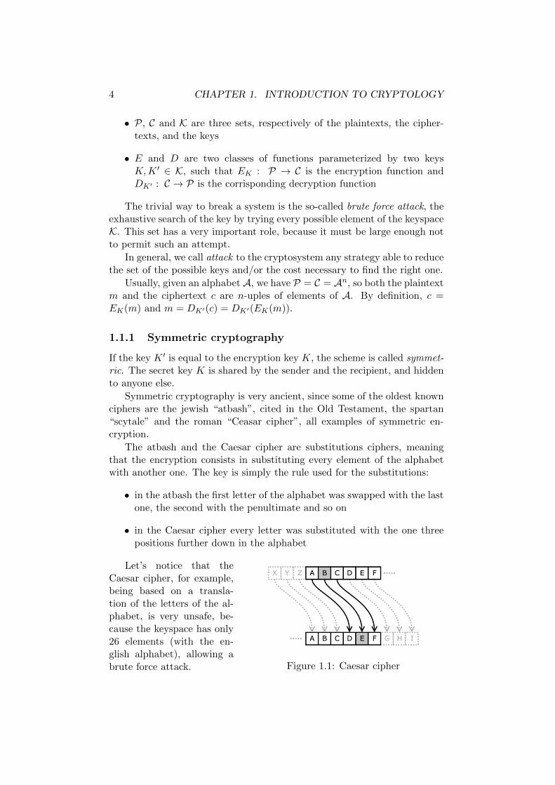
The atbash and the Caesar cipher are substitutions ciphers, meaningthat the encryption consists in substituting every element of the alphabetwith another one. The key is simply the rule used for the substitutions:
• in the atbash the first letter of the alphabet was swapped with the lastone, the second with the penultimate and so on
• in the Caesar cipher every letter was substituted with the one threepositions further down in the alphabet
Figure 1.1: Caesar cipher
Let’s notice that theCaesar cipher, for example,being based on a transla-tion of the letters of the al-phabet, is very unsafe, be-cause the keyspace has only26 elements (with the en-glish alphabet), allowing abrute force attack.

1.1. CRYPTOGRAPHY 5
Figure 1.2: A scytale
The scytale, instead, was awooden cylinder used togheterwith a leather strip. The stripwas twisted around the cilinderand the message was written inthe direction of the stick, trans-versely to the strip. The key wasthe diameter of the cylinder, be-cause twisting the strip arounda cylinder of a different thick-ness entailed the outcome of adifferent message.
We will see later in details how symmetric cryptography develloped andhow it is used nowadays.
1.1.2 Asymmetric cryptography
In the asymmetric cryptography, contrarily, every user of the cipher hashis own couple of keys, the encryption key K, called public key, and thedecryption key K ′, called private key.
The public key is public knowledge, anyone can use it to encrypt a mes-sage that only the owner of the corrispondent private key can decrypt.
Asymmetric cryptography, contrary to symmetric one, is very recent.Needing a big computational power, it was introduced only in the 70’s byW. Diffie and M. Hellman.
Asymmetric protocols are based on the so called trapdoor functions,mathematical functions, such as the discrete logarithm, easy to calculatewith the knowledge of a parameter, the trapdoor, but almost impossible tocompute without it.
Probably the most famous asymmetric cryptosystem is the RSA, thattakes his name from D. Rivest, A. Shamir and L. Adleman who developpedit in 1978. The RSA grounds on the difficulty of factorizing big integers: theprivate key is a couple of big primes (about 512 bits each) and the publickey is their product. The algorithm is shown in figure 1.3
Asymmetric cryptography, apparently easier to implement, is usuallyused only to cipher little messages, in particular to exchange a secret keylater used for a symmetric protocol.
The reasons are primarily two:
• Cost: RSA, one of the faster asymmetric protocols, is a thousandfoldslower than the DES, one of the more diffused symmetric block ciphers(see later)
• Security: the strenght of public-key cryptography is based on the com-putational complexity theory. This theory supposes the existence of

6 CHAPTER 1. INTRODUCTION TO CRYPTOLOGY
(and search for) problems impossible to solve in polynomial time, soperfect to be used in asymmetric protocols. This “non-computability”,however, hasn’t ever been proved. So what if someone finds a way, forexample, to factorize in a faster way than what is now believed possi-ble?
Figure 1.3: RSA algorithm
1.2 Characterization of symmetric cryptography
In this work we’re only interested in symmetric cryptography. It is the kindof protocols used in military and business security, mainly for the reasonsexposed above.
What follows is its basic classification in block ciphers and stream ci-phers.
1.2.1 Block ciphers
A block cipher is a symmetric key cipher operating on fixed-length groupsof digits, termed blocks, with an unvarying transformation. Usually thisciphers applies to binary transmissions, so we will refer to them in thatcontext. A formal definition follows.
Definition 1.2. Let A be an alphabet of q symbols and K be the keyspace.We call block cipher a memoryless encryption scheme which breaks up theplaintext message m ∈ A∗ into strings (called blocks) of a fixed length n,m = m1|m2| . . . |mi| . . . where each mi ∈ An, and encrypts one block at a

1.2. CHARACTERIZATION OF SYMMETRIC CRYPTOGRAPHY 7
time. The encryption transformation is EK : An → An′ , where K ∈ K isthe key used and n′ can be bigger than n.
Introduced by H. Feistel in 1973, block ciphers achieved success with theData Encryption Standard (DES), publicly released in 1976 and adopted asa U.S. government Federal Standard.
DES originally had a block size of 64 bits and a key size of 56 bits, but,as time went on, its inadequacy became apparent and a variant of DES,called Triple DES, was widely adopted as a replacement. It triple-encryptsblocks with (usually) two different keys, resulting in a 112-bit keys and 80-bitsecurity, and it is still considered secure.
DES has been superseded as a U.S. Federal Standard by the AdvancedEncryption Standard (AES), developed by two belgian cryptographers, JoanDaemen and Vincent Rijmen, and submitted under the name Rijndael. AEShas a block size of 128 bits and three possible key sizes, 128, 192 and 256bits.
In a block cipher both algorithms, EK for encryption and DK for de-cryption, accept two inputs: an input block mi of size n bits and a key K ofsize k bits, yielding an n′-bit output block. Usually n′ = n, so for each keyK, EK is a permutation (a bijective mapping) over the set of all possibleinput blocks: the key selects one permutation from the 2n! possible ones.
The block size, n, is typically 64 or 128 bits, although some ciphershave a variable block size. 64 bits was the most common length until themid-1990s, when new designs began to switch to the longer 128-bit length.One of several modes of operation is generally used along with a paddingscheme to allow plaintexts of arbitrary lengths to be formatted in n-blocksand encrypted. Each mode has different characteristics in regard to errorpropagation, ease of random access and vulnerability to certain types ofattack. Typical key sizes include 40, 56, 64, 80, 128, 192 and 256 bits, but80 bits is normally taken as the minimum key length needed to prevent bruteforce attacks.
Most block ciphers are constructed by repeatedly applying a simplerfunction, with an approach known as iterated block cipher or Feistel cipher.Each iteration is termed a round, and the repeated function is termed theround function. Typically, the number of rounds varies from 4 to 32: DEShas 16 rounds, AES has 10, 12 or 14 rounds, according to the lenght ofthe key. The round function is usually a composition of arithmetic andlogical operations (especially XOR), S-boxes (substitution boxes) and per-mutations.
1.2.2 Stream ciphers
A stream cipher is a symmetric key cipher where plaintext digits are com-bined one-to-one with a pseudorandom stream, called keystream, typically
8 CHAPTER 1. INTRODUCTION TO CRYPTOLOGY
by a modular sum (an exclusive-or (XOR) in the binary case). Formally:
Definition 1.3. LetA be an alphabet of q symbols andm = m1m2 · · ·mi · · · ∈A∗ be a message. Given a set K, let K = k1k2 · · · ki · · · ∈ K∗ be thekeystream and Eki : A → A be a family of simple substitutions on A. Astream cipher is a memoryless encryption scheme which encrypts the plain-text message m one element at a time into the ciphertext c = c1c2 · · · ci · · · ∈A∗, where ∀i ci = Eki(mi).
This class of ciphers is inspired by the so-called One-Time Pad, a streamcipher where the keystream is a random stream as long as the message, usedonly once and then changed everytime a new message has to be encrypted.
In 1949 Claude Shannon[15] showed that the OTP is unbreakable, or, inhis words, it has the property of perfect secrecy, meaning that the knowledgeof the ciphertext c gives absolutely no additional informations about theplaintext m.
In his work on Information Theory, Shannon defined a function calledentropy, that measures the uncertainty’s degree of a random variable. If Xis a random variable assuming the values x0, x1, . . . , xn each with probabilityP (X = xi) = pi, the entropy of X is defined as:
H(X) =
n∑i=0
pi log1
pi
where the base of the logarithm is the same base used to store informa-tions and the unit of measurement of the entropy, usually 2.
If we think of a message as the outcome of a random variable, Shannon’sentropy is a measure, in the sense of an expected value, of the amount ofinformation contained in a message. At the same time, it measures theaverage information content we’re missing when we do not know the valueassumed by that variable.
In terms of entropy, the perfect secrecy can then be formulated as:
H(m) = H(m|c)
where H(m) is the entropy of the plaintext m, while H(m|c) is theconditional entropy of m given the ciphertext c.
Shannon also showed that a necessary condition for perfect secrecy is
H(K) ≥ H(m)
It means that the uncertainty on the secret key must be at least as highas the one on the plaintext. If the key’s lenght is k and the elements ofthe keystream are chosen randomly and regardless one of the others, theentropy of the key is H(K) = k, so Shannon’s condition become k ≥ H(m),and this condition is obviously verified by the OTP.

1.2. CHARACTERIZATION OF SYMMETRIC CRYPTOGRAPHY 9
The OTP is, however, impossible to realize, because it implies that thesender of the message is able to communicate to the recipient a key as longas the message he wants to transmit. That’s why stream ciphers use apseudorandom key, generated from a shorter key easy to share by the parts.
Stream ciphers are a very important class of ciphers, widely used eitherin the military and governmental or in the industrial security. They arevery easy to implement both in hardware and software, much faster thanblock ciphers and, usually, have the remarkable property that an error inthe trasmission of a digit only affect that digit in the ciphertext and doesnot propagate to other parts of the message, since the plaintext digits areencrypted one at a time.
Furthermore, Shannon’s theory put strong bases for the development ofstream ciphers, since it highlights how the security of such a cipher onlydepends on the randomicity of the keystream.
We can further classificate stream ciphers into synchronous and self-synchronous ciphers.
In a synchronous stream cipher the keystream is generated independentlyfrom the ciphertext, while in a self-synchronous one a finite state machinealso uses ciphertext digits to create the keystream.
The effect of this different design is that in a self-synchronous cipher, ifciphertext digits are inserted or deleted, only a fixed number of plaintextdigits are lost in the decryption, since these ciphers have the capability ofre-establishing the synchronization.
Anyhow, in our work synchronous stream ciphers have a more preemi-nent role. We can describe them schematically as in figure 1.4.
Figure 1.4: A typical synchronous stream cipher

10 CHAPTER 1. INTRODUCTION TO CRYPTOLOGY
• the function Init generate an initial state σ0 from the key K and aninitial vector IV :
σ0 = init(K, IV )
• in every round a function f is used to update the internal state of thecipher:
σt = f(K,σt−1)
• another function g is then used to generate the keystream zt as afunction of the key and the internal state:
zt = g(K,σt)
• finally the plaintext digits mt are combined with the keystream ztthrough a function h to generate the ciphertext digits ct:
ct = h(mt, zt)
Let’s note that the function h(x, y) must be invertible in the first variable,namely there must exist a function h−1 such that ∀t mt = h−1(ct, zt).
Usually, the plaintext, keystream and ciphertext digits are elements froma finite field Fq. If h(mt, zt) := mt + zt is the modular sum, then the streamcipher is called additive. The most common case is the additive with q = 2,where the sum coincide with the bitwise XOR operation.

Chapter 2
Linear Feedback ShiftRegisters
In the description of synchronous stream ciphers we gave previously, weskipped the characterization of the keystream generator functions, probablythe most important primitive of those ciphers.
Particularly interesting in our work is a basic component of many ciphers:the Linear Feedback Shift Register (LFSR).
A shift register of length L over Fq is a register with L stages, whosestate is a sequence of L elements of Fq each one memorized in one of thestages. Governed by a clock, at every clock stroke the register undergoes atransition where every element “shift” to the next stage, but the last onewhich is outputted. The first stage, now empty, is filled with a new elementcalculated as a function of the previous state. If the input element of ashift register is a linear combination of its previous state, then the registeris called linear, shorten LFSR.
Formally, in a generic instant t the state of the register is a L-tuplest = (st, . . . , st+L−1) ∈ FLq .
The initialization of the register is s0 = (s0, . . . , sL−1) and the sequencegenerated by the LFSR is defined recursively from the initial state as
st+L =L−1∑i=0
aist+i, t ≥ 0
where ai ∈ Fq for all i and the sum obviously is modular in Fq.The stages of the register involved in the feedback function, namely those
with ai 6= 0, are termed taps.Clearly, the element st generated at time t depends only on the previous
state st−1, thus the whole sequence depends only on the initial state s0 andon the feedback coefficients ai.
In the next sections we will see more in details the properties of thesequences generated by a LFSR.
11

12 CHAPTER 2. LINEAR FEEDBACK SHIFT REGISTERS
Figure 2.1: A LFSR of length 7 over F2. The taps are in position 2 and 6,so the feedback relation is st+7 = st+2 + st+6. The present state is 0100101.
2.1 Linear recurring sequences in FqFirst of all a formal definition.
Definition 2.1. Let L be a positive integer, a Lth-order linear recurringsequence over a finite field Fq is a sequence stt∈N of elements of Fq suchthat
st+L = aL−1st+L−1 + aL−2st+L−2 + · · ·+ a0st + a ∀t ∈ N (2.1.1)
with a, ai ∈ Fq, for all i = 0, . . . , L− 1.Relation 2.1.1 is called the linear recurrence relation of the sequence, and
the terms s0, s1, . . . , sL−1, which generate the whole sequence, are called theinitial values. If a = 0 the sequence is called homogeneous, otherwise iscalled inhomogeneous.
Remark 2.1. An inhomogeneous Lth-order linear recurring sequence canalways be seen as a homogeneous (L+ 1)th-order linear recurring sequence.In fact, given relation 2.1.1 with a 6= 0, we can write
st+L = aL−1st+L−1 + · · ·+ a0st + a
st+L+1 = aL−1st+L + · · ·+ a0st+1 + a
for all t and, subtracting the two equations, we get
st+L+1 = (aL−1 + 1)st+L + (aL−2− aL−1)st+L−1 + · · ·+ (a0− a1)st+1− a0st
Now, if we put bL = aL−1 + 1, bL−i = aL−i−1 − aL−i for all i = 1, . . . , L− 1and b0 = −a0, we have the equivalent homogeneous (L + 1)th-order linearrecurring sequence
st+L+1 = bLst+L + bL−1st+L−1 + · · ·+ b1st+1 + b0st ∀t ∈ N
Hereinafter, then, we will consider only homogeneous sequences of theform
st+L = aL−1st+L−1 + aL−2st+L−2 + · · ·+ a0st ∀t ∈ N (2.1.2)

2.1. LINEAR RECURRING SEQUENCES IN FQ 13
Definition 2.2. Given a Lth-order linear recurring sequence stt∈N, wecall its tth-state vector the vector
st = (st, st+1, . . . , st+L−1) ∈ FLq
The vector s0 is called the initial state vector of the sequence.
As we have already remarked, a linear recurring sequence is completelydetermined by the initial state and the coefficients ai, so it can be seen as apair (s0,a), where a = (a0, a1, . . . , aL−1) ∈ FLq is the vector of the coefficientsof the linear recurrence relation 2.1.2.
If we consider the matrix A ∈ML(Fq) defined as
A =
0 0 · · · 0 a0
1 0 · · · 0 a1
0 1 · · · 0 a2...
.... . .
......
0 0 · · · 1 aL−1
we can write the recurrence relation as
st = st−1A = st−2A2 = · · · = s0A
t ∀t ∈ N
Note that the matrix A depends only on the linear recurrence relation2.1.2 and not on the elements of the sequence. Studying its properties,then, gives us informations on all the sequences satisfying the same relation,regardless of the initial state.
2.1.1 Periodicity properties
Recurring sequences have very interesting periodicity properties.
Definition 2.3. Let stt∈N be a sequence in Fq. If there exist two integersr > 0 and tr ≥ 0 such that
st+r = st ∀t ≥ tr
then the sequence is called ultimately periodic and r is a period of the se-quence. The smallest period r of a sequence is called its least period. Iftr = 0 then the sequence is called periodic.
Lemma 2.1. Let stt∈N be a ultimately periodic sequence whose leastperiod is r. If r is another period of the sequence, then r | r.
Proof. Let tr and t0 be to integers such that st+r = st for all t ≥ tr andst+r = st for all t ≥ t0. If r 6| r, by the euclidean division we can write

14 CHAPTER 2. LINEAR FEEDBACK SHIFT REGISTERS
r = mr + k, for some integers m ≥ 0 and 0 < k < r. Hence, for allt ≥ max(t0, tr) we have
st = st+r = st+mr+k = st+(m−1)r+k = · · · = st+k
which means that k is a period of the sequence, but that’s impossible sincek < r and r is the least period.
Definition 2.4. Let stt∈N be a ultimately periodic sequence whose leastperiod is r, then we call the preperiod t of the sequence the smallest non-negative integer such that the equality st+r = st holds for all t ≥ t.
The following Proposition states that, as we would expect, in an ulti-mately periodic sequence, the preperiod t is the same for every period of thesequence, so every periodicity begins from the same point.
Proposition 2.1. Let stt∈N be a ultimately periodic sequence whosepreperiod is t. Let r be any period of the sequence, then t is the small-est non-negative integer for which the equality st+r = st holds for all t ≥ t.
Proof. Let r be the least period of the sequence, and r any other period.We have
st+r = st ∀t ≥ tst+r = st ∀t ≥ tr
where tr is the smallest non-negative integer for which the second equalityholds.
We want to show that tr = t. From lemma 2.1 we know that r | r, sothere exists an integer h such that r = hr. Now:
• tr ≤ t: clearly it holds st = st+r = st+hr = st+r ∀t ≥ t but weknow that tr is the smallest integer for which the last equality holds,so it implies that tr ≤ t.
• tr ≥ t: by definition of t, st−1 6= st+r−1. If tr < t, then st−1 =st+r−1 = st+hr−1 = st+r−1, which contradicts the inequality above. Soit must be tr ≥ t.
Periodicity properties are particularly interesting thanks to the followingTheorem.
Theorem 2.1. For all L > 0, every Lth-order linear recurring sequence inany finite field Fq is ultimately periodic with least period r ≤ qL − 1.

2.1. LINEAR RECURRING SEQUENCES IN FQ 15
Proof. To prove the Theorem it suffices to recall that a recurring sequenceis completely determined by its initial state. Passing through the all-zerostate brings obviously to the all-zero sequence, which is ultimately periodicwith least period 1. Since any state of the sequence is a vector st ∈ FLq ,
clearly the number of possible non-zero states is qL−1, so that’s the longestpossible period.
Remark 2.2. Note that not every ultimately periodic sequence is periodic.For example, applying the recurrence relation st = st−1 to the initial state(0, 1) generates the sequence 01111 . . ., which is ultimately periodic but notperiodic, since its preperiod is the initial 0.
We can obtain periodic sequences just using the following simple result.
Proposition 2.2. Let stt∈N be a linear recurring sequence in Fq satisfyingthe recurrence relation 2.1.2. If a0 6= 0 then the sequence is periodic.
Proof. Thanks to Theorem 2.1, we know the sequence to be ultimately pe-riodic. Let r be its least period and t0 be its preperiod, so that st+r = stfor all t ≥ t0. If a0 6= 0 it is clearly invertible in Fq, thus from equation 2.1.2we have
st = a−10 (st+L − aL−1st+L−1 − · · · − a1st+1)
now, if we suppose t0 ≥ 1, we can take t = t0 − 1 and obtain
st0−1 = a−10 (st0+L−1 − aL−1st0+L−2 − · · · − a1st0)
If, otherwise, we take t = t0 − 1 + r and use the definition of periodicity wehave
st0−1+r = a−10 (st0+L−1+r − aL−1st0+L−2+r − · · · − a1st0+r)
= a−10 (st0+L−1 − aL−1st0+L−2 − · · · − a1st0)
but it means that st0−1+r = st0−1, which contradicts the definition of prepe-riod.
The previous condition is only a sufficient one, but not necessary, asshown by the following example.
Example 2.1. Every sequence (s0,a) with s0 = (g, g) (where g ∈ Fq) anda = (a0, a1) = (0, 1) is clearly periodic (st = g for all t ∈ N).
Finally, we show how the least period of a sequence is related to itsrecurrence relation.
Proposition 2.3. Let stt∈N be a Lth-order recurring sequence in Fq witha0 6= 0 and let A be its associated matrix. Thus the least period r of thesequence divides the order of A in the group GLL(Fq) of L × L invertiblematrices over Fq: r | ord(A).

16 CHAPTER 2. LINEAR FEEDBACK SHIFT REGISTERS
Proof. First of all, we have detA = (−1)L−1a0 6= 0, so actually A ∈GLL(Fq). Let m be the order of A in GLL(Fq), namely m is the lowestinteger such that Am = IL. Then
st+m = s0At+m = s0A
tAm = s0At = st
so m is a period of the sequence and by lemma 2.1 r | m.
2.1.2 Maximal period sequences
Our interest in the properties of linear recurring sequences is due to oursearch for a easy way to generate pseudo-randomic streams.
Linear recurring sequences can be easily generated by a LFSR, but usu-ally they do not have good statistical properties.
The circumstances change when the sequence has a long period, so thepurpose of this section is to recognize the features allowing to obtain arecurring sequence of longest possible period.
Definition 2.5. An impulse response sequence is a homogeneous linear re-curring sequence (d,a), such that d = (0, . . . , 0, 1).
Proposition 2.4. Let rs be the least period of a Lth-order linear recurringsequence (s0,a) and let rd be the least period of the corresponding impulseresponse sequence (d,a). Then rs | rd for all s0 ∈ FLq .
Proof. First, let dt denote the tth state vector of the impulse response se-quence. Note that dn = dm if and only if An = Am. In fact dn = dm ifand only if dn+t = dtA
n = dtAm = dm+t for all t ≥ 0, but the last relation
holds if and only if An = Am, since d,d1, . . . ,dL−1 obviously form a basisfor the L-dimensional vector space FLq over Fq.
Now, if t0 is the preperiod of (d,a), we have dt = dt+rd for all t ≥ t0. Aswe have seen, it implies that At = At+rd for all t ≥ t0, so clearly st = st+rdand then rd is a period of (s0,a). The conclusion follows from lemma 2.1.
Proposition 2.5. Let (d,a) be a Lth-order impulse response sequence inFq with a0 6= 0 and let A be its associated matrix. Then its least period ris equal to the order of A in GLL(Fq): r = ord(A).
Proof. Thanks to Proposition 2.3 we know that r | ord(A). On the otherhand, by Proposition 2.2 we know the sequence to be periodic, so dr = d.It implies, as we have seen in the proof of Proposition 2.4, Ar = A0 = IL,which implies ord(A) | r.
Associated with a linear recurring sequence are two particular polyno-mials.

2.1. LINEAR RECURRING SEQUENCES IN FQ 17
Definition 2.6. Let stt∈N be a Lth-order linear recurring sequence whoserecurrence relation is 2.1.2.
We call its characteristic polynomial the polynomial
f(X) = XL −L∑i=1
aL−iXL−i = XL − aL−1X
L−1 − · · · − a1X − a0 (2.1.3)
while its feedback polynomial is
f∗(X) = 1−L∑i=1
aL−iXi = 1− aL−1X − · · · − a0X
L (2.1.4)
Remark 2.3. Note that the feedback polynomial is the reciprocal of the char-acteristic polynomial: f∗(X) = XLf
(1X
). Hence, every property of f∗ is
restatable in terms of f and vice versa. Since the two polynomials have verydifferent shapes, the context should allow the reader to distinguish whichpolynomial we are talking about. Note, moreover, that these two polyno-mials depend only on the recurrence relation and not on the initial state.Thereafter, S(f∗) will denote the set of all sequences whose feedback polyno-mial is f∗, or analogously S(f) the set of all sequences whose characteristicpolynomial is f .
Example 2.2. Take the recurrence relation of order 2 over F5 defined byst+2 = 2st+1 + st, whose vector of coefficients is a = (1, 2).
The characteristic polynomial of the sequence is hence f(X) = X2−2X−1, while its feedback polynomial is f∗(X) = 1 − 2X −X2. Since we are inF5, they can be restated as f(X) = X2 +3X+4 and f∗(X) = 4X2 +3X+1.The relation f∗(X) = X2f
(1X
)is clearly verified.
Let’s now recall an important definition.
Definition 2.7. Let f(X) ∈ Fq[X], we call its order, denoted ord(f), thesmallest integer k such that Xk ≡ 1 mod f(X).
Remark 2.4. If stt∈N is a Lth-order linear recurring sequence over Fq whosecharacteristic polynomial is f(X) and whose associated matrix is A, f(X)is the characteristic polynomial of the matrix A: f(X) = det(A − XIL).Analogously, A is the companion matrix of f(X), so, if a0 6= 0, then A isinvertible and ord(f) = ord(A).
Thanks to the characteristic polynomial, we can recast some of the pre-vious Propositions as follows.
Theorem 2.2. Let (s0,a) be a linear recurring sequence in Fq and let f(X)be its characteristic polynomial. Then
• the least period r divides the order of f(X): r | ord(f)

18 CHAPTER 2. LINEAR FEEDBACK SHIFT REGISTERS
• the least period of the corresponding impulse sequence (d,a) equals it:r = ord(f)
Many relations between linear recurring sequences and their characteris-tic polynomials can be found on the basis of the following polynomial iden-tity. We will not prove it now, the interested reader can find the originalproof in chapter 8 of [10], while we will give an alternative proof later.
Theorem 2.3. Let stt∈N be a Lth-order homogeneous linear recurringsequence over Fq, periodic with period r. Let 2.1.2 be its recurrence relationand f(X) be its characteristic polynomial. Then the identity
f(X)s(X) = (1−Xr)h(X) (2.1.5)
holds with
s(X) = s0Xr−1 + s1X
r−2 + · · ·+ sr−2X + sr−1 ∈ Fq[X]
and
h(X) =L−1∑j=0
L−1−j∑i=0
ai+j+1siXj ∈ Fq[X]
where we set aL = −1 for convenience.
Theorems 2.2 and 2.3 lead us to the following important result.
Proposition 2.6. Let (s0,a) be a linear recurring sequence in Fq withs0 6= (0, 0, . . . , 0) and let f(X) ∈ Fq[X] be its characteristic polynomial. Iff(X) is irreducible over Fq and f(0) 6= 0, then the sequence is periodic withleast period r equal to the order of f(X): r = ord(f).
Proof. First, f(0) 6= 0 means a0 6= 0 and the periodicity of the sequencefollows from Proposition 2.2. Now, from identity 2.1.5 follows that f(X)divides (X r − 1)h(X). Since s(X) and h(X) are non-zero polynomials andsince deg(h) < deg(f), the irreducibility of f(X) implies that f(X) dividesX r− 1. It means that X r ≡ 1 mod f(X), so necessarily ord(f) | r. On theother hand r | ord(f) by Theorem 2.2, hence r = ord(f).
Let’s recap what we have seen until now.Take any Lth-order recurrence relation over a finite field Fq and let f(X)
be its characteristic polynomial. The relation defines a partition of FLq in
distinct “orbits”: for every vector v ∈ FLq , the vectors in the same orbit ofv are all the state vectors, and only those, of the sequence with v as initialvector and generated by that relation. The greatest possible least periodequals the order of f(X) and every other least period divides it. If f(X) isirreducible, then every orbit has the same size, ord(f), obviously except theorbit of the vector (0, . . . , 0) ∈ FLq , which is the only one element in its orbit.

2.1. LINEAR RECURRING SEQUENCES IN FQ 19
As we have seen, the impulse vector d = (0, . . . , 0, 1) ∈ FLq always generatesa sequence with period r = ord(f), so its orbit is always the greatest one(or one of the greatest).
Example 2.3. As in example 2.2, let’s take the recurrence relation st+2 =2st+1 + st over F5 defined by the vector a = (1, 2). The characteristicpolynomial is f(X) = X2 − 2X − 1 which is irreducible over F5. The 25elements of the set F2
5 are, then, partitioned in 3 orbits:
(0, 0) which obviously contain only the all-zero vector
(0, 1), (1, 2), (2, 0), (0, 2), (2, 4), (4, 0), (0, 4), (4, 3), (3, 0), (0, 3), (3, 1), (1, 0)
(1, 1), (1, 3), (3, 2), (2, 2), (2, 1), (1, 4), (4, 4), (4, 2), (2, 3), (3, 3), (3, 4), (4, 1)
Note that, since ord(f) = 12 and f(X) is irreducible, as we expected thenon-zero orbits both contain exactly 12 elements.
As we have already outlined, our first aim is to detect the conditionsproducing the longest possible period. Thanks to the previous results, weknow that the best we can aspire to is a recurrence relation generatingonly two orbits in FLq : the one with only the (0, . . . , 0) vector and another
one containing all the remaining qL − 1 vectors. The following result isfundamental.
Theorem 2.4. Let stt∈N be a homogeneous Lth-order linear recurringsequence whose characteristic polynomial is primitive over Fq and whoseinitial state is non-zero. Then st is periodic and its least period is r =ord(f) = qL − 1.
We call such a sequence a maximal period sequence.
Proof. The Theorem is trivial. Every primitive polynomial is irreducible, soby Proposition 2.6 r = ord(f). Moreover ord(f) = qL − 1 by definition ofprimitive polynomial.
Example 2.4. Let’s take again F25. If we choose the recurrence relation st+2 =
2st+1+2st, we have the characteristic polynomial f(X) = X2−2X−2 whichis known to be primitive over F5.
Hence, for every initial vector s0 6= (0, 0), we enter a maximal periodsequence of length r = 52−1 = 24. If we started with the impulse s0 = (0, 1),for example, the sequence would be:︷ ︸︸ ︷
0, 1, 2, 1, 1, 4, 0, 3, 1, 3, 3, 2, 0, 4, 3, 4, 4, 1, 0, 2, 4, 2, 2, 3, 0, 1, 2, . . .
The following Proposition shows that maximal period sequences alsohave the other feature we were looking for: good statistical properties.

20 CHAPTER 2. LINEAR FEEDBACK SHIFT REGISTERS
Proposition 2.7. Let S = (s0,a) be a maximal period sequence of order Lin Fq. Let m be an integer such that 1 ≤ m ≤ L and S′ any subsequence ofS of length qL +m− q. Then every non-zero sequence of length m appearsexactly qL−m− 1 times as a subsequence of S′. The distribution of patternsof fixed length m ≤ L is almost uniform.
In [18], the interested reader can find a proof of the previous Propositionand check that a sequence with such properties also satisfies the Golombsrandomness postulates.
Finally, with the following Theorem we note that, at least in some spe-cial cases, the introduction of the characteristic polynomial also permitsto explicitly represent the elements of a linear recurring sequence throughalgebraic structures over Fq.
Theorem 2.5. Let stt∈N be a Lth-order linear recurring sequence overFq whose characteristic polynomial is f(X). If the roots α1, . . . , αL of f(X)are all distinct, then for all t ≥ 0 we have
st =L∑j=1
βjαtj (2.1.6)
where β1, . . . , βL are elements of the splitting field of f(X) over Fq, uniquelydetermined by the initial state of the sequence.
Proof. First of all, given the initial state s0, . . . , sL−1 of the sequence andthe roots α1, . . . , αL of f(X), let’s take the system of linear equations
L∑j=1
αtjβj = st for all t = 0, . . . , L− 1
in the unknown β1, . . . , βL.Clearly, the matrix V associated with the system is a Vandermonde
matrix1 and it’s known that for such a matrix holds
detV =∏
1≤i<j≤L(αj − αi)
By the hypothesis on the αj , we get hence detV 6= 0, so the system admitsa solution β1, . . . , βL, whose elements are obviously in the splitting field off(X).
Now, we know that the elements of the sequence must satisfy
st+L = aL−1st+L−1 + aL−2st+L−2 + · · ·+ a0st ∀t ∈ N1A Vandermonde matrix, named after Alexandre-Thophile Vandermonde, is a matrix
with the terms of a geometric progression in each row

2.1. LINEAR RECURRING SEQUENCES IN FQ 21
If we substitute the 2.1.6, we get
L∑j=1
βjαt+Lj − aL−1
L∑j=1
βjαt+L−1j − · · · − a0
L∑j=1
βjαtj =
L∑j=1
βjαtjf(αj) = 0
for all t ≥ 0, as wished.
Note that, thanks to what we have seen until now, we know that thecharacteristic polynomial of a linear recurring sequence must always be cho-sen primitive to obtain the longest possible period.
Since a primitive polynomial is irreducible and has no multiple roots,Theorem 2.5 applies quite widely in practice.
Substantially, suppose we are handling a Lth order recurrence relationover Fq whose characteristic polynomial f(X) is primitive. If we think ofa linear sequence generated by f(X) as something abstract, the first L ele-ments s0, . . . , sL−1 are linearly independent objects, while any other st, fort ≥ L, is a linear combination of them. If we take the quotient group
Fq[X]
(f(X))∼= Fq[α] ∼= FqL
where α is a generic root of f(X), we can represent every element st of thesequence as a combination of elements of FqL , since all the roots of f(X)(and their powers) belong to that set. The coefficients of the combinationdepend only on the initialization of the sequence, once they are fixed everyother element is, as expected, uniquely determined.
Example 2.5. Take the recurrence relation st+2 = st+1 + st over F2, whosecharacteristic polynomial is f(X) = X2 −X − 1. If α2 − α − 1 = 0, F4 =F2[α] = 0, 1, α, α+ 1, where α and α+ 1 are the roots of f(X). Then, byTheorem 2.5, the generic element of a sequence generated by that recurrencerelation is st = β1α
t + β2(α + 1)t. Only the first two elements s0 and s1
are free and their value determines the value of the coefficients β1, β2 ∈ F4.Once β1 and β2 are fixed, every other element is uniquely determined.
For instance, if we take s0 = s1 = 1 we get the systemβ1 + β2 = 1
β1α+ β2(α+ 1) = 1
whose solution is β1 = α, β2 = α + 1. So the sequence can be expressed asst = ααt + (α + 1)(α + 1)t = αt+1 + (α + 1)t+1 for all t ≥ 0. Since clearlyfor every non-zero γ ∈ F4 we have γ3 = 1, the sequence has the property
st+3 = αt+1+3+(α+1)t+1+3 = αt+1α3+(α+1)t+1α3 = αt+1+(α+1)t+1 = st
so it’s trivially periodic with least period 3.

22 CHAPTER 2. LINEAR FEEDBACK SHIFT REGISTERS
2.1.3 Linear complexity
A linear recurring sequence satisfies many other recurrence relations besidesthe one it is generated with. For example, if a sequence st has least periodr, so that st+r = st for all t ∈ N, then the same sequence obviously satisfiesthe relation st+hr = st for every h ∈ Z.
Clearly, every recurrence relation satisfied by a sequence correspondsto a different characteristic polynomial. To better describe the relationbetween those polynomials, we need to introduce a different approach tolinear recurring sequences through the algebraic apparatus of formal powerseries.
Given an arbitrary sequence stt∈N of elements of Fq, we associate withit a purely formal expression called its generating function:
G(X) = s0 + s1X + · · ·+ stXt + · · · =
+∞∑t=0
stXt (2.1.7)
The underlying idea is that G(X), storing all the terms of the sequencein the correct order, should somehow reflect the properties of the sequence.The name “generating function” must not be misunderstood: G(X) is nota function and as a series we are not interested in its convergence, we thinkof it as being nothing but a hieroglyph for the sequence st.
Two such formal power series
B(X) =
+∞∑t=0
btXt and C(X) =
+∞∑t=0
ctXt (2.1.8)
over Fq are considered identical if and only if bt = ct for all t ≥ 0. The set ofall formal power series over Fq is then in an obvious one-to-one correspon-dence with the set of all sequences of element of Fq.
Hence, it may seem that we have not gained anything from the transitionto formal power series, but actually we will get many interesting resultsthanks to the rich algebraic structure the set of all formal power series overFq can be naturally endowed with.
First of all, let’s note that a polynomial of finite degree L
p(X) = p0 + p1X + · · ·+ pLXL ∈ Fq[X]
can be seen as a formal power series
p(X) =+∞∑t=0
ptXt
where pt = 0 for all t > L.

2.1. LINEAR RECURRING SEQUENCES IN FQ 23
Now we can introduce the algebraic operations of addition and mul-tiplication between formal power series as the extension of the analogousoperations for polynomials.
Let B(X) and C(X) be defined as in 2.1.8, then we define their sum as
B(X) + C(X) =
+∞∑t=0
(bt + ct)Xt
and their product as
B(X)C(X) =+∞∑t=0
dtXt where dt =
t∑j=0
bjct−j for all t ≥ 0
Remark 2.5. Note that the substitution principle is not valid for formalpower series, since the expression B(a), where a ∈ Fq and B(X) is a formalpower series over Fq, may be meaningless.
Example 2.6. Let
B(X) = 2 +X2 and C(X) =+∞∑t=0
Xt
be formal power series over F3. Then
B(X) + C(X) = 0 +X + 2X2 +X3 + · · ·+Xt + · · · =+∞∑t=0
dtXt
where d0 = 0, d2 = 2 and dt = 1 for all t 6= 0, 2, and
B(X)C(X) = 2 + 2X + 0X3 + · · ·+ 0Xt + · · · = 2 + 2X
Can be easily checked that addition of formal power series over Fq isassociative and commutative, the series 0 =
∑+∞t=0 0Xt is the identity el-
ement for addition and, given B(X) =∑+∞
t=0 btXt, its additive inverse is
−B(X) =∑+∞
t=0 (−bt)Xt.
Analogously, multiplication is associative and commutative and the se-ries 1 = 1 +
∑+∞t=1 0Xt is the multiplicative identity. Furthermore, the
distributive law is also satisfied.
Altogether, we have shown that the set of all formal power series overFq, furnished with this addition and multiplication, is a commutative ringwith identity, called the ring of formal power series over Fq and denoted byFq[[X]].
Theorem 2.6. The ring Fq[[X]] of formal power series over Fq is an integraldomain containing Fq[X] as a subring.
24 CHAPTER 2. LINEAR FEEDBACK SHIFT REGISTERS
Proof. It only remains to verify that Fq[[X]] has no zero-divisors. Sup-pose that there exists two non-zero elements B(X) and C(X) such thatB(X)C(X) = 0. Let k and m be the least integers for which respectivelybk 6= 0 and cm 6= 0. Then the coefficient of Xk+m in B(X)C(X) is bkcm 6= 0,hence B(X)C(X) 6= 0.
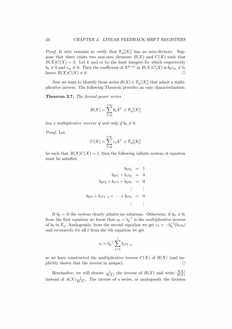
Now we want to identify those series B(X) ∈ Fq[[X]] that admit a multi-plicative inverse. The following Theorem provides an easy characterization.
Theorem 2.7. The formal power series
B(X) =+∞∑t=0
btXt ∈ Fq[[X]]
has a multiplicative inverse if and only if b0 6= 0.
Proof. Let
C(X) =+∞∑t=0
ctXt ∈ Fq[[X]]
be such that B(X)C(X) = 1, then the following infinite system of equationmust be satisfied
b0c0 = 1
b0c1 + b1c0 = 0
b0c2 + b1c1 + b2c0 = 0...
...
b0ct + b1ct−1 + · · ·+ btc0 = 0...
...
If b0 = 0 the system clearly admits no solutions. Otherwise, if b0 6= 0,from the first equation we know that c0 = b−1
0 is the multiplicative inverseof b0 in Fq. Analogously, from the second equation we get c1 = −b−1
0 (b1c0)and recursively for all t from the tth equation we get
ct = b−10
t∑j=1
bjct−j
so we have constructed the multiplicative inverse C(X) of B(X) (and im-plicitly shown that the inverse in unique).
Hereinafter, we will denote 1B(X) the inverse of B(X) and write A(X)
B(X)
instead of A(X) 1B(X) . The inverse of a series, or analogously the division

2.1. LINEAR RECURRING SEQUENCES IN FQ 25
between two series, can be computed in the usual way. Simply in most casesthe algorithm will be infinite.
Now let’s show a basic identity for the generating function of a givensequence.
Theorem 2.8. Let stt∈N be a Lth-order homogeneous linear recurringsequence over Fq satisfying 2.1.2. Let f∗(X) ∈ Fq[X] be its feedback poly-nomial and G(X) ∈ Fq[[X]] be its generating function as defined in 2.1.7.Then the identity
G(X) =g(X)
f∗(X)(2.1.9)
holds with
g(X) = −L−1∑j=0
j∑i=0
ai+L−jsiXj ∈ Fq[X] (2.1.10)
where we set aL = −1.
Conversely, if g(X) is any polynomial over Fq with deg(g) < L andif f∗(X) ∈ Fq[X] is given by 2.1.4, then the formal power series G(X) ∈Fq[[X]] defined by 2.1.9 is the generating function of a Lth-order homoge-neous linear recurring sequence in Fq satisfying the linear recurrence relation2.1.2.
Proof. First, we have
f∗(X)G(X) = −
(L∑t=0
aL−tXt
)(+∞∑t=0
stXt
)=
= −L−1∑j=0
(j∑i=0
ai+L−jsi
)Xj −
+∞∑j=L
j∑i=j−L
ai+L−jsi
Xj =
= g(X)−+∞∑j=L
(L∑i=0
aisj−L+i
)Xj (2.1.11)
Since st satisfies 2.1.2, for every j ≥ L we can take t = j − L in 2.1.2obtaining
L∑i=0
aisj−L+i = 0
Thus 2.1.11 becomes
f∗(X)G(X) = g(X)
and, since f∗(X) admits a multiplicative inverse in Fq[[X]], the identity 2.1.9follows.

26 CHAPTER 2. LINEAR FEEDBACK SHIFT REGISTERS
Conversely, from 2.1.11 we infer that f∗(X)G(X) is equal to a polynomialof degree less than L if and only if
L∑i=0
aisj−L+i = 0 for all j ≥ L
But these identities just express the fact that the sequence st of the coef-ficients of G(X) satisfies the linear recurrence relation 2.1.2.
We can summarize Theorem 2.8 by saying that the Lth-order homo-geneous linear recurring sequences with feedback polynomial f∗(X) are in
one-to-one correspondence with the fractions g(X)f∗(X) with deg(g) < L, where
every choice of the initial state of the sequence entails the choice of g(x) asdefined in 2.1.10. The identity 2.1.9 permits to compute the terms of thesequence with that initialization by long division.
Example 2.7. Consider the linear recurrence relation
st+4 = st+3 + st+1 + st
over F2, whose feedback polynomial is
f∗(X) = 1−X −X3 −X4 = 1 +X +X3 +X4 ∈ F2[X]
If the initial state is (1, 1, 0, 1), we have g(X) = 1 + X2 and by longdivision we compute
G(X) =1 +X2
1 +X +X3 +X4= 1 +X +X3 +X4 +X6 + · · ·
which corresponds to the sequence 1, 1, 0, 1, 1, 0, 1, . . . of least period 3.Otherwise, if we take the impulse response sequence, whose initial state
is (0, 0, 0, 1), we have g(X) = X3 and
G(X) =X3
1 +X +X3 +X4= X3 +X4 +X5 +X9 +X10 +X11 + · · ·
which corresponds to the sequence 0, 0, 0, 1, 1, 1, 0, 0, 0, 1, 1, 1, . . . of leastperiod 6.
Thanks to identity 2.1.9 we can give a proof of Theorem 2.3. Sincethe sequence st is periodic with period r, its generating function can bewritten as
G(X) = (s0 + s1X + · · ·+ sr−1Xr−1)(1 +Xr +X2r + · · · ) =
s∗(X)
1−Xr
where we called s∗(X) = s0 +s1X+· · ·+sr−1Xr−1 and we noted that 1−Xr
is the multiplicative inverse of 1 +Xr +X2r + · · · .

2.1. LINEAR RECURRING SEQUENCES IN FQ 27
Equating this expression with identity 2.1.9, we get
g(X)
f∗(X)=
s∗(X)
1−Xr
or equivalentlys∗(X)f∗(X) = (1−Xr)g(X)
Now, if we recall the relation between characteristic and feedback polyno-mial of a sequence
(f∗(X) = XLf
(1X
))and if we note that an analogous
relation exists between s∗(X) and the polynomial s(X) defined in Theorem2.3
(s∗(X) = Xr−1s
(1X
)), we get
s∗(X)f∗(X) = Xr−1s
(1
X
)XLf
(1
X
)= (1−Xr)g(X)
which implies
s
(1
X
)f
(1
X
)=
1−Xr
Xr
1
XL−1g(X) =
(1
Xr− 1
)1
XL−1g(X)
⇔ s(X)f(X) = (Xr − 1)XL−1g
(1
X
)and noting that, if h(X) is defined as in Theorem 2.3,
XL−1g
(1
X
)= −h(X) (2.1.12)
leads to the desired conclusion.
The following Theorem finally describes the relation between the differ-ent linear recurrence relations valid for a given homogeneous linear recurringsequence.
Theorem 2.9. Let stt∈N be a linear recurring sequence over Fq. Then,there exists a uniquely determined monic polynomial m(X) ∈ Fq[X] suchthat every other monic polynomial f(X) ∈ Fq[X] of positive degree is acharacteristic polynomial of st if and only if m(X) divides f(X).
Proof. Let f0(X) ∈ Fq[X] be the characteristic polynomial of a homogeneouslinear recurrence relation satisfied by the sequence. We know that, if thesequence is periodic with period r, we can write f0(X)s(X) = (1−Xr)h0(X),where the polynomials s(X) and h0(X) are defined as in Theorem 2.3. Now,if d(X) is the (monic) greatest common divisor of f0(X) and h0(X), we canwrite f0(X) = d(X)m(X) and h0(X) = b(X)d(X), with m(X), b(X) ∈Fq[X]. We shall prove that m(X) is the desired polynomial.
Clearly m(X) is monic and divides f0(X). Now, let f(X) be any othercharacteristic polynomial of the sequence and h(X) be the corresponding

28 CHAPTER 2. LINEAR FEEDBACK SHIFT REGISTERS
polynomial in Theorem 2.3. By applying Theorem 2.8, we obtain that theganerating function G(X) of the sequence satisfies
G(X) =g0(X)
f∗0 (X)=
g(X)
f∗(X)
with g0(X) and g(X) determined by 2.1.10. Therefore
g0(X)f∗(X) = g(X)f∗0 (X)
and using 2.1.12 we get
h(X)f0(X) = −Xdeg(f)−1g
(1
X
)Xdeg(f0)f∗0
(1
X
)=
= −Xdeg(f0)−1g0
(1
X
)Xdeg(f)f∗
(1
X
)= h0(X)f(X)
so now, dividing by d(X) entails
h(X)m(X) = b(X)f(X)
Since, by definition of d(X), m(X) and b(X) are relatively prime, thennecessarily m(X) divides f(X).
Conversely, suppose that f(X) ∈ Fq[X] is a monic polynomial of positivedegree and that it is divisible by m(X), say f(X) = c(X)m(X) with c(X) ∈Fq[X]. Passing to reciprocal polynomials, we have f∗(X) = c∗(X)m∗(X).Furthermore, clearly h0(X)m(X) = b(X)f0(X). Now, using 2.1.12 we get
g0(X)m∗(X) = −Xdeg(f0)−1h0
(1
X
)Xdeg(m)m
(1
X
)=
= −Xdeg(m)−1b
(1
X
)Xdeg(f0)f0
(1
X
)= −Xdeg(m)−1b
(1
X
)f∗0 (X)
Note that, since deg(h0) < deg(f0), then deg(c) < deg(m), so the product−Xdeg(m)−1b
(1X
)is a polynomial a(X) ∈ Fq[X]. Then we can write
g0(X)m∗(X) = a(X)f∗0 (X)
and multiplying for c∗(X) we get
g0(X)f∗(X) = a(X)f∗0 (X)c∗(X)
or analogously, dividing by f∗0 (X)f∗(X) and recalling the definition of G(X),
G(X) =g0(X)
f∗0 (X)=a(X)c∗(X)
f∗(X)
2.1. LINEAR RECURRING SEQUENCES IN FQ 29
Since
deg(a · c∗) = deg(a) + deg(c∗) < deg(m) + deg(c) = deg(f)
the second part of Theorem 2.8 shows that f(X) is a characteristic polyno-mial of the sequence.
Finally, by the way we have defined m(X) it is clearly uniquely deter-mined.
Definition 2.8. The uniquely determined polynomial m(X) of Theorem2.9 is called the minimal polynomial of the sequence.
If st = 0 for all t ≥ 0, the minimal polynomial is equal to the constantpolynomial 1, while for any other homogeneous linear recurring sequencem(X) is a monic polynomial with deg(m) > 0. Note that the minimalpolynomial of a linear recurring sequence is the characteristic polynomial ofthe linear recurrence relation of least possible order satisfied by the sequence.
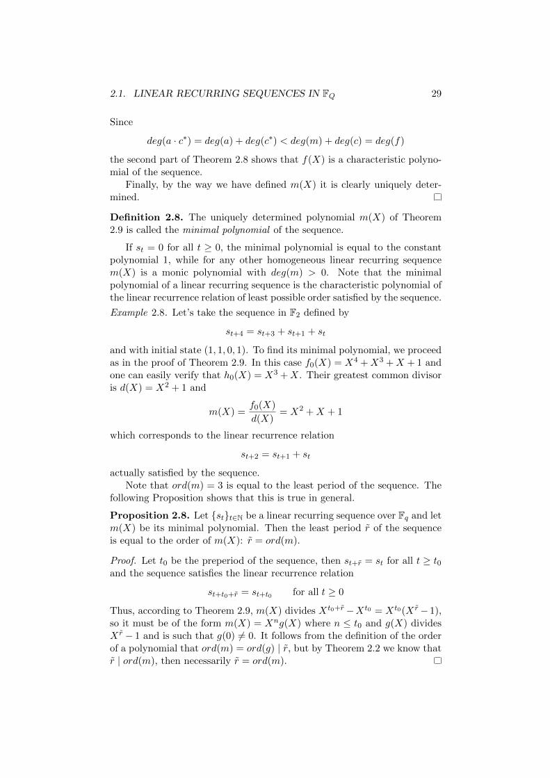
Example 2.8. Let’s take the sequence in F2 defined by
st+4 = st+3 + st+1 + st
and with initial state (1, 1, 0, 1). To find its minimal polynomial, we proceedas in the proof of Theorem 2.9. In this case f0(X) = X4 +X3 +X + 1 andone can easily verify that h0(X) = X3 +X. Their greatest common divisoris d(X) = X2 + 1 and
m(X) =f0(X)
d(X)= X2 +X + 1
which corresponds to the linear recurrence relation
st+2 = st+1 + st
actually satisfied by the sequence.Note that ord(m) = 3 is equal to the least period of the sequence. The
following Proposition shows that this is true in general.
Proposition 2.8. Let stt∈N be a linear recurring sequence over Fq and letm(X) be its minimal polynomial. Then the least period r of the sequenceis equal to the order of m(X): r = ord(m).
Proof. Let t0 be the preperiod of the sequence, then st+r = st for all t ≥ t0and the sequence satisfies the linear recurrence relation
st+t0+r = st+t0 for all t ≥ 0
Thus, according to Theorem 2.9, m(X) divides Xt0+r−Xt0 = Xt0(X r− 1),so it must be of the form m(X) = Xng(X) where n ≤ t0 and g(X) dividesX r − 1 and is such that g(0) 6= 0. It follows from the definition of the orderof a polynomial that ord(m) = ord(g) | r, but by Theorem 2.2 we know thatr | ord(m), then necessarily r = ord(m).

30 CHAPTER 2. LINEAR FEEDBACK SHIFT REGISTERS
Now we can find the least period of a linear recurring sequence withoutevaluating its terms, as shown in the following example. The method isparticularly effective if a table of orders of polynomials is available.
Example 2.9. Let’s take the sequence in F2 defined by
st+5 = st+1 + st
with initial state (1, 1, 1, 0, 1) and proceed as in the proof of Theorem 2.9.In this case f0(X) = X5 +X+ 1, h0(X) = X4 +X3 +X2 and their greatestcommon divisor is d(X) = X2 + X + 1. Then the minimal polynomial ofthe sequence is
m(X) =f0(X)
d(X)= X3 +X2 + 1
whose order is 7, which we know to coincide with the least period of thesequence.
Proposition 2.9. Let f(X) ∈ Fq[X] be monic and irreducible over Fq andlet st be a homogeneous linear recurring sequence in Fq not all of whoseterms are 0. If f(X) is a characteristic polynomial of the sequence, then itis its minimal polynomial.
Proof. It follows easily from 2.9. In fact, since the minimal polynomialm(X)of the sequence divides f(X), the irreducibility of f(X) implies that eitherm(X) = 1 or m(X) = f(X). But m(X) = 1 holds only for the sequence allof whose terms are 0, so necessarily m(X) = f(X).
Anyhow, a characteristic polynomial can be the minimal polynomial of asequence even if it is not irreducible. The following Theorem gives a generalcriterion to verify it.
Theorem 2.10. Let stt∈N be a sequence in Fq satisfying a Lth-order ho-mogeneous linear recurrence relation with characteristic polynomial f(X) ∈Fq[X]. Then f(X) is the minimal polynomial of the sequence if and only ifthe state vectors s0, s1, . . . , sL−1 are linearly independent over Fq.
Proof. First, suppose f(X) is the minimal polynomial of the sequence. Ifthere existed coefficients b0, b1, . . . , bL−1 ∈ Fq not all of which are 0 suchthat b0s0 + b1s1 + · · ·+ bL−1sL−1 = 0, we could multiply from the right bypowers of the matrix A associated with f(X), obtaining
b0st + b1st+1 + · · ·+ bL−1st+L−1 = 0 for all t ≥ 0
In particular we would have
b0st + b1st+1 + · · ·+ bL−1st+L−1 = 0 for all t ≥ 0

2.1. LINEAR RECURRING SEQUENCES IN FQ 31
which define a new linear recurrence relation satisfied by the sequence. Now,bj = 0 for all 1 ≤ j ≤ L − 1 implies st = 0 for all t ≥ 0, which contradictsthe assumption that the minimal polynomial of the sequence is f(X), whosedegree is L. So, let j ≥ 1 be the largest index with bj 6= 0. Then the sequenceclearly satisfies a jth-order homogeneous linear recurrence relation with j <L, which again contradicts the assumption that the minimal polynomial ofthe sequence is f(X). Therefore, we have shown that s0, s1, . . . , sL−1 arelinearly independent over Fq.
Conversely, suppose that s0, s1, . . . , sL−1 are linearly independent overFq. Since s0 6= 0, the minimal polynomial has positive degree. If f(X)were not the minimal polynomial, the sequence would satisfy a recurrencerelation of order m with 1 ≤ m < L. But this eventuality is impossible,since if
st+m = bm−1st+m−1 + · · ·+ b0st for all t ≥ 0
for some coefficients b0, . . . , bm−1 ∈ Fq, then the same identity is true for thestate vectors s0, s1, . . . , sm, contradicting the assumption of linear indepen-dence.
Corollary 1. Let (d,a) be an impulse response sequence over Fq. Thenits minimal polynomial coincides with the characteristic polynomial of thelinear recurrence relation defined by the vector a.
Proof. The results follows trivially from Theorem 2.10, since the requiredlinear independence property is obviously satisfied by the initial states of animpulse response sequence.
Example 2.10. Let’s go back in F25 as in example 2.3.
This time let’s take the recurrence relation st+2 = st+1 + st, whose char-acteristic polynomial is f(X) = X2 − X − 1, which is reducible over F5,being X2 − X − 1 = (X − 3)2. F2
5 is divided in 3 orbits: one obviouslycontains only (0, 0), while the remaining 24 elements form two orbits with 4and 20 elements respectively. The minimal polynomial of the shortest orbitis the constant polynomial m0(X) = 1. The longest orbit corresponds to theimpulse response sequence and, as stated by corollary 1, its minimal poly-nomial is f(X). The last orbit corresponds to the sequence 1, 3, 4, 2, 1, 3, . . .and its minimal polynomial is m(X) = X − 3; in fact, as the reader caneasily check, it satisfies the shorter linear recurrence relation st+1 = 3st.
Finally, we give a definition which applies to every sequence in a finitefield Fq. It resumes somehow the characterization of a sequence given thusfar, describing its pseudo-randomness and the difficulty of recreating it orpredicting its next digit.
Definition 2.9. Let stt∈N be a generic sequence over Fq. We defineits linear complexity as the order of the shortest linear recurrence relation

32 CHAPTER 2. LINEAR FEEDBACK SHIFT REGISTERS
satisfied by the sequence, namely the degree of its minimal polynomial. Ifthe sequence does not satisfy any linear recurrence relation, we say its linearcomplexity to be ∞, while the linear complexity of the all-zero sequence is0.
2.2 Combining linear recurring sequences
Although we have seen how to generate linear recurring sequences withmaximal linear complexity and period, that’s not enough to build a strongstream cipher. If we used the output of a LFSR as a keystream, the ci-pher would be weak under many attacks, in the first place one mountedusing Berlekamp-Massey’s algorithm. That algorithm, invented by ElwynBerlekamp in 1968, is in fact able to find the minimal polynomial of a linearrecurring sequence in time O(Λ) knowing only 2Λ consecutive digits, whereΛ is the linear complexity of the sequence.
Furthermore, a linear recurring sequence couldn’t be directly used as akeystream anyway, since, even if it has interesting randomicity properties,it also has very strong linearity properties. Combining it directly to theplaintext wouldn’t supply any security against the so-called algebraic attacks,that recover the key of a cipher by formulating and solving a system of linearequations.
A known-plaintext attack2, in particular, would be very simple to imple-ment and very effective. According to Kerckhoffs’ principle, we can supposethe attacker to know the structure of the LFSR, namely its length L andfeedback relation st+L =
∑L−1i=0 aist+i. His aim is hence finding the initial
state of the register, which is actually the key of the cipher. If he knows anyL plaintext digits mt1 , . . . ,mtL and the corresponding ciphertext digits, hecan formulate the trivial system
ctj = stj +mtj
j = 1, . . . , L
Recalling the recurrence relation of the sequence st, each digit stj can bewritten as a linear combination of the key, so the system becomes a systemof L linear equations in the L unknowns s0, . . . , sL−1, solvable in O(L3)operations with Gauss’ algorithm.
Many other very incisive similar attacks could be moved, so we needto shatter the linearity of the sequence and make it unexploitable by thecryptanalysts.
The natural solution to these two problems, increasing the linear com-plexity of the sequence and shattering its linearity, consists in combining
2A known-plaintext attack is an attack mounted knowing some couples of plaintextand corresponding ciphertext

2.2. COMBINING LINEAR RECURRING SEQUENCES 33
n registers in parallel through a non-linear function f : Fnq → Fq, calledcombining function.
This approach further strengthens the cipher involving a considerableincrease of the keyspace, since the key of such a cipher is no longer theinitialization of a register, but those of n different registers.
The scheme of this kind of ciphers is shown in figure 4.1.
Figure 2.2: A typical LFSR combination generator
Si = sitt∈N denotes the output of the ith register, while the output off is the keystream Y = ytt∈N, which is usually added digit by digit withthe plaintext M = mtt∈N to generate the ciphertext C = ctt∈N.
In the previous section we studied how the choice of a LFSR and itsinitialization affects the properties of the linear recurring sequence generatedby it. We are now going to do the same work for the sequence Y : detectits properties and comprehend how they depend on the LFSRs and on thecombining function f .
Even if Y is not directly generated by a LFSR, we can still talk of itsperiod and linear complexity, since these two notions are defined for anysequence in a finite field Fq. Furthermore, if we call N the keystream’stotal length, we can always imagine Y to be generated by a register whosecharacteristic polynomial is g(X) = XN − 1 and thus take N as an upperbound for both its period and its linear complexity. What we want to do isto actually ensure that it does not exist a polynomial of lower degree thatcould have generated Y .
2.2.1 Multivariate functions over finite fields
When talking about multivariate functions over a finite field Fq, first of allwe need the to introduce a fundamental instrument.
Definition 2.10. Let f : Fnq → Fq be any function in n unknowns over Fq.f can always be represented as a multivariate polynomial called its Algebraic
34 CHAPTER 2. LINEAR FEEDBACK SHIFT REGISTERS
Normal Form. The ANF of f is the only polynomial
Qf ∈Fq[X1, . . . , Xn]
(Xq1 −X1, . . . , X
qn −Xn)
such thatf(x) = Qf (x) for all x = (x1, . . . , xn) ∈ Fnq
The degree of f is then defined as the total degree of the polynomial Qf :deg(f) = deg(Qf ).
This representation, which could seem not so natural at first sight, isactually very simple. It just exploits the fact that every function f : Fnq →Fq, assuming only q values, must be formulable as a polynomial and, sinceXq ≡ X in Fq, every variable can appear in the polynomial form of f onlywith degree not greater than q − 1. Hence we can write the ANF of f as
Qf =∑u∈Fnq
auXu
where we used the notation Xu = Xu11 · · ·Xun
n and we assumed that 00 = 1.From here on, we will automatically suppose any function to be expressed
through its ANF.Thanks to the polynomial representation of the combining function, we
can see the generic keystream digit yt as the result of a combination of sumsand products on the corresponding digits sit. This allows us to describeY just defining the operations of sum and product of two linear recurringsequences and their properties.
Boolean functions
When q = 2, the functions from the set Fn2 of n-bit words into F2 are calledboolean functions.
In practical applications, this case is obviously the most frequent one.Boolean functions have been thus deeply analyzed in literature and the par-ticularly simple structure of F2 permitted a refined characterization of thosefunctions.
Let f : Fn2 → F2 be any boolean function, we usually represent f throughits ANF:
f(X) =∑u∈Fn2
auXu (2.2.1)
Note that this time every variable Xi can appear only with degree 1.
Let u = (u1, . . . , un) ∈ Fn2 be any vector, we call its support, denotedsupp(u), the set of its non-zero components. supp(u) tells us which vari-ables appear in the corresponding monomial Xu. If u = (01101) ∈ F5
2, forexample, then supp(u) = 2, 3, 5 and Xu = X2X3X5.

2.2. COMBINING LINEAR RECURRING SEQUENCES 35
If we divide f(X) by any monomial Xu, we obtain
f(X) = Xu(au + pu(X)) + ru(X) = auXu +Xupu(X) + ru(X)
where pu(X) is a polynomial with free term 0.A term Xv is divisible by Xu if and only if supp(u) ⊆ supp(v), namely
if and only if Xv = Xu ·Xi1 · · ·Xik for some indices i1, . . . , ik ∈ 1, . . . , n \supp(u).
Hence any monomial of pu(X) can’t contain any variable appearing inXu, while a monomial in ru(X) can contain some of the variables in supp(u),but obviously there must be at least one it does not contain.
Proposition 2.10. Let f : Fn2 → F2 be any boolean function expressed inits ANF 2.2.1. It holds
au =⊕xu
f(x) for all u ∈ Fn2 (2.2.2)
where denotes the partial order on Fn2 defined by “v u if and only ifvi ≤ ui for all i = 1, . . . , n”. Namely, v u if and only if supp(v) ⊆ supp(u).
Proof. Let x be any vector such that x u.
• Since supp(x) ⊆ supp(u), any 1 in x is in a position corresponding toa variable actually appearing in Xu, hence a variable not appearingin any monomial of pu(X). This means clearly that pu(x) = 0 andconsequently
⊕xu x
upu(x) =⊕
xu 0 = 0.
• Take any monomial in ru(X), say Xv. We have shown that necessarilysupp(u) 6⊆ supp(v), so let i ∈ supp(u) \ supp(v) and hence Xi beany variable appearing in Xu but not in Xv. Since i ∈ supp(u),if we take the vector x′ obtained by x flipping its i-th bit, clearlyalso x′ u. But, since i /∈ supp(v), clearly the monomial Xv takesthe same value when evaluated on x and x′. More generally, everymonomial in ru(X) takes the same value on an even number of vectorsx u, thus
⊕xu ru(x) = 0.
• Finally, Xu is worth 1 if and only if it is evaluated on a vector x suchthat supp(u) ⊆ supp(x), but the only vector x u with this propertyis u itself. Hence,
⊕xu x
u = 1.
Now trivially⊕xu
f(x) =⊕xu
(auxu + xupu(x) + ru(x)) =
= au⊕xu
xu +⊕xu
xupu(x) +⊕xu
ru(x) = au

36 CHAPTER 2. LINEAR FEEDBACK SHIFT REGISTERS
Example 2.11. Take the function
f(X1, X2, X3, X4) = X2 +X2X3 +X1X2X3 +X2X3X4 + 1
If u = (0110), Xu = X2X3 and obviously au = 1. We can easily verify theProposition:⊕
xuf(x) = f(0000) + f(0100) + f(0010) + f(0110) =
= 1 + 0 + 1 + 1 = 1
Furthermore, let’s practically see what we have said in the proof:
f(X) = X2X3(1 +X1 +X4) + 1 +X2 =
= X2X3 +X2X3(X1 +X4) + (1 +X2)
and ⊕xu
x2x3(x1 + x4) = 0 + 0 + 0 + 0 = 0
⊕xu
(1 + x2) = 1 + 0 + 1 + 0 = 0
⊕xu
x2x3 = 0 + 0 + 0 + 1 = 1
Another way to describe a boolean function is to identify it with itstruth table. The sets of functions from Fn2 into F2 is in fact in one-to-onecorrespondence with the set F2n
2 .The correspondence is built by simply associating to any function f its
truth table, namely the ordered sequence of the values taken by f on theelements of Fn2 . The order in the sequence is induced by the order chosenfor the set Fn2 , such as the natural one obtained considering any x ∈ Fn2 asthe binary representation of a number between 0 and 2n − 1.
According to the previous definition, supp(f) should denote the set ofthe non-zero components in f ’s truth table. Anyhow, it is usually used inthe classical meaning of the set x ∈ Fn2 : f(x) 6= 0. Substantially, thetwo definitions agree, since any 1 in f ’s truth table correspond to a vectorx such that f(x) 6= 0.
Thanks to this different perspective, we can extend to boolean functionsthe notions of Hamming weight and distance, defined for vectors in Fn2 forall n.
Definition 2.11. Let u, v ∈ Fn2 be two vectors. The Hamming weight of u,denoted wH(u), is defined as the number of its non-zero components, namelythe cardinality of supp(u):
wH(u) = |i : ui = 1|

2.2. COMBINING LINEAR RECURRING SEQUENCES 37
The Hamming distance between u and v, denoted dH(u, v), is the numberof components in which the two vectors differ, namely the Hamming weightof their bitwise modular sum:
dH(u, v) = |i : ui 6= vi| = |i : ui ⊕ vi = 1|
Now, given two functions f and g, we can naturally talk of wH(f) anddH(f, g), implicitly referring to their truth tables. It holds
dH(f, g) =∑x∈Fn2
(f + g)
A very useful instrument to study boolean functions from this point ofview is the Walsh-Hadamard transform.
Definition 2.12. Let f : Fn2 → F2 be any boolean function. We define itsWalsh-Hadamard transform as the Fourier transform of the correspondingsign function, ϕf : x 7→ (−1)f(x), with respect to the representation ψu :x 7→ (−1)u·x:
for all u ∈ Fn2 χf (u) =∑x∈Fn2
(−1)f(x)(−1)u·x (2.2.3)
We recall that any function g of the form g(x) = u · x+ ε, where u ∈ Fn2and ε ∈ F2, is called affine.
The Fourier transform of a function ϕ : Fn2 → C at a representationψ : Fn2 → C is defined as
ϕ(ψ) =∑x∈Fn2
ϕ(x)ψ(x) = 〈ϕ,ψ〉
The idea is to build a new instrument to compare f(x) with the affinefunctions u · x for all u ∈ Fn2 , which does not work anymore in modulararithmetic. Hence we need a function that can take a number of differentvalues equal to the number of possible values of f(x)− u · x.
The solution in the binary case is to take the primitive square root ofunity, -1, and raise it to the difference between f(x) and u ·x. This time theobtained function is particularly useful because it takes values in R.
If we fix u ∈ Fn2 , the generic term of the sum in 2.2.3 is
(−1)f(x)+u·x =
+1 if f(x) = u · x−1 if f(x) 6= u · x
that can be written as 1−2(f(x)+u·x). It follows that χf (u) varies between2n, when f(x) = u · x for all x ∈ Fn2 , and −2n, when f(x) = u · x+ 1 for all

38 CHAPTER 2. LINEAR FEEDBACK SHIFT REGISTERS
x ∈ Fn2 , and it’s 0 if f(x) and u · x coincide on exactly half of the possibleinputs.
It is then clear that χf (u) estimates the Hamming distance between fand the affine functions u · x+ ε. More precisely
χf (u) =∑x∈Fn2
(−1)f(x)+u·x
= (−1)ε∑x∈Fn2
(−1)f(x)+u·x+ε
= (−1)ε∑x∈Fn2
(1− 2(f(x) + u · x+ ε))
= (−1)ε
2n − 2∑x∈Fn2
(f(x) + u · x+ ε)
= (−1)ε(2n − 2dH(f, u · x+ ε))
hence
dH(f, u · x+ ε) = 2n−1 − (−1)ε
2χf (u) (2.2.4)
The Walsh spectrum of a boolean function completely characterize it, asshown by the following Proposition.
Proposition 2.11. Let f : Fn2 → F2 be any boolean function describedthrough its ANF as in 2.2.1.
Hence, for all u ∈ Fn2 it holds
au = 2wH(u)−1
1− 1
2n
∑vu
χf (u)
mod 2 (2.2.5)
where u denotes the bitwise completion of u, i.e. ui = 1 if and only if ui = 0.
Proof. Thanks to equation 2.2.2 we get
au =∑xu
f(x) mod 2 =∑xu
1
2(1− (−1)f(x)) mod 2
=1
2|x u| − 1
2
∑xu
(−1)f(x) mod 2
= 2wH(u)−1 − 1
2
∑xu
(−1)f(x) mod 2
Since the normalized Fourier transform is involutive, it holds
for all x ∈ Fn2 , (−1)f(x) = 2−n∑v∈Fn2
χf (v)(−1)v·x

2.2. COMBINING LINEAR RECURRING SEQUENCES 39
Now, combining these two results, we have
au = 2wH(u)−1 − 2−n−1∑xu
∑v∈Fn2
χf (v)(−1)v·x mod 2
= 2wH(u)−1 − 2−n−1∑v∈Fn2
χf (v)
∑xu
(−1)v·x
mod 2
The set Eu = x ∈ Fn2 : x u is a linear subspace of Fn2 of dimensionwH(u). Its orthogonal E⊥u clearly satisfies E⊥u = Eu, hence∑
xu(−1)v·x =
2wH(u) if v ∈ Eu0 otherwise
In fact, if v /∈ Eu, there must exist an index i such that vi = ui = 1. Hence,for any x ∈ Eu, the vector x′ ∈ Eu obtained flipping the ith bit of x satisfiesv · x 6= v · x′ and consequently (−1)v·x + (−1)v·x
′= 0. Now finally
au = 2wH(u)−1 − 2−n−1+wH(u)∑vu
χf (v) mod 2
In this context, boolean functions are used in keystream generators tocombine the outputs of some LFSR, thus we want them to have some prop-erties essential to resist to some known attacks.
Since the main purpose is shattering the linearity of linear recurring se-quences, we want the combining function to be definitely non-linear, namelyto be as “far” as possible to any affine function.
At first sight, one could imagine to simply look at the total degree of afunction, since the higher is deg(f) the most f is supposed to act differentlyfrom any linear combination. If deg(f) is high, in fact, some monomials in fdepends on many of its input at the same time, making apparently difficultany algebraic attack.
This is a proper remark, but what we actually need most is to be surethat, given any linear combination g(x) = u · x, f ’s truth table does notcoincide too much neither with g or with g + 1.
Suppose, in fact, that f coincides with g on 90% of the possible inputs.Many statistical attacks could be mounted by simply supposing that thecombining function used is actually g, but that with probability 1
10 theciphertext bit we have at our disposal is wrong.
The best way to measure how far a function f is from being linear ishence to define its nonlinearity as its minimum distance from any affinefunction:
nl(f) := ming(x)=u·x+ε
dH(f, g)

40 CHAPTER 2. LINEAR FEEDBACK SHIFT REGISTERS
Thanks to identity 2.2.4, we can alternatively define it as
nl(f) = 2n−1 − 1
2maxu∈Fn2
|χf (u)| (2.2.6)
Note that, if f and g are two functions from Fn2 into F2, dH(f, g) =2n−dH(f, g+1), hence evaluating dH(f, g) or dH(f, g+1) is equivalent andonly one of the two calculation is necessary.
When g is constant, say g(x) ≡ 0 (but g(x) ≡ 1 would be clearly equiva-lent), we talk of a more particular and basic property of boolean functions,called balance.
A function f : Fn2 → F2 is balanced if its output is uniformly distributed,namely if P (f = 0) = P (f = 1) = 1
2 . The probability is usually simplyintended as
P (f = ε) =|x ∈ Fn2 : f(x) = ε|
2n
hence f is balanced if and only if wH(f) = 2n−1.The importance of this property is evident thanks to Shannon’s entropy,
as shown in the example.
Example 2.12. Suppose a combining function f is unbalanced, say p0 =P (f = 0) = 1
4 and p1 = P (f = 1) = 34 . The entropy of the keystream Y is
H(Y ) = p0 · log2
1
p0+ p1 · log2
1
p1
=1
4· log2 4 +
3
4· log2
4
3
=1
2+
3
2− 3
4· log2 3 = 2− 3
4· log2 3 > 1
hence the generic keystream bit yt carries more than a bit of information.The value taken by yt depends on the output at time t of the n LFSRs
and allows to understand if the n-tuple belongs to a set of 2n
4 elements oris one of the remaining 3·2n
4 . That’s why the amount of information carriedby yt is different from the one carried by a random bit. In particular, theresult highlights that the gain in information when yt = 0 is bigger than theloss when yt = 1.
Note that, any time the plaintext is unbalanced, the same property istransmitted to the ciphertext, and that’s obviously a problem.
The balance property can be easily expressed through the Walsh coeffi-cients, since clearly a function f is balanced if and only if χf (0) = 0.
The property of a function to be statistically independent from linearcombinations of its inputs was precisely defined by Siegenthaler in [16].
Definition 2.13. A boolean function f is t-th order correlation-immune ifthe probability distribution of its output is unaltered when the values of anyt input variables are fixed.

2.2. COMBINING LINEAR RECURRING SEQUENCES 41
The definition equivalently asserts that the output of f is statisticallyindependent from any linear combination of t of its input variables. Asany other property, the correlation immunity order of a function can becharacterized by its Walsh spectrum. In fact
P (f(x) = u · x) =|x ∈ Fn2 : f(x) = u · x|
2n
=2n − dH(f, u · x)
2n
=2n − 2n−1 + 2−1χf (u)
2n
=2n−1 + 2−1χf (u)
2n
=1
2+χf (u)
2n+1
namely
P (f(x) = u · x) =1
2
(1 +
χf (u)
2n
)(2.2.7)
The following Proposition is now trivial.
Proposition 2.12. Let f be any boolean function. f is t-th order correlation-immune if and only if
χf (u) = 0 for all u ∈ Fn2 such that 1 ≤ wH(u) ≤ t
Proof. f is t-th order correlation-immune if and only if P (f(x) = u · x) = 12
for all u ∈ Fn2 such that 1 ≤ wH(u) ≤ t. Thus the conclusion follows easilyfrom equation 2.2.7.
Since any t-th order correlation-immune function is also k-th order correlation-immune for any k ≤ t, we call correlation-immunity order of a function fthe largest t such that f is t-th order correlation-immune.
A function f is finally called t-resilient when f is balanced and itscorrelation-immunity order is t.
Expressing the cryptographic properties of a boolean function throughthe properties of its Walsh spectrum highlights the necessity of a trade-offamong them.
Parseval’s Theorem, which applies to any Fourier transform, states that∑x∈Fn2
((−1)f(x)
)2=
1
|Fn2 |∑u∈Fn2
(χf (u))2
which means ∑u∈Fn2
(χf (u))2 = 2n∑x∈Fn2
1 = 22n

42 CHAPTER 2. LINEAR FEEDBACK SHIFT REGISTERS
Hence the Walsh coefficients of a function f can’t be all 0 and the biggeris the number of null ones, the bigger the non-null ones are in absolute value.Consequently, the higher is the correlation-immunity order of f , the biggermaxu∈Fn2 |χf (u)| is supposed to be, hence the lower may be f ’s nonlinearity.
Furthermore, the following (quite trivial) results holds [16]:
• the correlation-immunity order of a function f with n variables isclearly bounded by n − 1 and if f ’s correlation-immunity order is t,then deg(f) ≤ n− t
• if f is t-resilient, then
– if t ≤ n− 2, it holds deg(f) ≤ n− t− 1
– if t = n− 1, it holds deg(f) = 1
Finally, if we want the cipher to be fairly strong under any type of attack,the best we can aspire to is hence a combining function with correlation-immunity order t not too low and such that |χf (u)| = c for all u withwH(u) > t, where c is a constant.
Let’s now come back to the general case of any finite field Fq.The functions from Fnq into Fq and their properties have not been deeply
analyzed in literature, since the q-nary case is probably considered moreinteresting in theory than practice.
Anyhow, the notions of nonlinearity and correlation-immunity order canbe extended to any function f : Fnq → Fq and they have the identicalmeaning.
The main difference with the binary case is that Proposition 2.10 can’t beextended, since that result follows from the fact that a variable can appearin the ANF of a boolean function only with degree 1.
Furthermore, the main instrument that allowed us to characterize theboolean functions having a particular property and to understand whichproperties are compatible is the Walsh spectrum of the function. Unfortu-nately, it can be defined only for the finite fields Zp of prime cardinality andanyway many of its properties are not valid anymore.
The idea of the Walsh coefficients is somehow to transform an additivegroup in a multiplicative one. If f : Fnq → Fq and u ∈ Fnq , the differencef(x)− u · x can take q different values. To build a complex-valued functionwhich can take those q values, we should take the q-th root of unity ω =
e2πiq ∈ C and elevate it to the integer associated to f(x)−u ·x. But ωf(x)−u·x
corresponds to the product ωf(x) ·ω−u·x only if Fq is a cyclic group with thesum and this is true if and only if q = p is prime.
This means that the Walsh-Hadamard transform of f can be usefullydefined only for Zp as the Fourier transform of ϕf : x 7→ ωf(x) at the

2.2. COMBINING LINEAR RECURRING SEQUENCES 43
representation ψu : x 7→ ωu·x, namely as
χf (u) =∑x∈Znp
ωf(x)ωu·x =∑x∈Znp
ωf(x)−u·x
where we have used ω = e− 2πi
q = ω−1.Unlike the binary case, this function is actually complex-valued, hence,
even if its value is strictly correlated to the relative behavior of f(x) andu · x, identities equivalent to 2.2.4, 2.2.5 and 2.2.6 cannot be stated.
These remarks, together with the complicated structure of Fq comparedto F2, will translate in the impossibility to recover the combining functionand in a more difficult recovery of the LFSRs in the general q-nary case.
2.2.2 Families of linear recurring sequences
Let P (x) ∈ Fq[X] be any polynomial over Fq. We recall that S(P ) denotesthe set of all the sequences S = stt∈N such that P is a characteristicpolynomial of S.
We may consider on S(P ) the operations of sum and scalar multiplicationdefined termwise: if V is the sequence vtt∈N, W is the sequence wtt∈Nand c ∈ Fq, then
• (V +W ) = v0 + w0, v1 + w1, . . . = vt + wtt∈N
• (cV ) = cv0, cv1, . . . = cvtt∈NS(P ) is clearly closed under these operations and is indeed a vector space
over Fq, where the role of the zero vector is played by the all-zero sequence,all of whose terms are 0. Since S(P ) has qL elements, each one producedwith one of the qL possible initializations of the register, the dimension of thevector space is L. Thanks to what we have seen in section 2.1.3, Theorem2.9 in particular, the following result holds:
Theorem 2.11. Let P and Q be two non constant monic polynomials overFq. Then S(P ) is a subset of S(Q) if and only if P divides Q.
Now, given P (X), Q(X) ∈ Fq[X], we denote
S(P ) + S(Q) = (V +W ) : V ∈ S(P ),W ∈ S(Q)
S(P ) · S(Q) = (V ·W ) : V ∈ S(P ),W ∈ S(Q)the set of all the sequences obtained respectively by termwise addition andmultiplication of two sequences in S(P ) and S(Q).
The following two Theorems are fundamental, since they show that theelements of these two sets are linear recurring sequences as well and theydescribe us their characteristic polynomials. We will not prove them, theinterested reader can find the proof and a detailed discussion of the argumentin [8], [10] or [13].

44 CHAPTER 2. LINEAR FEEDBACK SHIFT REGISTERS
Theorem 2.12. Let P1, . . . , Pn be n non constant monic polynomials overFq. Then
S(P1) + · · ·+ S(Pn) = S(Q)
where Q is the (monic) least common multiple of P1, . . . , Pn.
Theorem 2.13. Let P1, . . . , Pn be n non constant monic polynomials overFq. Then there exists a non constant monic polynomial Q such that
S(P1) · · · S(Pn) = S(Q) and deg(Q) ≤n∏i=1
deg(Pi)
Furthermore, if P1, . . . , Pn have coprime orders, then deg(Q) =∏ni=1 deg(Pi).
Remark 2.6. Note that, given P and Q, especially if they have coprimeorders, the degree of the polynomial generating the product of S(P ) andS(Q) is much higher than the degree of the polynomial generating theirsum. This fact will be very important later, since the degree will permit usto distinguish between the two cases (sum or product).
From here on, let Λ(S) denote the linear complexity of a sequence S andρ(S) its period.
The following Proposition follows trivially from Theorems 2.12 and 2.13.
Proposition 2.13. Let V = vtt∈N and W = wtt∈N be two linear recur-ring sequences whose minimal feedback polynomial are P0 and Q0 respec-tively. Then
• their sum verifies
Λ(V +W ) ≤ Λ(V ) + Λ(W )
ρ(V +W ) = lcm(ρ(V ), ρ(W ))
where the equality in 2.2.8 holds if and only if gcd(P0, Q0) = 1.
• their product verifies
Λ(V ·W ) ≤ Λ(V ) · Λ(W )
where the equality holds if and only if P0 and Q0 are primitive andgcd(P0, Q0) = 1. In the latter case it also holds
ρ(V ·W ) = ρ(V ) · ρ(W )
The ideal situation is hence when the sequences all have primitive feed-back polynomials and their periods are relatively prime. Proposition 2.13can be easily extended to n sequences and leads to the following Theorem.

2.2. COMBINING LINEAR RECURRING SEQUENCES 45
Theorem 2.14. Let R1, . . . , Rn be n LFSR. Let their feedback polynomialsPi for i = 1, . . . , n be primitive and relatively prime.
If Li denotes the length of Ri (and consequently the degree of its feed-back polynomial), we know Li to be the linear complexity of Ri, since Pi isirreducible and then is the minimal polynomial of the sequence.
If the registers are combined through a function f : Fnq → Fq and Y isthe keystream, we have
Λ(Y ) = f(L1, . . . , Ln)
where here f stands for its ANF, namely a polynomial in Fq[X1, . . . , Xn],but evaluated on the integers.
Example 2.13. Let’s take for instance Geffe generator over F2, defined asthe combination of three registers through the function
f(x1, x2, x3) = x1 ⊕ x1x2 ⊕ x2x3
The feedback polynomials of the registers are taken primitive and with de-grees L1, L2 and L3 relatively prime. Then the complexity of the keystreamis L1 + L1L2 + L2L3.

46 CHAPTER 2. LINEAR FEEDBACK SHIFT REGISTERS

Part II
Attacks
47


Chapter 3
Correlation attack
In 1985, Thomas Siegenthaler proposed the first attack to a LFSRs’ combina-tion cipher exploiting the correlation property of the combining function[17].
The attack is a ciphertext-only, namely it is moved without any knowl-edge of the plaintext.
The cipher is assumed to work over F2 and the following specifics areassumed to be known:
• the number n of registers involved
• their length
• the non-linear boolean function f used to combine their outputs
Figure 3.1: The model used by Siegenthaler
The system is described in figure 3.1. The registers are termed L1, . . . , Ln,li denotes the length of the ith register and Xi = xitt∈N its output stream.We call C = ctt∈N, M = mtt∈N and Y = ytt∈N respectively the ci-phertext, the plaintext and the keystream.
49

50 CHAPTER 3. CORRELATION ATTACK
The generic keystream bit is obtained as yt = f(x1t , . . . , x
nt ) and then
XORed with the plaintext to produce the ciphertext: ct = mt ⊕ yt.
3.1 Introduction and statistical model
We can suppose that each register has his own key, composed of the initial-ization and the feedback relation. The attack’s aim is to break the wholecipher, recovering every key.
The registers are independently attacked one at a time, with an approachknown as divide-and-conquer.
Suppose we want to attack the ith register Li. It can be clearly initializedin 2li − 1 different ways, while the possible feedback relations are Ri =ϕ(2li−1)
li, so the keyspace for Li has cardinality Ri(2
li−1). In the traditionalway the total cost of a brute force attack would be
K =n∏i=1
Ri(2li − 1)
since we have to try any possible combination of the n registers’ keys.
With a divide-and-conquer strategy, also a brute force attack gets muchfaster because attacking the registers separately permits us to find the rightkey in
K ′ =
n∑i=1
Ri(2li − 1) << K
.
Finally, before describing the attack, we need to trace the statisticalmodel we’re in:
• The output Xi of the ith register and the keystream Y are distributedas a binary balanced random variable: Xi, Y ∼ B(1
2).
• The different outputs are independent and identically distributed.
• The plaintext M is the output of a binary memoryless source wherep′ = P (Mt = 0) 6= 1
2 , so it is distributed as a Bernoulli of parameter1− p′: M ∼ B(1− p′).
• We introduce an auxiliary variable X0 ∼ B(12), independent from all
the other Xi and such that p0 = P (ct = x0t ) = 1
2 .

3.2. THE ATTACK 51
3.2 The attack
To attack register Li, we look for a correlation between a generic ciphertextbit ct and the corresponding bit xit produced by the register.
We begin by calculating the probability of the two bits to be equal:
pi = P (ct = xit) = P (yt = xit)P (mt = 0) + P (yt 6= xit)P (mt = 1) =
= qip′ + (1− qi)(1− p′) = 1− p′ − qi + 2p′qi
where qi = P (f(x1, . . . , xn) = xi) is the correlation between the output of fand its ith input.
Given a portion of N bits of ciphertext, we introduce the variables ztand α, defined as
• zt = ct ⊕ xit, for t = 1, . . . , N
• α =∑N
t=1(−1)zt =∑N
t=1(1− 2zt) = N − 2∑N
t=1 zt
Note that α computes somehow the correlation between C and Xi alongthese N bits, adding 1 every time ct = xit and subtracting 1 otherwise.
Remark 3.1. Since zt is a Bernoulli of parameter 1−pi, by the Central LimitTheorem, for big values of N the variable
∑Nt=1 zt can be approximated by
a Gaussian with mean µ′ = N(1− pi) and variance σ′2 = Npi(1− pi).This means that also α can be approximated by a Gaussian, but “stretched”
in the interval [−N,N ], with mean µ = N(2pi − 1) and variance σ2 =4Npi(1− pi), as you can see in figure 3.2.
Figure 3.2: (a) shows the distribution of a Binomial of parameters N and1− pi; (b) shows the same binomial, multiplied by -2 and shifted by N
The idea is to test every possible key for register Li, selecting the onesleading to a value of α sufficiently close to the expected value N(2pi − 1).

52 CHAPTER 3. CORRELATION ATTACK
If we find more than one candidate, we will typically repeat the test usingmore ciphertext bits to decide which is the right one.
For each key, we generate an output of maximal length N = 2li − 1 andevaluate α according to its definition.
A priori we have to possible alternatives:
H0: If the key is not the one actually used to encrypt, then the N bitsobtained running the register with that key do not coincide with theones used to generate the keystream. In this case, α measures onlythe correlation between C and the auxiliary uniform variable X0 andit’s hence distributed as a normal random variable N (0, N), whose
probability density is P0(x) = e−x2
2N√2πN
H1: If the tested key is the same couple of initialization and feedback con-nection used for that register in the encryption algorithm, then the Nbits generated in the test are exactly the same used to produce thekeystream. In this case, α is the correlation between C and Xi, hence,as we have seen, it’s distributed as a N (µ, σ2), whose probability den-
sity is P1(x) = e− (x−µ)2
2σ2√2πσ2
Remark 3.2. Note that the two Gaussians of cases H0 or H1 (and conse-quently the probability density functions P0(x) and P1(x)) coincide if andonly if pi = 1
2 , namely if p′ = 12 or qi = 1
2 . When p′ = 12 the whole cipher is
impossible to attack, otherwise when p′ 6= 12 we can attack every register Li
such that qi 6= 12 .
To understand which of the two hypothesis H0 and H1 is verified, weuse the obtained value of α. We fix a threshold T and we decide accordingas α > T or α < T .
Figure 3.3: Graphs of the two probability densities: P0 is the blue line, whileP1 is the red line.

3.2. THE ATTACK 53
As shown in figure 3.3, we clearly have two different situations whenpi >
12 or pi <
12 :
• If pi >12 , then µ > 0 and the threshold T must be chosen in the
interval (0, µ). We accept hypothesis H0 if α < T and H1 if α > T .
• If pi <12 , contrarily µ < 0 and the threshold T must be chosen in the
interval (µ, 0). We accept hypothesis H0 if α > T and H1 if α < T .
The conditions above are clearly symmetric and can be easily reportedto the positive case resuming them as
• H0 is taken when |α| < |T |
• H1 is taken when |α| > |T |
We still have to discuss how to set the value T . The threshold must bechosen to minimize the error probabilities:
• pfa = P (|α| > |T ||H0), the probability to have a “false alarm”, namelyto select a wrong key
• pnd = P (|α| < |T ||H1), the probability of “non-detection” of a goodcandidate
By definition of probability density function, we can compute these prob-abilities as
pfa =
∫ +∞
|T |P0(x)dx
pnd =
∫ |T |−∞
P1(x)dx
It should be easy to understand that these two probabilities are tightlylinked, since when trying to minimize one of them we automatically increasethe other one, as we can see in figure 3.4. Hence we need to look for a goodcompromise, remembering that if we detect more than one good candidatewe can still perform a tighter selection to choose the right key betweenthem, while if we miss the only good candidate the attack fails and has tobe entirely repeated.
To menage more easily with these error probabilities, we can normalizethe variables to reduce to the standard normal. Substituting y = x√
Nin the
first case (P0) and y = x−µσ in the second case (P1), we get:
pfa =
∫ +∞
|T |√N
f(y)dy = F
(|T |√N
)
pnd =
∫ |T |−µσ
−∞f(y)dy =
∫ +∞
− |T |−µσ
f(y)dy = F
(µ− |T |σ
)

54 CHAPTER 3. CORRELATION ATTACK
Figure 3.4: Graphs of the values of pfa (the areas in blue) and pnd (the areasin red)
where f(y) = e−y2
2√2π
is the standard normal density function and F (x) =∫ +∞x f(y)dy is its distribution function.
Now we choose a maximal accepted value δ for pnd and we obtain thecondition
pnd ≤ δ ⇔ F
(µ− |T |σ
)≤ δ
which can easily be reversed using a standard normal table, getting
µ− |T |σ
≤ F−1(δ)
allowing to find the threshold T as the value minimizing |T | among thosewho verify
|T | ≥ µ− σF−1(δ)

3.3. THE ALGORITHM 55
3.3 The algorithm
We have seen how to compute all the parameters we needed, the implemen-tation of the attack is then described in details in algorithm 3.1.
Algorithm 3.1 (Correlation Attack).
Require: ciphertext C = c1c2 . . . cNRequire: number n and length li of the registersRequire: combining function fRequire: the values p′ 6= 1
2 and qi, for i = 1, . . . , n
Choose a value δ for pndfor i = 1, . . . , n do
if qi 6= 12 then
pi ← 1− p′ − qi + 2p′qiµ← N(2pi − 1)σ ← 2
√Npi(1− pi)
T ← µ− σF−1(δ)for each pair “feedback connection - non-zero initial state” of Li do
generate an output X = x1x2 . . . xN of length N = 2li − 1α = 0for t = 1, . . . , N dozt ← ct ⊕ xtα← α+ (−1)zt
end forif |α| > |T | then
store the pairend if
end forend ifif more than one pair is stored then
do additional testsend if
end for
3.4 Comments
If we look at Siegenthaler’s correlation attack nowadays, it may appear to bequite “primitive” and not much performing, but it was very revolutionaryat the time it was developed.
The attack is, actually, a brute force attack on the registers taken oneat a time, so it can easily be avoided with a trivial improvement: increasingthe length of the registers.

56 CHAPTER 3. CORRELATION ATTACK
As we have already seen, the keyspace’s cardinality of a registers of length
l is Kl = ϕ(2l−1)l (2l − 1) and as l > 43 we get Kl > 280, enough to make an
exhaustive search infeasible.Moreover, the main reason why the attack seems difficult to be imple-
mented in practice is because of the development of the theory of correlation-immune functions. As shown by proposition 3.1, a 1-CI function is, in fact,sufficient to prevent Siegenthaler’s attack, but we must remark that the in-terest on this property rose actually to resist to the family of attacks inspiredby Siegenthaler’s.
Proposition 3.1. Let the correlation immunity order of a boolean functionf : Fn2 → F2 be r ≥ 1 and let x = (x1, . . . , xn) denote a generic element ofthe set Fn2 . Then P (f(x) = xi) = 1
2 for all i = 1, . . . , n.
Proof. If we use the classical definition of probability as favorable cases onpossible ones, we get
P (f(x) = xi) =|x : f(x) = xi|
|Fn2 |=|x : f(x) = xi|
2n
then we have to show that
|x : f(x) = xi| = 2n−1
For all i = 1, . . . , n we call ei the vector of Fn2 whose ith component is 1 andwhose every other component is 0. Clearly, the weight of ei is wH(ei) = 1and x · ei = xi. From proposition 2.12, we know that
χf (v) = 0 for all v ∈ Fn2 : 0 ≤ wH(v) ≤ r
so
χf (ei) =∑x∈Fn2
(−1)f(x)+ei·x =∑x∈Fn2
(−1)f(x)+xi = 0
The last condition is valid if and only if the function f(x)+xi is balanced,namely if
|x : f(x) = xi| = |x : f(x) 6= xi| = 2n−1
Although these weaknesses, correlation attack was used by Siegenthalerto break three ciphers considered solid at that time: Geffe generator, Bruergenerator and Pless generator.
Moreover, the way Siegenthaler’s attack exploits the correlation betweena boolean function and its inputs inspired many attacks in the following 20years, such as the very famous Fast Correlation Attack, conceived in 1989by Meier and Staffelbach[?].

3.4. COMMENTS 57
All those attacks implement in different ways a model known as BinarySymmetric Channel Model, which we will describe in the following chapterand which is substantially the generalization of Siegenthaler’s idea.
Different correlation attacks were able to break many ciphers.One of the most famous example is the A5/1 cipher, much implemented
in GSM communications, whose design was kept secret until 1994, when itwas leaked, before being completely reverse engineered in 1999. From 1997to 2000 many tradeoff attacks appeared, some of which required a hugepreprocessing phase. The turning point in the attacks was in 2003, whenEkdahl and Johansson published the first correlation attack to A5/1. Thefollowing year Maximov et al. improved the attack, finally optimized in 2006by Barkar and Biham.
In 2006 a correlation based attack was applied also to another streamcipher much used in mobile communication, Grain cipher, which containsonly 2 shift registers, a linear and a nonlinear one.

58 CHAPTER 3. CORRELATION ATTACK

Chapter 4
Reconstruction of streamciphers
4.1 Introduction
In chapter 2 we have introduced a particular class of stream ciphers, whosekeystream is obtained combining the outputs of some LFSRs. Many otherstream ciphers can be shown to be equivalent to a LFSRs combination gener-ator or at least to a noisy versione of it[5], so the following technique appliesquite widely.
We can formulate the problem as follows: when facing a counter whosestream cipher’s specifications are completely unknown, how can we exploitthe interceptions of his transmissions to cryptanalyse the system?
This is a very common problem, especially in the military sphere, wherethe features of the cryptosystem being used are usually kept secret.
The most famous historical case is probably the cryptanalysis of thePURPLE machine by the US intelligence during World War II. The ci-pher was used by the Japaneses to secretly communicate and the Americansdidn’t know anything about its specifications. The only way for them tocryptanalyse the PURPLE machine was then to first reconstruct it or anequivalent one. No one ever knew if the logic of the machine the Americansbuilt was the same of the one used by the Japaneses, but the reconstructionworked, since they succeeded in breaking the cryptosystem. The Japaneses,for their part, never believed to the story of the reconstruction and havealways been thinking that the algorithm was compromised thanks to humanespionage.
In this chapter we will show how algebrical and statistical results can beactually used to reconstruct some of the primitives of a particular class ofstream ciphers. We will focus on LFSRs combination generators, describinghow to find out the number of registers used and their structure, namely
59

60 CHAPTER 4. RECONSTRUCTION OF STREAM CIPHERS
their length and their feedback polynomial.In 2000, in the first part of his Ph.D thesis[5], Eric Filiol proposed a
method to completely reconstruct the cipher in the most common case, thebinary one.
Filiol’s algorithm uses some algebraic results shown in our introduction,togheter with the main ideas of correlation attacks.
Here we propose a generalization of his method to every finite field Fq.The reconstruction of the registers substantially follows the same scheme
and can be completely achieved.The recovery of the combining function as done by Filiol is not feasible
over Fq, since the properties of a generic function over any finite field aremuch more complicated as we already noticed at the end of section 2.2.1.
4.2 Scenario
The hypothesis for the reconstruction are the following:
• We can only use ciphertext, in quite big, but realistic, quantity (somethousands of digits). That’s the only material quite easy to obtain,while the knowledge of the corresponding plaintext would be irrealistic.
• The time necessary to the reconstruction algorithm could be large.This work, in fact, has to be done only once and for all, while thelifetime of this kind of ciphers is usually very long, sometimes also 10or 20 years.
• We know the code used to represent the plaintext (such as ASCIIfor example) or at least we have some statistical informations on thedistribution of the digits of plaintext. In particular, in the binary casewe will suppose, as happens for most of the codes, that the plaintextdigits is zero with probability 0.6 ≤ p0 ≤ 0.7.
• The keystream generator is a combination of LFSRs and the numberof registers used is limited, typically not greater than 9.
The scheme of the cipher is shown in figure ??.We suppose the number of registers to be n and the combining function
to be f : Fnq → Fq.The ith register is termed Li and its feedback polynomial is Pi, whose
degree (equal to the length of the register) is li.The output stream of Li is denoted Si = sitt∈N and the keystream is
Y = ytt∈N, where yt = f(s1t , . . . , s
nt ).
The plaintext is M = mtt∈N, while the ciphertext is termed C =ctt∈N. The cipher is supposed to be additive, so the t-th digit of cipher-text is obtained by modular addition of the corresponding keystream andplaintext digits: ct = yt +mt.

4.3. THE BSC MODEL 61
Figure 4.1: The model of the cipher we want to reconstruct
We will indistinctly use the sum either to denote the modular additionover Fq or for the ordinary summation over Z, hoping that the context wouldhelp the reader to distinguish.
4.3 The BSC Model
The idea of the reconstruction is to exploit the correlation property of thefunction f as in Siegenthaler’s attack. The difference is that this time ourgoal is to recover the feedback polynomials of the registers and not theirinizializations.
In this section we will referr to a binary cipher, since, being the simpliestexample, it is the best one to illustrate the idea.
Let pi = P (f(x1, . . . , xn) = xi) = P (yt = sit) be the correlation betweenf and its ith input and p0 = P (mt = 0), then
p = P (ct = sit) = pip0 + (1− pi)(1− p0) = 1− pi − p0 + 2pip0
We have p0 6= 12 by hypothesis, so pi 6= 1
2 clearly implies p 6= 12 too.
On the contrary, for a random sequence S = stt∈N, we expect to haveP (ct = st) = 1
2 , since there’s not connection between the way the twosequences are generated.
The sequences generated by a random polynomial, such S, and thosegenerated by the polynomials Pi, such as Si, are hence expected to behavedifferently. This difference allows us to identify the right polynomials com-paring the predictions with the results of a test.
For example, for a sufficiently big sample N , we expect the portion ofbits such that ct = sit to be approximately pN , while the number of bitssuch that ct = st should be around N
2 .

62 CHAPTER 4. RECONSTRUCTION OF STREAM CIPHERS
We could, then, text every possible couple of initial vector and feedbackpolynomial, looking for the one generating a sequence which acts as similarlyas possible to the way we expect the sequence Si to do.
Unfortunately, this approach is clearly infeasible. First because we do notknow the function f and consequently we can’t evaluate the probabilities pi,then because we do not even know the length of the registers and a researchover every possible polynomial of every possible degree would require toomuch computational power.
Nevertheless, the idea to exploit the correlation property of the functionis valid, we just need to find a way to get around these problems.
Since the ciphertext of a stream cipher is always the result of someoperations performed on some basic sequences, everytime we do not knowexactly which operations have been done we can use a more general approachknown as Binary Symmetric Channel model, typical of information theory.
In our case, for example, to recover informations on the output sequencesof the registers from the ciphertext, we need to “bypass” the effect of thefunction f and the addiction with the plaintext. This can be done as follows.
Suppose S = g(S1, . . . , Sn), where g is a boolean function. Such a se-quence is supposed to be correlated with the ciphertext, in the sense thatwe expect to have p = P (ct = st) 6= 1
2 .
We can, then, forget what actually happens in the cipher and imaginethe ciphertext to be the result of the transmission of the sequence S througha Binary Symmetric Channel of parameter 1 − p, namely a channel whichin every instant correctly transmit the bit with probability p and “flips” itwith probability 1− p.
For example, if we take the function g(x1, . . . , xn) = xi, we simply haveS = Si, as in figure 4.2. Since p = P (ct = sit) = 1− pi − p0 + 2pip0 6= 1
2 , wecan consider the ciphertext as the noisy version of Si obtained sending Si
through a BSC of parameter 1− p, as in figure 4.3.
We call E = εtt∈N the noise sequence and write ct = sit + εt for all t,so the noise clearly satisfies P (εt = 0) = p.
The reconstruction is now reduced to a sort of decoding problem, since wecan assume C to be the received message and we are interested in detectingevery possible message S that could have been originally sent over a BSCwith crossover probability different from 1
2 .
Such a sequence, in fact, being statistically dependent of C, is necessarilyof the form S = g(S1, . . . , Sn) for some function g, and we known it to begenerated by a polynomial which depends on the polynomials Pi accordingto the algebraic normal form of g, as we have shown in Theorems 2.12 and2.13.
Actually, we will not look for the sequences, but directly for the poly-nomials, since every polynomial able to generate at least one sequence withthose properties gives us informations on the polynomials Pi.
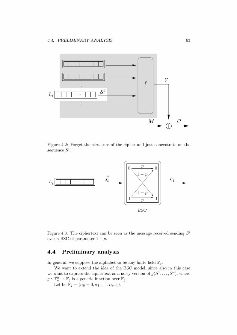
4.4. PRELIMINARY ANALYSIS 63
Figure 4.2: Forget the structure of the cipher and just concentrate on thesequence Si.
Figure 4.3: The ciphertext can be seen as the message received sending Si
over a BSC of parameter 1− p.
4.4 Preliminary analysis
In general, we suppose the alphabet to be any finite field Fq.We want to extend the idea of the BSC model, since also in this case
we want to express the ciphertext as a noisy version of g(S1, . . . , Sn), whereg : Fnq → Fq is a generic function over Fq.
Let be Fq = α0 = 0, α1, . . . , αq−1.

64 CHAPTER 4. RECONSTRUCTION OF STREAM CIPHERS
The BSC of parameter 1 − p can be equivalently defined as a channelwhich in every instant adds 0 to the transmitted bit with probability p oradds 1 to it with probability 1− p.
Therefore, the natural way to extend the BSC model to Fq is to considera channel which in every instant adds αk to the transmitted digit withprobability pk, where k varies in 0, . . . , q − 1 and
∑q−1k=0 pk = 1.
As already specified, we assume the plaintextM = mtt∈N to be nonuni-formly distributed, namely we define
pm,k = P (mt = αk) for all k ∈ 0, . . . , q − 1
where obviously∑q−1
k=0 pm,k = 1, and we suppose there exists at least oneindex k such that pm,k 6= 1
q .
Let gt be the sequence obtained as g(s1t , . . . , s
nt ), while yt = f(s1
t , . . . , snt )
as usual denoted the keystream.Now, let E = εtt∈N be the noise sequence, so that we write gt+ εt = ct
for all t.The noise is distributed as follows:
pk = P (εt = αk) = P (ct − gt = αk) = P (yt +mt − gt = αk) =
=
q−1∑h=0
pm,hP (yt − gt = αk − αh)
We are thus imagining to send the message sequence S = g(S1, . . . , Sn)over a memoryless channel affected by the noise E, which correctly transmita digit with probability p0 or modifies it by one of the constant values αk(k 6= 0), each with probability pk.
The reason why we are interested in any function g of the output of theregisters is given by the theorems we have showed in Chapter 2.
In fact, let P1(x), . . . , Pn(x), Q(x) ∈ Fq[x] be primitive polynomials, then
• if P | Q, then S(P ) ⊆ S(Q) (Theorem 2.11)
• S(P1) + · · · + S(Pn) = S(Q), where Q = lcm(P1, . . . , Pn) and sodeg(Q) =
∑ni=1 deg(Pi) (Theorem 2.12)
• S(P1) · · · S(Pn) = S(Q) where Q is a polynomial such that deg(Q) =∏ni=1 deg(Pi) (Theorem 2.13)
These results explicitly show some relations between the characteristicpolynomial of any sequence obtained as a function of the sequences producedby the registers and the characteristic polynomials of the registers.
In particular, let g be any linear combination, namely g(x) = u ·x, wherex = (x1, . . . , xn) is the unknown vector and u = (u1, . . . , un) is a vector inFnq .

4.4. PRELIMINARY ANALYSIS 65
As we have already seen, the set S(P ) is closed under multiplication fora constant c ∈ Fq, so S and cS are generated by the same polynomial forevery sequence S.
Hence, the sets S(P ) and cS(P ) coincide, implying that the sequenceS = g(S1, . . . , Sn) = u1S
1 + · · ·+unSn is generated by Q = lcm(P1, . . . , Pn)
(Theorem 2.12) or by one of its multiples (Theorem 2.11).
At the same time, according to Remark 2.6, Theorems 2.12 and 2.13assure that if g isn’t linear the sequence S is generated by a polynomial ofdegree much higher than that of lcm(P1, . . . , Pn).
The idea of the reconstruction is thus not to look directly for the poly-nomials Pi, but just for any polynomial Q such that there exists at least onesequence S ∈ S(Q) correlated with the ciphertext.
Such a sequence, in fact, can be seen as a function g of those generatedby (at least someone of) the registers.
If deg(Q) is very high compared to the expected degrees of the feedbackpolynomials, we don’t have any information on the ANF of the function g.
But if Q belongs to a set Ω of polynomials of limited degree, g must bea linear function and we know Q to be a multiple of the polynomials of theregisters involved in the linear combination.
Hence we choose a set Ω whose elements are polynomials whose degreeis bounded by an integer D and mount on it a brute force attack. To reducethe complexity of the attack, we reduce the cardinality of Ω imposing thatits elements must have only a small number d of non-zero coefficients.
We select any polynomial Q ∈ Ω such that there exists a sequence S ∈S(Q) which is correlated with the ciphertext and we factorize everyone ofthe selected polynomials and look for common factors, expect them to bethe polynomials Pi.
The complexity is much reduced compared with a traditional brute forceattempt and the knowledge of the plaintext and the combining function isnot necessary, thanks to the information theory model we use.
In particular, we save much computational complexity thanks to theapproach used to verify the presence in S(Q) of sequences correlated withthe ciphertext.
A trivial way would be trying every possible inizialization to generateevery possible sequence in S(Q), then for each of them test its correlationwith C.
The algorithm proposed by Filiol, instead, allows somehow to check everysequence at the same time, simply rearranging the method used to testcorrelation in Siegenthaler’s attack, and we will do the same.
The idea is to check the correlation between the ciphertext and the mostcorrelated sequence in S(Q). Clearly, we do not know which one it is, butwe will show that this information is not necessary.

66 CHAPTER 4. RECONSTRUCTION OF STREAM CIPHERS
4.5 Reconstruction over FqFirst of all, we need to formalize what we have noticed in the previoussection.
Proposition 4.1. Let S be a generic sequence over Fq and let x = (x1, . . . , xn)denote a vector in Fnq .
If there exists α ∈ Fq such that P (ct − st = α) 6= 1q , then S can be
written as a function of the outputs S1, . . . , Sn of the registers.Namely, there exists a function g : Fnq → Fq such that for all t ∈ N
st = g(s1t , . . . , s
nt )
Moreover, we can write
P (ct − st = α) =
q−1∑k=0
pm,kP (f(x)− g(x) = α− αk)
Proof. Clearly we have
P (ct − st = α) = P (yt +mt − st = α) = P (yt = st + α−mt)
=
q−1∑k=0
pm,kP (yt = st + α− αk)
Now, since α is fixed, if P (yt = st+α−αk) = 1q for all k ∈ 0, . . . , q−1,
we have
P (ct − st = α) =
q−1∑k=0
pm,k1
q=
1
q
q−1∑k=0
pm,k =1
q
which contradicts our hypothesis.Then there must exist at least one k ∈ 0, . . . , q − 1 such that P (yt =
st + α− αk) 6= 1q .
Since in the last equation α−αk is a constant, it means that st and yt arenot statistically independent. Since yt = f(s1
t , . . . , snt ), it means that st isn’t
statistically independent of s1t , . . . , s
nt . Hence, there must exist a function g
such that st = g(s1t , . . . , s
nt ).
Now trivially we can write
P (ct − st = α) =
q−1∑k=0
pm,kP (yt = st + α− αk)
=
q−1∑k=0
pm,kP (f(s1t , . . . , s
nt ) = g(s1
t , . . . , snt ) + α− αk)
=
q−1∑k=0
pm,kP (f(x)− g(x) = α− αk)

4.5. RECONSTRUCTION OVER FQ 67
Remark 4.1. The function g can be explicitly calculated. If we denote st =(s1t , . . . , s
nt ) ∈ Fnq the input vector of f at time t, we can introduce the sets
Tx = t : st = x for all x ∈ Fnq
of all times when x is the input of f .For every Tx we define its subsets
T kx = t ∈ Tx : yt − st = αk for all k ∈ 0, . . . , q − 1
of the times when the difference between the sequences Y and S is αk.These subsets are a partition of Tx, since clearly
q−1⋃k=0
T kx = Tx and T kx ∩ T k′
x = ∅ for all k 6= k′
By Proposition 4.1 we know that the sequences Y and S are not statis-tically independent, so it’s impossible to have
|T kx | =|Tx|q
for all k ∈ 0, . . . , q − 1
Therefore, we can just settle g(x) = αk′ where k′ is such that |T k′x | ≥ |T kx |for all k 6= k′ (if there are more than one index with this property we justchoose one of them).
It’s easy to check that the so defined function g has the properties re-quired by Proposition 4.1.
Note that some of the variables may not appear in the algebraic normalform of g.
For our purpose, the most interesting case is when the function f isτ − correlated for some integer 1 ≤ τ ≤ n, namely when, if we fix the valuesof τ variables, its distribuition changes.
In fact, if there exists a set of indices i1, . . . , iτ ∈ 1, . . . , n, τ elementsui1 , . . . , uiτ ∈ Fq and α ∈ Fq such that
P (f(s1, . . . , sn) = ui1si1 + · · ·+ uiτ s
iτ + α) 6= 1
q(4.5.1)
we can write the 4.5.1 as
P (f(s1, . . . , sn) = g(s1, . . . , sn) + α) 6= 1
q
where g is the linear function g(x) = u · x with u ∈ Fnq and uj = 0 for allj /∈ i1, . . . , 1τ.
It means, as we noticed above, that the sequence S = ui1Si1+· · ·+uiτSiτ ,
generated by the polynomial Q = lcm(Pi1 , . . . , Piτ ), is correlated with the

68 CHAPTER 4. RECONSTRUCTION OF STREAM CIPHERS
ciphertext C, namely the distribution of the sequence C − S isn’t uniform.In particular we could find an imbalance of the sequence C− S on the valueα.
Now, we just need to develop a correlation attack able to detect if apolynomial Q can generate such a sequence.
We then apply the attack to polynomials of limited degree and we obtaina selection of multiples of the polynomials of the registers.
4.5.1 Reconstruction of the registers
Let’s fix two integers d and D and take the set Ω ⊂ Fq[x] defined as
Ω = Q ∈ Fq[x] : W (Q) = d, deg(Q) ≤ D and a0 = 1
where W (Q) denotes the weight of Q, namely the number of non-zero co-efficients of its ANF, and a0 is the free term. We impose a0 = 1 since anyfeedback polynomial has free term 1 according to Definition 2.6.
The generic polynomial we are going to test is then
Q(x) = 1 +d−1∑j=1
ajxij
where aj ∈ Fq for all j ∈ 1, . . . , d−1. It corresponds to the linear feedbackrelation over Fq given by
st =d−1∑j=1
ajst−ij
To understand if S(Q) contains sequences correlated to the ciphertextC, we use the parity check equation defined by Q.
Let S ∈ S(Q) be the sequence with maximal correlation with the cipher-text C.
S can be defined as the sequence in S(Q) maximizing∣∣∣∣∣∣∣∣(P (ct − st = 0), . . . , P (ct − st = αq−1))−(
1
q, . . . ,
1
q
)∣∣∣∣∣∣∣∣namely the sequence such that the distribution of ct− st is the farther fromthe uniform one, with respect to the usual distance defined by the euclideannorm ||·|| in Rq.
Imagining C to be a noisy version of S, we can write ct = st + εt for allt, where the noise sequence E = εt has distribution
pε,k = P (εt = αk) = P (ct − st = αk) for all k ∈ 0, . . . , q − 1
with∑q−1
k=0 pε,k = 1.
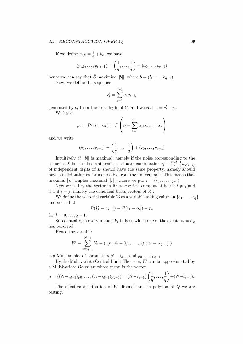
4.5. RECONSTRUCTION OVER FQ 69
If we define pε,k = 1q + bk, we have
(pε,0, . . . , pε,q−1) =
(1
q, . . . ,
1
q
)+ (b0, . . . , bq−1)
hence we can say that S maximize ||b||, where b = (b0, . . . , bq−1).Now, we define the sequence
c′t =
d−1∑j=1
ajct−ij
generated by Q from the first digits of C, and we call zt = c′t − ct.We have
pk = P (zt = αk) = P
εt − d−1∑j=1
ajεt−ij = αk
and we write
(p0, . . . , pq−1) =
(1
q, . . . ,
1
q
)+ (r0, . . . , rq−1)
Intuitively, if ||b|| is maximal, namely if the noise corresponding to thesequence S is the “less uniform”, the linear combination εt −
∑d−1j=1 ajεt−ij
of independent digits of E should have the same property, namely shouldhave a distribution as far as possible from the uniform one. This means thatmaximal ||b|| implies maximal ||r||, where we put r = (r0, . . . , rq−1)
Now we call ej the vector in Rq whose i-th component is 0 if i 6= j andis 1 if i = j, namely the canonical bases vectors of Rq.
We define the vectorial variable Vt as a variable taking values in e1, . . . , eqand such that
P (Vt = ek+1) = P (zt = αk) = pk
for k = 0, . . . , q − 1.Substantially, in every instant Vt tells us which one of the events zt = αk
has occurred.Hence the variable
W =N−1∑t=id−1
Vt = (|t : zt = 0|, . . . , |t : zt = αq−1|)
is a Multinomial of parameters N − id−1 and p0, . . . , pq−1.By the Multivariate Central Limit Theorem, W can be approximated by
a Multivariate Gaussian whose mean is the vector
µ = ((N−id−1)p0, . . . , (N−id−1)pq−1) = (N−id−1)
(1
q, . . . ,
1
q
)+(N−id−1)r
The effective distribution of W dipends on the polynomial Q we aretesting:

70 CHAPTER 4. RECONSTRUCTION OF STREAM CIPHERS
• If every sequence in S(Q) is independent from C, then also S is in-dependent from C and hence ||b|| = 0. This implies that ||r|| = 0too, hence W is a Multivariate Gaussian with mean µ0 = (N −id−1)
(1q , . . . ,
1q
).
We call this hypothesis H0.
• If there exists at least one sequence in S(Q) correlated with C, then||b|| takes the maximal possible value for a sequence in S(Q) and con-sequently the same remark holds for ||r||. W is then a MultivariateGaussian with mean µ = µ0 + (N − id−1)r, where r 6= (0, . . . , 0).
We call this hypothesis H1.
The Gaussian of hypothesis H1 is thus a Gaussian whose mean is a pointon the q-dimensional sphere of ray (N − id−1)||r|| centered in µ0.
The test consist of fixing a ray R and for any Q ∈ Ω compute the vectorW according to its definition. Then we compute ||W − µ0|| and say that
H0 is true if ||W − µ0|| < R
H1 is true if ||W − µ0|| > R
In the first case we discard Q, otherwise we store it.The probability of a “false alarm”, namely to select a wrong polynomial,
is the volume under the Gaussian bell centered in µ0 outside the sphere ofray R and centered in µ0. The probability of a “non detection”, namely todiscard a good polynomial, is the volume under the Gaussian bell centeredin µ inside the same sphere.
To precisely compute these probabilities and to decide how to chosethe ray R we can proceed as done by Filiol on F2 (see the next chapterfor a detailed description). Substantially, we standardize the two variablesreporting both to the Standard MultiNormal whose distribution function isnumerically computable.which generated at least one sequence such that thecorresponding variable W has mean that move away from µ0 of at least adistance (N − id−1)||r||.

4.6. RECONSTRUCTION OVER F2 71
4.6 Reconstruction over F2
In this section we see what happens when q = 2, reporting the work by EricFiliol which inspired this thesis.
As the reader can easily see, the following algorithm is substantially aspecial case of the algorithm seen in section 4.5. Working over F2 permitsto better manage with probabilities and distributions, getting some moreexplicit results. Furthermore, thanks to the properties of the Hammingdistance and consequently to those of the Walsh spectrum of a booleanfunction, the recovery of the combining function can be easily achieved justexploiting some results of the reconstruction of the register.
4.6.1 Introductory results
First of all, we recall that in the binary case we assume the plaintext M =mtt∈N to have distribution
P (mt = 0) = p0, P (mt = 1) = 1− p0 with 0.6 ≤ p0 ≤ 0.7
The following proposition is equivalent to proposition 4.1, but on F2.
Proposition 4.2. Let S = stt∈N be any binary sequence and let x =(x1, . . . , xn) denote a vector in Fn2 .
If P (ct = st) 6= 12 , then S can be written as a function of the outputs
S1, . . . , Sn of the registers.
Namely, there exist a boolean function g : Fn2 → F2 such that for allt ∈ N it holds
st = g(s1t , . . . , s
2t )
Moreover, we can write
P (ct = st) = 1− p0 − pg + 2p0pg
where pg = P (f = g).
Proof. Clearly, it holds
P (ct = st) = P (yt ⊕mt = st)
= P (mt = 0)P (yt = st) + P (mt = 1)P (yt 6= st)
= p0P (yt = st) + (1− p0)(1− P (yt = st))
= 1− p0 − P (yt = st) + 2p0P (yt = st)
Now, P (yt = st) = 12 would imply
P (ct = st) = 1− p0 −1
2+ p0 =
1
2

72 CHAPTER 4. RECONSTRUCTION OF STREAM CIPHERS
which contradicts our hypothesis.Hence P (yt = st) 6= 1
2 , namely st and yt are not statistically independent.Since yt = f(s1
t , . . . , snt ), st is not statistically independent from s1
t , . . . , snt ,
so there must exist a function g such that st = g(s1t , . . . , s
nt ).
Now trivially P (yt = st) = P (f = g) = pg and we can write
P (ct = st) = 1− p0 − P (yt = st) + 2p0P (yt = st) = 1− p0 − pg + 2p0pg
Remark 4.2. Over F2, the recovery of the function g of proposition 4.2 iseven easier. If we denote st = (s1
t , . . . , snt ) ∈ Fn2 the input vector of f at time
t, we can introduce the sets
Tx = t : st = x for all x ∈ Fn2of all times when x is the input of f .
For every Tx, we define its subsets
T 0x = t ∈ Tx : st = yt and T 1
x = t ∈ Tx : st = yt + 1
to distinguish when st = yt or st 6= yt.These subsets are a partition of Tx, since clearly
T 0x ∪ T 1
x = Tx and T 0x ∩ T 1
x = ∅
By proposition 4.2, we know that the sequences S and Y are not statis-tically independent, so it’s not possible to have
|T 0x | = |T 1
x | =|Tx|
2
thus we can settle g(x) = 0 if |T 0x | ≥ |T 1
x | and g(x) = 1 otherwise.It’s easy to check that the so defined function g has the properties re-
quired by proposition 4.2.Note that some of the variables may not appear in the algebraic normal
form of g.
If the function f is τ − correlated, its distribution changes as soon as wefix the values of τ variables. We can exploit this property as follows.
Suppose there exist a set of indices i1, . . . , iτ ∈ 1, . . . , n such that
P (f(s1, . . . , sn) = si1 + · · ·+ siτ ) 6= 1
2(4.6.1)
we can write the 4.6.1 as
P (f(s1, . . . , sn) = g(s1, . . . , sn)) 6= 1
2
where g is the linear function g(x) = u · x with u = (u1, . . . , un) ∈ Fn2 anduj = 1 if and only if j ∈ i1, . . . , 1τ.
Hence the correlation between the ciphertext C and the sequence S =Si1 + · · ·+ Siτ provides informations about the polynomials Pi1 , . . . , Piτ :

4.6. RECONSTRUCTION OVER F2 73
• by theorem 2.12, in fact, S ∈ S(Q), where Q = lcm(Pi1 , . . . , Piτ )
• by theorem 2.11, any polynomial generating the sequence S its Q orone of its multiples
4.6.2 Reconstruction of the registers
To reconstruct the registers, first we fix two integers d and D and take theset Ω ⊂ F2[X] defined as
Ω = Q ∈ F2[X] : W (Q) = d, deg(Q) ≤ D and a0 = 1
where W (Q) denotes the weight of Q, namely the number of non-zero coef-ficients of its ANF, and a0 is the free term.
The generic polynomial we’re going to test is thus
Q(X) = 1 +d−1∑j=1
Xij
which corresponds to the linear feedback relation over F2 given by
st =
d−1⊕j=1
st−ij
To understand if S(Q) contains any sequence correlated to the ciphertextC, we use the parity check equation defined by Q.
We define the sequence
c′t =d−1⊕j=1
ct−ij
which is the one Q would have generated if applied as feedback polynomialto a register with initial state (c0, . . . , cid−i).
For all t ∈ id−1, . . . , N − 1 let
zt = ct ⊕ c′t
be the sequence which in every instant checks if ct = c′t.If we define p := P (ct 6= c′t) = P (zt = 1), for all t the variable zt is a
Bernoulli of parameter p, zt ∼ B(p).To evaluate the correlation between ct and c′t, we compute Z ′ =
∑N−1t=id−1
zt,
which just counts how many times ct 6= c′t.The variables zt being independent and identically distributed, for large
values ofN−id−1, by the Central Limit Theorem, Z ′ can be approximated bya Gaussian with mean µ′ = (N−id−1)p and variance σ′2 = (N−id−1)p(1−p).
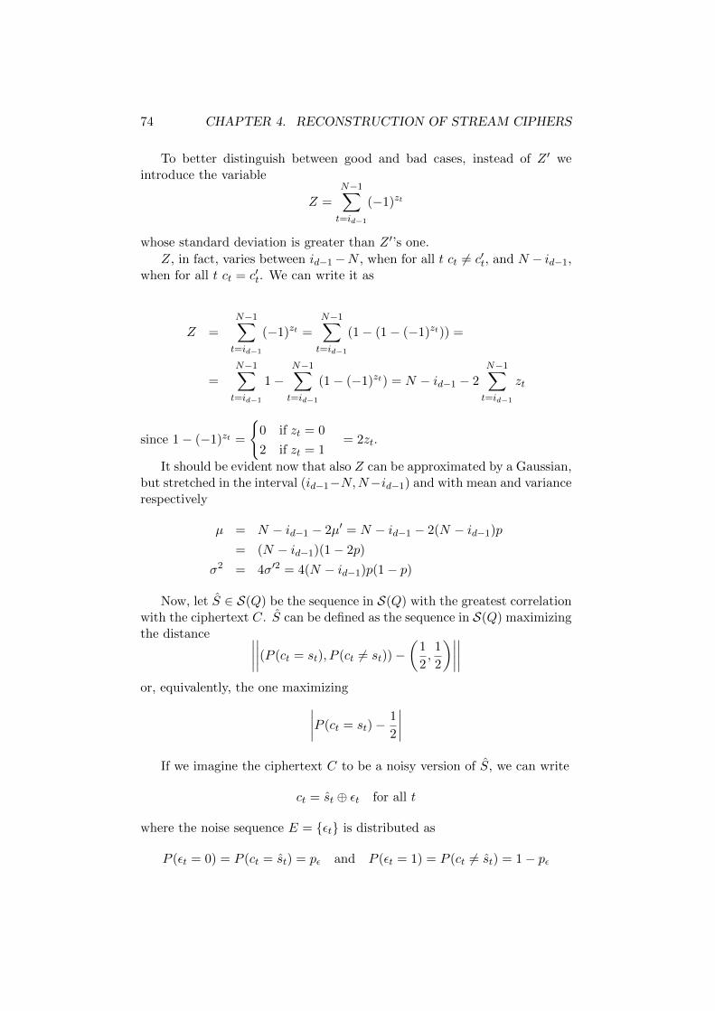
74 CHAPTER 4. RECONSTRUCTION OF STREAM CIPHERS
To better distinguish between good and bad cases, instead of Z ′ weintroduce the variable
Z =N−1∑t=id−1
(−1)zt
whose standard deviation is greater than Z ′’s one.
Z, in fact, varies between id−1−N , when for all t ct 6= c′t, and N − id−1,when for all t ct = c′t. We can write it as
Z =
N−1∑t=id−1
(−1)zt =
N−1∑t=id−1
(1− (1− (−1)zt)) =
=N−1∑t=id−1
1−N−1∑t=id−1
(1− (−1)zt) = N − id−1 − 2N−1∑t=id−1
zt
since 1− (−1)zt =
0 if zt = 0
2 if zt = 1= 2zt.
It should be evident now that also Z can be approximated by a Gaussian,but stretched in the interval (id−1−N,N−id−1) and with mean and variancerespectively
µ = N − id−1 − 2µ′ = N − id−1 − 2(N − id−1)p
= (N − id−1)(1− 2p)
σ2 = 4σ′2 = 4(N − id−1)p(1− p)
Now, let S ∈ S(Q) be the sequence in S(Q) with the greatest correlationwith the ciphertext C. S can be defined as the sequence in S(Q) maximizingthe distance ∣∣∣∣∣∣∣∣(P (ct = st), P (ct 6= st))−
(1
2,1
2
)∣∣∣∣∣∣∣∣or, equivalently, the one maximizing∣∣∣∣P (ct = st)−
1
2
∣∣∣∣If we imagine the ciphertext C to be a noisy version of S, we can write
ct = st ⊕ εt for all t
where the noise sequence E = εt is distributed as
P (εt = 0) = P (ct = st) = pε and P (εt = 1) = P (ct 6= st) = 1− pε

4.6. RECONSTRUCTION OVER F2 75
The condition ct 6= c′t can now be written as
ct 6=d−1⊕j=1
ct−ij
⇔ st ⊕ εt 6=d−1⊕j=1
(st−ij ⊕ εt−ij )
⇔ st ⊕ εt 6=d−1⊕j=1
st−ij ⊕d−1⊕j=1
εt−ij
⇔ εt 6=d−1⊕j=1
εt−ij
since S ∈ S(Q) implies st =⊕d−1
j=1 st−ij .
Furthermore, it holds
p = P (zt = 1) = P (ct 6= c′t) = P
εt 6= d−1⊕j=1
εt−ij
The last condition is true if and only if the number of indices t ∈ t, t−

76 CHAPTER 4. RECONSTRUCTION OF STREAM CIPHERS
i1, . . . , t− id−1 such that εt = 1 is odd, so p can be computed as
p = P
εt 6= d−1⊕j=1
εt−ij
=
d∑l=0l odd
(d
l
)(1− pε)lpd−lε
=1
2
2
d∑l=0l odd
(d
l
)(1− pε)lpd−lε +
d∑l=0
l even
(d
l
)(1− pε)lpd−lε +
−d∑l=0
l even
(d
l
)(1− pε)lpd−lε
(1)=
1
2
d∑l=0l odd
(d
l
)(1− pε)lpd−lε −
d∑l=0l odd
(d
l
)(pε − 1)lpd−lε +
+d∑l=0
l even
(d
l
)(1− pε)lpd−lε −
d∑l=0
l even
(d
l
)(pε − 1)lpd−lε
=
1
2
[d∑l=0
(d
l
)(1− pε)lpd−lε −
d∑l=0
(d
l
)(pε − 1)lpd−lε
](2)=
1
2[1− (2pε − 1)d]
where in (1) we have used
(1− pε)l =
−(pε − 1)l when l is odd(pε − 1)l when l is even
while in (2) we have used Newton’s binomial theorem:
d∑l=0
(d
l
)xlyd−l = (x+ y)d
.
We have therefore defined a variable Z which depends on the polynomialQ we’re testing. Its distribution varies according as Q is correlated with Cor not, since:
1. If every sequence in S(Q) is independent from C, then neither S iscorrelated with C and pε = 1
2 . In this case we can easily check that

4.6. RECONSTRUCTION OVER F2 77
also p = 12(1 − (21
2 − 1)d) = 12 and then Z is a Gaussian with mean
and variance respectively
µ0 = (N − id−1)
(1− 2
1
2
)= 0
σ20 = 4(N − id−1)
1
2
(1− 1
2
)= N − id−1
We call this hypothesis H0.
2. If there exists at least one sequence in S(Q) correlated with the ci-phertext C, then, by definition of S, pε 6= 1
2 , or better the distanceδ = |pε − 1
2 | is the biggest possible one. In this case
p =1
2
[1−
(2
(1
2± δ)− 1
)d]=
1
2(1− (±2δ)d)
where the sign before δ is unknown depending on the sign of pε − 12 .
As we have seen, Z has mean and variance given respectively by
µ = (N − id−1)
(1− 2
(1
2(1− (±2δ)d)
))= (N − id−1)(±2δ)d
σ2 = 4(N − id−1)1
2(1− (±2δ)d)
1
2(1 + (±2δ)d) = (N − id−1)(1− (2δ)2d)
We call this hypothesis H1.
In figure 4.4, we show the two Gaussian bells corresponding to the twohypothesis. As you can see, the situation changes symmetrically accordingas pε >
12 , so that µ > 0, or pε <
12 , so that µ < 0.
Figure 4.4: The Gaussian bell of hypothesis H1 (red) compared with theone of hypothesis H0 (blue) in the two cases.
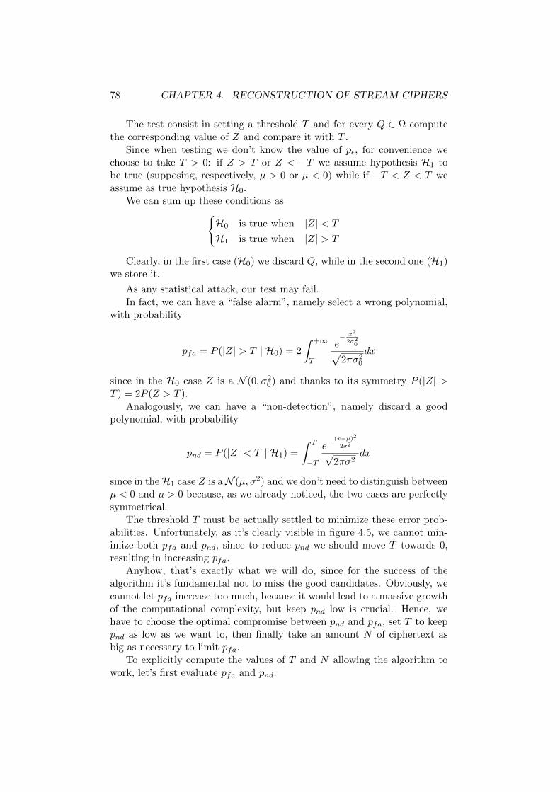
78 CHAPTER 4. RECONSTRUCTION OF STREAM CIPHERS
The test consist in setting a threshold T and for every Q ∈ Ω computethe corresponding value of Z and compare it with T .
Since when testing we don’t know the value of pε, for convenience wechoose to take T > 0: if Z > T or Z < −T we assume hypothesis H1 tobe true (supposing, respectively, µ > 0 or µ < 0) while if −T < Z < T weassume as true hypothesis H0.
We can sum up these conditions asH0 is true when |Z| < T
H1 is true when |Z| > T
Clearly, in the first case (H0) we discard Q, while in the second one (H1)we store it.
As any statistical attack, our test may fail.In fact, we can have a “false alarm”, namely select a wrong polynomial,
with probability
pfa = P (|Z| > T | H0) = 2
∫ +∞
T
e− x2
2σ20√2πσ2
0
dx
since in the H0 case Z is a N (0, σ20) and thanks to its symmetry P (|Z| >
T ) = 2P (Z > T ).Analogously, we can have a “non-detection”, namely discard a good
polynomial, with probability
pnd = P (|Z| < T | H1) =
∫ T
−T
e−(x−µ)2
2σ2
√2πσ2
dx
since in theH1 case Z is aN (µ, σ2) and we don’t need to distinguish betweenµ < 0 and µ > 0 because, as we already noticed, the two cases are perfectlysymmetrical.
The threshold T must be actually settled to minimize these error prob-abilities. Unfortunately, as it’s clearly visible in figure 4.5, we cannot min-imize both pfa and pnd, since to reduce pnd we should move T towards 0,resulting in increasing pfa.
Anyhow, that’s exactly what we will do, since for the success of thealgorithm it’s fundamental not to miss the good candidates. Obviously, wecannot let pfa increase too much, because it would lead to a massive growthof the computational complexity, but keep pnd low is crucial. Hence, wehave to choose the optimal compromise between pnd and pfa, set T to keeppnd as low as we want to, then finally take an amount N of ciphertext asbig as necessary to limit pfa.
To explicitly compute the values of T and N allowing the algorithm towork, let’s first evaluate pfa and pnd.

4.6. RECONSTRUCTION OVER F2 79
Figure 4.5: The area in red is pfa, while the area in blue is pnd.
Let
Φ(x) =
∫ x
−∞
e−y2
2
√2πdy
be the distribution function of the standard normal.
If we standardize the variable, substituting y = xσ0
for hypothesis H0
and y = x−µσ for H1, we obtain
pfa = 2
∫ +∞
Tσ0
e−y2
2
√2πdy = 2
∫ − Tσ0
−∞
e−y2
2
√2πdy = 2Φ
(− Tσ0
)(4.6.2)

80 CHAPTER 4. RECONSTRUCTION OF STREAM CIPHERS
and
pnd =
∫ T−µσ
−T−µσ
e−y2
2
√2πdy = Φ
(T − |µ|σ
)− Φ
(−T − |µ|
σ
)≈ Φ
(T − |µ|σ
)(4.6.3)
since we don’t know if µ > 0 or µ < 0 and in both cases Φ(−T−|µ|
σ
)is
negligible, being << Φ(T−|µ|σ
).
Now we can fix the accepted values for pnd and pfa and invert equations4.6.2 and 4.6.3 (substituting the computed values of σ0, µ and σ) using aStandard Normal Table, obtaining the system
N − id−1 =
(−T
Φ−1(pfa2
))2
T = Φ−1(pnd)√
(N − id−1)(1− (2δ)2d) + (N − id−1)(2δ)d
Solving the system in the unknowns T and N permits to settle the bestvalues for the parameters necessary for the algorithm.
Usually N is given (it’s simply the total amount of available ciphertext),so the second equation is used to settle T , while the first one only allows tocheck if we have enough ciphertext digits to reduce pfa as desired.
4.6.3 The algorithm
We can now expose the algorithm for the recovery of the feedback polyno-mials.
Since δ was defined somehow to measure the “distance” in the distribu-tion of Z between hypothesis H0 and H1, we can fix a minimum acceptedvalue δmin. The following algorithm then examines all polynomials of degreeat most D and of weight d, detecting every polynomial Q in this set suchthat |P (ct 6= c′t)− 1
2)| ≥ δmin.
Algorithm 4.1 (Reconstruction of the registers over F2).
Require: N and ciphertext C = c0c1 . . . cN−1
Choose: a value pnd for the probability to miss a good candidateChoose: a value pfa for the probability to select a wrong a polynomialChoose: a minimum value δminChoose: two parameters d and Dfor each (d − 1)-tuple (i1, . . . , id−1) such that 0 < i1 < · · · < id−1 ≤ DdoN ′ ← N − id−1
T ← Φ−1(pnd)√N ′(1− (2δmin)2d) +N ′(2δmin)d
Z ← 0

4.6. RECONSTRUCTION OVER F2 81
for t = id−1, . . . , N − 1 doc′t =
∑d−1j=1 ct−ij
if ct = c′t thenZ ← Z + 1
elseZ ← Z − 1
end ifend forif |Z| ≥ T then
factorize Q(X) = 1 +∑d−1
j=1 Xij and store the factors
end ifend for
4.6.4 Recovery of the combining function
Once we have implemented algorithm 4.2, the complete recovery of the co-efficients of the combining function can be easily achieved.
First, the reconstruction of the registers tells us the value of n, namelythe number of variables of the combining function f .
Now, any polynomial we have detected is a multiple of some feedbackpolynomials of the registers, thus it’s of the form
Q = R ·∏i∈I
Pi, I ⊆ 1, . . . , n
where R is another polynomial in F2[X].Take any set of indices I and suppose we have collected nI multiples of∏
i∈I Pi, denoted Qj for j = 1, . . . , nI .For any Qj we have computed and stored the corresponding value Zj of
the variable Z. The arithmetic mean of those values gives us an esteem ofthe expected value of Z:∑nI
j=1 Zj
nI≈ E(Z) = N(2pε − 1)d
where pε = P (ct = st) with st = g(s1t , . . . , s
nt ) and g(x) = 1I · x1.
We can thus esteem the value of pε and use it to esteem the value ofpg = p(f = g), since by proposition 4.2 we know that
pε = 1− p0 − pg + 2p0pg
where p0 = P (mt = 0).Finally, from identity 2.2.7, we have
pg =1
2
(1 +
χf (1I)
2n
)11I is the vector in Fn2 whose i-th component is 1 if and only if i ∈ I

82 CHAPTER 4. RECONSTRUCTION OF STREAM CIPHERS
and we can quite precisely esteem the value of χf (1I) since the Walsh coef-ficients of a balanced boolean function are known to be multiple of 4.
We have thus shown how to completely recover the Walsh spectrum ofthe function f . The coefficients of its ANF can be easily evaluated thanksto proposition 2.11:
au = 2wH(u)−1
1− 1
2n
∑vu
χf (u)
mod 2

Bibliography
[1] Berlekamp, E.R. : Algebraic Coding Theory, McGraw-Hill, New York,1968.
[2] Canteaut, A., and Filiol, E. : Ciphertext Only Reconstruction of StreamCiphers Based on Combination Generators, in: Proceedings of Fast Soft-ware Encryption 2000, ed. by SCHNEIER, B., Lecture Notes in Com-puter Science 1978, Springer Verlag, 2001.
[3] Canteaut, A., and Filiol, E. : Ciphertext Only Reconstruction of LFSR-based Stream Ciphers, Rapport de Recherche INRIA, n 3887, February2000, Institut National de Recherche en Informatique et Automatique,Domaine de Voluceau, B.P. 105, 78153 Le Chesnay cedex.
[4] Diffie, W., and Hellman, M.E. : New Directions in Cryptography, IEEETransactions in Information Theory, Vol. IT-22, Nr. 6, 1976, pp 644-654.
[5] Filiol, E. : Techniques de Reconstruction en Cryptologie et Theorie desCodes, Ph. D Thesis, Ecole Polytechnique, France 2001.
[6] Geffe, P.R. : How to Protect Data with Ciphers that Are Really Hard toBreak, Electronics, pp 99-101, 1973.
[7] Golomb, S.W. : Shift Registers Sequences, Aegean Park Press, 1982.
[8] Herlestam, T. : On the complexity of certain crypto generators, in :Security, IFIP/Sec’83, North Holland, 1983.
[9] Kerckhoffs, O. : La Cryptologie Militaire, Louis BAUDOIN ed., Paris,1883.
[10] Lidl, R., and Niederreiter, H. : Finite Fields, Encyclopedia of Mathe-matics and its Applications, 20, Cambridge University Press, (2008).
[11] Meier, W., and Staffelbach, O. : Fast Correlation Attack on CertainStream Ciphers, Journal of Cryptology, pp 159-176, 1989.
[12] Meier, W., and Staffelbach, O. : Nonlinearity Criteria for Crypto-graphic Functions, in: Advances in Cryptology - EUROCRYPT ’89,
83

84 BIBLIOGRAPHY
Lecture Notes in Computer Science 434, pp 549-562, Springer Verlag,1990.
[13] Rueppel, R.A., and Staffelbach, O. : Products of Linear Recurring Se-quences with Maximum Complexity, IEEE Transactions on InformationTheory, Vol. 33 (1), pp 124-131, 1987.
[14] Shannon, C.E. : A Mathematical Theory of Communication, Bell Sys-tem Journal, Vol. 27, pp 379-423 (Part I) and pp 623-656 (Part II),1948.
[15] Shannon, C.E. : Communication Theory of Secrecy Systems, Bell Sys-tem Technical Journal, Vol. 28, Nr. 4, pp 656-715, 1949.
[16] Siegenthaler, T. : Correlation Immunity of Nonlinear Combining Func-tions for Cryptographic Applications, IEEE Transactions on InformationTheory, Vol. 35, Nr. 5, September 1984, pp 776-780.
[17] Siegenthaler, T. : Decrypting a Class of Stream Ciphers Using Cipher-text Only, IEEE Transactions on Computers, C-34, 1, pp 81-84, 1985.
[18] Van Oorschot, P., Menezes, A., and Vanstone, S. : Handbookof Applied Cryptography, CRC Press, fifth printing edition (2001).http://www.cacr.math.uwaterloo.ca/hac/
[19] Xiao, G.-Z., and Massey, J.L. : A Spectral Characterization ofCorrelation-Immune Combining Functions, IEEE Transactions on In-formation Theory, Vol. IT-34, Nr. 3, pp 569-571, 1988.
[20] http://en.wikipedia.org/