cid working paper no. 133 :: south africa: macroeconomic ... · pdf filesouth africa project...
TRANSCRIPT

South Africa: Macroeconomic Challenges after a Decade of Success
Jeffrey Frankel, Ben Smit, and Federico Sturzenegger
CID Working Paper No. 133 September 2006
© Copyright 2006 Jeffrey Frankel, Ben Smit, Federico Sturzenegger, and the President and Fellows of Harvard College
at Harvard UniversityCenter for International DevelopmentWorking Papers
South Africa project Macroeconomic Challenges after a Decade of Success
2
South Africa: Macroeconomic Challenges after a Decade of Success Jeffrey Frankel1, Ben Smit2, and Federico Sturzenegger1
DRAFT, first version July 2006, this version September 2006 Abstract: The South African economy has been doing well. Capital inflows and the rand have been strong, growth was high in 2005, the budget is relatively healthy, and inflation rates and interest rates are low. As democracy continues to consolidate, there are plenty of grounds for optimism. Is the job done, or do these achievements open the door to new challenges? What are the risks in the horizon? And how does the government’s ASGI-SA strategy deal with the challenges? This report provides four areas of analysis: an analysis of the current account, the consistency of the ASGI-SA program, the benefits of the current fiscal-macro policy mix and the choice of exchange rate regime. We suggest that ASGI-SA relies too heavily on capital accumulation, in a way that other growth accelerations have not. In addition there are grounds for doubt whether the required jump in investment will be forthcoming, and for worry by how much it would deteriorate South Africa's current account deficit. South Africa would suffer less from a sudden stop of capital inflows than would other emerging economies, particularly because most of the inflows do not take the form of debt denominated in foreign currency. Nevertheless, the already-large current account deficit is worrisome. South Africa is still exposed to a possible a sudden stop, particularly one triggered by a reversal of the global climate for mineral commodities and emerging markets generally. We offer some proposals for reducing this vulnerability. They include avoidance of pro-cyclical fiscal policy and active intervention by the monetary authorities to build up reserves and dampen real exchange rate appreciations. Keywords: South Africa, ASGI-SA JEL Codes: 055, E00, E61, E63 1) Kennedy School of Government and Center for International Development, Harvard University 2) Bureau for Economic Research, University of Stellenbosch The authors would like to thank Philippe Aghion for his contribution to Part III and to Federico Dorso and M. Melesse Tashu for very capable research assistance. Ricardo Hausmann provided significant input and Lawrence Harris provided a wonderful discussion in the July meetings with Treasury in Pretoria. Stan du Plessis provided careful and comprehensive comments of an earlier draft. This report has also nurtured from extensive discussion with all the team engaged in the project as well as with talk with government officials and South African academics. We particularly thank Johannes Fedderke, Brian Kahn, Ismael Momoniat, and Theo van Rensburg, for sharing ideas and suggestions for this report. Alan Hirsch also provided guidance as to the main issues that should be covered. Trevor Manuel enlightened us with a careful description of the issues in our January trip to South Africa. This paper is part of the CID South Africa Growth Initiative. This project is an initiative of the National Treasury of the Republic of South Africa within the government’s Accelerated and Shared Growth Initiative (ASGI-SA), which seeks to consolidate the gains of post-transition economic stability and accelerate growth in order to create employment and improve the livelihoods of all South Africans.
South Africa project Macroeconomic Challenges after a Decade of Success
3
INDEX
Page EXECUTIVE SUMMARY
1. Current account vulnerability 2. The consistency of ASGI-SA program 3. The fiscal-monetary policy mix 4. Exchange rate regimes
5 6 6 7
INTRODUCTION 8
PART I. CURRENT MACRO SITUATION: MANAGING A BOOM 11 1. Long term trends 2. Recent dynamics and looking forward
a. Investment b. Consumption c. The Current Account d. A simulation
3. Why is South Africa running a current account deficit when most emerging markets this time around are running surpluses? a. An estimation exchange rate equation for the rand
4. Managing capital outflows in a sudden stop a. Could there be a repeat across all emerging markets, as in 1982, and
1997-98? b. Or have things fundamentally changed?
i. “This time is different” ii. More flexible currencies iii. Higher reserve levels iv. Collective Action Clauses v. Less dollar-denominated debt vi. More openness to FDI and trade vii. So, some things are different this time around
c. Could it happen now? d. How does South Africa compare to others in indicators of
vulnerability? i. Capital inflows going to Current Account deficits instead of
reserves ii. Debt levels iii. Exports/GDP ratio iv. Composition of inflow
1. Currency of denomination 2. Equity component versus borrowing 3. Bank debt vs. Bonds 4. Short term vs. long term
v. Simulations
11 14 15 18 19 20 27
28 31 31
31 31 32 32 32 33 34 35 36 39
39
40 43 47 47 47 48 49 50
PART 2. THE CONSISTENCY OF THE ASGI-SA PROGRAM
54
South Africa project Macroeconomic Challenges after a Decade of Success
4
PART 3. FISCAL AND MONETARY POLICY IN A COMMODITY-BASED ECONOMY
59
1. Inflation targeting and stabilization 2. The fiscal and monetary policy mix in South Africa 3. Thinking about the procyclicality of fiscal policy 4. Options for managing fiscal policy
a. The design of fiscal policy in a commodity-exporting country b. Debt management for reduced vulnerability
i. The composition of inflows and better risk-sharing ii. A proposal to link bonds to mineral commodity prices
59 60 65 69 69 69 70 70
PART 4. ALTERNATIVE WAYS TO MANAGE INFLOWS AND THE EXCHANGE RATE REGIME
1. Allow appreciation a. Has the float allowed the rand to become overvalued? b. Arguments for avoiding overvaluation
i. The Dutch Disease ii. Growth effects iii. Intervention to add to reserves
2. Intervene to dampen appreciation 3. Capital controls
a. Possibility of putting controls on inflows b. Possibility of removing any remaining barriers to outflows
4. Choice of exchange rate regimes
73
73 73 74 74 74 75 76 79 79 80 80
APPENDIX 83
REFERENCES 85

South Africa project Macroeconomic Challenges after a Decade of Success
Macroeconomic Challenges after a
Decade of Success
EXECUTIVE SUMMARY Halfway through the new decade, the South African economy has done very well. Growth was high in 2005, capital inflows and the rand are strong, the budget is relatively healthy, and inflation rates and interest rates are low. As democracy continues to consolidate, there are plenty of grounds for optimism; in fact business confidence indicators and private investment are at an all time high. This report asks the question if such achievements provide grounds for complacency. In other words, is the job done? Or do these achievements open the door to new challenges? Are there risks in the horizon? And how does the government’s ASGI-SA strategy deal with the challenges? This report provides four areas of analysis: an analysis of the current account, the consistency of the ASGI-SA program, the benefits of the current fiscal-macro policy mix and the choice of exchange rate regime. We discuss our main conclusions for each in turn. 1. Current account vulnerability. In contrast to many other emerging economies South Africa’s current expansion has come hand in hand with a large current account deficit, which in the first quarter of 2006 topped 6% of GDP. An optimistic view would hold that the deficit reflects rational adjustment to a new equilibrium of permanently higher commodity prices, high investment, or previously pent-up consumption by a new middle class. A pessimistic view is that the boom is unsustainable, perhaps because of a temporary spike in global mineral prices in 2006, because consumers do not fully understand the restrictions they face, or because there is always the risk of a sudden stop of capital inflows. According to this view it is important to keep imbalances in check and to think about managing the inflows in such a way as to minimize the likelihood and severity of the sort of crisis that afflicted other emerging markets in the 1990s. Even if the terms of trade have not risen spectacularly – the big rise in prices for South African mineral exports having been substantially offset by a big rise in the price of oil imports – we think that the global commodity boom, together with the emerging market boom, is nonetheless largely responsible for the appreciation of the rand. The reason is that investors have piled into South African assets (especially equities), thus bidding up their price, not only in the form of higher rand prices of equities but also in the form of an appreciation of the currency. Easy money emanating from the world’s major central banks (Fed, BoJ, ECB, and PBoC) over the period 2001-2005, together with a possible bubble component over the period 2005-06, have probably been one force
5

South Africa project Macroeconomic Challenges after a Decade of Success
6
behind the movement into commodities generally, emerging markets at large, and commodity-based emerging markets in particular. The real appreciation of the rand is in turn one reason for the country’s large current account deficit. The bad news is that the bubble component may be especially applicable to South Africa because most other emerging markets are running trade surpluses now. The good news is that even if a crash comes – spring 2006 saw a hint of it -- South Africa is well-positioned to weather it for a number of reasons: borrowing has been a relatively small fraction of the inflow (versus equity and FDI), the rand floats (though not without substantial intervention), and much of the debt is rand-denominated. These factors offer good grounds for hope that a correction will be fairly automatic and not involve the painful “currency crash plus balance sheet contraction” so familiar from the emerging market crises suffered by other countries in 1994-2001. While a large crisis is off the books, we provide a series of simulations that suggest that a significant reversal in flows would nevertheless impact the South African economy by slowing growth, hurting investment and, potentially, worsening fiscal accounts. In addition we show that the current growth scenario requires increasing terms of trade just to keep the current account in recent levels,. If the terms of trade were to stabilize – let alone deteriorate -- the current growth dynamics would lead to a significant deterioration of external accounts. Thus, our report can be read as sending a cautionary note on the need to reduce the external imbalances of the economy. We also provide some policy recommendations to further minimize the negative impact of a possible sudden stop. For example with regard to debt management our advice is that South Africa seek further to reduce the share of capital inflow that takes the form of short-term and dollar-denominated debt, by taking advantage of its ability to borrow in rand and to attract equity and FDI inflows. As a more novel proposal, we suggest that, when the South African government undertakes major borrowing, it consider denominating some of the liabilities in terms of gold, platinum, or prices of other major mineral exports, in hopes of getting such a market going. 2. The consistency of ASGI-SA program. To make a statement on the “macro-consistency” of ASGI-SA we start by reviewing successful growth transitions. In particular, Rodrik (1998) shows that successful growth accelerations have the feature that for each 3% percentage points of increase in output growth investment to GDP ratios increased by just 1%. This implies that growth has come much more from productivity improvements than capital deepening. However when analyzing South Africa’s growth program we see these numbers are inverted: a 1% increase in the growth rate requires a 3% increase in the investment to GDP ratio. We show that this is not capricious. Given the employment/productivity performance of the South African economy even such large investment program will barely deliver the desired growth rates while imposing an impossible burden on public investment. All these are important problems even before discussing the feasibility of increasing domestic savings to finance this program without increasing further the external vulnerability of the economy. As a result we believe the program has serious macro inconsistencies that need to be discussed. 3. The fiscal-monetary policy mix. We evaluate the business cycle features of fiscal and monetary policy to find that so far fiscal policy has been mostly procyclical, whereas monetary policy has shown less evidence, over the last couple of years, of the mild countercyclical pattern it had established during the late nineties. In fact we see a central bank increasingly enthusiastic about its successful inflation targeting strategy. We show, however, that when an economy faces important supply shocks inflation targeting exacerbates the business cycle and not the other way

South Africa project Macroeconomic Challenges after a Decade of Success
7
around. Inflation targeting is fine, but any increases in the CPI attributable to increases in dollar prices of imports, or negative supply shocks, should not prompt monetary tightening to prevent prices from rising. For example, the recent sudden stop, by depreciating the Rand, has rekindled inflation fears at the Central Bank prompting it to raise its discount rate. We believe this is not an optimal policy response. We show, by analyzing South Africa’s output response to fiscal and monetary shocks, that monetary policy is the most convenient tool for implementing countercyclical macro policy. We believe the Central Bank has earned the credibility to push in this direction. In contrast fiscal policy should remain “passively” countercyclical -a countercyclicality that should arise from a relatively stable expenditure pattern combined with procyclical tax revenues. We show that such countercyclical fiscal policy provides growth gains.
4. Exchange rate regimes. The exchange rate regime choice is intimately related to the objectives of monetary policy. We recommend that the authorities continue to float, so that they can pursue a countercyclical macro policy, but also continue to manage the float somewhat by intervening to stabilize the exchange rate. In fact we show that cross country evidence suggests that fighting exchange rate appreciation is associated with higher growth in the future. As a result we propose an active exchange rate policy to keep the currency from becoming overvalued. We discuss how this could be done.

South Africa project Macroeconomic Challenges after a Decade of Success
INTRODUCTION
By early 2006 the South African economy was “making history” in the words of local analysts.
The Bureau of Economic Research (BER) second quarter 2006 Economic Prospects pointed out some of the outstanding facts: Real GDP growth had averaged 4.9% in 2005, the fastest growth rate since the (short-lived)
spurt of 1984; the current business cycle upswing was running at a record 19 months old;
Real household consumption expenditure grew by 6.9%, the fastest annual growth rate since 1981;
2004 and 2005 showed the lowest inflation rates recorded in 37 years;
Long-term interest rates registered a 35-year low of 7.3% early in 2005;
The household debt ratio accelerated to a record high 65.6% at the end 2005; yet the household debt service ratio remained close to a 25-year low at 7%;
The budget deficit was estimated at 0.5% of GDP for fiscal 2005/6, i.e. the lowest in 25 years;
The gold price reached a 25-year high early in 2006; and
The financial account of the balance of payments recorded an inflow of Rand 98.4 billion, the largest ever, though, of course, this net capital inflow financed a large current account deficit of Rand 64.4 billion, or 4.2% of GDP. In the first quarter of 2006, the deficit hit 6.4% of GDP, the highest since 1982.
In fact an outsider could have strengthened this list with a few additional but important long
term factors that make the South African economy stronger than the typical emerging market economy: a very developed financial sector, “no original sin,” world class corporations, a central bank with strong credibility, low budget deficits, low public sector debt levels, and a successful political transition towards a democratic government which has been able to improve social policies.
Is this rosy picture sufficient to justify complacency? This report aims to analyze this question. The preceding list already hints at some of the problems, most importantly a burgeoning current account deficit, and its counterpart, significant capital inflows that may have led to an undesirable real exchange rate appreciation. While it can be argued that the real exchange rate is now comfortably within range of its long run PPP value, the economy combines a large current account deficit with a very high unemployment rate, while exports volume performance has been more lackluster over recent years. Thus, it came not necessarily as a surprise that the current account deficit had topped 6% of GDP in the first quarter of 2006.
While the current account deficit may or may not cast doubts on the external sustainability -- it can always be argued that capital inflows will be enough to compensate the disequilibria -- it is
8

South Africa project Macroeconomic Challenges after a Decade of Success
9
clear that under a large investment expansion, as expected in the Accelerated Shard Growth Initiative (ASGI-SA) proposal, external imbalances would be poised to widen further. And then there is the increase in consumer debt ratios, exposing consumers to a sudden increase in interest rates. What do these risks imply for policy decisions?
In addition, questions can be raised about the fiscal-monetary policy mix currently in place. The South African Reserve Bank (SARB) has keenly defended operating under an inflation targeting rule. But in an economy with supply shocks, a strict inflation targeting rule implies that monetary policy becomes procyclical rather than countercyclical. Moreover, this could put additional pressure on fiscal policy to offset business fluctuations. How focused is the SARB on inflation as its sole objective? And to the extent that fiscal policy is in itself constrained by political restrictions, how effective is the current policy mix?
Following these motivations, the report aims to address several specific questions. First we ask about the sustainability of the current trends in the South African economy going forward. What are the drivers of the current boom? Is this a demand driven expansion with little potential for sustainability? Will growth be constrained by external factors? Should we fear a worsening of the fiscal situation going forward that would call for more prudent fiscal policies today? We find that the expansion is driven by a mild consumption boom (mostly durables) and an increase in investment. But the increase in investment has focused on the nontradable sector, thus auguring future imbalances. In fact when we use BER’s and Treasury’s macro model to simulate the future path of the economy, we find that absent an exogenous improvement in the terms of trade, South Africa will show increasing external imbalances.
Given the size of external imbalances we discuss the possibility of a sudden stop of capital inflows, a possibility that has become more topical with the global financial market turmoil of spring 2006, and what implications such a sudden stop would have for the South African economy. Were it to materialize, as in the late nineties, how prepared is the South African economy to deal with it? As of mid-2006, it looks possible that a period of interest rate tightening in the large economies might precipitate a reversal of the booms in commodities and emerging markets that developed over the preceding five years. How vulnerable is the South African economy to a sudden stop of capital inflows? What are the policy implications? We find that the South African economy is much better prepared than other emerging economies, but would still have to undergo a sizable adjustment if a sudden stop does occur: output would stagnate, consumption would fall, and the government accounts would deteriorate. Thus, we recommend a series of actions to decrease this vulnerability.
We then turn to an analysis of the consistency of the ASGI-SA program. The program is fairly comprehensive including proposals in a wide range of areas. But from a macro perspective the main question relates to the fact that ASGI-SA anticipates a sizable increase in public investment. How will this increase in investment be financed? And what is its potential effect on the current account? If, as we will show, the current ASGI-SA framework poses a major challenge in terms of external sustainability, what are the policy options to make the program feasible? And then there is still the question of whether there will be productive opportunities for such a large increase in public infrastructure. Or will the economy just pile up a large number of “white elephant” projects? Here we raise a note of caution. The program as currently envisioned may not be consistent with macroeconomic balance, and envisions a productivity of investment that is roughly nine times smaller than what has been observed in typical growth accelerations. We discuss why, and conclude that this finding emphasizes the need of substantial productivity gains to reduce the pressure on investment as the main driver of the growth process.

South Africa project Macroeconomic Challenges after a Decade of Success
10
We then move to a discussion of the fiscal-monetary policy mix. The current framework has the Central Bank focusing on inflation with macroeconomic stabilization in the hands of fiscal authorities. It could be argued that so far both have been successful, with inflation at historical lows, the budget in balance and the economy booming. But will this be the case in the future once conditions change? To discuss this issue we develop statistical measures of the relative contribution of fiscal and monetary policy to the recent business cycles to evaluate to what extent it is true that the SARB has remained oblivious to the evolution of the business cycle, and how much can fiscal policy actually achieve. We also try to assess what the data have to say about how effective both monetary and fiscal policy have been as stabilization tools. We show that the evidence points to a more effective role of monetary policy as a stabilization tool. And that fiscal policy has been procyclical over the recent past. The discussion will lead naturally to a debate as to whether there are certain fiscal rules that should be followed. We will argue strongly for reducing procyclicality in fiscal policy by assessing its effect on growth.
We then move to the analysis of the exchange rate regime. We first take a flip side approach to our concern about the sudden stop above and discuss policy options when facing sustained capital inflows. What should be done and what can be done? We discuss the effectiveness of alternative intervention policies, reviewing the evidence, and sharing some cross country evidence that suggests that countries that avoid large real appreciations show better growth performance. We then discuss the inflation targeting dilemma and the choice of monetary regime. Some evidence suggests that during the 90s monetary policy has been mostly countercyclical, dispelling doubts that the inflation regime may lead to an excessively procyclical monetary policy. This leads to our recommendation that the SARB should use its hard earned credibility to broaden the scope of its objectives to include the real exchange rate and the business cycle.

South Africa project Macroeconomic Challenges after a Decade of Success
PART I. CURRENT MACRO SITUATION: MANAGING A BOOM
1. Long term trends Any analysis of South Africa’s macro performance needs to start with a historical overview of the long term dynamics of output growth. Figure 1.1 shows how income per capita increased rapidly during the 1960-1980 period, but then experienced a sharp reversal that lasted for the ensuing 15 years. Only since mid 1995 has the economy recovered its upward trend.
These wide swings beg for an explanation. How can an economy experience such a turnaround in its growth performance? Two factors can immediately be adduced: first a significant weakening of the terms of trade in the 1980s and 1990s, relative to the averages enjoyed during the 1975-1980 years (Figure 1.2); second the anticipation of a change of political regime that led to a collapse of private and public investment (Figures 1.3 and Figure 1.4). In fact public investment shows a dramatic collapse, much larger than that of private investment, which in addition recovers in the aftermath of a successful political transition.1
Figure 1.1 Income per capita
8.3
8.4
8.5
8.6
8.7
dese
ason
aliz
edlg
dppe
rcap
ita
1960q1 1965q1 1970q1 1975q1 1980q1 1985q1 1990q1 1995q1 2000q1 2005q1Period in Stata format: 1960q1=0
1 See du Plessis and Smit (2006) for a comprehensive review of recent South Africa growth experience including an analysis of the relative contribution of productivity capital and labor and a review of existing literature. Where not specified, data for our graphs were obtained from the IFS, WEO or official government statistics.
11

South Africa project Macroeconomic Challenges after a Decade of Success
Figure 1.2 Terms of Trade
.81
1.2
1.4
tot
1960q1 1965q1 1970q1 1975q1 1980q1 1985q1 1990q1 1995q1 2000q1 2005q1Period in Stata format: 1960q1=0
Figure 1.3 Private Investment
.06
.08
.1.1
2.1
4in
vpriv
gdp
1960q1 1965q1 1970q1 1975q1 1980q1 1985q1 1990q1 1995q1 2000q1 2005q1Period in Stata format: 1960q1=0
Figure 1.4. Public Investment
12
.04
.06
.08
.1.1
2in
vpub
licse
ctor
gdp
1960q1 1965q1 1970q1 1975q1 1980q1 1985q1 1990q1 1995q1 2000q1 2005q1Period in Stata format: 1960q1=0

South Africa project Macroeconomic Challenges after a Decade of Success
Figure 1.5 Per capita GDP net of TOT
-.3-.2
-.10
.1.2
gdps
into
t
1960q1 1965q1 1970q1 1975q1 1980q1 1985q1 1990q1 1995q1 2000q1 2005q1Period in Stata format: 1960q1=0
Figure 1.6 South Africa and Malaysia
7
7.5
8
8.5
9
9.5
10
1980 1981 1982 1983 1984 1985 1986 1987 1988 1989 1990 1991 1992 1993 1994 1995 1996 1997 1998 1999 2000 2001 2002 2003 2004 2005 2006 2007
Malaysia South Africa
Figure 1.5 undertakes a simple exercise to assess the quantitative relevance of these factors, by netting out from the GDP per capita figures the effect on GDP of terms of trade changes.2 The figure shows that once the effect of terms of trade is netted out the large reversal is somewhat muted, indicating that terms of trade, on their own, help explain some of the decline in South Africa’s GDP in the 1970s and 1980s. Somewhat curiously, the first and last ten years of the
13
2 This is done simply by regressing deseasonalized GDP per capita on terms of trade, and subtracting the estimated effect of this variable. A similar exercise (not shown) could be done if assuming that public investment is exogenous and subtracting the effect of both terms of trade and public investment. The results would be very similar.

South Africa project Macroeconomic Challenges after a Decade of Success
sample are exceptions, with at least some growth in the 1960s and 1990s that appears unrelated to terms of trade changes.
A more comprehensive review of growth dynamics is given in du Plessis and Smit (2006).
It basically concludes that productivity has been the main driver of output growth in the 1990s with relatively minor contributions of labor and capital. Table 1, adapted from their paper shows the results. Arora and Bhundia (2003), in turn, show that machinery investment and trade openness have been important drivers of South Africa’s productivity growth.
Table 1.1 Sources of Growth
Source: du Plessis and Smit (2006).
At any rate, performance since the 1990s has been much better than in the previous decade. Figure 1.6 illustrates the turnaround by showing a comparison with Malaysia, an economy that has been referred to within the context of the project. As can be seen Malaysia manages a significant convergence with South Africa. But this convergence occurs entirely during the 1980s, when the South Africa economy could not cope with a deteriorating external environment, whereas in the nineties growth performance is very similar.
This leads to the question whether today the South African economy is building sufficient flexibility to deal with a more unfriendly external scenario. It is well known that a measure of such flexibility is the exports to GDP ratio which has been found, not only to be related to the possibility of a growth acceleration, but also to the capacity of an economy to respond to an external shock (Guidotti et al, 2004). It has also been shown to reduce the probability of facing a sudden stop in the first place (Cavallo and Frankel, 2005)3. In the case of South Africa, the exports to GDP ratio has increased somewhat from its lows during the 1980-1985 period, but remains at 25%, lower than it could be.
We conclude that even though the economy is growing fast, past history suggests that the
South African economy has little flexibility on the production side to cope with negative real shocks. It is still insufficiently open. 2. Recent dynamics and looking forward
Figure 1.7 starts our discussion of current business dynamics by measuring the business cycle over the last twenty years. This is done through the usual procedure of running a simple HP filter over the deseasonalized GDP series with the deviations from the trend corresponding to the
14
3 Cavallo and Frankel (2006) find that an increase in the trade/GDP ratio of 10 percentage points decreases the likelihood of a sudden stop by 32%!

South Africa project Macroeconomic Challenges after a Decade of Success
business cycle. Data is shown since 1985. Two features stand out from Figure 1.7. First is the increasing stability of output dynamics, with business cycles appearing milder after 1995 than in the prior ten years. Second, the current cycle does not appear unusually strong; in fact, it looks relatively mild compared to previous episodes (see du Plessis and Smit, 2006, for additional indicators).
Figure 1.7 The business cycle
-.04
-.02
0.0
2.0
4
1 9 8 5 q 1 1 9 9 0 q 1 1 9 9 5 q 1 2 0 0 0 q 1 2 0 0 5 q 1P e r io d i n S t a t a f o r m a t : 1 9 6 0 q 1 = 0
H P _ d e s e a s o n a l i z e d l g d p p e r c a p it a _ 1 c e r o
Focusing on the recent expansion Table 1.2 shows the evolution of main macroeconomic aggregates over the recent past. The table underscores several key features of the current expansion. In particular a significant change in regime appears to take place in 2003, with investment picking up significantly, followed by domestic and public consumption, while exports have lagged behind. What can we say about the nature of these increases in investment and consumption?
Table 1.2 Current macro trends
a. Investment
The data show that investment is on the rise, with private investment at a historical peak, though with total investment at less than 18.2% in the first quarter of 2006 it remains significantly lower than that of high-growing economies. To the extent that ASGI-SA will attempt to increase the investment rate of the economy, this provides a measure of the challenges ahead. If investment would have to increase beyond current levels to foster higher growth, is there any reasonable possibility that it can increase substantially above its historical peak?
15

South Africa project Macroeconomic Challenges after a Decade of Success
To understand further current investment trends in Figures 1.9-1.11, we compute several addition splits of total investment (Figure 1.8): into tradables and nontradables (Figure 1.9), into “consumption” and “productive” investment (Figure 1.10) and machinery investment (Figure 1.11).
Figure 1.8 Total Investment
.1.1
5.2
.25
inve
stm
entg
dp
1960q1 1965q1 1970q1 1975q1 1980q1 1985q1 1990q1 1995q1 2000q1 2005q1Period in Stata format: 1960q1=0
Figure 1.9 Investment in Tradables and Nontradables
0.0
5.1
.15
1960 q1 1 965q1 197 0q1 19 75q1 1980 q1 19 85q1 1 990q 1 199 5q1 20 00q1 2005 q1P erio d in S tata fo rmat : 19 60q1 =0
inv tradables inv nontrad ables
Figure 1.10 Productive and Consumption Investment
16

South Africa project Macroeconomic Challenges after a Decade of Success
.02
.04
.06
.08
.1
1960q1 1965q1 1970q1 1975q1 1980q1 1985q1 1990q1 1995q1 2000q1 2005q1Period in Stata format: 1960q1=0
productiveinvestmentgdp consumptioninvestmentgdp
Figure 1.11 Machinery Investment
.02
.04
.06
.08
mac
hine
rygd
p
1960q1 1965q1 1970q1 1975q1 1980q1 1985q1 1990q1 1995q1 2000q1 2005q1Period in Stata format: 1960q1=0
When investment is split into investment in tradables and in nontradables (investment in tradables is defined as investment in the mining and manufacturing sectors). It can be seen that investment in the tradable sector has typically oscillated around 5% of GDP, though in the recent boom it has edged down. In fact the data show that the recent recovery of investment is mostly in nontradables investment.4 The extent that the recent expansion of the South African economy has not been led by exports points to the lack of interesting investment opportunities in the tradable sector as a potential “binding constraint” on the economy.
Finally one last distinction for investment is that between "consumption" investment
(residential building and transportation) and investment for "productive" activities.5 Analysts have
4 This includes investment in electricity, telecommunications, construction, etc. Some of these may be complementary to tradables production so the distinction should be taken with care.
17
5 While transportation equipment used for consumption should be included in durables consumption and not in investment, some is likely to be statistically catalogued within the investment group.

South Africa project Macroeconomic Challenges after a Decade of Success
pointed out that an increase in “consumption” investment could lead to a less sustainable growth path than if the expansion would have taken place in “productive” investment, as the former does not lead to future production increases.6
Although the graph shows that in recent years "consumption" investment has risen
somewhat more strongly, it is still less than half of productive investment which experienced a significant and sustained recovery in the early nineties. In order to avoid any discussion on methodological issues, figure 1.11 shows the evolution of machinery investment, which shows an upward trend as a percentage of GDP and currently stands 50% above its previous peak and twice the value it exhibited in the early nineties. b. Consumption To discuss the evolution of consumption it is useful to split consumption into consumption of nondurables and consumption of durables. To spot an unsustainable consumption boom one quick check is to verify whether nondurables consumption seems to outrun the business cycle. Figure 1.12, which graphs the rate of growth of output and of nondurables consumption, shows that consumption of nondurables has been smoother than the business cycle, without the recent upward cycle suggesting any anomalous behavior.
Figure 1.12 Non durables consumption
0.0
2.0
4.0
6
1995 q1 199 7q3 200 0q1 2 002q3 2005 q1P erio d in S tata fo rmat : 19 60q1 =0
growthg dp growthaggreg aten ondu ra bles
18
6 This argument makes sense only to the extent that the future “housing services” that the stock of housing will produce are not considered relevant for utility.
South Africa project Macroeconomic Challenges after a Decade of Success
Figure 1.13 Durables consumption
-.05
0.0
5.1
.15
.2
1995 q1 199 7q3 200 0q1 2 002q3 2005 q1P erio d in S tata fo rmat : 19 60q1 =0
g ro wt hgdp growthag gregat edurab le s
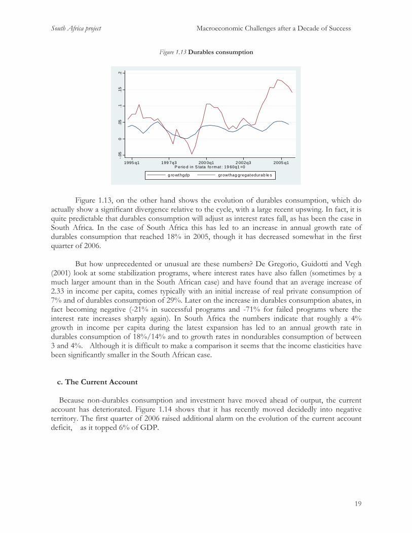
Figure 1.13, on the other hand shows the evolution of durables consumption, which do actually show a significant divergence relative to the cycle, with a large recent upswing. In fact, it is quite predictable that durables consumption will adjust as interest rates fall, as has been the case in South Africa. In the case of South Africa this has led to an increase in annual growth rate of durables consumption that reached 18% in 2005, though it has decreased somewhat in the first quarter of 2006.
But how unprecedented or unusual are these numbers? De Gregorio, Guidotti and Vegh (2001) look at some stabilization programs, where interest rates have also fallen (sometimes by a much larger amount than in the South African case) and have found that an average increase of 2.33 in income per capita, comes typically with an initial increase of real private consumption of 7% and of durables consumption of 29%. Later on the increase in durables consumption abates, in fact becoming negative (-21% in successful programs and -71% for failed programs where the interest rate increases sharply again). In South Africa the numbers indicate that roughly a 4% growth in income per capita during the latest expansion has led to an annual growth rate in durables consumption of 18%/14% and to growth rates in nondurables consumption of between 3 and 4%. Although it is difficult to make a comparison it seems that the income elasticities have been significantly smaller in the South African case. c. The Current Account Because non-durables consumption and investment have moved ahead of output, the current account has deteriorated. Figure 1.14 shows that it has recently moved decidedly into negative territory. The first quarter of 2006 raised additional alarm on the evolution of the current account deficit, as it topped 6% of GDP.
19

South Africa project Macroeconomic Challenges after a Decade of Success
Figure 1.14 The Current Account
-8
-6
-4
-2
0
2
4
6
1989
/02
1990
/01
1990
/04
1991
/03
1992
/02
1993
/01
1993
/04
1994
/03
1995
/02
1996
/01
1996
/04
1997
/03
1998
/02
1999
/01
1999
/04
2000
/03
2001
/02
2002
/01
2002
/04
2003
/03
2004
/02
2005
/01
2005
/04
Current Account per cent of gdp
Theoretically at least, there is not necessarily anything wrong with running a current account deficit, and many economies have managed to sustain large current account deficits for many years (e.g., Australia). To the extent that the current account is used to smooth consumption in anticipation of future increases in output, or especially to finance investment, there is in principle no reason to worry about a current account imbalance. But to the extent that agents do not fully internalize the costs of their lending, then a current account imbalance may signal the buildup of excessive accumulation of foreign liabilities that will lead to a sharp reversal in the future. Among the ways that agents may fail to internalize fully the costs of their borrowing are that they: expect to be bailed out in a crisis, simply do not understand the intertemporal budget constraint that they face (e.g., due to misleading marketing by financial institutions), or accelerate consumption in anticipation of a collapse of the currency because they believe that the current exchange rate is unsustainable .
Our verbal review of the facts seems to suggest that, whereas investment has been a main driver of the current account increase, it has taken place in the nontradables sector, and that the economy exhibits an increasing current account deficit in spite of a high unemployment rate.7 It follows that an acceleration of growth is poised to deteriorate the current account, potentially into risky territory. d. A simulation
To see how quickly the current account can get out of control we have modeled the South African economy scenario going forward through 2014 using both the Treasury’s macro model and
20
7 While the official statistics indicate a sizable current account deficit, we can also compute the current account “inclusive of dark matter” in the terminology of Hausmann and Sturzenegger (2006), i.e. using annual data for the net income service to estimate a notional stock of net foreign assets the change of which is the current account. Doing this computation we find that South Africa is a net debtor with total net foreign debt that is currently close to one hundred billion US dollars, and when tracking this stock of notional capital through the recent decades we find a significant increase in the net stock of net liabilities in the 70s and 80s and again, consistent with official figures, in 2003/2004. However, when these numbers are expressed as percentage of GDP a different picture emerges, with a substantial reduction in real foreign liabilities between the early 80s the mid 90s (of about 40% of GDP) and an oscillating pattern after that (which seems to be strongly influenced by exchange rate movements). In short while the current account has recently deteriorated and may be on an unsustainable path its balance sheet looks relatively strong.
South Africa project Macroeconomic Challenges after a Decade of Success
BER’s forecasting model. In what follows we present the results from BER’s model, and discuss differences with Treasury’s model where relevant.
We first present a typical ASGI-SA scenario, i.e. one in which the goals of the ASGI-SA in terms of output growth are attained. What does the BER model have to say as to how the economy would evolve in such a path? Figure 1.15 shows the main macro variables: GDP growth, consumption and investment ratios, exports and imports as a percentage of GDP, the current account, fiscal account, the rand and terms of trade8.
What does the model say about external imbalances moving forward? As can be seen in the graphs, the current account keeps roughly in balance, without a significant deterioration relative to 2005 levels. However a more careful look reveals two underlying trends that explain this. First, that this result is driven by a significant increase in increase in corporate, personal and government savings which brings consumption to GDP down by close to 4% throughout the estimation period. It is this reduction in consumption that sustains a sharp increase in corporate savings, while avoiding a deterioration of the current account at current values.
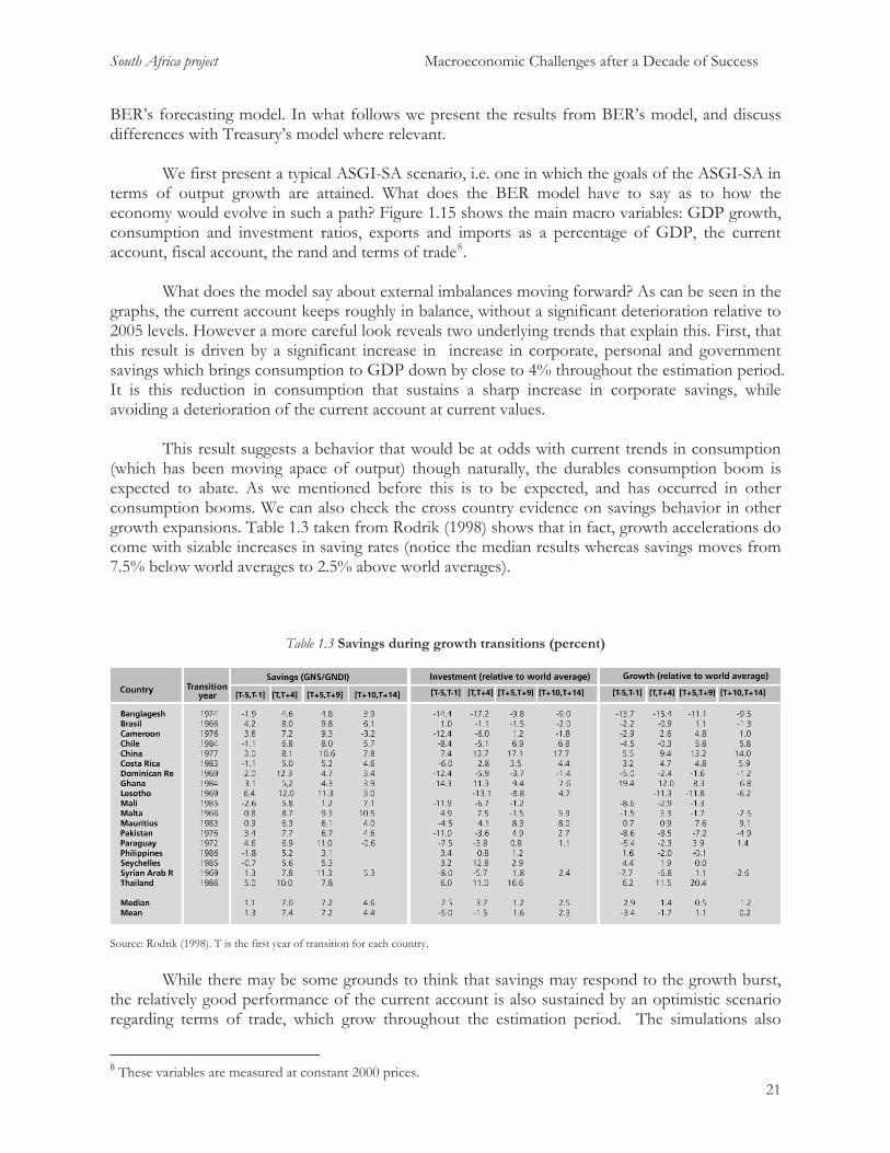
This result suggests a behavior that would be at odds with current trends in consumption (which has been moving apace of output) though naturally, the durables consumption boom is expected to abate. As we mentioned before this is to be expected, and has occurred in other consumption booms. We can also check the cross country evidence on savings behavior in other growth expansions. Table 1.3 taken from Rodrik (1998) shows that in fact, growth accelerations do come with sizable increases in saving rates (notice the median results whereas savings moves from 7.5% below world averages to 2.5% above world averages).
Table 1.3 Savings during growth transitions (percent)
Source: Rodrik (1998). T is the first year of transition for each country.
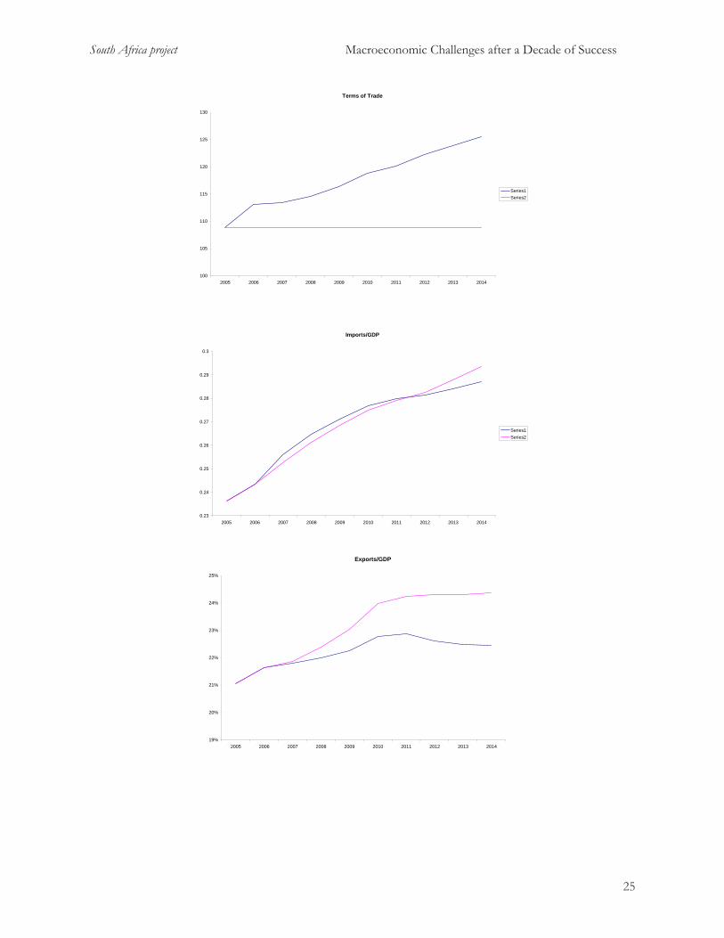
While there may be some grounds to think that savings may respond to the growth burst, the relatively good performance of the current account is also sustained by an optimistic scenario regarding terms of trade, which grow throughout the estimation period. The simulations also
218 These variables are measured at constant 2000 prices.

South Africa project Macroeconomic Challenges after a Decade of Success
indicate a slight deterioration of the government finances, though these remain relatively stable with a deficit below 1% of GDP. The large discrepancy between exports and imports arises from measuring these at constant 2000 prices, while exports benefit from a steady terms of trade improvement. Thus, at current prices the current account remains relatively limited.
Figure 1.15. The basic projection scenario
Growth Rate
0
1
2
3
4
5
6
7
2005 2006 2007 2008 2009 2010 2011 2012 2013 2014 Current Account % GDP
-6
-5
-4
-3
-2
-1
02005 2006 2007 2008 2009 2010 2011 2012 2013 2014
Consumption % GDP
64%
64%
65%
65%
66%
66%
67%
67%
2005 2006 2007 2008 2009 2010 2011 2012 2013 2014 22

South Africa project Macroeconomic Challenges after a Decade of Success
Investment % GDP
0%
5%
10%
15%
20%
25%
30%
2005 2006 2007 2008 2009 2010 2011 2012 2013 2014
Exports and Imports % GDP
0%
5%
10%
15%
20%
25%
30%
35%
40%
2005 2006 2007 2008 2009 2010 2011 2012 2013 2014
Exports Imports
Gov. Deficit % GDP
-1
-0.9
-0.8
-0.7
-0.6
-0.5
-0.4
-0.3
-0.2
-0.1
02005 2006 2007 2008 2009 2010 2011 2012 2013 2014
23

South Africa project Macroeconomic Challenges after a Decade of Success
Rand/US
4
5
6
7
8
9
10
11
12
2005 2006 2007 2008 2009 2010 2011 2012 2013 2014 Source: BER
Figure 1.16 shows, however, the evolution of the main variables in BER’s model if we change the assumption that the terms of trade will continue to improve and replace by the assumption that terms of trade remain at their current levels. As can be seen, this does not affect investment that much, but it does require further decreases in consumption to keep the current account balance in check. Even so the current account balance does deteriorate significantly. All in all we conclude that the economy does exhibit substantial external vulnerability.
Figure 1.16 A simulation with constant terms of trade
Consumption/GDP
61%
62%
63%
64%
65%
66%
67%
2005 2006 2007 2008 2009 2010 2011 2012 2013 2014
Series1Series2
24
South Africa project Macroeconomic Challenges after a Decade of Success
Terms of Trade
100
105
110
115
120
125
130
2005 2006 2007 2008 2009 2010 2011 2012 2013 2014
Series1Series2
Imports/GDP
0.23
0.24
0.25
0.26
0.27
0.28
0.29
0.3
2005 2006 2007 2008 2009 2010 2011 2012 2013 2014
Series1Series2
Exports/GDP
19%
20%
21%
22%
23%
24%
25%
2005 2006 2007 2008 2009 2010 2011 2012 2013 2014
25

South Africa project Macroeconomic Challenges after a Decade of Success
Investment/GDP
16%
17%
18%
19%
20%
21%
22%
23%
24%
25%
26%
2005 2006 2007 2008 2009 2010 2011 2012 2013 2014
Series1Series2
Government Surplus
-0.025
-0.02
-0.015
-0.01
-0.005
02005 2006 2007 2008 2009 2010 2011 2012 2013 2014
Series1Series2
Current Account/GDP
-7
-6
-5
-4
-3
-2
-1
02005 2006 2007 2008 2009 2010 2011 2012 2013 2014
Series1Series2
26

South Africa project Macroeconomic Challenges after a Decade of Success
Rand/US
6
7
8
9
10
11
12
13
2005 2006 2007 2008 2009 2010 2011 2012 2013 2014
Series1Series2
Growth Rate
4
4.5
5
5.5
6
6.5
2005 2006 2007 2008 2009 2010 2011 2012 2013 2014
Series1Series2
Source: BER
3. Why is South Africa running a current account deficit when most emerging markets this time around are running surpluses?
As already noted, South Africa is one of the few countries – along with Turkey, Hungary, and a few others – that has been using the recent boom in capital inflows not just to finance an increase in foreign exchange reserves but also to finance a large current account deficit. Is this cause for concern? Some current account deficits take place for good reasons, others end in crisis. Unfortunately, some have both characteristics. But there is less cause to worry if the recent South African deficits are an adjustment to a new equilibrium based on high-growth fundamentals – whether stimulated by an investment and productivity boom, permanently higher commodity prices, or long-postponed consumption by a newly established black middle class. There is more cause to worry, in light of past historical experience around the world, if the current account deficit is stimulated by temporarily easy credit on world financial markets, excessive government spending, temporarily high commodity prices, or other bubble-like factors. The question whether the current account is too low is closely related to the question whether the rand is too high.
27

South Africa project Macroeconomic Challenges after a Decade of Success
28
a. An estimated exchange rate equation for the rand.
The rand has undergone large movements in recent years. What explains these swings? We now turn to an econometric analysis of the determinants of the exchange rate. Ideally, this would help us form a judgment as to whether the value of the rand in 2006 is appropriate, given economic fundamentals. Somewhat less ambitiously, we would hope to obtain answers to several questions:
• Is the rand a commodity currency, like the Australian and Canadian dollar are said to be (to pick two floaters)? That is, is it a currency that appreciates when prices of the mineral products that it produces are strong on world markets and depreciates when they are weak?
• In other respects, does the rand behave like currencies of industrialized countries, in light of its developed financial markets? (South Africa borrows in rand, for example, unlike most developing countries.) This does not necessarily mean fitting standard theories closely, as those theories don’t work well in practice for major industrialized currencies either. But such variables as GDP and inflation should show up as having an effect.
• Has there been an element of momentum or bandwagon to some recent movements?
Our general equation is: Log Rand value t = α + β 1 Log Real Price Minerals t + β 2 Log (SA GDP/foreign GDP) t
+ β 3 ΔLog Rand value t-1 + β 4 Inflation Differential t + β5 Real Interest Differential t + β6 Country Risk Premium t + β7 trend t + u t .
• We try various versions of this equation: with the value of the rand defined in nominal terms
or real terms, and bilateral against the dollar, or trade weighted. 9 • Real Price Mineralst is computed as a weighted average of the prices of the specific mineral
products that South Africa produces and exports. It is intended to capture the terms of trade, and so is expressed in real form by deflating by the foreign (e.g., US) price level.
• (SA GDP/foreign GDP)t captures an important determinant of the demand for money
(domestic relative to foreign). When the dependent variable is expressed in nominal terms, then the GDPs are expressed in nominal terms (which amounts to imposing the constraint that the elasticity of demand for money with respect to income is 1, as in the quantity theory of money). When the dependent variable is expressed in real terms, then the GDPs are also expressed in real terms. It is only possible to include the GDP variable when we are working with quarterly data; we are forced to drop it when working with monthly data.
• ΔLog Rand Value t-1 is entered experimentally to capture the idea of bandwagon or momentum
elements. • The remaining three variables capture rates of return. It is not enough simply to add interest
rates as a rate of return, and hope for a positive coefficient, because high nominal interest rates in developing countries usually reflect expected inflation, default risk, and devaluation risk.
9Further details on data sources and how these variables were computed are given in the appendix to Frankel (2006b), written as part of this project.

South Africa project Macroeconomic Challenges after a Decade of Success
29
o Expected Inflation Differential (South African minus foreign) should have a negative effect on the expected rate of return to holding rand, and therefore on the demand for rand, and thence on the value of the rand. Here we usually use the one-year lag in the inflation rate to capture the expected future inflation rate. 10
o Real interest differential (nominal interest rate on rand government bonds, minus
expected inflation, minus the same for abroad) should have a positive effect on the perceived rate of return to holding rand assets and therefore on the value of the rand.
o A country risk premium is included to control for risk of default, or risk of future
imposition of capital controls, when looking for a positive coefficient on the real interest differential. Initially we used the spread between the corporate rand interest rate and the government rand rate, under the theory that when default risk raises the South African government interest rates, it raises the corporate interest rate proportionately more, so that this spread is a good proxy for country risk. The preferred measure of the country risk premium is the spread between the interest rate at which South Africa borrows when borrowing in dollars (not rand, because we want to separate out currency risk) and a foreign dollar interest rate of the same maturity. We have been able to obtain also data on the interest rate at which South Africa borrows in dollars, and the corresponding spread with international interest rates, which is a pure measure of country risk or default risk. The data on South African borrowing abroad in dollars is only available since 1996. But the changes that occurred in South Africa in the mid-1990s – the end of apartheid and related opening of the economy and abolition of the dual exchange rate system – were sufficiently fundamental that it is arguably more appropriate to begin the sample period then anyway.
To summarize, the results, which are reported more fully in Frankel (2006b), are highly varied.
But the real commodity price index does appear generally to have the hypothesized positive sign. So does real GDP in the quarterly version (though the real commodity price index and real GDP are sufficiently collinear that they often do not work well when both are included at the same time). Sometimes the lagged rate of change in the exchange rate shows a positive effect, suggesting a bandwagon phenomenon. The results for the rate of return variables are somewhat mixed. The coefficient on the expected inflation differential is not at all statistically significant. The risk variable when proxied by the domestic corporate spread has the hypothesized negative sign and is highly significant statistically. When we use the more appropriate sovereign spread to measure the risk premium, it yields mixed results. The same is true of the real interest differential. Whenever the value of the rand is estimated in level terms, there is a statistically significant negative trend. 11
Here we report one typical version of an equation for the nominal exchange rate, from
monthly data (which requires omitting GDP), as in any country.
10 We have also obtained ex ante measure of inflation expectations from BER forecasts, in place of lagged inflation. But we have not learned a lot from re-estimating the equation with this measure, in part because it is only available quarterly, which requires a big drop in the number of observations. 11 It is probably more appropriate to estimate the equation in terms of changes in the value of the rand, but the results of doing so are generally similar.

South Africa project Macroeconomic Challenges after a Decade of Success
Table 1.4 Exchange rate equation for the value of the rand (79.02-06.07)
The fit, as illustrated in Figure 1.17 for the longer sample period, looks is surprisingly good,
though there appears to be no way of accounting for the magnitude of the depreciation in 2001. But it also shows that the appreciation that followed was very fast and led to an overvaluation relative to the rand’s long run trend. Most importantly for current purposes, the value of the rand in 2006 appears to be in line with what can be explained by traditional macroeconomic determinants, such as the prices of mineral commodities. The depreciation of the rand in May-July 2006 should help somewhat alleviate concerns about an overvalued currency and unsustainable current account deficit.
Figure 1.17: Actual and fitted exchange value of the rand
-0.6
-0.4
-0.2
0.0
0.2
0.4
4
5
6
7
80 82 84 86 88 90 92 94 96 98 00 02 04 06
Residual Actual Fitted
30

South Africa project Macroeconomic Challenges after a Decade of Success
31
Even if the terms of trade have not risen spectacularly – the big rise in prices for South African mineral exports having been substantially offset by a big rise in the price of oil imports – the global commodity boom was nonetheless responsible for the appreciation of the rand over the recent years. The rand has been a “mineral play” for speculators. The reason is that investors have piled into South African assets (especially equities), thus bidding up their price (not only in the form of higher rand prices of equities but also) in the form of an appreciation of the currency. Easy money emanating from the world’s major central banks (Fed, BoJ, ECB, and PBoC) over the period 2001-2005, together with a possible bubble component over the period 2005-06, have probably been one force (the “carry trade”) behind the movement into commodities generally, emerging markets generally, and commodity-based emerging markets in particular.
The bad news is that the bubble component may be especially applicable to South Africa because most other emerging markets are running trade surpluses now. As we will show below a sudden stop would have painful effects on the South African economy, this implies that macro policy needs to pay attention to the current account imbalances. In the end this requires avoiding large real appreciation of the rand, as well as stimulating output with a vigorous growth of the export sector -other parts of this project deal with how to do exactly that.
The spring 2006 financial turmoil depreciated the Rand, an indication that the adjustment
may already be taking place. But, while the rand depreciated somewhat, if the pattern of inflows and appreciation were to resume (i.e., if the reversal of spring 2006 proves to have been temporary), we would support a more active intervention strategy to avoid further appreciation. The reason is that we believe real appreciation of the rand has been an important factor in the large current account deficit.
4. Managing capital outflows in a sudden stop
There are reasons to be sanguine about the odds of a sudden stop or a large depreciation in South Africa. The government is not running large deficits financed by money printing in the context of a fixed exchange rate regime system, the typical setup that often lead to a speculative attack. Nor is the economy apparently suffering from a demand slack resulting from the appreciation of the Rand. Finally, South Africa has a low debt ratio and one that has a relatively high share in domestic currency, thus reducing the possibility of a self fulfilling run generated by fears about the implications of a devaluation on the balance sheets of corporations and the government. In fact in 2001, when the rand/dollar rate almost doubled, growth notched down by just 1.5%, from 4.2% in 2000 to 2001 in 2.7%.
But there are also reasons to worry. Past cycles of large capital inflows to emerging markets
have usually ended in tears. When might it be the turn of South Africa?
a. Could there be a repeat across all emerging markets, as in 1982, and 1997-98?
South Africa has over the last few years experienced large capital inflows, upward pressure on the currency, low spreads on borrowing, upward pressure on securities prices, and faster-than-usual growth. There is a temptation for each country to think that its problems are unique -- and in many ways they are, of course. But the recent macroeconomic situation in South Africa in some respects mirrors that of many other emerging markets around the world. Furthermore, the

South Africa project Macroeconomic Challenges after a Decade of Success
32
entire pattern looks suspiciously like a repeat of two earlier inflow/boom phases that ended, respectively, in the international debt crisis of 1982 and the Asia/Russia crises of 1997-98.
It is probably too early for a full-fledged repeat of those crises. Memories of investors are still too fresh to have allowed themselves to have become over-extended. After all, it was only a few years ago that Argentina agonizingly devalued and defaulted on its debt. Nevertheless, the most recent developments make the question particularly salient. In the spring of 2006, turmoil in international financial markets was triggered by tightened monetary policy in the US, expectations that other major central banks were going to follow suit, and a possible global slowdown.
Thus one must be alert to the possibility of new sudden stops of capital inflow, at least in vulnerable countries. We will first consider the odds of a sudden stop globally, and then consider the vulnerability of the South African economy to such a development.
b. Or have things fundamentally changed?
i. “This time is different”
Two things are striking about the past boom-bust cycles. First, they seem to follow
complete cycles of roughly 15 years. (The same was true in the late 19th century.) Second, when the boom phase is in full swing, most investors develop historical amnesia regarding how past booms ended. Perhaps the reason for the 15-year cycle is that this is how long it takes for those investors who were burned in the last crash to move out of their jobs and to be replaced by investors too young to remember. They know there were crises in the past, but they think “this time is different.”12
ii. More flexible currencies
Having said that, there are a number of respects in which the recent episode of capital
inflows has taken place under more propitious conditions than in the past. The first is that more currencies are flexible than ever before. A floating exchange rate virtually rules out a speculative attack by assumption.13 Exchange rate flexibility deprives speculators of a one-way bet. It also forces firms to confront the possibility of large changes in the exchange rate, and thus discourages them from incurring large unhedged dollar liabilities. To be sure, only a few of the developing countries that claim to be floating are really floating purely, that is, without intervention by the monetary authorities. But the degree of flexibility is higher (with the exception of a handful of small countries that have opted for European integration, dollarization or currency boards).
iii. Higher reserve levels
The second thing that is different this time around is that a far higher fraction of the capital
flows are going into reserves – indeed in many countries the reserves are going up by even more than 100% of capital inflows. This is especially true in Asia, where China has now become the largest holder of foreign exchange reserves in the world and is passing the $1 trillion mark, and among oil producers. Having a high level of reserves – as a ratio, for example, to short-term liabilities – is statistically perhaps the most reliable protection against a currency crisis.14 Indeed,
12 Rogoff (2004) warned that spreads were too low to rationally reflect the chances of another turn in the cycle. 13 Larrain and Velasco (2001) and Levy-Yeyati and Sturzenegger (2001) are two supporters of floating. 14 E.g., Frankel and Rose (1996), Berg, Borensztein, Milesi-Ferreti, and Pattillo (1999) and many others. Such measures as the composition of inflows (e.g., maturity) and the uses to which they are put (e.g., reserves) turn out to be

South Africa project Macroeconomic Challenges after a Decade of Success
33
many economists think that reserves in many developing countries are by now higher than needed.15 Nevertheless the contrast with the past rounds of inflow, which typically went to finance current account deficits more than reserve accumulation16, is striking. (On the current account question, South Africa this time around is one of those that is following the traditional pattern. But more on that below.) In any case, that reserve levels are high globally suggests a low probability of new crises.
iv. Collective Action Clauses
Multilateral discussions to improve the “international financial architecture” accelerated
after the East Asian crisis that began in 1997, although in truth they had been underway at the time of the 1994 Mexican peso crisis and before. Many reform ideas, such as the IMF’s proposed Sovereign Debt Restructuring Mechanism or its Conditional Credit Line either were not adopted or came to little in practice. One proposal, however, has been adopted by countries such as Brazil and Mexico: the inclusion in bond contracts of a Collective Action Clause, which would make it easier to restructure the terms of borrowing in the event of a crisis by preventing a small minority of creditors from blocking such restructurings – in particular, for private sector bonds.17 Thus, like the SDRM and other proposals, it was motivated by the belief that the main failure of international capital markets was an absence of an efficient mechanism, analogous at the domestic level to corporate bankruptcy law, for renegotiating payment terms when adverse developments such as a collapse in exports made it impossible for debtors to pay on the original terms. Others, however, believed that the existing system – conditional new loans from the IMF and sometimes the G7, together with Private Sector Involvement – was working about as well as the system was ever going to work.18 Bonds issued in London, moreover, had always essentially carried the CAC feature. It is not clear that this feature will make much difference in the next crisis, especially for countries that had always borrowed in London.
v. Less dollar-denominated debt
One of the most widely agreed diagnoses of the emerging market crises of the 1990s was that currency mismatch had rendered large devaluations contractionary through the balance sheet effect. This is why output fell sharply following the Mexican devaluation of 1994 and the Asian devaluations of 1997, rather than rising in response to the improved competitiveness of Asian exports. The debts were denominated in dollars (and other foreign currencies), and were unhedged, whereas the revenues of the local corporations and banks were in pesos, baht, won and rupiahs. The result was that after a big devaluation, even otherwise healthy companies were
better predictors of future crises than the simple levels of the aggregate current account deficit or debt. The ratio of reserves to short-term debt captures both aspects. The Guidotti (2003) rule suggests that countries should maintain a level of reserves at least sufficient to cover short term debt, defined as all debt of maturity less than one year or debt otherwise maturing within one year. The motivation is protect themselves against a sudden stop in capital inflows for one year, which should be long enough to generate the needed improvement in the trade balance. 15 Rodrik (2006) says reserves held by developing countries have now climbed to 30% of GDP, or 8 months of imports, and estimates the income loss due to low returns at 1 % of GDP. Also Summers (2006). 16 Calvo, Leiderman, and Reinhart (1996). 17 Eichengreen (1999), Eichengreen and Mody (2000a), Eichengreen and Mody (2000b) Eichengreen and Portes (1995), and Portes (2000 ). See Sturzenegger and Zettelmeyer (2006) for a discussion on whether CACs can mimic the workings of domestic courts. 18 See Roubini (2000) and Frankel and Roubini (2003).
South Africa project Macroeconomic Challenges after a Decade of Success
34
forced to cut back output and employment in order to service their newly-expensive debts, or in some cases to go out of business altogether.
What is the origin of the currency mismatch, the excessive reliance on foreign-currency
denominated debt? An obvious part of the explanation is that foreign investors are reluctant to hold locally-denominated debt out of fear that it will be inflated or devalued away, which has a moral hazard dimension. But devaluation proved in the 1990s as costly to the debtor as to the creditor, which somewhat attenuates the moral hazard danger. And given that the alternative, under dollar-denominated debt, is default, this is not a complete answer to the question why foreigners have been reluctant to hold locally denominated debt. Hausmann attributed it to original sin – an unwillingness of international investors to take open positions in small local currencies that was inherited from history and beyond the control of current policy makers.19 Others attributed it to the illusion of exchange rate stability under declared pegs. 20 A third hypothesis is that the dollar-composition of debt – like the short-term composition – often increases sharply during the brief interval between the month that a sudden stop begins and the month of the ultimate speculative attack, thus worsening the balance sheet effect when the crisis finally arrives.21 The second hypothesis – that currency mismatch is a side-effect of adjustable pegs -- looks better now than it did a decade ago, because many countries have indeed been able to increase the proportion of their debt denominated in their own currencies at the same time as having moved to increased exchange rate flexibility. Regardless the extent to which the flexibility was the cause of the shift in currency composition, the trend is again reassuring.
vi. More openness to FDI and trade
In most countries there has been a continuation of the trend of increased globalization, as
measured for example by the ratio of trade to GDP, despite some setbacks in 2001. A high ratio of trade to GDP is in general good for long term economic growth.22 But it also reduces the frequency and severity of currency crises, according to a number of econometric studies.23
A number of different specific mechanisms have been proposed to flesh out the view, which many find counterintuitive, that openness to trade makes countries less vulnerable to crises. Rose (2002) argues that the threatened penalty of a loss of trade is precisely the answer to the riddle “why do countries so seldom default on their international debts?” and offers empirical evidence that strong trade links are correlated with low default probabilities. International investors will be less likely to pull out of a country with a high trade/GDP ratio, because they know the country is less likely to default. A higher ratio of trade is a form of “giving hostages” that makes a cut-off of lending less likely.24
Another variant of the argument that openness reduces vulnerability takes as the relevant
penalty in a crisis the domestic cost of adjustment, i.e., the difficulty of eliminating a newly-
19 Eichengreen and Hausmann.(1999), and Eichengreen, Hausmann, and Panizza (2003). 20 Eichengreen (1999). 21 Dornbusch (2002), Frankel and Wei (2004), and Frankel (2005). 22 E.g., Frankel and Romer (1999) find that every .01 increase in the ratio (X+M)/GDP raises income over the subsequent 20 years by an estimated 3%. Rodríguez and Rodrik (2001) critique such findings. 23 E.g., Calvo, Izquierdo and Mejia (2003) and Edwards (2004). Cavallo and Frankel (2006) find that openness reduces crises even correcting for endogeneity; that paper also gives further arguments and references, including on the other side of the debate. 24 The point was originally made by Eaton and Gersovitz (1981). They argue that countries that trade more are subject to more harmful trade-related retaliation in the aftermath of default and therefore are less likely to default.

South Africa project Macroeconomic Challenges after a Decade of Success
35
unfinanceable trade deficit. The argument goes back at least to Sachs (1985). He suggested that Asian countries had been less vulnerable to debt crises than Latin American countries -- despite similar debt/GDP ratios -- because they had higher export/GDP ratios. The relatively worse performance observed in Latin America was due to the lower availability of export revenue to service debt. He concluded that: “After a decade of rapid foreign borrowing, too many of Latin America’s resources were in the non exporting sector, or abroad. When financial squeeze in the early 1980’s caused banks to draw their loans, the only way that Latin countries could maintain debt servicing was through a recession and a large reduction in imports combined with debt rescheduling” (p.548). More recently, Guidotti et. al. (2004) make a similar point by providing evidence that economies that trade more recover fairly quickly from the output contraction that usually comes with the sudden stop, while countries that are more closed suffer sharper output contraction and a slower recovery.
Similarly, a high level of inward Foreign Direct Investment generally not only helps raise
long term growth, but also helps reduce the probability of currency crises.25 This is another one of the findings to the effect that the composition of capital inflows matters as much or more than the total in determining the probability of crises:
• FDI is safe, while portfolio inflows are risky; • long-term borrowing is safer, while short-term borrowing is riskier26; • domestic-currency denomination is safe, while foreign currency is riskier; • and all types of equity are safe, while bank loans are risky. Also • concessional loans (e.g., from IDA) are far safer, not because they carry a lower
interest rate (indeed, that can feed the danger of excessive borrowing), but because they tend to be countercyclical, in contrast to market loans.27
FDI has been a relatively high share of the capital inflows in the current decade, just as
bank loans were high in the 1982 episode and bonds in the crises of 1994-2001. In short, the trend toward greater openness with respect to trade and FDI is yet another basis for perhaps believing that “this time is different.”
vii. So, some things are different this time around
Along with the increased exchange rate flexibility, higher propensity to hold reserves, and
lower proportion of dollar-denominated debt, the high levels of FDI and trade augur well for the prospects of getting through the decade without any new economically catastrophic crisis. What are the theories behind these empirical regularities? In each case, one of the easiest rationales to see is that if a country does face a sudden stop of capital inflows, the adjustment is easier, with fewer adverse effects on the real economy. The adjustment is accomplished
• without the deadweight loss of negotiations over debt restructuring and of debt overhang
during this prolonged period, • without the adverse balance sheet effects that higher interest rates have via short-term debt
and that higher exchange rates have via dollar-denominated debt,
25 E.g, Frankel and Rose (1996), among others. 26 Rodrik and Velasco (2000). 27 Frankel and Rose (1996) and Levy Yeyati (2006) among others.

South Africa project Macroeconomic Challenges after a Decade of Success
• and without the sharp fall in output that are necessary – via either large devaluations and large contractions in demand -- to raise a given quantity of export revenue in countries with low ratios of exports to GDP.
On the negative side, for those who view capital controls as having been helpful in the past
(for example, in Chile, Malaysia, India and China), it must be worrisome that capital markets are more open than ever. More importantly, the global economic leadership that was exercised by the G7 and the IMF in the 1980s and 1990s may be missing this time around. The IMF has been attacked from all directions and weakened, while the US government’s style of leadership has since 2001 diverged sharply from the multilateral vision that others have in mind. And reversals in capital flows turn out to be fairly common events. Figure 1.18, borrowed from Guidotti et al (2004), shows that about 8% of non industrial countries do experience reductions in their capital flows of 5% of their GDPs or more. How long will it take until South Africa experiences a reversal?
Figure 1.18. Sudden stops per year as percentage of all countries
Source: Guidotti et al (2004).
36
South Africa project Macroeconomic Challenges after a Decade of Success
37
Summing up, there is less reason to worry now than there was in 1982 or 1997. But crises ultimately are not predictable. Few on the eve of 1982 or 1997 expected a crisis. So the lesson is that one should always be vigilant.
c. Could it happen now?
It was noted above that two or three years into a boom phase seems early for a major correction. Is there any reason to be particularly vigilant at this point in history?
Monetary ease in the US and other major countries contributed to the late-1970s and early-1990s boom phases, and tightening by the Fed in 1980-82 and 1994 helped precipitate the international debt crisis of the 1980s and the Mexican peso crisis, respectively. In both episodes, investors ventured far from home in search of high yields when domestic interest rates fell below what they had become accustomed to, but then scurried back home when US interest rates again rose. The swings in this capital account cycle often exacerbated swings in developing countries’ trade accounts. In theory, when their output and exports are weak, developing countries should be able to borrow on international capital markets to smooth the path of spending. In practice, capital flows in developing countries tend to be procylical rather than countercyclical: global investors only have the confidence needed to lend to developing countries when their economies are booming, and get cold feet when problems develop.
It doesn’t help that the world markets for mineral and agricultural products, as measured by dollar prices, appear to be negatively correlated with real interest rates (see Figure 1.19 below). From the viewpoint of a commodity-producing debtor like South Africa, if international finance becomes scarce at precisely the time that world markets for its exports are weak, then the capital account exacerbates the trade deficit rather than offsetting it. It may not be a coincidence that the commodity booms of the 1970s and 2002-2005 both came at times of globally low real interest rates, while the commodity crash that began in the early 1980s came a time of high real interest rates. Intuitively, high interest rates reduce the demand for storable commodities, or increase the supply, through a variety of channels:
• by increasing the incentive for extraction today rather than tomorrow (think of the rates at which oil is pumped, zinc is mined, forests logged, or livestock herds culled)
• by decreasing firms' desire to carry inventories (think of oil inventories held in tanks) • by encouraging speculators to shift out of commodity contracts (especially spot contracts), and
into treasury bills.
All three mechanisms work to reduce the market price of commodities, as happened when real interest rates were high in the early 1980s. A decrease in real interest rates has the opposite effect, lowering the cost of carrying inventories, and raising commodity prices, as happened during 2002-2004. Call it part of the "carry trade."28 Table 1.5 shows the results obtained from Frankel (2006) for data since 1950. They suggest that on average an increase in real interest rates of 1% typically leads to a fall in commodity prices of about 6%, with an expected half life of 3 years. All results are strongly statistically significant.
Table 1.5 Log Real Commodity Prices and the Real Interest Rates
28 Frankel (2006) presents the theoretical arguments, updated empirical evidence, and further references. Or see http://ksghome.harvard.edu/~jfrankel/CP.htm.

South Africa project Macroeconomic Challenges after a Decade of Success
Figure 1.19 Commodity Prices vs. Real Interest Rate (1950-2003)
Source: Jeff Frankel’s web page
The Fed, BoJ and PBoC had been following extraordinarily easy monetary policies during the beginning of the current boom phase (2002-2004). The Fed returned to raising interest rates in mid-2004. The other major central banks, including the ECB, now appear to be in a period of tightening as well. This raises the question whether investors might once again start pulling their money out of emerging markets.
38
Initially, private investors continued to pour money into assets around the world that seemed to offer a higher rate of return than US Treasury bills: stocks and bonds generally, but especially real estate, emerging markets, and agricultural and mineral commodities. Valuations in all three sectors reached historically high levels, as measured for example by price/rental ratios,
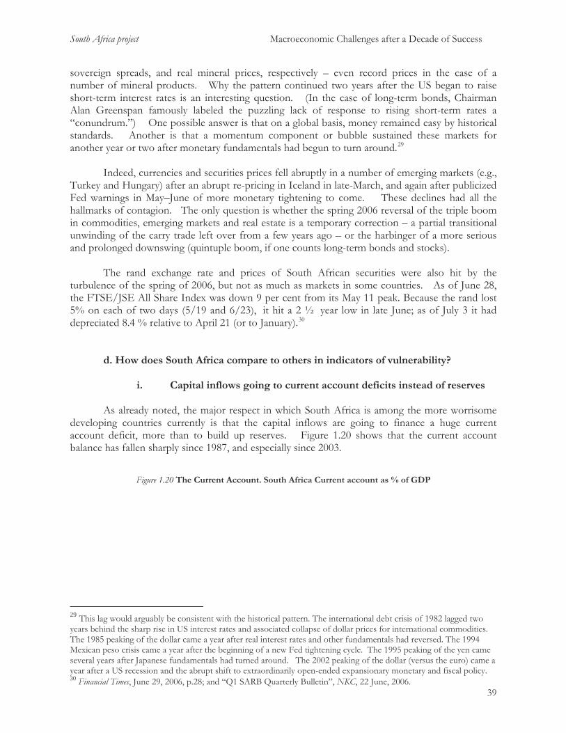
South Africa project Macroeconomic Challenges after a Decade of Success
39
sovereign spreads, and real mineral prices, respectively – even record prices in the case of a number of mineral products. Why the pattern continued two years after the US began to raise short-term interest rates is an interesting question. (In the case of long-term bonds, Chairman Alan Greenspan famously labeled the puzzling lack of response to rising short-term rates a “conundrum.”) One possible answer is that on a global basis, money remained easy by historical standards. Another is that a momentum component or bubble sustained these markets for another year or two after monetary fundamentals had begun to turn around.29
Indeed, currencies and securities prices fell abruptly in a number of emerging markets (e.g.,
Turkey and Hungary) after an abrupt re-pricing in Iceland in late-March, and again after publicized Fed warnings in May–June of more monetary tightening to come. These declines had all the hallmarks of contagion. The only question is whether the spring 2006 reversal of the triple boom in commodities, emerging markets and real estate is a temporary correction – a partial transitional unwinding of the carry trade left over from a few years ago – or the harbinger of a more serious and prolonged downswing (quintuple boom, if one counts long-term bonds and stocks).
The rand exchange rate and prices of South African securities were also hit by the
turbulence of the spring of 2006, but not as much as markets in some countries. As of June 28, the FTSE/JSE All Share Index was down 9 per cent from its May 11 peak. Because the rand lost 5% on each of two days (5/19 and 6/23), it hit a 2 ½ year low in late June; as of July 3 it had depreciated 8.4 % relative to April 21 (or to January).30
d. How does South Africa compare to others in indicators of vulnerability?
i. Capital inflows going to current account deficits instead of reserves
As already noted, the major respect in which South Africa is among the more worrisome developing countries currently is that the capital inflows are going to finance a huge current account deficit, more than to build up reserves. Figure 1.20 shows that the current account balance has fallen sharply since 1987, and especially since 2003.
Figure 1.20 The Current Account. South Africa Current account as % of GDP
29 This lag would arguably be consistent with the historical pattern. The international debt crisis of 1982 lagged two years behind the sharp rise in US interest rates and associated collapse of dollar prices for international commodities. The 1985 peaking of the dollar came a year after real interest rates and other fundamentals had reversed. The 1994 Mexican peso crisis came a year after the beginning of a new Fed tightening cycle. The 1995 peaking of the yen came several years after Japanese fundamentals had turned around. The 2002 peaking of the dollar (versus the euro) came a year after a US recession and the abrupt shift to extraordinarily open-ended expansionary monetary and fiscal policy. 30 Financial Times, June 29, 2006, p.28; and “Q1 SARB Quarterly Bulletin”, NKC, 22 June, 2006.
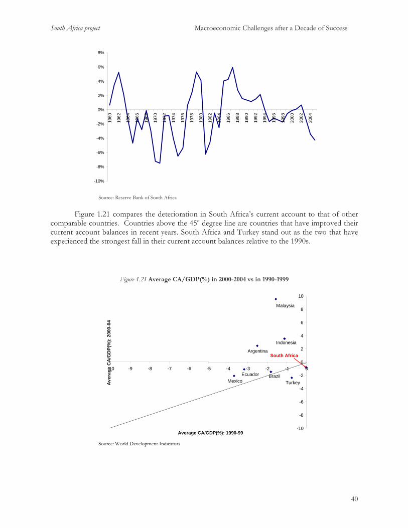
South Africa project Macroeconomic Challenges after a Decade of Success
-10%
-8%
-6%
-4%
-2%
0%
2%
4%
6%
8%
1960
1962
1964
1966
1968
1970
1972
1974
1976
1978
1980
1982
1984
1986
1988
1990
1992
1994
1996
1998
2000
2002
2004
Source: Reserve Bank of South Africa
Figure 1.21 compares the deterioration in South Africa’s current account to that of other comparable countries. Countries above the 45o degree line are countries that have improved their current account balances in recent years. South Africa and Turkey stand out as the two that have experienced the strongest fall in their current account balances relative to the 1990s.
Figure 1.21 Average CA/GDP(%) in 2000-2004 vs in 1990-1999
-10
-8
-6
-4
-2
0
2
4
6
8
10
-10 -9 -8 -7 -6 -5 -4 -3 -2 -1 0
Average CA/GDP(%): 1990-99
Ave
rage
CA
/GD
P(%
): 20
00-0
4
MexicoEcuador Brazil
Turkey
ASouth Africa rgentina
Indonesia
Malaysia
Source: World Development Indicators
40

South Africa project Macroeconomic Challenges after a Decade of Success
ii. Debt levels On the positive side, South African debt levels are not high, perhaps because much of the capital inflow takes the form of equity and FDI. We take debt ratios from Cowan et al (2006), who construct comparable debt ratios across countries. Figure 1.22 focuses on two debt series for South Africa, domestic and external, compared to those for a peer group composed of Argentina, Brazil and Mexico. The numbers indicate that debt to GDP ratios are small in South Africa, and that external debt is relatively minor.
Figure 1.22 Debt characteristics
Debt to GDP ratio
0%
10%
20%
30%
40%
50%
60%
70%
80%
90%
100%
1991 1992 1993 1994 1995 1996 1997 1998 1999 2000 2001 2002 2003 2004
average South Africa
External Debt to Total Debt Ratio
0%
10%
20%
30%
40%
50%
60%
1991 1992 1993 1994 1995 1996 1997 1998 1999 2000 2001 2002 2003 2004
Average South Africa
Returning to the first data source, Figure 1.23-1.25 show that the country still has generally run what is easily the lowest ratio of external debt to GDP of the comparison set, about 20%. Figure 1.25 shows that debt service/exports has fallen to only 10%, the lowest in the group except for export-crazy Malaysia.
41

South Africa project Macroeconomic Challenges after a Decade of Success
Figure 1.23 Average Debt/GDP(%) in 2000-2004 vs in 1990-1999
0
20
40
60
80
100
120
0 10 20 30 40 50 60 70 80 90 100Average Debt/GDP(%): 1990-99
Ave
rage
Deb
t/GD
P(%
): 20
00-0
4 Argentina
42
Source: World Development Indicators
Figure 1.24 South Africa: Debt Service/Export(%)
0
2
4
6
8
10
12
14
16
18
20
1994 1995 1996 1997 1998 1999 2000 2001 2002 2003 2004
Year
Deb
t Ser
vice
/Exp
ort(%
)
Source: World Development Indicators Figure 1.25 Average Debt Service/Export(%) in 2000-2004 versus in 1990-1999
South AfricaMexico
BrazilMalaysia
Turkey IndonesiaEcuador

South Africa project Macroeconomic Challenges after a Decade of Success
0
10
20
30
40
50
60
70
80
0 5 10 15 20 25 30 35 40 45 50 Average DebtSer/Export(%): 1990-99
Ave
rage
Deb
tSer
/Exp
ort(%
): 20
00-0
4
Malaysia
43
Source: World Development Indicators
iii. Exports/GDP ratio
We noted above that openness not only tends to raise the level of income per capita in the
long run, but also reduces the probability of sudden stops and currency crashes in the short run. Trade openness is often measured by exports, total trade, or some measure of the aggregate tradable goods sector, in each case as a ratio to GDP.
Figure 1.26 Export/GDP(%): Comparison among Countries
0
20
40
60
80
100
120
140
1970
1972
1974
1976
1978
1980
1982
1984
1986
1988
1990
1992
1994
1996
1998
2000
2002
2004
ArgentinaBrazilEcuadorIndonesiaMalaysiaMexicoSouth AfricaTurkey
Source: World Development Indicators
South Africa
IndonesiaMexico
Ecuador
Turkey Argentina
Brazil

South Africa project Macroeconomic Challenges after a Decade of Success
Figure 1.27 Average Export/GDP(%) in 2000-04 versus in 1990-99
0
5
10
15
20
25
30
35
40
0 5 10 15 20 25 30 35Average Export/GDP (%): 1990-99
Ave
rage
Exp
ort/G
DP(
%):
2000
-04
Brazil
Argentina
Turkey
Mexico
IndonesiaSouth Africa
Ecuador
Source: World Development Indicators
Figure 1.28 Trade/GDP (%): Comparison among countries
0
50
100
150
200
250
1970
1972
1974
1976
1978
1980
1982
1984
1986
1988
1990
1992
1994
1996
1998
2000
2002
2004
ArgentinaBrazilEcuadorIndonesiaMalaysiaMexicoSouth AfricaTurkey
Source: WDI
44

South Africa project Macroeconomic Challenges after a Decade of Success
Figure 1.29 Average Trade/GDP(%) in 2000-04 versus in 1990-99
0
10
20
30
40
50
60
70
0 10 20 30 40 50 60 70Average Trade/GDP(%) in 1990-99
Ave
rage
Tra
de/G
DP(
%) i
n 20
00-0
4
Brazil
Argentina
TurkeyMexico
Ecuado
Indonesia
rSouth Africa
Source: WDI
Figures 1.26 through 1.29 indicate that South Africa looks moderately open within the comparison set, before we even take account of the remoteness of its geographic location – better than Argentina and Brazil, worse than Malaysia. But Malaysia is the outlier, with one of the highest ratios in the world (after Singapore).
One can use the gravity model of trade to test whether South Africa is more or less open than one would expect from the geographical determinants (size, remoteness, landlockedness, common languages, membership in Free Trade Areas, etc.). This question is relevant because if it is less open than would be predicted by the geographical and other determinants, this strengthens the argument for removal of tariffs and other trade barriers. Figure 1.30 shows countries’ actual ratios of trade to GDP on the vertical axis, and the level that would be predicted by the gravity model on the horizontal axis. As is clearer when we omit the extremely open city states Singapore and Hong Kong from the graph, South Africa’s trade openness is in the middle of the range predicted by the gravity determinants. It is neither as closed as Argentina nor as open as Mozambique, even though all three countries are similarly situated with respect to geographical determinants of trade (e.g., remote from the global economic centers, on the one hand, but with plenty of access to the sea on the other hand).
The policy conclusion remains that trade liberalization would help raise openness, which in
turn would eventually promote growth and reduce the vulnerability to sudden stops. Another way of achieving the goal of increasing openness is to fix the exchange rate or join a currency union.31 While there are other countervailing arguments for keeping the rand flexible against the dollar, euro and other major currencies -- and these arguments will and should continue to dominate – there is the possibility of establishing a southern African currency union, based on the rand or a sort of African version of the EMS or Bretton Woods based on the rand. As long as South Africa can maintain its monetary policy independence, it has to gain from extending the reach of the
45
31 Rose (2000).

South Africa project Macroeconomic Challenges after a Decade of Success
Rand throughout the region. Econometric results suggest that this would boost trade in the region, and overall trade at the same time.
Figure 1.30 Trade/GDP vs. prediction by the geographical determinants in the gravity model
0
50
100
150
200
250
300
350
400
0 0.1 0.2 0.3 0.4 0.5 0.6 0.7 0.8Frankel-Romer-Rose Instrument
Act
ual O
penn
es
Argentina
Belgium
r
Poland
Singapu
Malasia
South AfricaUSA
Hong Kong
Source: Frankel-Romer-Rose variable, available at http://ksghome.harvard.edu/~jfrankel/currentpubsspeeches.htm#On%20Globalization%20and%20Trade
46
0
20
40
60
80
100
120
140
160
180
0 0.02 0.04 0.06 0.08 0.1 0.12Frankel-Romer-Rose Instrument
Act
ual O
penn
es
Argentina
Finland
Indonesia
Madgascar
Mongolia
Mozambique
Malaysia
New Zealand
Papua New Guinea
UruguayUSA
South Africa Mexico
Canada
Burkina Faso
Bolivia Cent Afr Rep
Mali
Australia
Brazil

South Africa project Macroeconomic Challenges after a Decade of Success
iv. Composition of inflow
1. Currency of denomination
South Africa has a reputation for being one of the few developing countries with financial markets so developed that it has long been able to borrow in rand. Figure 1.31 reports the currency denomination of South African foreign debt compared to Argentina, Brazil and Mexico. As can be seen the exposure of South African debt is much smaller than that of a typical emerging country.
Figure 1.31 Foreign Currency Debt
Foreign Currency Debt Share
0%
10%
20%
30%
40%
50%
60%
70%
80%
90%
1994 1995 1996 1997 1998 1999 2000 2001 2002 2003 2004
Average South Africa
2. Equity component versus borrowing
We have examined the share of identifiable net inflows that consist of equity plus FDI (as a fraction of the total that includes bank loans and bonds), for South Africa and the rest of the list of ten comparison countries. One can think of this share as an inverse measure of financial leverage -- as related to a sort of debt/equity ratio. Being net flow numbers, the shares are sometimes less than zero or greater than one. But the fluctuations tend to average out over the 11-year period. 47
South Africa project Macroeconomic Challenges after a Decade of Success
48
Figure 1.32 summarizes the information by putting on the horizontal axis the average share consisting of equity plus FDI, and on the vertical axis the average share over the sample period. Brazil looks very good in terms of both the level and trend in the share of equity and FDI. Of the 10 countries, Indonesia looks the worst. By this measure, South Africa is in the middle: better than the mean or median in terms of the level of the equity share, but with a downward trend. It is surprising that South Africa does not do better in equity and FDI.

South Africa project Macroeconomic Challenges after a Decade of Success
Figure 1.32 Net inflows of equity + FDI as a share of total inflows including borrowing (in %)
(Mean and time trend over the period 1994-
2004)
-15
-10
-5
0
5
10
15
30 40 50 60 70 80 90 100
Average Share of net FDI and Equity flows to total capital inflows (%)
Ann
ual r
ate
of c
hang
e of
the
shar
e
Indonesia
Turkey
Venezuela
Peru
ArgentinaMalaysia Mexico
Brazil
49
Source: Global Development Finance, World Bank
3. Bank debt vs. Bonds
Within the category of “borrowing,” or fixed-income inflows, one can distinguish between bank loans and bond sales. There is a large literature suggesting that countries that rely on the banking system for their inflows are more likely to have crises, perhaps because of a greater tendency toward moral hazard in the form of government bailouts.
Figure 1.33 The percentage share of bonds in total capital inflows (bonds and banks only)
for selected Latin American Countries
0%
10%
20%
30%
40%
50%
60%
70%
80%
90%
1994 1995 1996 1997 1998 1999 2000 2001 2002 2003 2004
Argentina Brazil Mexico Venezuela, RB
Source: Global Development Finance, World Bank
South Africa
Ecuador

South Africa project Macroeconomic Challenges after a Decade of Success
50
The percentage share of bonds in total capital inflows (bonds and banks only) Figure 1.34
for selected Eastern Hemisphere Countries
0%
20%
40%
60%
80%
100%
120%
1994 1995 1996 1997 1998 1999 2000 2001 2002 2003 2004
Indonesia Malaysia South Africa Turkey Source: Global Development Finance, World Bank
4. Short term vs. long term
Figure 1.35 Short term/Long term debt
Figures 1.33 and 1.34 show the relative importance of bonds, versus bank loans, in
combined borrowing, for South Africa and nine other countries. South Africa’s bond share is relatively high in the years since 2000. (These are gross inflows. If one looks at net terms, the country’s net banking inflows appear consistently negative, which seems surprising.) In any case, the lack of reliance on bank inflows seems a good sign.
The final aspect of the composition of the capital inflow is maturity. Short-term borrowing
has been found risky, while long-term inflows much less so. Figure 1.35 suggests that South Africa has always had a low ratio of short-term to long-term debt.

South Africa project Macroeconomic Challenges after a Decade of Success
0
0.02
0.04
0.06
0.08
0.1
0.12
1990
1991
1992
1993
1994
1995
1996
1997
1998
1999
2000
2001
2002
2003
2004
2005
Regardless, there is still room for an improved composition of the debt, especially since
South Africa’s reserves are not that high. Rodrik (2006) has suggested, as a response to the high level of low-return foreign exchange reserves that many developing countries have been accumulating, that paying down short-term debt could be a better use of the funds, since the interest rate charges are higher than what is earned on reserves (US treasury bills). But it would be better still to shift from short-term dollar debt to longer-term bonds denominated in rand. In fact South Africa is close enough to the point of being able to wipe out completely its short term debt.
v. Simulations
To summarize our analysis of the implications for South Africa of a sudden stop we
modeled a sudden reduction in the capital flows to South Africa starting in 2008 32 . While, objections may be raised as to the usefulness of aggregate macro models, we believe they provide a useful reference point to analyze the implications of a sudden stop. Again the simulations were run with two independent macro models typically used to analyze the workings of the South African economy. However we will show here the results from only the BER model macroeconomic forecasting models. 33
Figures 1.36 show the results of a fall in capital flows to zero in 2008, and the response of
the economy to several policy decisions. Scenario 1 allows the rand and interest rates to adjust endogenously, scenario 2 keeps the rand endogenous but assumes the SARB responds by increasing its discount rate by 10% in 2008 and 2009, in scenario 3 this increase is only of 5%, while scenario 4 assumes a 40% depreciation of the Rand in 2008.
The results of all scenarios are fairly similar. The important point is that they show an economy that in spite of being quite prepared, and thus able to avoid a sharp contraction, would still suffer considerably as a result of a sudden stop: growth falls, fiscal accounts deteriorate while consumption and investment fall. These results confirm that this is an important risk that needs to be addressed. 32 The reason we delay the starting point for the sudden stop is to let foreign liabilities increase even further, thus stacking the cards in favor of finding sizable effects.
51
33 One key difference between the BER model shown here and the Treasury model is that Treasury’s model shows a devaluation to improve fiscal accounts.

South Africa project Macroeconomic Challenges after a Decade of Success
Figure 1.36 Simulating a Sudden Stop
BN Capital Flow
0
2
4
6
8
10
12
14
16
18
2005 2006 2007 2008 2009 2010 2011 2012 2013 2014
Baseline Scenario 1 Scenario 2 Scenario 3 Scenario 4
Current Account (% of GDP)
-6
-5
-4
-3
-2
-1
0
1
2
3
4
2005 2006 2007 2008 2009 2010 2011 2012 2013 2014
Baseline Scenario 1 Scenario 2 Scenario 3 Scenario 4
Growth Rate
0
1
2
3
4
5
6
7
2005 2006 2007 2008 2009 2010 2011 2012 2013 2014
Baseline Scenario 1 Scenario 2 Scenario 3 Scenario 4
52

South Africa project Macroeconomic Challenges after a Decade of Success
Consumption (% of GDP)
56%
58%
60%
62%
64%
66%
68%
2005 2006 2007 2008 2009 2010 2011 2012 2013 2014
Baseline Scenario 1 Scenario 2 Scenario 3 Scenario 4
Investment (% of GDP)
16%
17%
18%
19%
20%
21%
22%
23%
24%
25%
26%
2005 2006 2007 2008 2009 2010 2011 2012 2013 2014
Baseline Scenario 1 Scenario 2 Scenario 3 Scenario 4
Exports (% of GDP)
26%
26%
27%
27%
28%
28%
29%
29%
30%
2005 2006 2007 2008 2009 2010 2011 2012 2013 2014
Baseline Scenario 1 Scenario 2 Scenario 3 Scenario 4
53

South Africa project Macroeconomic Challenges after a Decade of Success
Imports (% of GDP)
28%
29%
30%
31%
32%
33%
34%
35%
36%
37%
38%
2005 2006 2007 2008 2009 2010 2011 2012 2013 2014
Baseline Scenario 1 Scenario 2 Scenario 3 Scenario 4
Goverment Deficit (% of GDP)
-7
-6
-5
-4
-3
-2
-1
02005 2006 2007 2008 2009 2010 2011 2012 2013 2014
Baseline Scenario 1 Scenario 2 Scenario 3 Scenario 4
Rand Dollar
4
6
8
10
12
14
16
18
2005 2006 2007 2008 2009 2010 2011 2012 2013 2014
Baseline Scenario 1 Scenario 2 Scenario 3 Scenario 4
54

South Africa project Macroeconomic Challenges after a Decade of Success
Discount Rate
0
2
4
6
8
10
12
14
16
18
20
2005 2006 2007 2008 2009 2010 2011 2012 2013 2014
Baseline Scenario 1 Scenario 2 Scenario 3 Scenario 4
Source: BER
55

South Africa project Macroeconomic Challenges after a Decade of Success
PART 2. THE CONSISTENCY OF THE ASGI-SA PROGRAM
The ASGI-SA strategy begs the question of whether the sought after growth is feasible or not.
We understand feasibility to relate basically to two main constraints. The first refers to whether the amount of resources and their associated productivity levels will be sufficient to deliver the levels of output and growth rates envisioned by the program. The program suggests that investment should be raised from 18% to 25% (at constant prices): are there any grounds to think that the private sector will want to increase investment by as much?, and if not, will/can the public sector fill the gap?, are there sufficiently productive private or public investment opportunities in the economy? These are key questions given the size of the current imbalances of the economy.
The second feasibility question refers to whether the resources can be obtained to finance the increase in investment. Because such a large increase in spending either will put pressure on domestic resources requiring important increases in government and private savings, or, alternatively will lead to important increases in external imbalances. Pressure on domestic resources may increase interest rates, crowding out other projects, or, if it is financed with external resources, the induced vulnerability of the current account will be too big to bear, eventually also leading to an increase in financing costs.
The bottom line is that ASGI-SA should not be seen as a “demand push” strategy. From a
macro perspective the problem is that demand is too high for the productive capacity of the economy (witness its current account deficit). Thus for ASGI-SA to make sense it is critical to think of it as a “supply push” strategy, otherwise it will just worsen the external imbalances of the economy.
In short we see several problems with ASGI. First, that there is little evidence in the program
suggesting that firms will have an incentive to increase investment in the magnitudes required. Second, that it seems to be a program focused on capital deepening when international experience suggests that this is not where the key to growth accelerations lies, more so when even the recent South African experience suggests that capital deepening has not been the most important driver of growth. Finally, that there is no clear explanation of how the resources for the financing of such an ambitious investment program will be obtained without worsening external imbalances. In fact, our previous discussion of scenarios both with growing or stable terms of trade showed a significant deterioration of the current account, even in spite of assuming a declining consumption to GDP ratio.
What does the evidence from other countries have to say on the chances of South Africa to endogenously generate the required resources to sustain the program? Tables 2.1 and 2.2, also taken from Rodrik (1998), shed some light on the issue. Table 2.1 shows how growth and investment respond to savings transitions (defined as substantial and sustained increases in savings rates), while table 2.2 shows how savings responds to growth transitions (defined in a similar way but using growth rates). What can be concluded from both tables is that growth leads to an increase in savings but not necessarily the other way around. In both cases, however, the increase in savings is significantly higher than the increase in investment pointing to the fact that growth accelerations have come hand in hand with improvements in the external balances of the economies involved. Our 56

South Africa project Macroeconomic Challenges after a Decade of Success
forecasts however, seems to suggest that South Africa will see a deterioration of its external picture, rather than an improvement as it moves forward. In addition the above refers to “successful” experiences and thus not clear to what extent it may replicate in an investment led growth strategy. All in all, while there is some likelihood that savings may actually increase we remain relatively skeptical that the problem will just go away on its own.
Table 2.1 Savings transitions
Source: Rodrik (1998).
Table 2.2 Growth Transitions
Source: Rodrik (1998). Table 2.2 also addresses the second question, i.e. what are the required increases in public investment and productivity assumed in the program. Notice that ASGI-SA envisions an increase in the growth rate of roughly two percent, with an increase of investment of roughly 6%, i.e. it requires an increase in investment three times as large as the expected increase in growth rates. Table 2.2 on the contrary shows that in growth accelerations the median increase in growth rate was 6.1% which came about by an increase in investment of 1.7% i.e. the relative “productivity” of investment seems to have been dramatically higher in successful growth transitions than what is envisioned in ASGI-SA. This is confirmed by Jones and Olken (2005) who find that capital at most explains about a third of growth accelerations.
57

South Africa project Macroeconomic Challenges after a Decade of Success
Why is the program set up this way? Table 2.3 is computed assuming both GDP and
investment as exogenous variables, which are taken roughly from the ASGI-SA framework. We use the investment figures to estimate the capital stock assuming a depreciation rate of 6%. Critically, employment is carried forward with the output labor elasticity/productivity growth relations observed during the nineties. Because employment has been stagnant, so is our assumed employment. Productivity is computed as a residual assuming labor and capital shares of 60 and 40%. Figure 2.1 shows that for the program to deliver its growth results productivity needs to continue growing at a fairly brisk pace.34
Figure 2.1 Expected Productivity
4.9
5
5.1
5.2
5.3
5.4
5.5
5.6
4Q2000
2Q2001
4Q2001
2Q2002
4Q2002
2Q2003
4Q2003
2Q2004
4Q2004
2Q2005
4Q2005
2Q2006
4Q2006
2Q2007
4Q2007
2Q2008
4Q2008
2Q2009
4Q2009
2Q2010
4Q2010
2Q2011
4Q2011
2Q2012
4Q2012
2Q2013
4Q2013
2Q2014
4Q2014
In other words, the fact that the combined employment/productivity growth has been so poor implies that if this performance is bound to continue, then the South African project has to rely excessively on capital accumulation. Table 2.2 showed that growth accelerations have been achieved when the economies have been able to include large segments of their population to high productivity jobs. Thus solving the labor market issue is critical to reduce pressure on the capital accumulation process.
What is reasonable to expect from private investment? BER estimates that private investment will go up to about 15.6% of GDP from its current 13.01%. We provide three alternative estimates for the evolution of private investment. One relies on the expected effect of infrastructure investment on private investment. Perkins et al (2005) and Fedderke et al (2006) conclude that there are strong complementarities between public and private investment in South Africa, with private investment increasing typically about 2.37 times a given increase in public investment. In one of our estimations we use this ratio going forward, but still, to achieve the investment goals of ASGI-SA public investment needs to increase a daunting three times from close to its current 14bn Rand to about 41bn Rand. However, these strong complementarities result from the fact that historically large infrastructure investments were needed to develop the mining sector. To the extent that this relationship is not full replicable this may cast some doubts on whether such a strong link may persist in the future. However, the results seem to indicate that
58
34 It is also to be seen if the economy can match recent productivity growth if it actually enters into a growth mode with higher incorporation of labor. Certainly it could, but it would require a challenge much superior to what occurred in the recent past.

South Africa project Macroeconomic Challenges after a Decade of Success
expansions in public infrastructure may have the potential to expand private investments, at least somewhat beyond their current levels.
Table 2.3 Growth estimations
Our second estimate simply assumes that private investment stays at its current share of GDP. In this case public investment needs to increase from 14 billion Rand to about 59 billion Rand. Finally, we estimate an investment function that relates investment to past investment and future growth. In this case the requirements on public investment needs to reach close to 57 billion rand.35
Figure 2.2 Estimates of public investment as % of GDP
4%
5%
6%
7%
8%
9%
10%
11%
12%
1 2 3 4 5 6 7 8 9 10 11 12 13 14 15 16 17 18 19 20 21 22 23 24 25 26 27 28 29 30 31 32 33 34 35 36
With Estimated Investment With Investment at current ratio With Fedderke's complementarity
59
35 The equation relates investment to the last four lags of investment and three forward values of growth. More specifically the equation was Investment = 0.01 + 0.52*** Inv. (-1) + 0.25** Inv. (-2) – 0.14 Inv. (-3) + 0.23** Inv. (-4) + 0.06* Growth (+1) + 0.01 Growth (+2) – 0.04 Growth (+3) + 0.83*** Terms of trade +0.04 RER which was estimated with data since 1960. *,** and *** indicate significance at the 10, 5 and 1% level.

South Africa project Macroeconomic Challenges after a Decade of Success
60
What do we know about the productivity of public investment? Perkins et al (2005) and Fedderke et al (2006) have looked at this issue and found that most items in the infrastructure are granger caused by output and not the other way around, with electricity and roads two exceptions. Fedderke et al (2006) estimates the 2.37 relation above, but also finds that only electricity infrastructure enters separately in the GDP equation with other infrastructure projects having only an effect in terms of stimulating private investment. They also emphasize that the “infrastructure mix” has changed dramatically over time, suggesting that a careful planning of infrastructure is needed if it is to deliver the desired increases in production in the future. Thus, it seems rather difficult to think that public investment will be able to stand up to the challenge of attaining such a large expansion in productive ventures that may stimulate private investment.

South Africa project Macroeconomic Challenges after a Decade of Success
PART 3. FISCAL AND MONETARY POLICY IN A COMMODITY-BASED ECONOMY
1. Inflation targeting and stabilization While simple characterizations never do true honor to the subtleties of macroeconomic policy, the typical description of the policy mix in South Africa would have monetary policy focused on building up nominal credibility through focusing on inflation, with the brunt of the adjustment for macro stabilization on the Central Bank. While we are aware that the monetary authorities are not squarely centered on inflation (witness to this the large accumulation of foreign reserves over the recent years), it is enlightening to transcribe a paragraph from the June 8 meeting of the Monetary Policy Committee: “The international environment has posed increased risks to the inflation outlook. Since the previous meeting of the MPC the exchange rate of the rand has come under pressure as a result of developments in international financial and commodity markets. Previously the relative exchange rate stability had contributed to the positive inflation outlook. In the past weeks, the rand has depreciated against all the major currencies at a time when the US dollar has been weakening against other major currencies. The decline in commodity prices and the re-rating of emerging market risk contributed to the depreciation of the rand from around R6,12 to the US dollar at the time of the previous MPC meeting to current levels of around R6,80, and from R7,42 to the euro to current levels of around R8,65. On a trade-weighted basis, the rand has depreciated by approximately 13 per cent since the previous MPC meeting.” This, among other factors, led to the conclusion “On the basis of the detailed analysis of the economy which is summarized above, the MPC has decided that a moderate adjustment in the repo rate is warranted at present. Accordingly the repo rate is increased by 50 basis points to 7,5 per cent per annum with immediate effect. The MPC will continue to monitor economic developments and all the relevant risks which might have a bearing on the continued attainment of the inflation target.” What is revealing from these paragraphs is the fact that the report focuses on the inflation impact of the reversal in capital flows, and the risk of the rand depreciation’s impact on inflation. This basically suggests a monetary policy that becomes contractionary exactly when capitals are pulling out. This happens to be a well known problem with inflation targeting which we can illustrate with the simplest specification. Imagine a world with supply (s) and demand (d) shocks. We can write output an output equation that depends on both shocks and monetary policy as:
msdy β++= , and inflation as
dsm νωπ +−= . This setup reveals the main dilemma faced by a Central Bank focused on inflation targeting: that demand shocks move inflation and output in the same direction, so that stabilizing one leads to a stabilization of the other, whereas supply shock move output and inflation in different directions. Thus the objective of stabilizing inflation is contradictory with that of stabilizing output. If we 61

South Africa project Macroeconomic Challenges after a Decade of Success
assume the Central Bank chooses m to keep inflation equal to zero (i.e. its objective function is solely focused on inflation), we have
dsm νω −= . This, in turn, implies that
)1()1( βωβ ++−= svdy , which in turn implies that
22222 )1()1( βωσβσσ ++−= sdy v . In short that supply shocks are magnified by the inflation targeting regime, increasing the burden of stabilization on fiscal policy. 2. The fiscal and monetary policy mix in South Africa
The question on the nature of monetary policy in recent years, of course, has been discussed before. Du Plessis and Smith (2003) analyze real interest rates through different phases of the business cycle and have found that monetary policy had been mostly procyclical, though, more recently, du Plessis (2005) has shown that during the 1990s, monetary policy had been more successfully countercyclical while fiscal policy has been modestly countercyclical. This later result is in itself significant as it would show that fiscal policy has escaped the general tendency for procyclicality common in crisis prone emerging economies.
Here we follow a different route, and use a SVAR specification to unveil the nature of monetary shocks. In fact, we will build a model which signals out the effect of monetary shocks and fiscal shocks in addition to supply shocks/external shocks. In fact, this model will allow an assessment of to what extent monetary policy has responded to the other demand shocks and to the other “supply” shocks.
The details are presented in the appendix. In a nutshell, the model estimates
∑∑∞
=−
∞
=−
−
−
=⎥⎥⎥
⎦
⎤
⎢⎢⎢
⎣
⎡
=⎥⎥⎥
⎦
⎤
⎢⎢⎢
⎣
⎡
00..
jjtj
jjt
jt
jt
j
t
t
t
Avds
AConsGovGDP
επ
With, IE ==Σ )'(εε
The identifying restrictions are that fiscal and monetary shocks do not have a long term effect on output, and that monetary disturbances does not affect fiscal policy in the long run.
Figure 3.1 shows the results of the model in terms of the effects of supply shocks, fiscal shocks and monetary shocks on output. The results are very intuitive. Supply shocks have a time lag until they build up to their full effect. Fiscal shocks have a hump shaped form, i.e. it takes about
62

South Africa project Macroeconomic Challenges after a Decade of Success
two years before fiscal shocks reach their maximum effect, which then dies out only after some five years. Monetary shocks, on the other hand have a strong short run effect, but which dies out quickly, i.e. after a year. As a result the variance decomposition implies that for short term macroeconomic management fiscal policy is fairly ineffective, whereas monetary policy is quite effective. In fact, the numbers suggest it is not so much a question of time lags but that fiscal policy simply has a relatively small effect on output. The variance decomposition shows this in Table 3.1.
Figure 3.1 Impulse responses on GDP in the three way model
Supply Shocks
0.00%
0.10%
0.20%
0.30%
0.40%
0.50%
0.60%
0.70%
0.80%
0.90%
1.00%
1 4 7 10 13 16 19 22 25 28 31 34 37 40 43 46 49 52 55 58 61 64 67 70 73 76 79 82 85 88 91 94 97 100 Fiscal Shocks
-0.10%
-0.05%
0.00%
0.05%
0.10%
0.15%
1 4 7 10 13 16 19 22 25 28 31 34 37 40 43 46 49 52 55 58 61 64 67 70 73 76 79 82 85 88 91 94 97 100
Monetary Shocks
-0.10%
-0.05%
0.00%
0.05%
0.10%
0.15%
0.20%
0.25%
0.30%
0.35%
1 4 7 10 13 16 19 22 25 28 31 34 37 40 43 46 49 52 55 58 61 64 67 70 73 76 79 82 85 88 91 94 97 100
63

South Africa project Macroeconomic Challenges after a Decade of Success
Table 3.1 Variance decompositions
To what extent do our shocks truly capture macroeconomic policy in South Africa? We
can compute the component of GDP that is explained by each of the three shocks. These are presented in Figure 3.2.
Figures 3.2 Historical Decompositions
Supply Socks
-5.00%
-4.50%
-4.00%
-3.50%
-3.00%
-2.50%
-2.00%
-1.50%
-1.00%
-0.50%
0.00%
0.50%
1995:01
1995:03
1996:01
1996:03
1997:01
1997:03
1998:01
1998:03
1999:01
1999:03
2000:01
2000:03
2001:01
2001:03
2002:01
2002:03
2003:01
2003:03
2004:01
2004:03
2005:01
2005:03
Fiscal Shocks
-1.00%
-0.80%
-0.60%
-0.40%
-0.20%
0.00%
0.20%
0.40%
0.60%
1995:01
1995:03
1996:01
1996:03
1997:01
1997:03
1998:01
1998:03
1999:01
1999:03
2000:01
2000:03
2001:01
2001:03
2002:01
2002:03
2003:01
2003:03
2004:01
2004:03
2005:01
2005:03
64

South Africa project Macroeconomic Challenges after a Decade of Success
Monetary Shocks
-0.50%
0.00%
0.50%
1.00%
1.50%
2.00%
2.50%
3.00%
3.50%
1995:01
1995:03
1996:01
1996:03
1997:01
1997:03
1998:01
1998:03
1999:01
1999:03
2000:01
2000:03
2001:01
2001:03
2002:01
2002:03
2003:01
2003:03
2004:01
2004:03
2005:01
2005:03
In order to find out if these representations “make sense” we show in figure 3.3 both fiscal and monetary shocks superimposed with the fiscal deficit and with the inverse of real discount rate. In fact the fit is fairly good, our measure of fiscal policy, shown in the left side of Figure 3.3, shows that our demand shocks decrease when the deficit falls and increases when the budget weakens, in spite of the fact that the budget is not used at all to compute these numbers. A discrepancy arises, however, towards the end, with demand shocks increasing in spite of an improving budget. We believe this captures the independent demand shock to investment and durables consumption. Regarding monetary policy the fit is also reasonable, with our monetary policy measure typically expanding when the real interest rate declines.
Figure 3.3 Fiscal and monetary shocks with actual policy
-1.00%
-0.80%
-0.60%
-0.40%
-0.20%
0.00%
0.20%
0.40%
0.60%
1997
/02
1997
/03
1997
/04
1998
/01
1998
/02
1998
/03
1998
/04
1999
/01
1999
/02
1999
/03
1999
/04
2000
/01
2000
/02
2000
/03
2000
/04
2001
/01
2001
/02
2001
/03
2001
/04
2002
/01
2002
/02
2002
/03
2002
/04
2003
/01
2003
/02
2003
/03
2003
/04
2004
/01
2004
/02
2004
/03
2004
/04
2005
/01
2005
/02
2005
/03
0
1
2
3
4
5
6
Fiscal Component of GDP Fiscal Deficit as % GDP"
65
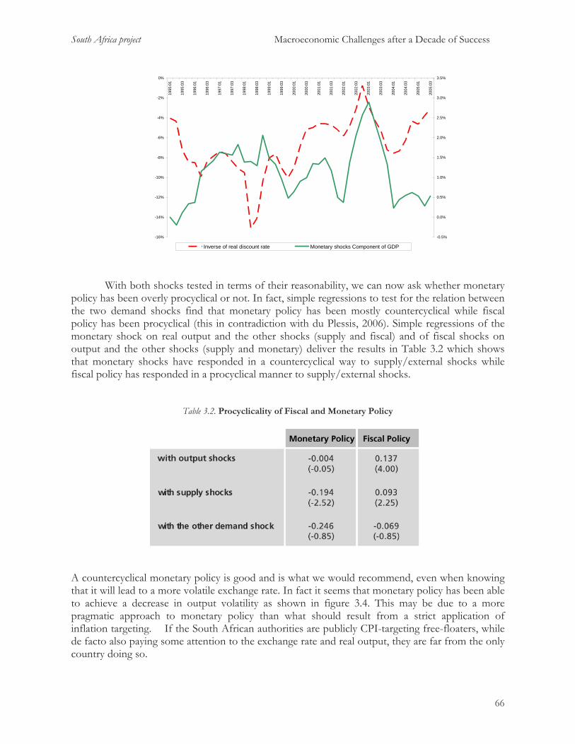
South Africa project Macroeconomic Challenges after a Decade of Success
-16%
-14%
-12%
-10%
-8%
-6%
-4%
-2%
0%
1995
:01
1995
:03
1996
:01
1996
:03
1997
:01
1997
:03
1998
:01
1998
:03
1999
:01
1999
:03
2000
:01
2000
:03
2001
:01
2001
:03
2002
:01
2002
:03
2003
:01
2003
:03
2004
:01
2004
:03
2005
:01
2005
:03
-0.5%
0.0%
0.5%
1.0%
1.5%
2.0%
2.5%
3.0%
3.5%
Inverse of real discount rate Monetary shocks Component of GDP
With both shocks tested in terms of their reasonability, we can now ask whether monetary
policy has been overly procyclical or not. In fact, simple regressions to test for the relation between the two demand shocks find that monetary policy has been mostly countercyclical while fiscal policy has been procyclical (this in contradiction with du Plessis, 2006). Simple regressions of the monetary shock on real output and the other shocks (supply and fiscal) and of fiscal shocks on output and the other shocks (supply and monetary) deliver the results in Table 3.2 which shows that monetary shocks have responded in a countercyclical way to supply/external shocks while fiscal policy has responded in a procyclical manner to supply/external shocks.
Table 3.2. Procyclicality of Fiscal and Monetary Policy
A countercyclical monetary policy is good and is what we would recommend, even when knowing that it will lead to a more volatile exchange rate. In fact it seems that monetary policy has been able to achieve a decrease in output volatility as shown in figure 3.4. This may be due to a more pragmatic approach to monetary policy than what should result from a strict application of inflation targeting. If the South African authorities are publicly CPI-targeting free-floaters, while de facto also paying some attention to the exchange rate and real output, they are far from the only country doing so.
66

South Africa project Macroeconomic Challenges after a Decade of Success
Figure 3.4. Output and inflation volatility
0.00%
0.20%
0.40%
0.60%
0.80%
1.00%
1.20%
1.40%
1994q1
1994q3
1995q1
1995q3
1996q1
1996q3
1997q1
1997q3
1998q1
1998q3
1999q1
1999q3
2000q1
2000q3
2001q1
2001q3
2002q1
2002q3
2003q1
2003q3
2004q1
2004q3
2005q1
2005q3
Inflation Output At any rate, from a macro perspective, the role of monetary policy will be eased if fiscal policy, rather than being procyclical becomes countercyclical itself. We now address this issue.
3. Thinking about the procyclicality of fiscal policy36 It is well known that fiscal policy is fairly procyclical in most developing countries. Why is this so? Among the reasons are:
• Political business cycle, especially in new democracies37 • Need for fiscal contraction in debtors hit by sudden stops.38 • Procyclical capital flows, in emerging markets39 • Dutch Disease, in commodity-producers
Drazen and Brender (2005) analyze the political budget cycle, and suggest that
“the finding of a political fiscal cycle is driven by the experience of "new democracies", where fiscal manipulation may “work” because of lack of experience with electoral politics or lack of information that voters in more established democracies use. The strong fiscal cycle in those countries accounts for the finding of a fiscal cycle in larger samples that include these countries. Once these countries are removed from the larger sample, the political fiscal cycle disappears.”
36 We thank Philippe Aghion for sharing this material with us. 37 Drazen and Brender (2005). 38 Gavin et al (1996).
6739 Kaminski, Reinhart, and Vegh (2004).

South Africa project Macroeconomic Challenges after a Decade of Success
Gavin et al (1996) suggest that the procyclicality arises from limited access to capital markets during downturns, thus forcing the government to contract expenditures when it needs them most. This interpretation finds some support in that spending appears to be much more procyclical during recessions than during booms.
Talvi and Vegh (2000) argue that fiscal policies are procyclical because weak governments cannot face the political pressures to increase spending when in a boom, i.e. when tax collection is on the rise or the economy benefits from an improvement in its terms of trade. Therefore, governments increase expenditures and reduce taxation in order to fend off such pressure, which delivers the result that both tax and expenditure policies become procyclical. The strong increase in fiscal demands during expansions can be rationalized by the so called “voracity effect” proposed by Lane and Tornell (1998). According to their interpretation, if a group does not increase its appropriation during a boom, other groups will. Lane and Tornell show that there is a strong incentive to grab part of the newly available resources before other groups do, and that the incentives to do so increase with the size of the pie; thus, this common pool problem becomes stronger in an expansion delivering the procyclical result.
One variant of this source of procyclical fiscal policy is the Dutch Disease. In commodity booms governments increase spending – e.g., on government employment -- in response to the greater availability of finance through both tax revenue and borrowing. Then they find it hard to cut back when commodity prices go back down. The accompanying figures for oil exporters Indonesia and Iran show how their public wage bills (employment times wage) depend heavily on the real price of oil, an effect that is still strong three years lagged.
Figure 3.5 Government wage bill (as percent of GDP) vs. real oil price
Indonesia
IND
Wag
e Ex
pend
iture
as
% o
f GD
P
Real Oil Prices lagged by 3 year, in Today's Dollars11.46 59.88
1.77
3.52
Iran
68
IRN
Wag
e Ex
pend
iture
as
% o
f GD
P
Real Oil Prices lagged by 3 year, in Today's Dollars11.46
7.4
16.52
59.88

South Africa project Macroeconomic Challenges after a Decade of Success
69
More recent work by Aghion et al (2006a, 2006b) has studied the link between fiscal policy procyclicality and growth. This work challenges the accepted view that “the only link between macro-policy and long-run growth…is that growth requires macroeconomic stability everything else remaining equal” (see Aghion et al, 2006b, p.1) because this argument assumes firms could always borrow enough funds to either reorganize their activities or move to new activities/markets (as workers could relocate from one job to another) during the business cycle. If so, recessions have a cleansing effect of reallocating resources in a way that maximizes overall productivity, leading to the recommendation that governments should better avoid intervention in the process (beyond insuring macro stability).
Suppose, however, that borrowing capacity for domestic firms is constrained at least for a subset of them. In this case, firms will be unduly constrained during a recession, and there may be a role for macro-policies. In fact, a countercyclical budgetary policy may mute the negative consequences of a recession (or of a bad aggregate shock), for example, on firms’ innovative investments. It follows that the lower the level of financial development (the tighter the credit constraints), the more growth-enhancing such countercyclical policies should be.
To the extent that at least some South African firms are credit constrained, we have a case for countercyclical budgetary policies. In practice, the government may increase the volume on public investments, thereby fostering the demand for private firms’ products during recessions and by propping up their cash flow allowing them to avoid the credit constraint, and avoiding sacrifices to R&D or other productivity enhancing investments.
Following Aghion et al (2006a, 2006b) we measure the procyclicality of fiscal policy by computing a rolling regression which relates the reaction of fiscal policy to output shocks.40 Figure 3.6 shows a measure of the rolling coefficients throughout recent South African history for public investment, public consumption and government debt. Consistent with our numbers above, fiscal policy seems to have a mildly procyclical pattern.
We then estimate the relation between procyclicality and growth. The results are summarized in table 3.3, which based on the above-mentioned arguments, show that by reducing public investment procyclicality would increase growth by 0.36% per year. Similar results obtain when analyzing government consumption or debt. Thus, our main policy recommendation on this issue would be the need of a countercyclical fiscal policy.41
Our preferred way of obtaining such procyclical fiscal policy, is to fix the level of public
expenditure on the basis of long run objectives in terms of public goods (at any rate fiscal policy is relatively inefficient for short run macro stabilization) while allowing for public resources to move with the cycle. These automatic countercyclical mechanisms in the budget are likely to deliver better growth performance.
40 The rolling regression includes a ten year window centered at each moment in time. 41 While we would expect the growth effect to decrease with the level of financial development we find the opposite result for investment and debt for South Africa which may be related to the high degree of financial development. At any rate the overall result provides the relevant estimator.

South Africa project Macroeconomic Challenges after a Decade of Success
Figure 3.6. Rolling regressions on procyclicality
-0.6
-0.4
-0.2
0
0.2
0.4
0.6
0.8
1
1.2
1965
1966
1967
1968
1969
1970
1971
1972
1973
1974
1975
1976
1977
1978
1979
1980
1981
1982
1983
1984
1985
1986
1987
1988
1989
1990
1991
1992
1993
1994
1995
1996
1997
1998
1999
2000
Year
Estim
ated
cyc
lical
ity in
Pub
lic In
vest
men
t
-2
-1
0
1
2
3
1965
1966
1967
1968
196919
701971
1972
1973
1974
1975
1976
1977
197819
79198
0198
119
8219
8319
841985
19861987
1988
1989
1990
1991
1992
1993
19941995
1996
1997
1998
1999
2000
Year
Estim
ated
cyc
lical
ity in
Gov
. Con
sum
ptio
n
-7
-6
-5
-4
-3
-2
-1
0
1
1965
1966
1967
1968
1969197
01971
1972
1973
1974
1975
1976
1977
197819
79198
0198
119
8219
8319
841985
19861987
1988
1989
1990
1991
1992
19931994
1995199
619
9719
9819
9920
00
Year
Estim
ated
cyc
lical
ity in
Pub
lic D
ebt
70

South Africa project Macroeconomic Challenges after a Decade of Success
Table 3.3 The effects of procyclicality on growth
4. Options for managing fiscal policy
a. The design of fiscal policy in a commodity-exporting country
As noted, one of the standard Dutch Disease problems is excessive growth in spending by
the government which is hard to reverse when the cycle goes back down, either because the economy slows down or some income tax commodity based revenues fall. A question for South Africa today is: if “spending the surplus” is a political constraint, can institutions be phrased so as to minimize such undesirable Dutch Disease dangers? One possibility is to aim for a fiscal policy that targets a cyclically adjusted budget outcome. What this budget outcome should be depends on how the government sees its intertemporal budget constraint. Chile for example, aims at a budget surplus to compensate (1% of GDP) for the fact that it is depleting its stock of mineral resources.
The way to implement this cyclically adjusted fiscal policy would be to have a relatively flat
spending profile while taxes would move procyclically, generating an automatic countercyclical fiscal policy. Notice that we are careful not to talk about fiscal rules; South African authorities have worked hard to earn credibility which has the benefit of allowing some margin of discretion. What would then be the logic of constraining themselves with fiscal rules which are just bound to be violated when shocks require the use of discretion?
While of limited importance for South Africa, where the South African government does
not own the mineral resources directly, one could also think of mechanisms such as a “Mineral Revenue Stabilization fund.” It is true that in the case of South Africa, the share of revenues coming from the mining sector is relatively small, but this does not preclude large swings in commodity prices that may affect the income tax collected from the sector. A panel of independent experts could be established to estimate how much of tax revenue is due to temporary commodity price boom, after which that amount is to be put aside rather than spent. To enhance the acceptability of the idea from a political economy viewpoint, the money could go into an account earmarked it for retirement funds or to run down debt. Also it may be possible to use the argument that non-renewable resources are being run down.
b. Debt management for reduced vulnerability
Without passing judgment on the probability or severity that any future financial crisis
could bring South Africa, or any country, it useful to think of ways that policy makers might be able to reduce the probability and severity of such crises. The big questions of budget deficits, saving, overall levels of debt, and monetary policy are discussed in other parts of this report. Here we largely take the budget deficit and national saving as given. To begin with we even take the
71
South Africa project Macroeconomic Challenges after a Decade of Success
72
current account deficit as given, and ask a more technical question: for a given overall magnitude of capital inflow, can ways be found through debt management to reduce the probability and severity of possible crises.
i. The composition of inflows and better risk-sharing
We have already seen that, even taking the total of capital inflows as given, the composition can make a big difference. The different dimensions of composition have in common that the more desirable arrangements are those that efficiently allow the country to share risks with foreign investors -- those that automatically divide the losses of bad times – and the gains of good times -- in some reasonable proportion between the two sides. 42 In the case of short-term dollar-denominated loan, “bad times” implies an inability to service the debt on the terms originally agreed to. which some authors have likened to a way to introduce “sharing rules” into typical debt contracts. 43 However, both of the traditional responses by the monetary authorities – devaluation and monetary contraction – have adverse balance sheet effects, and typically there follows a difficult, lengthy and expensive period of negotiation. The restructuring is likely to be difficult and lengthy in part because it may be necessary to try to round up thousands of small creditors (especially in the case of bondholders), many of whom will wish to “free ride” on the concessions of the others. It is likely to be expensive in part because of the time demands on bankers and government officials when they should be devoting attention to the real economy, and in larger part because an existing debt overhang is likely to discourage companies from undertaking new projects out of fear that any foreign exchange profits will be taken away from them to service the old debt. The intent of Collective Action Clauses is to ease the negotiations by reducing the free rider problem, but even if this eases somewhat the pain of the adjustment it is clear that this is not a mechanism to be relied upon.
A more complete answer to the problem is to finance a higher fraction of the inflow in the
form of rand-denominated debt, equity, and foreign direct investment in the first place. Then in the event of bad times, such as a collapse in the world market for the country’s exports, the value of the assets falls automatically, with no negotiation needed. In the case of the rand-denominated debt, the value automatically declines when the rand declines on the foreign exchange market. In the case of equity and FDI, the value of the assets automatically declines for a second reason as well: the decline in the share value of the company expressed in rand.
South Africa has long been fortunate to be able to borrow in rand, in part because its
financial markets are generally well-developed, and fortunate to experience large FDI inflows, in part because of attractive opportunities in the natural resource sector. Still, further movement in this direction is both possible and desirable.
ii. A proposal to link bonds to mineral commodity prices
Financial markets have come up with hundreds of innovative derivative contracts and other financial products with the presumed goal of helping managing risk. It is a great puzzle for macroeconomists who think about the problems of mineral-exporting countries why the existing
42 In theory, in well-functioning international financial markets, idiosyncratic country risk should be borne entirely by global investors. The reality seldom works that way, however, and in any case much of the risk we are talking about is not idiosyncratic but global. 43 E.g., see Grossman and Van Huyck (1988.)
South Africa project Macroeconomic Challenges after a Decade of Success
73
list of successful financial instruments does not include commodity-linked bonds.44 In theory, linking the value of bonds to the price of gold or platinum or a basket of minerals could constitute an additional interesting instrument to the risk-sharing problem for a mineral exporter such as South Africa45. When the dollar prices of those commodities decline on world markets, the dollar price of the liabilities would automatically decline in proportion. The arrangement is better than linking bonds to GDP, another academic proposal that has seemingly attracted more support, because the price of minerals can be measured more precisely and is not subject to subsequent revision as is GDP, nor to any moral hazard risk. It is even better than equities and FDI in that not all developing countries have sufficiently high transparency of accounting, integrity of management, and security of property rights to give foreign investors complete confidence. Particularly among petroleum exporters like Russia, the accounting and corporate governance is sometimes even worse than Enron’s.
Mexico is one country that has experimented with hedging its oil exports by selling oil futures.46 In theory this should be the same as shifting the composition of borrowing from dollars to oil. (Or, if borrowing was previously in the domestic currency, then selling oil futures should be the same as shifting to oil-denomination plus also buying peso futures.) In practice, there seems to be a subtle but critical difference between the futures strategy and the strategy of issuing mineral-linked bonds. The difference has to do with the career of the minister or vice-minister of finance. Assume the price of oil goes up. The rest of the country comes to him expectantly, dreaming about how to use the windfall gain in wealth. If the minister has previously sold oil futures, and has to tell them there is no gain to spend, his career prospects are in jeopardy. The disappointment sharpens when the news enters the public domain: “Oil Minister Gambles Away National Patrimony on the Futures Market.” Assume the price of oil goes down. The finance minister who has hedged on the oil futures market may just have saved his country from disaster, but nobody notices. Denominating bonds in the price of the export commodity largely avoids this career risk problem.
Economists in countries like Chile have discussed this option (denominating loans in
copper, in their case). But it has never caught on. The usual answer is that Wall Street investors have not shown interest. This is surprising. Bonds denominated in copper or gold or oil have a natural buy-side constituency – companies that need to buy copper or gold or oil as inputs into production, for whom these bonds are a natural hedge. It seems likely that the problem is that because financial markets require liquidity, a new one will not be successful unless there is an initial push that gets it past a certain size threshold. Perhaps it is time to try to start a market in platinum bonds (or re-start a market in gold bonds, which do have a long history). It might take a major effort – e.g, a refusal to borrow on other terms and/or coordination among a number of
44 Commodity-linked bonds have been proposed many times. The earliest modern-day reference known to the authors is Lessard and Williamson (1985). 45 It could be discussed how relevant this proposal is for South Africa given that SA faces no material risk of fiscal strain from a decline in the international price of any (or even all) of its major export commodities, that gold (and platinum) are comparatively small sectors of the SA economy and that a mineral linked bond would make more sense for an economy where (i) the ability of the government to service its debt was closely tied to commodity revenues and (ii) the same government faced liquidity constraints which prevented it from smoothing over rough times while neither of these conditions holds for South Africa. And then there is the question of whether this has better hedging properties than jut borrowing in Rands. Our approach in this section is to just suggest that this may provide a new complementary form of financing that is worth exploring. At any rate it will be key to find out if such proposal is financially convenient or entail interest costs that make it “too expensive”. 46 It has also recently issued insurance protection in the form of issuing debt in which the capital is not payable if a large hurricane hits the economy.

South Africa project Macroeconomic Challenges after a Decade of Success
borrowing countries and creditor institutions -- to overcome the liquidity threshold effect and the apparent traditional reluctance of foreign investors. But a time when both mineral commodities and emerging markets are “hot” is probably a good time to inaugurate such an instrument.
An illustrative example to show that liquidity market matters is the fate of the GDP linked
bond issued at the time of the Argentine restructuring. While the instrument did not trade it was “valued” at 2 dollars. In the initial trading rounds this was the actual trading price. However as soon as liquidity moved up the price increased continuously and nowadays hovers around 9 cents on the dollar (see figure 3.6). It does seem that liquidity does matter. 47
Figure 3.6 The Argentine GDP linked bond (in US dollars)
4
5
6
7
8
9
10
11
11/3
0/20
05
12/7
/200
5
12/1
4/20
05
12/2
1/20
05
12/2
8/20
05
1/4/
2006
1/11
/200
6
1/18
/200
6
1/25
/200
6
2/1/
2006
2/8/
2006
2/15
/200
6
2/22
/200
6
3/1/
2006
3/8/
2006
3/15
/200
6
3/22
/200
6
3/29
/200
6
4/5/
2006
4/12
/200
6
4/19
/200
6
4/26
/200
6
5/3/
2006
5/10
/200
6
5/17
/200
6
5/24
/200
6
5/31
/200
6
6/7/
2006
6/14
/200
6
6/21
/200
6
6/28
/200
6DOLAR EURO PESOS
Source: Bloomberg.
74
47 Unfortunately this experience may be of limited interest, in that Argentina issued a very large amount of these instruments during its debt restructuring. Such large issues are not replicable for new bonds.

South Africa project Macroeconomic Challenges after a Decade of Success
PART 4. ALTERNATIVE WAYS TO MANAGE INFLOWS, AND THE EXCHANGE RATE REGIME
In this section we consider the flip side of our concern on sudden stops, to discuss the
dilemmas of monetary policy when an economy faces significant capital flows, and how this relates to the longer-run choice of exchange rate regimes.
Amost as a matter of definition, a country experiencing a balance of payments surplus or a
an increase in demand for its assets has a basic choice, among (i) allowing the currency to appreciate, (ii) intervening to keep the value of the currency down, low or (iii) some combination of the two.
1. Allow appreciation
a. Has the float allowed the rand to become overvalued? Here we note that the South African monetary authorities, as those in most countries that have recently experienced large inflows, have taken the increased demand partly in the form of a higher price (an appreciation of the rand) and partly in the form of a greater supply (more rand assets issued by the Reserve Bank). The proportion of the “exchange market pressure” that shows up in the form of appreciation is less than one might think from the official description of the regime as floating. South Africa shares this property with most other self-described floaters.48 But the tendency to intervene also looks substantially greater than that of four other commodity-exporting inflation-targeting floaters: Brazil, Australia, Canada and New Zealand. The authors of this report, despite agreeing on the need for a flexible exchange rate, believe this is probably to the good. We first explain why, and then consider frameworks for intervention.
75
48 This is the famous “Fear of floating” of Calvo and Reinhart (2002).

South Africa project Macroeconomic Challenges after a Decade of Success
Figure 4.1 Propensity to float, and variability of exchange rate
76
0
2
4
6
8
10
12
14
- 0.2 0.0 0.2 0.4 0.6 0.8 1.0 1.2 1.4 1.6 1.8 Propensity to float: % change in ER / (% change in ER + % change in RES) averaged over 2000Q1-2006Q1
rate
b. Arguments for avoiding overvaluation
i. The Dutch Disease
One argument for avoiding overvaluation is that the boom may be temporary but pvate agents do not realize it. The combination is what makes the Dutch Disease a disease. The Dutch Disease can be defined as balance of payments inflows – originally those based on a commodity boom – putting pressure on the real exchange rate, with various inconvenient side effects. The inconvenient side effects range from crowding out of non-commodity exports, to large international debt, to irresistible political temptations for the government to spend the money. Despite these inconvenient effects, the “disease” is not necessarily undesirable. If the private economy is going to respond to price signals by moving into commodities, then it has to move out of somewhere, after all. What makes the pattern truly a disease if the boom proves to be temporary, in a way that was not adequately foreseen. In the worse cases, after the commodity prices reverse the country is left with a decimated manufacturing export sector, an unserviceable debt, and a bloated government that cannot easily be cut back.
ii. Growth effects
This report has taken a relatively open view as to what will happen to capital flows in the
near future. In the earlier part of this report we discussed the risks entailed by the possibility of a sudden stop. But we have also discussed the possibility that at times South Africa (and other emerging countries) will find themselves fighting capital inflows rather than capital outflows. Here we ask whether there is evidence that fighting a real appreciation is effective and whether it has any relevant effect on macro variables. Levy-Yeyati and Sturzenegger (2006) discuss this issue. In a nutshell they look at a cross section of countries, and compute for each of them the level of exchange rate intervention. They then relate the level of these interventions to a series of variables,
China Malaysia
Brazil
Turkey
Japan Canada
Korea Switzerland Norway
Indonesia
New Zealand
India
Chile
South Africa
ustralia A

South Africa project Macroeconomic Challenges after a Decade of Success
the ratio of the current and future exchange rate, as well as to export and GDP growth. They test whether countries that have intervened can achieve higher growth rates by sustaining more depreciated currencies. Their results, robust to a series of specifications, seem to suggest that:
1. Countries that actively intervene to prevent an appreciation are, in fact, able to sustain more depreciated currencies rates than in the subsequent years, 2. Intervention seems to be correlated with higher growth rates in the immediate aftermath of the intervention (1-3 years) 3. Export growth seems to be stimulated by intervention in the previous four years. 4. These results are robust to the inclusion of time and fixed effect as well as to the use of instrumental variables.
Table 4.1 shows a sample of their results for emerging economies. In one of their
specifications, the one we have chosen to show here, they build an index of interventions which measures the number of years during the current and previous three years that the intervention has been positive (i.e. that the central bank has accumulated foreign reserves). The group of countries includes all those that intervene, i.e. intermediate and peg regimes. The first line shows that the effect of this variable is quite positive and statistically significant, implying a better growth performance both for output and for exports. The finding is strong support for this strategy.
Table 4.1 Intervention and growth
iii. Intervention to add to reserves
Events in the foreign exchange market are changing so rapidly that it is hard to comment prescriptively. But if the inflows of recent years are sustained in the aftermath of the global bout of turbulence of the spring of 2006, we do have a recommendation, namely that the authorities continue to intervene more heavily than is implicit in the official regime of CPI-targeting floater. One goal is to prevent overvaluation, thereby preserving the non-commodity export sector. Another is to add to the stock of reserves, which is not in the excessive range of many Asian countries.
77

South Africa project Macroeconomic Challenges after a Decade of Success
78
Earlier we presented a simple model explaining why we believe that the monetary
authorities should not interpret inflation targeting in a narrow or literal way, particularly in the presence of supply shocks such as sharp increases in the price of oil on world markets. To do so would imply, for example, sufficient monetary contraction to appreciate the currency and prevent oil prices rising in terms of rand, which is not the right response. The right response to an adverse movement in the terms of trade is, if anything, a depreciation, not an appreciation. The many defenders of inflation targeting will protest that is not what is meant by the regime anyway. But, in the first place, transparency and credibility suggest that it be decided ahead of time what price index is to be targeted (e.g., headline CPI, core CPI, Producer Price Index, or export price index), rather than trying to explain deviations from the price index that had been proclaimed. In the second place, inflation-targeting floaters do behave as if their monetary policies tend to respond to increases in dollar prices of oil imports, to follow the example above, not by ignoring them, but by tightening enough to appreciate the currency.49 The bottom line recommendation, again, is to exclude oil prices from CPI target; i.e., not to respond to high dollar oil prices by tightening monetary policy and appreciating the currency so as to keep rand oil prices unchanged.50
2. Intervention to dampen appreciation
The normal alternative to fluctuations in the exchange rate is foreign exchange intervention which, as we have seen, the South African monetary authorities do engage in extensively. Two aspects of intervention have not yet been addressed. First, should the authorities sterilize (what are the costs and limits of sterilization?), or should they just allow the money to flow in. On this first question, the authors feel that even in a country without obvious capital controls, there is some scope for sterilization and it can be useful, especially at early stages of an unexplained capital inflow. After a couple of years, however, sterilizing large inflows becomes increasingly difficult, in part because it often leads to a rising quasi-fiscal deficit.
Figure 4.2 seems to suggest that the South African authorities have let base money increase
more rapidly than many others in the comparison group, such as China, which has sterilized its inflows, and Chile, which has opted to float freely and thus has had no net money inflows to contend with.
49 Frankel (2006a). 50 This lesson is half the argument for the PEP proposal (Peg the Export Price), the argument that improves on CPI targeting. The other half is the argument that improves on a fixed exchange rate: by targeting the export price, the currency automatically appreciates when world markets are strong and depreciates when they are weak, with no painful abandonment of the nominal target. The strict version of PEP would call for South Africa essentially to go back on the gold standard (Frankel, 2002). Under a mild version of PEP, within the existing framework of inflation targeting, the Reserve Bank would simply announce that it is monitoring an index of export prices.

South Africa project Macroeconomic Challenges after a Decade of Success
Figure 4.2 Comparison of % change in Exchange Rates vs % Changes in Dollar amounts of Base Money
79
-150%
-100%
-50%
0%
50%
100%
150%
0.0 0.5 1.0 1.5 2.0 2.5 3.0 3.5 4.0 4.5 5.0
% change in Base Money
% c
hang
e in
Exc
hang
e R
ate
Indonesia
Brazil
Australia
Korea
CanadaNew Zealand
Thailand
Malaysia Chile China
South Africa
Source: International Financial Statistics, IMF The second question is: how much reserves are enough? The traditional denominator for
deciding “how much reserves are enough” used to be imports. As Figure 4.3 shows, South Africa has succeeded in raising its reserves from the disastrously low levels of 1997. But it still has a low ratio of reserves to imports – barely two months’ worth! Figure 4.4 shows that this level is still very low by the standards of other emerging market countries.
Figure 4.3 Reserve in months of imports - South Africa

South Africa project Macroeconomic Challenges after a Decade of Success
0
0.5
1
1.5
2
2.5
3
3.5
4
4.5
1970
1972
1974
1976
1978
1980
1982
1984
1986
1988
1990
1992
1994
1996
1998
2000
2002
2004
Source: World Development Indicators
Figure 4.4 Average Reserve in months of imports in 2000-04 vs in 1990-99
0
1
2
3
4
5
6
7
0 1 2 3 4 5 6 7average resrves in months of imports: 1990-99
Ave
rage
rese
rve
in m
onth
s of
impo
rts:
200
0-04
Mexico
Malaysia
Turkey
Indonesia
Argentina Brazil
South Africa
rEcuado
Source: WDI
4.5 International Reserve/Short Term Debt (%) - South Africa
80

South Africa project Macroeconomic Challenges after a Decade of Success
0
20
40
60
80
100
120
140
160
180
1994 1995 1996 1997 1998 1999 2000 2001 2002 2003 2004
Source: World Development Indicators
Figure 4.6 Average International Reserve/Short term debt (%) in 2000-04 versus 1990-99
0
50
100
150
200
250
300
350
400
450
500
0 20 40 60 80 100 120Average INT RES/ST Debt (%): 1990-99
Ave
rage
INT
RES
/ST
Deb
t: 20
00-0
4
81
Source: World Development Indicators
The modern denominator for emerging markets is short-term debt. Figure 4.5 shows that by this measure as well, reserves have been substantially rebuilt. Figure 4.6 confirms that South Africa had a very low ratio of reserves to short-term debt in the 1990s, and suggests that the ratio has moved into mid range since than. It is a wonder of nature that South Africa was able to make it through the 1990s -- with foreign exchange reserves that by another measure were actually
South AfricaA
Ecuadorrgentina
TurkeyIndonesia
Brazil
Mexico
South Africa project Macroeconomic Challenges after a Decade of Success
82
negative -- without experiencing the currency crisis that so many other emerging markets did. In that light, perhaps the rand fall of 2002 was not so mysterious after all. The authorities should be congratulated for rebuilding reserves since that time. But these statistics suggest that South Africa is not in the category of countries, especially Asians, which have exceeded or even reached a level of reserves sufficient to prevent any possible future crises. The country’s reserves, as measured here, do not even quite reach the recommended Guidotti floor of 100%. This is another reason why, assuming that the net capital inflows of 2002-05 continue, it would be prudent to take some of them in the form of higher reserves. This does not preclude taking the advice of those who urge some diversification out of US treasury bills into other assets that pay a higher rate of return.
3. Capital controls
We said “The normal alternative to fluctuations in the exchange rate is foreign exchange intervention…” But, for the sake of completeness, we should recognize a third option: capital controls. It is not long ago that South Africa had a dual exchange rate.
a. Possibility of putting controls on inflows
Some individual countries appear to have been able to make better use than usually
thought possible of targeted capital controls. They include Chile’s 1990s controls on inflows51 and Malaysia’s 1998 controls on outflows.52 In general, however, controls have more often been used for ill than good. 53 Particularly for a country like South Africa that already has well–developed financial markets, and that wants to integrate further into world markets, trying to turn back the clock on controls is probably neither feasible nor desirable.
b. Possibility of removing any remaining barriers to outflows
For a country experiencing a larger balance of payments surplus than desired, the removal of any remaining controls on capital outflow is an obvious way of trying to reduce the net inflow. The capital account liberalization can be a useful signal of commitment to market reform. However – somewhat paradoxically -- because liberalization of capital outflows tends to reassure investors that they are more likely to be able to repatriate earnings in the future, they may respond by increasing net inflows.54
However, in the South African case international markets have had extensive opportunity to invest locally and have done so. Also, capital controls on non-residents have all but been eliminated and fiscal and monetary authorities in South Africa suffer few problems of credibility. Based on this logic, there seems little reason to think that international investors would greatly increase inflows in response to a removal of controls on residents. Such a move would not do much (if anything) to
51 E.g., Agosin and Ffrench-Davis (1996), Chucamero, Laban, and Larrain (1996), Edwards (1998) and Valdes-Prieto, Salvador, and Soto (1996). 52 Rodrik (1998) and Rodrik and Kaplan (2002). 53 Frankel and Wei (2004) find that if emerging market countries liberalize their capital controls, they are less prone to crises, not more, and summarize the literature. Other overviews of the literature include Dooley (1996); Edison, Klein, Ricci, and Sloek (2002); Eichengreen and Mussa (1998); Fischer (2004a); Frankel (1999b); Eichengreen and Leblang (2003); Rodrik (1998); and Prasad, Rogoff, Wei, and Kose (2003). 54 Bartolini and Drazen (1997); Laban and Larain (1994).

South Africa project Macroeconomic Challenges after a Decade of Success
83
improve the credibility of policy authorities, but it could actually marginally help to weaken the Rand.
4. Choice of exchange rate regimes
There is a huge literature on a country’s choice of whether to fix, float, or follow an intermediate exchange rate regime.55 There are important pros and cons to each regime. As a rule, emerging market countries have moved away from pegged exchange rates towards floating, over the last 30 years, and especially in response to the currency crises of the 1990s. But some countries are too small to merit their own floating currency. No single exchange rate regime is right for all countries. The balance of pros and cons depends on local conditions. 56
Some local conditions suit a country for exchange rate flexibility. They include traditional
optimum currency area criteria such as a country’s size, low openness, high labor mobility, idiosyncratic cyclical shocks, etc. Economists in the 1990s were pre-occupied with the issues of absolute credibility and the conditions that would suit a country to an institutional rigid fix, such as a currency board.57
Since then two partially-forgotten criteria have been revived. One is the extent of financial
development. Aghion, Bacchetta, & Ranciere (2005, 2006) study the interaction between choice of regime and development. They find fixed rates are better for countries at low levels of financial development: because markets are thin, benefits of accommodating real shocks are outweighed by costs of financial shocks. When financial markets develop, exchange flexibility becomes more attractive. Then, they find, real exchange rate volatility is actually good for growth. Their preferred measure of financial development is Private Credit/GDP and the estimated threshold above which flexible rates are more attractive is 40%.
The other is the incidence of trade shocks. A traditional textbook prescription is that a country
that experiences volatile global markets for its export or tradable commodities – which includes particularly mineral producers – should float so as to allow exchange rate fluctuations to accommodate changes in the terms of trade automatically. Terms-of-trade volatility has returned as a prominent issue recently, in part because of the big movements in commodity prices.58 Prices of oil, zinc, copper, platinum & other minerals hit record highs in 2006. The increase in commodity prices has implied a favorable terms of trade shock for some -- e.g., oil producers like Nigeria or Iraq and copper-producers like Zambia or Chile, but an unfavorable terms of trade shock for others – e.g., oil importers like Japan.
Levy Yeyati, Sturzenegger and Reggio (2005) who compute how exchange rate regimes are
actually chosen. Their results are summarized in figure 4.7, with vertical lines corresponding to where South Africa stands within the range spanned by each variable. The figure shows the
55 Frankel (2004) offers a comprehensive overview. 56 See Levy Yeyati, Sturzenegger and Reggio (2005) for an interpretation of how optimal regimes depend on each country’s fundamentals. 57 The collapse of Argentina’s convertibility plan in 2001 dampened enthusiasm not only for currency boards, but also for the Corners Hypothesis, the conventional wisdom of the 1990s, which held that countries should either institutionally fix or else freely float, but avoid intermediate regimes like target zones. 58 Hausmann, Panizza and Rigobon (2004) believe that larger shocks explain only part of why real exchange rates are so much more volatile for developing countries than for industrial countries.

South Africa project Macroeconomic Challenges after a Decade of Success
probability of countries choosing a fix, both for industrial and non industrial countries. South Africa can be classified with the group of industrial countries given its high level of financial development.
The graph shows how the choice is related to several key variables identified in the literature
on exchange rate regimes: country size (Size), openness (Openness), volatility of terms of trade (ToT), de jure capital account openness (KA openness), de facto capital account openness (Portfolio) and dollarization (FLM) among others. The results indicate that smaller and more open countries tend to fix. Regarding capital flows, the effect is different for developing and non developing economies. Developed countries facing volatile capital flows tend to float, emerging and less developed economies tend to fix. Given where South Africa stands, in terms of capital flow volatility, when classified with the group of industrial countries it should float. (No developed country facing that volatility fixes either.) And while dollarization is not an issue for South Africa (notice it is way to the left in the range), the data shows that it is exposed to extreme volatility in terms of trade, in fact one of the highest in the world, a feature the points directly towards the need to float. Its relative size and openness also point in the same direction.
Even though many countries have given up explicitly targeting the exchange rate, let alone
pegging it, monetary policy still needs a nominal anchor. Inflation-targeting is the new reigning favorite, having replaced exchange rate targets. But it, like the other possible choices for nominal anchor, has its drawbacks which we have discussed above.59
Figure 4.7. The choice of exchange rate regime
84
Size1
0
0,1
0,2
0,3
0,4
0,5
0,6
0,7
0,8
0,9
1
6,2
6,8
7,4
8,0 8,6 9,1
9,7
10,3
10,9
11,5
12,1
12,7
13,2
13,8
14,4
15,0
15,6
INDUSTRIALS NON-INDUSTRIALS SA
Openness1
0
0,1
0,2
0,3
0,4
0,5
0,6
0,7
0,8
0,9
1
0,0
0
0,0
6
0,1
3
0,1
9
0,2
5
0,3
1
0,3
8
0,4
4
0,5
0
0,5
7
0,6
3
0,6
9
0,7
5
0,8
2
0,8
8
0,9
4
1,0
1
1,0
7
INDUSTRIALS NON-INDUSTRIALS SA
KAOpen1
0
0,1
0,2
0,3
0,4
0,5
0,6
0,7
0,8
0,9
1
-1,7
9
-1,5
3
-1,2
6
-0,9
9
-0,7
2
-0,4
6
-0,1
9
0,0
8
0,3
4
0,6
1
0,8
8
1,14
1,4
1
1,6
8
1,9
4
2,2
1
2,48
INDUSTRIALS NON-INDUSTRIALS SA
TOTSkochs
0
0,1
0,2
0,3
0,4
0,5
0,6
0,7
0,8
0,9
1
0,0
0
0,0
2
0,0
3
0,0
5
0,0
6
0,0
7
0,0
9
0,1
0
0,1
1
0,1
3
0,1
4
0,1
6
0,1
7
0,1
8
0,2
0
0,2
1
0,2
3
INDUSTRIALS NON-INDUSTRIALS SA
Portfolio1
0
0,1
0,2
0,3
0,4
0,5
0,6
0,7
0,8
0,9
1
0,0
0
0,0
3
0,0
6
0,0
8
0,1
1
0,1
4
0,1
7
0,2
0
0,2
2
0,2
5
0,2
8
0,3
1
0,3
4
0,3
7
0,3
9
0,4
2
0,4
5
INDUSTRIALS NON-INDUSTRIALS SA
FLM1
0
0,1
0,2
0,3
0,4
0,5
0,6
0,7
0,8
0,9
1
-0 0,4
0,9
1
1,39
1,8
7
2,35 2,8
3,31
3,79
4,27
4,75
5,2
2
5,7
6,1
8
6,66
7,14
7,62
INDUSTRIALS NON-INDUSTRIALS SA
Size1
0
0,1
0,2
0,3
0,4
0,5
0,6
0,7
0,8
0,9
1
6,2
6,8
7,4
8,0 8,6 9,1
9,7
10,3
10,9
11,5
12,1
12,7
13,2
13,8
14,4
15,0
15,6
INDUSTRIALS NON-INDUSTRIALS SA
Openness1
0
0,1
0,2
0,3
0,4
0,5
0,6
0,7
0,8
0,9
1
0,0
0
0,0
6
0,1
3
0,1
9
0,2
5
0,3
1
0,3
8
0,4
4
0,5
0
0,5
7
0,6
3
0,6
9
0,7
5
0,8
2
0,8
8
0,9
4
1,0
1
1,0
7
INDUSTRIALS NON-INDUSTRIALS SA
KAOpen1
0
0,1
0,2
0,3
0,4
0,5
0,6
0,7
0,8
0,9
1
-1,7
9
-1,5
3
-1,2
6
-0,9
9
-0,7
2
-0,4
6
-0,1
9
0,0
8
0,3
4
0,6
1
0,8
8
1,14
1,4
1
1,6
8
1,9
4
2,2
1
2,48
INDUSTRIALS NON-INDUSTRIALS SA
TOTSkochs
0
0,1
0,2
0,3
0,4
0,5
0,6
0,7
0,8
0,9
1
0,0
0
0,0
2
0,0
3
0,0
5
0,0
6
0,0
7
0,0
9
0,1
0
0,1
1
0,1
3
0,1
4
0,1
6
0,1
7
0,1
8
0,2
0
0,2
1
0,2
3
INDUSTRIALS NON-INDUSTRIALS SA
Portfolio1
0
0,1
0,2
0,3
0,4
0,5
0,6
0,7
0,8
0,9
1
0,0
0
0,0
3
0,0
6
0,0
8
0,1
1
0,1
4
0,1
7
0,2
0
0,2
2
0,2
5
0,2
8
0,3
1
0,3
4
0,3
7
0,3
9
0,4
2
0,4
5
INDUSTRIALS NON-INDUSTRIALS SA
FLM1
0
0,1
0,2
0,3
0,4
0,5
0,6
0,7
0,8
0,9
1
-0 0,4
0,9
1
1,39
1,8
7
2,35 2,8
3,31
3,79
4,27
4,75
5,2
2
5,7
6,1
8
6,66
7,14
7,62
INDUSTRIALS NON-INDUSTRIALS SA
59 The PEP proposal seeks to avoid this drawback of CPI targeting. The narrow form of PEP (pegging to gold, for a gold exporter) is explained in Frankel (2002), and the broader form (targeting an index of export prices) in Frankel (2005).

South Africa project Macroeconomic Challenges after a Decade of Success
APPENDIX
The three way model (Clarida and Gali, 1994)
85
]]
Our theoretical model implies that and are nonstationary in levels but stationary in first
differences. Letting denote the 3 by 1 vector of the system’s 3 variables and
enote the 3 by 1 vector of the system’s 3 structural disturbances, the data on
tt qy , tp
[ ',, tttt qyx πΔΔ≡Δ
[ ',, tttt vz δε ≡ tt qy ΔΔ , and
tπ can be thought of as being generated by the structural moving average model:
(1) ....22110 −− ++=Δ tttt CCCx εεε where Co is the 3 by 3 matrix that defines the contemporaneous structural relationship among the system’s 3 variables. In order to estimate a VAR, we need to recover estimates of the model above from:
(2) ...2211 −− ++=Δ tttt uRuRux
where υt is a vector reduced-form disturbance. The assumption is that there exists a nonsingular matrix S such that tt Su ε= . Notice that from (1) and (2) we can get : Co = S, C1 = RlS, C2 = R2S, i.e., C(L) = R(L) S. Therefore:
(3) tt Cu ε0= We can recover an estimate of the symmetric variance-covariance matrix of the reduced-form disturbances in addition to the parameters that define the reduced form moving average representation (2):
(4) 'ttuuΕ=Σ
However, as model (2) is underidentified, we need to impose additional restrictions, in order to estimate C0 and єt. Suppose that the structural shocks are mutually orthogonal and, without loss of generality, that each has unit variance .Then, from (3) and (4), we get:
(5) Σ=00 'CC which represents a system of 9 equations with 6 unknowns, the 3 variances and 3 covariances that define C. We therefore need to impose three additional restrictions in order to identify C0 and recover the times series of structural shocks tε as well as the structural-system dynamics defined by C1, C2, …
In our model only supply shocks at are expected to influence relative output levels in the long run, while both supply and demand shocks δt are expected to influence the change on real exchange rate as a percentage of GDP in the long run. Shocks to money ϖt are expected to have no long-run impact on either relative output levels or the government consumption as a percentage of GDP. We can easily identify these restrictions under the notation of our structural moving average model. Letting C (1) = C0 + C1 + C2 …., then the restriction that neither ϖt nor δt have long run effects on relative output levels:
(6) 0)1()1( 1312 == CC

South Africa project Macroeconomic Challenges after a Decade of Success
Similarly, the restriction that money shocks do not influence the long run real exchange rate run requires that:
tu
(7) 0)1(23 =C
We now show that these additional “long run” restrictions are sufficient to identify the structural matrix C0, to recover the structural-system dynamics defined by C1, C2,… as well as the time series of structural shocks
to supply, demand, and money. [ ',, tttt vz δε ≡ ]We can write the reduced-form moving average (2) as:
(8) ...22110 +++=Δ −− tttt uRuRuRx
where , and so on. 1022
10110 ,, −− ≡≡≡ CCRCCRIR
Notice that , then the matrix 10210 )1(...)1( −=+++= CCRRRR
(9) )'1()1( RR Σ
can be computed from the estimates of C and R(1) obtained from the reduced form (8). Substituting (5) for C and using the definition of R(1) we get:
(10) )'1()1()'1()1( CCRR =Σ Let H denote the unique lower triangular Choleski decomposition of R(l)ΣR(l)’:
(11) )'1()1(' RRHH Σ= Notice that our long-run restrictions imply that C(1) is also lower triangular:
(12) HC =)1(
Using , (3) implies: 10)1()1( −≡ CCR
(13) HRC 10 )1( −=
In sum, given that the additional long run restrictions in the model imply that C ( 1) is lower triangular we can identify C0, and we can recover the structural-system dynamics defined by C1, C2 . . . as well as the time series of structural shocks to supply, demand, and money. [ ',, tttt vz δε ≡ ]
86

South Africa project Macroeconomic Challenges after a Decade of Success
87
REFERENCES
Aghion, Philippe and Ioana Marinescu (2006a) “Cyclical Budgetary Policy and Economic Growth: What Do We Learn from OECD Panel Data?”, Mimeo Harvard University. Aghion, Philippe, Robert Barro, and Ioana Marinescu (2006b) “Cyclical Budgetary Policies: Their Determinants and Effects on Growth” Mimeo Harvard University Agosin, Manuel, and Ricardo Ffrench-Davis, “Managing Capital Inflows in Latin America,” in The Tobin Tax: Coping with Financial Volatility, Mahbub ul Haq, Inga Kaul, and Isabelle Grunberg, eds., Oxford University Press, New York, 1996, 41-81.
Arora, V. and A. Bhundia, (2003). “Potential Output and Total Factor Productivity Growth in Post-Apartheid South Africa”. Washington, IMF working paper: WP/03/178.
Bartolini, Leonardo, and Allan Drazen. 1997. “Capital Account Liberalization as a Signal.” American Economic Review 87 (1) :138--54.
Bureau for Economic Research, South Africa (2006) Economic Prospects, Vol. 21, No. 2.
Berg, Andrew, Eduardo Borensztein, Gian Maria Milesi-Ferreti, and Catherine Pattillo. 1999. “Anticipating Balance of Payments Crises: The Role of Early Warning Systems.” Occasional Paper 186. International Monetary Fund, Washington, D.C.
Blanchard, Olivier and Danny Quah (1989) The Dynamic Effects of Aggregate Demand and Supply Disturbances, American Economic Review, Vol. 79, No. 4. Calvo, Guillermo A., (1998), “Capital Flows and Capital-Market Crises: The Simple Economics of Sudden Stops”, Journal of Applied Economics (CEMA), 1(1):35-54. Calvo Guillermo A., Alejandro Izquierdo and Luis Fernando Mejia, (2003), “On the Empirics of Sudden Stops”. Inter-American Development Bank Working Paper. Calvo, Guillermo, Alejandro Izquierdo, and Ernesto Talvi, (2003), “Sudden Stops, The Real Exchange Rate, and Fiscal Sustainability: Argentina’s Lessons.” NBER Working Paper 9828.
Calvo, Guillermo, Leo Leiderman, and Carmen Reinhart. (1996). “Inflows of Capital to Developing Countries in the 1990s.” Journal of Economic Perspectives 10 (2):123--39.
Calvo, Guillermo A., and Carmen Reinhart. 2001. “When Capital Inflows Come to a Sudden Stop: Consequences and Policy Options.” In Peter Kenen and Alexander Swoboda, eds., Key Issues in Reform of the International Monetary System. Washington, D.C.: International Monetary Fund.
Calvo, Guillermo, and Carmen Reinhart, 2002, “Fear of Floating” Quarterly Journal of Economics, 117, no. 2, May, 379-408.
Calvo, Guillermo, and Ernesto Talvi, 2004, “Sudden Stop, Financial Factors and Economic Collapse: A View from the Latin American Frontlines,” in From the Washington Consensus Towards a New Global Governance, Barcelona, Sept. 24-26. Cavallo, Michelle, Kate Kisselev, Fabrizio Perri and Nouriel Roubini, (2002), “Exchange Rate Overshooting and the Costs of Floating”, mimeograph, New York University. Céspedes, L.F., R. Chang and A. Velasco, (2000), “Balance Sheets and Exchange Rate Policy”, NBER Working Paper no. 7840. Chang, Roberto and A. Velasco, (1999), “Financial Crises in Emerging Markets, A Canonical Model”, FRBA, Vol. 84, no. 2 (Second Quarter): 4-17.

South Africa project Macroeconomic Challenges after a Decade of Success
88
Chucamaro, Romulo, Raul Laban, and Felipe Larrain, 1996, “What Determines Capital Inflows: An Empirical Analysis for Chile,” Catholic University of Chile. Clarida, Richard and Jordi Gali (1994) Sources of real exchange rate fluctuations: Howe Important are nominal Shocks? Carnegie-Rochester Conference Series on Public Policy 41 l-56 North-Holland Cowan, Kevin, Eduardo Levy Yeyati, Ugo Panizza and Federico Sturzenegger (2006) “Debt in the Americas”, Working Paper IADB. De Gregorio, Jose, Pablo Guidotti, and Carlos A. Vegh (1998), “AInflation Stabilization and the Consumption of Durable Goods,'' Economic Journal, Vol. 108, pp. 105-131.
Dooley, Michael. 1996. "A Survey of Literature on Controls over International Capital Transactions." IMF Staff Papers, 43 (4) :639--87.
---------. 1997. “A Model of Crises in Emerging Markets.” NBER Working Paper 6300. In Economic Journal 110 (460) (January 2000) :256--72.
Dornbusch Rudiger (2002), “A Primer on Emerging Market Crises,” in Managing Currency Crises in Emerging Markets, S. Edwards and J. Frankel, eds., Chicago: University of Chicago Press. du Plessis, Stan and Ben Smit, 2003. Stabilisation policy. Stellenbosch, Paper Presented at the Eight Annual Conference for Econometric Modelling in Africa. du Plessis, Stan and Ben Smit (2006), “Economic Growth in South Africa since 1994”, Stellenbosch Economic Working Papers : 1 / 2006. du Plessis, Stan (2005) Reconsidering the business cycle and stabilization policies in South Africa, Economic Modelling. Vol x, xx. Eaton, Jonathan and Mark Gersovitz (1981), “Debt with Potential Repudiation: Theoretical and Empirical Analysis”, The Review of Economic Studies, Vol. 48, No.2 (Apr., 1981), 289-309.
Edison, Hali, Michael Klein, Luca Ricci, and Torsten Sloek. 2002. “Capital Account Liberalization and Economic Peformance: Survey and Synthesis.” NBER Working Paper 9100.
Edwards, Sebastian, 1998, “Capital Flows, Real Exchange Rates, and Capital Controls: Some Latin American Experiences,” UCLA, February. Edwards, Sebastian, (2004a), “Financial Openness, Sudden Stops and Current Account Reversals”, NBER Working Paper No. 10277. American Economic Review 94, no.2, May 59-64. Edwards, Sebastian, (2004b), “Thirty Years of Current Account Imbalances, Current Account Reversals and Sudden Stops,” NBER WP no. 10276. In IMF Staff Papers.
Eichengreen, Barry. 1999. Toward a New International Financial Architecture: A Practical Post-Asia Agenda. Washington, D.C.: Institute for International Economics.
Eichengreen, Barry, and Ricardo Hausmann. 1999. “Exchange Rates and Financial Fragility.” NBER Working Paper 7418. National Bureau of Economic Research, Cambridge, Mass.
Eichengreen, Barry, Ricardo Hausmann, and Ugo Panizza. 2003. “The Pain of Original Sin.” Inter-American Development Bank, Washington, D.C.
Eichengreen, Barry and Ashoka Mody (2000a), “Would Collective Action Clauses Raise Borrowing Costs?” NBER Working Paper no.7458 (January). Eichengreen, Barry and Ashoka Mody (2000b), “Would Collective Action Clauses Raise Borrowing Costs? An Update and Additional Results,” Policy Research Working Paper no. 2363, Washington, D.C.: The World Bank (June). Eichengreen, Barry and Richard Portes (1995), Crisis? What Crisis? Orderly Workouts for Sovereign Debtors, London: CEPR.

South Africa project Macroeconomic Challenges after a Decade of Success
89
Fedderke, Johannes, Peter Perkins and John Luiz, (2006) Infrastructural Investment in Long-run Economic Growth: South Africa 1875–2001, World Development. Frankel, Jeffrey (1999) “Proposals Regarding Restrictions on Capital Flows,” African Finance Journal vol.1, part 1, 92-104. Frankel, Jeffrey. (2002). Should Gold-Exporters Peg Their Currencies to Gold? A study for the World Gold Council, London, June. Frankel, Jeffrey (2004) “Experience of and Lessons from Exchange Rate Regimes in Emerging Economies,” NBER WP No. 10032. In Monetary and Financial Integration in East Asia: The Way Ahead, edited by Asian Development Bank (Palgrave Macmillan Press, New York ) 2004, vol. 2, 91-138. Frankel, Jeffrey (2005a) “Peg the Export Price Index: A Proposed Monetary Regime for Small Countries,” Journal of Policy Modeling, vol. 27, issue 4, June 2005, pp. 495-508. Frankel, Jeffrey, (2005b) “Contractionary Currency Crashes in Developing Countries,” NBER WP No. 11510. IMF Staff Papers, 52, no. 2, 2005, 149-192.
Frankel, Jeffrey, (2006a,) “Commodity Prices and Monetary Policy,” in Asset Prices and Monetary Policy, edited by John Campbell, Forthcoming, University of Chicago Press, Chicago.
Frankel, Jeffrey, (2006b), “On the Rand,” South Africa project, Center for International Development, Harvard University. Available at ksghome.harvard.edu/~jfrankel/currentpubsspeeches.htm#On%20Exchange%20Rate%20Regimes. Frankel, Jeffrey, and Andrew Rose (1996), “Currency Crashes in Emerging Markets” Journal of International Economics 41: 351-368. Frankel, Jeffrey, and Andrew Rose. 2002. An Estimate of the Effect of Common Currencies on Trade and Income. Quarterly Journal of Economics (May) 437-66. Frankel, Jeffrey, and Nouriel Roubini, 2003, “The Role of Industrial Country Policies in Emerging Market Crises,” NBER WP No. 8634. In Economic and Financial Crises in Emerging Market Economies, edited by Martin Feldstein, University of Chicago Press. Frankel, Jeffrey, and Shang-Jin Wei (2004), “Managing Macroeconomic Crises: Policy Lessons,” Chapter 7, Managing Economic Volatility and Crises: A Practitioner’s Guide, edited by Joshua Aizenman and Brian Pinto, Cambridge University Press, 2005, 315-405. Gavin, M., R. Hausmann, R. Perotti and E. Talvi (1996), “Managing Fiscal Policy in Latin America and the Caribbean: Volatility, Procyclicality and Limited Creditworthness”, Inter-American Development Bank Working Paper No. 326, Washington, DC.
Guidotti, Pablo, 2003. In Jose Antonio Gonzalez, Vittorio Corbo, Anne Krueger, and Aaron Tornell, eds., Latin American Macroeconomic Reforms: The Second Stage. Chicago: University of Chicago Press.
Guidotti, Pablo, Federico Sturzenegger and Agustin Villar, (2004), “On the Consequences of Sudden Stops”, Economia Vol. 4, No. 2 Spring pp. 171-214. Hausmann, Ricardo, Ugo Panizza, and Roberto Rigobón. "The Long-Run Volatility Puzzle of the Real Exchange Rate." Journal of International Money and Finance 25(1): 93-124, 2006.
Hausmann, Ricardo, and Federico Sturzenegger (2006) “Global Imbalaces or Bad Accounting? The missing dark matter in the wealth of nations,” Mimeo Harvard University.
Jones, Benjamin and Benjamin Olkes (2005) “The Anatomy of Start-Stop Growth,” NBER Workding Paper No. 1528, July.

South Africa project Macroeconomic Challenges after a Decade of Success
90
Krugman Paul, (1999), “Balance Sheets Effects, the Transfer Problem and Financial Crises,” in International Finance and Financial Crises: Essays in Honour of Robert P. Flood, Jr., Isard P., A. Razin and A.Rose (eds.), Kluwer Academic Publishers, pp. 31-44. Laban, Raul, and Felipe Larain, 1994, “Can a Liberalization of Capital Outflows Increase Net Capital Inflows?” mimeo, Pontificia Universidad Catolica de Chile, January. Lane, P. and A. Tornell (1998), “Voracity and Growth”, CEPR Discussion Paper Series No. 2001.
Larrain, Felipe, and Andres Velasco. 2001. “Exchange Rate Policy in Emerging Markets: The Case for Floating.” Studies in International Finance, No. 224. Princeton University.
Lessard and Williamson (1985). Financial Intermediation Beyond the Debt Crisis, Policy Analyses in International Economics No. 12, Institute for International Economics, Washington DC, September.
Levy-Yeyati, Eduardo, 2006, “Optimal Debt? On the Insurance Value of International Debt Flows to Developing Countries,”, IDB Working Paper 575. Levy-Yeyati, Eduardo, and Federico Sturzenegger, 2001, “To Float or to Trail: Evidence on the Impact of Exchange Rate Regimes,” AER 93, no. 4, Sept..
Levy Yeyati, Eduardo, and Federico Sturzenegger (2003), “A de facto Classification of Exchange Rate Regimes: A Methodological Note”, posted at http://www.aeaweb.org/aer/contents/ of American Economic Review, Vol. 93 (September), No. 4. Levy Yeyati, Eduardo, Federico Sturzenegger and Iliana Reggio (2005) On The Endogeneity of Exchange Rate regimes, Mimeo UTDT. Levy Yeyati, Eduardo and Federico Sturzenegger (2006) “Fear of Floating or Fear of Sinking, Exchange rate regimes in the new Millenium”, Mimeo Harvard University. Milesi-Ferretti, Gian Maria, and Assaf Razin (1998) “Sharp Reductions in Current Account Deficits: An Empirical Analysis.” NBER Working Paper 6310. European Economic Review 42 (3--5), May: 897--908. Milesi-Ferretti, Gian Maria, and Assaf Razin (2000), “Current Account Reversals and Currency Crises: Empirical Regularities.” NBER Working Paper 6620. . In Paul Krugman, ed., Currency Crises. Chicago: University of Chicago Press. Perkins, Peter, Johann Fedderke and John Luiz (2005) “An Analysis of Economic Infrastructure Investment in South Africa”, South African Journal of Economics Vol. 73:2 Jun Portes, Richard (2000) “Sovereign Debt Restructuring: The Role of Institutions for Collective Action,” mimeo, London Business School, March. Prasad, Eswar, Kenneth Rogoff, Shang-Jin Wei, and M. Ayhan Kose (2003), “Effects of Financial Globalization on Developing Countries: Some Empirical Evidence,” Occasional Paper No. 220, Research Department, International Monetary Fund. National Bureau of Economic Research Working Paper 10942 (2004), forthcoming in Ann Harrison (ed.) Globalization and Poverty, University of Chicago Press. Rodríguez, Francisco, and Dani Rodrik, 2001, “Trade Policy and Economic Growth: A Skeptic's Guide to the Cross-National Evidence,” NBER Macroeconomics Annual 2001 (Cambridge, MA: MIT Press). Rodrik, Dani, 2006, “The Social Cost of Foreign Exchange Reserves,” NBER WP11952, Jan.
Rodrik, Dani. 1998. "Who Needs Capital-Account Convertibility?" In Essays in International Finance No. 207. Princeton University.
Rodrik, Dani (1998), “Saving Transitions”, World Bank Economic Review, vol. 14, no.3. (September 2000)

South Africa project Macroeconomic Challenges after a Decade of Success
91
Rodrik, Dani, and Ethan Kaplan. 2002. “Did the Malaysian Capital Controls Work?” In Sebastian Edwards and Jeffrey Frankel, eds., Preventing Currency Crises in Emerging Markets. Chicago: University of Chicago Press.
Rodrik, Dani, and Andres Velasco. 2000. “Short-Term Capital Flows.” In Annual World Bank Conference on Development Economics 1999. Washington, D.C: World Bank.
Rogoff, Kenneth, “This Time It's Not Different,” Newsweek International, February 16, 2004. Rose, Andrew. 2000. “One Money, One Market? The Effect of Common Currencies on International Trade” Economic Policy, 30, April, 9-44. Rose, Andrew, (2002), “A Reason Why Countries Pay their Debts: Renegotiation and International Trade”, NBER Working Paper #8853. Roubini, Nouriel (2000), "Bail-In, Burden-Sharing, Private Sector Involvement (PSI) in Crisis Resolution and constructive Engagement of the Private Sector. A Primer: Evolving Definitions, Doctrine, Practice and Case Law", (New York, Stern School of Business, New York University, unpublished). Sachs, Jeffrey D, (1985), "External Debt and Macroeconomic Performance in Latin America and East Asia," Brookings Papers on Economic Activity, 1985:2. Sturzenegger, Federico and Jeromin Zettelmeyer (2006) Debt defaults and lessons from a decade of crises, Cambridge MIT Press. December. Summers, Lawrence (2006) Reflections on Global Account Imbalances and Emerging Markets Reserve Accumulation, L.K. Jha Memorial Lecture, Reserve Bank of India. Talvi, E and C. A. Vegh (2000), “Tax Base Variability and Procyclical Fiscal Policy”, NBER Working Paper 7499, January. Valdes-Prieto, Salvador, and Marcelo Soto, 1996, “New Selective Capital Controls in Chile: Are They Efficient?” Cathoic University of Chile.