Chunyang Ding

A Sweet Conclusion:

Comparing the Osmotic Potentials of Yams and Sweet Potatoes

2 October 2013

Mr. Allen

AP/IB Biology P.3

Ding 2

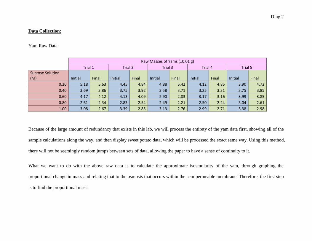
Data Collection:

Yam Raw Data:

Raw Masses of Yams (±0.01 g)

Trial 1 Trial 2 Trial 3 Trial 4 Trial 5

Sucrose Solution (M) Initial Final Initial Final Initial Final Initial Final Initial Final

0.20 5.18 5.63 4.45 4.84 4.88 5.42 4.12 4.85 3.90 4.72

0.40 3.69 3.86 3.75 3.92 3.58 3.71 3.25 3.31 3.75 3.85

0.60 4.17 4.12 4.13 4.09 2.90 2.83 3.17 3.16 3.99 3.85

0.80 2.61 2.34 2.83 2.54 2.49 2.21 2.50 2.24 3.04 2.61

1.00 3.08 2.67 3.39 2.85 3.13 2.76 2.99 2.71 3.38 2.98

Because of the large amount of redundancy that exists in this lab, we will process the entirety of the yam data first, showing all of the

sample calculations along the way, and then display sweet potato data, which will be processed the exact same way. Using this method,

there will not be seemingly random jumps between sets of data, allowing the paper to have a sense of continuity to it.

What we want to do with the above raw data is to calculate the approximate isosmolarity of the yam, through graphing the

proportional change in mass and relating that to the osmosis that occurs within the semipermeable membrane. Therefore, the first step

is to find the proportional mass.

Ding 3

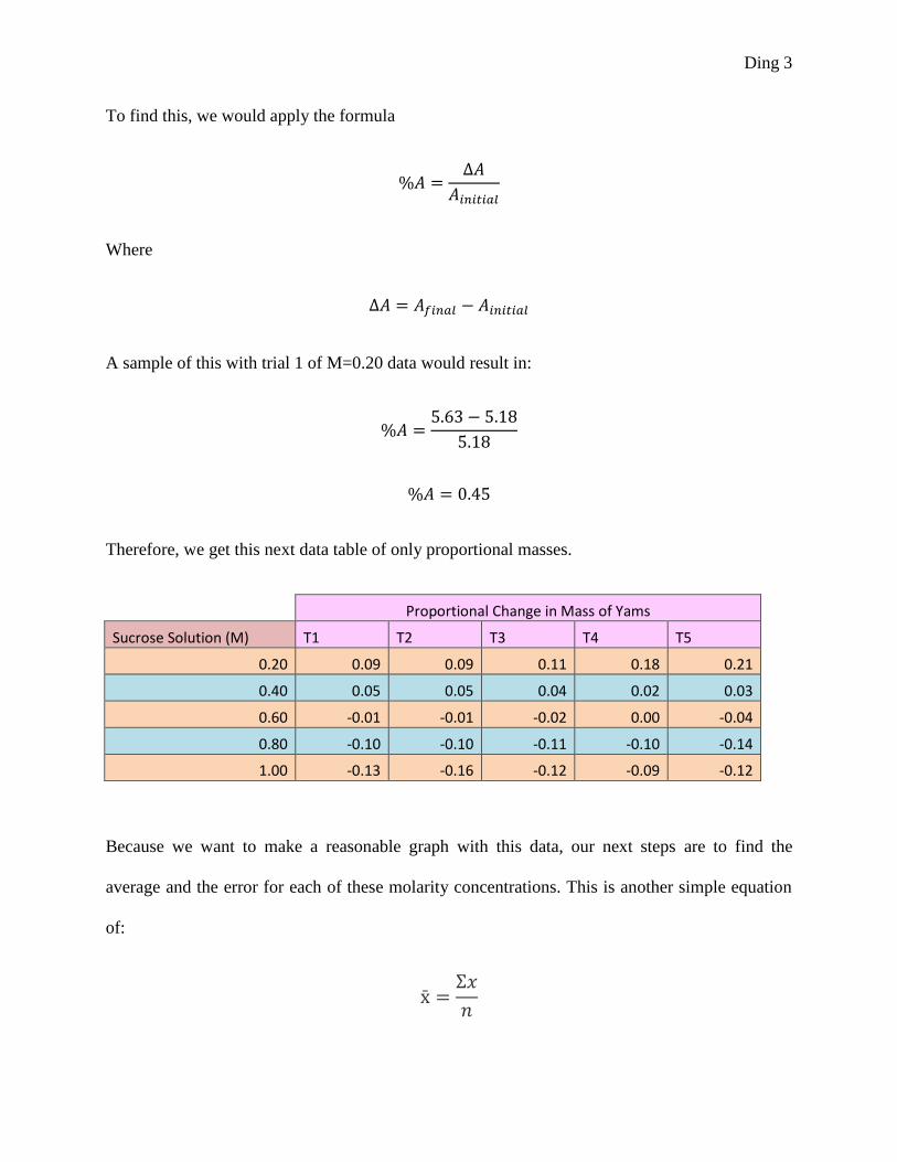
To find this, we would apply the formula

Where

A sample of this with trial 1 of M=0.20 data would result in:

Therefore, we get this next data table of only proportional masses.

Proportional Change in Mass of Yams

Sucrose Solution (M) T1 T2 T3 T4 T5

0.20 0.09 0.09 0.11 0.18 0.21

0.40 0.05 0.05 0.04 0.02 0.03

0.60 -0.01 -0.01 -0.02 0.00 -0.04

0.80 -0.10 -0.10 -0.11 -0.10 -0.14

1.00 -0.13 -0.16 -0.12 -0.09 -0.12

Because we want to make a reasonable graph with this data, our next steps are to find the

average and the error for each of these molarity concentrations. This is another simple equation

of:

Ding 4

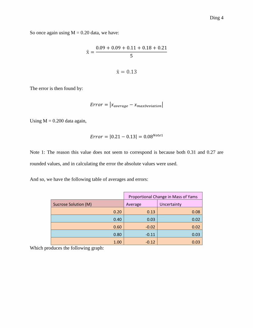
So once again using M = 0.20 data, we have:

The error is then found by:

| |

Using M = 0.200 data again,

| |

Note 1: The reason this value does not seem to correspond is because both 0.31 and 0.27 are

rounded values, and in calculating the error the absolute values were used.

And so, we have the following table of averages and errors:

Proportional Change in Mass of Yams

Sucrose Solution (M) Average Uncertainty

0.20 0.13 0.08

0.40 0.03 0.02

0.60 -0.02 0.02

0.80 -0.11 0.03

1.00 -0.12 0.03

Which produces the following graph:

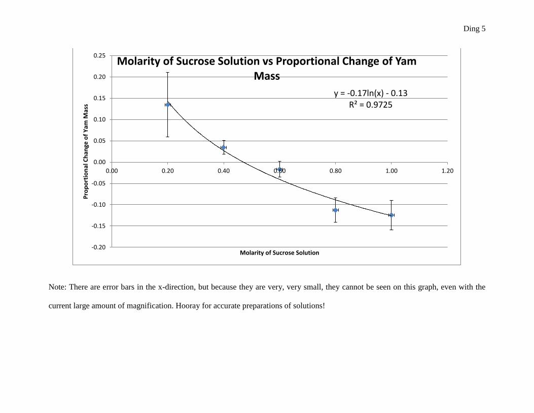
Ding 5

Note: There are error bars in the x-direction, but because they are very, very small, they cannot be seen on this graph, even with the

current large amount of magnification. Hooray for accurate preparations of solutions!

y = -0.17ln(x) - 0.13 R² = 0.9725

-0.20

-0.15

-0.10

-0.05

0.00

0.05

0.10

0.15

0.20

0.25

0.00 0.20 0.40 0.60 0.80 1.00 1.20

Pro

po

rtio

nal

Ch

ange

of

Yam

Mas

s

Molarity of Sucrose Solution

Molarity of Sucrose Solution vs Proportional Change of Yam Mass

Ding 6

The reason that I used a logarithmic graph instead of a linearized graph is this: a linear graph

does not actually make sense in biology, because it implies that as long as the sucrose solution

increase in molarity, so will the proportional change of the yam. However, due to our knowledge

of how yams are plants with plant cells, which contain a cell wall, this is not possible! If it was

an animal cell, the cell would pop at one point, but because it is a plant cell, at some point it will

become fully turgid.

As the water within the cell pushes on the cell wall, the cell wall will push back and prevent

additional water from entering the system. This type of equilibrium will eventually occur, and

thus disproves a direct linear relationship between molarity and proportional mass change.

However, because we are using a logarithmic function for regression purposes, it would be better

for us to also linearize this graph. Although we could process the isosmolarity of the x-intercept

directly from this graph, it would be better to see the linearized version in order to better

understand how well the regression fits.

In order to linearize the data, the regressed function of x will be plotted against the y value. Our

data would then require for ln(x) be plotted against the y values.

To convert into the new linearized function, we have the function:

( )

Such that for M = 0.20,

( )

Resulting in the following linearized data:

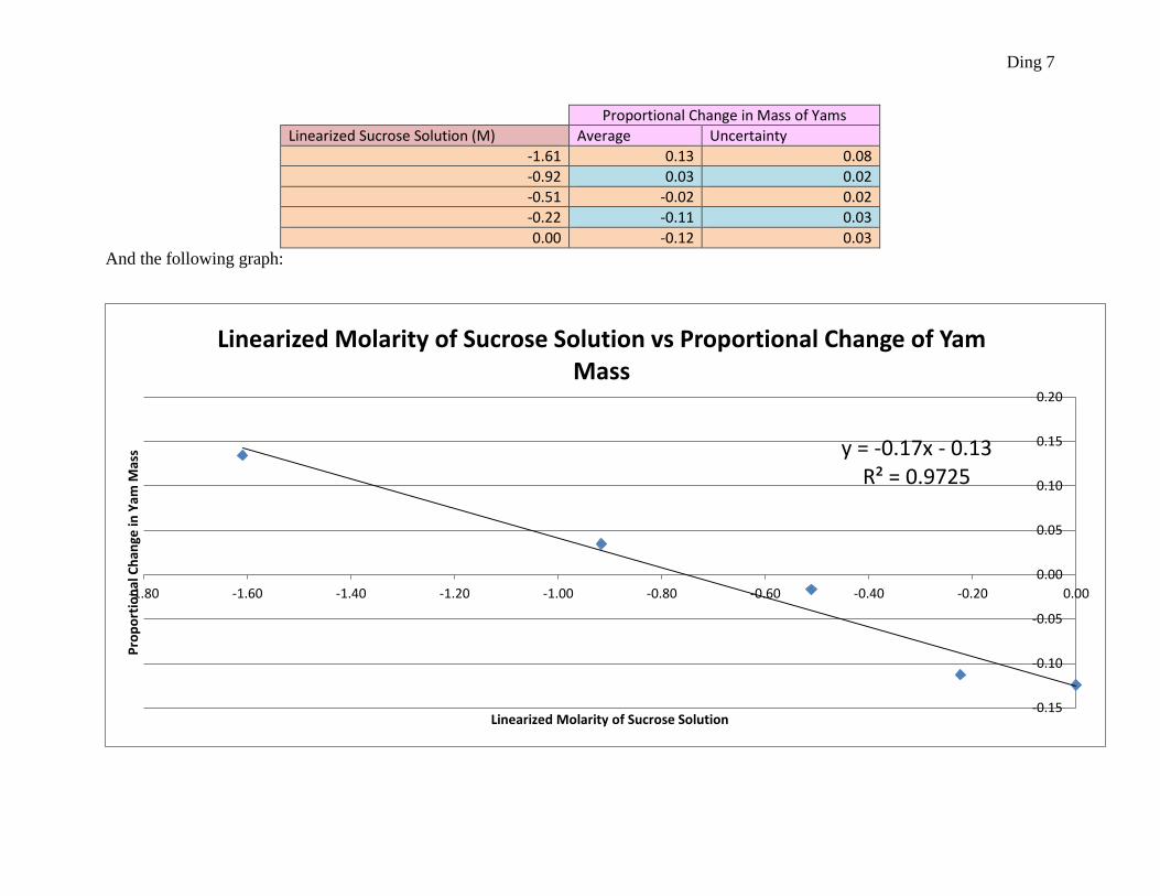
Ding 7

Proportional Change in Mass of Yams

Linearized Sucrose Solution (M) Average Uncertainty

-1.61 0.13 0.08

-0.92 0.03 0.02

-0.51 -0.02 0.02

-0.22 -0.11 0.03

0.00 -0.12 0.03

And the following graph:

y = -0.17x - 0.13 R² = 0.9725

-0.15

-0.10

-0.05

0.00

0.05

0.10

0.15

0.20

-1.80 -1.60 -1.40 -1.20 -1.00 -0.80 -0.60 -0.40 -0.20 0.00

Pro

po

rtio

nal

Ch

ange

in Y

am M

ass

Linearized Molarity of Sucrose Solution

Linearized Molarity of Sucrose Solution vs Proportional Change of Yam Mass

Ding 8

This linearized graph makes quite a bit of sense. It shows that there is a high correlation between

the data and the natural log regression, and also shows a clear intercept. Clearly, using a

logarithmic regression was a good idea.

The next step to the lab would be to calculate the x intercept. This can be done by finding the x-

intercept, or solving for x when y = 0. This results in the following formulas:

However, recall that x is actually the natural log of the concentration. Therefore, to return to the

original concentration, we must do the inverse function, or .

Therefore, the isosmotic concentration for a yam would be 0.47 M.

In order to carry out the next portion of the experiment, which is to calculate the solute potential,

it would be optimal to find the error in our value. However, this calculation is a very advanced

problem in statistical analysis. Therefore, due to limitations on time and energy, this experiment

will simply take the standard deviation of the other errors and assume that the new error is

approximately 1 standard deviation.

The formula for standard deviation is as follows:

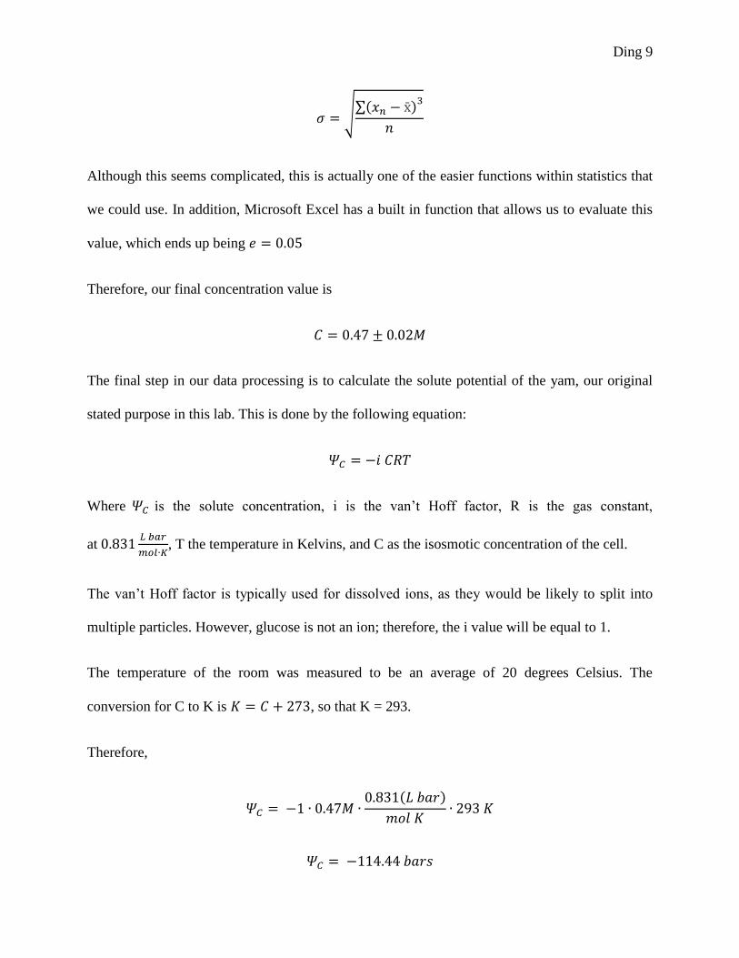
Ding 9

√∑( )

Although this seems complicated, this is actually one of the easier functions within statistics that

we could use. In addition, Microsoft Excel has a built in function that allows us to evaluate this

value, which ends up being

Therefore, our final concentration value is

The final step in our data processing is to calculate the solute potential of the yam, our original

stated purpose in this lab. This is done by the following equation:

Where is the solute concentration, i is the van’t Hoff factor, R is the gas constant,

at

, T the temperature in Kelvins, and C as the isosmotic concentration of the cell.

The van’t Hoff factor is typically used for dissolved ions, as they would be likely to split into

multiple particles. However, glucose is not an ion; therefore, the i value will be equal to 1.

The temperature of the room was measured to be an average of 20 degrees Celsius. The

conversion for C to K is , so that K = 293.

Therefore,

( )

Ding 10

In order to calculate this uncertainty, we take the percent uncertainty of the concentration and

multiply by the final value.

These equations are:

Next, we multiply by the final value to get:

So that our final answer is:

The following pages will be filled with all of the tables and graphs of the sweet potato data.

Because it is analyzed in the exact same way (and because this lab has already gone on way too

long, killing far too many trees), we will omit all of the calculations and assume that the same

procedure was followed.

Ding 11

Raw Masses of Sweet Potatoes (±0.01 g)

Trial 1 Trial 2 Trial 3 Trial 4 Trial 5

Sucrose Solution (M) Initial Final Initial Final Initial Final Initial Final Initial Final

0.20 3.33 3.86 3.30 3.70 4.21 4.66 3.73 4.30 2.63 2.97

0.40 4.04 3.84 4.20 3.48 4.27 2.81 4.07 3.35 3.45 2.71

0.60 3.42 2.60 3.29 2.48 2.86 2.26 3.12 2.35 3.31 2.73

0.80 3.48 2.18 3.99 2.58 3.63 2.88 4.66 2.39 4.21 2.92

1.00 2.74 2.20 3.16 2.19 3.00 2.21 2.94 2.17 3.72 2.56

Delta Masses of Sweet Potatoes (±0.01 g)

Sucrose Solution (M) T1 T2 T3 T4 T5

0.20 0.53 0.40 0.45 0.57 0.34

0.40 -0.2 -0.72 -1.46 -0.72 -0.74

0.60 -0.82 -0.81 -0.60 -0.77 -0.58

0.80 -1.3 -1.41 -0.75 -2.27 -1.29

1.00 -0.54 -0.97 -0.79 -0.77 -1.16

Proportional Change in Mass in Sweet Potatoes

Sucrose Solution (M) T1 T2 T3 T4 T5

0.20 0.16 0.12 0.11 0.15 0.13

0.40 -0.05 -0.17 -0.34 -0.18 -0.21

0.60 -0.24 -0.25 -0.21 -0.25 -0.18

0.80 -0.37 -0.35 -0.21 -0.49 -0.31

1.00 -0.20 -0.31 -0.26 -0.26 -0.31

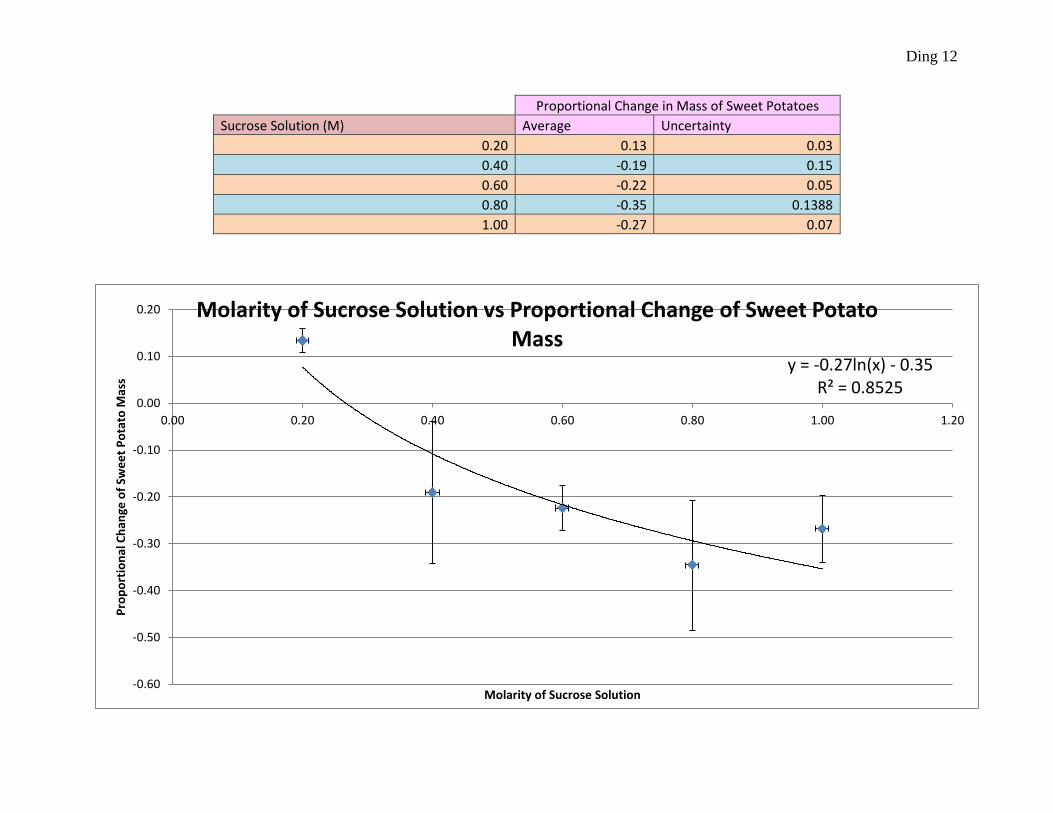
Ding 12

Proportional Change in Mass of Sweet Potatoes

Sucrose Solution (M) Average Uncertainty

0.20 0.13 0.03

0.40 -0.19 0.15

0.60 -0.22 0.05

0.80 -0.35 0.1388

1.00 -0.27 0.07

y = -0.27ln(x) - 0.35 R² = 0.8525

-0.60

-0.50

-0.40

-0.30

-0.20

-0.10

0.00

0.10

0.20

0.00 0.20 0.40 0.60 0.80 1.00 1.20

Pro

po

rtio

nal

Ch

ange

of

Swe

et

Po

tato

Mas

s

Molarity of Sucrose Solution

Molarity of Sucrose Solution vs Proportional Change of Sweet Potato Mass

Ding 13

Proportional Change in Mass of Sweet Potatoes

Linearized Sucrose Solution (M) Average Uncertainty

-1.61 0.13 0.03

-0.92 -0.19 0.15

-0.51 -0.22 0.05

-0.22 -0.35 0.1388

0.00 -0.27 0.07

y = -0.27x - 0.35 R² = 0.8525

-0.40

-0.30

-0.20

-0.10

0.00

0.10

0.20

-1.80 -1.60 -1.40 -1.20 -1.00 -0.80 -0.60 -0.40 -0.20 0.00

Pro

po

rtio

nal

Ch

ange

in S

we

et

Po

tato

Mas

s

Linearized Molarity of Sucrose Solution

Linearized Molarity of Sucrose Solution vs Proportional Change of Sweet Potato Mass

Ding 14

( )

Conclusion:

This was a very interesting lab that explored the osmotic potential of different vegetables such as

the sweet potato and the yam. Through experimentation, we determined the concentration of a

yam and a sweet potato, and then proceeded to calculate the osmotic potential based on these

numbers. Because our lab was structured more around a “find the value” lab rather than an

inquiry lab, there is no true “validation” of a theory or hypothesis that we can do here. However,

it is interesting to note what a large difference exists between yams and sweet potatoes!

After completing the entire lab, we have shown that while yams have a solute potential of -114

bars, sweet potatoes have a much higher solute potential, at -65.74 bars. This allows us to

conclude about the various differences between composition of a sweet potato versus a yam,

despite their similar appearances and use in dishes. It most likely points to a different glucose or

starch concentration within either one of them. Because solute potential should decrease with

higher concentrations, it implies that yams have much more sugar in them than “sweet” potatoes.

Ding 15

One additional case to note is the justification for the logarithmic fit for the regression lines.

Similar to the paper published concerning gummy bear concentrations by Ding. C and Ding. S,

the logarithmic fit was clearly better at modeling the function than any other function. Therefore,

we have outside validation that the methods we used in this lab were accurate.

However, there are several errors in this lab. For one, the experimenters would like to declare

that this was not a single-person lab, but instead, a group collaboration by Mr. Allen’s 3rd

period

AP/IB Biology class. Therefore, the data for each varying molarity of sucrose solution was

collected by a different individual. This results in a non-controlled experimenter, which may

have led to data-recording errors and, in general, non-homogenous procedures.

Although the fix for this error is simple, to have one person carry out all of the experiments, this

is not necessarily practical, due to the very large data set that is required. Therefore, a better

improvement would be to have different people doing different molarities. Therefore, if person A

used to do all 5 trials of M = 0.20, s/he would now do 1 trial each of M = 0.20, 0.40, 0.60, 0.80,

1.00. Therefore, errors made in the process would be better caught and averaged out by the group.

Of course, increasing the number of experimenters would actually set up for more statistically-

accurate data.

Another error was in the way that the vegetable pieces were chopped up. This human error was

due to the difficulty in chopping an exact 1cubic centimeter piece of vegetable using nothing but

a dull knife and a ruler. Therefore, many of the “cubes” had lopsided faces or deviated by as

much as half a centimeter. This may have led to a large discrepancy between groups, as well as

for the experiment as a whole.

Ding 16

A solution to this would be to use some sort of cutting tool, perhaps an iron grid with pre-made

spacings of 1 cm squares and slice the vegetables. This would guarantee uniform strands,

eliminating the sloppy cutting of high school students.

One final random error is in the way that nature creates sweet potatoes and yams. Nature is not a

factory; while the basic DNA is the same, each potato has slight variations, and thus different

molarities and osmotic potentials. However, through our statistical averaging, we can assume

that we eliminate the randomness and have found an average for each vegetable.

Unfortunately, in conclusion, there is published data by the United States Department of

Agriculture that reveals that while yams have a combined starch and fiber content of 4.6 grams

per 100 grams of yam, sweet potatoes have a whopping 7.18 grams per 100 grams of sweet

potato, almost double that of yams and casting the conclusions found in this lab into serious

doubt. However, the experimenter would like to note that there is a vast amount of confusion

between what is a “sweet potato” and what is a “yam”. While in the US, both terms are often

used to refer to an edible tuberous root that is long and tapered, with colors of orange, red, or

yellow, a true yam is longer and harder than a sweet potato, and is much more starchier. Yams

are most often found in Western Africa, where it is a precious commodity (See: Things Fall

Apart).

Therefore, what we have really shown is that there are lots of differences between the way that

each kind of plant grows. Depending on the genes within that plant, the sugar and starch contents

can vary by a very large amount.

Ding 17

Works Cited

Achebe, Chinua. Things Fall Apart. New York: Anchor, 1994. Print.

Ding, Chunyang, and Siyao Ding. "Gummy Bear Lab." Allen Biology 3rd 1.1 (2013): 1-6. Print.

"Nutrient data laboratory". United States Department of Agriculture. Retrieved January 2012.