X3D: Expanding Architectures for Efficient Video Recognition

Christoph Feichtenhofer

Facebook AI Research (FAIR)

Abstract

This paper presents X3D, a family of efficient video net-works that progressively expand a tiny 2D image classifi-cation architecture along multiple network axes, in space,time, width and depth. Inspired by feature selection methodsin machine learning, a simple stepwise network expansionapproach is employed that expands a single axis in each step,such that good accuracy to complexity trade-off is achieved.To expand X3D to a specific target complexity, we performprogressive forward expansion followed by backward con-traction. X3D achieves state-of-the-art performance whilerequiring 4.8× and 5.5× fewer multiply-adds and parame-ters for similar accuracy as previous work. Our most surpris-ing finding is that networks with high spatiotemporal resolu-tion can perform well, while being extremely light in terms ofnetwork width and parameters. We report competitive accu-racy at unprecedented efficiency on video classification anddetection benchmarks. Code will be available at: https://github.com/facebookresearch/SlowFast.

1. IntroductionNeural networks for video recognition have been largely

driven by expanding 2D image architectures [29, 47, 64, 71]into spacetime. Naturally, these expansions often happenalong the temporal axis, involving extending the networkinputs, features, and/or filter kernels into spacetime (e.g.[7, 13, 17, 42, 56, 75]); other design decisions—includingdepth (number of layers), width (number of channels), andspatial sizes—however, are typically inherited from 2D im-age architectures. While expanding along the temporal axis(while keeping other design properties) generally increasesaccuracy, it can be sub-optimal if one takes into account thecomputation/accuracy trade-off —a consideration of centralimportance in applications.

In part because of the direct extension of 2D modelsto 3D, video recognition architectures are computationallyheavy. In comparison to image recognition, typical videomodels are significantly more compute-demanding, e.g. animage ResNet [29] can use around 27× fewer multiply-addoperations than a temporally extended video variant [81].

T

C

H,W

prediction

Ít

ÍÜÍs

Íd

Íw

Íb

Ís

Input framesres2 res3

res4

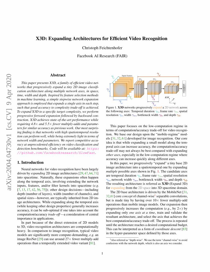
Figure 1. X3D networks progressively expand a 2D network acrossthe following axes: Temporal duration γt, frame rate γτ , spatialresolution γs, width γw, bottleneck width γb, and depth γd.

This paper focuses on the low-computation regime interms of computation/accuracy trade-off for video recogni-tion. We base our design upon the “mobile-regime" mod-els [31, 32, 61] developed for image recognition. Our coreidea is that while expanding a small model along the tem-poral axis can increase accuracy, the computation/accuracytrade-off may not always be best compared with expandingother axes, especially in the low-computation regime whereaccuracy can increase quickly along different axes.

In this paper, we progressively “expand" a tiny base 2Dimage architecture into a spatiotemporal one by expandingmultiple possible axes shown in Fig. 1. The candidate axesare temporal duration γt, frame rate γτ , spatial resolutionγs, network width γw, bottleneck width γb, and depth γd.The resulting architecture is referred as X3D (Expand 3D)for expanding from the 2D space into 3D spacetime domain.

The 2D base architecture is driven by the MobileNet [31,32,61] core concept of channel-wise1 separable convolutions,but is made tiny by having over 10× fewer multiply-addoperations than mobile image models. Our expansion thenprogressively increases the computation (e.g., by 2×) byexpanding only one axis at a time, train and validate theresultant architecture, and select the axis that achieves thebest computation/accuracy trade-off. The process is repeateduntil the architecture reaches a desired computational budget.This can be interpreted as a form of coordinate descent [83]in the hyper-parameter space defined by those axes.

1Also referred as “depth-wise". We use the term “channel-wise" to avoidconfusions with the network depth, which is also an axis we consider.

1

arX

iv:2

004.

0473

0v1

[cs

.CV

] 9

Apr

202

0

Our progressive network expansion approach is inspiredby the history of image ConvNet design where popu-lar architectures have arisen by expansions across depth,[8,29,47,64,71,94], resolution [35,70,73] or width [88,93],and classical feature selection methods [25, 41, 44] in ma-chine learning. In the latter, progressive feature selectionmethods [25, 44] start with either a set of minimum featuresand aim to find relevant features to improve in a greedy fash-ion by including (forward selection) a single feature in eachstep, or start with a full set of features and aim to find irrele-vant ones that are excluded by repeatedly deleting the featurethat reduces performance the least (backward elimination).

To compare to previous research, we use Kinetics-400[43], Kinetics-600 [4], Charades [62] and AVA [24]. Forsystematic studies, we classify our models into differentlevels of complexity for small, medium and large models.

Overall, our expansion produces a sequence of spatiotem-poral architectures, covering a wide range of computa-tion/accuracy trade-offs. They can be used under differ-ent computational budgets that are application-dependentin practice. For example, across different computation andaccuracy regimes X3D performs favorably to state-of-the-art while requiring 4.8× and 5.5× fewer multiply-adds andparameters for similar accuracy as previous work. Further,expansion is simple and cheap e.g. our low-compute modelis completed after only training 30 tiny models that accumu-latively require over 25× fewer multiply-add operations fortraining than one large state-of-the-art network [15, 81, 84].

Conceptually, our most surprising finding is that verythin video architectures that are created by expanding spatio-temporal resolution perform well, while being light in termsof network width and parameters. X3D networks have lowerwidth than image-design [29, 64, 71] based video models,making X3D similar to the high-resolution Fast pathway [15]which has been designed in such fashion. We hope theseadvances will facilitate future research and applications.

2. Related WorkSpatiotemporal (3D) networks. Video recognition archi-tectures are favorably designed by extending image classifi-cation networks with a temporal dimension, and preservingthe spatial properties. These extensions include direct trans-formation of 2D models [29, 47, 64, 71] such as ResNet orInception to 3D [7, 26, 58, 74, 75, 89], adding RNNs on topof 2D CNNs [13, 49, 50, 56, 67, 92], or extending 2D modelswith an optical flow stream that is processed by an identical2D network [7, 18, 63, 80] . While starting with a 2D imagebased model and converting it to a spatiotemporal equivalentby inflating filters [7, 17] allows pretraining on image classi-fication tasks, it makes video architectures inherently biasedtowards their image-based counterparts.

The SlowFast [15] architecture has explored the resolu-tion trade-off across several axes, different temporal, spatial,

and channel resolution in the Slow and Fast pathway. Inter-estingly the Fast pathway can be very thin and therefore onlyadds a small computational overhead; however, performs lowin isolation. Further, these explorations were performed withthe architecture of the computationally heavy Slow pathwayheld constant to a temporal extension of an image classifica-tion design [29]. In relation to this previous effort, our workinvestigates whether the heavy Slow pathway is required, orif a lightweight network can be made competitive.

Efficient 2D networks. Computation-efficient architec-tures have been extensively developed for the image clas-sification task, with MobileNetV1&2 [32, 61] and Shuf-fleNet [95] exploring channel-wise separable convolutionsand expanded bottlenecks. Several methods for neural archi-tecture search in this setting have been proposed, also addingSqueeze-Excitation (SE) [33] attention blocks to the designspace in [72] and more recently, MobileNetV3 [31] Swishnon-linearities [59]. MobileNets [32, 61, 72] were scaledup and down by using a multiplier for width and input size(resolution). Recently, MnasNet [72] is used to apply linerscaling factors to spatial, width and depth axes for creating aset of EfficientNets [73] for image classification.

Our expansion is related to this, but requires fewer sam-ples and handles more axes as we only train a single modelfor each axis in each step, while [73] performs a grid-searchon the initial regime which requires kd models to be trainedwhere k is the gridsize and d the number of axes. Moreover,the model used for this search, MnasNet was found by sam-pling around 8000 models [72]. For video, this is prohibitiveas datasets can have orders of magnitude more images thanimage classification e.g. the largest version of Kinetics [5]has ≈195M frames, 162.5× more images than ImageNet.By contrast, our approach only requires to train 6 models,one for each expansion axis, until a desired complexity isreached, e.g. for 5 steps, it requires 30 models to be trained.

Efficient 3D networks. Several innovative architectures forefficient video classification have been proposed, e.g. [3, 6,10,12,14,19,36,45,48,55,57,68,69,76,78,79,85,89,97–99].Channel-wise separable convolution as a key building blockfor efficient 2D ConvNets [31, 32, 61, 73, 95] has been ex-plored for video classification in [45,76], where 2D architec-tures are extended to their 3D counterparts, e.g. ShuffleNetand MobileNet in [45], or ResNet in [76] by using a 3×3×3channel-wise separable convolution in the bottleneck of aresidual stage. Earlier, [10] adopt 2D ResNets and Mo-bileNets from ImageNet and sparsifies connections insideeach residual block similar to separable or group convolu-tion. A temporal shift module (TSM) is introduced in [51]that extends a ResNet to capture temporal information usingmemory shifting operations. There is also active research onadaptive frame sampling techniques, e.g. [2,46,65,86,87,91],which we think can be complementary to our approach.

2

In relation to most of these works, our approach doesnot assume a fixed inherited design from 2D networks, butexpands a tiny architecture across several axes in space, time,channels and depth to achieve a good efficiency trade-off.

3. X3D NetworksImage classification architectures have gone through an

evolution of architecture design with progressively expand-ing existing models along network depth [8,29,47,64,71,94],input resolution [35, 70, 73] or channel width [88, 93]. Simi-lar progress can be observed for the mobile image classifi-cation domain where contracting modifications (shallowernetworks, lower resolution, thinner layers, separable convo-lution [31, 32, 37, 61, 95]) allowed operating at lower compu-tational budget. Given this history in image ConvNet design,a similar progress has not been observed for video architec-tures as these were customarily based on direct temporalextensions of image models. However, is single expansionof a fixed 2D architecture to 3D ideal, or is it better to expandor contract along different axes?

For video classification the temporal dimension exposesan additional dilemma, increasing the number of possibilitiesbut also requiring it to be dealt differently than the spatialdimensions [15, 63, 77]. We are especially interested in thetrade-off between different axes, more concretely:

• What is the best temporal sampling strategy for 3Dnetworks? Is a long input duration and sparser samplingpreferred over faster sampling of short duration clips?

• Do we require finer spatial resolution? Previous workshave used lower resolution for video classification[42, 75, 77] to increase efficiency. Also, videos typi-cally come at coarser spatial resolution than Internetimages; therefore, is there a maximum spatial resolu-tion at which performance saturates?

• Is it better to have a network with high frame-rate butthinner channel resolution, or to slowly process videowith a wider model? E.g. should the network haveheavier layers as typical image classification models(and the Slow pathway [15]) or rather lighter layerswith lower width (as the Fast pathway [15]). Or is therea better trade-off, possibly between these extremes?

• When increasing the network width, is it better to glob-ally expand the network width in the ResNet blockdesign [29] or to expand the inner (“bottleneck”) width,as is common in mobile image classification networksusing channel-wise separable convolutions [61, 95]?

• Should going deeper be performed with expanding in-put resolution in order to keep the receptive field sizelarge enough and its growth rate roughly constant, or isit better to expand into different axes? Does this holdfor both the spatial and temporal dimension?

stage filters output sizes T×S2

data layer stride γτ , 12 1γt×(112γs)2

conv1 1×32, 3×1, 24γw 1γt×(56γs)2

res2

1×12, 24γbγw3×32, 24γbγw

1×12, 24γw

×γd 1γt×(28γs)2

res3

1×12, 48γbγw3×32, 48γbγw

1×12, 48γw

×2γd 1γt×(14γs)2

res4

1×12, 96γbγw3×32, 96γbγw

1×12, 96γw

×5γd 1γt×(7γs)2

res5

1×12, 192γbγw3×32, 192γbγw

1×12, 192γw

×3γd 1γt×(4γs)2

conv5 1×12, 192γbγw 1γt×(4γs)2

pool5 1γt×(4γs)2 1×1×1fc1 1×12, 2048 1×1×1fc2 1×12, #classes 1×1×1

Table 1. X3D architecture. The dimensions of kernels are denotedby {T×S2, C} for temporal, spatial, and channel sizes. Stridesare denoted as {temporal stride, spatial stride2}. This network isexpanded using factors {γτ , γt, γs, γw, γb, γd} to form X3D.Without expansion (all factors equal to one), this model is referredto as X2D, having 20.67M FLOPS and 1.63M parameters.

This section first introduces the basis X2D architecturein Sec. 3.1 which is expanded with operations defined inSec. 3.2 by using the progressive approach in Sec. 3.3.

3.1. Basis instantiation

We begin by describing the instantiation of the basisnetwork architecture, X2D, that serves as baseline to beexpanded into spacetime. The basis network instantiationfollows a ResNet [29] structure and the Fast pathway designof SlowFast networks [15] with degenerated (single frame)temporal input. X2D is specified in Table 1, if all expansionfactors {γτ , γt, γs, γw, γb, γd} are set to 1.

We denote spatiotemporal size by T×S2 where T is thetemporal length and S is the height and width of a squarespatial crop. The X2D architecture is described next.

Network resolution and channel capacity. The modeltakes as input a raw video clip that is sampled with frame-rate 1/γτ in the data layer stage. The basis architecture onlytakes a single frame of size T×S2=1×1122 as input andtherefore can be seen as an image classification network.The width of the individual layers is oriented at the Fastpathway design in [15] with the first stage, conv1, filtersthe 3 RGB input channels and produces 24 output features.This width is increased by a factor of 2 after every spatialsub-sampling with a stride = 1, 22 at each deeper stage fromres2 to res5. Spatial sub-sampling is performed by the center(“bottleneck”) filter of the first res-block of each stage.

3

Similar to the SlowFast pathways [15], the model pre-serves the temporal input resolution for all features through-out the network hierarchy. There is no temporal downsam-pling layer (neither temporal pooling nor time-strided con-volutions) throughout the network, up to the global poolinglayer before classification. Thus, the activations tensors con-tain all frames along the temporal dimension, maintainingfull temporal frequency in all features.

Network stages. X2D consists of a stage-level and bottle-neck design that is inspired by recent 2D mobile image clas-sification networks [31, 32, 61, 95] which employ channel-wise separable convolution that are a key building blockfor efficient ConvNet models. We adopt stages that followMobileNet [31, 61] design by extending every spatial 3×3convolution in the bottleneck block to a 3×3×3 (i.e. 3×32)spatiotemporal convolution which has also been explored forvideo classification in [45, 76]. Further, the 3×1 temporalconvolution in the first conv1 stage is channel-wise.

Discussion. X2D can be interpreted as a Slow pathwaysince it only uses a single frame as input, while the networkwidth is similar to the Fast pathway in [15] which is muchlighter than typical 3D ConvNets (e.g., [7, 15, 17, 75, 81])that follow an ImageNet design. Concretely, it only requires20.67M FLOPs which amounts to only 0.0097% of a recentstate-of-the-art SlowFast network [15].

As shown in Table 1 and Fig. 1, X2D is expanded across6 axes, {γτ , γt, γs, γw, γb, γd}, described next.

3.2. Expansion operations

We define a basic set of expansion operations that areused for sequentially expanding X2D from a tiny spatialnetwork to X3D, a spatiotemporal network, by performingthe following operations on temporal, spatial, width anddepth dimensions.

• X-Fast expands the temporal activation size, γt, byincreasing the frame-rate, 1/γτ , and therefore temporalresolution, while holding the clip duration constant.

• X-Temporal expands the temporal size, γt, by samplinga longer temporal clip and increasing the frame-rate1/γτ , to expand both duration and temporal resolution.

• X-Spatial expands the spatial resolution, γs, by increas-ing the spatial sampling resolution of the input video.

• X-Depth expands the depth of the network by increas-ing the number of layers per residual stage by γd times.

• X-Width uniformly expands the channel number for alllayers by a global width expansion factor γw.

• X-Bottleneck expands the inner channel width, γb, ofthe center convolutional filter in each residual block.

3.3. Progressive Network Expansion

We employ a simple progressive algorithm for networkexpansion, similar to forward and backward algorithms forfeature selection [25, 39, 41, 44]. Initially we start with X2D,the basis model instantiation with a set of unit expandingfactors X0 of cardinality a. We use a = 6 factors, X ={γτ ,γt, γs, γw, γb, γd}, but other axes are possible.

Forward expansion. The network expansion criterion func-tion, which measures the goodness for the current expansionfactors X , is represented as J(X ). Higher scores of this mea-sure represent better expanding factors, while lower scoreswould represent worse. In our experiments, this correspondsto the accuracy of a model expanded by X . Furthermore, letC(X ) be a complexity criterion function that measures thecost of the current expanding factors X . In our experiments,C is set to the floating point operations of the underlyingnetwork instantiation expanded by X , but other measuressuch as runtime, parameters, or memory are possible. Then,the network expansion tries to find expansion factors X withthe best trade-off X = argmaxZ,C(Z)=c = J(Z) where Zare the possible expansion factors to be explored and c isthe target complexity. In our case we perform expansionthat only changes a single one of the a expansion factorswhile holding the others constant; therefore there are only adifferent subsets of Z to evaluate, where each of them altersin only one dimension from X . The expansion with the bestcomputation/accuracy trade-off is kept for the next step. Thisis a form of coordinate descent [83] in the hyper-parameterspace defined by those axes.

The expansion is performed in a progressive manner withan expansion-rate c that corresponds to the stepsize at whichthe model complexity c is increased in each expansion step.We use a multiplicative increase of c ≈ 2 of the modelcomplexity in each step that corresponds to the complexity-increase for doubling the number of frames of the model.The stepwise expansion is therefore simple and efficient as itonly requires to train a few models until a target complexityis reached, since we exponentially increase the complexity.Details on the expansion are in §A.3.

Backward contraction. Since the forward expansion onlyproduces models in discrete steps, we perform a backwardcontraction step to meet a desired target complexity, if thetarget is exceeded by the forward expansion steps. Thiscontraction is implemented as a simple reduction of the lastexpansion, such that it matches the target. For example, ifthe last step has increased the frame-rate by a factor of two,the backward contraction will reduce the frame-rate by afactor < 2 to roughtly match the desired target complexity.

4. Experiments: Action ClassificationDatasets. We perform our expansion on Kinetics-400 [43](K400) with ∼240k training, 20k validation and 35k testing

4

τ

sd

b

t

w

X3D

d

d

t

t

b

τ

τ

X3D-LX3D-MX3D-S

X3D-XS

s

ss

X2D

wX3D-XL

Model capacity in GFLOPs (# of multiply-adds x 109)0 5 15 25 3510 20 30

80

75

70

65

60

55

50

Kin

etic

s to

p-1

accu

racy

(%)

Figure 2. Progressive network expansion of X3D. The X2D basemodel is expanded 1st across bottleneck width (γb), 2nd tempo-ral resolution (γτ ), 3rd spatial resolution (γs), 4th depth (γd), 5th

duration (γt), etc. The majority of models are trained for smallcomputation cost, making the expansion economical in practice.

videos in 400 human action categories. We report top-1and top-5 classification accuracy (%). As in previous work,we train and report ablations on the train and val sets. Wealso report results on test set as the labels have been madeavailable [4]. We report the computational cost (in FLOPs)of a single, spatially center-cropped clip.2

Training. All models are trained from random initialization(“from scratch”) on Kinetics, without using ImageNet [11]or other pre-training. Our training recipe follows [15]. Allimplementation details and dataset specifics are in §A.3.

For the temporal domain, we randomly sample a clipfrom the full-length video, and the input to the networkare γt frames with a temporal stride of γτ ; for the spatialdomain, we randomly crop 112γs×112γs pixels from avideo, or its horizontal flip, with a shorter side randomlysampled in [128γs, 160γs] pixels which is a linearly scaledversion of the augmentation used in [15, 64, 81].

Inference. To be comparable with previous work and eval-uate accuracy/complexity trade-offs we apply two test-ing strategies: (i) K-Center: Temporally, uniformly sam-ples K clips (e.g. K=10) from a video and spatiallyscales the shorter spatial side to 128γs pixels and takesa γt×112γs×112γs center crop, comparable to [46, 51, 76,84]. (ii) K-LeftCenterRight is the same as above temporally,but takes 3 crops of γt×128γs×128γs to cover the longerspatial axis, as an approximation of fully-convolutional test-ing, following [15, 81]. We average the softmax scores forall individual predictions.

2We use single-clip, center-crop FLOPs as a basic unit of computationalcost. Inference-time computational cost is roughly proportional to this, if afixed number of clips and crops is used, as is for our all models.

model top-1 top-5regime FLOPs ParamsFLOPs (G) (G) (M)

X3D-XS 68.6 87.9 X-Small ≤ 0.6 0.60 3.76X3D-S 72.9 90.5 Small ≤ 2 1.96 3.76X3D-M 74.6 91.7 Medium ≤ 5 4.73 3.76X3D-L 76.8 92.5 Large ≤ 20 18.37 6.08X3D-XL 78.4 93.6 X-Large ≤ 40 35.84 11.0X3D-XXL 80.0 94.5 XX-Large ≤ 150 143.5 20.3

Table 2. Expanded instances on K400-val. 10-Center clip testing isused. We show top-1 and top-5 classification accuracy (%), as wellas computational complexity measured in GFLOPs (floating-pointoperations, in # of multiply-adds ×109) for a single clip input.Inference-time computational cost is proportional to 10× of this,as a fixed number of 10 of clips is used per video.

4.1. Expanded networks

The accuracy/complexity trade-off curve for the expan-sion process on K400 is shown in Fig. 2. Expansion startsfrom X2D that produces 47.75% top-1 accuracy (verticalaxis) with 1.63M parameters 20.67M FLOPs per clip (hori-zontal axis), which is roughly doubled in each progressivestep. We use 10-Center clip testing as our default test settingfor expansion, so the overall cost per video is ×10. Wewill ablate different number of testing clips in Sec. 4.3. Theexpansion in Fig. 2 provides several interesting observations:

(i) First of all, expanding along any one of the candidateaxes increases accuracy. This justifies our motivation oftaking multiple axes (instead of just the temporal axis) intoaccount when designing spatiotemporal models.

(ii) Surprisingly, the first step selected by the expansionalgorithm is not along the temporal axis; instead, it is a factorthat grows the “bottleneck" width γb in the ResNet blockdesign [29]. This echoes the inverted bottleneck designin [61] (called “inverted residual" [61]). This is possiblybecause these layers are lightweight (due to the channel-wisedesign of MobileNets) and thus are economical to expand atfirst. Another interesting observation is that accuracy variesstrongly, with the bottleneck expansion γb providing thehighest top-1 accuracy of 55.0% and depth expansion γd thelowest with 51.3% at same complexity of 41.4M FLOPs.

(iii) The second step extends the temporal size of themodel from one to two frames (expanding γτ and γt isidentical for this step as there exists only a single frame inthe previous one). This is what we expected to be the mosteffective expansion already in the first step as it enables thenetwork to model temporal information for recognition.

(iv) The third step increases the spatial resolution γs andstarts to show a pattern that is interesting. The expansionincreases spatial and temporal resolution followed by depth(γd) in the fourth step. This is followed by multiple temporalexpansions that increase temporal resolution (i.e. frame-rate)and input duration (γτ & γt), followed by two more expan-sions across the spatial resolution, γs, in steps 8 and 9, whilestep 10 increases the depth of the network, γd. An expansionof the depth after increasing input resolution is intuitive, asit allows to grow the filter receptive field resolution and sizewithin each residual stage.

5

stage filters output sizes T×H×Wdata layer stride 6, 12 13×160×160

conv1 1×32, 3×1, 24 13×80×80

res2

1×12, 543×32, 541×12, 24

×3 13×40×40

res3

1×12, 1083×32, 1081×12, 48

×5 13×20×20

res4

1×12, 2163×32, 2161×12, 96

×11 13×10×10

res5

1×12, 4323×32, 4321×12, 192

×7 13×5×5

conv5 1×12, 432 13×5×5pool5 13×5×5 1×1×1

fc1 1×12, 2048 1×1×1fc2 1×12, #classes 1×1×1

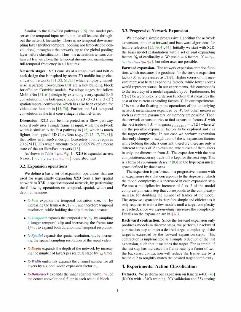
(a) X3D-S with 1.96G FLOPs, 3.76M param, and72.9% top-1 accuracy using expansion of γτ= 6,γt= 13, γs=

√2, γw= 1, γb= 2.25, γd= 2.2.

stage filters output sizes T×H×Wdata layer stride 5, 12 16×224×224

conv1 1×32, 3×1, 24 16×112×112

res2

1×12, 543×32, 541×12, 24

×3 16×56×56

res3

1×12, 1083×32, 1081×12, 48

×5 16×28×28

res4

1×12, 2163×32, 2161×12, 96

×11 16×14×14

res5

1×12, 4323×32, 4321×12, 192

×7 16×7×7

conv5 1×12, 432 16×7×7pool5 16×7×7 1×1×1

fc1 1×12, 2048 1×1×1fc2 1×12, #classes 1×1×1

(b) X3D-M with 4.73G FLOPs, 3.76M param, and74.6% top-1 accuracy using expansion of γτ= 5,γt= 16, γs= 2, γw= 1, γb= 2.25, γd= 2.2.

stage filters output sizes T×H×Wdata layer stride 5, 12 16×312×312

conv1 1×32, 3×1, 32 16×156×156

res2

1×12, 723×32, 721×12, 32

×5 16×78×78

res3

1×12, 1623×32, 1621×12, 72

×10 16×39×39

res4

1×12, 3063×32, 3061×12, 136

×25 16×20×20

res5

1×12, 6303×32, 6301×12, 280

×15 16×10×10

conv5 1×12, 630 16×10×10pool5 16×10×10 1×1×1

fc1 1×12, 2048 1×1×1fc2 1×12, #classes 1×1×1

(c) X3D-XL with 35.84G FLOPs & 10.99M param,and 78.4% top-1 acc. using expansion of γτ= 5,γt= 16, γs= 2

√2, γw= 2.9, γb= 2.25, γd= 5.

Table 3. Three instantiations of X3D with varying complexity. The top-1 accuracy corresponds to 10-Center view testing on K400. Themodels in (a) and (b) only differ in spatiotemporal resolution of the input and activations (γt, γτ , γs), and (c) differs from (b) in spatialresolution, γs, width, γw, and depth, γd. See Table 1 for X2D. Surprisingly X3D-XL has a maximum width of 630 feature channels.

(v) Even though we start from a base model that is in-tentionally made tiny by having very few channels, the ex-pansion does not choose to globally expand the width up tothe 10th step of the expansion process, making X3D similarto the Fast pathway design [16] with high spatiotemporalresolution but low width. The last expansion step shown inthe top-right of Fig. 2 increases the width γw. The final twosteps, not shown in Fig. 2, expand γτ and γd.

In the spirit of VGG models [8, 64] we define a set ofnetworks based on their target complexity. We use FLOPs asthis reflects a hardware agnostic measure of model complex-ity. Parameters are also possible, but as they would not besensitive to the input and activation tensor size, we only re-port them as secondary metric. To cover the models from ourexpansion, Table 2 defines complexity regimes by FLOPs,ranging from extra small (XS) to extra extra large (XXL).

Expanded instances. The smallest instance, X3D-XS isthe output after 5 expansion steps. Expansion is simple andefficient as it requires to train few models that are mostly ata low compute regime. For X3D-XS each step trains modelsof around 0.04, 0.08, 0.15, 0.30, 0.60 GFLOPs. Since wetrain one model for each of the 6 axes the approximate costfor these five steps is roughly equal to training a single modelof 6 ×1.17 GFLOPS (to be fair, this ignores overhead costfor data loading etc. as 6×5=30 models are trained overall).

The next larger model is X3D-S which is defined by onebackward contraction step after the 7th expansion step. Thecontraction step simply reduces the expansion (γt) propor-tionally to roughly match the target regime of ≤ 2 GFLOPs.For this model we also tried to contract each other axis tomatch the target and found that γt is best among the others.

The next models in Table 2 is X3D-M (≤ 2 GFLOPs)that achieves 74.6% top-1 accuracy, X3D-L (≤ 20 GFLOPs)with 76.8% top-1 and X3D-XL (≤ 40 GFLOPs) with 78.4%and X3D-XXL (≤ 150 GFLOPs) with 80.0% top-1 accuracy

by expansion in the consecutive steps.Further speed/accuracy comparisons are provided in §B.

Table 3 shows three instantiations of X3D with varying com-plexity. It is interesting to inspect the differences of themodels, X3D-S in Table 3a is just a lower spatiotemporalresolution (γt, γτ , γs) version of Table 3b; therefore hasthe same number of parameters, and X3D-XL in Table 3c iscreated by expanding X3D-M 3b in spatial resolution (γs)and width (γw). See Table 1 for X2D.

4.2. Main Results

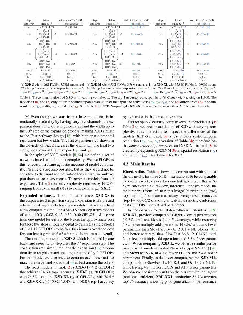
Kinetics-400. Table 4 shows the comparison with state-of-the-art results for three X3D instantiations.To be comparableto previous work, we use the same testing strategy, that is 10-LeftCenterRight (i.e. 30-view) inference. For each model, thetable reports (from-left-to-right) ImageNet pretraining (pre),top-1 and top-5 validation accuracy, average test accuracy as(top-1+ top-5)/2 (i.e. official test-server metric), inferencecost (GFLOPs×views) and parameters.

In comparison to the state-of-the-art, SlowFast [15],X3D-XL, provides comparable (slightly lower) performance(-0.7% top-1 and identical top-5 accuracy), while requiring4.8× fewer multiply-add operations (FLOPs) and 5.5× fewerparameters than SlowFast 16×8, R101 + NL blocks [81],and better accuracy than SlowFast 8×8, R101+NL with2.4× fewer multiply-add operations and 5.5× fewer param-eters. When comparing X3D-L, we observe similar perfor-mance as Channel-Separated Networks (ip-CSN-152) [76]and SlowFast 8×8, at 4.3× fewer FLOPs and 5.4× fewerparameters. Finally, in the lower compute regime X3D-M iscomparable to SlowFast 4×16, R50 and Oct-I3D + NL [9]while having 4.7× fewer FLOPs and 9.1× fewer parameters.We observe consistent results on the test set with the largest(and least efficient) X3D-XXL producing 86.7% averagetop1/5 accuracy, showing good generalization performance.

6

model pre top-1 top-5 test GFLOPs×views ParamI3D [7]

Imag

eNet

71.1 90.3 80.2 108 × N/A 12MTwo-Stream I3D [7] 75.7 92.0 82.8 216 × N/A 25MTwo-Stream S3D-G [89] 77.2 93.0 143 × N/A 23.1MMF-Net [10] 72.8 90.4 11.1 × 50 8.0MTSM R50 [51] 74.7 N/A 65 × 10 24.3MNonlocal R50 [81] 76.5 92.6 282 × 30 35.3MNonlocal R101 [81] 77.7 93.3 83.8 359 × 30 54.3MTwo-Stream I3D [7] - 71.6 90.0 216 × NA 25.0MR(2+1)D [77] - 72.0 90.0 152 × 115 63.6MTwo-Stream R(2+1)D [77] - 73.9 90.9 304 × 115 127.2MOct-I3D + NL [9] - 75.7 N/A 28.9 × 30 33.6Mip-CSN-152 [76] - 77.8 92.8 109 × 30 32.8MSlowFast 4×16, R50 [15] - 75.6 92.1 36.1 × 30 34.4MSlowFast 8×8, R101 [15] - 77.9 93.2 84.2 106 × 30 53.7MSlowFast 8×8, R101+NL [15] - 78.7 93.5 84.9 116 × 30 59.9MSlowFast 16×8, R101+NL [15] - 79.8 93.9 85.7 234 × 30 59.9MX3D-M - 76.0 92.3 82.9 6.2 × 30 3.8MX3D-L - 77.5 92.9 83.8 24.8 × 30 6.1MX3D-XL - 79.1 93.9 85.3 48.4 × 30 11.0MX3D-XXL - 80.4 94.6 86.7 194.1 × 30 20.3MTable 4. Comparison to the state-of-the-art on K400-val & test.We report the inference cost with a single “view" (temporal clip withspatial crop) × the numbers of such views used (GFLOPs×views).“N/A” indicates the numbers are not available for us. The “test”column shows average of top1 and top5 on the Kinetics-400 testset.

model pretrain top-1 top-5 GFLOPs×views ParamI3D [4] - 71.9 90.1 108 × N/A 12MOct-I3D + NL [9] ImageNet 76.0 N/A 25.6 × 30 12MSlowFast 4×16, R50 [15] - 78.8 94.0 36.1 × 30 34.4MSlowFast 16×8, R101+NL [15] - 81.8 95.1 234 × 30 59.9MX3D-M - 78.8 94.5 6.2 × 30 3.8MX3D-XL - 81.9 95.5 48.4 × 30 11.0M

Table 5. Comparison with the state-of-the-art on Kinetics-600.Results are consistent with K400 in Table 4 above.

Kinetics-600 is a larger version of Kinetics that shalldemonstrate further generalization of our approach. Re-sults are shown in Table 5. Our variants demonstrate similarperformance as above, with the best model now providingslightly better performance than the previous state-of-the-art SlowFast 16×8, R101+NL [15], again for 4.8× fewerFLOPs (i.e. multiply-add operations) and 5.5× fewer param-eter. In the lower computation regime, X3D-M is compara-ble to SlowFast 4×16, R50 but requires 5.8× fewer FLOPsand 9.1× fewer parameters.

Charades [62] is a dataset with longer range activities. Ta-ble 6 shows our results. X3D-XL provides higher perfor-mance (+0.9 mAP with K400 and +1.9mAP under K600pretraining), while requiring 4.8× fewer multiply-add op-erations (FLOPs) and 5.5× fewer parameters than previoushighest system, SlowFast [15] with+ NL blocks [81].

4.3. Ablation Experiments

This section provides ablation studies on K400 val andtest sets, comparing accuracy and computational complexity.

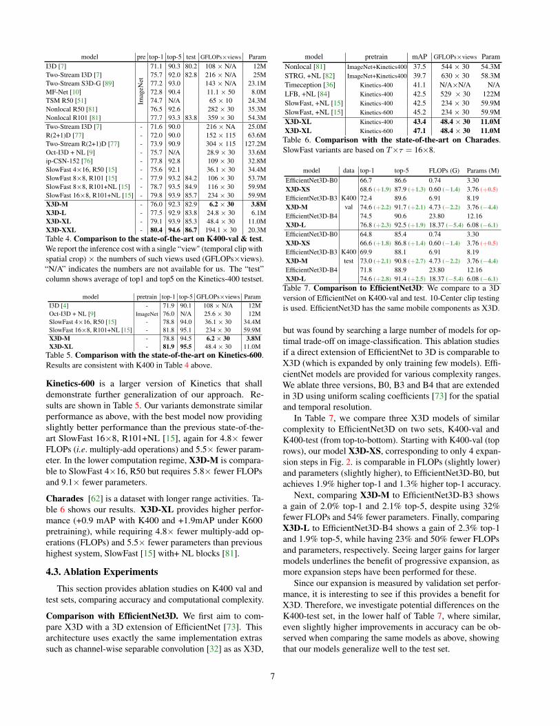
Comparison with EfficientNet3D. We first aim to com-pare X3D with a 3D extension of EfficientNet [73]. Thisarchitecture uses exactly the same implementation extrassuch as channel-wise separable convolution [32] as as X3D,

model pretrain mAP GFLOPs×views ParamNonlocal [81] ImageNet+Kinetics400 37.5 544 × 30 54.3MSTRG, +NL [82] ImageNet+Kinetics400 39.7 630 × 30 58.3MTimeception [36] Kinetics-400 41.1 N/A×N/A N/ALFB, +NL [84] Kinetics-400 42.5 529 × 30 122MSlowFast, +NL [15] Kinetics-400 42.5 234 × 30 59.9MSlowFast, +NL [15] Kinetics-600 45.2 234 × 30 59.9MX3D-XL Kinetics-400 43.4 48.4 × 30 11.0MX3D-XL Kinetics-600 47.1 48.4 × 30 11.0MTable 6. Comparison with the state-of-the-art on Charades.SlowFast variants are based on T×τ = 16×8.

model data top-1 top-5 FLOPs (G) Params (M)EfficientNet3D-B0

K400

66.7 86.6 0.74 3.30X3D-XS

val

68.6 (+1.9) 87.9 (+1.3) 0.60 (−1.4) 3.76 (+0.5)EfficientNet3D-B3 72.4 89.6 6.91 8.19X3D-M 74.6 (+2.2) 91.7 (+2.1) 4.73 (−2.2) 3.76 (−4.4)EfficientNet3D-B4 74.5 90.6 23.80 12.16X3D-L 76.8 (+2.3) 92.5 (+1.9) 18.37 (−5.4) 6.08 (−6.1)EfficientNet3D-B0

K400

64.8 85.4 0.74 3.30X3D-XS

test

66.6 (+1.8) 86.8 (+1.4) 0.60 (−1.4) 3.76 (+0.5)EfficientNet3D-B3 69.9 88.1 6.91 8.19X3D-M 73.0 (+2.1) 90.8 (+2.7) 4.73 (−2.2) 3.76 (−4.4)EfficientNet3D-B4 71.8 88.9 23.80 12.16X3D-L 74.6 (+2.8) 91.4 (+2.5) 18.37 (−5.4) 6.08 (−6.1)

Table 7. Comparison to EfficientNet3D: We compare to a 3Dversion of EfficientNet on K400-val and test. 10-Center clip testingis used. EfficientNet3D has the same mobile components as X3D.

but was found by searching a large number of models for op-timal trade-off on image-classification. This ablation studiesif a direct extension of EfficientNet to 3D is comparable toX3D (which is expanded by only training few models). Effi-cientNet models are provided for various complexity ranges.We ablate three versions, B0, B3 and B4 that are extendedin 3D using uniform scaling coefficients [73] for the spatialand temporal resolution.

In Table 7, we compare three X3D models of similarcomplexity to EfficientNet3D on two sets, K400-val andK400-test (from top-to-bottom). Starting with K400-val (toprows), our model X3D-XS, corresponding to only 4 expan-sion steps in Fig. 2. is comparable in FLOPs (slightly lower)and parameters (slightly higher), to EfficientNet3D-B0, butachieves 1.9% higher top-1 and 1.3% higher top-1 accuracy.

Next, comparing X3D-M to EfficientNet3D-B3 showsa gain of 2.0% top-1 and 2.1% top-5, despite using 32%fewer FLOPs and 54% fewer parameters. Finally, comparingX3D-L to EfficientNet3D-B4 shows a gain of 2.3% top-1and 1.9% top-5, while having 23% and 50% fewer FLOPsand parameters, respectively. Seeing larger gains for largermodels underlines the benefit of progressive expansion, asmore expansion steps have been performed for these.

Since our expansion is measured by validation set perfor-mance, it is interesting to see if this provides a benefit forX3D. Therefore, we investigate potential differences on theK400-test set, in the lower half of Table 7, where similar,even slightly higher improvements in accuracy can be ob-served when comparing the same models as above, showingthat our models generalize well to the test set.

7

76

74

72

70

68

66

Kin

etic

s to

p-1

accu

racy

(%)

78

80

Inference cost per video in TFLOPs (# of multiply-adds x 1012)0.0 0.25 1.00 1.25 1.750.5 0.75 1.50

X3D-XLX3D-MX3D-SSlowFast 16x8, R101+NLSlowFast 8x8, R101+NLSlowFast 8x8, R101CSN (Channel-Separated Networks)TSM (Temporal Shift Module)

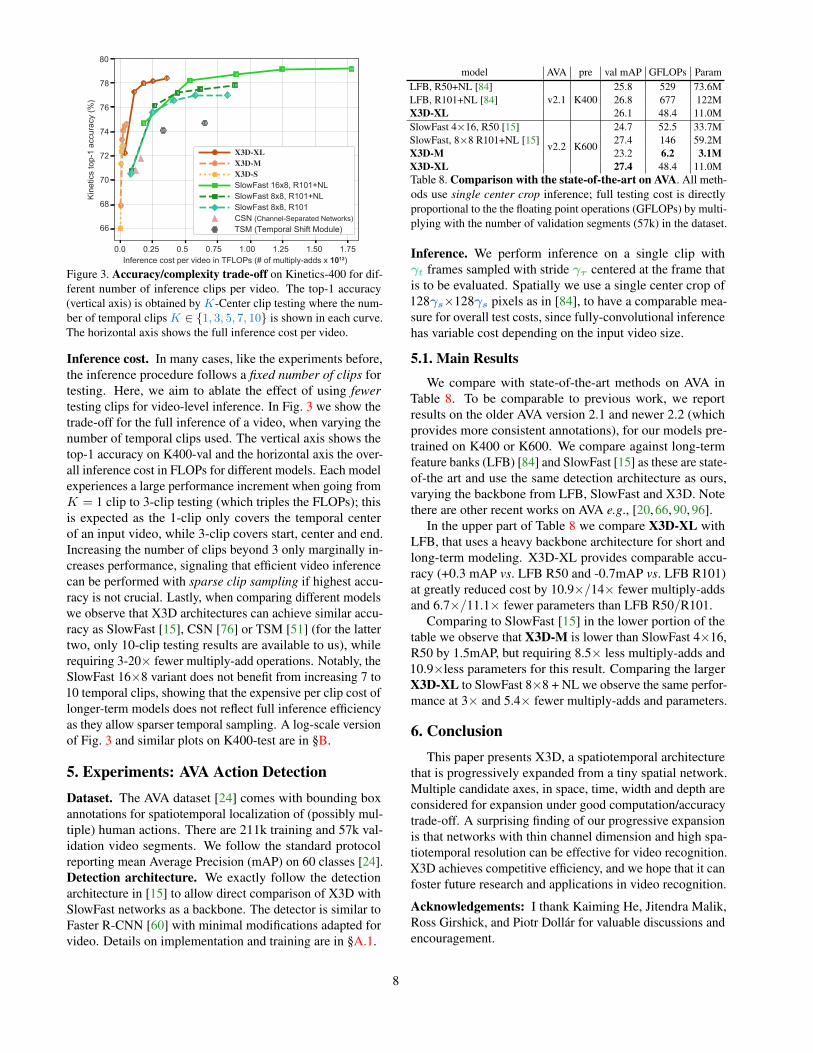
Figure 3. Accuracy/complexity trade-off on Kinetics-400 for dif-ferent number of inference clips per video. The top-1 accuracy(vertical axis) is obtained by K-Center clip testing where the num-ber of temporal clips K ∈ {1, 3, 5, 7, 10} is shown in each curve.The horizontal axis shows the full inference cost per video.

Inference cost. In many cases, like the experiments before,the inference procedure follows a fixed number of clips fortesting. Here, we aim to ablate the effect of using fewertesting clips for video-level inference. In Fig. 3 we show thetrade-off for the full inference of a video, when varying thenumber of temporal clips used. The vertical axis shows thetop-1 accuracy on K400-val and the horizontal axis the over-all inference cost in FLOPs for different models. Each modelexperiences a large performance increment when going fromK = 1 clip to 3-clip testing (which triples the FLOPs); thisis expected as the 1-clip only covers the temporal centerof an input video, while 3-clip covers start, center and end.Increasing the number of clips beyond 3 only marginally in-creases performance, signaling that efficient video inferencecan be performed with sparse clip sampling if highest accu-racy is not crucial. Lastly, when comparing different modelswe observe that X3D architectures can achieve similar accu-racy as SlowFast [15], CSN [76] or TSM [51] (for the lattertwo, only 10-clip testing results are available to us), whilerequiring 3-20× fewer multiply-add operations. Notably, theSlowFast 16×8 variant does not benefit from increasing 7 to10 temporal clips, showing that the expensive per clip cost oflonger-term models does not reflect full inference efficiencyas they allow sparser temporal sampling. A log-scale versionof Fig. 3 and similar plots on K400-test are in §B.

5. Experiments: AVA Action DetectionDataset. The AVA dataset [24] comes with bounding boxannotations for spatiotemporal localization of (possibly mul-tiple) human actions. There are 211k training and 57k val-idation video segments. We follow the standard protocolreporting mean Average Precision (mAP) on 60 classes [24].Detection architecture. We exactly follow the detectionarchitecture in [15] to allow direct comparison of X3D withSlowFast networks as a backbone. The detector is similar toFaster R-CNN [60] with minimal modifications adapted forvideo. Details on implementation and training are in §A.1.

model AVA pre val mAP GFLOPs ParamLFB, R50+NL [84]

v2.1 K40025.8 529 73.6M

LFB, R101+NL [84] 26.8 677 122MX3D-XL 26.1 48.4 11.0MSlowFast 4×16, R50 [15]

v2.2 K600

24.7 52.5 33.7MSlowFast, 8×8 R101+NL [15] 27.4 146 59.2MX3D-M 23.2 6.2 3.1MX3D-XL 27.4 48.4 11.0MTable 8. Comparison with the state-of-the-art on AVA. All meth-ods use single center crop inference; full testing cost is directlyproportional to the the floating point operations (GFLOPs) by multi-plying with the number of validation segments (57k) in the dataset.

Inference. We perform inference on a single clip withγt frames sampled with stride γτ centered at the frame thatis to be evaluated. Spatially we use a single center crop of128γs×128γs pixels as in [84], to have a comparable mea-sure for overall test costs, since fully-convolutional inferencehas variable cost depending on the input video size.

5.1. Main Results

We compare with state-of-the-art methods on AVA inTable 8. To be comparable to previous work, we reportresults on the older AVA version 2.1 and newer 2.2 (whichprovides more consistent annotations), for our models pre-trained on K400 or K600. We compare against long-termfeature banks (LFB) [84] and SlowFast [15] as these are state-of-the art and use the same detection architecture as ours,varying the backbone from LFB, SlowFast and X3D. Notethere are other recent works on AVA e.g., [20, 66, 90, 96].

In the upper part of Table 8 we compare X3D-XL withLFB, that uses a heavy backbone architecture for short andlong-term modeling. X3D-XL provides comparable accu-racy (+0.3 mAP vs. LFB R50 and -0.7mAP vs. LFB R101)at greatly reduced cost by 10.9×/14× fewer multiply-addsand 6.7×/11.1× fewer parameters than LFB R50/R101.

Comparing to SlowFast [15] in the lower portion of thetable we observe that X3D-M is lower than SlowFast 4×16,R50 by 1.5mAP, but requiring 8.5× less multiply-adds and10.9×less parameters for this result. Comparing the largerX3D-XL to SlowFast 8×8 + NL we observe the same perfor-mance at 3× and 5.4× fewer multiply-adds and parameters.

6. ConclusionThis paper presents X3D, a spatiotemporal architecture

that is progressively expanded from a tiny spatial network.Multiple candidate axes, in space, time, width and depth areconsidered for expansion under good computation/accuracytrade-off. A surprising finding of our progressive expansionis that networks with thin channel dimension and high spa-tiotemporal resolution can be effective for video recognition.X3D achieves competitive efficiency, and we hope that it canfoster future research and applications in video recognition.

Acknowledgements: I thank Kaiming He, Jitendra Malik,Ross Girshick, and Piotr Dollár for valuable discussions andencouragement.

8

Appendix

This appendix provides further details as referenced inthe main paper: Sec. A contains additional implementationdetails for: AVA Action Detection (§A.1), Charades ActionClassification (§A.2), and Kinetics Action Classification(§A.3). Sec. B contains further results and ablations onKinetics-400.

A. Additional Implementation Details

A.1. Details: AVA Action Detection

Detection architecture. We exactly follow the detectionarchitecture in [15] to allow direct comparison of X3D withSlowFast networks as a backbone. The detector is similarto Faster R-CNN [60] with minimal modifications adaptedfor video. Since our paper focuses on efficiency, by default,we do not increase the spatial resolution of res5 by 2× [15].Region-of-interest (RoI) features [21] are extracted at thelast feature map of res5 by extending a 2D proposal at aframe into a 3D RoI by replicating it along the temporal axis,similar as done in previous work [24, 40, 66], followed byapplication of frame-wise RoIAlign [27] and temporal globalaverage pooling. The RoI features are then max-pooled andfed to a per-class, sigmoid classifier for prediction.

Training. For direct comparison, the training procedure andhyper-parameters for AVA follow [15] without modification.The network weights are initialized from the Kinetics modelsand we use step-wise learning rate decay, that is reducedby 10× when validation error saturates. We train for 14kiterations (68 epochs for ∼211k data), with linear warm-up[23] for the first 1k iterations and use a weight decay of 10−7,as in [15]. All other hyper-parameters are the same as in theKinetics experiments. Ground-truth boxes, and proposalsoverlapping with ground-truth boxes by IoU > 0.9, are usedas the samples for training. The inputs are instantiation-specific clips of size γt×112γs×112γswith time stride γτ .

The region proposal extraction also follows [15] and issummarized here for completeness. We follow previousworks that use pre-computed proposals [24, 40, 66]. Ourregion proposals are computed by an off-the-shelf person de-tector, i.e., that is not jointly trained with the action detectionmodels. We adopt a person-detection model trained withDetectron [22]. It is a Faster R-CNN with a ResNeXt-101-FPN [52, 88] backbone. It is pre-trained on ImageNet andthe COCO human keypoint images [53]. We fine-tune thisdetector on AVA for person (actor) detection. The persondetector produces 93.9 AP@50 on the AVA validation set.Then, the region proposals for action detection are detectedperson boxes with a confidence of > 0.8, which has a recallof 91.1% and a precision of 90.7% for the person class.

A.2. Details: Charades Action Classification

For Charades, we fine-tune the Kinetics models. Allsettings are the same as those of Kinetics, except the fol-lowing. A per-class sigmoid output is used to account forthe mutli-class nature. We train on a single machine for24k iterations using a batch size of 16 and a base learningrate of 0.02 with 10× step-wise decay if the validation errorsaturates. We use weight decay of 10-5. We also increasethe model temporal stride by ×2 as this dataset benefitsfrom longer clips. For inference, we temporally max-poolprediction scores [15, 81].

A.3. Details: Kinetics Action Classification

Training details. We use the initialization in [28]. Weadopt synchronized SGD training on 128 GPUs followingthe recipe in [23]. The mini-batch size is 8 clips per GPU(so the total mini-batch size is 1024). We train with BatchNormalization (BN) [38], and the BN statistics are computedwithin each 8 clips, unless noted otherwise. We adopt a half-period cosine schedule [54] of learning rate decaying: thelearning rate at the n-th iteration is η · 0.5[cos( n

nmaxπ) + 1],

where nmax is the maximum training iterations and the baselearning rate η is set as 1.6. We also use a linear warm-upstrategy [23] in the first 8k iterations. Unless specified, wetrain for 256 epochs (60k iterations with a total mini-batchsize of 1024, in ∼240k Kinetics videos). We use momentumof 0.9, weight decay of 5×10-5 and dropout [30] of 0.5 isused before the final classifier.

For Kinetics-600, we extend the training epochs (andschedule) of above by 2×. All other hyper-parameters areexactly as for Kinetics-400.

Implementation details. Non-Local (NL) blocks [81] arenot used for X3D. For SlowFast results, we use exactly thesame implementation details as in [15]. Specifically, forSlowFast models involving NL, we initialize them with thecounterparts that are trained without NL, to facilitate conver-gence. We only use NL on the (fused) Slow features of res4(instead of res3+res4 [81]). For X3D and EfficientNet3D, wefollow previous work on 2D mobile architectures [31,72,73],using SE blocks [33] (also found beneficial for efficientvideo classification in [89]) and swish non-linearity [59]. Toconserve memory, we use SE with original reduction ratio of1/16 only in every other residual block after the 3×32 conv;swish is only used before and after these layers and all otherweight layers are followed by ReLU non-linearity [47]. Wedo not employ the “linear-bottleneck” design used in mobileimage networks [31, 61, 72, 73], as we found it to sometimescause instability in distributed training, as it does not allowto zero-initialize the final BN scaling [23] of residual blocks.

Expansion details. To expand the model specified in Ta-ble 1, we set all initial expansion factors, X0, to one i.e.γt=γs=γw=γb=γd=1 resulting in the X2D base model.

9

A temporal sampling rate γτ is not defined for the X2Dmodel as it does not have multiple frames. The smallestpossible common expansion for this model is defined byincreasing the number of frames from 1 to two; therefore weset the expansion-rate c to match the cost of increasing thetemporal input length of the model by a factor of two (thesmallest possible common increase in the first expansionstep), which roughly doubles the cost of the model, c = 2.

Then, in every step of our expansion we train a models,one for expanding each axis, such that its complexity doubles(c = 2). For the individual axes this roughly3 equals to thefollowing operations:

• X-Fast: γτ← 0.5γτ , reduces the sampling stride todouble frame-rate while sampling the same input dura-tion, this doubles the temporal size γt←2γt.

• X-Temporal: Increases frame-rate by γτ← 0.75γτ andinput duration to double the input size γt←2γt (i.e.1.5× higher frame-rate and 1.5×longer input duration).

• X-Spatial: Expands the spatial resolution proportionallyγs←

√2γs.

• X-Depth: Expands the depth of the network by aroundγd← 2.2γd.

• X-Width: Expands the global width for all layers byγw← 2γw.

• X-Bottleneck: Expands the bottleneck width by roughlyγb← 2.25γb.

The exact scaling factors slightly differ from one expan-sion step to the other due to rounding effects in networkgeometry (layers stride, activation size etc.).

Since the stepwise expansion also allows to elegantly in-tegrate regularization (which is typically increased for largermodels), we perform a regularization expansion if the train-ing error of the previous expansion step starts to deviate fromthe validation error. Specifically, we start the expansion withdouble the batch-size and half learning schedule than de-scribed above, then the BN statistics are computed withineach 16 clips which lowers regularization and improves per-formance on small models. The batch-size is then decreasedby 2× at the 8th step of expansion which increases general-ization. We perform another regularization expansion at the11th/13th step by using drop-connect with rate 0.1/0.2 [34].

B. Additional ResultsFig. A.4 shows a series of extra plots on Kinetics-400,

analyzed next (this extends Sec. 4 of the main paper):

3The exact expansion factors slightly vary across steps to match thecomplexity increase, c (which is observable in Fig. 2 of the main paper).

Inference cost. Here we aim to provide further ablationsfor the effect of using fewer testing clips for efficient video-level inference. In Fig. A.4 we show the trade-off for the fullinference of a video, when varying the number of temporalclips used. The vertical axis shows the top-1 accuracy onK400-val and the horizontal axis the overall inference costin FLOPs for different models.

First, for comparison, the plot on top-left is the same asthe one shown in Fig. 3. The plot on top-right shows thissame plot with a logarithmic scale applied to the FLOPs axis.Using this scaling it is clearer to observe that smaller models(X3D-S and X3D-M) can provide up to 20× reduction interms of multiply-add operations used during inference.

For example, 3-clip X3D-S produces 71.4% top-1 at 5.9GFLOPs, whereas 10-clip CSN-50 [76] produces 70.8 top-1at 119 GFLOPs (20.2× higher cost), or 10-clip X3D-S 72.9%top-1 at 19.6 GFLOPs, and 10-clip CSN-101 [76] 71.8%top-1 at 159 GFLOPs (8.1× higher cost).

The lower two plots in Fig. A.4 show the identical resultson the test set of Kinetics-400 (which has been publiclyreleased with Kinetics-600 [4]). Note that the test set is morechallenging which leads to overall lower accuracy for allapproaches [1]. We observe consistent results on the test set,illustrating good generalization of the models.

Mobile components. Finally, we ablate the effect ofmobile components employed in X3D and EfficientNet3D.Since the components can have different effects of modelsfrom the small and large computation regime, we ablate theeffects on a small (X3D-S) and a large model (X3D-XL).

First, we ablate channel-wise separable convolution [32],a key component in mobile ConvNets. We ablate two ver-sions: (i) A version that reduces the bottleneck ratio (γb)accordingly, such that the overall architecture preserves themultiple-add operations (FLOPs), and (ii) a version thatkeeps the originally, expanded bottleneck ratio.

Table A.1 shows the results. For case (i) we see thatperformance drops significantly by 4% top-1 accuracy forX3D-S and by 2.4% for X3D-XL. For case (ii), we see thatthe performance of the baselines increases by 0.3% and0.8% top-1 accuracy for X3D-S and X3D-XL, respectively.This shows that separable convolution is important for small-computation budgets, however, for best-performance a non-separable convolution can provide gains (at high cost).

Second, we ablate swish non-linearities [59] (that are onlyimplemented before and after the “bottleneck” convolution,to conserve memory). We observe that removing swish hasa smaller performance decrease of 0.9% for X3D-S and0.4% for X3D-XL, and therefore could be changed to ReLU(which can be implemented in-place) if memory is priority.

Third, we ablate SE blocks [33] (that are only used in ev-ery other residual block, to conserve memory). We observethat removing SE has a larger effect on performance, decreas-ing accuracy by 1.6% for X3D-S and 1.3% for X3D-XL.

10

Inference cost per video in TFLOPs (# of multiply-adds x 1012)0.0 0.2 0.4 0.6 0.8

76

74

72

70

68

66

64

Kin

etic

s to

p-1

val a

ccur

acy

(%) 78

80

SlowFast 8x8, R101+NLSlowFast 8x8, R101

X3D-XLX3D-M

EfficientNet3D-B4EfficientNet3D-B3

X3D-S

CSN (Channel-Separated Networks)TSM (Temporal Shift Module)

Inference cost per video in FLOPs (# of multiply-adds), log-scale

SlowFast 8x8, R101+NLSlowFast 8x8, R101

X3D-XLX3D-M

EfficientNet3D-B4EfficientNet3D-B3

X3D-S

CSN (Channel-Separated Networks)TSM (Temporal Shift Module)

75

70

65

60

55

50

45

Kin

etic

s to

p-1

val a

ccur

acy

(%)

80

401010 1011 1012

76

74

72

70

68

66

64

Kin

etic

s to

p-1

test

acc

urac

y (%

)

78

Inference cost per video in TFLOPs (# of multiply-adds x 1012)0.0 0.2 0.4 0.6 0.8

SlowFast 8x8, R101+NLSlowFast 8x8, R101

X3D-XLX3D-M

EfficientNet3D-B4EfficientNet3D-B3

X3D-SSlowFast 8x8, R101+NLSlowFast 8x8, R101

X3D-XLX3D-M

EfficientNet3D-B4EfficientNet3D-B3

X3D-S

75

70

65

60

55

50

45

Kin

etic

s to

p-1

test

acc

urac

y (%

)

80

40

Inference cost per video in FLOPs (# of multiply-adds), log-scale1010 1011 1012

Figure A.4. Accuracy/complexity trade-off on K400-val (top) & test (bottom) for varying # of inference clips per video. The top-1accuracy (vertical axis) is obtained by K-Center clip testing where the number of temporal clips K ∈ {1, 3, 5, 7, 10} is shown in each curve.The horizontal axis measures the full inference cost per video. The left-sided plots show a linear and the right plots a logarithmic (log) scale.

These observed effects on performance are similar to theones that have been shown Non-local (NL) attention blocks[81], and also in line with [89], where SE attention blockshave been found beneficial for efficient video classification.

References

[1] ActivityNet-Challenge. http://activity-net.org/challenges/2017/evaluation.html, 2017. 10

[2] Humam Alwassel, Fabian Caba Heilbron, and BernardGhanem. Action search: Spotting actions in videos and itsapplication to temporal action localization. In Proc. ECCV,2018. 2

[3] H. Bilen, B. Fernando, E. Gavves, A. Vedaldi, and S. Gould.Dynamic image networks for action recognition. In Proc.CVPR, 2016. 2

[4] Joao Carreira, Eric Noland, Andras Banki-Horvath, ChloeHillier, and Andrew Zisserman. A short note about Kinetics-600. arXiv:1808.01340, 2018. 2, 5, 7, 10

[5] Joao Carreira, Eric Noland, Chloe Hillier, and Andrew Zisser-man. A short note on the kinetics-700 human action dataset.arXiv preprint arXiv:1907.06987, 2019. 2

[6] Joao Carreira, Viorica Patraucean, Laurent Mazare, AndrewZisserman, and Simon Osindero. Massively parallel videonetworks. In Proc. ECCV, 2018. 2

[7] Joao Carreira and Andrew Zisserman. Quo vadis, actionrecognition? a new model and the kinetics dataset. In Proc.CVPR, 2017. 1, 2, 4, 7

[8] K. Chatfield, K. Simonyan, A. Vedaldi, and A. Zisserman.Return of the devil in the details: Delving deep into convolu-tional nets. In Proc. BMVC., 2014. 2, 3, 6

[9] Yunpeng Chen, Haoqi Fang, Bing Xu, Zhicheng Yan, Yan-nis Kalantidis, Marcus Rohrbach, Shuicheng Yan, and Jiashi

11

model top-1 top-5 FLOPs (G) Param (M)X3D-S 72.9 90.5 1.96 3.76− CW conv γb= 0.6 68.9 88.8 1.95 3.16

− CW conv 73.2 90.4 17.6 22.1− swish 72.0 90.4 1.96 3.76− SE 71.3 89.9 1.96 3.60

(a) Ablating mobile components on a Small model.

model top-1 top-5 FLOPs (G) Param (M)X3D-XL 78.4 93.6 35.84 11.0− CW conv, γb= 0.56 76.0 92.6 34.80 9.73

− CW conv 79.2 93.5 365.4 95.1− swish 78.0 93.4 35.84 11.0− SE 77.1 93.0 35.84 10.4

(b) Ablating mobile components on an X-Large model.

Table A.1. Ablations of mobile components for video classification on K400-val. We show top-1 and top-5 classification accuracy (%),parameters, and computational complexity measured in GFLOPs (floating-point operations, in # of multiply-adds ×109) for a single clipinput of size γt×112γs×112γx. Inference-time computational cost is reported GFLOPs×10, as a fixed number of 10-Center views is used.The results show that removing channel-wise separable convolution (CW conv) with unchanged bottleneck expansion ratio, γb, drasticallyincreases mutliply-adds and parameters at slightly higher accuracy, while swish has a smaller effect on performance than SE.

Feng. Drop an octave: Reducing spatial redundancy in con-volutional neural networks with octave convolution. arXivpreprint arXiv:1904.05049, 2019. 6, 7

[10] Yunpeng Chen, Yannis Kalantidis, Jianshu Li, Shuicheng Yan,and Jiashi Feng. Multi-fiber networks for video recognition.In Proc. ECCV, 2018. 2, 7

[11] J. Deng, W. Dong, R. Socher, L.-J. Li, K. Li, and L. Fei-Fei.ImageNet: A large-scale hierarchical image database. In Proc.CVPR, 2009. 5

[12] Ali Diba, Mohsen Fayyaz, Vivek Sharma, M Mahdi Arzani,Rahman Yousefzadeh, Juergen Gall, and Luc Van Gool.Spatio-temporal channel correlation networks for action clas-sification. In Proc. ECCV, 2018. 2

[13] Jeff Donahue, Lisa Anne Hendricks, Sergio Guadarrama, Mar-cus Rohrbach, Subhashini Venugopalan, Kate Saenko, andTrevor Darrell. Long-term recurrent convolutional networksfor visual recognition and description. In Proc. CVPR, 2015.1, 2

[14] Lijie Fan, Wenbing Huang, Chuang Gan, Stefano Ermon,Boqing Gong, and Junzhou Huang. End-to-end learningof motion representation for video understanding. In Proc.CVPR, 2018. 2

[15] Christoph Feichtenhofer, Haoqi Fan, Jitendra Malik, andKaiming He. SlowFast networks for video recognition. InProc. ICCV, 2019. 2, 3, 4, 5, 6, 7, 8, 9

[16] Christoph Feichtenhofer, Haoqi Fan, Jitendra Ma-lik, and Kaiming He. SlowFast networks forvideo recognition in ActivityNet challenge 2019.http://static.googleusercontent.com/media/research.google.com/en//ava/2019/fair_slowfast.pdf, 2019. 6

[17] Christoph Feichtenhofer, Axel Pinz, and Richard Wildes. Spa-tiotemporal residual networks for video action recognition.In NIPS, 2016. 1, 2, 4

[18] Christoph Feichtenhofer, Axel Pinz, and Andrew Zisserman.Convolutional two-stream network fusion for video actionrecognition. In Proc. CVPR, 2016. 2

[19] Basura Fernando, Efstratios Gavves, Jose M Oramas, AmirGhodrati, and Tinne Tuytelaars. Modeling video evolution foraction recognition. In IEEE PAMI, pages 5378–5387, 2015. 2

[20] Rohit Girdhar, João Carreira, Carl Doersch, and AndrewZisserman. Video action transformer network. In Proc. CVPR,2019. 8

[21] Ross Girshick. Fast R-CNN. In Proc. ICCV, 2015. 9[22] Ross Girshick, Ilija Radosavovic, Georgia Gkioxari, Piotr

Dollár, and Kaiming He. Detectron. https://github.com/facebookresearch/detectron, 2018. 9

[23] Priya Goyal, Piotr Dollár, Ross Girshick, Pieter Noord-huis, Lukasz Wesolowski, Aapo Kyrola, Andrew Tulloch,Yangqing Jia, and Kaiming He. Accurate, large minibatchSGD: training ImageNet in 1 hour. arXiv:1706.02677, 2017.9

[24] Chunhui Gu, Chen Sun, David A. Ross, Carl Vondrick, Car-oline Pantofaru, Yeqing Li, Sudheendra Vijayanarasimhan,George Toderici, Susanna Ricco, Rahul Sukthankar, CordeliaSchmid, and Jitendra Malik. AVA: A video dataset of spatio-temporally localized atomic visual actions. In Proc. CVPR,2018. 2, 8, 9

[25] Isabelle Guyon and André Elisseeff. An introduction to vari-able and feature selection. Journal of machine learning re-search, 3(Mar):1157–1182, 2003. 2, 4

[26] Kensho Hara, Hirokatsu Kataoka, and Yutaka Satoh. Canspatiotemporal 3d cnns retrace the history of 2d cnns andimagenet? In Proc. CVPR, 2018. 2

[27] Kaiming He, Georgia Gkioxari, Piotr Dollár, and Ross Gir-shick. Mask R-CNN. In Proc. ICCV, 2017. 9

[28] Kaiming He, Xiangyu Zhang, Shaoqing Ren, and Jian Sun.Delving deep into rectifiers: Surpassing human-level perfor-mance on imagenet classification. In Proc. CVPR, 2015. 9

[29] Kaiming He, Xiangyu Zhang, Shaoqing Ren, and Jian Sun.Deep residual learning for image recognition. In Proc. CVPR,2016. 1, 2, 3, 5

[30] Geoffrey E Hinton, Nitish Srivastava, Alex Krizhevsky, IlyaSutskever, and Ruslan R Salakhutdinov. Improving neuralnetworks by preventing co-adaptation of feature detectors.arXiv:1207.0580, 2012. 9

[31] Andrew Howard, Mark Sandler, Grace Chu, Liang-ChiehChen, Bo Chen, Mingxing Tan, Weijun Wang, Yukun Zhu,Ruoming Pang, Vijay Vasudevan, Quoc V. Le, and HartwigAdam. Searching for MobileNetV3. arXiv:1905.02244, 2019.1, 2, 3, 4, 9

[32] Andrew G Howard, Menglong Zhu, Bo Chen, DmitryKalenichenko, Weijun Wang, Tobias Weyand, Marco An-dreetto, and Hartwig Adam. MobileNets: Efficient convolu-tional neural networks for mobile vision applications. arXivpreprint arXiv:1704.04861, 2017. 1, 2, 3, 4, 7, 10

12

[33] Jie Hu, Li Shen, and Gang Sun. Squeeze-and-excitationnetworks. In Proc. CVPR, 2018. 2, 9, 10

[34] Gao Huang, Yu Sun, Zhuang Liu, Daniel Sedra, and Kilian QWeinberger. Deep networks with stochastic depth. In Proc.ECCV, 2016. 10

[35] Yanping Huang, Yonglong Cheng, Dehao Chen, HyoukJoongLee, Jiquan Ngiam, Quoc V Le, and Zhifeng Chen. Gpipe:Efficient training of giant neural networks using pipelineparallelism. arXiv preprint arXiv:1811.06965, 2018. 2, 3

[36] Noureldien Hussein, Efstratios Gavves, and Arnold WMSmeulders. Timeception for complex action recognition. InProc. CVPR, 2019. 2, 7

[37] Forrest N. Iandola, Song Han, Matthew W. Moskewicz,Khalid Ashraf, William J. Dally, and Kurt Keutzer.Squeezenet: Alexnet-level accuracy with 50x fewer parame-ters and <0.5mb model size. arXiv:1602.07360, 2016. 3

[38] Sergey Ioffe and Christian Szegedy. Batch normalization:Accelerating deep network training by reducing internal co-variate shift. In Proc. ICML, 2015. 9

[39] Anil Jain and Douglas Zongker. Feature selection: Eval-uation, application, and small sample performance. IEEEtransactions on pattern analysis and machine intelligence,19(2):153–158, 1997. 4

[40] Huaizu Jiang, Deqing Sun, Varun Jampani, Ming-Hsuan Yang,Erik Learned-Miller, and Jan Kautz. Super slomo: Highquality estimation of multiple intermediate frames for videointerpolation. In Proc. CVPR, 2018. 9

[41] George H John, Ron Kohavi, and Karl Pfleger. Irrelevant fea-tures and the subset selection problem. In Machine LearningProceedings 1994, pages 121–129. Elsevier, 1994. 2, 4

[42] Andrej Karpathy, George Toderici, Sanketh Shetty, ThomasLeung, Rahul Sukthankar, and Li Fei-Fei. Large-scale videoclassification with convolutional neural networks. In Proceed-ings of the IEEE conference on Computer Vision and PatternRecognition, pages 1725–1732, 2014. 1, 3

[43] Will Kay, Joao Carreira, Karen Simonyan, Brian Zhang,Chloe Hillier, Sudheendra Vijayanarasimhan, Fabio Viola,Tim Green, Trevor Back, Paul Natsev, et al. The kineticshuman action video dataset. arXiv:1705.06950, 2017. 2, 4

[44] Ron Kohavi and George H John. Wrappers for feature subsetselection. Artificial intelligence, 97(1-2):273–324, 1997. 2, 4

[45] Okan Köpüklü, Neslihan Kose, Ahmet Gunduz, and GerhardRigoll. Resource efficient 3d convolutional neural networks.arXiv preprint arXiv:1904.02422, 2019. 2, 4

[46] Bruno Korbar, Du Tran, and Lorenzo Torresani. Scsampler:Sampling salient clips from video for efficient action recogni-tion. In Proc. ICCV, 2019. 2, 5

[47] Alex Krizhevsky, Ilya Sutskever, and Geoffrey E Hinton. Ima-geNet classification with deep convolutional neural networks.In NIPS, 2012. 1, 2, 3, 9

[48] Myunggi Lee, Seungeui Lee, Sungjoon Son, Gyutae Park,and Nojun Kwak. Motion feature network: Fixed motionfilter for action recognition. In Proc. ECCV, 2018. 2

[49] Dong Li, Zhaofan Qiu, Qi Dai, Ting Yao, and Tao Mei. Re-current tubelet proposal and recognition networks for actiondetection. In Proc. ECCV, 2018. 2

[50] Zhenyang Li, Kirill Gavrilyuk, Efstratios Gavves, Mihir Jain,and Cees GM Snoek. VideoLSTM convolves, attends andflows for action recognition. Computer Vision and ImageUnderstanding, 166:41–50, 2018. 2

[51] Ji Lin, Chuang Gan, and Song Han. Temporal shift modulefor efficient video understanding. In Proc. ICCV, 2019. 2, 5,7, 8

[52] Tsung-Yi Lin, Piotr Dollár, Ross Girshick, Kaiming He,Bharath Hariharan, and Serge Belongie. Feature pyramidnetworks for object detection. In Proc. CVPR, 2017. 9

[53] Tsung-Yi Lin, Michael Maire, Serge Belongie, James Hays,Pietro Perona, Deva Ramanan, Piotr Dollár, and C LawrenceZitnick. Microsoft COCO: Common objects in context. InProc. ECCV, 2014. 9

[54] Ilya Loshchilov and Frank Hutter. SGDR: Stochastic gradientdescent with warm restarts. arXiv:1608.03983, 2016. 9

[55] Chenxu Luo and Alan L. Yuille. Grouped spatial-temporalaggregation for efficient action recognition. In Proc. ICCV,2019. 2

[56] Joe Yue-Hei Ng, Matthew Hausknecht, Sudheendra Vijaya-narasimhan, Oriol Vinyals, Rajat Monga, and George Toderici.Beyond short snippets: Deep networks for video classification.In Proc. CVPR, 2015. 1, 2

[57] AJ Piergiovanni and Michael S. Ryoo. Representation flowfor action recognition. In The IEEE Conference on ComputerVision and Pattern Recognition (CVPR), June 2019. 2

[58] Zhaofan Qiu, Ting Yao, and Tao Mei. Learning spatio-temporal representation with pseudo-3d residual networks. InProc. ICCV, 2017. 2

[59] Prajit Ramachandran, Barret Zoph, and Quoc V Le. Searchingfor activation functions. arXiv preprint arXiv:1710.05941,2017. 2, 9, 10

[60] Shaoqing Ren, Kaiming He, Ross Girshick, and Jian Sun.Faster R-CNN: Towards real-time object detection with regionproposal networks. In NIPS, 2015. 8, 9

[61] Mark Sandler, Andrew Howard, Menglong Zhu, Andrey Zh-moginov, and Liang-Chieh Chen. MobileNetV2: Invertedresiduals and linear bottlenecks. In Proc. CVPR, 2018. 1, 2,3, 4, 5, 9

[62] Gunnar A Sigurdsson, Gül Varol, Xiaolong Wang, AliFarhadi, Ivan Laptev, and Abhinav Gupta. Hollywood inhomes: Crowdsourcing data collection for activity under-standing. In ECCV, 2016. 2, 7

[63] Karen Simonyan and Andrew Zisserman. Two-stream convo-lutional networks for action recognition in videos. In NIPS,2014. 2, 3

[64] Karen Simonyan and Andrew Zisserman. Very deep convo-lutional networks for large-scale image recognition. In Proc.ICLR, 2015. 1, 2, 3, 5, 6

[65] Yu-Chuan Su and Kristen Grauman. Leaving some stonesunturned: dynamic feature prioritization for activity detectionin streaming video. In Proc. ECCV, 2016. 2

[66] Chen Sun, Abhinav Shrivastava, Carl Vondrick, Kevin Mur-phy, Rahul Sukthankar, and Cordelia Schmid. Actor-centricrelation network. In ECCV, 2018. 8, 9

[67] Lin Sun, Kui Jia, Kevin Chen, Dit-Yan Yeung, Bertram EShi, and Silvio Savarese. Lattice long short-term memory forhuman action recognition. In Proc. ICCV, 2017. 2

13

[68] Lin Sun, Kui Jia, Dit-Yan Yeung, and Bertram Shi. Humanaction recognition using factorized spatio-temporal convolu-tional networks. In Proc. ICCV, 2015. 2

[69] Shuyang Sun, Zhanghui Kuang, Lu Sheng, Wanli Ouyang,and Wei Zhang. Optical flow guided feature: A fast and robustmotion representation for video action recognition. In Proc.CVPR, 2018. 2

[70] Christian Szegedy, Sergey Ioffe, and Vincent Vanhoucke.Inception-v4, inception-resnet and the impact of residual con-nections on learning. arXiv:1602.07261, 2016. 2, 3

[71] Christian Szegedy, Wei Liu, Yangqing Jia, Pierre Sermanet,Scott Reed, Dragomir Anguelov, Dumitru Erhan, VincentVanhoucke, and Andrew Rabinovich. Going deeper withconvolutions. In Proc. CVPR, 2015. 1, 2, 3

[72] Mingxing Tan, Bo Chen, Ruoming Pang, Vijay Vasudevan,Mark Sandler, Andrew Howard, and Quoc V Le. MnasNet:Platform-aware neural architecture search for mobile. In Proc.CVPR, 2019. 2, 9

[73] Mingxing Tan and Quoc V Le. Efficientnet: Rethinking modelscaling for convolutional neural networks. arXiv preprintarXiv:1905.11946, 2019. 2, 3, 7, 9

[74] Graham W Taylor, Rob Fergus, Yann LeCun, and ChristophBregler. Convolutional learning of spatio-temporal features.In Proc. ECCV, 2010. 2

[75] Du Tran, Lubomir Bourdev, Rob Fergus, Lorenzo Torresani,and Manohar Paluri. Learning spatiotemporal features with3D convolutional networks. In Proc. ICCV, 2015. 1, 2, 3, 4

[76] Du Tran, Heng Wang, Lorenzo Torresani, and Matt Feiszli.Video classification with channel-separated convolutional net-works. In Proc. ICCV, 2019. 2, 4, 5, 6, 7, 8, 10

[77] Du Tran, Heng Wang, Lorenzo Torresani, Jamie Ray, YannLeCun, and Manohar Paluri. A closer look at spatiotemporalconvolutions for action recognition. In Proc. CVPR, 2018. 3,7

[78] Heng Wang, Du Tran, Lorenzo Torresani, and Matt Feiszli.Video modeling with correlation networks. arXiv preprintarXiv:1906.03349, 2019. 2

[79] Limin Wang, Wei Li, Wen Li, and Luc Van Gool. Appearance-and-relation networks for video classification. In Proc. CVPR,2018. 2

[80] Limin Wang, Yuanjun Xiong, Zhe Wang, Yu Qiao, Dahua Lin,Xiaoou Tang, and Luc Val Gool. Temporal segment networks:Towards good practices for deep action recognition. In Proc.ECCV, 2016. 2

[81] Xiaolong Wang, Ross Girshick, Abhinav Gupta, and KaimingHe. Non-local neural networks. In Proc. CVPR, 2018. 1, 2,4, 5, 6, 7, 9, 11

[82] Xiaolong Wang and Abhinav Gupta. Videos as space-timeregion graphs. In Proc. ECCV, 2018. 7

[83] Stephen J Wright. Coordinate descent algorithms. Mathemat-ical Programming, 151(1):3–34, 2015. 1, 4

[84] Chao-Yuan Wu, Christoph Feichtenhofer, Haoqi Fan, Kaim-ing He, Philipp Krähenbühl, and Ross Girshick. Long-termfeature banks for detailed video understanding. In Proc.CVPR, 2019. 2, 5, 7, 8

[85] Chao-Yuan Wu, Manzil Zaheer, Hexiang Hu, R Manmatha,Alexander J Smola, and Philipp Krähenbühl. Compressedvideo action recognition. In CVPR, 2018. 2

[86] Wenhao Wu, Dongliang He, Xiao Tan, Shifeng Chen, andShilei Wen. Multi-agent reinforcement learning based framesampling for effective untrimmed video recognition. In Proc.ICCV, 2019. 2

[87] Zuxuan Wu, Caiming Xiong, Chih-Yao Ma, Richard Socher,and Larry S Davis. Adaframe: Adaptive frame selection forfast video recognition. In Proc. CVPR, 2019. 2

[88] Saining Xie, Ross Girshick, Piotr Dollár, Zhuowen Tu, andKaiming He. Aggregated residual transformations for deepneural networks. In Proc. CVPR, 2017. 2, 3, 9

[89] Saining Xie, Chen Sun, Jonathan Huang, Zhuowen Tu, andKevin Murphy. Rethinking spatiotemporal feature learningfor video understanding. arXiv:1712.04851, 2017. 2, 7, 9, 11

[90] Xitong Yang, Xiaodong Yang, Ming-Yu Liu, Fanyi Xiao,Larry S Davis, and Jan Kautz. Step: Spatio-temporal progres-sive learning for video action detection. In Proc. CVPR, 2019.8

[91] Serena Yeung, Olga Russakovsky, Greg Mori, and Li Fei-Fei.End-to-end learning of action detection from frame glimpsesin videos. In Proc. CVPR, 2016. 2

[92] Jason Yosinski, Jeff Clune, Anh Nguyen, Thomas Fuchs, andHod Lipson. Understanding neural networks through deepvisualization. In ICML Workshop, 2015. 2

[93] Sergey Zagoruyko and Nikos Komodakis. Wide residualnetworks. In Proc. BMVC., 2016. 2, 3

[94] Matthew D Zeiler. Adadelta: an adaptive learning rate method.arXiv:1212.5701, 2012. 2, 3

[95] Xiangyu Zhang, Xinyu Zhou, Mengxiao Lin, and Jian Sun.Shufflenet: An extremely efficient convolutional neural net-work for mobile devices. In Proc. CVPR, 2018. 2, 3, 4

[96] Yubo Zhang, Pavel Tokmakov, Martial Hebert, and CordeliaSchmid. A structured model for action detection. In Proc.CVPR, 2019. 8

[97] Linchao Zhu, Laura Sevilla-Lara, Du Tran, Matt Feiszli, YiYang, and Heng Wang. Faster recurrent networks for videoclassification. arXiv preprint arXiv:1906.04226, 2019. 2

[98] Yi Zhu, Zhenzhong Lan, Shawn Newsam, and Alexander GHauptmann. Hidden two-stream convolutional networks foraction recognition. arXiv preprint arXiv:1704.00389, 2017. 2

[99] Mohammadreza Zolfaghari, Kamaljeet Singh, and ThomasBrox. ECO: efficient convolutional network for online videounderstanding. In Proc. ECCV, 2018. 2

14