chord transition features for style classi cation of music ... · chord progressions carry...
TRANSCRIPT

Friedrich-Alexander-Universitat Erlangen-Nurnberg
Master Thesis
Chord Transition Features forStyle Classification of Music Recordings
submitted by
Fabian Brand
submitted
October 12, 2018
Supervisor / Advisor
Dr.-Ing. Christof Weiß
Reviewers
Prof. Dr. Meinard Muller
International Audio Laboratories ErlangenA joint institution of the
Friedrich-Alexander-Universitat Erlangen-Nurnberg (FAU) andthe Fraunhofer-Institut fur Integrierte Schaltungen IIS.


ERKLARUNG
Erklarung
Ich versichere, dass ich die Arbeit ohne fremde Hilfe und ohne Benutzung anderer als derangegebenen Quellen angefertigt habe und dass die Arbeit in gleicher oder ahnlicher Form nochkeiner anderen Prufungsbehorde vorgelegen hat und von dieser als Teil einer Prufungsleistungangenommen wurde. Alle Ausfuhrungen, die wortlich oder sinngemaß ubernommen wurden, sindals solche gekennzeichnet.
Erlangen, 12. Oktober 2018
Fabian Brand
i Master Thesis, Fabian Brand

ABSTRACT
Abstract
Chords are a central component of Western music. From a musicological viewpoint, chords and
chord progressions carry important information about a piece of music. Estimating chord labels
from audio recordings is a well-known problem in the field of Music Information Retrieval. The
task of chord recognition consists in computing a sequence of chord labels from a recording. A
standard approach uses Hidden Markov Models and the Viterbi algorithm. From the resulting
chord label sequence, we can obtain local information about the transitions between subsequent
chords. However, using transitions derived from a single “optimal” chord sequence is sometimes
problematic. Chord labels are often ambiguous and by deciding on one sequence, we cannot
capture this ambiguity. This also affects the chord transitions derived from these labels. In
this thesis, we propose a novel type of mid-level features which capture local chord transition
probabilities. To this end, we exploit the Baum–Welch algorithm, which typically serves to
estimate parameters for the Hidden Markov Model. We then propose a non-linear rescaling
technique that we need to display chord transition probabilities. In several experiments, we show
the benefits of these mid-level features. We test the algorithm in a chord recognition scenario and
show the benefits of soft chord transition features by demonstrating how we can use the features
to gain additional musical information about a recording. We then test the mid-level features in
a genre classification scenario. Concretely spoken, we deal with a sub-style classification scenario,
where we distinguish between four musical periods within Western classical music: Baroque,
Classical, Romantic, and Modern. For this problem we use a standard machine learning pipeline.
To use our features in a classifier, we apply an aggregation algorithm to obtain piece-level features.
We find that our features yield comparable results to state-of-the-art tonal audio features. When
we compare the proposed features with the corresponding hard-decision chord transition features,
we obtain a consistently better performance.
iii Master Thesis, Fabian Brand


ZUSAMMENFASSUNG
Zusammenfassung
Akkorde bilden eine wesentliche Komponente westlicher Musik. Aus musikwissenschaftlicher Sicht
stellen die verwendeten Akkorde und Akkordfolgen relevante Information uber ein Musikstuck dar.
Im Bereich der Music Information Retrieval sind Verfahren bekannt, mit deren Hilfe Akkorde aus-
gehend von Musikaufnahmen geschatzt werden konnen. Ein Akkorderkennungsalgorithmus berech-
net eine Akkordfolge fur eine Aufnahme, oft mithilfe eines Hidden Markov Models und dem Viterbi-
Algorithmus. Auf Basis dieser Folge konnen wir nun Aussagen uber die Ubergange aufeinanderfol-
gender Akkorde treffen. Es ist jedoch oft problematisch, eine eindeutige,”optimale“Akkordfolge
zur Beschreibung von Akkordubergangen zu bestimmen. Akkorde konnen oft nicht zweifelsfrei
zugeordnet werden und durch die Entscheidung auf eine Sequenz ist es nicht moglich, diese
Mehrdeutigkeit zu erfassen. Davon werden auch abgeleitete Messungen zu Akkordubergangen
beeinflusst. In dieser Arbeit stellen wir eine neue Art von”weichen“Akkordubergangsmerkmalen
vor, die auf Schatzungen lokaler Ubergangswahrscheinlichkeiten beruhen. Hierzu nutzen wir den
Baum-Welch-Algorithmus, der typischerweise zur Bestimmung von Modellparametern von Hidden
Markov Models herangezogen wird. Zudem stellen wir eine neue nichtlineare Umskalierungs-
methode vor, die wir benotigen um Akkordubergangswahrscheinlichkeiten darzustellen. Wir
zeigen in den nachfolgenden Experimenten die Vorteile, die sich aus solchen”weichen“Merkmalen
ergeben. Wir testen unseren Algorithmus auch in einem Akkorderkennungsszenario und zeigen,
wie wir mithilfe von”weichen“Merkmalen zusatzliche Informationen uber ein Musikstuck gewin-
nen konnen. Als ein Hauptbeitrag dieser Arbeit zeigen wir die Qualitat der Merkmale indem wir
sie auf ein Klassifizierungsproblem anwenden. In unserer speziellen Aufgabenstellung klassifizieren
wir Aufnahmen klassischer Musik in vier Epochen: Barock, Klassik, Romantik und Moderne. Wir
verwenden hierzu Standardalgorithmen fur maschinelles Lernen. Um unsere Merkmale nutzen zu
konnen, verwenden wir einen Aggregationsalgorithmus, mit dem wir die lokalen Merkmale zu
globalen Merkmalen, die eine ganze Aufnahme beschreiben zusammenfassen. Unsere Merkmale
liefern vergleichbare Ergebnisse zu anderen tonalen Merkmalen aus der Literatur. Unsere Experi-
mente zeigen, dass die neuen,”weichen“Merkmale durchgehend bessere Ergebnisse erzielen als
die konventionellen,”harten“Merkmale.
v Master Thesis, Fabian Brand

CONTENTS
Contents
Erklarung i
Abstract iii
Zusammenfassung v
1 Introduction 3
2 Background: Chord Recognition 7
2.1 Symbolic Music Representations . . . . . . . . . . . . . . . . . . . . . . . . . . 7
2.2 Feature Representation . . . . . . . . . . . . . . . . . . . . . . . . . . . . . . . 12
2.3 Template-Based Chord Recognition . . . . . . . . . . . . . . . . . . . . . . . . 16
2.4 HMM-Based Chord Recognition . . . . . . . . . . . . . . . . . . . . . . . . . . 20
3 Chord Transition Features 25
3.1 Viterbi-Based Features . . . . . . . . . . . . . . . . . . . . . . . . . . . . . . . 25
3.2 Baum–Welch-Based Features . . . . . . . . . . . . . . . . . . . . . . . . . . . . 28
3.3 Comparison and Evaluation . . . . . . . . . . . . . . . . . . . . . . . . . . . . 39
3.4 Piece-Level Chord Transition Features . . . . . . . . . . . . . . . . . . . . . . 46
4 Background: Style Classification 57
4.1 Musical Scenario . . . . . . . . . . . . . . . . . . . . . . . . . . . . . . . . . . 57
4.2 Basic Machine Learning Concepts . . . . . . . . . . . . . . . . . . . . . . . . . 58
4.3 Related Work . . . . . . . . . . . . . . . . . . . . . . . . . . . . . . . . . . . . 66
1 Master Thesis, Fabian Brand

CONTENTS
5 Style Classification Experiments 69
5.1 Classification Pipeline . . . . . . . . . . . . . . . . . . . . . . . . . . . . . . . . 69
5.2 Baseline Experiments . . . . . . . . . . . . . . . . . . . . . . . . . . . . . . . . 71
5.3 Influence of Different Chord Vocabularies . . . . . . . . . . . . . . . . . . . . . 72
5.4 Combination of Features Types . . . . . . . . . . . . . . . . . . . . . . . . . . 74
5.5 Influence of the Self-Transition Probability . . . . . . . . . . . . . . . . . . . . 76
5.6 Influence of Rescaling . . . . . . . . . . . . . . . . . . . . . . . . . . . . . . . . 79
5.7 Reduction to Major and Minor Chord Types . . . . . . . . . . . . . . . . . . . 80
5.8 Influence of the Album Effect . . . . . . . . . . . . . . . . . . . . . . . . . . . 82
5.9 Cross-Version Experiments . . . . . . . . . . . . . . . . . . . . . . . . . . . . . 85
6 Conclusions 91
A Hidden Markov Models 95
A.1 Forward Algorithm . . . . . . . . . . . . . . . . . . . . . . . . . . . . . . . . . 95
A.2 Backward Algorithm . . . . . . . . . . . . . . . . . . . . . . . . . . . . . . . . 96
A.3 Local State Transition Probabilities . . . . . . . . . . . . . . . . . . . . . . . . 97
B Further Results 99
B.1 Influence of the Self-Transition Probability on Chord Recognition . . . . . . . 99
B.2 Influence of the Self-Transition Probability on Style Classification . . . . . . . 102
B.3 Further Classification Results . . . . . . . . . . . . . . . . . . . . . . . . . . . 104
Bibliography 107
2 Master Thesis, Fabian Brand

1. INTRODUCTION
Chapter 1
Introduction
The notion of chords is central when analyzing Western music. A chord describes several notes
which are played simultaneously, we can see it as a vertical component of music [21]. Knowledge
of the chord sequence of a piece of music is useful in a number of scenarios: There are applications
in music processing tasks such as music structure analysis or music retrieval [24]. Of particular
interest in this thesis are chord progressions, which carry important information about a piece of
music [16]. We can gain knowledge about chord transitions by analyzing symbolic data, such
as MIDI files or annotated chord labels [27]. If there is no annotation available, we need to
use a chord recognition approach. In this thesis we focus on the case that there is only an
audio recording available. In this context, chord recognition describes the estimation of a chord
sequence from a given recording. This is a well-known task in the field of Music Information
Retrieval (MIR) [9, 24]. There are various approaches available to estimate a chord sequence [9],
the most common of which is based on Hidden Markov Models. Sheh and Ellis [36] proposed
to use the Viterbi algorithm [43] to estimate a chord sequence. The resulting unique chord
sequence is optimal in a certain way. We can use this sequence to obtain local information about
transitions between subsequent chords [45].
However, using a chord sequence to derive chord transitions is sometimes problematic. Even
though the chord sequence is “optimal”, it still might not always be correct from a musicological
perspective. Since every transition depends on two chords, an error in just one of the chords is
sufficient to yield an error in the estimated transition. Since every chord label influences two chord
transitions, one chord-estimation error results in two chord transition errors. Also, chord labels
are often ambiguous [24, Section 5.2.2]. Deciding on one chord sequence ignores this ambiguity,
which also affects the estimated chord transitions. In this thesis we propose a novel approach of
estimating chord transitions in a soft way to solve this problem. We propose a method which is
based on the Baum–Welch algorithm [3] instead of the commonly used Viterbi algorithm. We use
results within this algorithm, based on the Forward-Backward algorithm [3] to obtain probabilities
3 Master Thesis, Fabian Brand

1. INTRODUCTION
Figure 1.1: Processing pipeline from the audio recording to the estimated style label.
for all chord transitions for each frame. As main contribution we propose such mid-level chord
transition features and demonstrate their performance in several experiments. First, we show
that conventional visualization techniques are not sufficient to properly show the chord transition
probabilities. We therefore propose a novel, non-linear rescaling technique to visually enhance
the plotted transition probabilities. We demonstrate how soft chord transition estimation can
be useful to gain further musical knowledge about a recording, using a choral by J.S. Bach as
an example. We then use our features to perform sub-style classification. In our particular
task—which is related to the widely-known problem of genre classification [30,39,41]—we classify
different recordings of Western classical music from four different musical periods: Baroque,
Classical, Romantic, and Modern. To this end, we employ an aggregation algorithm to transform
the local chord transition features into piece-level features. We then use these features in a
standard machine learning pipeline. While the machine learning techniques are also important
in this thesis, the main contributions are the proposed features and the systematic evaluation in
a style classification scenario.
Within the larger context of piece-level audio features, we can categorize our proposed features
as mid-level tonal features. Tonal features are musically motivated and are often based on
pitch class energy distributions [17]. We can further distinguish between high-level features and
mid-level features [45]. High-level features directly describe concepts which are interpretable
by humans, for example the number of a certain type of chord transitions. Therefore we count
chord transition features which are based on a single unique chord sequence among the high-level
features. Mid-level features, on the other hand, describe those concepts in a less obvious way, for
example by describing soft transition probabilities. Therefore, our proposed features belong to
the mid-level features.
4 Master Thesis, Fabian Brand

1. INTRODUCTION
One main contribution of this thesis is the application in a style-classification scenario. Figure 1.1
gives an overview of the pipeline we use. At first, we transform the waveform into the musically
more informative chroma features. We then employ either the Baum–Welch algorithm or the
Viterbi algorithm to derive local chord transition features. Afterwards, we aggregate the local
features into one piece-level feature vector. We use this feature vector in a classifier to estimate
the musical style. This thesis explains every component of this pipeline, but we focus on the
estimation of local chord transition features.
The remainder of the thesis is structured as follows:
In Chapter 2, we introduce basic musical concepts, both on a musical and on a technical level.
We define basic notions on which the thesis is built. Afterwards, we introduce the task of chord
recognition and discuss basic algorithms to solve this task. To that end, we introduce Hidden
Markov Models—a concept we use to model chords as hidden internal states of a recording.
Chapter 3 covers the generation of chord transition features. This is one central contribution
of this thesis. We describe the feature generation using the Viterbi algorithm for computing
hard-decision features and the Baum–Welch algorithm for computing soft-decision features. We
introduce a novel visualization technique for displaying chord transition probabilities employing a
special rescaling procedure. Afterwards, we first evaluate both algorithms on a chord recognition
task. We examine the effect of the self-transition probability—a central parameter in our model—
by performing systematic experiments on 180 Beatles songs. We discuss the resulting local chord
transition features, before we introduce and discuss a feature aggregation algorithm to obtain
piece-level features.
In Chapter 4, we introduce the problem of style classification and give an overview over the
dataset we use for our experiments. We then give a brief introduction to some machine learning
concepts we need for this thesis. Finally, we give an overview about related work on this topic.
In Chapter 5, we present experiments for style classification and discuss the results. We compare
our features against state-of-the-art tonal audio features evaluated in related work. We focus
on the comparison between hard-decision and soft-decision chord transition features in different
scenarios. We further investigate possibilities of combining our features with state-of-the-art
tonal features. We test chord transitions features in different settings regarding the training
and test set to demonstrate the so-called “album effect”. As a final experiment, we validate our
results by performing a cross-version experiment.
The thesis ends with a summary of the obtained results and a brief discussion of open issues
which could be examined in future work.
5 Master Thesis, Fabian Brand


2. BACKGROUND: CHORD RECOGNITION
Chapter 2
Background: Chord Recognition
This chapter gives a brief introduction to the broad field of musical chord recognition. We start
with some musical foundations on a symbolic level. Afterwards, we introduce chroma features,
a common feature representation for the task of chord recognition [14]. Building on this, we
discuss the straightforward approach of template-based chord recognition, before moving on to
the more sophisticated Hidden Markov Model (HMM) based approach. We use a recording of
the choral “Durch dein Gefangnis, Gottes Sohn” by Johann Sebastian Bach (BWV 245, No. 22)
performed by the Choir of Kings College Cambridge as an example throughout this chapter.
2.1 Symbolic Music Representations
In this section, we discuss musical concepts using symbolic representations. In the first part, we
cover the basics concerning notes and pitches before moving on to intervals and chords.
2.1.1 Notes and Pitches
The following is a summary of [24, Section 1.1]. The most basic element of Western music
notation is a note. A note usually corresponds to a tone of a certain fundamental frequency or
pitch played for a certain duration. Pitch is a perceptional property, which effectively describes
how “high” a tone is. Since the human perception of frequency is logarithmic, it is common
practice to give pitch on a logarithmic scale. A musical composition consists of many notes
ordered in a specific way. We can loosely define melody as a temporal progression of notes
and harmony as several notes being played at the same time, a kind of vertical component of
music [21]. It has been found that notes whose frequencies have the ratio of an integer power of
two are perceived as similar. Therefore, two notes with this property are summarized to one pitch
7 Master Thesis, Fabian Brand

2. BACKGROUND: CHORD RECOGNITION
(a) (b)
Figure 2.1: (a) Chromatic circle and (b) Shepard’s helix of pitch perception. Both images aretaken from [24, Figure 1.3]
class. With this we can define an octave as the distance between two notes with a pitch ratio of
two. In general, the pitch scale is continuous but in Western music, it is common to discretize
the pitch on a logarithmic frequency axis such that each octave splits into twelve intervals of the
same size. The result is called the twelve-tone equal-tempered scale. The distance between two
adjacent notes is called a semitone. Two notes that are one semitone apart have a frequency
ratio of 12√
2 ≈ 1.059. Within the equal tempered scale, each tone can be assigned a pitch class
and an octave. In the international scientific pitch notation, each pitch class is assigned a letter
from A to G and possibly, an accidental (] or [) shifting the tone one up or down a semitone. At
this point, we assume that the reader is familiar with the basic concept of music notation. An
important observation here is the cyclic nature of pitch classes [37]. By repeatedly increasing the
pitch class by one step, we will arrive at the original pitch class again after 12 steps. This is nicely
visualized by the so-called chromatic circle (Figure 2.1a). By adding the octave information,
we obtain the so-called Shepard’s helix of pitch perception (Figure 2.1b), in which each note
is ordered on an ascending helix, where the angle represents the pitch class and the elevation
the height of the tone. These representations show another important concept, enharmonic
equivalence. Within this concept, it is not possible to distinguish pairs like D[ and C]. Notes with
different letter names but representing the same pitch-class are called enharmonically equivalent.
8 Master Thesis, Fabian Brand
2.1 SYMBOLIC MUSIC REPRESENTATIONS
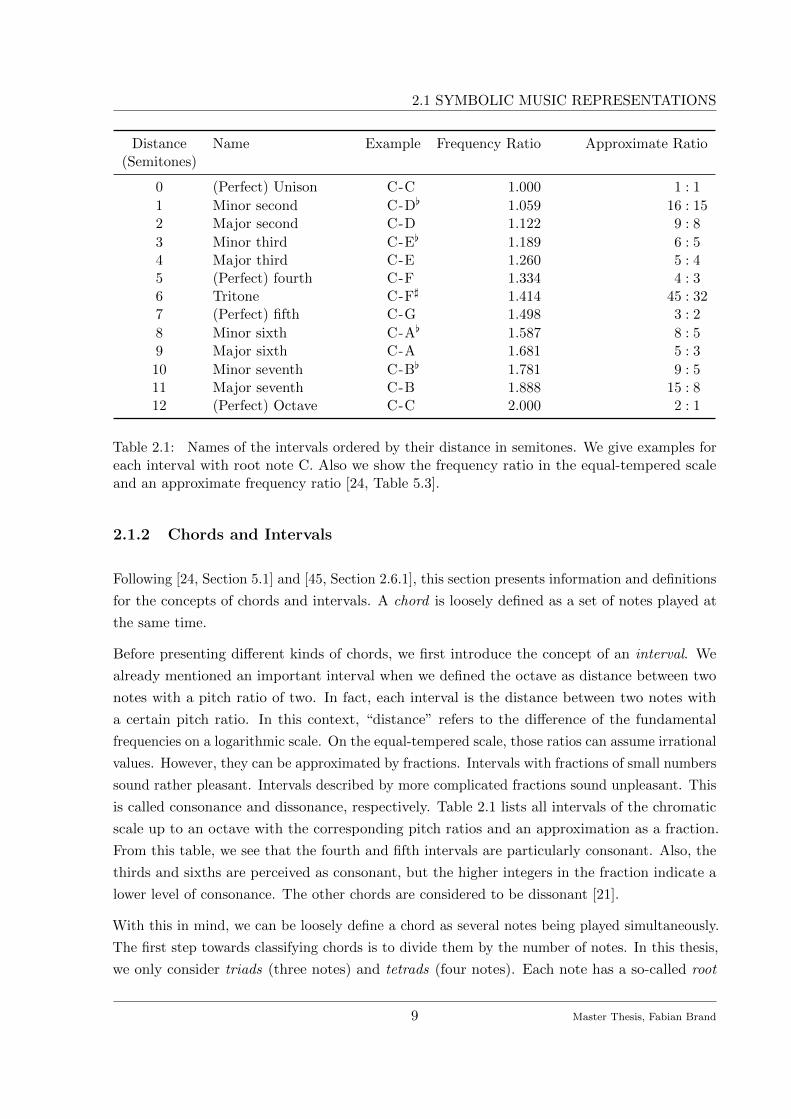
Distance Name Example Frequency Ratio Approximate Ratio(Semitones)
0 (Perfect) Unison C-C 1.000 1 : 1
1 Minor second C-D[ 1.059 16 : 152 Major second C-D 1.122 9 : 8
3 Minor third C-E[ 1.189 6 : 54 Major third C-E 1.260 5 : 45 (Perfect) fourth C-F 1.334 4 : 36 Tritone C-F] 1.414 45 : 327 (Perfect) fifth C-G 1.498 3 : 2
8 Minor sixth C-A[ 1.587 8 : 59 Major sixth C-A 1.681 5 : 3
10 Minor seventh C-B[ 1.781 9 : 511 Major seventh C-B 1.888 15 : 812 (Perfect) Octave C-C 2.000 2 : 1
Table 2.1: Names of the intervals ordered by their distance in semitones. We give examples foreach interval with root note C. Also we show the frequency ratio in the equal-tempered scaleand an approximate frequency ratio [24, Table 5.3].
2.1.2 Chords and Intervals
Following [24, Section 5.1] and [45, Section 2.6.1], this section presents information and definitions
for the concepts of chords and intervals. A chord is loosely defined as a set of notes played at
the same time.
Before presenting different kinds of chords, we first introduce the concept of an interval. We
already mentioned an important interval when we defined the octave as distance between two
notes with a pitch ratio of two. In fact, each interval is the distance between two notes with
a certain pitch ratio. In this context, “distance” refers to the difference of the fundamental
frequencies on a logarithmic scale. On the equal-tempered scale, those ratios can assume irrational
values. However, they can be approximated by fractions. Intervals with fractions of small numbers
sound rather pleasant. Intervals described by more complicated fractions sound unpleasant. This
is called consonance and dissonance, respectively. Table 2.1 lists all intervals of the chromatic
scale up to an octave with the corresponding pitch ratios and an approximation as a fraction.
From this table, we see that the fourth and fifth intervals are particularly consonant. Also, the
thirds and sixths are perceived as consonant, but the higher integers in the fraction indicate a
lower level of consonance. The other chords are considered to be dissonant [21].
With this in mind, we can be loosely define a chord as several notes being played simultaneously.
The first step towards classifying chords is to divide them by the number of notes. In this thesis,
we only consider triads (three notes) and tetrads (four notes). Each note has a so-called root
9 Master Thesis, Fabian Brand

2. BACKGROUND: CHORD RECOGNITION
CM Cm C+ C◦
Figure 2.2: Examples of four triad types in root position.
note, which is the basis of this chord. Often but not always, the root note has the lowest pitch of
the chord. In this case we speak of a chord in root position.
The most important triads in Western music are tertian chords, which consist of notes that can
be stacked in thirds [21], meaning that the interval between two adjacent notes is either a major
or a minor third. The most common triads are the major and minor triads. The major triad
consists of a major third above the root note and a minor third on top of it. The minor triad
consists of a minor third and a major third on top. In both cases, the interval between the lowest
and highest note is a perfect fifth, giving the chords a stable quality. We denote a major triad
with its root pitch class followed by a capital M. For example, the C major triad is written as
CM. The we denote minor triads with a lower-case m, so we abbreviate the C minor triad by
Cm. Figure 2.2 gives an example for both triad types.
A way of mathematically describing a chord is to list the pitch class of all involved notes in a
pitch class set S. We number the pitch classes from 0 to 11 starting with C and ascending in
semitone steps. We can write the pitch class set of CM, which consists of C, E and G, as:
SCM = {0, 4, 7} (2.1)
Another useful representation are chord template vectors. In these twelve-dimensional vectors,
each entry corresponds to one of the pitch classes. If the pitch class is active in the chord, the
corresponding entry is set to 1 otherwise the entry is 0. As an example, we can write the template
vectors of CM and Cm as:
tCM = (1, 0, 0, 0, 1, 0, 0, 1, 0, 0, 0, 0)ᵀ
tCm = (1, 0, 0, 1, 0, 0, 0, 1, 0, 0, 0, 0)ᵀ(2.2)
There are two other possibilities to stack two third intervals by using two major thirds or two
minor thirds. Those chords are called the augmented and diminished triad, respectively. Note
that the interval between the highest and lowest is no longer a perfect interval. The augmented
chord has a minor sixth, also called augmented fifth interval. The diminished chord has a tritone
or diminished fifth interval, which is particularly dissonant. The chords are denoted by “+”
for augmented chords and “◦” for diminished chords. We show note examples of augmented
10 Master Thesis, Fabian Brand

2.1 SYMBOLIC MUSIC REPRESENTATIONS
Figure 2.3: The CM triad in several variations. All shown chords comprise the pitch classes C,E and G, but in different octaves. Even though the musical impressions may be quite differentthey all correspond to the same template vector.
and diminished triads in Figure 2.2 and give the template vectors with the root note C in the
following:
tC+ = (1, 0, 0, 0, 1, 0, 0, 0, 1, 0, 0, 0)ᵀ
tC◦= (1, 0, 0, 1, 0, 0, 1, 0, 0, 0, 0, 0)ᵀ
(2.3)
The template vectors for different root notes can be obtained by cyclically shifting the template
vector of C. The number of shifts equals the distance of the respective pitch classes. For example,
the template vector for Gm can be written as:
tGm = (0, 0, 1, 0, 0, 0, 0,1, 0, 0, 1, 0)ᵀ . (2.4)
For clarity, the entry representing the root note is printed in bold face. By describing a chord
only as a set of pitch classes, there are several different chords corresponding to the same
representation. First, since the octave information is lost, chords played in different octaves are
mapped to the same template vector. Furthermore, inversions—in which the root note is not
the one with the lowest pitch—become indistinguishable. The notes of a chord may even be
distributed over several octaves. Figure 2.3 shows several chords which are all mapped to the
same template vector.
This property is particularly interesting when it comes to symmetric chords, for example the
augmented chord. Without respecting the octave information, it is impossible to distinguish
more than four root notes. Since C+, E+ and G]+ all comprise the pitch classes C, E and G]
they have the same representation, because of the aforementioned enharmonic equivalence. This
will become an issue later on.
This concept can be extended to tetrads or—more specifically—seventh chords, which consist of
a triad and a seventh interval. The chords we use in this thesis consist of three stacked major or
minor thirds. There are eight possibilities, but stacking three major thirds leads to a repetition
of the root pitch class when respecting enharmonic equivalence. Therefore, the chord is an
augmented chord. Hence, seven types of seventh chords remain.1 In Table 2.2, we present the
1There are actually more seventh chords than we described here. However, this is the set we are working with.
11 Master Thesis, Fabian Brand

2. BACKGROUND: CHORD RECOGNITION
Name Notation Template Vector
Major seventh CMmaj7 tCMmaj7= [1, 0, 0, 0, 1, 0, 0, 1, 0, 0, 0, 1]ᵀ
Minor seventh Cm7 tCm7= [1, 0, 0, 1, 0, 0, 0, 1, 0, 0, 1, 0]ᵀ
Dominant seventh CM7 tCM7= [1, 0, 0, 0, 1, 0, 0, 1, 0, 0, 1, 0]ᵀ
Diminished seventh C◦7 tC◦7= [1, 0, 0, 1, 0, 0, 1, 0, 0, 1, 0, 0]ᵀ
Half-dim. seventh Cø7 tCø7= [1, 0, 0, 1, 0, 0, 1, 0, 0, 0, 1, 0]ᵀ
Min. maj. seventh Cmmaj7 tCmmaj7= [1, 0, 0, 1, 0, 0, 0, 1, 0, 0, 0, 1]ᵀ
Aug. maj. seventh C+7 tC+7= [1, 0, 0, 0, 1, 0, 0, 0, 1, 0, 0, 1]ᵀ
Table 2.2: Template vectors of the different seventh chords we use in this thesis.
template vectors of all used seventh chords for reference. When inspecting the diminished seventh
chord, we can see that—similarly to the augmented triad—the template vector is symmetric. In
this case, there are only three distinguishable root notes.
In this section, we gave an overview over the basic building blocks of Western music. We limited
ourselves to concepts which are necessary to follow the technical content of the thesis. For a
more detailed discussion of musical theory, we refer to [45, Chapter 2].
2.2 Feature Representation
In the previous section, we discussed some musical concepts on a symbolic level. Now, we
introduce several ways to represent music recordings in a technical context. This part is based
on [24, Chapter 3.1] with a brief part taken from [24, Chapter 1.3.1].
An audio recording captures the relative air pressure as measured by a microphone which can
be reproduced by a loudspeaker. Typically, 44100 or 22050 samples are recorded per second. A
sampling rate Fs of more than 40000 Hz is sufficient to represent all frequencies audible for humans.
We now want to transform the waveform into a musically meaningful representation with a lower
sampling rate. As a first step, most MIR approaches apply the short-time Fourier transform
(STFT) in order to transform the waveform into a so called spectrogram, which is used to analyze
the predominant frequencies. An extensive discussion of the different kinds of Fourier transforms
and the STFT can be found in [24, Chapter 2]. The STFT splits the signal into small overlapping
windows and transforms each window into the frequency domain. The resulting amplitude vectors
are then concatenated to obtain a two dimensional representation X (n, k) ∈ RN×K , with N and
K as the number of time frames and frequency bins, respectively. This contains information
about the energy of the signal at time frame n ∈ [1 : N ] := {1, 2, . . . , N}, and frequency index
k ∈ [0 : K]. Each value of k corresponds to a frequency Fcoeff(k) = kFsNw
with the STFT window
size Nw.
12 Master Thesis, Fabian Brand

2.2 FEATURE REPRESENTATION
As described in the previous section, the human perception of frequency is logarithmic. Therefore,
we order the frequencies logarithmically. To get a representation close to the musical context, we
bin the frequencies such that they match the pitch scale discussed in Section 2.1. We obtain the
so-called log-frequency spectrogram YLF ∈ RN×128 by summing up all frequency bins close to
the mid frequency of each pitch p ∈ [0 : 127]
YLF (n, p) =∑
k∈Pp(p)
|X (n, k)|2 , (2.5)
where P (p) is the set of all frequency indices k belonging to the pitch p
Pp(p) = {k : Fpitch(p− 0.5) ≤ Fcoeff(k) < Fpitch(p+ 0.5)} , (2.6)
with the center frequency of pitch p
Fpitch(p) = 2(p−69)/12 · 440 Hz. (2.7)
With this definition the note A4 (concert pitch) is assigned to pitch number 69 and the note C4
(middle C) corresponds to pitch number 60. The resulting spectrogram YLF (n, p) captures the
energy of the pitch with index p at time index n.
In many cases—as in chord recognition—we are not interested in the octave of a note. Instead
the pitch class is carrying the relevant information. Therefore, we convert the log-frequency
spectrogram into a pitch class representation, also known as a chromagram [44]. The idea behind
the chromagram C ∈ RN×12 is straightforward as we sum up the energies of all pitches belonging
to the same pitch class. Those are all the pitches with indexes that are congruent modulo 12 to
each other. We define:
C (n, c) =∑
p∈Pc(c)
YLF (n, p) , (2.8)
with Pc(c) = {p ∈ [0 : 127] | p mod 12 = c} and c ∈ [0 : 11]. The matrix C can be interpreted as
a temporal sequence of 12-dimensional vectors x. Those vectors are called chroma vectors or
chroma features. In addition, the chroma features are usually normalized either with respect to
the `1 or the `2 norm. In this thesis, we use the `1 norm. This way the features are invariant
to dynamic changes. To avoid division by zero in frames of silence, which leads to degenerated
features, we use a thresholding procedure. If the total energy of a frame is below a certain
threshold, all entries of the vector are set to 112 . The feature space F of the chroma features
therefore comprises all twelve-dimensional vectors with positive entries that sum up to 1:
F ={x ∈ R12
≥0 : ||x||1 = 1}, (2.9)
with the set of all non-negative real numbers R≥0.
13 Master Thesis, Fabian Brand

2. BACKGROUND: CHORD RECOGNITION
Figure 2.4: Log-frequency spectrogram (a) and chromagram (b) for the first 50 frames of theBach choral example
In Figure 2.4, we show the log-frequency spectrogram and the chroma features of the Bach choral
example. We see that a high value in the spectrogram leads to a high value in the chromagram.
However, we can also see high values in the chromagram, where there is apparent silence in
the spectrogram (e.g. in the beginning of the recording). This is due to the normalization.
This example demonstrates the invariance with respect to changing dynamics. We compute
those features using the publicly available Chroma Toolbox2 [25]. The method for obtaining the
log-frequency spectrogram differs from the introduced STFT method by using elliptic filters to
directly compute the pitch energies.
2www.audiolabs-erlangen.de/resources/MIR/chromatoolbox
14 Master Thesis, Fabian Brand

2.2 FEATURE REPRESENTATION
There are several possibilities how to further enhance the chroma features. One problem of
the described chroma features is that different instruments generate a high dynamic range
in log-frequency spectrograms. If we generate chroma features from such a spectrogram, we
obtain very different chroma feature for different recordings. Especially if we use the features in
classifiers this difference will yield problems [9]. A common method to overcome this problem
is the logarithmic compression, which effectively limits the dynamic range of the spectrogram.
There are several approaches for logarithmic compression found in [9, 24,26]. Cho and Bello [9]
define logarithmic compression as follows:
Y(η)LF (n, p) = log
(1 + η · YLF(n, p)
maxp YLF(n, p)
), (2.10)
with the parameter η, which is typically chosen between 100 and 10000. The obtained spectrogram
is then folded into chroma vectors as described in Eq. 2.8.
Another problem concerns with overtones. A note played by a real world instrument produces
the fundamental frequency of the tone and additional overtones. The frequencies of the overtones
are integer multiples of the fundamental frequency. For example a concert A played on a piano
comprises the frequencies 440 Hz, 880 Hz, 1320 Hz, 1760 Hz, 2200 Hz, . . .. These frequencies
approximately correspond to the pitch classes A, A, E, A and C], respectively3. The spectral power
of each overtone strongly depends on the instrument. In fact, this is one of the characteristics
which give each instrument its unique sound. However, this poses an issue if we are only interested
in the fundamental frequencies. From the example mentioned above, we see that a played note
contributes to more than one pitch class, which makes it considerably harder to get information
about the musical content.
An easy approach is octave suppression. Here, a logarithmic frequency spectrogram is multiplied
with a window function, reducing the energies in the high and low pitches. The underlying
assumption is that the fundamental frequencies are located in the middle of the spectrum. The
high frequencies consist mostly of overtones, whereas the low frequencies usually have a bad
resolution, due to properties of the STFT and the logarithmic binning. Also, the low-frequency
bins a often distorted by a base drum in pop or rock music [9]. In [9] Cho and Bello use a
Gaussian window centered around pitch C4 over the logarithmic frequency axis and compute the
octave suppressed log-frequency spectrogram as
YOSLF (n, p) = YLF(n, p) · exp
(−(p− 60)2
2 · 152
). (2.11)
3Note that the first few overtones are all part of the AM triad. This explains the pleasant sound of majortriads, since all notes are consonant with the natural overtones of the root note.
15 Master Thesis, Fabian Brand

2. BACKGROUND: CHORD RECOGNITION
In [23], Mauch and Dixon propose a more sophisticated approach. The proposed chroma
features, called non-negative least squares (NNLS) chroma, are based on a fundamental frequency
spectrogram, which contains only the fundamental frequencies without the overtones. This
spectrogram is estimated by using an overtone model with geometrically declining amplitudes.
The amplitude of the hth overtone relative to the amplitude of the fundamental frequency
is modeled as sh with the spectral shape parameter 0 ≤ s ≤ 1. We are then dealing with
an optimization problem trying to find the fundamental pitches that—in combination with
the overtone model—best explain the measured spectrogram. The resulting spectrogram is
transformed into chroma features as before. The concept of NNLS chroma was implemented
in a Vamp plug-in4, which can be used in open source software like Sonic Visualizer5 or Sonic
Annotator6. This plug-in also contains a spectral whitening technique, which has a similar effect
as logarithmic compression. In [9] Cho and Bello extensively study the different extensions of
the chroma features and compare them in the context of chord recognition. In the following, we
use NNLS chroma with s = 0.7.
2.3 Template-Based Chord Recognition
In the previous sections, we discussed the theoretical foundations for chord recognition. This
section describes and discusses a straightforward approach for chord recognition based on template
matching. This section is based on [24, Chapter 5.2] and [9]. Chroma-based chord recognition
was initially introduced by Fujishima [14].
In the previous section, we introduced the chroma feature as a music representation capturing
the different pitch classes. We showed that an audio recording can be transformed to a sequence
of twelve-dimensional chroma vectors, which capture the energy of each pitch class. Comparing
this representation to the chord templates defined in Section 2.1, we find conceptual similarities
between both representations. Both vectors describe an energy distribution on the different
pitch classes. The similarity of a chroma vector and chord template can be a measure of the
probability of the chord in this time frame. We define the template-based similarity measure
st
(x, tλ
)between the chroma vector x and the chord template tλ as
st
(x, tλ
)=
〈x|tλ〉||x||1 · ||tλ||1
, (2.12)
where tλ is the template corresponding to the chord λ and 〈·|·〉 denotes the inner product of two
vectors. ||·||1 denotes the `1 norm.
4http://isophonics.net/nnls-chroma5http://www.sonicvisualiser.org6http://www.vamp-plugins.org/sonic-annotator
16 Master Thesis, Fabian Brand

2.3 TEMPLATE-BASED CHORD RECOGNITION
Figure 2.5: Results of template-based chord recognition of the Bach example. The result iscolor-coded: black represents true positives (TP), red false negatives (FN) and blue false positives(FP). Every color except black and white represents an error.
For estimating a chord label, we pick the chord which maximizes this similarity measure:
λ = argmaxλ∈Λ
st
(x, tλ
). (2.13)
Here Λ denotes a set of chords called a chord vocabulary. Usually Λ comprises all 24 major and
minor chords [5, 8, 9, 20]. Figure 2.5 shows an example of template-based chord recognition on
the Bach example. The plot shows a comparison to the ground truth chords. We obtained the
ground truth by manually annotating the recording. For this annotation all chords were mapped
on major and minor triads. This is not always justified, especially when dealing with augmented
and diminished chords. If a chord was classified correctly7 we call it a true positives (TP) and
visualize it in black. If a chord is classified incorrectly, this causes two errors. One error occurs
at the annotated chord, which was not classified correctly. We call that a false negative (FN)
and assign it the color red. Another error occurs at the classified chord which was not annotated.
We call this error a false positive (FP) and display it in blue.
In general, we see that the system recognizes many chords correctly. However, there are also
several errors. We can explain some of them musically, such as the error occurring between
frames 40 and 50. Here, C]m is annotated but EM is detected. Looking in the musical score we
find that actually C]m7
was played. In the annotation, the chord was mapped to C]m but since
C]m7
comprises the pitch classes of both C]m and EM, both results are possible. There are also
other effects which can lead to a misclassification of a chord, such as overtones and the presence
of non-chord notes. This kind of error is usually present for the entire duration of a chord or at
7In reality annotations are not always correct or unambiguous. Nevertheless we call a detected chord thatmatches the annotation “correct”.
17 Master Thesis, Fabian Brand

2. BACKGROUND: CHORD RECOGNITION
Figure 2.6: Results of template-based chord recognition of the Bach example with temporallysmoothed chroma vectors.
least the duration of a note. However, there are many short errors lasting only a few frames.
These errors result from the presence of noise in the signal. We can clearly recognize the errors
since the duration of the detected chords is shorter than of naturally occurring chords, which we
assume to be about one or two seconds. We can prevent that error by smoothing the chroma
features over time before the classification. In Figure 2.6, a moving average with a two-sided
window size of 11 frames was applied to the chromagram before classification. We see that most
of the outliers are gone, but on the other hand, we now suffer from a reduced temporal resolution.
There are more errors at the edges of correctly recognized chords. The overall accuracy was
reduced from 75.9% without smoothing to 73.4% with smoothing. This smoothing approach
does not respect the context of the recording. We introduce a more sophisticated smoothing
technique in the next section.
The accuracy of a chord recognition result is defined as the percentage of correctly estimated
annotated chord frames. This means that we ignore frames without annotated chord for the
calculation. An example for such frames are the frames in the end of the Bach example (n > 500),
where we perceive only silence. This is necessary due to the lack of the “no-chord” label in our
chord model.
At this point, we briefly discuss typical chord confusions. The more common notes two chords
have, the more likely the system will confuse them. Limiting ourselves to the major and minor
chords, each chord has three chords which two common notes. For CM those are Cm, Em and
Am. Note that the mode changes for all confusions. The root notes of the confusion chords are
the original root note, a major third above the root note and a major sixth above the root note.
We can find similar patterns for minor triads.
18 Master Thesis, Fabian Brand
2.3 TEMPLATE-BASED CHORD RECOGNITION
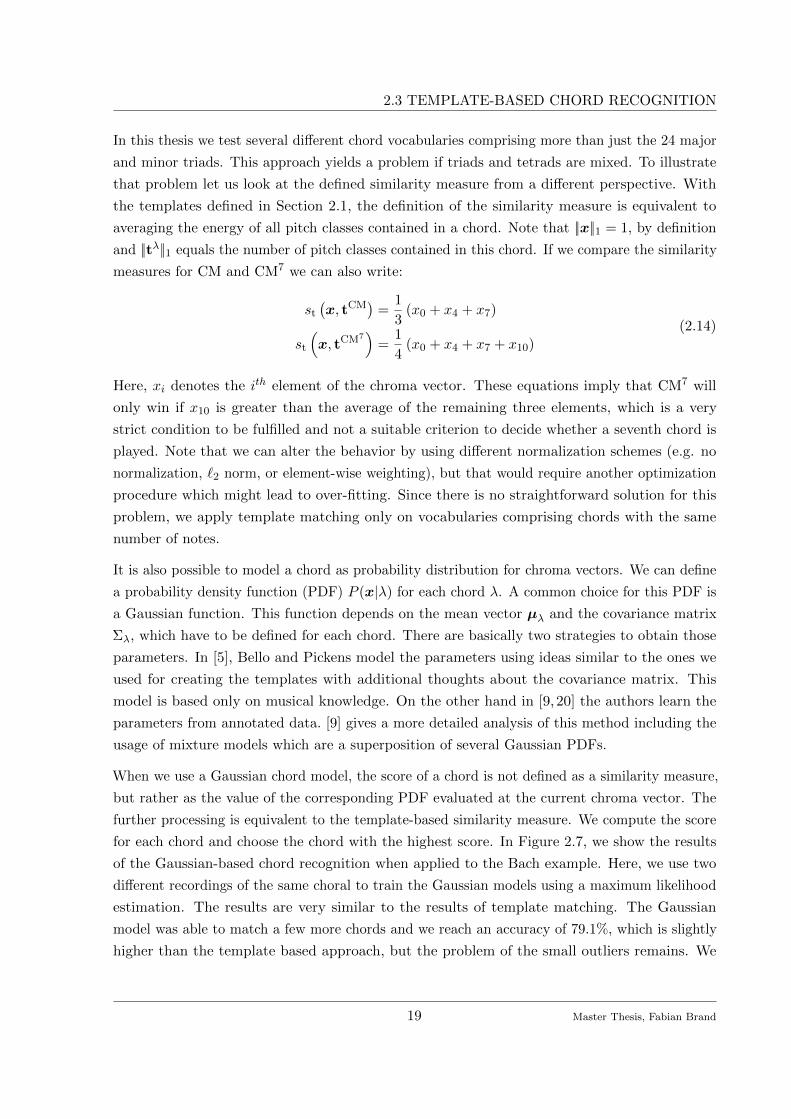
In this thesis we test several different chord vocabularies comprising more than just the 24 major
and minor triads. This approach yields a problem if triads and tetrads are mixed. To illustrate
that problem let us look at the defined similarity measure from a different perspective. With
the templates defined in Section 2.1, the definition of the similarity measure is equivalent to
averaging the energy of all pitch classes contained in a chord. Note that ||x||1 = 1, by definition
and ||tλ||1 equals the number of pitch classes contained in this chord. If we compare the similarity
measures for CM and CM7 we can also write:
st
(x, tCM
)=
1
3(x0 + x4 + x7)
st
(x, tCM7
)=
1
4(x0 + x4 + x7 + x10)
(2.14)
Here, xi denotes the ith element of the chroma vector. These equations imply that CM7 will
only win if x10 is greater than the average of the remaining three elements, which is a very
strict condition to be fulfilled and not a suitable criterion to decide whether a seventh chord is
played. Note that we can alter the behavior by using different normalization schemes (e.g. no
normalization, `2 norm, or element-wise weighting), but that would require another optimization
procedure which might lead to over-fitting. Since there is no straightforward solution for this
problem, we apply template matching only on vocabularies comprising chords with the same
number of notes.
It is also possible to model a chord as probability distribution for chroma vectors. We can define
a probability density function (PDF) P (x|λ) for each chord λ. A common choice for this PDF is
a Gaussian function. This function depends on the mean vector µλ and the covariance matrix
Σλ, which have to be defined for each chord. There are basically two strategies to obtain those
parameters. In [5], Bello and Pickens model the parameters using ideas similar to the ones we
used for creating the templates with additional thoughts about the covariance matrix. This
model is based only on musical knowledge. On the other hand in [9,20] the authors learn the
parameters from annotated data. [9] gives a more detailed analysis of this method including the
usage of mixture models which are a superposition of several Gaussian PDFs.
When we use a Gaussian chord model, the score of a chord is not defined as a similarity measure,
but rather as the value of the corresponding PDF evaluated at the current chroma vector. The
further processing is equivalent to the template-based similarity measure. We compute the score
for each chord and choose the chord with the highest score. In Figure 2.7, we show the results
of the Gaussian-based chord recognition when applied to the Bach example. Here, we use two
different recordings of the same choral to train the Gaussian models using a maximum likelihood
estimation. The results are very similar to the results of template matching. The Gaussian
model was able to match a few more chords and we reach an accuracy of 79.1%, which is slightly
higher than the template based approach, but the problem of the small outliers remains. We
19 Master Thesis, Fabian Brand

2. BACKGROUND: CHORD RECOGNITION
Figure 2.7: Results of the chord recognition with Gaussian chord models.
could not be solve the problem with this approach. The next section introduces a model that
allows context-sensitive smoothing.
2.4 HMM-Based Chord Recognition
This chapter introduces the Hidden Markov Model (HMM), which is widely applied within
mathematics and engineering [6,10,32] and can also be used for chord recognition [36]. An HMM
is a model that describes sequence data by hidden internal states and an observable output
variable. In the first part of this section, we explain the general idea behind the model and show
that it can be useful for chord recognition. In the next part, we show the application to our
problem. The theoretical part is mainly based on [33] and [24, Chapter 5.3].
The HMM is based on the so-called Markov chain. A Markov chain consists of a set A of I
discrete states αi ∈ A, i ∈ [1 : I]. At each time step n, the model is in exactly one state sn ∈ A,
n ∈ [1 : N ], with N as length of the sequence. After each time step, the state changes according
to a probability distribution which only depends on the previous state and neither on the states
before the previous state nor on the specific time instant. This assumption is central in the
theory of Markov chains and HMMs and is called the Markov property. We can write it as:
P (sn=αj |sn−1 =αi, sn−2 =αk, . . .) = P (sn=αj |sn−1 =αi) = aij , (2.15)
where the state transition probability aij ∈ [0, 1] denotes the probability of a transition between
αi and αj . We can summarize the state transition probabilities in the state transition matrix A.
Together with the initial state probabilities ci = P (s1 =αi), which describe the state probabilities
at n = 1, we can compute the probabilities for all states at all times.
20 Master Thesis, Fabian Brand

2.4 HMM-BASED CHORD RECOGNITION
In many applications, the states of a system are not directly observable. Instead, we observe
a variable that depends on the state in a probabilistic sense but is unable to tell us the state
exactly. By hiding the states from the observer and introducing an observation variable on, we
arrive at the Hidden Markov Model. The observation variable on describes the observable output
of the model at time n and follows a random distribution that depends only on the current state.
We define B as the set of all possible observations and the state-dependent emission probability
distribution bi(on) : B → R≥0, which maps the observation space B to the non-negative real
numbers8. We define
bi(on) = P (on|sn=αi) , (2.16)
where x is the observed vector. Overall, the HMM Θ is defined as a tuple containing the set of
states A, the transition matrix A, the set of initial state probabilities C, the set of observations
B and the set of emission probabilities B:
Θ = (A, A,C,B, B) (2.17)
With this in mind, we now apply an HMM to chord recognition. We can use the chords as hidden
states and chroma vectors as observations. We now show how the different aspects of an HMM
are applicable on chord recognition. We first look at the chords, which we model as a Markov
chain. We can split the recording in time frames and assign each frame one chord. The chord
in the next time step depends on the previous chord. This is true since some chords are more
likely to follow each other. For example transitions with fifth intervals between root notes are
more probable than others. The most important transition to consider is the self-transition, i.e.
the probability that the chord does not change. This probability is high compared to the other
probabilities since a chord is usually played for more than one frame. On the other hand, the
probability for a certain chord also depends on chords further in the past, since there are typical
chord sequences in some genres, like the 12 bar blues scheme. However, such a behavior violates
the Markov property and therefore exceeds the model. Therefore the HMM cannot take these
properties into account. As for the initial state probabilities, we typically set them to a uniform
distribution, since we usually have no prior knowledge about the scale or other tonal information
about the recording.
We see that we can model the chords as a Markov chain. Since we do not observe the chord
directly we extend the model to an HMM by adding the chroma vectors x as observations. If the
HMM is in the state of a certain chord, this changes the probability distributions of the chroma
vectors. If the model is in state CM for example, a chroma vector with high energies at C, E and
G has a higher probability than other vectors. In Figure 2.8 we show a toy example of an HMM.
8For a finite number of observations, we can give actual probabilities, which only assumes values between 0 and1. For continuous observations we need to use a probability density function, which can assume all non-negativereal numbers.
21 Master Thesis, Fabian Brand

2. BACKGROUND: CHORD RECOGNITION
(a) (b)
Figure 2.8: Toy example of an HMM describing only three chords. We show a state transitiondiagram with emissions in (a), taken from [24, Figure 5.28a]. We show the state transition matrixin (b). We plot the logarithm of the probabilities for a better visual quality.
The model comprises only three chords and three possible outputs. When we look at the state
transition probabilities, we see that each chord favors a certain chroma vector output, but it
is impossible to be sure about the chord just by looking at the chroma vector. The figure also
shows a plot of the transition matrix in a way we use throughout the thesis. The vertical axis
shows the previous state and the horizontal axis shows the target state.
With these considerations, we obtain a full hidden Markov model describing the chords in
connection with the emissions. We can now reformulate the chord recognition problem as finding
an optimal state sequence given a certain observation sequence. In fact there is a standard
algorithm for solving this problem: the Viterbi algorithm. We explain the algorithm more
thoroughly in Section 3.1. Figure 2.9 gives an example for an estimated chord sequence, which
we computed with the Viterbi algorithm. Comparing the plot to Figures 2.5 and 2.6, there are
less outliers but the edges of the chords are still preserved. The achieved accuracy rises to 83.3%.
However, we still see the same errors as in Figure 2.5 at frames 40 to 50 and 170 to 200. Those
can be explained musically and are hard to avoid due to ambiguities in the chord model.
Now we need to find suitable model parameters A and B. We can train the transition probabilities
using labeled data. In [20], Jiang et al. counted the transitions in a training set to get an
estimate. That way, they can exploit the general musical structure since many songs follow
similar chord patterns. However, in [9], Cho and Bello showed that the main gain of HMM-based
22 Master Thesis, Fabian Brand

2.4 HMM-BASED CHORD RECOGNITION
Figure 2.9: Chord sequence of the Bach example estimated with the Viterbi-algorithm.
chord recognition schemes is the smoothing property caused by a high self-transition probability.
We can exploit the smoothing property by setting the main diagonal to a suitable value and
setting all remaining entries to another, smaller value. In [5], Bello and Pickens propose another
approach, which chooses the different transition probabilities according to the distance in the
circle of fifths. The transition probabilities decrease linearly with higher distances. This captures
some musical properties in a generic way without training. However, this method becomes
more complicated when considering a larger number of chords, therefore in the following, we
only enhance the main diagonal of the state transition probability matrix to achieve smoothing.
Figure 2.10 shows two examples of possible transition matrix, one of the is trained from labeled
data and the other one is modeled with an enhanced main diagonal. The trained matrix shows
also higher probabilities for rising and falling fifth transitions which complies to music theory.
The modeled matrix does not capture such properties.
We can use basic similarity measures as model for the emission probabilities, such as the template
similarity measure st or the value of a Gaussian PDF modeling the chords. That way, we have
two different models. In this thesis we call them “template emission model” and “Gaussian
emission model”. Note that both functions are not PDFs, since their integral over F is not
equal to 1, as would be the case for an actual PDF. However, this is not important in the used
algorithms. In the remainder of the thesis we limit ourselves to template emission models due to
their simplicity and because they do not require training, but yield chord recognition results of
sufficient quality.
This section introduced a powerful tool to jointly model chords and chroma vectors mathematically.
With the HMM it is possible to obtain optimal chord sequences, using context-sensitive smoothing.
We also can get insight in the probabilities for certain chords and chord transition, which we use
in the next chapter.
23 Master Thesis, Fabian Brand

2. BACKGROUND: CHORD RECOGNITION
(a) Trained Transition Matrix (b) Modeled Transition Matrix
Figure 2.10: Two examples of possible transition matrices. We trained the matrix in (a) onannotated Beatles songs and modeled the matrix in (b) by enhancing the main diagonal of anuniform matrix. We display both matrices in the logarithmic domain.
24 Master Thesis, Fabian Brand

3. CHORD TRANSITION FEATURES
Chapter 3
Chord Transition Features
In this chapter, we propose two different kind of chord transition features, which contain
information about the frequencies of different chord transitions. In [45] Weiß proposes chord
transition features and showed that information about chord transitions is useful for several
classification tasks. The features need to be transposition invariant, i.e. invariant to recordings
played in different keys.
In [45] Weiß estimated the chord sequence with the Vamp plugin ”Chordino”1, which uses
the Viterbi algorithm, and counted the transitions. However, there was a hard decision for a
chord sequence involved. Even if two chords have almost the same probability, the system has
to decide for one before further processing. A wrong decision yields two errors, once in the
transition into the chord, once in the transition to the next chord. In this thesis, we propose
a feature extraction scheme that avoids hard decisions, aiming towards robust features with a
high descriptive power. The features should be able to describe chord transitions in a way that
depends only on the musical content and not on the specific recording, which may vary in tempo,
key and instrumentation.
In the following, we propose two analogous transition feature extractors, which both are built
on HMMs. The first one uses the Viterbi algorithm involving hard decisions, the other uses the
Baum–Welch algorithm, which allows for a soft decision approach. The base for both approaches
is a HMM modelling the chords as described in the Section 2.4.
3.1 Viterbi-Based Features
First, we introduce Viterbi-based chord transition features, which involve hard decisions. The
Viterbi algorithm [43] is commonly used to determine the optimal state sequence in an HMM
1http://www.isophonics.net/nnls-chroma
25 Master Thesis, Fabian Brand

3. CHORD TRANSITION FEATURES
Θ when the observation sequence is known. As discussed in the previous chapter, we can use
this algorithm to estimate an optimal chord sequence given a sequence of chroma vectors. In
this section, we introduce an approach which derives chord transition features from the detected
sequence. At first, we introduce the Viterbi algorithm before discussing the feature generation
itself. The following explanation is a summary of [24,33].
The Viterbi algorithm finds an optimal state sequence S = (s1, s2, . . . , sN ), with N being the
length of the sequence, also called path, such that the joint probability of the state sequence
S = (s1, s2, . . . , sN ) and the observation sequence O = (o1,o2, . . . ,oN ) given a model Θ is
maximized:
S = argmaxS
P (O,S|Θ) . (3.1)
This is a hard optimization problem since testing all possible state sequences has a complexity
of O(IN), with I as the number of states. However, the Viterbi algorithm uses dynamic
programming to decrease the complexity to O(I2N
), which is linear in the sequence length N .
The idea behind the algorithm is to iteratively optimize the paths from the beginning of the
sequence up to a certain state. This is done efficiently by using the results of the previous time
step. This is only possible because of the Markov property, since otherwise we would need to look
further back in the path. With the Markov property, however, we can optimize the path step by
step by optimizing sub-sequences. If we add another state to the sub-sequence—which is already
optimized—we only have to check all I2 transitions from the last step to the next. We perform
this procedure iteratively for all time steps n ∈ [2 : N ] until the whole sequence is optimized.
As an input, the Viterbi algorithm needs the observation sequence and the model parameters,
particularly the number of states, the state transition matrix and the emission probability
functions. Additionally, we need an auxiliary variable D (i, n) which captures the probabilities of
the optimized sub-sequences:
D (i, n) = maxs1...sn−1
P (o1 . . .on, s1 . . . sn−1, sn=αi|Θ) . (3.2)
D (i, n) is the joint probability for the best (most probable) state sub-sequence ending in state αi
at time n and the given output sub-sequence (o1,o2, . . . ,on). Here, n ∈ [1 : N ] := {1, 2, . . . , N}is the time index and i ∈ [1 : I] is the state index. We can express the maximum path probability
with the help of D (i,N):
maxS=(s1...sN )
P (S,O|Θ) = maxi∈[1:I]
D (i,N) . (3.3)
We can compute D (i,N) iteratively. The iteration starts by setting
D (i, 1) = P (o1, s1 =αi|Θ) = cibi(o1). (3.4)
26 Master Thesis, Fabian Brand

3.1 VITERBI-BASED FEATURES
To compute D (i, n) for the following frame, consider that we know the maximal path probabilities
to all states of the previous frame. As an intermediate step, we compute the path probability if
for fixed states sn−1 and sn:
maxs1...sn−2
P (o1 . . .on, s1 . . . sn−2, sn−1 =αj , sn=αi|Θ) = D (j, n− 1) · aji · bi(on), (3.5)
with j ∈ [1 : I]. We compute the probability by multiplying the maximum probability to reach
αj in frame n − 1 (given by D (j, n− 1)) with the transition probability from state αj to αi
(given by aji) and the probability that state αi emits on (given by bi(on)). We can derive the
expression using Bayesian inference. By maximizing this expression over sn−1 we obtain the
following formula for D (i, n):
D (i, n) = bi(on) · maxj∈[1:I]
D (j, n− 1) · aji. (3.6)
With this iteration procedure we can compute D (i,N). However, this does not yet solve the
problem since we search the sequence itself, not its probability. Therefore, we need to retrace
our steps to arrive at D (i,N). Algorithmically, we implement the procedure by introducing a
backtracking variable E (i, n) ∈ [1 : I], which saves the states yielding the optimal sequences
corresponding to each time step n and state si. We define it as
E (i, n− 1) = argmaxj∈[1:I]
(D (j, n− 1) · aji) . (3.7)
To apply the backtracking, we define state indices in ∈ [1 : I], such that the sequence S =
αi1αi2 . . . αiN is optimal. Starting with
iN = argmaxj∈[1:I]
D (j,N) , (3.8)
we apply recursion to find the remaining indices:
in = E (in+1, n) . (3.9)
That way we can find the entire optimal sequence:
sn = αin . (3.10)
We can visualize one central step of the Viterbi algorithm using a so-called trellis diagram [2] in
Figure 3.1. A trellis diagram shows the states for each time step as compared to a state transition
diagram as in Figure 2.8. The trellis diagram is useful to visualize paths and time-dependent
variables such as D (i, n). We illustrate the idea of the Viterbi-algorithm by showing a toy
example with three states. As an example we compute D (3, n). To calculate D (3, n) the paths
27 Master Thesis, Fabian Brand

3. CHORD TRANSITION FEATURES
Figure 3.1: Iteration step of the Viterbi algorithm.
from all states in the previous time step are considered. The path with the highest score—the
“survivor” [43]—which we illustrate by a solid line is used to calculate D (3, n). All other paths
are ignored (dashed lines). That way the path is always optimal until time step n. All survivors
are possible parts of the final optimal sequence. The state from which the survivor originates is
saved in the backtracking variable E (i, n− 1). The dashed lines between the time steps n− 2
and n− 1 indicate that there is only one allowed path to each state in time step n− 1. Using
such a diagram, we can obtain the optimal path by retracing the solid lines starting at the state
with the highest probability. Computationally, we use the backtracking variable. Note that not
all survivors are reached, since there are I survivors per time step.
As described in Chapter 2.4, we can now use the Viterbi algorithm to estimate an optimal chord
sequence. For this, we use the chord labels as states and the chroma vectors as observations.
After we obtained an optimal chord sequence as output we visualize the detected chords by a
slightly modified trellis diagram in Figure 3.2. We color those states that are part of the optimal
sequence in black, the other states are white. We can now visualize the transitions by connecting
temporally adjacent states of the optimal sequence. We draw all transitions as red lines. We see
a very stable behavior. The majority of transitions are self-transitions.
We now obtained knowledge about the local chord transitions. We use those features to generate
piece-level features in Chapter 3.4.
3.2 Baum–Welch-Based Features
In the previous chapter, we derived local features describing the chords and chord transitions
based on the Viterbi algorithm. The Viterbi algorithm returns exactly one chord label for each
time step—the information about all other states is discarded. We use the sequence to derive
local chord transition features by “connecting” temporally adjacent chords. In this section,
we introduce another kind of feature which avoids hard decisions. Instead of deriving the
28 Master Thesis, Fabian Brand

3.2 BAUM–WELCH-BASED FEATURES
Figure 3.2: Visualization of the Viterbi-based chord transitions using the Bach example.
transitions from the most probable chord sequence, we compute probabilities for all transitions
in each time step. This information is contained in an intermediate variable of the Baum–Welch
algorithm, which was originally developed for training HMMs [3]. We first describe the Baum–
Welch algorithm already in the context of chord transition estimation. Afterwards, we show
visualization techniques for the obtained local chord transition features.
3.2.1 Baum–Welch Algorithm
Baum proposed the algorithm [3], which is now known as Baum–Welch algorithm, as a method to
re-estimate model parameters in HMMs. The following explanation of the Baum–Welch algorithm
is based on the tutorial of Rabiner [33]. We start with an initial model Θ = (A, A,C,B, B),
specifying all parameters. Furthermore, the algorithm requires an observation sequence O. The
algorithm estimates a new model Θ =(A, A, C,B, B
), which explains the observation sequence
better than the old model, such that
P(O|Θ
)≥ P (O|Θ) . (3.11)
The parameters are estimated from ξn (i, j) which contains the probabilities that a transition
from αi to αj occurs at time step n. This variable is our major interest in the Baum–Welch
algorithm, since it can directly serve as local chord transition feature. The transition probability
is computed using the probabilistic models of HMMs. Formally, we define:
ξn (i, j) = P (sn=αi, sn+1 =αj |O,Θ) , (3.12)
29 Master Thesis, Fabian Brand

3. CHORD TRANSITION FEATURES
vn (i) wn (i)
Initialization v1 (i) = cibi(oi) wN (i) = 1
Iteration vn+1 (j) =[∑I
i=1 vn (i) aij
]bj(on+1) wn (i) =
∑Ij=1 aijbj(on+1)wn+1 (j)
Table 3.1: Equations of the forward and backward algorithm which are used to compute vn (i)and wn (i) respectively.
for n ∈ [1 : N − 1]. To compute the probability for a transition, we need to consider the
probability that we arrive in state sn = αi together with the previous observations. This
probability is captured in the forward variable vn (i):
vn (i) = P (o1o2 . . .on, sn=αi|Θ) . (3.13)
Furthermore, we need the probability that we observe the future observations given that we are
in state sn+1 = αj . We define backward variable wn (i)
wn (i) = P (on+1on+2 . . .oN |sn=αi,Θ) , (3.14)
which represents this probability.
In order to compute vn (i) directly, we have to sum up the joint emission probabilities of all
possible paths ending in sn = αi, which is computationally not feasible. Similarly, to compute
wn (i), we have to sum up the emission probabilities of all paths starting in sn = αi. Using
dynamic programming, we can decrease the computational effort. There are iterative algorithms,
the forward and backward algorithm, to compute both variables efficiently. We state them in
Table 3.1 without further proof. We derive the equations for both algorithms in Appendix A.1
and A.2. Here, we give an intuitive explanation of the forward algorithm. For a more detailed
discussion of both algorithms, please refer to [33].
The forward algorithm exploits the Markov property. Using this property it is computationally
feasible to sum over all possible paths if we know the forward variables of the previous time step.
In turn, those variables contain information about all paths leading to this time step and so on.
Figure 3.3 shows our toy example, this time we compute one step in the forward algorithm. We
see that we have to consider only three different transitions for the computation of vn (3). The
information about the history of the sequence is already contained in the forward variables of
the previous time step. We see, that for capturing the many different paths leading to sn = α3,
only the information drawn in black is needed. This visualizes the low computational complexity.
The intuition behind the forward algorithm is very similar to the Viterbi algorithm. Also the
formulas are analogous, the maximization over all states is simply replaced by a sum over all
30 Master Thesis, Fabian Brand

3.2 BAUM–WELCH-BASED FEATURES
Figure 3.3: This figure shows the calculation of vn (3) out of the forward variables from timestep n− 1. All relevant information is drawn black whereas the rest of the trellis diagram is grey.
states. (Compare the iteration step of the forward algorithm with Eq. 3.6.) The considerations
for the backward algorithm are very similar, with a reversed order.
We compute the forward and backward variables by initializing v1 (i) and wN (i) for all i ∈ [1 : I]
according to the equations in Table 3.1. Afterwards, we apply the iteration step for all n ∈ [1 : N ]
and i ∈ [1 : I]. From those two variables, we can then compute the desired transition probabilities:
ξn (i, j) =vn (i) aijbj(on+1)wn+1 (j)
P (O|Θ). (3.15)
We derive this formula in Appendix A.3 using Bayesian inference and the Markov property. We
can explain the expression for ξn (i, j) intuitively, by considering the contributing components.
The probability for a transition depends on the probabilities of all paths leading to state sn = αi,
captured by vn (i), as well as the probabilities of all paths leading away from state sn+1 = αj which
are represented by P (on+1 . . .oN , sn+1 =αj |Θ) = bj(on+1)wn+1 (j). Also, the prior probability
for a transition from αi to αj , represented by aij must be taken into account. The denominator
P (O|Θ) is merely a normalization factor and is needed for a probabilistic interpretation.2 We
can compute it by:
P (O|Θ) =
I∑i=1
vN (i) . (3.16)
In Figure 3.4 we visualize the components needed to calculate ξn (i, j). Here, we compute the
transition probability of a single transition in our toy example. To calculate the probability
ξn (3, 3) of the transition marked in red, all paths to sn = α3 have to be considered, as well as all
paths leading away from sn+1 = α3. Because of the Markov property, it is sufficient to consider
all paths only up to one time step away. Those path segments are marked in black and are
considered in the forward and backward variable respectively.
2The probability P (O|Θ) is the solution of the so-called evaluation problem as described in [33] and gives theprobability to observe an observation sequence given a model. Using it we can determine which model out ofseveral probably emitted an observation sequence. Solving the evaluation problem is useful for example, in speechrecognition.
31 Master Thesis, Fabian Brand

3. CHORD TRANSITION FEATURES
Figure 3.4: Schematic illustration of the calculation of ξn (i, j), marking all relevant componentsin black.
If we know the probabilities of all transitions originating from αi at time n, we can obtain the
probability that any transition originates from αi at time n, by summing up the probabilities.
This probability is equivalent to the probability of being in state αi at time n. The probability
can be computed from ξn (i, j) by marginalization:
γn (i) = P (sn=αi|O,Θ) =I∑j=1
ξn (i, j) =vn (i)wn (i)
P (O|Θ). (3.17)
We can express γn (i) also just in terms of the forward and backward probabilities. This equation
can be derived from Eq. 3.15 and the iteration step of the backward algorithm3. Even though
ξn (i, j) is only defined for n ∈ [1 : N − 1], this expression holds for all n ∈ [1 : N ]. At this point,
we can stop the algorithm since we have information about the state probabilities and the state
transition probabilities. We can use those probabilities to derive soft chord transition features
and perform a kind of soft chord recognition. We summarize the procedure in Algorithm 3.1.
Here, we use a data structures in form of multi-dimensional arrays V (i, n), W (i, n), Γ (i, n), and
Ξ (i, j, n) instead of the time series variables vn (i), wn (i), γn (i), and ξn (i, j), respectively in
order to assimilate MATLAB code.
For the sake of completeness we briefly discuss the remaining Baum–Welch algorithm. With γn (i)
and ξn (i, j) we can re-estimate the HMM model parameters. By summing up ξn (i, j) and γn (i)
over time, we obtain the expected number of transitions between two states and the expected
number of occurrences of each state. We can re-estimate the new transition probabilities aij by
relating both measures.
aij =expected number of transitions from αi to αj
expected number of transitions from αi=
∑N−1n=1 ξn (i, j)∑N−1n=1 γn (i)
. (3.18)
3This part of the Baum–Welch algorithm is actually called forward backward algorithm. Since it is stronglyconnected to the features derived from the Baum–Welch algorithm and we use it to gain information about themwe still refer to this as Baum–Welch algorithm to avoid confusion.
32 Master Thesis, Fabian Brand

3.2 BAUM–WELCH-BASED FEATURES
Algorithm: Baum–Welch-based chord transition estimationInput: HMM specified by Θ = (A, A,C,B, B)
Observation sequence O = (o1,o2, . . . ,oN )Output: Local state probabilities Γ (i, n)
Local state transition probabilities Ξ (i, j, n)
Procedure:Forward Algorithm: Initialize an (I × N) 2D-array V by V (i, 1) = cibi(o1) fori ∈ [1 : I]. Then, compute in a nested loop for n = 1, . . . , N − 1 and j = 1, . . . , I:
V (j, n+ 1) =[∑I
i=1 V (i, n) aij
]bj(on+1)
Set the normalization factor: ν =[∑I
i=1 V (i,N)]−1
Backward Algorithm: Initialize an (I×N) 2D-array W by W (i,N) = 1 for i ∈ [1 : I].Then, compute in a nested loop for n = N − 1, . . . , 1 and i = 1, . . . , I:
W (i, n) =∑I
j=1 aijbj(on+1)W (j, n+ 1)
Initialize an (I ×N) 2D-array Γ and setΓ (i, n) = ν · V (i, n)W (i, n)
Initialize an (I × I ×N) 3D-array Ξ and setΞ (i, j, n) = ν · V (i, n) aijbj(on+1)W (j, n+ 1)
Return: Γ (i, n) and Ξ (i, j, n)
Algorithm 3.1: Baum–Welch-based chord transition estimation
We can find new estimations for the initial state probabilities ci by:
ci = expected number of times in state αi at time n =
= γ1 (i) .(3.19)
The re-estimation of the emission probability functions depends on the used probabilistic model.
For a Gaussian model, we can re-estimate mean vector and covariance matrix as follows:
µi =
∑Nn=1 γn (i)on∑Nn=1 γn (i)
(3.20)
Σi =
∑Nn=1 γn (i) (on − µi) (on − µi)
ᵀ∑Nn=1 γn (i)
, (3.21)
which is a straightforward way of estimating Gaussian models. In HMM training applications,
we initialize the parameters either randomly or by an educated guess. Afterwards, we perform
the algorithm iteratively, each time with an updated model until the model converges. In this
33 Master Thesis, Fabian Brand

3. CHORD TRANSITION FEATURES
thesis, however, we do not use the Baum–Welch algorithm for training, which is why we do not
cover the training step in detail. Here, we use the algorithm for soft-decision chord recognition
and the corresponding transition estimation. We refer to [33] for further information about the
Baum–Welch algorithm and its application on HMM training.
3.2.2 Visualization Techniques
To use the Baum–Welch algorithm for chord estimation, we initialize the HMM in the same way as
for the Viterbi-algorithm. Afterwards, we use the algorithm to compute local state probabilities
γn (i) and state transition probabilities ξn (i, j). We can visualize these probabilities similar to
Figure 3.2 by connecting all states with red lines representing the respective transitions. Instead
of coloring only one state per time frame in black, we now color all states with a gray value
indicating the probability of being in that state. A darker tone represents a higher probability.
Also, since there is now more than one possible transition at each time step, we have to plot the
transition according to the probabilities as well. In a first approach, we plot every transition with
a probability exceeding a certain threshold. The transparency of the line indicates the probability
of the respective transition. A more intense red color refers to a high transition probability. In
order to properly show the chord transitions, it is necessary to ignore the self-transitions, since
they are much more probable and would visually suppress the other transitions. We show the
result in Figure 3.5a. We see that the plot is not easily readable. This is because the differences
between the values are too small to be captured by such a color map. There are many chords
with similar, high probabilities, e.g. between EM and C]m, which share two common notes. In
this case we see that the transitions EM→ C]m and Em→ C]M are strong in all frames where
both chords are present. This is an artifact of the Baum–Welch algorithm and cannot be avoided.
The transitions going back and forth between states create a symmetric, lattice-like structure.
While those transitions may have musical reasons, they do not describe relevant harmonic change
in the recording. On occasions where the harmonic content changes, we observe more directed
transitions, which are visually covered by the noise-like transitions.
In oder to visualize the harmonic changes, we need to find an algorithm which enhances the
musically relevant, directed transitions, and suppresses the lattice-like “noise floor”. We have
three types of transitions: The self-transitions, which have the highest probabilities, the noise-
like transitions, which have the lowest probabilities, and the musically relevant probabilities.
We assume that those transitions stand out by slightly higher probabilities. Filtering out the
probabilities that stand out from the noise is a complicated problem for multiple reasons. A
major issue is that we deal with normalized matrices. Because of the normalization, the value
of each element is dependent on all other elements. As a result, the probability ranges of the
small value of ρtioned transitions types vary from frame to frame. We also do not know how
many transitions we want to enhance since there might be more than one transition of interest.
34 Master Thesis, Fabian Brand
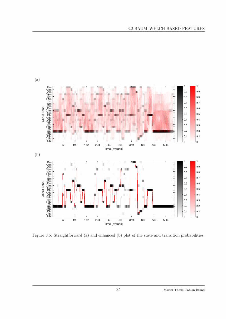
3.2 BAUM–WELCH-BASED FEATURES
(a)
(b)
Figure 3.5: Straightforward (a) and enhanced (b) plot of the state and transition probabilities.
35 Master Thesis, Fabian Brand

3. CHORD TRANSITION FEATURES
Since we know which matrix elements describe the self-transitions, we can discard them, but
distinguishing the other types of transitions is harder. It is not sufficient to raise the threshold,
since the scales differ between the time frames. A way to circumvent that problem is the so-called
softmax function. This function enhances the higher values of a given set while suppressing the
lower ones. We define the softmax function for a matrix X ∈ RM×N as follows:
softmaxη (X) =exp (ηX)∑M
m=1
∑Nn=1 exp (ηX (m,n))
, (3.22)
where exp(·) is the element-wise exponential function and η ∈ R>0 is a parameter determining
the “softness” of the function. A smaller η corresponds to a softer maximization. If we apply
the softmax function on the transition probabilities of each time frame—after deleting the
self-transition probabilities—we enhance the highest probabilities in a flexible way. However, if
there is no value standing out from the noise, the function enhances the highest value, which is
part of the noise.
At this point we see that the complexity of the rescaling task is too high for a conventional
approach like a single softmax rescaling. We therefore introduce an empirically found algorithm:
the double-softmax rescaling. As the name indicates, the algorithm employs two consecutive
softmax functions. At first, we apply the softmax function with a small η1 on all transition
probabilities of one frame, including the self-transition probabilities. Since there is usually at least
one high self-transition probability, this leads to a compression of the remaining probabilities.
Afterwards, we set all self-transition probabilities to zero, before we apply another softmax
function with a high η2 on the resulting matrix. This enhances the highest of the remaining
off-diagonal probabilities. We demonstrate the functionality of the double-softmax rescaling in
Figure 3.6. For this figure we plot all entries of the transition probability matrix for each time
frame in the logarithmic domain. That way, we can see the distribution of the probabilities for
each frame. We indicate the positions of the annotated chord changes by vertical blue lines. In
the first figure, we plot the distribution as obtained by the Baum-Welch algorithm. We color
the self-transition probabilities in red and the other transition probabilities in black. We see
that we have one high self-transition probability in each frame, which corresponds to the chord
with the highest probability. When we look at the other transitions we see a “noise floor” with
several outliers. However, there are many outliers—also in frames without annotated chord
transitions—and we cannot be sure how many of them are musically relevant. In the second
plot, we show the values after the first softmax function. We see that all off-diagonal transition
probabilities are strongly compressed and follow a line that is inverse to the sequence of highest
self-transition probabilities. I.e. if there is one high self-transition probability, the values of the
other transitions are smaller. This is a typical behavior of normalization within the softmax
function. We now take a closer look at the other transitions in the third plot by zooming in
the y-axis. We observe outliers only in a few frames now and also the number of the outliers
36 Master Thesis, Fabian Brand

3.2 BAUM–WELCH-BASED FEATURES
(a) No Rescaling
(b) After the First Softmax
(c) After the First Softmax (Zoomed)
(d) After the Second Softmax
Figure 3.6: Distribution of the transition probabilities for each frame. The blue lines indicateannotated chord transitions.
37 Master Thesis, Fabian Brand

3. CHORD TRANSITION FEATURES
Algorithm: Double-Softmax RescalingInput: Temporal sequence of N − 1 state transition matrices ξn (i, j)
Softmax parameters η1, η2
Output: Temporal sequence of N − 1 state transition matrices ξn (i, j) withsuppressed lattice structure
Procedure:In a loop over all time steps n ∈ [1 : N − 1]:
Initialize a (I × I) matrix Ξ with Ξ (i, j) = ξn (i, j)Set Ξ = softmaxη1 (Ξ)Set Ξ (i, i) = 0 for all i ∈ [1 : I]Set Ξ = softmaxη2 (Ξ)Replace ξn (i, j) with Ξ (i, j) for all i, j ∈ [1 : I]
Return: ξn (i, j)
Algorithm 3.2: Double-softmax rescaling algorithm for the suppression of the lattice structure.
is considerably smaller than before. We see that the outliers match the annotated transitions
to some extent. The values in most frames are now strongly suppressed. The second softmax
enhances those outliers, such that only a few strong transitions remain. If the values are too
close to each other or too small, the second softmax does not enhance these transitions. We show
the resulting distribution after the whole procedure in the fourth plot. We clearly see the noise
floor on the bottom and only a few transitions which have a value higher than 0.01. We can find
those transitions mostly around the positions of the annotated chord changes.
We now plot those values instead of the original probabilities in our trellis diagram in Figure 3.5b.
We empirically chose the parameters η1 = 10 and η2 = 10000. Additionally, we apply a single
softmax (η = 10) on all state probabilities of each time frame. We see that we succeed in
suppressing the lattice structure and that the remaining transition are in fact the transitions
which connect the most probable states. In areas where the state is uncertain, we see transitions
to both states. A good example is around frame 420 where we see transitions from EM to
both BM and Bm. On the other hand, some transitions are not visible anymore since the state
changes only gradually. As an example we look at the frames around time step 350, where the
detected chord changes slowly from BM to Bm. Here, the transition BM→ Bm was spread over
several frames, so that the individual transitions are not strong enough to be enhanced. However,
even though the double-softmax procedure yields good visual results, the tuning of the softmax
parameters is difficult and depends on the used HMM parameters and the data.
In summary, the enhancement algorithm consists of three steps, which we subsequently apply on
all individual matrices ξn (i, j) for each time step n ∈ [1 : N ]. For a compact explanation, see
the box Algorithm 3.2.
38 Master Thesis, Fabian Brand

3.3 COMPARISON AND EVALUATION
3.3 Comparison and Evaluation
In the following, we compare the Viterbi-based and the Baum–Welch-based local chord transition
features. We do not have a quality measure for local transition features available, so we compare
the transitions qualitatively. However, since both feature types are based on a chord recognition
scheme using HMMs, we can quantitatively compare the performance of both algorithms in a
chord recognition scenario.
3.3.1 Influence of the Self-Transition Probability
As a first experiment, we analyze the HMM parameters. In Chapter 2.4, we introduce the state
transition matrix A. We show that we can model the matrix with a uniform matrix of which we
enhance the main diagonal. Such a matrix depends on only one parameter, which describes the
ratio between the main diagonal elements and the off diagonal elements. In [9], Cho and Bello
defined such a parameter. However, we found that this definition has disadvantages when we
compare models with different numbers of states since the self-transition probability depends on
the number of states in the HMM. We propose a different parameter ρ which directly defines the
self-transition probability. We assume that the smoothing properties stay the same even if we
use chord vocabularies of different sizes and, therefore, self-transitions matrices with different
sizes. In [33], Rabiner states that the average duration of a state in a Markov chain depends
only on the self-transition probability of that state. Since the smoothing property is connected
with the average state duration, this result supports our parameter definition. We define the
state transition probabilities as follows:
aij =
ρ if i = j
1−ρI−1 if i 6= j
, (3.23)
with the size of the chord vocabulary I and 0 ≤ ρ ≤ 1. In the context of chord recognition,
a higher choice of ρ leads to a longer average chord duration. Therefore, we obtain a more
stable result. To get a rough idea of the influence, we show the results of the chord recognition
for three selected values of ρ ∈ {0.025, 0.2, 0.5} in Figure 3.7. In this experiment we use the
Viterbi algorithm. For ρ = 0.025, the chord changes very often, we speak of over-segmentation.
Apparently, the smoothing is not strong enough. Nevertheless, for ρ = 0.5, the algorithm misses
several transitions and the smoothing is too strong. This is called under-segmentation. The
value of ρ = 0.2 yields the best of the shown results. We show similar plots for the Baum–Welch
algorithm in Appendix B.1.
We see that ρ has to be tuned carefully, since it influences the results greatly. Therefore we
systematically examine the influence of ρ on a larger database. For this purpose, we use the
39 Master Thesis, Fabian Brand

3. CHORD TRANSITION FEATURES
(a) ρ = 0.025
(b) ρ = 0.2
(c) ρ = 0.5
Figure 3.7: Viterbi-based chord recognition of the Bach example. We use different ρ to modelthe chord transition probabilities.
40 Master Thesis, Fabian Brand

3.3 COMPARISON AND EVALUATION
Figure 3.8: The accuracy of the chord recognition as function of ρ. The experiment was performedon the Beatles dataset using either the Baum–Welch algorithm or the Viterbi algorithm. Thevertical line at ρ = 1
24 marks the point where all transitions have equal probability.
Beatles dataset. It comprises 180 recordings of Beatles songs from the 10 studio albums. Detailed
chord annotations for all songs are publicly available [22]. The dataset is widely used for
benchmarking chord recognition systems within the MIR community [20]. To compare the results,
we perform HMM-based chord recognition on all songs and compute the accuracy by comparing
the result with the annotated ground truth. We define the accuracy as the ratio of correctly
classified frames. Since our chord model does not contain a “no-chord” symbol, we discard all
frames which were annotated with “no-chord”. For the experiment, we reduce all annotated
chords to the chord vocabulary of major and minor triads. We map each chord with a major
third as first interval to the respective major triad and each chord that starts with a minor third
to the respective minor triad. This is not always justified musically, especially when we deal with
augmented and diminished chords, but is common practice [20]. The accuracy is then averaged
over all songs. The result is used as a quality measure for the tested chord recognition system.
For the evaluation of the Viterbi algorithm, we can compare the output sequence directly with
the annotation. The Baum–Welch algorithm does not generate such a sequence. Instead, we use
γn (i) and choose the chord for which γn (i) is maximal in each time frame
sn = argmaxsn
P (sn, O|Θ) = argmaxαi
γn (i) . (3.24)
We perform the described experiment with different values of ρ. Figure 3.8 shows the average
chord recognition accuracy over all songs as a function of ρ. We see that the two algorithms
show different behaviors. In particular, the optimal value of ρ for the Baum–Welch algorithm
is higher than the optimal value of ρ value of the Viterbi algorithm. Since the Baum–Welch
algorithm does not optimize the path probability but rather the individual state probability,
41 Master Thesis, Fabian Brand

3. CHORD TRANSITION FEATURES
the algorithm allows other paths to enhance the probabilities of single states and is therefore
less “strict” than the Viterbi algorithm, which optimizes the entire sequence. As a result, to
obtain the same smoothing effect, we have to choose a higher self-transition probability for the
Baum–Welch algorithm, which explains the different locations of the maximums.
However, we have to be careful when interpreting this result. The chord annotation is not unique,
in particular with respect to the segmentation. In [24, Figure 5.16], Muller gives an example,
how the song “Let it be” can be annotated by different music experts. If we fit the self-transition
probability to an annotation which is highly segmented, the resulting optimal value of ρ will
probably be smaller than a value of ρ fitted to an annotation with coarse segmentation.
Another noteworthy observation is the saturation of the accuracy for the Viterbi algorithm.
For ρ < 0.025 the accuracy does not depend on ρ anymore. In this region, the self-transition
probability is smaller than the other transitions, it is therefore “cheaper” to switch the state
rather than to stay in the state. The Viterbi algorithm is therefore forced to change the state
often in order to optimize the joint probability of the sequence. At a certain point, the chord
changes in (nearly) every time step since staying in a chord is less probable then switching back
and forth to the second most probable chord. Further decreasing the self-transition probability
does not change that behavior, since no self-transitions exist anymore. Also, in the case of very
small ρ, the Baum–Welch algorithm allows other paths to enhance the probability of a state. For
a demonstration of this behavior, see Appendix B.1
The vertical line in Figure 3.8 marks the point where ρ = 124 and thus, all transition probabilities
are equal. The output only depends on the emission probabilities, since the model now does
not inherently prefer one path to any other. In other words, we perform template matching.
Therefore, the result does not depend on the algorithm anymore.
In general, the results from Figure 3.8 are consistent with the intuition we gained from Figure 3.7.
There exists an optimal value for ρ, which is used as a default value for the future experiments.
We set ρ = 0.3 for the Viterbi algorithm and ρ = 0.75 for the Baum–Welch algorithm. We refer
to those values as “standard ρ”. We see, that in these maximums the average accuracy is almost
equal. We can conclude that in the scenario of chord recognition, none of the algorithms is better
than the other. However, we see that the Viterbi algorithm is less sensitive on ρ and has a lower
complexity than the Baum–Welch algorithm. Therefore, if we need only a discrete sequence of
chords, the Viterbi algorithm should be preferred. However, if we are interested in a soft-decision
output, we need to use the Baum–Welch algorithm.
We now use the obtained parameters to examine the Bach choral with both algorithms. We need
to keep in mind that the parameter ρ was fitted on pop music, while we apply it on classical
music. Since the two styles are very different the parameter might not be suitable. We show the
result in Figure 3.9. There is not much difference when we look at the detected chords. Also, the
42 Master Thesis, Fabian Brand

3.3 COMPARISON AND EVALUATION
accuracy is similar with 71.2% for the Viterbi algorithm and 74.8% for Baum–Welch algorithm.
The plot of the Baum–Welch result shows the probability that a chord is played at each time
step. We use a softmax with η = 10 on the state probabilities to visually enhance the plot. While
we see some time frames where the probability is almost one (e.g. frames 400–450), there are also
several frames where two or more chords have similar probabilities. This is the case around time
frame 50. There is a high probability both for F]m and AM. This means that the algorithm
was not sure about the played chord. In the score we see that actually the minor seventh chord
F]m7
was played. In this special scenario, it is therefore possible to gain knowledge exceeding
the model, since F]m7, which is not part of the used chord vocabulary, comprises pitch classes of
both detected chords. This way, we are able to detect some seventh chords types. The Viterbi
algorithm only detects F]m, which is actually correct in the sense of the annotation, without
giving a hint about the seventh chord.
3.3.2 Context-Sensitive Smoothing
The reason why we used HMMs in the first place was the context-sensitive smoothing. We argued
that we can achieve a result where outliers are smoothed but sharp edges could be preserved
at clear chord boundaries. To validate this theory, we perform a smoothed chord recognition
in two ways: once by smoothing the chroma vectors with a moving average filter (window size
of 21 frames) and a subsequent template matching (compare Section 2.3) and once with the
Baum–Welch algorithm (ρ = 0.97). We choose the parameters empirically to obtain strong but
similar smoothing. In both cases, the smoothing is much stronger than needed, but it helps
us to observe the general smoothing behavior of both approaches. Figure 3.10 compares both
algorithms. To get a more detailed view on the transitions, we plot only the first 150 frames. We
show the frame-wise chord probabilities. In the first case we apply a softmax (η = 150) on the
state probabilities to visualize the differences better. We see that the amount of smoothing is
too high in both cases, but the Baum–Welch algorithm manages to obtain sharp edges and to
precisely locate the chord transitions. An example can be found around frame 60. Even though
the previous chord was smoothed too much, the transition to the next chord is very sudden and
at the correct time. On the other hand, a simple smoothing of the chroma vectors yields a very
smooth and inaccurate transition. Around frame 130 we see that the Baum–Welch algorithm
classifies the chord falsely by extending the previous chord too long. However we still obtain a
sharp edge on the transition to the next chord. This scenario visualizes the context-sensitive
smoothing we can achieve with HMMs.
43 Master Thesis, Fabian Brand

3. CHORD TRANSITION FEATURES
Figure 3.9: Comparison of the recognized chords when using (b) the Viterbi and (c) the Baum–Welch algorithm with standard ρ. The score of the fist part of the choral is shown in (a).
44 Master Thesis, Fabian Brand

3.3 COMPARISON AND EVALUATION
(a)
(b)
Figure 3.10: Chord recognition of the Bach example with strong smoothing. As smoothingalgorithm we use (a) a moving average of the chroma vectors and (b) the Baum–Welch algorithm.
45 Master Thesis, Fabian Brand

3. CHORD TRANSITION FEATURES
3.3.3 Local Chord Transition Features
As a next step, we analyze the chord transitions computed with the Viterbi and the Baum–
Welch algorithm. In particular, we look at the transitions around the small value of ρtioned
seventh chord. In Figure 3.11, we show the chord transitions for the frames 40–59. The Viterbi
algorithm yields only two transitions, whereas the Baum–Welch algorithm shows several. Not all
of them describe harmonic changes. First of all, we see the expected transitions EM→ AM and
EM → F]m (frame 40–46). We see transitions in the other direction when the chord changes
back to EM (frame 50–55). The transitions are spread over several frames. This indicates, that a
transition can occur at each of those frames. We see, that the probability of the previous chord
decreases as the probability of the next chord increases. At the same time, we see transitions
from EM→ G]m and back again. This is due to a confusion between EM and G]m, which share
two notes. The same is true for Em and C]m. There are also several other chord transitions
visible. It is not immediately clear why the corresponding chords occur. We can see those
transitions as an artifact. The strength of the transitions contains some information about
overtones and therefore relates to timbre. We see that we were not able to completely eliminate
timbral content. On the other hand, the confusions allow for conclusions about the tonal content.
For example, if only a fifth interval is played, this is usually mapped to the respective major
chord due to the overtone structure. However, since no third is present, the confusion chords
(and the corresponding transitions) except the major-minor confusion probably have only low
probabilities. We can argue that those transitions do not have a clear semantic meaning anymore.
Using the double softmax rescaling introduced in the previous section we can suppress many
transitions as shown in Figure 3.11(c). Here, only the transitions which relate to harmonic
changes remain. We see the transitions from EM to both possible chords AM and F]m, and back.
The plot only shows transitions which correspond to harmonic change but is still respecting that
there might be more than one possible chord.
3.4 Piece-Level Chord Transition Features
In the previous sections, we discuss two different ways of extracting local information about
chord transitions. The Viterbi algorithm yields an optimal state sequence from which we derive
the local transitions. The Baum–Welch algorithm produces transition probabilities for each time
frame.
46 Master Thesis, Fabian Brand

3.4 PIECE-LEVEL CHORD TRANSITION FEATURES
(a) Viterbi
(b) Baum–Welch
(c) Baum–Welch (Double-Softmax)
Figure 3.11: Comparison of the chord transitions when using (a) the Viterbi and (b) theBaum–Welch algorithm with standard ρ. In (c) we show chord transitions computed with theBaum–Welch algorithm after a double-softmax rescaling.
47 Master Thesis, Fabian Brand

3. CHORD TRANSITION FEATURES
3.4.1 Feature Aggregation
In this section, we explain the aggregation algorithm which we use to aggregate the local chord
transition features into global piece-level features, which describe a whole recording instead of
single time instances. At first, we are interested in the relative frequency of occurrence of each
chord transition. We define the variable awij that describes the average probability of a transition
from λi to λj :
awij =
1
N − 1
N−1∑n=1
P (sn=λi, sn+1 =λj) . (3.25)
We call awij weighted chord transition probabilities. The name is based on the state transition
probabilities aij defined for an HMM. We can interpret awij as a kind of state transition probability4
which is weighted with the probability of occurrence of the previous chord. As a consequence, we
haveI∑i=1
I∑j=1
awij = 1, (3.26)
as opposed to,I∑i=1
aij = 1 ∀j ∈ [1 : I]. (3.27)
The main difference is that aij is a conditional probability and awij is a joint probability. We
denote the matrix comprising all weighted chord transition probabilities as Aw.
Starting from the optimal chord sequence obtained from the Viterbi algorithm, we can count the
transitions and set:
awij =
Number of transitions from αi to αjTotal number of transitions
. (3.28)
We need to use a different approach when we use the Baum–Welch algorithm. We obtain the
Baum–Welch-based chord transition probabilities awij by averaging the local transition probabilities
over all N − 1 pairs of neighboring time steps. We can compute the chord transition matrix
directly by:
Awij =
1
N − 1
N−1∑n=1
ξn (i, j) . (3.29)
From this point on, the procedure does not depend on the chord transition estimation algorithm
anymore. Aw contains piece-level information about relative chord transition frequencies, which
we could use as a feature already. However, it is not robust enough against different versions,
since it contains more information than needed. As we mention in the introduction of this
chapter, the feature should be invariant under key and tempo changes. Therefore, we discard all
information about those two measures. The chord transition matrix contains implicit information
4For the Viterbi-based features, this is actually a relative frequency rather than a probability.
48 Master Thesis, Fabian Brand

3.4 PIECE-LEVEL CHORD TRANSITION FEATURES
about the key of the recording, since certain chords are preferred in certain keys. For example,
a recording in the key of C major most likely contains the CM triad more often than the C]M
triad. This is also reflected in the chord transition probabilities. We eliminate the influence
of the key by performing a suitable transform to make the transitions transposition invariant
(TPI), similar as shown in [24, Chapter 5.3.4.2]. We call this procedure the TPI transform. In
the end, a transition from a chord should be independent from the root note of that chord. Since
we deal with different chord types, we have to treat transitions between chord types separately.
To achieve this, the matrix is split into sub-matrices such that each sub-matrix contains only
transitions from one chord type to another chord type. In the case of only major and minor
triads, this results in four sub-matrices (major → major, major → minor, minor → major and
minor → minor). For more chord types, the number of sub-matrices increases accordingly. Also,
note that—since there are only four distinct augmented chords—those sub-matrices may also be
of non-square shape. We transform the sub-matrices separately by averaging over all cyclically
shifted versions. Let X be an arbitrary sub-matrix. Then we can write:
XTPIij =
1
12
11∑l=0
X(i+l) mod 12,(j+l) mod 12. (3.30)
Afterwards, we rebuild the matrix ATPI from the sub-matrices XTPI. That way an entry in the
matrix no longer refers to a transition between two specific chords. Rather, each entry describes
a transition specified by an interval between root notes and a change of chord type. For example,
aw1,5 is the probability of a transition from CM to EM, whereas aTPI
1,5 denotes the probability of
a transition from an arbitrary major chord to another major chord, where the respective root
notes have an interval of four semitones upwards. This way we obtain transposition invariance of
our features.
In the matrix ATPI, the self-transition frequencies depend on the tempo of the recording. The
self-transition probabilities might also contain valuable information about the recording but
this is not connected to the harmonic content. Therefore we discard their effect by setting all
elements on the main diagonals of the local transition matrices to zero and re-normalizing the
matrices, such that the overall sum is one again. That way we assure that the tempo has no
influence on the features. After the modifications, the matrix is now highly redundant. We need
to discard several entries. First, we only need one column of each chord-type sub-matrix, because
of the transposition invariance. Also we need to discard the self-transition probabilities, which
are always zero and therefore contain no information. In the end, we use only a small subset of
the matrix, which comprises all independent and relevant values as feature.
In Figure 3.12, we show the whole process of the feature generation using the Bach example. For
this example, we use the Viterbi algorithm since the results are visually better understandable.
At first, we see a chord estimation result with the respective chord transitions shown as red
49 Master Thesis, Fabian Brand

3. CHORD TRANSITION FEATURES
(a) Estimated states and transitions
(b) Chord transition matrix Aw (c) TPI chord transition matrix ATPI
Figure 3.12: The Viterbi-based feature generating process performed on the Bach example. (a)shows the estimated state sequence and the corresponding state transition. (b) depicts the thechord transition matrix and (c) shows the TPI transition matrix without the main diagonalelements. The marked elements are statistically independent and serve as feature vector. Wedisplay all matrices after logarithmic compression (η = 1000, similar to Equation 2.10).
50 Master Thesis, Fabian Brand

3.4 PIECE-LEVEL CHORD TRANSITION FEATURES
lines between the chords. By averaging the transitions over time, we arrive at the depicted
chord transition matrix, see Figure 3.12b. We see that the matrix is sparse which shows that
there are only few distinct types of transitions detected. The biggest values occur on the main
diagonal, which contains the self-transition probabilities. The values on the main diagonal are a
measure for the time the respective chords are played. We see that among the self-transitions,
the chords EM, and BM have the highest self-transition probabilities, which is consistent with
the recognized chords. For clarity, the plot is divided into four sub-matrices which separate
transitions between pairs of chord types (black lines). For the next matrix, we perform the TPI
transform and set the self-transition probabilities to zero. We see that the elements on each
diagonal of the sub-matrices are now equal. Therefore, we have a high redundancy in this matrix.
The entries marked with a red frame show the relevant information which is not redundant.
Therefore, we select those entries for the final feature vector. That way, we obtain a feature
vector that should have the desired properties of invariance against tempo and key.
3.4.2 Influence of Double-Softmax Rescaling
In Figure 3.13 a and b, we show the resulting matrices Aw and ATPI for the Baum–Welch
algorithm. Here, we directly applied the aggregation algorithm on ξn (i, j). We see, that Aw is
not sparse anymore as opposed to the Viterbi algorithm. For the most probable chord (EM) we
observe that both transitions from and to this chord have a high probability. We see that the
main diagonal still has the highest values. After the TPI transform we have strong diagonal
structures. We see high values at rising and falling fifth transitions (e.g. CM → GM and
CM → FM, respectively), which is similar to observations in [45]. However, we also see high
values at transitions that we often find in the aforementioned lattice-structure (e.g. CM→ Cm
and CM→ Em, compare Section 3.2.2), which are sometimes higher than transitions like the
CM→ Gm transition class, which we find in the estimated chord sequence and therefore assume
to contain information about the harmonic progressions.
Previously we achieved good visual results by applying a double-softmax rescaling on ξn (i, j). We
were able to suppress noise-like transitions thoroughly. We now apply the aggregation algorithm
on a rescaled ξn (i, j), again with parameters η1 = 10 and η2 = 10000. We show the resulting
matrices in Figure 3.13c and d. Since we delete the main diagonal in the rescaling process, it is
not possible to show the self-transitions in Aw anymore. We see only a few dominant transitions
over an almost uniform background. Comparing them with the result from the Viterbi algorithm
in Figure 3.12, we observe a high similarity. However, we see some additional transitions, like
EM→ AM, which we already discussed previously. We see that we were able to obtain additional
information without capturing the noise-like transitions. On the other hand, we apply a strongly
non-linear operation, which is very sensitive on the input and which may yield very different
51 Master Thesis, Fabian Brand

3. CHORD TRANSITION FEATURES
(a) Chord transition matrix Aw (b) TPI chord transition matrix ATPI
(c) Aw (double-softmax) (d) ATPI (double-softmax)
Figure 3.13: The chord transitions matrices of the Bach example, generated with the Baum–Welch-based approach. We show the original matrix in (a), the transposition invariant matrix in(b). Here, we marked the elements of the resulting feature vector. Sub-figures (c) and (d) showthe same matrices when we use a double-softmax rescaling before the aggregation. We displayall matrices after logarithmic compression (η = 1000, similar to Equation 2.10).
52 Master Thesis, Fabian Brand

3.4 PIECE-LEVEL CHORD TRANSITION FEATURES
behavior on different pieces. It is therefore questionable how suitable the double-softmax-rescaled
feature performs in a classification scenario.
3.4.3 Influence of the Self-Transition Probability
In Section 3.3, we examine the influence of the self-transition probability ρ on the chord recognition
result and the local chord transition estimation. Now, we take a closer look at the derived
piece-level features for different values of ρ. For this experiment, we generate piece-level features
of the Bach example with both approaches using different values of ρ. Figure 3.14 shows the
resulting feature vectors. The horizontal axis shows the different values of ρ. The column above
each value represents the corresponding feature vector as intensity plot. The vertical axis is split
in regions that represent transitions between different chord modes. Within each region, the
values are ordered in ascending order by the size of the interval of the respective transition. Since
we excluded self-transitions, each transition type that does not change the chord type has only
11 entries, whereas the remaining transition types have 12 entries. If we examine the progression
with increasing ρ, we see a smooth behavior for the Baum–Welch algorithm as opposed to sudden
changes for the Viterbi algorithm. This is due to the discrete transition counting. There are
only few transitions taken into account (the chord is expected to change around 30 times in this
recording), and the change of one chord label changes two transitions. Thus, the change of a
single chord has a big impact on the overall distribution of the different transitions.
For ρ < 0.05, we see a different behavior. Here, we observe only a few transition types, which do
not frequently occur for bigger values of ρ. Those transitions occur between chords that have
two notes in common. A template-based chord recognition algorithm is likely to confuse those
transitions. As explained in Section 3.3, for small values of ρ, the Viterbi-algorithm changes
back and forth between the two most common chords. These transitions are much more frequent
than the others, which is why they dominate here. This behavior stops abruptly as soon as the
self-transition probability rises above the other non-self-transition probabilities. On the other
side, we see that the feature vector gets sparse with increasing ρ, because there are fewer chord
changes, thus containing less information. Since both extreme values of ρ are apparently not
suitable features, there must be an optimal ρ in between. The vector obtained with standard
ρ = 0.3 is marked red and lies in the supposedly good region, where we assume semantically
meaningful feature vectors.
The Baum–Welch-based features (see Figure 3.14b) have a nearly uniform distribution for small
values of ρ and become more similar to the Viterbi-based features for large values of ρ. The
middle area (0.4 < ρ < 0.8)has a transition between those extremes. Again, one can argue that
the feature vector gets sparser for large ρ > 0.9 thus carrying less information. On the other
hand, the feature vector becomes more uniform with small ρ < 0.2, which also seems to carry
53 Master Thesis, Fabian Brand
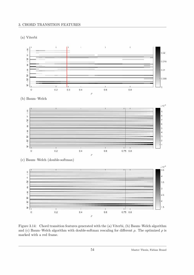
3. CHORD TRANSITION FEATURES
(a) Viterbi
(b) Baum–Welch
(c) Baum–Welch (double-softmax)
Figure 3.14: Chord transition features generated with the (a) Viterbi, (b) Baum–Welch algorithmand (c) Baum–Welch algorithm with double-softmax rescaling for different ρ. The optimized ρ ismarked with a red frame.
54 Master Thesis, Fabian Brand

3.4 PIECE-LEVEL CHORD TRANSITION FEATURES
less information. By these considerations, the optimal ρ must be somewhere in between. For
the Bach choral, the value ρ = 0.75—as optimized on the Beatles dataset—seems to be a good
compromise. We also see, that the vector is not very sensitive to small changes of ρ. Thus, small
deviations should still yield similar results.
If we perform double-softmax rescaling before the feature aggregation, we obtain a different
behavior (see Figure 3.14c). Around standard ρ, we clearly see the relevant transitions. When
we decrease ρ, the vector becomes sparser and “lattice” transitions become dominant. We have
to keep in mind that the softmax parameters were visually optimized on a chord transition
estimation result with ρ = 0.75. Therefore, we cannot expect the algorithm to work for other
values of ρ. Note that those arguments are purely qualitative and based on only one example.
We perform a more systematic examination in Chapter 5.
55 Master Thesis, Fabian Brand


4. BACKGROUND: STYLE CLASSIFICATION
Chapter 4
Background: Style Classification
In this chapter, we introduce the problem of musical style classification. Knowledge of a musical
style can be important in tasks like music retrieval or to categorize a music library. To classify
the style of a recording, we need a good classifier as well as suitable features. We covered our
proposed feature generation algorithms in the previous chapter. In this chapter, we introduce
the remaining components of the problem. At first, we present the musical scenario of our
experiments. We describe the dataset and provide some background information to further
specify the problem. Afterwards, we briefly cover basic machine learning techniques, needed for
the classification. In the last section, we give a small overview over previous work in this area.
4.1 Musical Scenario
To systematically evaluate style classification systems, we need a good dataset that contains
recordings of different styles. In [45], Weiß introduced the CrossEra dataset for this purpose. The
dataset comprises four different sub-styles of Western classical music from 1650 until the present.
The dataset splits into four classes: Baroque, Classical, Romantic, and Modern. Therefore
the pieces cover four important historical periods or “eras”. Each style is represented by 400
recordings. Of those 400 recordings, there are each 200 piano and 200 orchestra pieces. For
some experiments, we need the subsets CrossEra-Piano and CrossEra-Orchestra, which consist
of only piano and orchestra pieces, respectively. Table 4.1 shows the content of the CrossEra
database, grouped by style and composer. We see that the database is balanced with respect to
styles and instrumentation but not with respect to the composers. Unlike pop music, there are
many different versions of one composition or work in classical music. Especially the popular
works have been performed and recorded many times. Each recording differs from the others
in several ways, including tempo, possibly key, specific instruments and recording equipment.
The CrossEra database mainly contains recordings from the Naxos label. In CrossEra-Piano,
57 Master Thesis, Fabian Brand

4. BACKGROUND: STYLE CLASSIFICATION
Figure 4.1: Number of recordings in the CrossEraMirror database in relation to the recordingsin CrossEra
Weiß only selected recordings performed on a modern grand piano [45]. This excludes the
harpsichord, which was commonly used in the Baroque era. This measure prevents a classification
based on the instrumentation. We perform most of our experiments on the CrossEra set. In
the end we validate our results using unseen data. For this purpose, we use another dataset,
called CrossEraMirror. As the name indicates, it comprises different recordings of the same
works as CrossEra. With this dataset we can perform cross-version experiments. Not every
recording in CrossEra has an equivalent in CrossEraMirror interpreting the same work. The
content of CrossEraMirror is also listed in Table 4.1. To visualize the difference between the two
databases, Figure 4.1 shows a pie chart with the distribution of the different eras in the database.
Each quadrant represents one era in the CrossEra database. The percentage which is also in
CrossEraMirror is colored fully, the part which is only in CrossEra is colored transparently. We
see that CrossEraMirror is no longer balanced with respect to era, since Modern and Baroque
are underrepresented. The dataset is also not balanced with respect to instrumentation.
4.2 Basic Machine Learning Concepts
In this section, we give a brief introduction of concepts connected with machine learning and
classification experiments. This is a wide field so we limit ourselves to topics relevant for this thesis.
At first, we explain the basic notions of machine learning—also known as pattern recognition—
58 Master Thesis, Fabian Brand

4.2 BASIC MACHINE LEARNING CONCEPTS
Style Composer Number of RecordingsCrossEra CrossEraMirror
Baroque 400 249Albinoni, Tomaso 23 3Bach, Johann Sebastian 121 121Corelli, Arcangelo 15 14Couperin, Francois 36 36Giustini, Lodovico 8 0Handel, George Frederic 38 16Lully, Jean-Baptiste 15 1Platti, Giovanni Benedetto 41 0Purcell, Henry 10 4Rameau, Jean-Phillipe 60 41Vivaldi, Antonio 33 13
Classical 400 270Bach, Johann Christian 30 11Boccherini, Luigi Rodolfo 23 23Cimarosa, Domenico 32 1Clementi, Muzio 33 31Dussek, Jan Ladislav 35 0Haydn, Johann Michael 11 0Haydn, Joseph 100 95Mozart, Wolfgang Amadeus 114 109Pleyel, Ignace Joseph 10 0Salieri, Antonio 12 0
Romantic 400 333Berlioz, Hector 8 8Borodin, Alexander 9 9Brahms, Johannes 37 37Bruckner, Anton 12 12Chopin, Frederic 29 29Dvorak, Antonin 12 12Faure, Gabriel 15 13Grieg, Edvard 40 40Liszt, Franz 34 25Mendelssohn-Bartholdy, Felix 48 25Mussorgsky, Modest 12 0Rimsky-Korsakov, Nicolai 7 4Saint-Saens, Camille 16 8Schumann, Clara 13 0Schumann, Robert 43 43Smetana, Bedrich 6 6Tchaikovsky, Peter Iljitsch 30 19Verdi, Giuseppe 20 20Wagner, Richard 9 9
Modern 400 216Antheil, George 8 0Bartok, Bela 29 20Berg, Alban 11 10Boulez, Pierre 11 0Britten, Benjamin 9 9Hindemith, Paul 38 28Ives, Charles Edward 6 0Messiaen, Olivier 42 0Milhaud, Darius 22 0Prokofiew, Sergej 37 12Schoenberg, Arnold 30 18Shostakovich, Dmitri 82 82Stravinsky, Igor 28 23Varese, Edgar 14 0Webern, Anton 17 5Weill, Kurt 16 0
Table 4.1: Content of the CrossEra and CrossEraMirror database grouped by style and composer.
59 Master Thesis, Fabian Brand

4. BACKGROUND: STYLE CLASSIFICATION
before we move on to the concept of cross validation, explain dimensionality reduction, and
describe the Gaussian classifier.
4.2.1 Basic Notions
Machine learning systems generate models which are able to predict the outcome of experiments [4].
The key aspect is that these models are not generated by a human but by a machine. The
machine is able to classify data using knowledge it gained from previous data. We use this
concept for our classification experiments by training a model for style classification based on
chord transition features. Each machine learning experiment consists of a training phase and a
test phase. In the training phase we train the model using one part of the available data. In the
test phase we classify the remaining data based on the trained model.
We distinguish supervised and unsupervised training methods. In supervised training, the system
knows the ground truth labels of the training data. Unsupervised training only uses unlabeled
data. A good example for unsupervised training is the Baum–Welch algorithm for HMM training,
since the true internal states of the HMM are not needed. Learning the Gaussian emissions from
labeled data as performed in Section 2.3 fall in the category of supervised methods [40].
Our system consists of three steps. The feature extraction stage transforms the raw data into
a new format which is suitable for the classification task. This part is covered in Chapter 3.
Dimensionality reduction reduces the number of elements of the features vector by finding
appropriate combinations of the feature components that have a high discriminative power. This
way we can discard irrelevant information. Finally, we use a classifier to compute the estimated
labels from the reduced features. The dimensionality reduction and the classifier require a
training phase.
For the classification to work, the features need to have a property called separability. The
features belonging to one class should be close to each other (low intra-class distance) and the
features of different classes should be far from each other (high inter-class distance) [15].
4.2.2 Cross Validation
Any experiment on machine learning systems consists of a training phase and a test phase. In
the training phase, we use data to train a model until it yields an optimal outcome. Now, the
system performs well on the training data, but there is not guarantee, that it performs well on
previously unseen data. The model might be too specific to generalize well. This problem is
known as overfitting a system and describes the loss of generality of the learned patterns [7].
Therefore, it is very important to evaluate the system only on data that was not used for training.
This way we are close to a real world scenario where we do not know the labels of the test data.
60 Master Thesis, Fabian Brand

4.2 BASIC MACHINE LEARNING CONCEPTS
Figure 4.2: Example of how a database can be split three times into test an training set in orderto perform a 3-fold cross validation.
It is common practice to split the database in two sets, the training set and the test set. Each
set is only used for training and testing, respectively. The results reported after the experiment
come only from the test set. To still use the entire dataset for evaluation a so-called cross
validation [38] is used. We split the whole dataset in n so-called folds and perform n experiments.
In each experiment we use one fold as test set and the remaining folds for training. In this case,
we talk of an n-fold cross validation. That way we can evaluate the classification system on all
elements of the set. Figure 4.2 shows an example of how a database can be split for a 3-fold
cross validation.
There are different constraints on how to perform the split. A very common one is stratification [28].
We call a set stratified if it contains an equal number of samples of each class. It makes sense
to stratify both the test and the training set. This can be achieved by successively assigning
randomly chosen samples from one class to each fold. Sometimes the structure of the dataset
does not allow perfect stratification. In this case we can either randomly delete or duplicate
samples within the set until the set is stratified.
In some datasets, there exist groups of samples that belong to the same class but have other
similarities. For example two recordings from the same album1 were probably recorded with the
same equipment and by the same people, with the same instruments. The characteristics of each
instrument, musician and equipment can contribute to the features. A certain recording engineer
for example could tend to suppress the high frequencies slightly stronger than their colleagues,
which has an impact on the features. A classifier might now use that information to determine
that two recordings come from the same album, thus inferring that they have the same style.
While this decision is probably correct, the classifier bases this decision on properties which are
not related to the musical style. The classifier would not work as well on other recordings of the
1In the context of classical music, the term “album” refers to a group of recordings which were recordedtogether, i.e. in the same recording session or live recordings of the same concert.
61 Master Thesis, Fabian Brand

4. BACKGROUND: STYLE CLASSIFICATION
same style processed by a different recording engineer. In the MIR society, this phenomenon is
known as the “album effect“ [12,47]. The album effect is one type of overfitting.
To avoid the album effect, we have to make sure that the whole album is either in the training
or the test set. That way we increase the probability of overfitting to an album. But, since we
excluded all samples which profit from the overitted classifier from the test set, the classifier
cannot use recording artifacts for the classification. We call this procedure an “album filter”.
Using such filters typically makes the results worse. But in this case, we benefit from a better
approximation to a real world scenario. Since the album annotations are incomplete in our
dataset, we instead introduce an even stronger restriction: the composer filter. Here, we make sure
that works from each composer only appear in either the training or the test set. The composer
filter includes an album filter, since each album in the database only contains compositions from
one composer. By this measure we also avoid influences of overfitting on a certain composer
style.
4.2.3 Dimensionality Reduction
Dimensionality reduction is used to further compress the features. A high dimensional feature
vector has several disadvantages, which are summarized as the curse of dimensionality [40, 42].
In general, we can say, that a system with high dimensional features is more prone to overfitting
and generalizes worse. However, low-dimensional features may carry less information. Thus the
parameters and strategy of the dimensionality reduction play a crucial role for the overall result.
We explain two basic algorithms: the principal component analysis (PCA) and linear discriminant
analysis (LDA). PCA is an unsupervised algorithm while LDA is supervised but, therefore, also
prone to overfitting.
4.2.3.1 Principal Component Analysis
This chapter is a brief summary of [40, Chapter 6.3], which gives a much more detailed introduction.
Principal component analysis, also known as Karhunen–Loeve transform serves two purposes.
First, the transform performs a linear operation on the feature vectors, such that all elements
become uncorrelated. The basis vectors of the new feature space are the principal components of
the training set, giving this method its name. The transform does not change the dimensionality.
However, now that the elements of the feature vector are decorrelated, we can easily compute the
variance of each element and discard the elements with the lowest variance, since they probably
have the smallest influence on the separability of the classes.
62 Master Thesis, Fabian Brand
4.2 BASIC MACHINE LEARNING CONCEPTS
The principal components are the eigenvectors of the correlation matrix Rf , which can be
estimated on a training set of P feature vectors fp, p ∈ [1 : P ]:
Rf =1
P
P∑p=1
fpfᵀp . (4.1)
We can now compute the eigenvectors ai in descending order with respect to the corresponding
eigenvalues λi. We summarize the eigenvectors in the transform matrix APCA. We can write the
transformed feature vector f as:
f = AᵀPCAf (4.2)
with the correlation matrix
Rf = AᵀPCARfAPCA = Λ. (4.3)
Here Λ denotes the eigenvalue matrix, a diagonal matrix with the eigenvalues as elements in
descending order along the main diagonal. We see from this equality that the eigenvalues of
Rf are equal to the variances of the feature elements in the new vector space. To reduce the
dimensionality of the feature space from P to Q ≤ P , we can take the first Q elements of the
transformed feature vector. We therefore define APCA ∈ RP×Q as the matrix containing the
eigenvectors corresponding to the k highest eigenvalues.
However, since the PCA does not take the class labels into account, the dimensionality reduction
might delete important information. It is possible that two classes are only separable in the
dimensions with low variance. In Figure 4.3 we show an example of PCA leading to a loss of
separability. We see that the two classes are linearly separable in the two dimensional plane.
Performing a PCA we obtain two principal components f1 and f2. When we project the set on
f1 both classes overlap. The set is not separable anymore. This example shows, that we must
use PCA with caution in order to not destroy important information.
4.2.3.2 Linear Discriminant Analysis
In contrast to principal component analysis, linear discriminant analysis is a supervised procedure.
Here, we jointly maximize the inter-class variance and minimize the intra-class variance. In the
new feature space the classes are compact and have a high distance from each other. That way
we keep maximal separability.
Again, we search for a matrix ALDA such that
f = AᵀLDAf (4.4)
63 Master Thesis, Fabian Brand

4. BACKGROUND: STYLE CLASSIFICATION
(a) (b)
Figure 4.3: This figure shows a dataset in two dimensions, which is processed with PCA (a).The principal components are drawn as a second set of axes. The length of the axes indicates thevariance of the dataset along this axis. Sub-figure (b) shows the distribution of the data pointswith respect to f1.
has the desired properties. Using Fisher’s criterion [11] as described in [40], the basis of this
vector space are the eigenvalues of S−1w Sb, with the intra-class scatter matrix Sw ∈ RP×P and
the inter-class scatter matrix Sb ∈ RP×P , with P as the size of the feature vectors. It can be
shown that for a C-class problem it is sufficient to choose the vectors corresponding to the C − 1
highest eigenvalues, since all other components would be linearly dependent to the first C − 1
components. In [40, Section 5.8], Theodoridis explains LDA in more detail.
Figure 4.4 shows the same dataset as in the previous section. This time we process the data
with LDA. The set is still separable in the two dimensional space. We draw the projection axes
LDA computed. We see that after the projection, most elements of class 1 are on the negative
range of the f axis whereas most class 2 elements are on the positive range. The classes are still
separable after we projected the data on f1. The histogram for the reduced data confirms this,
as we see that the classes do not overlap.
In [40] Theodoridis states that the LDA does not perform well on very high-dimensional data.
Particularly if the dimensionality exceeds the number of training samples per class, Sw is not
invertible anymore. Theodoridis suggests to combine PCA and LDA. In this approach, we first
reduce the dimensionality with PCA. Afterwards, we train LDA on the reduced vectors and
64 Master Thesis, Fabian Brand
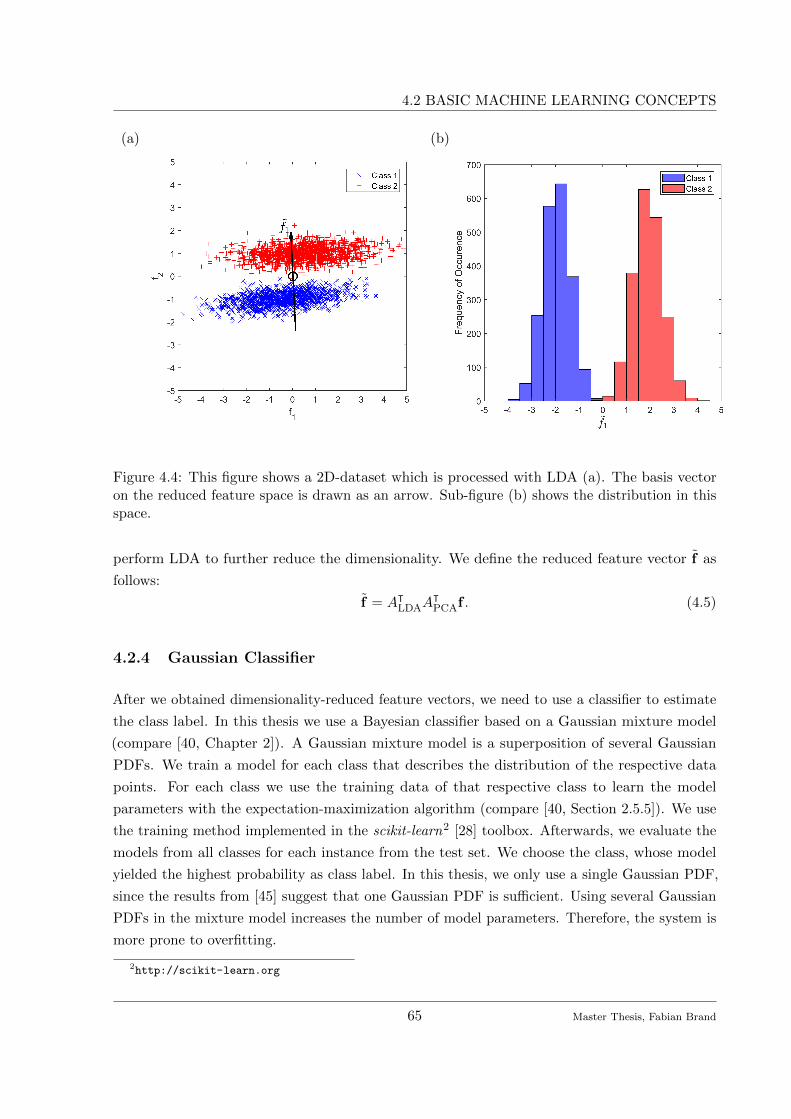
4.2 BASIC MACHINE LEARNING CONCEPTS
(a) (b)
Figure 4.4: This figure shows a 2D-dataset which is processed with LDA (a). The basis vectoron the reduced feature space is drawn as an arrow. Sub-figure (b) shows the distribution in thisspace.
perform LDA to further reduce the dimensionality. We define the reduced feature vector f as
follows:
f = AᵀLDAA
ᵀPCAf . (4.5)
4.2.4 Gaussian Classifier
After we obtained dimensionality-reduced feature vectors, we need to use a classifier to estimate
the class label. In this thesis we use a Bayesian classifier based on a Gaussian mixture model
(compare [40, Chapter 2]). A Gaussian mixture model is a superposition of several Gaussian
PDFs. We train a model for each class that describes the distribution of the respective data
points. For each class we use the training data of that respective class to learn the model
parameters with the expectation-maximization algorithm (compare [40, Section 2.5.5]). We use
the training method implemented in the scikit-learn2 [28] toolbox. Afterwards, we evaluate the
models from all classes for each instance from the test set. We choose the class, whose model
yielded the highest probability as class label. In this thesis, we only use a single Gaussian PDF,
since the results from [45] suggest that one Gaussian PDF is sufficient. Using several Gaussian
PDFs in the mixture model increases the number of model parameters. Therefore, the system is
more prone to overfitting.
2http://scikit-learn.org
65 Master Thesis, Fabian Brand
4. BACKGROUND: STYLE CLASSIFICATION
4.3 Related Work
This section provides an overview over related work in style classification. A musical style can
roughly defined by certain characteristics regarding instrumentation, melodic and harmonic
content, dynamics and timbre [18]. Assigning a piece to a style category can be ambiguous since
styles are not always well-defined, can possible overlap, and can be further divided [13]. Therefore
problem of style classification is an equally widespread problem consisting of many sub-problems.
We can distinguish between different genres, such as Jazz, Popular and Classical [29,30] or Chinese
folk music and Western popular music [35]. Some genres can be split in different sub-styles,
which poses the problem of sub-style classification. Here, we distinguish between sub-styles
belonging to the same genre. One example is our problem of era classification within Western
classical music [45]. Another example is the recognition of Jazz sub-styles in [19]. We can go
one step further and classify different composer within a (sub-)style. In [45], Weiß performs
experiments to distinguish between several Western classical composers. In [19], Hedges et al.
classify different Jazz composers.
Not only the set of styles varies within the problem of style classification, also the available
information for the feature calculation may be different. We can distinguish between symbolic
features and audio features. Symbolic features are based on symbolic music representations,
like sheet music or MIDI (Musical Instrument Digital Interface) files. In such approaches we
can directly use the musical information. In [31], Ponce de Leon and Inesta propose a set of
MIDI-based features that combine melodic, harmonic and rhythmic features. Armentano et al.
use MIDI-based features which describe sequences of MIDI events [1]. Ogihara and Li propose
MIDI-based chord progression features [27], by combining several chords to n-grams.
On the other hand, audio features are always based on a recording. One approach is the use of
standard audio features, like for example spectral envelope, zero crossing, or spectral flatness
measure. A common choice is also the mel frequency cepstral coefficient, which is also useful in
the field of speech recognition [41]. In [45], Weiß evaluates many of these features on the problem
of sub-style classification of Western classical music. While the features perform well without any
cross validation filter, the performance drops considerably when Weiß applies the composer filter.
Another possibility is the use of tonal features. Tonal features are designed to contain musical
information, such as features describing melody [34] or the frequency of chord transitions [45].
We call this kind of features, which have an explicit meaning, high-level features [45]. In [30],
Perez-Sancho et al. interpret the feature generation process as transforming the audio data to a
symbolic representation. On the other hand, there are mid-level features. In [45], Weiß defines
mid-level features as feature that “relate to human-interpretable concepts but in a way that is
not obvious.” He shows that tonal mid-level perform well in the context of sub-style classification
of Wester classical music.
66 Master Thesis, Fabian Brand

4.3 RELATED WORK
In [45], Weiß proposes features that describe the occurrence of certain intervals and chord
types. Weiß uses chroma templates describing each interval and each triad. The feature type is
based on the similarities between each chroma vector and each template vector. The feature
vector comprises the average and the standard deviation of those similarity measures across
the recording. Weiß also proposes features which quantify tonal complexity, referring to the
distribution of pitch class energies [47]. The feature consist of various complexity measures
quantifying for example sparsity of the chroma vector (low complexity) or the consonance (low
complexity) of corresponding notes.
Additionally Weiß introduces high-level chord transition features [45]. The feature requires
estimated chord labels. Weiß uses the Chordino system to estimate the chords with a large
chord vocabulary. However, the feature aggregation algorithm only considers transitions between
major and minor chords. In the end, the chord transition features contain information about the
relative frequencies of the chord transitions.
In [45] Weiß showed, that tonal features work well in a style classification scenario. The template-
based features showed the best performance. However, also the chord transition features yielded
good results. Both feature types performed well also with composer filter. We can interpret our
mid-level chord transition features as a conceptual combination of high-level chord transition
features and the mid-level template based features. The features proposed in [45] constitute the
baseline for the experiments in the following chapter. For a fair comparison we apply the same
classification pipeline on these and on our features.
67 Master Thesis, Fabian Brand


5. STYLE CLASSIFICATION EXPERIMENTS
Chapter 5
Style Classification Experiments
In this thesis, we focus on sub-style classification within Western classical music. In particular
we work on the CrossEra dataset described in Section 4.1. In this chapter, we present the style
classification experiments. At first, we introduce the classification pipeline, using the elements we
describe in Section 4.2. We start with baseline experiments by evaluating some of the features
described in [45] using our classification pipeline. Next, we give a comparison of the Viterbi-based
and the Baum–Welch-based features and test combinations of chord transition features, template
features, and complexity features. In the next experiments, we examine the influence of the
self-transition probability in the HMM on the classification results and also the combination of
different features. Furthermore, we look at the rescaling of the local chord transition features
(compare Section 3.2.2), which improve the visual results greatly. We then demonstrate the
album effect and examine how well different features generalize over different composers and
instrumentation. The chapter is concluded by cross-version experiments to verify the previous
results using the CrossEraMirror database. In this chapter, we give a detailed description of the
experiments. In Appendix B.3, we give summarized results, which extend the results presented
in this chapter.
5.1 Classification Pipeline
In the following experiments, we consistently use a specific processing pipeline to obtain our
classification results. We summarize the pipeline in Figure 5.1. We give an explanation of all
steps in the following. First, we divide the data set into a training set and a test set. We perform
the split employing a composer filter as described in Section 4.2.2 and forcing stratification
by randomly removing elements. We use about two thirds of the dataset for training and one
third for testing. In the next step, we extract piece-level features from the recordings of both
69 Master Thesis, Fabian Brand

5. STYLE CLASSIFICATION EXPERIMENTS
Figure 5.1: Visualization of the classification pipeline.
sets. We have already introduced the algorithms in Chapter 3. For comparison we also use the
template-based features from [46] and the complexity features from [47].
For dimensionality reduction we use PCA (Section 4.2.3.1) followed by LDA (Section 4.2.3.2).
First, we learn the PCA parameters on the training set. We then perform PCA using those
parameters on both sets. We reduce the feature dimensions to Q = 200 if the dimensionality is
greater than 200 and keep it constant if the feature vector has less than or exactly 200 dimensions.
If we perform experiments on the subsets CrossEra-Piano or CrossEra-Orchestra, we set this
threshold to 100 to account for the smaller training set. We need to use a dimensionality reduction
before LDA to avoid overfitting LDA. We found that the result is not sensitive on the exact
choice of this parameter as long as we choose Q smaller than the number of training samples but
not too small such that we delete important information. Setting the parameter Q to half the
number of samples per class seems to be a reasonable choice. For small feature vectors, we do not
need the PCA but for reasons of consistency, we always use it. In this case, we only decorrelate
the elements of the feature vector. LDA is performed similarly. First, we learn the parameters on
the training set and afterwards perform LDA on both sets. Since we are dealing with a 4-class
problem, the resulting reduced feature vector has only three dimensions. As mentioned in Section
4.2.3.2, LDA can only produce C − 1 independent components for a C-class problem.
We use the reduced feature vectors of the training set to train a Gaussian classifier, which then
classifies the test set. We compare the resulting estimated class labels to the annotation. We use
the accuracy as quality measure, which is the ratio of correctly classified recordings. We perform
a 3-fold cross validation (compare Section 4.2.2) such that we classify (almost) every recording
70 Master Thesis, Fabian Brand

5.2 BASELINE EXPERIMENTS
once. We repeat the cross validation ten times (ten “runs”) and average the accuracy of the
cross-validations to obtain a result that depends less on the specific splits. We make sure that
the splits are exactly the same for every experiment we perform by setting a fixed seed for the
random generators in each experiment. We also repeatedly tested random splits which yielded
similar results as the fixed splits we use in this thesis. The resulting mean accuracy of the 10
runs is the main quality measure of the used setting. However, we consider two more measures,
the inter-fold deviation and the inter-run deviation [39,45]. The inter-run deviation indicates the
stability over different splits. We average the accuracy over all three folds in each run. That way
we obtain mean accuracies for all ten runs. Afterwards, we compute the standard deviation of
these accuracies. On the other hand, the inter-fold deviation indicates the stability over different
test and training data. We first compute the standard deviation of the accuracies over all three
folds in each run. We obtain ten different standard deviations, which we then average. We use
the public toolbox scikit-learn to implement the machine learning algorithms.
5.2 Baseline Experiments
The goal of this section is to establish a baseline by comparing our features to the features used
for classification in [45]. We do not compare our results to the published results in detail. Instead
we use the same features as input for our own classifier. That way, we can be sure that the
circumstances are the same, since we use a slightly different classifier.
In this experiment we compare the features used in [45] to the proposed chord transition features
using the a chord vocabulary consisting of the 24 different major and minor triads. We select
the template-based features (denoted as “Template”), a combination of template-based and
complexity features (denoted as “Complexity & Template”) and the high-level chord transition
features as baseline features. To compute our features we need to model an HMM (compare
Section 2.4). We model the state transition matrix A with the method we discuss in Section
3.3. We use the standard values for ρ—we set ρ = 0.3 for Viterbi-based features and ρ = 0.75
for Baum-Welch-based features—as self-transition probability. We perform the experiments on
the full dataset CrossEra-Full, as well as on the instrumentation subsets, CrossEra-Piano and
CrossEra-Orchestra.
We give the results in Table 5.1. In this table we can see several interesting results. We see
that the Viterbi-based features and the chord transition features from [45] perform similarly.
This is according to our expectations, since we designed the Viterbi-based features with similar
concepts. We see that the Template features from [45] and the Complexity & Template features
perform better than all chord transition-based features. The distance is particularly high on the
CrossEra-Piano set, where the difference is around 10%. This behavior is consistent with the
results obtained in [45, Table 8.5].
71 Master Thesis, Fabian Brand

5. STYLE CLASSIFICATION EXPERIMENTS
Features CrossEra-Full CrossEra-Piano CrossEra-Orchestra
Template 73.9% 74.0% 79.4%Complexity & Template 74.7% 73.5% 79.3%Chord Transitions (from [45]) 67.2% 58.0% 72.1%Chord Transitions (Viterbi) 68.7% 60.8% 74.3%Chord Transitions (Baum–Welch) 69.3% 63.6% 75.8%
Table 5.1: Results of the baseline experiments. Different features from [45] and this thesis arecompared. We perform the experiments on the full dataset CrossEra-Full as well as the subsetsCrossEra-Piano and CrossEra-Orchestra.
Taking a look at the Baum–Welch-based features we see that they perform better than all other
chord transition features. However, the distance to the Viterbi-based features is only 0.6% for
the full CrossEra dataset. For the subsets the distance is bigger with 2.8% for CrossEra-Piano
and 1.5% for CrossEra-Orchestra. We also see, that the performance on piano pieces is worse
than on orchestra pieces. The piano pieces contain only a single instrument and therefore, have
less variation in the timbre than the orchestra which contains many instruments. We find this
behavior throughout all features, which is consistent with the results in [45]. We perform more
experiments on the subsets in Section 5.8.
5.3 Influence of Different Chord Vocabularies
As a next step, we compare the results obtained with different chord vocabularies. We tested
the MajMin, Triads and Sevenths chord vocabularies. The MajMin vocabulary contains all 24
major and minor triads. We extend this vocabulary with 4 augmented and 12 diminished triads
to the Triads vocabulary, which contains 40 chords. The Sevenths vocabulary contains the 75
different seventh chords we introduce in Section 2.1.2. In Table 5.2 we give the obtained results.
As first quality indicator, we use the obtained classification accuracy. Additionally, we give the
inter-run deviation, which we use to get an idea of the magnitude of the difference.
We see that the Baum–Welch-based features and the Viterbi-based features perform similarly for
the MajMin vocabulary. We observe different behaviors for features generated with the Viterbi
and the Baum–Welch algorithm as soon as we change the chord vocabulary. The Viterbi-based
features do not improve with increasing size of the chord vocabulary while the Baum–Welch-based
features yield better results. Since we expect roughly 300 chord changes in an average recording
of 10 minutes length, it is not possible to fully exploit all dimensions of high-dimensional feature
vectors like the 464-dimensional feature vector of the Sevenths vocabulary. Instead many elements
of the feature vector remain zero. We find the actual information only in a small part of the
feature vector. The Baum–Welch algorithm on the other hand does not have this problem. Here,
the underlying chord recognition scheme does not decide on one chord per time frame. Instead
72 Master Thesis, Fabian Brand

5.3 INFLUENCE OF DIFFERENT CHORD VOCABULARIES
Viterbi Baum–WelchVocabulary Dim. Accuracy Inter-Run Dev. Accuracy Inter-Run Dev.
MajMin 46 68.4% 0.6% 69.1% 0.8%Triads 132 68.8% 0.4% 72.6% 0.6%Seventh 464 67.8% 0.5% 74.6% 1.1%
Intervals 360 63.9% 0.9% 73.9% 0.7%
Table 5.2: Style classification results with different chord vocabularies. “Dim” denotes theoriginal dimensionality of the feature vector as obtained from the feature aggregation algorithm.
we have the probabilities of all possible transitions. We are able to exploit ambiguities in the
chord recognition process and are able to fully use the dimensionality of the feature vector. This
leads to clearly improved results. The observed gain of 5.3 % between the MajMin and the
Sevenths vocabulary is larger than the inter-run deviations.
Additionally, we define the Intervals vocabulary. This vocabulary comprises all 66 harmonic
intervals that are distinguishable in the equal tempered scale respecting octave invariance and
enharmonic equivalence. Note that we are not able to distinguish for example a major third over
C and a minor sixth over E. Also, due to symmetry, we can only distinguish six tritone intervals.
For example, the tritones over C and F] are indistinguishable. This vocabulary has a special role
in our system since it does not describe the chord transitions directly. However, every chord is
comprised of several intervals. We can therefore interpret a transition between two chords as
a superposition of several interval transitions. This is true for arbitrary chords such that we
are able to implicitly describe a larger chord vocabulary. We now have a generalized feature
which models all possible chords, avoiding problems like different numbers of notes per chord and
HMMs with many states. Note that the HMM with the Intervals vocabulary has 66 states which
is between the size of the Triads and Sevenths vocabularies. In Section 3.3, we observe a similar
effect when we interpret a seventh chord as superposition of a major and a minor triad. We also
see that this only works for the Baum–Welch algorithm, since the Viterbi algorithm decides on
one of the possibilities. The same is true in this case. We therefore expect good performance
for the Baum–Welch-based features but worse performance for the Viterbi-based features. The
results shown in Table 5.2 confirm this hypothesis. The Baum–Welch-based features perform
better than the Triads features and similarly to the Sevenths features, but the Viterbi-based
features perform about 5% worse than any other chord vocabulary. The Intervals vocabulary
shows the highest difference between Viterbi-based and Baum–Welch-based features.
We now present a more detailed analysis of the classification results. We start by looking at the
confusion matrix of the classification experiment. Using the confusion matrix we can analyze the
behavior of a classifier on a class level. Each entry of the matrix describes how often elements of
one class are classified as the other class. The elements on the main diagonal are the so-called
73 Master Thesis, Fabian Brand

5. STYLE CLASSIFICATION EXPERIMENTS
per-class accuracies. Figure 5.2 shows the confusion matrix for three different features. The first
matrix shows the results of the Baum–Welch-based features on the Triads vocabulary. There are
several interesting points. We see that the class Modern has the highest accuracy. This is in line
with musicology, since the rise of 12-tone music in this era has a very different chord structure.
Among other differences, this distinguishes the Modern era clearly from the other eras. There are
only very few confusions to the classes Baroque and Classical. About 10% of the recordings are
misclassified as Romantic. This is an expected behavior since the two respective time periods are
“neighbors” and have an overlap. In the earlier eras, we see many confusions between the classes
Baroque, Classical and Romantic. Here, a confusion to the direct neighbor is not preferred, in
fact confusions between Romantic and Baroque are more frequent than between Romantic and
Classical. This is consistent with the results found in [45, Figure 7.6], which stated that some
aspects of the chord transitions are more similar between the classes Baroque and Romantic than
between Baroque and Classical. The class Romantic has the smallest accuracy, which constitutes
a different behavior than observed in [45] with complexity and template-based features.
For the second matrix, we use the combination of complexity and template features from [45].
Here, we see the expected behavior, confusions to the “historically closer” eras are more common.
However, there are now more confusions between Baroque and Classical.
5.4 Combination of Features Types
Since our Baum–Welch-based features are not able to clearly separate Romantic from Baroque
but perform better in separating Baroque from Classical than complexity and template features,
we now combine the two features. We show the result in the third matrix of Figure 5.2. We see
that the per-class accuracies of Baroque, Classical, and Modern are larger than for either of the
previous features. The accuracy of the class Romantic is larger than for the Baum–Welch-based
features but slightly smaller than for the complexity and template features. We obtain an overall
accuracy of 76.1% (compare Table 5.3), which is higher than the overall accuracies of each
individual feature type alone. This shows that the information contained in both feature types is
of different nature, such that each feature type benefits from the other.
We take this as a motivation to examine other combinations of feature types. Table 5.3 shows the
classification accuracies of different feature combinations. We combine chord transition features
with either template features, complexity features or a combination of both. As a reference, we
also give the accuracies of the individual features alone (denoted with “None” in the respective
other feature class). We see that complexity features alone perform worse than the template
features, which agrees with the findings in [45]. We also see that a combination with Viterbi-based
features is not always beneficial, similar to the findings in [45], where a combination of chord
transition features with chroma-based complexity and template-based features is tested as well.
74 Master Thesis, Fabian Brand

5.4 COMBINATION OF FEATURES TYPES
(a) Baum–Welch-based (b) Complexity & Template
(c) Complexity & Template & Baum–Welch-based
Figure 5.2: Confusion matrix of classification experiments with (a) Baum–Welch-based features,(b) complexity and template features (see [45]) and (c) a combination of both features.
75 Master Thesis, Fabian Brand

5. STYLE CLASSIFICATION EXPERIMENTS
Chroma-Based Features Chord Transition FeaturesNone Viterbi Baum–Welch
None - 68.8% 72.6%Template 73.9% 74.4% 76.0%Complexity 64.4% 73.4% 75.9%Complexity & Template 74.7% 74.0% 76.1%
Table 5.3: Classification accuracies of combinations of chord transition features and chroma-basedfeatures from [45].
We can also repeat the findings, that a combination of Viterbi-based features and template-based
features performs best, better than the combination of Viterbi-based, Complexity, and Template.
However, in [45] this difference was higher. The behavior of the Baum–Welch-based features
differs from this. All combinations are better than each individual feature type. We obtain
the best overall performance for these combinations. Interestingly all combinations also have
very similar result. The differences of 0.1% are deemed insignificant. Apparently the amount of
additional style information is the same for complexity and template features. This is remarkable,
since complexity features alone have worse performance than template-based features. One
possible interpretation is that complexity features are of different nature than the chord transition
features. Therefore, there may be fewer overlap of the contained information. On the other hand,
template-based features contain information about occurrence frequencies of different chord types.
This information is related to our chord transition features. We can argue that much of the new
information from the Baum–Welch-base features is redundant with the information contained in
the template features.
In this section, we showed that—different to Viteri-based features—Baum–Welch-based contribute
information to the tonal features from [45] and are able to further improve the classification
accuracy up to 76%.
5.5 Influence of the Self-Transition Probability
In Section 3.4 we show the feature vectors of a single recording as a function of the self-transition
probability ρ. We concluded that the standard ρ has a value where we assume a good quality.
Those conclusions are only of qualitative nature since we did not yet have the possibility to test
the features in a classification experiment. We now use the features derived with the Triads chord
vocabulary using different values of ρ to classify the style of the recordings.1 The experiment
serves two purposes. First, we want to test if, a good chord recognition performance also leads
1We have to keep in mind that we obtain standard ρ by optimizing on a dataset consisting of modern popmusic, which is different to Western classical music. Also the result depends on the annotations as described inSection 3.3.
76 Master Thesis, Fabian Brand

5.5 INFLUENCE OF THE SELF-TRANSITION PROBABILITY
Figure 5.3: Classification accuracies for features generated with different ρ. The error barsindicate the inter-run deviation.
to efficient features. Second, we want to show that the gain of the Baum–Welch-based features
compared to the Viterbi-based features is actually due to the algorithm and not due to the
different choices of ρ.
In Figure 5.3, we show the classification accuracies of the Viterbi-based and the Baum–Welch-
based features as a function of ρ. Similar curves for the other chord vocabularies can be found
in Appendix B.2. We observe two results: The Baum–Welch-based features are superior to the
Viterbi-based features for all values of ρ. In fact, even the worst value of ρ for the Baum–Welch
algorithm performs better than the best for the Viterbi algorithm.
However, the assumption that a good chord recognition result leads to as good classification is
obviously flawed. The Baum–Welch-based features achieve the maximal accuracy of 77.0% for
ρ = 0.3. This is 5% higher than for the standard ρ = 0.75. We see that we can gain a 2.3%
better performance than the combination of complexity and template features as proposed in [45].
However, we have to keep in mind, that we optimize this hyper-parameter on the CrossEra
database and this particular feature setting. We do not use a separate cross validation, therefore
the value of ρ is probably overfitted. We therefore continue to use ρ = 0.75 for the rest of the
thesis since it lies in a relatively stable region. We assume that this holds also for other chord
vocabularies. We also see that the inter-run deviation indicated by the error bars rises suddenly
for ρ ≤ 0.15. This indicates an unstable behavior of the features. We should therefore avoid
Baum–Welch-based features with small values of ρ. Also, for large values of ρ, the Baum–Welch
algorithm yields good features.
For the Viterbi algorithm, the optimal ρ is not far off the standard ρ = 0.3, therefore we continue
to use it. We observe a drop of almost 10% for large values of ρ compared to standard ρ.
77 Master Thesis, Fabian Brand

5. STYLE CLASSIFICATION EXPERIMENTS
ρ 0.1 ρstd 0.9 {0.1, ρstd} {ρstd, 0.9} {0.1, ρstd, 0.9} ρopt
Viterbi 69.9% 68.8% 62.1% 69.8% 67.5% 70.2% 70.0%Baum–Welch 71.8% 72.6% 71.8% 75.7% 73.4% 73.9% 77.0%
Table 5.4: Results for combinations of features with different ρ.
This is probably due to the increasing sparsity of the feature vectors which we demonstrate
in Figure 3.14. However, for ρ = 0, we still obtain an accuracy of 66.0%, which is quite high,
considering the feature vector contains almost only noise-like transitions. Since the Viterbi-
algorithm switches chords in each frame, those transitions which are not musically relevant
predominate. In Figure 3.14 we see that most of those transitions are transitions between chords
which have two notes in common. Interestingly, those transitions also seem to convey style
information. Since Baum–Welch-based features also contain many of such transitions, this could
be one reason for their good performance. To test this hypothesis, we delete all such transitions
from the Baum–Welch-based feature vectors. However, we still obtain an accuracy of 72.4% for
ρ = 0.75, which is only slightly worse than for the full feature vectors. We can therefore conclude
that the high performance of the Baum–Welch-based features is not due to those “confusion
transitions”.
Features created with different values of ρ may have different semantic meaning. For small values
of ρ, we measure the local behavior of chords, possibly taking non-chord notes into account. For
large values of ρ, we measure chord changes on a larger scale, which can hint towards key changes.
This information can possibly increase the performance of the classifier. We therefore combine
features obtained with different values of ρ. By doing so, we hope to capture more information in
the feature vector. On the other hand, we also increase the dimensionality of the feature vector,
which also yields problems. For a good comparison between Viterbi- and Baum–Welch-based
features we combine the features with the standard ρ and features with ρ = 0.1 and ρ = 0.9. We
test combinations of the set {0.1, ρstd, 0.9}, with ρstd = 0.3 for the Viterbi-based features and
ρstd = 0.75 for the Baum–Welch-based features. Table 5.4 shows the results. As a reference we
present results for all three individual values of ρ as well as for ρopt, the (overfitted) value for ρ
that yields the best classification accuracy.
For the Baum–Welch-based features, we see that the results of the combined features are always
higher than for the individual feature types. A combination of ρstd with ρ = 0.1 works best,
probably because ρstd = 0.75 is already pretty high. However, we do not reach the maximal
accuracy at ρopt = 0.3. For the Viterbi algorithm, a combination of all three values of ρ can
exceed the maximum accuracy, though only by 0.2% and not enough to justify the increased
effort. The other combinations do not lead to improved features. A reason for this may be that
ρstd is already close to ρopt.
78 Master Thesis, Fabian Brand

5.6 INFLUENCE OF RESCALING
Figure 5.4: Classification accuracies for different rescaling parameters η1, η2.
5.6 Influence of Rescaling
In Section 3.2, we show that a non-linear rescaling improves the visual perception of local chord
transitions features. For this purpose we propose a double-softmax rescaling of ξn (i, j) which is
able to enhance the “musically relevant” transitions, see Algorithm 3.2. In Section 3.4, we visually
show the effect rescaling has on the piece-level chord transition features. We see that we are
able to suppress transitions which probably were musically irrelevant. In this section, we test if
there is also a qualitative improvement of the classification results when we apply double-softmax
rescaling. For this purpose we generate features based on the Triads chord vocabulary using the
Baum–Welch algorithm. Before feature aggregation we apply double-softmax rescaling on ξn (i, j).
We perform a grid search over the softmax parameters η1 and η2 with η1 ∈ {0, 5, . . . , 100} and
η2 ∈ {0, 2000, . . . , 40000}. Here, η1/2 = 0 denotes the case that we do not perform the respective
softmax. A parameter set of (η1, η2) = (0, 0) is therefore the case without any rescaling.
Figure 5.4 shows the result as an intensity plot. We see that the maximum accuracy lies at
(η1, η2) = (0, 0) with 72.6%. Even though rescaling with (η1, η2) = (10, 10000) yields very good
visual results for the Bach choral, we see that such a rescaling performs worse in a classification
scenario with an accuracy of only 60.1%. We see that the performance gets better again for large
η2. For (η1, η2) = (15, 40000) we obtain an accuracy of 69.0%. Even though the performance
is still worse than without any rescaling, the existence of good accuracies for high η2 is still
interesting, so we further investigate this setting. For this purpose, we look at the confusion
matrices for (η1, η2) = (15, 40000) and compare it with the confusion matrix for (η1, η2) = (0, 0)
79 Master Thesis, Fabian Brand

5. STYLE CLASSIFICATION EXPERIMENTS
(a) (b)
Figure 5.5: Confusion matrices for (η1, η2) equal to (a) (0, 0) and (b) (15, 40000).
in Figure 5.5. We see that all per-class accuracies are smaller for rescaling but the general
behavior of era confusions does not change. We therefore conclude that the semantic information
carried in the features is similar.
There are two possible reasons for the bad performance of the features vectors obtained with
rescaling: It is possible that rescaling deletes important information. The other possibility is that
the rescaling algorithm reacts too sensitive on the content and is therefore not able to perform
equally for all recordings, such that the feature vectors differ too much, also within one class.
5.7 Reduction to Major and Minor Chord Types
When we compare the way of obtaining chord transition features in [45] with our method, we
see several differences. In [45] Weiß performs chord estimation with a large chord vocabulary,
before reducing the resulting chord labels to major and minor chord types. The idea behind this
procedure is to only consider musically meaningful transitions, since forcing an augmented chord
into either a major or minor triad is musically incorrect. To this end, we map only chords which
were based on a major triad (also major seventh chords for example) to a major chord. We treat
chords based on a minor triad accordingly. Chords which are neither based on a major nor a
minor triads are ignored. In the following we define a chord as “based on a major or minor triad”
if the three lowest notes form the respective triad.
80 Master Thesis, Fabian Brand

5.7 REDUCTION TO MAJOR AND MINOR CHORD TYPES
Mapping Flexible Strict NoneOrignal Vocabulary Triads Sevenths Triads Sevenths MajMin Triads Sevenths
Viterbi 66.5% 62.4% 66.1% 61.3% 68.4% 68.8% 67.8%Baum–Welch 70.5% 70.8% 67.9% 71.3% 69.1% 72.6% 74.6%
Table 5.5: Results of experiments with reduced chord vocabularies.
In our experiments with the MajMin vocabulary we only allow major or minor triads. Thus, we
force every chord into the scheme of major and minor triads. We now want to reduce the Triads
and Sevenths vocabulary to major and minor triads, in order to make the results comparable to
the work in [45]. We can employ two strategies here. First, we map every chord to a major or
minor triad according to the lowest third interval. This should resemble the strategy when we use
the MajMin vocabulary. We call this strategy a “flexible mapping”. The other strategy is taken
from [45], where we tale only chords which are based on a major or minor triad into account.
We discard all other chords and the respective transitions. We call this a “strict mapping”. In
Table 5.5 we show the results of experiments with different mappings. As a reference we give the
accuracy obtained when we use the MajMin vocabulary already in the chord estimation stage, as
well as the accuracies of the Triads and Sevenths chord vocabulary.
We see that the result with reduced vocabularies is always worse than any non-reduced vocabulary
for the Viterbi algorithm. We observe that reduction from the Sevenths vocabulary is worse than
from the Triads vocabulary. Note that the non-reduced Sevenths vocabulary also performs slightly
worse than the Triads vocabulary. Furthermore, we see that the strict reduction performs worse
than the flexible reduction, but only by a small difference. One explanation of why the flexible
mapping performs worse than the MajMin vocabulary may be the following: For the flexible
reduction we perform a mapping which is similar to the mapping the Viterbi algorithm implicitly
performs when using the MajMin vocabulary. However, the Viterbi-algorithm optimizes the
chord sequence in context. Performing the mapping after the algorithm ignores this context and
may therefore lead to worse features. In general, we delete much information with the mapping.
Since each frame contains only information about one transition, we delete the information
contained in this frame completely for strict mapping.
Again the Baum–Welch-based features behave differently. Here, we see that the results improve
by at least 1% compared to the MajMin vocabulary. An exception is the strict mapping of
the Triads vocabulary. This may be due to the loss of information again. However, even for
strict mapping we still conserve information from the frame, which describes major and minor
chord types. For the Baum–Welch-based features a reduction from the Sevenths vocabulary
performs better than from the Triads vocabulary. We need to keep in mind that features
with a reduced chord vocabulary always show a worse performance than the features using the
81 Master Thesis, Fabian Brand

5. STYLE CLASSIFICATION EXPERIMENTS
Setting No Filter Composer Filter Piano → Orchestra Orchestra → Piano
Viterbi 66.4% 64.3% 67.1% 58.4%Baum-Welch 77.4% 72.6% 69.4% 65.9%
Table 5.6: Style classification accuracies and inter-fold deviations (Dev.) for various featureswhen different filters were applied.
respective non-reduced vocabulary. However, we show that we can improve the performance of
major-minor-based feature types by mapping from a larger vocabulary.
5.8 Influence of the Album Effect
One result from [45] is that standard audio features such as audio spectral envelope, spectral
flatness measure or mel frequency cepstral coefficients are not suitable for style classification,
since those features mainly capture timbral information. Weiß [45] found that the features
perform well without any constraints to the cross validation splits but failed with a composer
filter. The conclusion was, that the classifier overfits due to recording artifacts of an album
and uses these properties for classification. This effect is called “album effect”. Employing a
composer filter prevents that effect. Tonal features, on the other hand performed better with
album filter.
In the previous sections, we already showed that our features work well also with a composer
filter. In this section, we want to examine the effect of different cross validation strategies in
detail. To this end, we compare the results in four different settings. First, we use no filter, which
probably gives the best results since we can exploit recording artifacts and the personal style of
the composer. Both properties simplify the separation of classes in CrossEra, but were excluded in
the previous experiments on purpose. Second, we apply the composer filter as used in the previous
sections. In the end, we train the classifier on CrossEra-Piano and test on CrossEra-Orchestra
(“Piano → Orchestra”) and vice versa (“Orchestra → Piano”). Since the timbral content of both
instrumentation classes is different, those settings assure that we only use tonal information for
classification. We summarize both settings under the name “instrumentation filter”, but report
both experiments separately. We test Viterbi-based and Baum–Welch-based features and show
the results in Table 5.6.
As expected we see that the features perform better without filter than with composer filter. As
previously discussed, the reason here is overfitting on non-musical information. We see that the
drop of quality when we apply the composer filter is higher for Baum–Welch-based features than
for Viterbi-based features. We assume that this is due to a larger amount of timbral information
as a result from the soft-decision algorithm. For the instrumentation filter we look at the single
82 Master Thesis, Fabian Brand
5.8 INFLUENCE OF THE ALBUM EFFECT
results of both possible setups. We see that training on piano recordings and testing on orchestra
recordings yields better results than the reversed case. Weiß observes the same tendencies in [45].
Interestingly, for “Piano → Orchestra”, the Viterbi-based features perform better than without
filter, but the reversed case is roughly 10% worse. For the Baum–Welch-based features, both
results are worse than the results with composer filter, but there is only a difference of 3.5%
between both directions. This is a more stable behavior than the Viterbi-based features. We
see that the instrumentation filter results are on average about 5% below the composer filter
for Baum–Welch based features and less than 2% for Viterbi-based features. Those are better
results than Weiß [45] obtains with template features, where accuracy dropped by roughly 10%
compared to the composer filter.
We see that, even though the Viterbi-based features perform well under the instrumentation
filter in average, the individual results show an unstable behavior. The Baum–Welch algorithm
shows a different behavior. Here, the loss due to the instrumentation filter is higher, but the
features perform comparably in both directions.
We observe another interesting difference when we perform the experiment for different self-
transition probabilities ρ. In Figure 5.6, we show the accuracies of all four experiments as a
function of ρ for both Baum–Welch-based features and Viterbi-based features. We observe that
the difference between the curves for “no filter” and the composer filter is independent of the
chosen value of ρ for both algorithms. For the Baum–Welch-based features, the performance of
the instrumentation filter generally decreases with decreasing values of ρ. From the experiments
on the Bach choral in Section 3.3, we know that there are more transitions present for smaller
values of ρ, which points towards a larger amount of timbral information. This is one possible
explanation for this result, since we assume that a larger amount of timbral information leads to
worse generalization over different instrumentations. Interestingly, the curve for the composer
filter does not decrease accordingly. We therefore conclude that the reason behind the loss
of accuracy with composer filter is at least partially different to the reason behind the loss
with instrumentation filter. Additionally, this plot justifies the choice of ρ = 0.75 as standard
parameter for Baum–Welch-based features. The value of ρ which yields the highest result with
the composer filter (ρ = 0.3) shows worse results with instrumentation filter. We therefore
consider this feature type less robust against changes in instrumentation.
If we look at the Viterbi-based features, we see that the features behave unstable in an instru-
mentation filter scenario, in a sense of a large difference between the two cases, for all values of ρ.
However, we see that—different to the Baum–Welch-based features—the loss due to the instru-
mentation filter does not depend on ρ. Since we connect this loss with the presence of timbral
information, we conclude that the timbral content of Viterbi-based features is independent of the
chosen value of ρ. An exception are features obtained with low values of ρ, where the accuracy
83 Master Thesis, Fabian Brand

5. STYLE CLASSIFICATION EXPERIMENTS
(a) Baum–Welch-based features
(b) Viterbi-based features
Figure 5.6: Classification accuracy of (a) Baum–Welch-based features and (b) Viterbi-basedfeatures for different ρ and different filters.
84 Master Thesis, Fabian Brand

5.9 CROSS-VERSION EXPERIMENTS
Era Selected Composers
Baroque J.S. Bach, CorelliClassical Boccherini, Haydn, ClementiRomantic Brahms, Grieg, R. Schumann, BrahmsModern Bartok, Berg, Schoenberg, Shostakovich
Table 5.7: Composers we chose for the test set of the cross-version experiment. The recordingsof all remaining composers comprise the training set.
drops suddenly for the instrumentation filter. We showed in Section 3.3, that also Viterbi-based
features capture much timbral content for small ρ, which is in line with our hypothesis.
In general, we can say that Baum–Welch-based features are influenced more by a composer
or instrumentation filter. Nevertheless, Baum–Welch-based features still perform better than
Viterbi-based features. Additionally, we observe an unstable behavior for the Viterbi-based
features with instrumentation filter, since Viterbi-based features do not generalize well from
orchestra data to piano data. We also found that the influence of the composer filter is weaker
for chord transition features in general than for other tonal features proposed in [45].
5.9 Cross-Version Experiments
As a final experiment, we want to verify our classifier with cross-version experiments. For
this purpose, we use the CrossEraMirror dataset. As described in Section 4.1, the database
contains different recordings of a subset of the works in the CrossEra dataset. We did not use
CrossEraMirror in previous experiment. We do not perform extensive research on CrossEraMirror
to avoid presenting overfitted results. We use the CrossEraMirror database in two scenarios.
First, we perform classification on one single split in training and test set, which was manually
created to resemble the previous experiments as closely as possible. We use a composer filter
and select composers for the test set, such that the test set contains roughly one third of the
samples (compare Table 5.7). Afterwards, we discard all recordings that are not part of the
CrossEraMirror database from the test set. We use the recordings from all the remaining
composers for the training set. We stratify both sets using random deletion. Afterwards, we
train a classifier on the training set by using recordings from CrossEra and test the classifier on
recordings from both databases separately. That way we test, how well the features generalize
over different versions. In this experiment, we expect that the result we obtain when we test
on CrossEra data is better since recordings in CrossEra are from the same label as the training
data. We test Viterbi-based and Baum–Welch-based features with all chord vocabularies. We
give the results in Table 5.8. When evaluating this table we need to keep in mind, that we are
dealing with only one classification experiment without cross validation.
85 Master Thesis, Fabian Brand

5. STYLE CLASSIFICATION EXPERIMENTS
Viterbi Baum-WelchCrossEra CrossEraMirror ∆ CrossEra CrossEraMirror ∆
MajMin 71.2% 72.7% -1.5% 70.6% 69.0% 1.5%Triads 67.9% 68.5% -0.6% 72.7% 70.6% 2.1%Seventh 67.1% 65.2% 1.9% 75.0% 70.8% 4.2%
Intervals 61.3% 61.2% 0.2% 71.3% 69.8% 1.5%
Table 5.8: Results of the first experiment on CrossEraMirror. We use one manually createdsplit. We always train the model on CrossEra data and test on both datasets.
Surprisingly, the Viterbi-algorithm yields sometimes better results on CrossEraMirror than on
CrossEra. Since the deviations are comparatively small and go in both directions, it is possible
that the deviation is within the normal inter-fold deviation. In general, we see that Viterbi-based
features generalize well over different versions. When we average over all types of Viterbi-based
features, there is no difference between both databases.
The Baum–Welch-based features generalize worse over different versions. If we use the CrossEraMir-
ror database for testing, we see that the results are consistently worse than for CrossEra. We
observe a trend that the difference increases with larger chord vocabularies. In contrast, the
Intervals vocabulary shows a lower deviation again.
Since both databases differ mainly in timbral content—for example, CrossEraMirror contains
recordings of an harpsichord, which was excluded in CrossEra—this experiment supports the
hypothesis, that Baum–Welch-based features contain more timbral content. We have to keep in
mind that—except for the MajMin dataset—the Baum–Welch-based features still perform better
in terms of achieved accuracy.
For the second experiment, we use the CrossEraMirror database to simulate a “real” album filter.
Therefore, again, we train a model on data from CrossEra and then test it on CrossEraMirror. We
reduced both datasets to the works contained in CrossEraMirror. This way we can perform a cross
validation on both sets. We do not use any filter here, but since CrossEra and CrossEraMirror
contain no common album, the cross-version experiment contains an implicit album filter. We
show the results in Table 5.9. We see that most feature types have a similar behavior and loose
between 2% and 3% accuracy when we test them on CrossEraMirror. Reasons can include the
album effect or differences in instrumentation (grand piano in CrossEra and harpsichord in
CrossEraMirror). An exception are the Viterbi-based features on the MajMin vocabulary and
the Baum–Welch-based features on the Triads vocabulary, which perform better. We have no
explanation for these outliers. We cannot compare the results directly to the results from the
previous section, where we already showed experiments on CrossEra without any filter, since the
used datasets differ in various points, such as size and the distribution of the composers (also
compare Table 4.1). That way, we are dealing with a different task here.
86 Master Thesis, Fabian Brand

5.9 CROSS-VERSION EXPERIMENTS
Viterbi Baum-WelchCrossEra CrossEraMirror ∆ CrossEra CrossEraMirror ∆
MajMin 72.5% 72.0% 0.5% 74.6% 72.4% 2.2%Triads 73.7% 71.3% 2.4% 79.7% 78.2% 1.5%Seventh 73.1% 70.1% 3.0% 82.3% 79.6% 2.7%
Intervals 68.8% 66.3% 2.6% 80.6% 78.2% 2.4%
Table 5.9: Results of the second experiment performed on CrossEraMirror, which simulatesan album filter. We always train the model on CrossEra data but test on either CrossEra orCrossEraMirror.
We also perform the same experiment using the template features from [45]. We obtain an
accuracy of 76.0% when we test those features on CrossEraMirror as opposed to an accuracy of
82.8% on CrossEra. We see that chord transition features achieve better generalization than
template features. This is in line with the results in Section 5.8, where we examine generalization
over instrumentation.
To show the relationship between the features of both datasets, we use a scatter plot of the
reduced features after LDA in Figure 5.7. For this plot, we use Baum–Welch-based features on
the Triads vocabulary. We first look at the left column of plots. Here, we see the features from
the CrossEra dataset. To visualize the 3D-data obtained from LDA, each plot shows a different
combination of coordinates. Note that the classes are usually better separable than suggested by
a single plot. One plot shows only two coordinates, but a classifier can use all three coordinates
for classification. For the plots, we fitted LDA on the entire CrossEra dataset. The classes are
color-coded. The plots confirm our conclusions drawn from the confusion matrices in Section 5.4.
The classes Baroque, Classical, and Romantic are distinct but have overlapping regions. Those
overlaps are present in all plots. We see that the Modern class is clearly separable from Baroque
and Classical by the first discriminant but still has a few overlaps with Romantic. This is also
consistent with the previous results and the findings in [45].
On the right column we see an extension of the previous plots. Here, we show the same features
from CrossEra but we show the distance between the musically corresponding instances from
CrossEraMirror as a line connecting both instances. For orientation purposes, we mark the
instance from CrossEra. We see that the distance between the features can get rather large.
However the lines rarely cross the boundaries between the classes. This indicates a stable
work-level behavior in classification experiments.
In Figure 5.8 we show the same plot for features based on the Sevenths chord vocabulary. Again,
we use Baum–Welch-based features. We only display the projection on a single plane for both
datasets in one plot. We see that the classes are better separable than for the Triads dataset.
This is in line with the higher accuracies we obtain with the Sevenths vocabulary. However, we
87 Master Thesis, Fabian Brand

5. STYLE CLASSIFICATION EXPERIMENTS
(a) CrossEra (b) CrossEra—CrossEraMirror
(c) (d)
(e) (f)
Figure 5.7: Scatter plot of all instances from the CrossEra database. In the left column, eachpoint corresponds to one recording in the CrossEra database. In the right column, each lineconnects an instance vector from CrossEra with the musically corresponding instance fromCrossEraMirror. Each row shows the projection of the 3D-data on a different coordinate plane.We use features computed with the Baum–Welch algorithm and the Triads chord vocabulary.
88 Master Thesis, Fabian Brand

5.9 CROSS-VERSION EXPERIMENTS
Figure 5.8: Scatter plot showing the features of CrossEra connected with the features ofCrossEraMirror. We compute the features with the Baum–Welch algorithm and the Seventhschord vocabulary.
89 Master Thesis, Fabian Brand

5. STYLE CLASSIFICATION EXPERIMENTS
see several lines crossing the class boundaries. Most prominently, we see many features “moving”
from Modern to Romantic and from Romantic to Classical. That visualizes the difference between
the results of both datasets, which is also in line with the loss of accuracy we observe in Table 5.8
for the Sevenths vocabulary. We see that this kind of plot is suitable for showing the difference
between the two datasets.
In this section, we showed that chord transition features generally perform well in cross-version
experiments. We found differences between Baum–Welch-based features and Viterbi-based
features. The high-level Viterbi-based features generalize better over different versions. We
assume, this is due to only few timbral information. The results we presented here are in line
with the results from the previous sections.
90 Master Thesis, Fabian Brand

6. CONCLUSIONS
Chapter 6
Conclusions
In this thesis, we introduced a novel kind of mid-level chord transition features. Chord transition
features are useful for describing the harmonic progression of music recordings and contain
information about the frequency of different kinds of chord transitions. Chord transition features
described in previous work are high-level features, which directly describe properties of an
estimated chord sequence. This approach is based on chord recognition, which is usually done
with Hidden Markov Models and the Viterbi algorithm. In this thesis, we propose mid-level
features. We do not estimate a chord sequence from which we derive the transition features,
but rather compute transition probabilities based on the probabilistic Hidden Markov Model.
With this kind of features, we are able to take ambiguities in the chord estimation process into
account.
To compute local mid-level chord transition features, we made use of the Baum–Welch algorithm.
This algorithm was initially proposed to train a Hidden Markov Model. We derived state
transition probabilities from internal variables of the Baum–Welch algorithm. Extracting these
variables, we were able to perform a soft-decision chord transition estimation. For visualizing
the local mid-level chord transitions, we proposed a non-linear rescaling technique. In a chord
recognition scenario, we showed that this approach is able to display ambiguities in the recognition
process. We used these ambiguities to gain more musical knowledge than from a traditional
hard-decision chord recognition approach.
We also showed that we can use chord transitions to characterize a whole recording. We obtain
these piece-level chord transition features by averaging the chord-transition probabilities over the
entire sequence. We test these aggregated features in a style classification scenario, in which we
distinguish between the four musical periods Baroque, Classical, Romantic, and Modern within
Western classical music.
91 Master Thesis, Fabian Brand

6. CONCLUSIONS
In the classification experiments, the proposed Baum–Welch-based chord transition features
showed consistently better classification results than equivalent high-level Viterbi-based features.
Baum–Welch based features benefit from using a larger chord vocabulary, while the efficiency of
Viterbi-based features decreases with larger chord vocabularies. Even though chord transitions
are only one aspect to distinguish musical styles, our mid-level features show a performance
comparable to other state-of-the-art tonal features. We showed that a combination of the
mid-level chord transition features with those state-of-the-art tonal features performed better
than both individual feature types alone. We performed all experiments using a composer
filter, to prevent overfitting to non-musical properties known as the “album effect”. We also
tested the features without composer filter and found that the album effect has less impact
than on other mid-level tonal features. We also performed experiments in which we trained the
classifier on piano pieces and tested on orchestra pieces and vice versa. Here, we showed that
the Baum–Welch-based features are in general robust to different instrumentation. In contrast,
Viterbi-based features showed an unstable behavior.
There are several interesting topics concerning mid-level chord transition features, which could
be examined in future work. We found that the self-transition probability is an important
hyper-parameter of the Hidden Markov Model we used to generate our features. We observed
effects on the classification accuracies as well the features ability to generalize over different
instrumentations. In future work, one could further investigate the internal mechanisms leading
to this behavior and search for optimal values in a separate cross validation.
In this thesis we limited ourself to a template emission model. Cho and Bello [9] found that a
Gaussian emission model is generally more robust against changes in the self-transition probability.
We showed that a Gaussian model allows chord vocabularies containing chords with different
numbers of notes. Researching the applications of a Gaussian emission model to generate
mid-level chord transition features is therefore promising interesting results.
The usage of Hidden Markov Models gives us another interesting possibility for a different classifier.
Instead of creating features with the Baum–Welch algorithm, we could use this algorithm to train
one HMM for each class. Afterwards, we could classify a recording by evaluating the probability
of the respective chroma sequence within each model and choosing the class whose model yields
the highest probability. A similar approach is typically used for speech recognition tasks, such as
isolated word recognition [33]. However, first experiments did not show promising results for
style classification. In future work one could further investigate this method.
In this thesis we showed the high performance or our features in one specific scenario: classifying
recordings of Western classical music into four sub-styles. In future work we could examine
the features in other scenarios, such as in jazz or rock music. Also, changing the classification
objective, such as classifying different composers or looking for applications in work identification
is possible.
92 Master Thesis, Fabian Brand

6. CONCLUSIONS
In summary, this thesis shows that it is possible to combine the benefits of chord transition
features with the concept of mid-level, soft-decision features. The resulting features are robust
against the album effect, generalize well across instrumentations, and perform better than
comparable high-level chord transition features, based on hard-decision chord estimation.
93 Master Thesis, Fabian Brand


A. HIDDEN MARKOV MODELS
Appendix A
Hidden Markov Models
In this chapter, we derive the equations for the forward and backward algorithm and the
calculation of the local state transition probabilities ξn (i, j), which were introduced in Section 3.2.
We use the notations and definitions introduced there.
A.1 Forward Algorithm
First, we recall the definition of the forward variable vn (i) (Eq. 3.13):
vn (i) = P (o1o2 . . .on, sn=αi|Θ) (A.1)
For n = 1 we can write:
v1 (i) = P (o1, s1 =αi|Θ) = P (s1 =αi|Θ)P (o1|s1 =αi,Θ) = cibi(o1), (A.2)
using the chain rule. That way we arrive at the initialization step. To derive the iteration
step, we need to use the Markov property. It states, that the current state only depends on the
previous state. Let Oba with 1 ≤ a < b ≤ N denote the subsequence [oaoa+1 . . .ob]. We write:
vn (j) = P(On−1
1 on, sn=αj |Θ)
=
= P(On−1
1 , sn=αj |Θ)P(on|On−1
1 , sn=αj ,Θ) (A.3)
Since on only depends on sn and not directly on the previous observations (the observations are
not statistically independent but all information passes through sn, therefore all other conditions
are redundant). We can write
P(on|On−1
1 , sn=αj ,Θ)
= P (on|sn=αj ,Θ) = bj(on) (A.4)
95 Master Thesis, Fabian Brand

A. HIDDEN MARKOV MODELS
We can rewrite the other part of Eq. A.3 by reverse marginalization:
P(On−1
1 , sn=αj |Θ)
=
I∑i=1
P(On−1
1 , sn=αj , sn−1 =αi|Θ). (A.5)
We now see that
P(On−1
1 , sn=αj , sn−1 =αi|Θ)
= P(sn=αj |On−1
1 , sn−1 =αi,Θ)P(On−1
1 , sn−1 =αi|Θ)
=
= P (sn=αj |sn−1 =αi,Θ)P(On−1
1 , sn−1 =αi|Θ)
=
= aijvn−1 (i) .
(A.6)
In the second line we use the Markov property again to eliminate a condition. By combining
Eqs. A.3–A.6, we obtain the known iteration step formula.
A.2 Backward Algorithm
We now derive the equations for the backward algorithm. Here, we have the problem that
according to the definition
wn (i) = P (on+1on+2 . . .oN |sn=αi,Θ) (A.7)
the initial variable wN (i) is not defined. We therefore first derive the iteration step and then
show, that wN (i) = 1 ∀i yields the desired result. We start be rewriting the definition with
the shorthand notation Oba = [oaoa+1 . . .ob] with 1 ≤ a < b ≤ N and applying a reversed
marginalization:
wn (i) = P (on+1on+2 . . .oN |sn=αi,Θ)
= P(on+1O
Nn+2|sn=αi,Θ
)=
I∑j=1
P(on+1O
Nn+2, sn+1 =αj |sn=αi,Θ
).
(A.8)
We can further expand the summands by applying the chain rule:
P(on+1O
Nn+2, sn+1 =αj |sn=αi,Θ
)=
=P (sn+1 =αj |sn=αi,Θ)P(on+1O
Nn+2|sn+1 =αj , sn=αi,Θ
)=
=aij · P(on+1O
Nn+2|sn+1 =αj ,Θ
).
(A.9)
96 Master Thesis, Fabian Brand

A.3 LOCAL STATE TRANSITION PROBABILITIES
In the last step we use the definition of the transition probability and the fact that the future
output only depends on the previous state through sn+1, which follows from the Markov property.
We continue with
P(on+1O
Nn+2|sn+1 =αj ,Θ
)=
=P (on+1|sn+1 =αj ,Θ)P(ONn+2|on+1, sn+1 =αj ,Θ
)=
=P (on+1|sn+1 =αj ,Θ)P(ONn+2|sn+1 =αj ,Θ
)=
=bj(on+1)wn+1 (j)
(A.10)
Combining all above equations we arrive at the iteration step. We can explicitly compute
wN−1 (i):
wN−1 (i) = P (oN |sN−1 =αi,Θ) =
=I∑j=1
P (oN , sN =αj |sN−1 =αi,Θ) =
=I∑j=1
P (sN =αj |sN−1 =αi,Θ)P (oN |sN =αj , sN−1 =αi,Θ) =
=
I∑j=1
aijbj(oN ) · 1.
(A.11)
The calculation steps follow the same scheme as the previous derivation. We see that this
expression is equivalent to the iteration step, if we set wN (i) = 1 ∀i. Therefore we use this as
initial value for the iteration.
A.3 Local State Transition Probabilities
To prove Equation 3.15 we first rewrite the conditional probability of Eq. 3.12 using Bayes’
theorem:
ξn (i, j) = P (sn=αi, sn+1 =αj |O,Θ) =
=P (sn=αi, sn+1 =αj , O|Θ)
P (O|Θ)
(A.12)
97 Master Thesis, Fabian Brand

A. HIDDEN MARKOV MODELS
In the following we only consider the enumerator. Let Oba with 1 ≤ a < b ≤ N denote the
subsequence [oaoa+1 . . .ob].
P (sn=αi, sn+1 =αj , O|Θ) =
=P(sn=αi, sn+1 =αj , O
n1O
Nn+1|Θ
)=
=P (On1 , sn=αi, sn+1 =αj |Θ) · P(ONn+1|On1 , sn=αi, sn+1 =αj ,Θ
) (A.13)
Using the Markov property, we see that any observation at time n+ 1 or later only depends on
previous states and observations through the state sn+1. Of course they are not statistically
independent but all information passes through sn+1, therefore all other conditions are redundant.
With this consideration we write:
P(ONn+1|On1 , sn=αi, sn+1 =αj ,Θ
)=
=P(ONn+1|sn+1 =αj ,Θ
)=
=P(on+1O
Nn+2|sn+1 =αj ,Θ
)=
=P (on+1|sn+1 =αj ,Θ) · P(ONn+2|on+1, sn+1 =αj ,Θ
)=P (on+1|sn+1 =αj ,Θ) · P
(ONn+2|sn+1 =αj ,Θ
)(A.14)
In the last step we can eliminate one condition by similar considerations as above. Using the
definitions of the backward variable (Eq. 3.14) and emission probability (Eq. 2.16) we see:
P (on+1|sn+1 =αj ,Θ) · P(ONn+2|sn+1 =αj ,Θ
)=
=P (on+1|sn+1 =αj ,Θ) · P (on+2 . . .oN |sn+1 =αj ,Θ) =
=bj(on+1) · wn+1 (j)
(A.15)
We now further analyse P (On1 , sn=αi, sn+1 =αj |Θ) from Eq. A.13
P (On1 , sn=αi, sn+1 =αj |Θ) =
=P (On1 , sn=αi|Θ) · P (sn+1 =αj |On1 , sn=αi,Θ) =
=P (On1 , sn=αi|Θ) · P (sn+1 =αj |sn=αi,Θ)
(A.16)
Again one condition could be eliminated by the Markov property, this time by exploiting that a
state is connected to previous observations only via the previous state. The resulting expression
can be directly rewritten as
P (On1 , sn=αi|Θ) · P (sn+1=αj |sn=αi,Θ) = vn (i) · aij . (A.17)
Combining Eqs. A.12 – A.17 we arrive at the expression in Eq. 3.15.
98 Master Thesis, Fabian Brand

B. FURTHER RESULTS
Appendix B
Further Results
B.1 Influence of the Self-Transition Probability
on Chord Recognition
In this section, we show plots to demonstrate the chord recognition performance of the Viterbi
algorithm and the Baum–Welch algorithm for different values of ρ. In Figure B.1, we show the
results of the Viterbi algorithm and in Figure B.2, we show the soft-decision results obtained
with the Baum–Welch-algorithm. Here, we use a single softmax η = 10 on the state probabilities
to visualize the probabilities better. As in Figure 3.7 we choose the parameter ρ from the set
ρ ∈ {0.025, 0.02, 0.5}.
99 Master Thesis, Fabian Brand

B. FURTHER RESULTS
(a) ρ = 0.025
(b) ρ = 0.2
(c) ρ = 0.5
Figure B.1: Viterbi-based chord recognition of the Bach example for different values of ρ.
100 Master Thesis, Fabian Brand

B.1 INFLUENCE OF THE SELF-TRANSITION PROBABILITY ON CHORDRECOGNITION
(a) ρ = 0.025
(b) ρ = 0.2
(c) ρ = 0.5
Figure B.2: Baum–Welch-based chord recognition of the Bach example for different values of ρ.
101 Master Thesis, Fabian Brand

B. FURTHER RESULTS
B.2 Influence of the Self-Transition Probability
on Style Classification
In this section, we show several plots which show the influence ρ has on the classification accuracy.
Figure B.3 shows the results for the MajMin and Triads vocabularies, and Figure B.4 shows the
results for the Sevenths and Intervals vocabularies. The plots support the results obtained in
Section 5.6.
(a) MajMin
(b) Triads
Figure B.3: Classification accuracy as a function of ρ for the MajMin and Triads vocabularies.
102 Master Thesis, Fabian Brand

B.2 INFLUENCE OF THE SELF-TRANSITION PROBABILITY ON STYLECLASSIFICATION
(a) Sevenths
(b) Intervals
Figure B.4: Classification accuracy as a function of ρ for the Sevenths and Intervals vocabularies.
103 Master Thesis, Fabian Brand

B. FURTHER RESULTS
B.3 Further Classification Results
This section contains further results of the style classification experiments. Table B.1 gives
results for all chord vocabularies, combinations with tonal feature types [45] and as a reference
the individual tonal features types alone.
104 Master Thesis, Fabian Brand

B.3 FURTHER CLASSIFICATION RESULTS
Feature Type / Viterbi Baum–WelchChord Vocabulary Full Piano Orchestra Full Piano Orchestra
Chord Vocabularies
MajMin 68.4% 60.4% 75.0% 69.1% 62.8% 75.7%Triads 68.8% 58.3% 72.8% 72.6% 64.4% 76.2%Sevenths 67.8% 61.6% 72.7% 74.6% 68.1% 78.6%Intervals 63.9% 62.4% 66.1% 73.9% 67.7% 77.6%
Combination With Template Features
MajMin 76.1% 73.2% 81.5% 76.7% 73.5% 82.0%Triads 74.4% 65.6% 78.2% 76.0% 72.4% 82.3%Sevenths 69.1% 63.9% 77.2% 76.9% 72.0% 82.7%Intervals 68.6% 65.7% 74.9% 75.0% 71.3% 81.3%
Combination With Complexity Features
MajMin 73.5% 71.4% 78.7% 74.9% 72.7% 80.5%Triads 73.4% 60.3% 77.7% 75.9% 69.0% 81.5%Sevenths 68.0% 62.1% 74.3% 75.3% 69.9% 82.6%Intervals 66.5% 63.7% 70.9% 75.4% 69.9% 82.3%
Combination With Complexity & Template Features
MajMin 77.5% 71.7% 81.8% 78.0% 72.5% 82.6%Triads 74.0% 67.1% 79.5% 76.1% 72.8% 82.9%Sevenths 69.9% 65.4% 78.0% 77.6% 73.0% 83.6%Intervals 69.8% 66.9% 75.6% 76.4% 72.1% 82.9%
No Composer Filter
MajMin 70.9% 64.0% 76.4% 73.5% 69.5% 79.4%Triads 71.1% 64.3% 75.3% 77.4% 74.2% 81.3%Sevenths 70.9% 67.4% 75.4% 79.7% 78.6% 84.1%Intervals 67.0% 65.8% 69.7% 79.0% 77.9% 82.4%
Tonal Features from [45]
Composer Filter No FilterFull Piano Orchestra Full Piano Orchestra
Template 73.9% 74.0% 79.4% 82.2% 84.9% 85.4%Complexity 64.4% 68.1% 72.4% 76.6% 83.0% 82.1%Complexity & Template 74.7% 73.3% 80.1% 85.0% 86.7% 87.5%
Table B.1: Further results of the style classification experiments.
105 Master Thesis, Fabian Brand


BIBLIOGRAPHY
Bibliography
[1] M. G. Armentano, W. A. D. Noni, and H. F. Cardoso, Genre classification of symbolic pieces
of music, Journal of Intelligent Information Systems, 48 (2017), pp. 579–599.
[2] L. Bahl, J. Cocke, F. Jelinek, and J. Raviv, Optimal decoding of linear codes for minimizing
symbol error rate (corresp.), IEEE Transactions on Information Theory, 20 (1974), pp. 284–287.
[3] L. E. Baum, T. Petrie, G. Soules, and N. Weiss, A maximization technique occurring in the
statistical analysis of probabilistic functions of markov chains, The Annals of Mathematical Statistics,
41 (1970), pp. 164–171.
[4] J. Bell, Machine Learning: Hands-On for Developers and Technical Professionals, Wiley, 14.
[5] J. P. Bello and J. Pickens, A robust mid-level representation for harmonic content in music
signals, in Proceedings of the International Society for Music Information Retrieval Conference
(ISMIR), London, UK, 2005, pp. 304–311.
[6] S. Blasiak and H. Rangwala, A hidden markov model variant for sequence classification, in
Proceedings of the Twenty-Second International Joint Conference on Artificial Intelligence, Barcelona,
Spain, 2011, pp. 1192–1997.
[7] G. Bonaccorso, Machine Learning Algorithms, Packt Publishing Ltd, 2017.
[8] H. T. Cheng, Y. Yang, Y. Lin, I. Liao, and H. H. Chen, Automatic chord recognition for music
classification and retrieval, in Proceedings of the IEEE International Conference on Multimedia and
Expo (ICME), Hannover, Germany, 2008, pp. 1505–1508.
[9] T. Cho and J. P. Bello, On the relative importance of individual components of chord recognition
systems, IEEE/ACM Transactions on Audio, Speech, and Language Processing, 22 (2014), pp. 477–
492.
[10] M. Cooke, P. Green, L. Josifovski, and A. Vizinho, Robust automatic speech recognition with
missing and unreliable acoustic data, Speech Communication, 34 (2001), pp. 267–285.
[11] R. A. Fisher, The use of multiple measurements in taxonomic problems, Annals of Eugenics, 7
(1936), pp. 179–188.
[12] A. Flexer, A closer look on artist filters for musical genre classification, in Proceedings of the
International Society for Music Information Retrieval Conference (ISMIR), Vienna, Austria, 2007,
pp. 341–344.
107 Master Thesis, Fabian Brand

BIBLIOGRAPHY
[13] P. L. Frank, Historical or stylistic periods?, Journal of Aesthetics and Art Criticism, 13 (1955),
pp. 451–457.
[14] T. Fujishima, Realtime chord recognition of musical sound: A system using common lisp music,
in Proceedings of the International Computer Music Conference (ICMC), Beijing, China, 1999,
pp. 464–467.
[15] K. Fukunaga, Introduction to Statistical Pattern Recognition, Elsevier, 2013.
[16] Z. Gardonyi and H. Nordhoff, Harmonik, Moseler, Wolfenbuttel, Germany, 1990.
[17] E. Gomez and P. Herrera, Comparative analysis of music recordings from western and non-
western traditions by automatic tonal feature extraction, Empirical Musicological Review, 3 (2008),
pp. 140–156.
[18] I. Godt, Style periods of music history considered analytically, College Music Symposium, 24 (1984),
pp. 33–48.
[19] T. Hedges, P. Roy, and F. Pachet, Predicting the composer and style of jazz chord progressions,
Journal of New Music Research, 43 (2014), pp. 276–290.
[20] N. Jiang, P. Grosche, V. Konz, and M. Muller, Analyzing chroma feature types for automated
chord recognition, in Proceedings of the AES Conference on Semantic Audio, Ilmenau, Germany,
2011.
[21] S. Kostka, D. Payne, and B. Almen, Tonal Harmony, McGraw-Hill, 7th ed., 2012.
[22] M. Mauch, C. Cannam, M. Davies, S. Dixon, C. Harte, S. Kolozali, D. Tidhar, and
M. Sandler, OMRAS2 metadata project 2009, in Late-breaking session at the 10th International
Conference on Music Information Retrieval, Kobe, Japan, 2009.
[23] M. Mauch and S. Dixon, Approximate note transcription for the improved identification of difficult
chords, in Proceedings of the International Society for Music Information Retrieval Conference
(ISMIR), Utrecht, The Netherlands, 2010, pp. 135–140.
[24] M. Muller, Fundamentals of Music Processing, Springer Verlag, 2015.
[25] M. Muller and S. Ewert, Chroma Toolbox: MATLAB implementations for extracting variants of
chroma-based audio features, in Proceedings of the International Conference on Music Information
Retrieval (ISMIR), Miami, Florida, USA, 2011, pp. 215–220.
[26] M. Muller, S. Ewert, and S. Kreuzer, Making chroma features more robust to timbre changes, in
Proceedings of IEEE International Conference on Acoustics, Speech, and Signal Processing (ICASSP),
Taipei, Taiwan, 2009, pp. 1869–1872.
[27] M. Ogihara and T. Li, N-gram chord profiles for composer style identification, in Proceedings of
the International Society for Music Information Retrieval Conference (ISMIR), Philadelphia, USA,
2008, pp. 671–676.
[28] F. Pedregosa, G. Varoquaux, A. Gramfort, V. Michel, B. Thirion, O. Grisel, M. Blon-
del, P. Prettenhofer, R. Weiss, V. Dubourg, J. Vanderplas, A. Passos, D. Cournapeau,
M. Brucher, M. Perrot, and Edouard Duchesnay, Scikit-learn: Machine learning in Python,
Journal of Machine Learning Research, 12 (2011), pp. 2825–2830.
108 Master Thesis, Fabian Brand

BIBLIOGRAPHY
[29] C. Perez-Sancho, D. Rizo, and J. M. Inesta, Genre classification using chords and stochastic
language models, Connection Science, 21 (2009), pp. 145–159.
[30] C. Perez-Sancho, D. Rizo, J. M. Inesta, P. J. Ponce de Leon, S. Kersten, and R. Ramirez,
Genre classification of music by tonal harmony, Intelligent Data Analysis, 14 (2010), pp. 533–545.
[31] P. J. Ponce de Leon and J. M. Inesta, Musical style classification from symbolic data: A
two styles case study, Selected Papers from the Proceedings of the Computer Music Modeling and
Retrieval, Lecture Notes in Computer Science, 2771 (2004), pp. 167–177.
[32] L. Rabiner and B.-H. Juang, Fundamentals of Speech Recognition, Prentice Hall Signal Processing
Series, 1993.
[33] L. R. Rabiner, A tutorial on hidden Markov models and selected applications in speech recognition,
Proceedings of the IEEE, 77 (1989), pp. 257–286.
[34] J. Salamon, B. Rocha, and E. Gomez, Musical genre classification using melody features extracted
from polyphonic music signals, in 2012 IEEE International Conference on Acoustics, Speech and
Signal Processing (ICASSP), 2012, pp. 81–84.
[35] M.-K. Shan, F.-F. Kuo, and M.-F. Chen, Music style mining and classification by melody, 2002.
[36] A. Sheh and D. P. W. Ellis, Chord segmentation and recognition using EM-trained hidden Markov
models, in Proceedings of the International Society for Music Information Retrieval Conference
(ISMIR), Baltimore, Maryland, USA, 2003, pp. 185–191.
[37] R. N. Shepard, Circularity in judgments of relative pitch, Journal of the Acoustic Society of America,
36 (1964), pp. 2346–2353.
[38] M. Stone, Cross-validation and multinomial prediction, Biometrika, 61 (1974), pp. 509–515.
[39] B. L. Sturm, Classification accuracy is not enough, Journal of Intelligent Information Systems, 41
(2013), pp. 371–406.
[40] S. Theodoridis and K. Koutroumbas, Pattern Recognition, Elsevier, 2009.
[41] G. Tzanetakis and P. Cook, Musical genre classification of audio signals, IEEE Transactions on
Speech and Audio Processing, 10 (2002), pp. 293–302.
[42] M. Verleysen and D. Francois, The curse of dimensionality in data mining and time series
prediction, in Computational Intelligence and Bioinspired Systems, Springer, Berlin and Heidelberg,
Germany, 2005, pp. 758–770.
[43] A. Viterbi, Error bounds for convolutional codes and an asymptotically optimum decoding algorithm,
IEEE Transactions on Information Theory, 13 (1967), pp. 260–269.
[44] G. H. Wakefield, Mathematical representation of joint time-chroma distributions, in Advanced
Signal Processing Algorithms, Architectures, and Implementations IX, vol. 3807, International Society
for Optics and Photonics, 1999, pp. 637–646.
[45] C. Weiß, Computational Methods for Tonality-Based Style Analysis of Classical Music Audio
Recordings, PhD thesis, Ilmenau University of Technology, Ilmenau, Germany, 2017.
109 Master Thesis, Fabian Brand

BIBLIOGRAPHY
[46] C. Weiß, M. Mauch, and S. Dixon, Timbre-invariant audio features for style analysis of classical
music, in Proceedings of the Joint Conference 40th International Computer Music Conference (ICMC)
and 11th Sound and Music Computing Conference (SMC), Athens, Greece, 2014, pp. 1461–1468.
[47] C. Weiß and M. Muller, Tonal complexity features for style classification of classical music,
in Proceedings of the IEEE International Conference on Acoustics, Speech, and Signal Processing
(ICASSP), Brisbane, Australia, 2015, pp. 688–692.
110 Master Thesis, Fabian Brand