choice pricing design seminar - lieb experimental designs.pdf · pricing position (s hare)...

Choice Pricing Design Seminar

A Seminar to the Experimental Reading Group-LEEPS – Economics Department

by

Gene Lieb

Custom Decision Support, Inc.

(484) 678-8302 [email protected]

January 28, 2014

Copyright Custom Decision Support, LLC. (2014)

Agenda

Review the Principles of Experimental Design Economic Demand as a Phenomena Measuring Economic Demand Design Examples: Complete Choice Modeling

Using Levers

Stimuli Displays

Hierarchical Choice

Take Away’s• The Results of the Research rests on the Quality of

the Experimental Design• Design Dictates the Analysis Model• No Perfect DesignAlways Balancing of Sources of ErrorHighly Conditional

• Designing Experiments is a Creative Process• It is Difficult and Requires Care

Experimental Design

Phenomena

Method

Informatio

Data

Decision

Support

Decision SupportEstablishing Phenomena

Actions Objectives

Fact Based Decision Support(Behavioral Economics)

Products Profits (Earnings)Promotion Revenue (Volume)Pricing Position (Share)Placement Stability (Order)People (Target Customers) Growth

Experimental Design

Phenomena

Method

Information

Data

Experiment

Sample (Respondents)

Stimuli

Task

Incidence

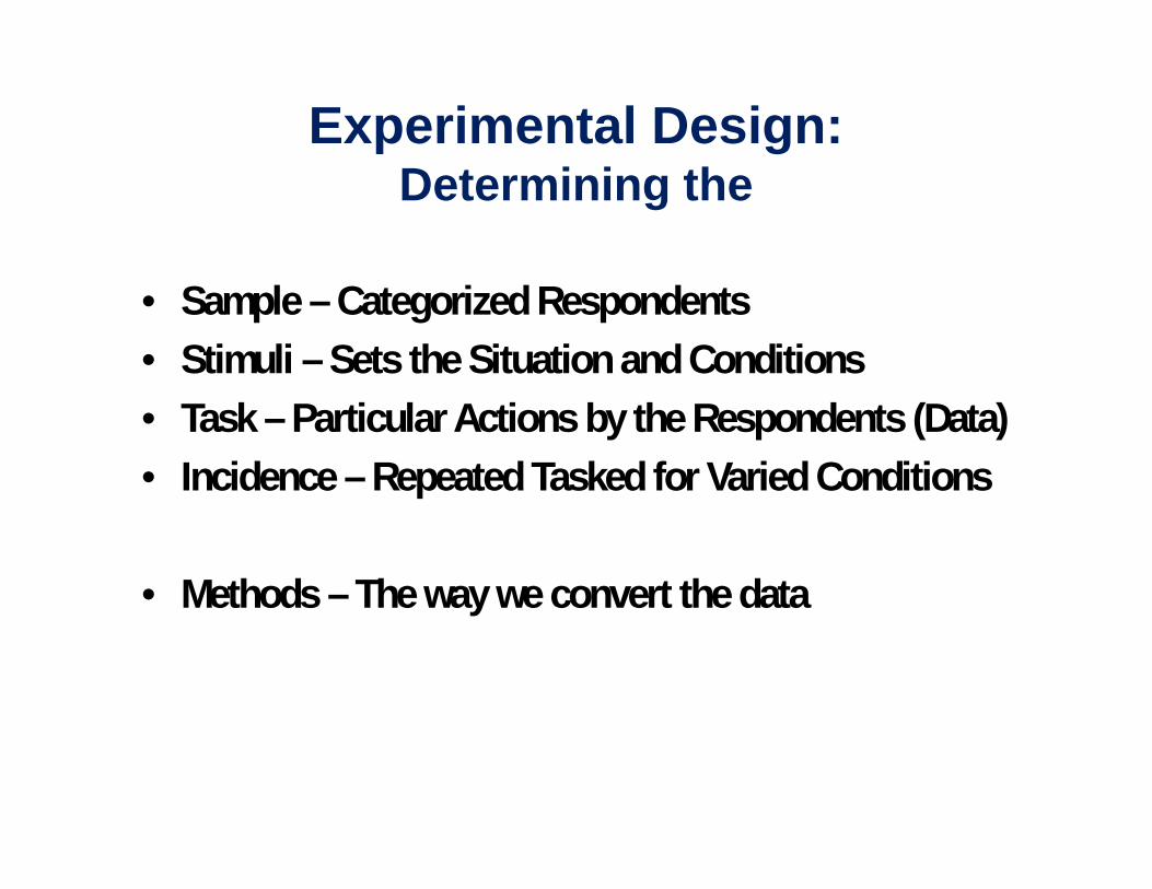
Experimental Design:Determining the

• Sample – Categorized Respondents• Stimuli – Sets the Situation and Conditions• Task – Particular Actions by the Respondents (Data)• Incidence – Repeated Tasked for Varied Conditions

• Methods – The way we convert the data

Variables (Stimuli & Respondents)• Target VariablesDirect EstimationMeasured for/with InteractionsMeasured with only Primary Effects

• Confounded VariablesNeed to Reduce the Variables Imposed Conditions Indirect Measurement with Assumed Relationship

• Nuisance “Unimportant”, Non-Drivers, ExtralitiesHandled Mainly by “Averaging”Unfortunately, they come back and bite your

Reality Check

• Do we capture the Process (Is it real?) Inclusion of VariablesCoverage of Variable RangesCoverage of Situations

• Is the Exercises Doable (without Undue Error)?• Is the Situation Believable?• Are the Results Meaningful?Consistency of InstructionsStability of Results Independence of Outside Conditions

Experimental Considerations• Coverage – Inclusion of Variables• Range – of the Variables and Conditions• Inherent Assumptions (Things Excluded)• Response Aggregation• Sensitivity of the Method (Fault Tolerance)• Difficulty of the Method• Efficiency of the Method• Quality of Responses• Flexibility – Ability to Modify Conditions with the Design• Robustness – Ability to Handle Partial, Incomplete, and Inaccurate

Data – Handling the Screw-ups• Reproducibility – Ability to Argument the Data

Quality & Validation• Data Quality Disengagement of Respondents (Straight-lining, randomization,

speeding, inconsistency) Projective Responses (Desirable Reactions) Confused Responses and Gaming Inappropriate Respondents

• Internal Validation (Consistency, Projective) Method Comparisons Internal Reference Testing (Hold-out Samples)

• External Validation (Predictive) References and Standard Problematic due to Scaling

• Face Validity Simulating The Process Context, Situation and Simplicity

Modeling the Market

MarketingCosts

CompetitivePricing

Costing Model Earnings Volumes &Revenue

EconomicDemandModel

The CompetitiveConsideration

Set

ManufacturingCosting Model

CustomerInput

Demand Curves and Functions

-40%

-20%

0%

20%

40%60%

80%

100%

120%

140%

Price

Sha

re

Probit/S-ShapedDemand

Linear

Modeling the Economic DemandLinear Demand Function

Volumea = + + ∑ { }

Volumea≥ 0

“S-Shaped” Demand Function

Sharea = Normal [ f ( + + ∑ { })]

f = stochastic function (Gaussian, Logistics)

Volumea = [ + ∑ { }] × Sharea (t = total)

Coefficients: estimated with regression

Test Variables: Pi (model levers)

Pricing Phenomena

• Optimum Product Pricing (Maximizing Earnings)• Joint Optimum Pricing (Multiple Products)• Optimum Reseller Pricing (Sales Margin)• Branding (Market Segmentation)• Optimum Product Design• Reaction of New Product Entry• Optimum Stochastic Pricing

www.lieb.com/Documents/PRICING5.pdf

New StandardPrice Estimate Previous Price

Product A $24.00 6.8% 0.0% $24.00Product B $20.00 1.1% 0.0% $20.00Product C $9.00 39.4% 37.9% $9.00Product D $20.00 0.5% 0.6% $20.00Product E $13.00 9.6% 13.6% $13.00Product F $7.00 28.0% 28.8% $7.00Product G $19.00 14.6% 19.1% $19.00

Cost EarningsProduct A $6.85 1.16Product E $5.00 0.77

Total 1.93

Share

Single Product Price Optimization

0%

10%

20%

30%

40%

50%

$4 $5 $6 $7 $8 $9 $10

Price

Shar

e

0%

20%

40%

60%

80%

100%

ShareProduct Earnings

Rela

tive

Earn

ings

LowPricePoint

High PricePoint

Optimum Price

Two Products Joint Pricing

22.

63.

2

3.8

4.4 5

5.6

6.2

6.8

7.4 8

22.6

3.23.8

4.455.6

6.26.8

7.48 Earnings

(% max)

Product B PriceP

rodu

ct A

Pri

ce

Two Supporting Products

95%-100%90%-95%85%-90%80%-85%75%-80%70%-75%65%-70%60%-65%55%-60%50%-55%

Methods of Measuring Demand• Market BasedEconometricsMarket Tests

• Value Based (www.lieb.com/Documents/PVALUE4.pdf)

Perceived Feature Value (Conjoint)Profiling (Simalto, “Build-Your-Own”Economic Value (Value-In-Use) (www.lieb.com/Documents/VALUE7.pdf)

• Direct Measurement (www.lieb.com/Documents/PRICING5.pdf)

Complete Choice ModelingConcept Testing (Gabor – Grender, Van Westendorp)

Complete Choice Pricing

• Direct Measure of Demand• Task: Respondents are asked “Intent to Purchase”

(or volume of purchase) from a “Consideration Set”of Options at various prices

• Stimuli: Consideration Set and the designed Prices• Incidence: Number of “Scenarios” at different

Prices

• Fairly easy exercise for the Respondent (Efficient)

Study: Materials for Photovoltaic Cells

The Problem as Given:• Measuring the choice of materials in the construction of Photovoltaic

Cells• Choice of four materials and the potential for Other.• And there are a number of Respondent variables (or descriptors.

The Design:• Three Materials will be Priced (the Fourth is Fixed)• See Eight Scenarios of varying prices.The Analysis:• Regression by Groups of Respondents: 5 equations with three

Dependent Variables

Study: Materials for Photovoltaic CellsOption Option 1 Option 2 Option 3 Option 4

StructureRack-Mounted

Traditonal RigidGlass Module;

Rack-Mounted Rigidlow weight Module

glass or filmfrontside

Rollabe PV affixesdirectly to substrate

Semiflex PV affixesdirectly to substrate

Current UseA $5.00 $8.00 $4.50 $6.79

% UsedB $5.00 $6.29 $5.16 $4.46

% UsedC $5.00 $4.57 $4.00 $7.64

% UsedD $5.00 $6.86 $5.66 $4.00

% UsedE $5.00 $4.00 $6.34 $6.40

% UsedF $5.00 $5.71 $6.88 $5.60

% UsedG $5.00 $5.14 $7.47 $5.12

% UsedH $5.00 $7.43 $8.00 $8.00

% Used

The Design• Three Varying Priced Options – One Fixed Price• Analysis will by Regression: How many scenarios: (# Variables + 1) x 2

(3 + 1) x 2 = 8 scenarios Series have to be “Orthogonal”; Inter-correlations ~ 0 (< 1%) Prices equally spaced Range Target Prices ± 50%

• Orthogonal Designs by Brute-Force Random Search for Initial Values Solver on Excel to find optimum solutions (Max. Correlation)

• Volumetric (% used) or Discrete Responses

Design Considerations• Meets the Method Requirements

(Orthogonally, Spacing, and Sample)• Meets the Phenomena Requirements

(Disaggregated Data on the Respondent Level)• Volumetric Data• Simple ExerciseQuality DataEfficiency – Note that this is one of five exercises in a Survey

• Face Validity• Internal Test of Consistency (R2)• Flexible – Not very robust

Data Aggregation• Data can be analyzed at the Respondent Level or

Aggregated If only single group aggregation is to be permitted, then

the data is handled as whole If groups of respondents are to be used, aggregation is

done on demand for analysis If an individual is required then analysis is down on the

respondent Level• Experimental Design allows for which type of

Aggregation

Study: Networked Laser Printers

The Problem as Given:• Measuring the choice of printers for Clustered Users (Small Businesses)• Choice of nine printers and the potential for Other.• And there are a number of Respondent variables.

The Design:• Five Levers (Three Printers, Two Brand Variations)• Twelve Scenarios of varying prices and Percentages.The Analysis:• Regression by Groups of Respondents: 10 equations with five

Dependent Variables

Network Laser MFP PrintersUS Version Printer Laser MFP (A)

Laser MFP(CM2320fxi)

Laser MFP(x546DTN)

Laser MFP(B)

Laser MFP(CM3530)

Laser MFP(x738) Laser MFP ©

Laser MFP(CM4540)

Laser MFP(x792)

Manufacturer Canon HP Lexmark Canon HP Lexmark Canon HP Lexmark Other

Unit Price $1,449 $985 $1,384 $2,236 $1,891 $2,657 $4,985 $3,388 $4,760

SelectionUnit Price $1,563 $1,500 $1,515 $2,345 $2,881 $2,908 $4,203 $5,161 $5,211

SelectionUnit Price $938 $1,226 $1,301 $2,018 $2,353 $2,498 $5,270 $4,216 $4,476


SelectionUnit Price $994 $1,121 $1,017 $2,673 $2,152 $1,952 $4,003 $3,856 $3,498


SelectionUnit Price $1,108 $938 $1,563 $2,891 $1,800 $3,000 $3,567 $3,225 $5,375

SelectionUnit Price $1,335 $1,353 $971 $3,000 $2,597 $1,864 $4,499 $4,654 $3,340




SelectionUnit Price $1,278 $1,274 $938 $1,800 $2,447 $1,800 $3,890 $4,384 $3,225

Selection

E

F

G

H

K

L

A

B

C

D

I

J

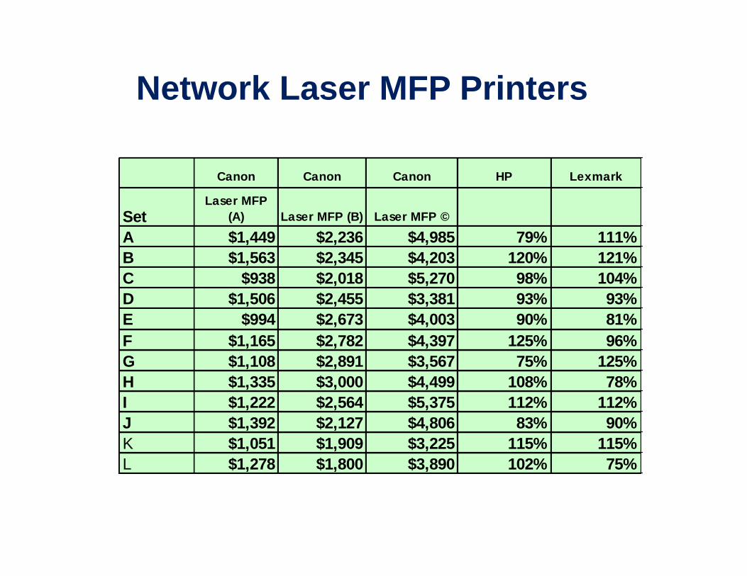
Network Laser MFP Printers

Canon Canon Canon HP Lexmark

SetLaser MFP

(A) Laser MFP (B) Laser MFP ©

A $1,449 $2,236 $4,985 79% 111%B $1,563 $2,345 $4,203 120% 121%C $938 $2,018 $5,270 98% 104%D $1,506 $2,455 $3,381 93% 93%E $994 $2,673 $4,003 90% 81%F $1,165 $2,782 $4,397 125% 96%G $1,108 $2,891 $3,567 75% 125%H $1,335 $3,000 $4,499 108% 78%I $1,222 $2,564 $5,375 112% 112%J $1,392 $2,127 $4,806 83% 90%K $1,051 $1,909 $3,225 115% 115%L $1,278 $1,800 $3,890 102% 75%

Design Considerations• Model is a linear combination of product prices,

percentage representing OEM Sources• Discrete Choice• Analysis is dictated by the Design• Meets the Method Requirements• Meets the Phenomena Requirements• More Complex ExerciseQuality Data ?Efficiency ?

• Face Validity

Study: Grain Combines

The Problem as Given:• Measuring the choice of Grain Combines by Growers and Processors• Choice of twelve machines & the potential for Other.• And there are a number of Respondent variables.

The Design:• Seven Levers (One Price, Four Percent Power Prices, Two Brand

Variations)• Sixteen Scenarios of varying prices and Percentages.The Analysis:• Regression by Groups of Respondents: 13 equations with seven

Dependent Variables

Study: Grain Combines85 HP 105 HP 125 HP 145 HP 165 HP 85 HP 105 HP 125 HP 145 HP 165 HP 85 HP 105 HP 125 HP 145 HP 165 HP Other

$51,000 $60,000 $65,000 $67,000 $74,000 $56,000 $67,000 $71,000 $74,000 $82,000 $53,000 $63,000 $67,000 $70,000 $77,000

$64,000 $68,000 $70,000 $85,000 $101,000 $77,000 $82,000 $85,000 $101,000 $122,000 $63,000 $67,000 $69,000 $83,000 $100,000

$59,000 $64,000 $69,000 $78,000 $78,000 $59,000 $64,000 $69,000 $78,000 $78,000 $51,000 $55,000 $59,000 $67,000 $67,000

$60,000 $69,000 $80,000 $92,000 $99,000 $65,000 $75,000 $86,000 $99,000 $106,000 $64,000 $73,000 $84,000 $97,000 $104,000

$58,000 $61,000 $71,000 $73,000 $78,000 $62,000 $66,000 $76,000 $78,000 $84,000 $57,000 $60,000 $69,000 $71,000 $77,000

$55,000 $60,000 $72,000 $80,000 $86,000 $59,000 $64,000 $77,000 $86,000 $92,000 $59,000 $63,000 $76,000 $85,000 $91,000

$69,000 $71,000 $83,000 $88,000 $104,000 $81,000 $84,000 $97,000 $104,000 $122,000 $67,000 $69,000 $80,000 $85,000 $100,000

$66,000 $66,000 $68,000 $68,000 $72,000 $70,000 $70,000 $72,000 $72,000 $76,000 $70,000 $70,000 $72,000 $72,000 $76,000

$57,000 $68,000 $73,000 $77,000 $91,000 $67,000 $80,000 $87,000 $91,000 $108,000 $57,000 $69,000 $74,000 $77,000 $92,000

$68,000 $81,000 $88,000 $92,000 $92,000 $68,000 $81,000 $88,000 $92,000 $92,000 $71,000 $84,000 $91,000 $96,000 $96,000

$52,000 $54,000 $57,000 $68,000 $72,000 $56,000 $57,000 $61,000 $72,000 $78,000 $60,000 $62,000 $65,000 $78,000 $83,000

$59,000 $68,000 $70,000 $80,000 $84,000 $62,000 $71,000 $73,000 $84,000 $89,000 $50,000 $58,000 $59,000 $68,000 $71,000

$56,000 $58,000 $58,000 $63,000 $71,000 $63,000 $66,000 $66,000 $71,000 $80,000 $57,000 $59,000 $59,000 $64,000 $72,000

$68,000 $82,000 $90,000 $105,000 $120,000 $78,000 $94,000 $103,000 $120,000 $137,000 $72,000 $86,000 $95,000 $110,000 $126,000

$55,000 $60,000 $70,000 $72,000 $87,000 $65,000 $72,000 $84,000 $87,000 $104,000 $50,000 $55,000 $64,000 $66,000 $79,000

$61,000 $65,000 $78,000 $90,000 $96,000 $66,000 $70,000 $84,000 $96,000 $103,000 $59,000 $63,000 $76,000 $87,000 $93,000

New Holland John Deere CASE

Study: Grain Combines

85 HP 105 HP (%) 125 HP (%) 145 HP (%) 165 HP (%) Deere (%) CASE (%)

SetA $51,000 118% 107% 104% 110% 104% 90%B $64,140 106% 104% 120% 120% 99% 90%C $59,100 108% 108% 113% 100% 86% 90%D $60,360 115% 115% 115% 108% 105% 94%E $58,200 105% 116% 103% 107% 98% 95%F $55,320 108% 120% 112% 107% 106% 98%G $69,000 103% 116% 107% 117% 97% 97%H $66,300 100% 102% 100% 106% 106% 99%I $56,760 119% 108% 105% 119% 101% 102%J $68,460 118% 109% 105% 100% 104% 103%K $52,260 103% 106% 119% 107% 115% 105%L $58,740 115% 103% 114% 105% 85% 108%M $56,040 104% 100% 108% 112% 102% 106%N $68,280 120% 110% 116% 114% 105% 105%O $54,600 110% 116% 104% 120% 91% 108%P $61,260 106% 120% 115% 107% 97% 110%

Design Considerations• Model is a linear combination of a product price,

percentage representing Power levels &percentages representing OEM Sources

• Discrete Choice• Analysis is dictated by the Design• Meets the Method Requirements• Meets the Phenomena Requirements• Much More Complex ExerciseQuality Data ?Efficiency ?

• Face Validity

Study: Packaged Software

The Problem as Given:• Measuring the choice of Software Grades, Source, Upgrade and Payment• Choice of fourteen Options• And there are a number of Respondent variables.

The Design:• Twelve Levers (Two Prices, One Dollar Premium, and Nine Percentage

Premiums)• Twenty-Six Scenarios of varying prices and percentages.• Split (Fragmented) SamplingThe Analysis:• Regression by Groups of Respondents: 14 equations with twelve

Dependent Variables

Study: Packaged SoftwareRetail

Set Professional SBE Standard Educational Professional SBE Standard StarOffice Professional SBE Basic Professional SBE Standard

A $593 $557 $499 $150 $362 $343 $292 $41 $311 $260 $208 $12.55 $11.80 $10.57B $349 $347 $344 $103 $234 $234 $231 $26 $134 $133 $130 $18.64 $18.53 $18.37C $505 $485 $475 $182 $357 $349 $334 $52 $239 $234 $224 $10.53 $10.11 $9.89D $272 $263 $251 $113 $179 $178 $166 $60 $141 $136 $122 $6.97 $6.75 $6.43E $255 $191 $156 $49 $188 $181 $108 $79 $164 $145 $69 $5.71 $4.27 $3.50F $210 $158 $115 $48 $121 $107 $65 $76 $93 $75 $45 $8.15 $6.14 $4.48G $179 $172 $165 $60 $131 $130 $122 $48 $96 $86 $75 $5.43 $5.23 $5.03H $366 $357 $339 $138 $273 $268 $254 $67 $140 $136 $119 $11.31 $11.00 $10.46I $428 $380 $298 $103 $285 $266 $211 $67 $271 $205 $94 $13.14 $11.66 $9.14J $523 $501 $488 $190 $293 $290 $269 $38 $231 $221 $182 $25.93 $24.87 $24.23K $608 $549 $442 $191 $415 $375 $286 $50 $328 $299 $207 $30.13 $27.22 $21.91L $411 $358 $304 $135 $278 $268 $192 $70 $274 $217 $91 $11.56 $10.05 $8.53M $245 $175 $98 $32 $176 $136 $62 $39 $147 $116 $30 $7.00 $5.01 $2.79N $199 $163 $142 $58 $134 $128 $91 $26 $86 $71 $49 $7.98 $6.55 $5.71O $504 $405 $324 $132 $327 $315 $207 $19 $409 $345 $150 $10.51 $8.46 $6.76P $147 $113 $59 $22 $111 $99 $41 $35 $118 $97 $27 $4.96 $3.82 $1.98Q $531 $484 $456 $151 $345 $329 $303 $47 $254 $242 $171 $19.06 $17.37 $16.39R $361 $346 $324 $118 $225 $222 $205 $37 $139 $133 $103 $7.83 $7.50 $7.01S $417 $338 $284 $90 $253 $251 $174 $70 $237 $203 $117 $15.45 $12.52 $10.54T $487 $418 $317 $121 $299 $282 $198 $52 $335 $281 $151 $16.28 $13.99 $10.61U $239 $230 $221 $99 $140 $135 $127 $37 $113 $105 $91 $6.31 $6.05 $5.81V $292 $281 $270 $97 $177 $171 $159 $79 $138 $127 $103 $8.62 $8.30 $7.95W $382 $284 $228 $94 $262 $237 $169 $34 $237 $166 $73 $11.20 $8.34 $6.69X $141 $104 $66 $21 $82 $65 $38 $50 $123 $93 $33 $4.51 $3.32 $2.11Y $575 $523 $469 $180 $354 $350 $284 $64 $223 $196 $169 $14.83 $13.51 $12.12Z $567 $506 $461 $172 $414 $391 $339 $59 $362 $305 $221 $31.52 $28.10 $25.60

Subscription (Monthly Charge)Retail Upgrade OEM

Study: Packaged SoftwareSet

ProfessionalPremium($)

SBEPremium(%)

StandardPrice($)

Education(%)

ProfessionalPremium (%)

SBEPreimum (%) Standard (%)

StarOffice($)

ProfessionalPremium (%)

SBEPremium(%

) Basic (%)Payback Time

(years)

A $94 62.5% $499 30.0% 75.0% 74% 58% $40.61 110% 50% 42% 3.94B $5 59.9% $344 30.0% 71.6% 94% 67% $25.67 82% 65% 38% 1.56C $30 35.0% $475 38.3% 74.1% 65% 70% $51.88 50% 68% 47% 4.00D $21 58.2% $251 45.0% 59.0% 96% 66% $60.48 90% 73% 49% 3.25E $99 35.0% $156 31.5% 80.0% 91% 69% $78.56 97% 81% 44% 3.72F $95 45.3% $115 41.3% 59.3% 75% 56% $75.80 50% 62% 39% 2.15G $13 50.6% $165 36.6% 61.8% 88% 74% $48.16 160% 52% 45% 2.74H $27 63.9% $339 40.7% 67.6% 72% 75% $67.09 76% 81% 35% 2.70I $130 63.0% $298 34.7% 56.7% 75% 71% $67.36 135% 63% 32% 2.72J $34 37.6% $488 39.0% 70.3% 90% 55% $38.40 145% 80% 37% 1.68K $166 64.6% $442 43.2% 78.1% 69% 65% $50.49 73% 76% 47% 1.68L $108 50.3% $304 44.5% 79.7% 88% 63% $70.30 170% 69% 30% 2.97M $147 52.6% $98 33.2% 77.2% 65% 64% $38.91 80% 74% 30% 2.91N $57 37.1% $142 40.8% 75.7% 86% 64% $26.09 64% 59% 35% 2.08O $180 45.2% $324 40.9% 66.7% 90% 64% $19.00 144% 75% 46% 4.00P $88 61.7% $59 36.8% 80.0% 83% 69% $35.07 103% 77% 46% 2.48Q $74 36.8% $456 33.2% 55.8% 62% 66% $46.72 112% 85% 38% 2.32R $38 59.7% $324 36.3% 55.0% 82% 63% $36.85 94% 85% 32% 3.85S $133 40.3% $284 31.8% 60.1% 97% 61% $70.07 90% 72% 41% 2.25T $169 59.7% $317 38.0% 60.1% 83% 62% $51.59 109% 71% 47% 2.49U $19 48.5% $221 45.0% 66.0% 60% 58% $36.59 118% 63% 41% 3.16V $23 52.6% $270 36.1% 79.4% 67% 59% $79.00 156% 67% 38% 2.83W $154 36.6% $228 41.1% 60.5% 73% 74% $34.25 107% 56% 32% 2.84X $75 50.3% $66 32.3% 58.8% 63% 57% $49.75 120% 66% 50% 2.61Y $105 51.4% $469 38.4% 66.7% 94% 60% $64.47 51% 50% 36% 3.23Z $107 42.2% $461 37.2% 69.7% 70% 74% $58.69 132% 60% 48% 1.50


percentage representing Versions, Sources,Discounts, Competition, and Payment Methods

• Discrete Choice• Analysis is dictated by the Design• Split Population (Merge Aggregation)• Meets the Phenomena Requirements• Even More Complex ExerciseQuality Data ?Efficiency ?

• Face Validity?

Study: Organizational Sales of Software

The Problem as Given:• Measuring the choice of Purchase Deal by Type of Software and

Payment• Choice of eleven Options• And there are a number of Respondent variables.

The Design:• Nine Levers (One Prices, Eight Percentage Options)• Sixteen Scenarios of varying prices and percentages showing quantity

Discounts. (Less than Required)The Analysis:• Regression by Groups of Respondents: 9 equations with eleven

Dependent Variables

Study: Organizational Sales of SoftwareNew 3D

PriceUpgrade to3D from Pro

Upgrade to3D from Std

CurrentLicense New Pro

Upgrade toPro from Pro

Upgradeto Pro

from Std New Std

Upgrade toStd from

StdNew

Elements

Upgradeto

Elements1-4 $944 $254 $287 $189 $387 $112 $125 $58 $17 $39 $295-49 $515 $139 $157 $103 $211 $61 $68 $32 $9+50 $412 $111 $125 $82 $169 $49 $54 $25 $71-4 $825 $289 $361 $166 $299 $69 $75 $187 $43 $39 $295-49 $356 $125 $156 $72 $129 $30 $32 $81 $19+50 $285 $100 $125 $57 $103 $24 $26 $64 $151-4 $986 $310 $310 $197 $251 $85 $91 $111 $38 $39 $295-49 $447 $140 $140 $89 $114 $39 $42 $50 $17+50 $358 $112 $112 $72 $91 $31 $33 $40 $141-4 $1,238 $402 $441 $271 $520 $201 $220 $254 $98 $39 $295-49 $636 $207 $226 $139 $267 $103 $113 $130 $50+50 $509 $165 $181 $111 $214 $82 $90 $104 $401-4 $1,259 $334 $364 $281 $447 $122 $133 $183 $50 $39 $295-49 $534 $141 $154 $119 $189 $52 $57 $78 $21+50 $427 $113 $123 $95 $152 $42 $45 $62 $171-4 $1,399 $432 $472 $336 $595 $221 $275 $182 $68 $39 $295-49 $630 $195 $213 $151 $268 $100 $124 $82 $30+50 $504 $156 $170 $121 $214 $80 $99 $65 $241-4 $1,252 $357 $434 $297 $435 $137 $171 $348 $109 $39 $295-49 $509 $145 $177 $121 $177 $56 $69 $142 $44+50 $408 $116 $141 $97 $142 $44 $56 $113 $361-4 $776 $194 $209 $192 $328 $106 $113 $230 $75 $39 $295-49 $291 $73 $78 $72 $123 $40 $42 $86 $28+50 $233 $58 $63 $58 $98 $32 $34 $69 $221-4 $972 $266 $328 $252 $374 $79 $95 $134 $28 $39 $295-49 $541 $148 $183 $140 $208 $44 $53 $75 $16+50 $433 $119 $146 $112 $167 $35 $42 $60 $131-4 $1,007 $277 $277 $265 $410 $87 $99 $320 $68 $39 $295-49 $549 $151 $151 $145 $224 $47 $54 $175 $37+50 $440 $121 $121 $116 $179 $38 $43 $140 $301-4 $909 $315 $342 $249 $455 $99 $113 $89 $19 $39 $295-49 $363 $126 $137 $99 $182 $40 $45 $35 $8+50 $290 $100 $109 $80 $145 $32 $36 $28 $61-4 $804 $259 $276 $235 $201 $62 $77 $86 $27 $39 $295-49 $416 $134 $143 $121 $104 $32 $40 $45 $14+50 $333 $107 $114 $97 $83 $26 $32 $36 $111-4 $699 $203 $235 $196 $273 $109 $125 $91 $36 $39 $295-49 $290 $84 $97 $81 $113 $45 $52 $38 $15+50 $232 $67 $78 $65 $90 $36 $41 $30 $121-4 $1,049 $347 $409 $290 $438 $173 $180 $339 $134 $39 $295-49 $590 $195 $230 $163 $246 $98 $101 $191 $76+50 $472 $156 $184 $130 $197 $78 $81 $153 $601-4 $1,273 $341 $425 $369 $382 $123 $123 $107 $34 $39 $295-49 $597 $160 $199 $173 $179 $58 $58 $50 $16+50 $477 $128 $159 $138 $143 $46 $46 $40 $131-4 $1,399 $456 $496 $420 $490 $98 $104 $255 $51 $39 $295-49 $606 $198 $215 $182 $212 $42 $45 $110 $22+50 $485 $158 $172 $145 $170 $34 $36 $88 $18

E

F

G

H

A

B

C

D

M

N

O

P

I

J

K

L

Study: Organizational Sales of Software

LowerPrice New 3D Price

Upgrade to 3Dfrom Pro

Upgrade to 3Dfrom Std

CurrentLicense New Pro

Upgrade to Profrom Pro

Upgrade toPro from

Std New Std

SetA 44% $944 27% 113% 20% 41% 29% 111% 15%B 35% $825 35% 125% 20% 36% 23% 109% 62%C 36% $986 31% 100% 20% 26% 34% 107% 44%D 41% $1,238 33% 110% 22% 42% 39% 110% 49%E 34% $1,259 27% 109% 22% 36% 27% 109% 41%F 36% $1,399 31% 109% 24% 43% 37% 125% 31%G 33% $1,252 29% 122% 24% 35% 31% 125% 80%H 30% $776 25% 108% 25% 42% 32% 106% 70%I 45% $972 27% 123% 26% 39% 21% 121% 36%J 44% $1,007 28% 100% 26% 41% 21% 114% 78%K 32% $909 35% 109% 27% 50% 22% 115% 20%L 41% $804 32% 107% 29% 25% 31% 125% 43%M 33% $699 29% 116% 28% 39% 40% 115% 33%N 45% $1,049 33% 118% 28% 42% 40% 104% 77%O 38% $1,273 27% 125% 29% 30% 32% 100% 28%P 35% $1,399 33% 109% 30% 35% 20% 106% 52%


percentage representing Versions, Sources,Discounts, and Payment Methods

• Discrete Choice• Analysis is dictated by the Design• Allow Disaggregation/ Respondent Level• Reduced Incidences (Reduced DF)• Complex ExerciseQuality Data ?Efficiency ?

• Face Validity?

Hierarchical Choice ExercisesReduced Consideration Set

• Choice Exercise Usually Reflect a SingleConsideration Set (Set of Completing/InteractingOptions)

• However, if you allow for multiple orderedselections (1st, 2nd, 3rd) choice, options can beremoved for analysis.

• For three ordered choices per scenario, you canremove up to two options from the exercise andrecomputed the selection.

• Starting with seven options, you can then represent29 combinations: all, removing any one, andremoving any two.

Take Away’s• The Results of the Research rests on the Quality of

the Experimental Design• Design Dictates the Analysis Model• No Perfect DesignAlways Balancing of Sources of ErrorHighly Conditional

• Designing Experiments is a Creative Process• It is Difficult and Requires Care