child expenditure: the role of working mothers, lone …anon-ftp.iza.org/dp388.pdf · ·...
TRANSCRIPT
IZA DP No. 388
Child Expenditure: The Role of Working Mothers,Lone Parents, Sibling Composition and HouseholdProvision
Lisa FarrellMichael A. Shields
DI
SC
US
SI
ON
PA
PE
R S
ER
IE
S
Forschungsinstitutzur Zukunft der ArbeitInstitute for the Studyof Labor
November 2001
Child Expenditure: The Role of Working Mothers, Lone Parents, Sibling Composition and Household Provision
Lisa Farrell Department of Economics, University of Melbourne
Michael A. Shields Department of Economics, University of Melbourne and IZA, Bonn
Discussion Paper No. 388 November 2001
IZA
P.O. Box 7240 D-53072 Bonn
Germany
Tel.: +49-228-3894-0 Fax: +49-228-3894-210
Email: [email protected]
This Discussion Paper is issued within the framework of IZA’s research area The Welfare State and Labor Markets. Any opinions expressed here are those of the author(s) and not those of the institute. Research disseminated by IZA may include views on policy, but the institute itself takes no institutional policy positions. The Institute for the Study of Labor (IZA) in Bonn is a local and virtual international research center and a place of communication between science, politics and business. IZA is an independent, nonprofit limited liability company (Gesellschaft mit beschränkter Haftung) supported by the Deutsche Post AG. The center is associated with the University of Bonn and offers a stimulating research environment through its research networks, research support, and visitors and doctoral programs. IZA engages in (i) original and internationally competitive research in all fields of labor economics, (ii) development of policy concepts, and (iii) dissemination of research results and concepts to the interested public. The current research program deals with (1) mobility and flexibility of labor markets, (2) internationalization of labor markets and European integration, (3) the welfare state and labor markets, (4) labor markets in transition, (5) the future of work, (6) project evaluation and (7) general labor economics. IZA Discussion Papers often represent preliminary work and are circulated to encourage discussion. Citation of such a paper should account for its provisional character.
IZA Discussion Paper No. 388 November 2001
ABSTRACT
Child Expenditure: The Role of Working Mothers, Lone Parents, Sibling Composition and Household Provision�
This paper uses detailed diary information from the British Family Expenditure Survey (FES) to investigate the expenditure patterns of school-age children. We estimate a Quadratic Almost Ideal Demand System, and find that, whilst most commodities are normal goods, sweets and toys are luxury items for children. Children of lone parents have lower budget shares for expenditure on soft drinks, leisure, personal goods and books/magazines, but higher budget shares for expenditure on sweets and vice products (alcohol, cigarettes and gambling). Having a working mother increases child expenditure on food products and toys. A higher parental budget share, on any given commodity, is generally associated with an increased child budget share suggesting that children mimic their parent’s expenditure patterns. JEL Classification: D11, D12, J13 Keywords: Child expenditure, quadratic almost ideal demand system, lone
parents, working mothers, sibling composition Michael Shields Department of Economics University of Melbourne Melbourne Victoria 3010 Australia Tel.: 006 13 8344 4656 E-mail: [email protected]
� We are grateful to Jeff Borland, Ken Clark, Rea Lydon, Ziggy MacDonald, Alan Duncan, Steve Pudney and Ian Walker for valuable comments. All remaining errors are our own.
1
I. Introduction
This paper extends our knowledge of children’s economic activity by investigating the
expenditure patterns of school-aged children. Expenditure pattern’s by young people is an under-
researched area.1 The scarcity of literature (exceptions include McNeal, 1987; and Warnaar and
van Praag, 1997) does not, however, imply that such behaviour is unimportant. It is clear that the
pattern of a child’s expenditure is an important aspect of her welfare. Furthermore child
expenditure does comprise a substantial proportion of the demand for the output of many
industries. For example, British children aged 7-15 spent, on average, £11.14 per week in 1998-
99, which multiplied by the number of children in that aged group, represented a total national
weekly expenditure of £671 million (or approximately a half of one-percentage of GDP).2
Today’s children are also the adult consumers of tomorrow and future expenditure patterns may
be affected by economic lessons experienced in childhood.
Much of the analyses regarding the economic behaviour of children has so far concentrated on
child incomes. The available evidence suggests that children begin to receive allowances (or
pocket money), in the sense of regular transfers from other household members, between the ages
of 5 and 7 years of age (Furnham and Thomas, 1984). The psychological and sociological
literature on the economic socialisation of children views the provision of such allowances as an
important element in teaching children how to use money and provides some familiarity with the
basic principles of exchange.
Child expenditure is especially interesting from an economic perspective given that children
are not constrained in the same way as adults by fixed costs such as housing. Thus a child’s
income is wholly disposable income,3 although the set of goods over which children allocate their
1 Whilst economists have considered the determinants of fertility (e.g. Becker, 1992), the economic costs to the household of children (see the references in Browning, 1992) and the role of children as suppliers of labour (e.g. Basu and Van, 1998), the child as a consumer has been largely neglected. 2 These figures are the authors own calculations based on 1991 Census data (6,027,377 children aged 7-15) and the average child expenditure figures gained for the nationally representative 1998-99 British Family Expenditure Survey used in this paper. 3 Although parents may impose saving schemes on children or influence how their children spend their income.
2
income is likely to be smaller than that of adults. Nevertheless there will be important differences
between children in their patterns of expenditures reflecting tastes and preferences as well as
economic and family circumstances. In this paper we estimate a complete demand system for
child expenditure in order to investigate how children spend their money. The system is estimated
using data from the 1998-99 British Family Expenditure Survey (FES), which contains detailed
expenditure information drawn from diaries completed by children over a two-week period. In
addition to controlling for child-specific characteristics (e.g. age, gender), we are also able to map
each child to their parental, sibling and other household characteristics.
This analysis allows us to investigate a number of important issues. Firstly, do lone parent
children have different expenditure patterns to children living with both parents? Does the low
income associated with lone parent households translate into lower children’s income and
expenditure, and do lone parent children consume a different bundle of goods to their two-parent
counterparts? In the latter respect, we are particularly interested in possible expenditure
differences on ‘unhealthy’ products such as sweets and vice (i.e. alcohol, cigarettes and
gambling). We believe that the answers to these questions are important for the welfare of the
growing numbers of lone-parent children in Europe and North America.
Secondly, recent decades have seen a sharp increase in the numbers of working mothers in
many countries. It is therefore of interest to examine whether or not this trend has impacted on
the expenditure activity of children. For example, are children of working mothers forced to be
more self-reliant at an earlier age, and therefore observed to have a higher budget shares for
expenditure on necessities such as food/snacks and drinks? Similarly, are children of working
mothers directly financially compensated for their mother being at work, and therefore observed
to have higher expenditures on ‘luxury’ goods such as toys, electrical goods and leisure
activities?
Thirdly, a number of recent papers have found that parents may favour boys when allocating
family resources. One suggested reason for this is that parents value children as an investment in
3
the sense that they are able to appropriate future earnings from them (see, for example, Deaton,
1989). If it is the case that, direct commodity market-interactions benefit children through an
educative process of economic socialisation, as well as through increased consumption, then we
might expect to see a gender bias directed towards higher expenditure activity among boys
relative to girls. Alternatively, it might be the case that adolescence, which is often argued to
occur earlier for girls than boys, may be associated with economic as well as physical and
emotional maturity in the eyes of parents. More generally, we would also expect to observe
gender-related differences in the types of goods which boys and girls purchase. We further
investigate this issue by looking at the gender composition of siblings (as well as the number of
siblings) given that siblings may act as a peer reference group for child expenditure patterns.
Fourthly, we are interested in the effect of age on expenditure patterns. We expect that total
expenditure will rise with age as allowances increase and the opportunity for income generation
outside the household expands. Moreover, the set of goods that children spend their money on is
likely to expand as the age of the child increases, reflecting changes in preferences and greater
purchase freedom from parental control. As children mature, we would expect to observe
children consuming relatively fewer ‘child-specific’ goods such as toys and sweets, and more of
the type of goods that are also consumed by adults.
Finally, we wish to explore if children’s expenditures reflect those of their parents.
Consideration of the pattern of children’s expenditure naturally leads us to ask how the allocation
of children’s resources is affected by household spending. For example, are child and parental
provision of commodities, complementary or substitute expenditures? Child expenditure need not
enhance child welfare if it merely acts as a substitute for parental provision. If the expenditure
patterns of children do mimic their parents, government policy initiatives aimed at promoting
healthier lifestyles and consumption patterns for today’s adults might lead to an improved future
consumption basket for tomorrow’s consumers. Given the uniqueness of our data source we are
able to investigate the above issues in some detail.
4
The paper proceeds as follows. Section II presents the consumer theory and the corresponding
statistical framework adopted for our analysis. In Section III we describe our data source and
highlight the expenditure patterns of the children in our sample. The results of the statistical
analysis are presented in Section IV, and we conclude the paper in Section V.
II. Consumer Theory and Statistical Framework
We are primarily interested in investigating how children’s budget shares differ across
commodity groups and how they vary with the child’s income and parental provision of goods,
controlling for individual heterogeneity. Recent evidence suggests that linear Engel curves might
not be appropriate for many goods (see Atkinson et. al., 1990; and Blundell, 1993). Linearity
implies that at the margin budget shares are independent of the level of expenditure. This is
unlikely to be true, as children from rich and poor households may not spend the same fraction of
a marginal unit of income on each commodity. We therefore, follow a recent paper by Banks et
al., 1997, and estimate a complete demand system for children’s expenditure, using a Quadratic
Almost Ideal Demand System (QUAIDS). In this specification the budget shares are quadratic in
the logarithm of income.
2.1. Quadratic Almost Ideal Demand System
Children are assumed to have preferences that are represented by the following utility function:
),...,( 21 njjjj cccUU � j=1,…,J (1)
Where ijc is the quantity of good i consumed by child j, and n is the number of goods
(commodity groups) such that, i=1,…,n. The basic budget share equation has the following
structure,
ijjijiiij yyw ���� ���� ])[(lnln 2 , i=1,…,n (2)
5
Where ijw = the budget share of commodity i, for child j, jy is the income level of child
j, iii ��� ,, are unknown parameters and ij� is a random error term.
Whilst we are looking at cross section data so that all children face the same prices, all
children do not face the same degree of household provision for each good. For some children
parents may provide some/many of the goods in an expenditure category. This may be especially
true of commodity groups like clothes and food/snacks. One of our principle research questions is
how parental expenditure affects child expenditure. We might anticipate that the more parents
spend on a given commodity group the less children will spend on that commodity group.
Alternatively, if children learn their expenditure habits through watching their parent’s
expenditure patterns then the opposite effect will occur, higher parental spending will be mirrored
by higher child spending for a given commodity group. For example, a number of studies have
found that the probability of an individual being a smoker or a drinker is positively related to
their parent’s consumption of these commodities (see, for example, MacDonald and Shields,
2001). This top down approach allows us to treat parental expenditure as exogenous. We are
implicitly assuming that children look at what their parents are providing and then decide how to
allocate their own income. We do not allow in this modelling framework for parental expenditure
to be influenced by how children spend their incomes. Whilst we accept that both effects may
exist we believe the former line of causation to be the dominant.4
Parental expenditure generates differentials in the supply of goods available from parental
contribution, across the commodity groups, which varies across children.5 We can therefore
include in our model a set of household budget shares for the child’s consumption set as follows:
4 Unfortunately it is not possible given our data to test the line of causation between parental provision and child expenditures. 5 This top down approach allows us to treat parental expenditure as exogenous. We are implicitly assuming that children look at what their parents are providing and then decide on how to allocate their own income. We do not allow in this modelling framework for parental expenditure to be influenced by how children spend their incomes. Whilst both effects might exisit we believe the former causation to be the dominant.
6
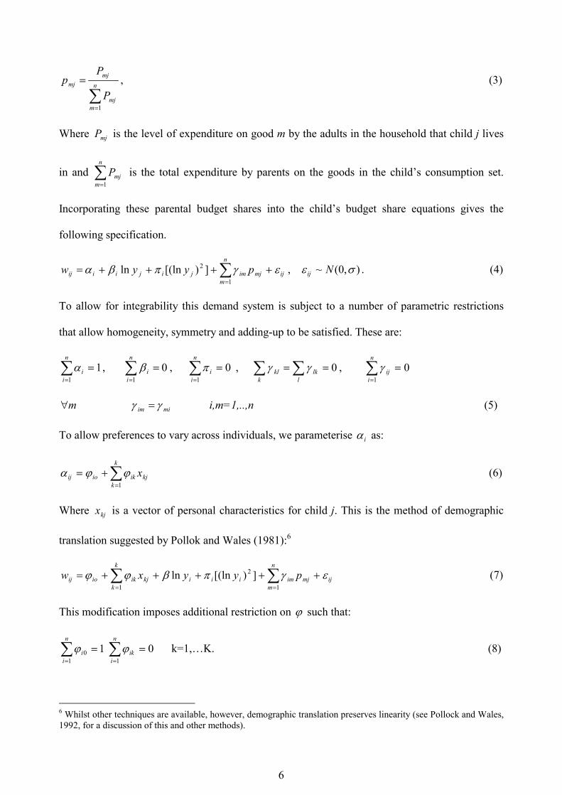
��
� n
mmj
mjmj
P
Pp
1
, (3)
Where mjP is the level of expenditure on good m by the adults in the household that child j lives
in and ��
n
mmjP
1
is the total expenditure by parents on the goods in the child’s consumption set.
Incorporating these parental budget shares into the child’s budget share equations gives the
following specification.
��
�����
n
mijmjimjijiiij pyyw
1
2 ])[(lnln ����� , ),0(~ �� Nij . (4)
To allow for integrability this demand system is subject to a number of parametric restrictions
that allow homogeneity, symmetry and adding-up to be satisfied. These are:
11
���
n
ii� , 0
1��
�
n
ii� , 0
1��
�
n
ii� , � � ��
k llkkl 0�� , 0
1
���
n
iij�
m� miim �� � i,m=1,..,n (5)
To allow preferences to vary across individuals, we parameterise i� as:
��
��
k
kkjikioij x
1��� (6)
Where kjx is a vector of personal characteristics for child j. This is the method of demographic
translation suggested by Pollok and Wales (1981):6
� �� �
������
k
k
n
mijmjimiiikjikioij pyyxw
1 1
2 ])[(lnln ������ (7)
This modification imposes additional restriction on � such that:
��
�
n
ii
10 1� �
�
�
n
iik
10� k=1,…K. (8)
6 Whilst other techniques are available, however, demographic translation preserves linearity (see Pollock and Wales, 1992, for a discussion of this and other methods).
7
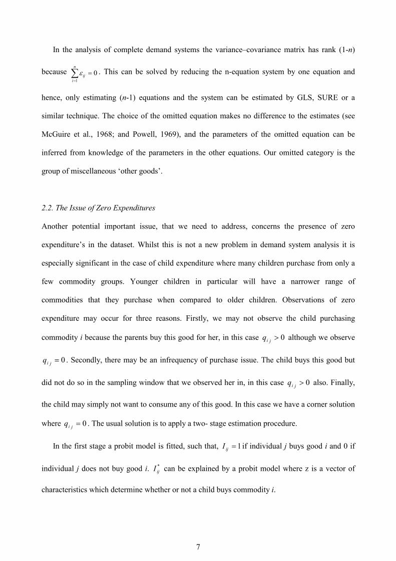
In the analysis of complete demand systems the variance–covariance matrix has rank (1-n)
because ��
�
n
iij
10� . This can be solved by reducing the n-equation system by one equation and
hence, only estimating (n-1) equations and the system can be estimated by GLS, SURE or a
similar technique. The choice of the omitted equation makes no difference to the estimates (see
McGuire et al., 1968; and Powell, 1969), and the parameters of the omitted equation can be
inferred from knowledge of the parameters in the other equations. Our omitted category is the
group of miscellaneous ‘other goods’.
2.2. The Issue of Zero Expenditures
Another potential important issue, that we need to address, concerns the presence of zero
expenditure’s in the dataset. Whilst this is not a new problem in demand system analysis it is
especially significant in the case of child expenditure where many children purchase from only a
few commodity groups. Younger children in particular will have a narrower range of
commodities that they purchase when compared to older children. Observations of zero
expenditure may occur for three reasons. Firstly, we may not observe the child purchasing
commodity i because the parents buy this good for her, in this case 0�jiq although we observe
0�jiq . Secondly, there may be an infrequency of purchase issue. The child buys this good but
did not do so in the sampling window that we observed her in, in this case 0�jiq also. Finally,
the child may simply not want to consume any of this good. In this case we have a corner solution
where 0�jiq . The usual solution is to apply a two- stage estimation procedure.
In the first stage a probit model is fitted, such that, 1�ijI if individual j buys good i and 0 if
individual j does not buy good i. *ijI can be explained by a probit model where z is a vector of
characteristics which determine whether or not a child buys commodity i.
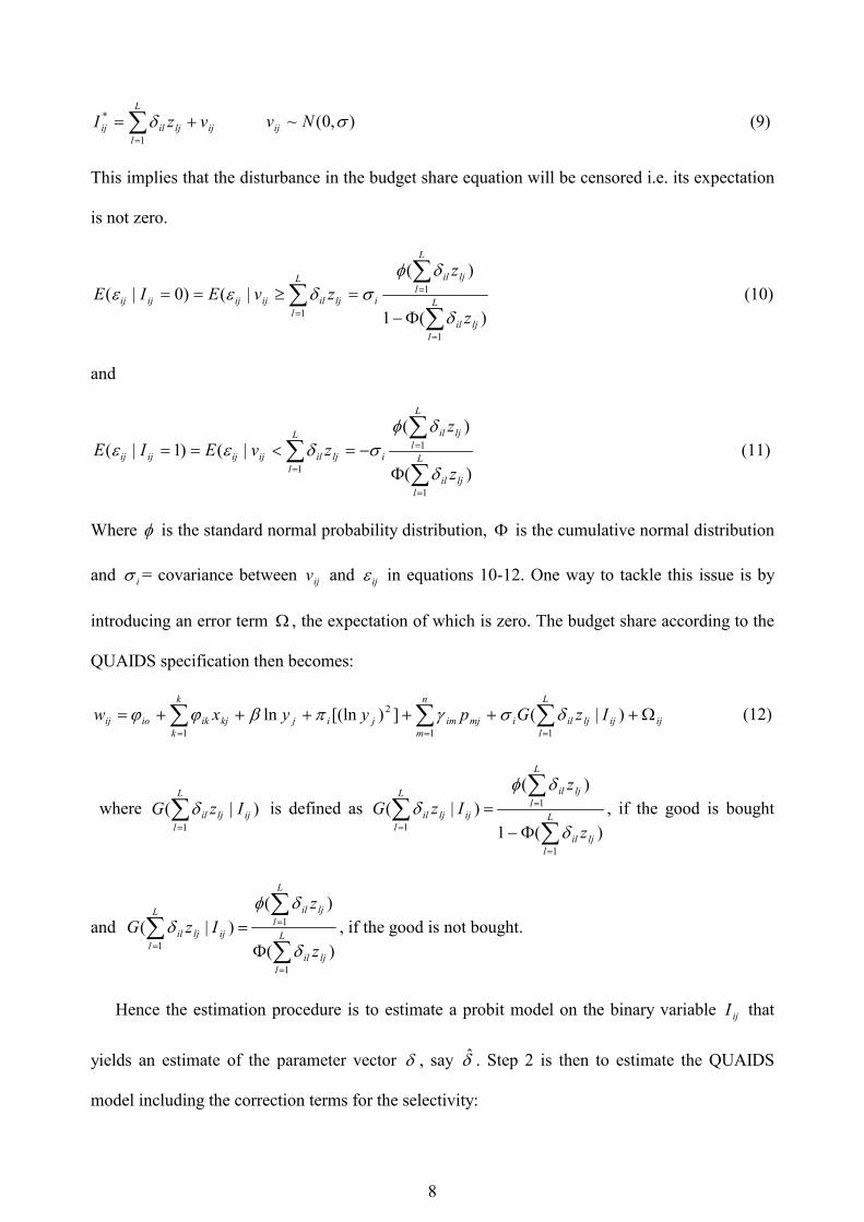
8
��
��
L
lijljilij vzI
1
*� ),0(~ �Nvij (9)
This implies that the disturbance in the budget share equation will be censored i.e. its expectation
is not zero.
��
�
�
�
�
��
����
L
lL
lljil
L
lljil
iljilijijijij
z
zzvEIE
1
1
1
)(1
)(|()0|(
�
��
���� (10)
and
��
�
�
�
�
�
�����
L
lL
lljil
L
lljil
iljilijijijij
z
zzvEIE
1
1
1
)(
)(|()1|(
�
��
���� (11)
Where � is the standard normal probability distribution, � is the cumulative normal distribution
and i� = covariance between ijv and ij� in equations 10-12. One way to tackle this issue is by
introducing an error term � , the expectation of which is zero. The budget share according to the
QUAIDS specification then becomes:
� � �� � �
��������
k
k
n
m
L
lijijljilimjimjijkjikioij IzGpyyxw
1 1 1
2 )|(])[(lnln ������� (12)
where ��
L
lijljil IzG
1)|( � is defined as �
�
�
�
�
�
��
�
L
lL
lljil
L
lljil
ijljil
z
zIzG
1
1
1
)(1
)()|(
�
��
� , if the good is bought
and ��
�
�
�
�
�
�
L
lL
lljil
L
lljil
ijljil
z
zIzG
1
1
1
)(
)()|(
�
��
� , if the good is not bought.
Hence the estimation procedure is to estimate a probit model on the binary variable ijI that
yields an estimate of the parameter vector � , say �̂ . Step 2 is then to estimate the QUAIDS
model including the correction terms for the selectivity:
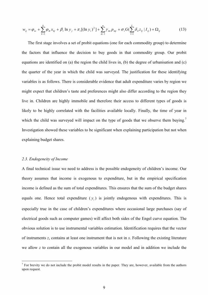
9
� � �� � �
��������
k
k
n
m
L
lijijljilimjimiijikjikioij IzGpyyxw
1 1 1
2 )|(])[(lnln ������� (13)
The first stage involves a set of probit equations (one for each commodity group) to determine
the factors that influence the decision to buy goods in that commodity group. Our probit
equations are identified on (a) the region the child lives in, (b) the degree of urbanisation and (c)
the quarter of the year in which the child was surveyed. The justification for these identifying
variables is as follows. There is considerable evidence that adult expenditure varies by region we
might expect that children’s taste and preferences might also differ according to the region they
live in. Children are highly immobile and therefore their access to different types of goods is
likely to be highly correlated with the facilities available locally. Finally, the time of year in
which the child was surveyed will impact on the type of goods that we observe them buying.7
Investigation showed these variables to be significant when explaining participation but not when
explaining budget shares.
2.3. Endogeneity of Income
A final technical issue we need to address is the possible endogeneity of children’s income. Our
theory assumes that income is exogenous to expenditure, but in the empirical specification
income is defined as the sum of total expenditures. This ensures that the sum of the budget shares
equals one. Hence total expenditure ( iy ) is jointly endogenous with expenditures. This is
especially true in the case of children’s expenditures where occasional large purchases (say of
electrical goods such as computer games) will affect both sides of the Engel curve equation. The
obvious solution is to use instrumental variables estimation. Identification requires that the vector
of instruments z, contains at least one instrument that is not in x. Following the existing literature
we allow z to contain all the exogenous variables in our model and in addition we include the
7 For brevity we do not include the probit model results in the paper. They are, however, available from the authors upon request.
10
child’s income by source (see Deaton, 1986; and Blundell et al., 1998,).8 This process is
described extensively in Charlier et al (2000, 2001). The children in our sample derive income
from a number of sources: allowances, gifts, earned income (both formal and informal), interest-
bearing deposits and savings.
Therefore we estimate an n commodity demand system with one equation omitted, because of
the singularity of the system. The equations estimated are those represented by equation 13
(which include the selection correction terms), so all equations contain the same explanatory
variables as is usual. The system is fitted by iterative 3 stage least squares (I3SLS) 9 given that
this allows us to estimate a system of structural equations where the equations contain
endogenous variables among the explanatory variables. This estimator uses an instrumental
variables approach to produce consistent estimates and generalised least squares (GLS) to
account for the correlation structure in the disturbances across equations. The key variables in the
Engel curves are the child’s income (defined as total expenditure) and the parental budget shares.
In addition, in order to investigate a number of issues raised in Section I we also control for child-
specific (i.e. gender, age, ethnicity), household (i.e. sibling composition, housing tenure and
council tax band10) and parental characteristics (i.e. lone parents, working mothers, father and
mothers age and education).
An alternative estimation approach would be to model child expenditure using a semi-
parametric framework that allows for greater flexibility in the modelling of the effect of income.
The approach adopted in recent papers focusing on adult expenditure patterns is to estimate semi-
parametric models separately for selected commodity groups (see Blundell et al, 1998). However,
we are unaware of any paper that has been able to estimate a complete demand system semi-
parametrically, even without controlling for the possible endogeneity of income or the excess 8 Further discussion of this issue can be found in the cited papers. 9 The resulting estimates have the same asymptotic properties as the ordinary three-stage least squares estimates (see Madansky, 1964). 10 Council tax bands are based on an evaluation of the value of your residential property, and are a nationally comparable measure. The bands range from A (lowest value home) to F (high value), and are likely to provide a reasonable proxy for wealth when also entered with housing tenure (i.e. renting, owner occupier etc.).
11
zero expenditures we have in our data.11 Although clearly not as flexible as a semi-parametric
framework, our model suggests that a quadratic specification for income adequately fits the data
thus accounting for the degree of Engel curvature correctly. Moreover Banks et al. (1997) show
that in practice the QUAIDS model does sufficiently well at capturing Engel curvature such that
additional semi-parametric terms are not required.
III. Data and Children’s Expenditure Patterns
This analysis is based on the little used data on children’s expenditure contained in the British
Family Expenditure Survey (FES). The FES is a nationally representative cross-sectional survey
that has been conducted on an annual basis since 1957. Some 10,000 households are selected
each year to take part in the FES, and the response rate is typically around 70%. The main aim of
the survey is to provide a reliable source of information on household expenditure, income and
other aspects of household finances. To account for seasonal differences in expenditure face-to-
face interviews are spread evenly over the year. Each individual aged 16 or over in the
households visited is asked to keep diary records of daily expenditure for two weeks. For the first
time in 1995-96 children aged between 7 and 15 were also asked to complete simplified diaries of
their daily expenditure. The children record only items that they purchase themselves with their
own money.12 The diaries are also confidential and therefore free of parental scrutiny which
might influence what the children record. In this paper we use the most recently released data
from the 1998-99 sweep of the survey. The response rate for the child diaries is exceptionally
high at 99%,13 giving us a sample of 1789 children aged 7 to 15 years.
11 See Banks et al, 1997, for a discussion of the problems of the impracticalities of semi-parametric and nonparametric methods in this context. 12 Items bought by an adult in a shop and then given directly to a child are not recorded as child expenditure. 13 The high response rate might in part be due to the fact that children are paid £5.00 for their efforts. This money is however given to the child at the end of the two- week period and should therefore not directly impact on their expenditure patterns during the time that we observe their behaviour. However, there may be some indirect bias if children spend more than their typically amounts as a result of the £5 payment they know that they will receive in the future.
12
The diaries give very detailed information on the expenditure patterns of children. By
matching the children to the household in which they live we are also able to obtain information
about the characteristics and composition of the household. We are, for reasons explained earlier,
especially interested in the effects of the economic position of the household and sibling
composition on children’s expenditure.
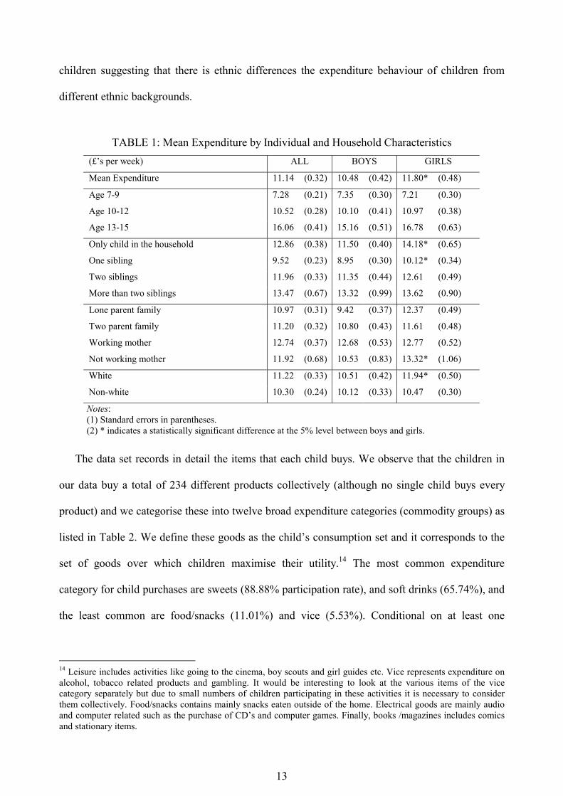
Table 1 reports the mean levels of expenditure by a number of child and household
characteristics. Note that we report the average weekly expenditures since the data is pre-
averaged over the two weeks the children keep the diary in an attempt to smooth expenditure
patterns and capture infrequent purchases. Children in our sample spend an average of £11.14 per
week, with the maximum amount spent by any one child being £180.21. As might be expected,
expenditure increases with the age of the child, with children aged 13-15 spending, on average,
over double the amount spend by those aged 7-9 (£16.06 compared to £7.28). Interestingly, the
girls in our sample record higher levels of expenditure activity than boys of around 12% (£11.80
compared to £10.48). There appears to be a non-linear relationship between number of siblings in
the household and expenditure. For both boys and girls, expenditure is highest for only-children
and those in large families (more than two siblings), and lowest for medium size families (one or
two siblings). An important issue, given the increasing numbers of lone-parent families in Europe
and North America, is whether children of lone parents have lower levels of expenditure that
children living with both parents. In this respect, the descriptive figures suggest that whereas
lone-parent boys have a lower average expenditure than their two-parent counterparts (£9.42
compared to £10.80), the converse is true for girls (£12.37 compared to £11.61). Children with
working mothers record higher levels of expenditure compared to children with mothers who
don’t work. However the break down across boys and girls shows that whilst the above is true for
boys, girls with working mothers have lower levels of expenditure when compared to girls with
mothers who do not working. Finally, white children record higher expenditure that non-white
13
children suggesting that there is ethnic differences the expenditure behaviour of children from
different ethnic backgrounds.
TABLE 1: Mean Expenditure by Individual and Household Characteristics (£’s per week) ALL BOYS GIRLS
Mean Expenditure 11.14 (0.32) 10.48 (0.42) 11.80* (0.48)
Age 7-9 7.28 (0.21) 7.35 (0.30) 7.21 (0.30)
Age 10-12 10.52 (0.28) 10.10 (0.41) 10.97 (0.38)
Age 13-15 16.06 (0.41) 15.16 (0.51) 16.78 (0.63)
Only child in the household 12.86 (0.38) 11.50 (0.40) 14.18* (0.65)
One sibling 9.52 (0.23) 8.95 (0.30) 10.12* (0.34)
Two siblings 11.96 (0.33) 11.35 (0.44) 12.61 (0.49)
More than two siblings 13.47 (0.67) 13.32 (0.99) 13.62 (0.90)
Lone parent family 10.97 (0.31) 9.42 (0.37) 12.37 (0.49)
Two parent family
Working mother
Not working mother
11.20
12.74
11.92
(0.32)
(0.37)
(0.68)
10.80
12.68
10.53
(0.43)
(0.53)
(0.83)
11.61
12.77
13.32*
(0.48)
(0.52)
(1.06)
White 11.22 (0.33) 10.51 (0.42) 11.94* (0.50)
Non-white 10.30 (0.24) 10.12 (0.33) 10.47 (0.30)
Notes: (1) Standard errors in parentheses. (2) * indicates a statistically significant difference at the 5% level between boys and girls.
The data set records in detail the items that each child buys. We observe that the children in
our data buy a total of 234 different products collectively (although no single child buys every
product) and we categorise these into twelve broad expenditure categories (commodity groups) as
listed in Table 2. We define these goods as the child’s consumption set and it corresponds to the
set of goods over which children maximise their utility.14 The most common expenditure
category for child purchases are sweets (88.88% participation rate), and soft drinks (65.74%), and
the least common are food/snacks (11.01%) and vice (5.53%). Conditional on at least one
14 Leisure includes activities like going to the cinema, boy scouts and girl guides etc. Vice represents expenditure on alcohol, tobacco related products and gambling. It would be interesting to look at the various items of the vice category separately but due to small numbers of children participating in these activities it is necessary to consider them collectively. Food/snacks contains mainly snacks eaten outside of the home. Electrical goods are mainly audio and computer related such as the purchase of CD’s and computer games. Finally, books /magazines includes comics and stationary items.
14
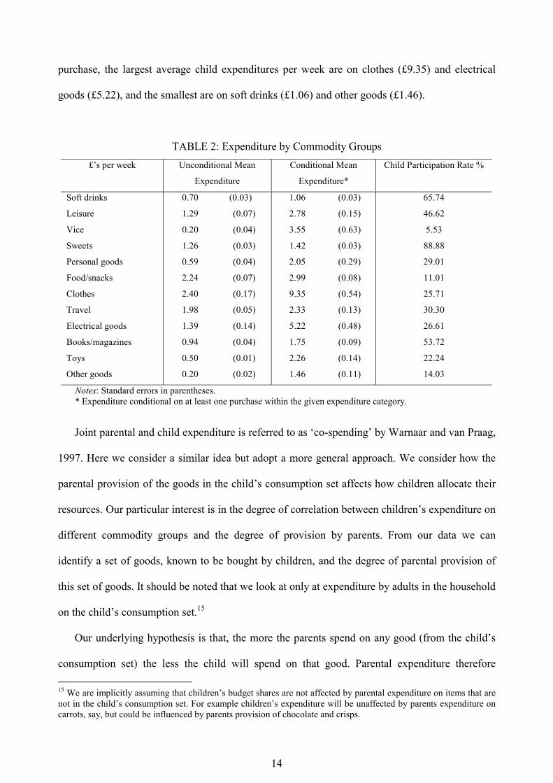
purchase, the largest average child expenditures per week are on clothes (£9.35) and electrical
goods (£5.22), and the smallest are on soft drinks (£1.06) and other goods (£1.46).
TABLE 2: Expenditure by Commodity Groups £’s per week Unconditional Mean
Expenditure
Conditional Mean
Expenditure*
Child Participation Rate %
Soft drinks 0.70 (0.03) 1.06 (0.03) 65.74
Leisure 1.29 (0.07) 2.78 (0.15) 46.62
Vice 0.20 (0.04) 3.55 (0.63) 5.53
Sweets 1.26 (0.03) 1.42 (0.03) 88.88
Personal goods 0.59 (0.04) 2.05 (0.29) 29.01
Food/snacks 2.24 (0.07) 2.99 (0.08) 11.01
Clothes 2.40 (0.17) 9.35 (0.54) 25.71
Travel 1.98 (0.05) 2.33 (0.13) 30.30
Electrical goods 1.39 (0.14) 5.22 (0.48) 26.61
Books/magazines 0.94 (0.04) 1.75 (0.09) 53.72
Toys 0.50 (0.01) 2.26 (0.14) 22.24
Other goods 0.20 (0.02) 1.46 (0.11) 14.03
Notes: Standard errors in parentheses. * Expenditure conditional on at least one purchase within the given expenditure category.
Joint parental and child expenditure is referred to as ‘co-spending’ by Warnaar and van Praag,
1997. Here we consider a similar idea but adopt a more general approach. We consider how the
parental provision of the goods in the child’s consumption set affects how children allocate their
resources. Our particular interest is in the degree of correlation between children’s expenditure on
different commodity groups and the degree of provision by parents. From our data we can
identify a set of goods, known to be bought by children, and the degree of parental provision of
this set of goods. It should be noted that we look at only at expenditure by adults in the household
on the child’s consumption set.15
Our underlying hypothesis is that, the more the parents spend on any good (from the child’s
consumption set) the less the child will spend on that good. Parental expenditure therefore 15 We are implicitly assuming that children’s budget shares are not affected by parental expenditure on items that are not in the child’s consumption set. For example children’s expenditure will be unaffected by parents expenditure on carrots, say, but could be influenced by parents provision of chocolate and crisps.
15
changes the effective prices (referred to as ‘pseudo-prices’ by Warnaar and van Praag, 1997) of
goods for children. We are, however, unable to tie this parental provision directly to children. It
might be that the adults consume the goods themselves. Moreover, for households with more than
one child we are unable to tie this adult expenditure to individual children. We simply look at the
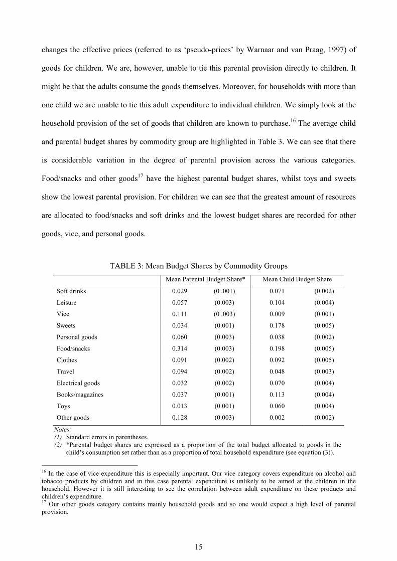
household provision of the set of goods that children are known to purchase.16 The average child
and parental budget shares by commodity group are highlighted in Table 3. We can see that there
is considerable variation in the degree of parental provision across the various categories.
Food/snacks and other goods17 have the highest parental budget shares, whilst toys and sweets
show the lowest parental provision. For children we can see that the greatest amount of resources
are allocated to food/snacks and soft drinks and the lowest budget shares are recorded for other
goods, vice, and personal goods.
TABLE 3: Mean Budget Shares by Commodity Groups Mean Parental Budget Share* Mean Child Budget Share
Soft drinks 0.029 (0 .001) 0.071 (0.002)
Leisure 0.057 (0.003) 0.104 (0.004)
Vice 0.111 (0 .003) 0.009 (0.001)
Sweets 0.034 (0.001) 0.178 (0.005)
Personal goods 0.060 (0.003) 0.038 (0.002)
Food/snacks 0.314 (0.003) 0.198 (0.005)
Clothes 0.091 (0.002) 0.092 (0.005)
Travel 0.094 (0.002) 0.048 (0.003)
Electrical goods 0.032 (0.002) 0.070 (0.004)
Books/magazines 0.037 (0.001) 0.113 (0.004)
Toys 0.013 (0.001) 0.060 (0.004)
Other goods 0.128 (0.003) 0.002 (0.002)
Notes: (1) Standard errors in parentheses. (2) *Parental budget shares are expressed as a proportion of the total budget allocated to goods in the
child’s consumption set rather than as a proportion of total household expenditure (see equation (3)).
16 In the case of vice expenditure this is especially important. Our vice category covers expenditure on alcohol and tobacco products by children and in this case parental expenditure is unlikely to be aimed at the children in the household. However it is still interesting to see the correlation between adult expenditure on these products and children’s expenditure. 17 Our other goods category contains mainly household goods and so one would expect a high level of parental provision.
16
IV. Empirical Results
We now turn to the empirical results from the QUAIDS model described in Section II. The
results from the model are generally consistent with our prior beliefs and earlier descriptive
analysis. The parameter estimates are presented in Table A1 in the Appendix. The first thing to
notice is the statistical significance of the correction terms in every equation. These indicate that
selection is an important issue in this context.18 This is entirely consistent with our prior beliefs
that each child will only be active in the consumption of goods from a few commodity groups.
Secondly the R-squared terms suggest the QUAIDS model fits the data well, ranging from 0.15
(electrical goods) to 0.49 (clothes). We start by discussing the influence of income in children’s
expenditure decisions by highlighting the estimated income elasticities associated with each
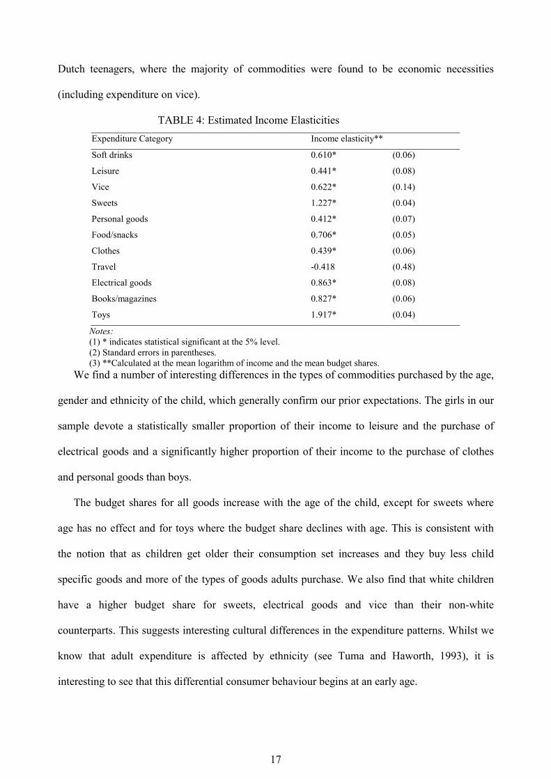
commodity group.19 The income elasticities, calculated at the mean logarithm of income and the
mean budget shares are shown in Table 4 and are statistically significant for all commodity
groups with the exception of travel20. Sweets and toys, both with elasticities greater than unity,
are found to be luxury goods for British children. In contrast, all other goods, including
expenditure on vice, are treated as necessities by children reflected in elasticities ranging from
0.441 for leisure and 0.412 for personal goods and, to 0.863 for electrical products and 0.827 for
books/magazines. The only exception is the negative elasticity found for travel expenditure,
which may be classed as an inferior good for children, although this result is not statistically
significant. These elasticities are similar to those found in Warnaar and van Praag (1997) for
18 This result is consistent with Warnaar and van Praag, 1997, who also found selection to be an important issue in the case of expenditure by Dutch teenagers. 19 These are calculated as wye iii /)ln2(1 �� ��� , where yln and w are the mean log of income and the mean budget share respectively. 20 The quadratic income terms in our model specification allow goods to be luxuries at some levels of income and necessities at others. We report the resultant income elasticities at the mean levels of income and at the mean budget shares.
17
Dutch teenagers, where the majority of commodities were found to be economic necessities
(including expenditure on vice).
TABLE 4: Estimated Income Elasticities Expenditure Category Income elasticity**
Soft drinks 0.610* (0.06)
Leisure 0.441* (0.08)
Vice 0.622* (0.14)
Sweets 1.227* (0.04)
Personal goods 0.412* (0.07)
Food/snacks 0.706* (0.05)
Clothes 0.439* (0.06)
Travel -0.418 (0.48)
Electrical goods 0.863* (0.08)
Books/magazines 0.827* (0.06)
Toys 1.917* (0.04)
Notes: (1) * indicates statistical significant at the 5% level. (2) Standard errors in parentheses. (3) **Calculated at the mean logarithm of income and the mean budget shares.
We find a number of interesting differences in the types of commodities purchased by the age,
gender and ethnicity of the child, which generally confirm our prior expectations. The girls in our
sample devote a statistically smaller proportion of their income to leisure and the purchase of
electrical goods and a significantly higher proportion of their income to the purchase of clothes
and personal goods than boys.
The budget shares for all goods increase with the age of the child, except for sweets where
age has no effect and for toys where the budget share declines with age. This is consistent with
the notion that as children get older their consumption set increases and they buy less child
specific goods and more of the types of goods adults purchase. We also find that white children
have a higher budget share for sweets, electrical goods and vice than their non-white
counterparts. This suggests interesting cultural differences in the expenditure patterns. Whilst we
know that adult expenditure is affected by ethnicity (see Tuma and Haworth, 1993), it is
interesting to see that this differential consumer behaviour begins at an early age.
18
Turning to household characteristics, we find a number of interesting relationships between
the type of housing the child lives in and their expenditure behaviour.21 We find that children
living in a local authority rented house (government provided) have lower budget shares for soft
drink, food/snacks, electrical goods and toys relative to children in our other housing categories,
and higher budget shares for clothes. Children living in a property that their parents own outright
have a significantly higher budget share for vice than other children. Living in a home owned by
your parents (mortgaged or owned outright) is associated with a higher budget share for sweets.
Generally, we find that the council tax band for the residential property is not a good indicator of
the relative budget share for most types of child expenditure. The only exceptions are for leisure
and personal goods where the budget share is higher for children living in highly valued
properties (band e/f and above).
Acting as proxies for household income these variables tentatively suggest that children from
wealthier households have higher budget shares for items which might be considered to be luxury
goods (electrical items, leisure activities and personal goods), whereas children living in the
poorest homes concentrate their expenditure on essential items such as clothing.
Household income is not included directly in our model as it is likely to be highly correlated
with the size of allowances given to children and thus with child expenditure.22 The correlation
between households wealth (indicated by the above proxy variables) and vice expenditures,
however, is especially interesting and suggests that it is children from wealthier households who
have the highest participation rates for vice commodities: defined here as smoking, drinking
alcohol and gambling.
Given the continuing concern about the increasing number of lone-parent children in Europe
and North America an important policy issue is whether lone-parent children have higher budget
21 As mentioned in Section II these variables are intended to be proxies for the level of wealth of the household. We do not include the household’s income directly because it is likely to be endogenous given that it is highly correlated with children’s allowances and hence their expenditures. 22 See Farrell and Shields (2001) for a full analysis of the determinants of child allowances.
19
shares for ‘less healthy’ commodities such as vice, and lower expenditure for ‘health enhancing’
commodities such as leisure and books/magazines (due to the associated low income of lone-
parent families). Our model clearly confirms this hypothesis with lone parent children being
found to have significantly lower budget shares for soft drinks, leisure, personal goods and
books/magazines, but higher budget share for vice expenditure. These results are consistent with
findings by Norton et al (1998) that living in a single-parent family is a very strong predictor of
adolescent drinking and smoking. There are obvious child welfare implications from these
results.
Next we consider the impact on child expenditure patterns of having a mother who goes out to
work. We find that having a working mother has a positive and significant effect on the budget
shares for food/snacks and toys. These results are consistent with the hypothesis that children of
working mothers are force to be more self-reliant (devoting higher budget shares to the provision
of food/snacks) and they may be financially compensated for their mothers being at work by
higher budget shares on toys. Alternatively, they may be devoting more resources to expenditure
on toys as a means of entertaining themselves in their mother’s absence. Unfortunately our data
does not allow us to investigate the validity of these plausible explanations.
One might expect parents to exert a significant influence over the way children spend their
money. To try to capture this effect we control for the level of schooling and age of the parents of
each child. We find that the budget shares for soft drinks, leisure, and travel fall with the years of
schooling of the father, but the budget share on vice increases. The education of the child’s
mother has a, perhaps surprising, negative impact on the budget share for books/magazines.
Fathers’ age impacts positively on the budget shares for travel and vice, and has a negative
impact on the budget shares for books/magazines. Finally having an older mother has a beneficial
positive impact on the demand for books/magazines and a negative impact on the demand for
leisure activities. Suggesting these children’s expenditure is more orientated towards educative
activities within the home.
20
An important issue is how the sibling composition of the household impacts on the consumer
behaviour of children, given that siblings may act as a peer reference group for children’s
expenditure. We find evidence that having a brother in the household increases the budget share
for food/snacks whilst having a sister reduces the budget share for food/snacks and soft drinks.
We also consider the effect of being a lone-child on demand patterns. The results show that lone
children have a lower budget share for travel, which maybe due to the fact that parents are less
happy to let children travel alone without the company of a sibling. Lone children are also found
to have higher budget shares for electrical goods and lower budget shares for books/magazines
than children living in larger families. This may suggest that they spend more of their income on
CD’s and computer game at the expense of the demand for books/magazines.
Finally, one of the main aims of this paper is to understand how parental expenditure patterns
impact on child expenditure. A key assumption that we make in our analysis is that parent’s
budget allocations are exogenous and not determined by child expenditures. As is typically found
for cross-equation effects in adult demand systems, we find that children do not generally take
into account the full set of parental budget shares when deciding on the allocation of resources to
a particular good (i.e. they may face ‘bounded rationality’). The cross equation effects of parental
provision are generally insignificant. Of the 25 (out of 110) that are statistically significant, 22
are positive, and only 3 are negative. Warnaar and van Praag, 1997, found similar results for
Dutch teenagers.
However, we do find strong evidence suggesting that children’s expenditure on any given
commodity is complementary to that of their parents. All of the own equation effects are positive
(except for parental provision toys) and four of the positive results are statistically significant at
the 5% level of significance, soft drinks, leisure, food/snacks, and electrical goods. At the ten
percent level of statistical significance parental provision of personal goods, clothes and
book/magazines are also significant. These results imply the greater the parental budget shares on
these goods the greater the child’s budget share. There is therefore a strong suggestion that
21
children mimic or learn from their parent’s expenditure patterns. This finding has important
implications for current government funded policy aimed at discouraging unhealthy lifestyles in
the current adult population, due to the potential beneficial impact on future generations
consumption behaviour.
V. Conclusion
In this paper we have provided new evidence on the expenditure behaviour of children. This is
achieved by using diary information on children’s expenditures collected as part of the 1998-99
British Family Expenditure Survey (FES). Child expenditure is very much an under-researched
topic in comparison to that of the determinants of fertility, the economic costs to the household of
children and the role of children as suppliers of labour. However, it is an important issue as
today’s children are the adult consumers of tomorrow and future expenditure patterns are likely to
be affected by economic lessons experienced in childhood. Moreover, children in our sample
spent, on average, £11.14 per week in 1998-99, which if multiplied by the number of children in
Britain in that aged group (i.e. 7-15), accounted for a total national weekly expenditure of £671
million. This expenditure comprises a substantial proportion of the demand for the output of
particular industries such as confectionary, toys and books/magazines. Both the psychological
and sociological literature on the economic socialisation of children view the provision of intra-
household transfer of money (in the form of allowances or pocket-money) and the corresponding
expenditure activity as an important element in teaching children how to use money and to
understand the basic principles of exchange.
Our empirical approach is a Quadratic Almost Ideal Demand System, which is estimated for
12 commodity groups frequently purchased by school-age children. Controlling for a number of
personal, sibling and household characteristics our main findings are that the estimated income
elasticities suggest that sweets and toys are ‘luxury’ goods for children, whilst all other
commodities are ‘necessities’ with elasticities ranging between 0.412 for personal goods and
22
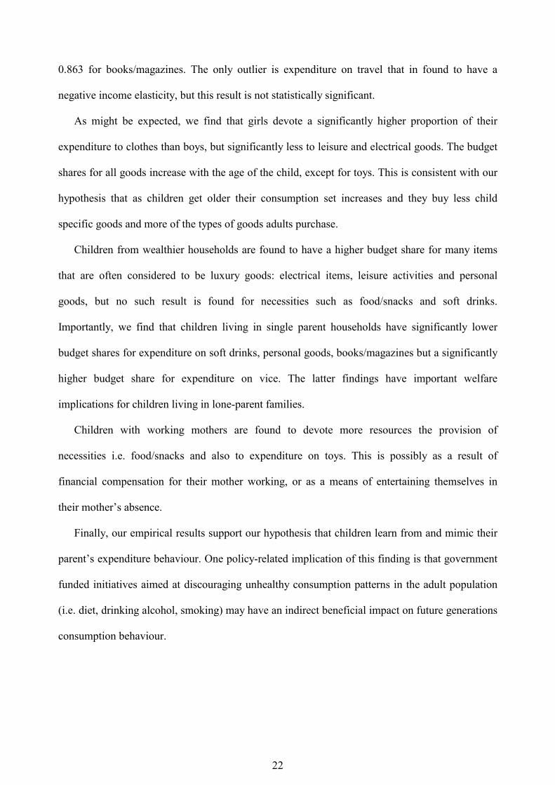
0.863 for books/magazines. The only outlier is expenditure on travel that in found to have a
negative income elasticity, but this result is not statistically significant.
As might be expected, we find that girls devote a significantly higher proportion of their
expenditure to clothes than boys, but significantly less to leisure and electrical goods. The budget
shares for all goods increase with the age of the child, except for toys. This is consistent with our
hypothesis that as children get older their consumption set increases and they buy less child
specific goods and more of the types of goods adults purchase.
Children from wealthier households are found to have a higher budget share for many items
that are often considered to be luxury goods: electrical items, leisure activities and personal
goods, but no such result is found for necessities such as food/snacks and soft drinks.
Importantly, we find that children living in single parent households have significantly lower
budget shares for expenditure on soft drinks, personal goods, books/magazines but a significantly
higher budget share for expenditure on vice. The latter findings have important welfare
implications for children living in lone-parent families.
Children with working mothers are found to devote more resources the provision of
necessities i.e. food/snacks and also to expenditure on toys. This is possibly as a result of
financial compensation for their mother working, or as a means of entertaining themselves in
their mother’s absence.
Finally, our empirical results support our hypothesis that children learn from and mimic their
parent’s expenditure behaviour. One policy-related implication of this finding is that government
funded initiatives aimed at discouraging unhealthy consumption patterns in the adult population
(i.e. diet, drinking alcohol, smoking) may have an indirect beneficial impact on future generations
consumption behaviour.
23
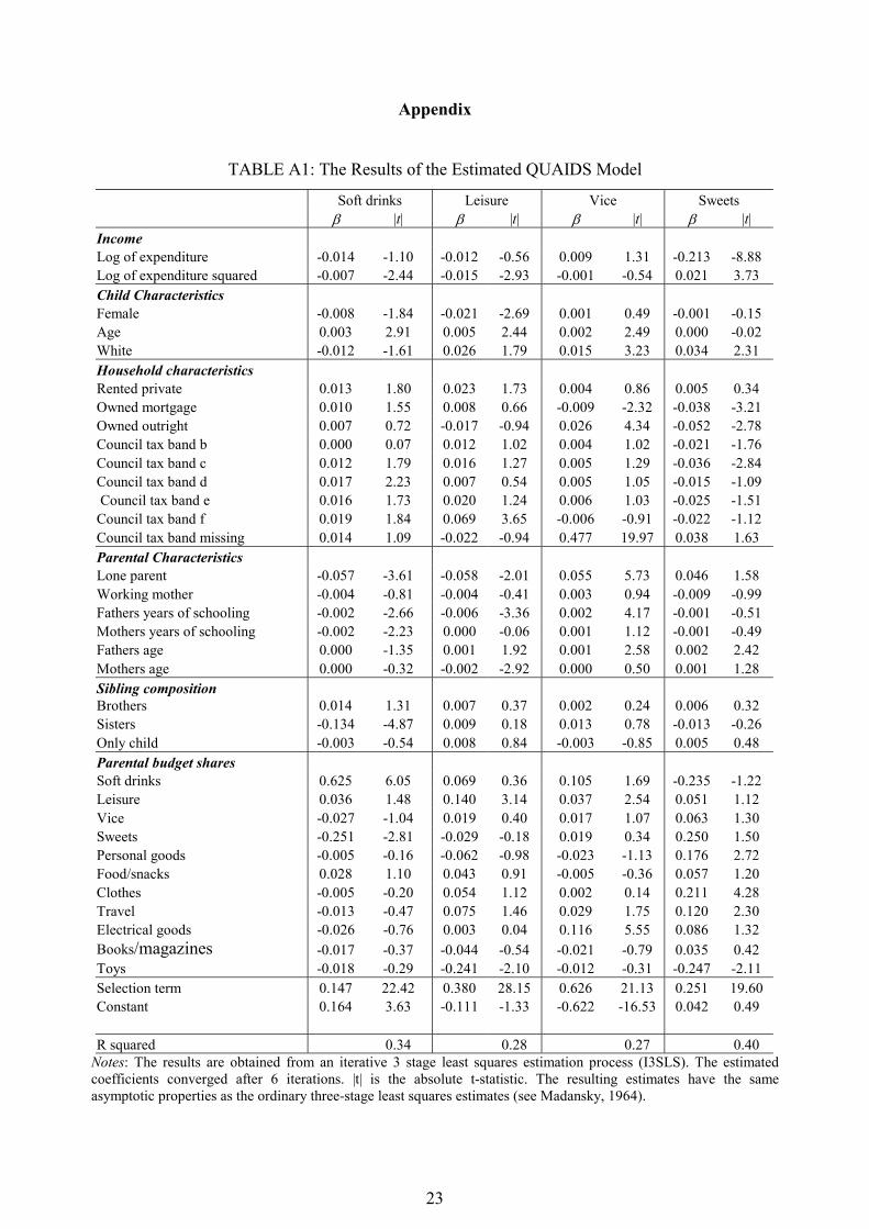
Appendix
TABLE A1: The Results of the Estimated QUAIDS Model
Soft drinks Leisure Vice Sweets � |t| � |t| � |t| � |t| Income Log of expenditure -0.014 -1.10 -0.012 -0.56 0.009 1.31 -0.213 -8.88 Log of expenditure squared -0.007 -2.44 -0.015 -2.93 -0.001 -0.54 0.021 3.73 Child Characteristics Female -0.008 -1.84 -0.021 -2.69 0.001 0.49 -0.001 -0.15 Age 0.003 2.91 0.005 2.44 0.002 2.49 0.000 -0.02 White -0.012 -1.61 0.026 1.79 0.015 3.23 0.034 2.31 Household characteristics Rented private 0.013 1.80 0.023 1.73 0.004 0.86 0.005 0.34 Owned mortgage 0.010 1.55 0.008 0.66 -0.009 -2.32 -0.038 -3.21 Owned outright 0.007 0.72 -0.017 -0.94 0.026 4.34 -0.052 -2.78 Council tax band b 0.000 0.07 0.012 1.02 0.004 1.02 -0.021 -1.76 Council tax band c 0.012 1.79 0.016 1.27 0.005 1.29 -0.036 -2.84 Council tax band d 0.017 2.23 0.007 0.54 0.005 1.05 -0.015 -1.09 Council tax band e 0.016 1.73 0.020 1.24 0.006 1.03 -0.025 -1.51 Council tax band f 0.019 1.84 0.069 3.65 -0.006 -0.91 -0.022 -1.12 Council tax band missing 0.014 1.09 -0.022 -0.94 0.477 19.97 0.038 1.63 Parental Characteristics Lone parent -0.057 -3.61 -0.058 -2.01 0.055 5.73 0.046 1.58 Working mother -0.004 -0.81 -0.004 -0.41 0.003 0.94 -0.009 -0.99 Fathers years of schooling -0.002 -2.66 -0.006 -3.36 0.002 4.17 -0.001 -0.51 Mothers years of schooling -0.002 -2.23 0.000 -0.06 0.001 1.12 -0.001 -0.49 Fathers age 0.000 -1.35 0.001 1.92 0.001 2.58 0.002 2.42 Mothers age 0.000 -0.32 -0.002 -2.92 0.000 0.50 0.001 1.28 Sibling composition Brothers 0.014 1.31 0.007 0.37 0.002 0.24 0.006 0.32 Sisters -0.134 -4.87 0.009 0.18 0.013 0.78 -0.013 -0.26 Only child -0.003 -0.54 0.008 0.84 -0.003 -0.85 0.005 0.48 Parental budget shares Soft drinks 0.625 6.05 0.069 0.36 0.105 1.69 -0.235 -1.22 Leisure 0.036 1.48 0.140 3.14 0.037 2.54 0.051 1.12 Vice -0.027 -1.04 0.019 0.40 0.017 1.07 0.063 1.30 Sweets -0.251 -2.81 -0.029 -0.18 0.019 0.34 0.250 1.50 Personal goods -0.005 -0.16 -0.062 -0.98 -0.023 -1.13 0.176 2.72 Food/snacks 0.028 1.10 0.043 0.91 -0.005 -0.36 0.057 1.20 Clothes -0.005 -0.20 0.054 1.12 0.002 0.14 0.211 4.28 Travel -0.013 -0.47 0.075 1.46 0.029 1.75 0.120 2.30 Electrical goods -0.026 -0.76 0.003 0.04 0.116 5.55 0.086 1.32 Books/magazines -0.017 -0.37 -0.044 -0.54 -0.021 -0.79 0.035 0.42 Toys -0.018 -0.29 -0.241 -2.10 -0.012 -0.31 -0.247 -2.11 Selection term 0.147 22.42 0.380 28.15 0.626 21.13 0.251 19.60 Constant 0.164 3.63 -0.111 -1.33 -0.622 -16.53 0.042 0.49 R squared 0.34 0.28 0.27 0.40
Notes: The results are obtained from an iterative 3 stage least squares estimation process (I3SLS). The estimated coefficients converged after 6 iterations. |t| is the absolute t-statistic. The resulting estimates have the same asymptotic properties as the ordinary three-stage least squares estimates (see Madansky, 1964).
24
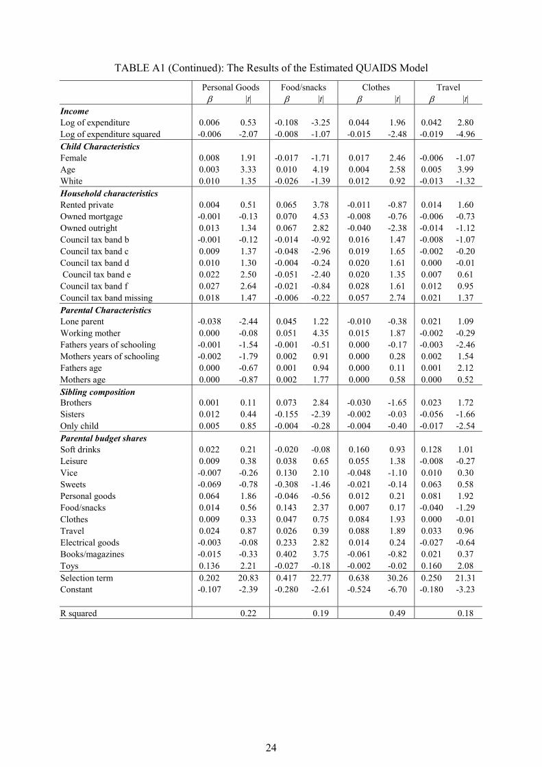
TABLE A1 (Continued): The Results of the Estimated QUAIDS Model
Personal Goods Food/snacks Clothes Travel � |t| � |t| � |t| � |t| Income Log of expenditure 0.006 0.53 -0.108 -3.25 0.044 1.96 0.042 2.80 Log of expenditure squared -0.006 -2.07 -0.008 -1.07 -0.015 -2.48 -0.019 -4.96 Child Characteristics Female 0.008 1.91 -0.017 -1.71 0.017 2.46 -0.006 -1.07 Age 0.003 3.33 0.010 4.19 0.004 2.58 0.005 3.99 White 0.010 1.35 -0.026 -1.39 0.012 0.92 -0.013 -1.32 Household characteristics Rented private 0.004 0.51 0.065 3.78 -0.011 -0.87 0.014 1.60 Owned mortgage -0.001 -0.13 0.070 4.53 -0.008 -0.76 -0.006 -0.73 Owned outright 0.013 1.34 0.067 2.82 -0.040 -2.38 -0.014 -1.12 Council tax band b -0.001 -0.12 -0.014 -0.92 0.016 1.47 -0.008 -1.07 Council tax band c 0.009 1.37 -0.048 -2.96 0.019 1.65 -0.002 -0.20 Council tax band d 0.010 1.30 -0.004 -0.24 0.020 1.61 0.000 -0.01 Council tax band e 0.022 2.50 -0.051 -2.40 0.020 1.35 0.007 0.61 Council tax band f 0.027 2.64 -0.021 -0.84 0.028 1.61 0.012 0.95 Council tax band missing 0.018 1.47 -0.006 -0.22 0.057 2.74 0.021 1.37 Parental Characteristics Lone parent -0.038 -2.44 0.045 1.22 -0.010 -0.38 0.021 1.09 Working mother 0.000 -0.08 0.051 4.35 0.015 1.87 -0.002 -0.29 Fathers years of schooling -0.001 -1.54 -0.001 -0.51 0.000 -0.17 -0.003 -2.46 Mothers years of schooling -0.002 -1.79 0.002 0.91 0.000 0.28 0.002 1.54 Fathers age 0.000 -0.67 0.001 0.94 0.000 0.11 0.001 2.12 Mothers age 0.000 -0.87 0.002 1.77 0.000 0.58 0.000 0.52 Sibling composition Brothers 0.001 0.11 0.073 2.84 -0.030 -1.65 0.023 1.72 Sisters 0.012 0.44 -0.155 -2.39 -0.002 -0.03 -0.056 -1.66 Only child 0.005 0.85 -0.004 -0.28 -0.004 -0.40 -0.017 -2.54 Parental budget shares Soft drinks 0.022 0.21 -0.020 -0.08 0.160 0.93 0.128 1.01 Leisure 0.009 0.38 0.038 0.65 0.055 1.38 -0.008 -0.27 Vice -0.007 -0.26 0.130 2.10 -0.048 -1.10 0.010 0.30 Sweets -0.069 -0.78 -0.308 -1.46 -0.021 -0.14 0.063 0.58 Personal goods 0.064 1.86 -0.046 -0.56 0.012 0.21 0.081 1.92 Food/snacks 0.014 0.56 0.143 2.37 0.007 0.17 -0.040 -1.29 Clothes 0.009 0.33 0.047 0.75 0.084 1.93 0.000 -0.01 Travel 0.024 0.87 0.026 0.39 0.088 1.89 0.033 0.96 Electrical goods -0.003 -0.08 0.233 2.82 0.014 0.24 -0.027 -0.64 Books/magazines -0.015 -0.33 0.402 3.75 -0.061 -0.82 0.021 0.37 Toys 0.136 2.21 -0.027 -0.18 -0.002 -0.02 0.160 2.08 Selection term 0.202 20.83 0.417 22.77 0.638 30.26 0.250 21.31 Constant -0.107 -2.39 -0.280 -2.61 -0.524 -6.70 -0.180 -3.23 R squared 0.22 0.19 0.49 0.18
25
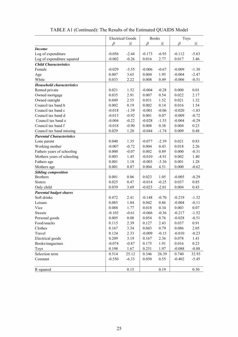
TABLE A1 (Continued): The Results of the Estimated QUAIDS Model
Electrical Goods Books Toys � |t| � |t| � |t| Income Log of expenditure -0.056 -2.44 -0.173 -6.93 -0.112 -5.63 Log of expenditure squared -0.002 -0.26 0.016 2.77 0.017 3.46 Child Characteristics Female -0.029 -3.55 -0.006 -0.67 -0.009 -1.30 Age 0.007 3.65 0.004 1.95 -0.004 -2.47 White 0.033 2.22 0.008 0.49 -0.006 -0.51 Household characteristics Rented private 0.021 1.52 -0.004 -0.28 0.000 0.01 Owned mortgage 0.035 2.91 0.007 0.54 0.022 2.17 Owned outright 0.049 2.55 0.031 1.52 0.021 1.32 Council tax band b 0.002 0.19 0.002 0.14 0.016 1.54 Council tax band c -0.018 -1.39 -0.001 -0.06 -0.020 -1.83 Council tax band d -0.013 -0.92 0.001 0.07 -0.009 -0.72 Council tax band e -0.004 -0.22 -0.028 -1.53 -0.004 -0.29 Council tax band f -0.018 -0.90 0.008 0.38 0.004 0.23 Council tax band missing 0.029 1.20 -0.044 -1.74 0.009 0.48 Parental Characteristics Lone parent 0.040 1.35 -0.077 -2.39 0.021 0.83 Working mother -0.007 -0.72 0.004 0.43 0.018 2.26 Fathers years of schooling 0.000 -0.07 0.002 0.89 0.000 -0.31 Mothers years of schooling 0.003 1.45 -0.010 -4.91 0.002 1.40 Fathers age 0.001 1.18 -0.003 -3.36 0.001 1.28 Mothers age 0.001 0.87 0.004 4.51 0.000 -0.62 Sibling composition Brothers 0.001 0.06 0.023 1.05 -0.005 -0.29 Sisters 0.025 0.47 -0.014 -0.25 0.037 0.85 Only child 0.039 3.69 -0.023 -2.01 0.004 0.43 Parental budget shares Soft drinks 0.472 2.41 -0.148 -0.70 -0.219 -1.32 Leisure 0.085 1.84 0.042 0.86 -0.004 -0.11 Vice 0.088 1.77 0.018 0.34 0.003 0.07 Sweets -0.103 -0.61 -0.066 -0.36 -0.217 -1.52 Personal goods 0.005 0.08 0.054 0.76 -0.028 -0.51 Food/snacks 0.115 2.39 0.127 2.43 0.037 0.91 Clothes 0.167 3.34 0.043 0.79 0.086 2.05 Travel 0.124 2.33 -0.009 -0.15 -0.010 -0.23 Electrical goods 0.209 3.19 0.167 2.36 0.078 1.41 Books/magazines -0.074 -0.87 0.175 1.91 0.016 0.23 Toys 0.198 1.67 0.251 1.97 -0.088 -0.88 Selection term 0.514 25.12 0.346 26.39 0.740 32.93 Constant -0.550 -6.33 0.050 0.55 -0.402 -5.45 R squared 0.15 0.19 0.30
26
References
Atkinson, A.B., Gomulka, J. and Stern, N.H. (1990). Spending on alcohol: Evidence from the
Family Expenditure Survey 1975-1983. Economic Journal, 100, pp. 808-827.
Banks, J., Blundell, R., and Lewbel, A. (1997). Quadratic Engel curves and consumer demand.
Review of Economics and Statistics, LXXIX, pp. 527-539.
Basu, K and Van P.H. (1998). The economics of child labour. American Economic Review, 88,
pp. 412-427.
Becker, G.S. (1992). Fertility and the economy. Journal of Population Economics, 5, pp. 185-
201.
Blundell, R., Duncan, A. and Pendakur, K. (1998). Semiparametric estimation and consumer
demand. Journal of Applied Econometrics, 13 pp534-461.
Blundell, R., Pashardes, P. and Weber, G. (1993). What do we learn about consumer demand
patterns from micro data?, The American Economic Review, 83, pp. 570-597.
Bradly, D.S. and Barber, H.A. (1948). The pattern of food expenditures. Review of Economics
and Statistics, 30, pp. 198-206.
Browning, M. (1992). Children and household economic behaviour. Journal of Economic
Literature, 30, pp. 1434-1475.
Charlier, E., Melenberg, B. and, van Soast, A.H.O. (2000). An anaylsis of housing expenditure
using semiparametric cross-section models. Empirical Economics,25, pp. 437-462.
Charlier, E., Melenberg, B. and, van Soast, A.H.O. (2001). An anaylsis of housing expenditure
using semiparametric models and panel data. Journal of Econometrics, 101, pp. 71-107.
Deaton, A. (1989), Looking for boy-girl discrimination in household expenditure data. World
Bank Review, 3, pp. 1-15.
Deaton, A. (1986). Demand analysis. In The Handbook of Econometrics, Vol III, Girliches, Z.,
and Intriligator, M.D. (eds). Elsevier Science Publishers BV.
Farrell, L. and Shields, M. (2001). Exploring the determinants of child allowances. Is there
evidence of gender bias? Mineo Department of Economics, University of Leicester.
Furnham, A.F. and Thomas, P. (1984). Pocket money: A study of economic education. British
Journal of Developmental Psychology, 2, pp. 205-212.
MacDonald, Z. and Shields, M. (2001). The impact of alcohol consumption on occupational
attainment in England. Economica, forthcoming.
Madansky, A. (1964). On the efficiency of three-stage least squares estimation. Econometrica,
32, pp. 51-56.
27
McGuire, T.W., Farley, R.W., Lucas, R. E., Winston, R.L. (1968). Estimation and inference for
linear models in which sub-sets of the dependant variable are constrained. Journal of the
American Statistical Association, 63, pp. 1201-1213.
McNeal, J.U. (1987). Children as Consumers: Insights and implications. Lexington, MA:
Lexington Books.
Norton, E.C., Lindrooth, R.C. and Ennett, S.T. (1998). Controlling for Endogoeneity of Peer
Substance Use on Adolescent Alcohol and Tobacco Use. Health Economics, 7 (5) pp 439-53.
Pollack, R.A. and Wales, T.J. (1981). Demographic variables in demand analysis. Econometrica,
49, pp. 1533-1551
Pollack, R.A. and Wales, T.J. (1992). Demand System Specification and Estimation. Oxford:
University Press.
Powel, A.A. (1969). Aitken estimators as a tool in allocating predetermined aggregates. Journal
of the American Statistical Association, 64, pp. 913-922.
Tuma, E.H., and Haworth B. (1993). Cultural diversity and economic education. Pacific Books.
Warnaar, M. and van Praag, B. (1997), How Dutch Teenagers spend their money. De Economist,
145, pp 367-397.
IZA Discussion Papers No.
Author(s) Title
Area Date
374
G. J. van den Berg B. van der Klaauw
Counseling and Monitoring of Unemployed Workers: Theory and Evidence from a Controlled Social Experiment
6 10/01
375
J. A. Dunlevy W. K. Hutchinson
The Pro-Trade Effect of Immigration on American Exports During the Late Nineteenth and Early Twentieth Centuries
1 10/01
376 G. Corneo Work and Television 5 10/01
377
S. J. Trejo
Intergenerational Progress of Mexican-Origin Workers in the U.S. Labor Market
1 10/01
378
D. Clark R. Fahr
The Promise of Workplace Training for Non-College-Bound Youth: Theory and Evidence from German Apprenticeship
1 10/01
379
H. Antecol D. A. Cobb-Clark
The Sexual Harassment of Female Active-Duty Personnel: Effects on Job Satisfaction and Intentions to Remain in the Military
5 10/01
380
M. Sattinger
A Kaldor Matching Model of Real Wage Declines
7 10/01
381
J. T. Addison P. Teixeira
The Economics of Employment Protection
3 10/01
382
L. Goerke
Tax Evasion in a Unionised Economy
3 11/01
383
D. Blau E. Tekin
The Determinants and Consequences of Child Care Subsidies for Single Mothers
3 11/01
384
D. Acemoglu J.-S. Pischke
Minimum Wages and On-the-Job Training
1 11/01
385
A. Ichino R. T. Riphahn
The Effect of Employment Protection on Worker Effort: A Comparison of Absenteeism During and After Probation
1 11/01
386
J. Wagner C. Schnabel A. Kölling
Threshold Values in German Labor Law and Job Dynamics in Small Firms: The Case of the Disability Law
3 11/01
387
C. Grund D. Sliwka
The Impact of Wage Increases on Job Satisfaction – Empirical Evidence and Theoretical Implications
1 11/01
388
L. Farrell M. A. Shields
Child Expenditure: The Role of Working Mothers, Lone Parents, Sibling Composition and Household Provision
3 11/01
An updated list of IZA Discussion Papers is available on the center‘s homepage www.iza.org.