chemistry in motion || fabrication by reaction–diffusion: curvilinear microstructures for optics...

6

Fabrication by

Reaction–Diffusion:

Curvilinear Microstructures

for Optics and Fluidics

6.1 MICROFABRICATION: THE SIMPLE

AND THE DIFFICULT

Miniaturization is the ‘arrow of time’ of modern technology. Computer chips, flat

panel displays, micromirror-based laptop projectors, RFID tags, inkjet valves,

microfluidic systems and countless other useful devices are all based on micro-

scopic components that are often invisible to the naked eye. To make such

structures, even the proverbial patience and precision of a Swiss watchmaker

would not be sufficient and new techniques (collectively known as microfabrica-

tion) are needed to manipulate, pattern and structure materials at the scale of

micrometers and below. Some of these techniques have achieved accuracy and

versatility that is simply breathtaking – for example, in microfabrication of

microelectronic components where a fully automated combination of photoli-

thography, vapor deposition and etching1,2 can produce microprocessors com-

prising hundreds ofmillions transistors with the overall process yield up to 93%.3,4

Yet, for some architectures, even the photolithographic wonders of Silicon Valley

may be inadequate. Photolithography is very efficient in delineating microstruc-

tures with ‘straight’ side walls (Figure 6.1(a)), but it is not readily extended to

curvilinear topographies (Figure 6.1(b)). In photolithography, it is easy to fully

Chemistry in Motion: Reaction–Diffusion Systems for Micro- and Nanotechnology Bartosz A. Grzybowski

© 2009 John Wiley & Sons Ltd. ISBN: 978-0-470-03043-1

UV-degrade/crosslink a polymer substrate beneath a ‘transparent/opaque’ photo-

lithographicmask and obtain a ‘binary’ surface relief, but it is hard to set up precise

gradients of light intensity to develop a curvilinear or multilevel surface profile.

Although one could try to make such structures via serial techniques (localized

electrodeposition,5 proton and ion beam machining,6,7 laser ablation,8 powder

blasting9 or electrochemical micromachining10), these procedures are usually

laborious, expensive and often unsuitable for very small structures. Luckily, there

is reaction–diffusion (RD). As we remember from earlier chapters, RD processes

are inherently linked with spatial concentration gradients. If we could somehow

control these gradients in space and time and translate them into local deformations

of a material supporting RD, we could fabricate such coveted nonbinary micro-

structures. In this chapter, we show how such translation can be achieved by

surprisingly simple experimental means.

Figure 6.1 (a) Cross-section of 64-bit high-performance microprocessor chip built inIBM�s 90 nm Server-Class CMOS technology. Though remarkably complex, PC micro-processors are nowadays manufactured in large quantities, and for as little as tens of dollars.(b) Surprisingly, fabrication of an apparently simple array of microlenses is more involved.A 2� 2 cm array can cost several hundred dollars. (a) Reprinted courtesy of InternationalBusiness Machines Corporation, � International Business Machines Corporation.

104 FABRICATION BY REACTION–DIFFUSION

6.2 FABRICATING ARRAYS OF MICROLENSES

BY RD AND WETS

Our first example of wet stamping (WETS) in action deals with arrays of micro-

scopic lenses for uses in optical data storage,11 imaging sensors,12 optical limiters13

and confocalmicroscopy14 to name just a few. Tomake these curvilinear structures

we will use an inorganic reaction between silver nitrate (AgNO3) and potassium

hexacyanoferrate (K4[Fe(CN)6]3), in which silver cations and hexacyanoferrate

anions precipitate according to 4Agþ þ [Fe(CN)6]4�!Ag4[Fe(CN)6] (#).

Importantly, it has been shown that if this precipitation occurs in a gelatin matrix,

it causes pronounced and permanent (i.e., persisting after the gel is dried) gel

swelling ofmagnitude linearly proportional to the amount of precipitate generated.15

This coupling between reaction products and gel dimensions/topography is central

to translating RD controllably into the shapes of the objects we wish to fabricate.

Our microfabrication process begins by placing a WETS stamp soaked in a

solution of AgNO3 and micropatterned in bas relief with an array of cylindrical

depressions (‘wells’) onto a thin film of dry gelatin uniformly loaded with K4Fe

(CN)6 (Figure 6.2(a)).When the surface of the stamp comes into conformal contact

with gelatin, water and ions diffuse from the stamp into the dry gel (Figure 6.2(b)

and Example 6.1). In doing so, the silver cations – constantly resupplied from the

stamp – precipitate all hexacyanoferrate anions they encounter and cause the gel to

swell. The interesting and relevant part of this process is the diffusion from the edges

of the circular features radially inwards (in the�r direction; Figure 6.2(b,c)). Here,as the reaction (precipitation) front propagates, the unreacted Fe(CN)6

4� experi-

ences a sharp concentration gradient at this front and diffuses in its direction – that is,

Figure 6.2 (a–c) Scheme of microlens fabrication using WETS. (d) Replication into apolymeric material cast against the lenses. (e) SEM (top) and optical (bottom) images of anarray of 50mm lenses replicated into PDMS. Reprinted from reference 17, with permission� 2005 American Institute of Physics.

FABRICATING ARRAYS OF MICROLENSES BY RD AND WETS 105

radiallyoutward (þ rdirection, red arrows inFigure6.2(b)). This ‘outflow’decreasesthe concentration of [Fe(CN)6]

4� anions near the circles� centers so that by the time

Agþ cations diffuse therein, they find fewer precipitation ‘partners’ than they had

near the patterned edges. In other words, the amount of precipitate and the degree of

gel swelling, z(r), both decreasemonotonically with decreasing r. The RD phenom-

ena continue until one of the reagents runs out. When RD comes to a halt, the

patterned regions are convex depressions in an otherwise flat surface (Figure 6.2(c)).

These depressions do not change shape when the gel is dried (drying only

compresses wet gelatin uniformly by �20%) and the developed topography can

bereplicated16intoothermaterials (e.g.,opticallytransparentpolydimethylsiloxane,

PDMS) to give regular arrays of convex microlenses that focus light efficiently

(Figure 6.2(d) and also insets to Figure 6.4(a)).17

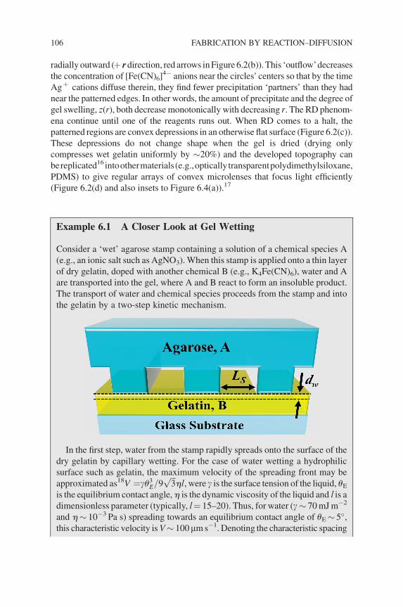
Example 6.1 A Closer Look at Gel Wetting

Consider a ‘wet’ agarose stamp containing a solution of a chemical species A

(e.g., an ionic salt such as AgNO3).When this stamp is applied onto a thin layer

of dry gelatin, doped with another chemical B (e.g., K4Fe(CN)6), water and A

are transported into the gel, where A and B react to form an insoluble product.

The transport of water and chemical species proceeds from the stamp and into

the gelatin by a two-step kinetic mechanism.

In the first step, water from the stamp rapidly spreads onto the surface of the

dry gelatin by capillary wetting. For the case of water wetting a hydrophilic

surface such as gelatin, the maximum velocity of the spreading front may be

approximated as18V ¼gu3E=9ffiffiffi3

phl, were g is the surface tension of the liquid, uE

is the equilibrium contact angle,h is the dynamic viscosity of the liquid and l is adimensionless parameter (typically, l¼ 15–20). Thus, for water (g� 70mJm�2

and h� 10�3 Pa s) spreading towards an equilibrium contact angle of uE� 5�,this characteristic velocity isV� 100mms�1. Denoting the characteristic spacing


between the edges of the stamp�s microfeatures by Ls (typically �100–500mmfor the examples discussed in this chapter), the characteristic time of the wettingprocess may be estimated as twet� Ls/V� 1–5 s.

Whereas wetting hydrates the surface layer of gelatin rapidly, water transport

into the bulk of the dry gel proceeds slowly by a diffusive process characterized

by a diffusion coefficient,Dw� 10�7 cm2 s�1.19Meanwhile, species A andB are

free to diffuse (with typical diffusion coefficient Ds� 10�5 cm2 s�1) and react

within the hydrated portion of the gel. The characteristic time required to form

anyRDpatterns/structures over distanceLs is tdiff � L2s=Ds � 10--250 s. During

this time, water diffuses a distance dw� (tdiffDw)1/2� 10–50mm into the bulk of

the gel. Importantly, the initial water transport into the gel may be consideredindependent of that of the chemical species, A, which is effectively ‘filtered’from the water due to its reactive consumption by species B. With theseconsiderations, one may treat RD phenomena as occurring in a thin (�10–50mm)layer of a hydrated gel. This approximation allows us to neglect migration ofwater within the substrate and variation of diffusion coefficients of salts with geldepth. These simplifications make theoretical treatment of our RD systemsconsiderably easier, and we will use them frequently throughout the book.

For the RD fabrication to be truly useful, it should, as mentioned in Chapter 1,

allow for the ‘programming’ of the shapes and curvatures of the lenses one wishes

to prepare. Since local deformations of the gel surface depend on the underlying

concentrations of the precipitate, the shapes of the developed lenses can be

controlled by the concentrations of the salts used and/or the dimensions of the

stamped features. Trends based on experimental surface profilograms (Figure 6.3)

illustrate how the depth, Ld, of the lenses changes with changing [AgNO3],

[K4Fe(CN)6] and the diameter of the stamped features, d.

For a given value of d and with [AgNO3] kept constant, Ld increases with

increasing [K4Fe(CN)6] (up to 1%w/w; above this concentration, the gelatin does

not gelate properly and tends to ‘melt’ upon stamping). This trend (Figure 6.3(a))

reflects the fact that when more potassium hexacyanoferrate is available in the

patternedfilm, themore precipitate can form, and the higher the degree of swelling.

At the same time, increasing the concentration of K4Fe(CN)6 decreases the

effective diameter of the lens, d 0, and increases the surface curvature. These

effects can be explained by the extent of the propagation of the precipitation front

inwards: when [K4Fe(CN)6] is low, all ions are precipitated below or in the vicinity

of the stamped ring and only these regions develop curvature; when more

hexacyanoferrate is available, the front travels further, curving the center of the

circle and leaving behind itself a flat region of uniform precipitation.

When d and [K4Fe(CN)6] are kept constant (Figure 6.3(b)), Ld increases with

increasing [AgNO3] up to�10%w/w concentration, but the lenses are relatively

flat-bottomed. Curved lenses approximated by sections of a sphere are obtained

FABRICATING ARRAYS OF MICROLENSES BY RD AND WETS 107

for [AgNO3] > 10%. In this regime, however, Ld decreases with increasing

concentration of silver nitrate. This trend is due to ‘flooding’ of the gelatin with a

large amount of AgNO3, so that the reaction front reaches the center of a lens

rapidly, precipitates the Fe(CN)64� still present therein and lifts this region up

with respect to the perimeter of the lens.

Finally, for given concentrations of the participating chemicals, Ld increases

with increasing diameter of the stamped circles d (Figure 6.3(a,b)) until it plateaus

Figure 6.3 (a) Experimental dependence of the depth, Ld, of circularly symmetricdepressions on feature size, d, for varying concentrations of K4Fe(CN)6 in gelatin(*, 0.25%; &, 0.5%; *, 0.75%; &, 1.0%) and for a constant concentration of AgNO3 inthe stamp (10%). Inset shows the same data plotted against [K4Fe(CN)6] for different valuesof d (*, 50 mm; &, 75mm; *, 100mm; &, 150mm). (b) Ld as a function of d for[K4Fe(CN)6]¼ 1% w/w and for variying [AgNO3] (&, 5%; *, 10%; *, 15%; &, 20%).Inset shows the same data plotted against [AgNO3] for different values of d(*, 50mm; &, 75mm; *, 100mm; &, 150 mm). Graphs in (a) and (b) were created basedon profilometric measurements of the gelatin masters. Standard deviations of Ld werecollected from at least three independent stampings and two profilometric scans (averagedover ten times each) spanning two to five features for each stamping. For lenses withd < 100 mm, standard deviations were less than 1%. (c, d) Dependencies of Ld on dmodeledusing the lattice gasmethod and corresponding to the experimental trends in, respectively, (a)and(b).Theunitsonbothaxesarearbitrarybut linearlyproportional to theexperimentalones–thatis,in(c),relativeconcentrationsforcurves*:&:*:&¼ 1:2:3:4;in(d)&:*:&:*¼ 1:2:3:4.For further details, see Ref. 17 (Reprinted with permission fromAppl. Phys. Lett. (2004), 85,1871.� 2005 American Institute of Physics.)


at d� 150–200 mm. In this limit, the precipitation front from the perimeter ofthe circle does not propagate all the way to the circle�s center (remember thatdiffusive transport `slows down'with distance traveled), andLd depends only on thedegree of swelling directly below the features. In addition, increasing d decreases

the curvature of the lenses: in large circles, the central area where no precipitation

occurred remains flat.

The technique can be straightforwardly extended to arrays of microlenses of

arbitrary base shapes. Figure 6.4 shows optical micrographs of ‘pyramidal’ lenses

obtained bywet stamping arrays of triangles (Figure 6.4(a)), squares (Figure 6.4(b)),

hexagons (Figure 6.4(c)) and stars (Figure 6.4(d)). As in the case of circularly

symmetric patterns, the topographic details of these reliefs can be controlled by the

concentrations of the participating chemicals, and can be faithfully reproduced into

optically useful polymers.

6.3 INTERMEZZO: SOME THOUGHTS ON

RATIONAL DESIGN

Our method�s sensitivity to the RD process parameters (salt concentrations and

dimensions of the stamped features) is in some sense a double-edged sword. On

the one hand, by changing these parameters we can fabricate a continuum of

microlens shapes (hemispheres, ‘copulas’ of different curvatures, pyramids,

etc.); on the other hand, we cannot readily guess a priori the values of

parameters that would produce a particular lens (say, a section of sphere with

Ld¼ 20 mm and diameter d¼ 600 mm). Of course, we could standardize themethod by recording the experimental trends (such as those described inSection 6.2) for different parameter values, and then extrapolate/approximatethe values needed to build a desired structure. This brute-force approach,however, would be time-consuming and laborious and would certainly detractfrom the appeal of supposedly `effortless' RD fabrication. The more rationalapproach is through modeling.

For conventional patterning/microfabrication techniques, modeling is often

of only ornamental value, as these methods can be successfully practiced

without any theoretical background. In sharp contrast, RD fabrication without

some theoretical guidance is rather hopeless since the participating chemicals

evolve into final structures via nontrivial and sometimes counterintuitive

ways. In other words, simple ‘what you pattern is what you get’ heuristics

simply do not apply. Fortunately, in Chapter 4 we learned that there are many

theoretical tools with which one can model RD. For practical applications

of RD microfabrication, where the initial/imposed geometries might be

quite complex, numerical rather than analytical approaches are better suited.

In this chapter, we will use arguably the simplest of these methods – the discrete

lattice gas (LG) approach – which is easy to set up and thus accessible to

INTERMEZZO: SOME THOUGHTS ON RATIONAL DESIGN 109

Figure 6.4 Experimental (left) and modeled (right) images of RD-fabricated microlenseshaving polygonal base shapes. Inset in (a) illustrates a long-range order in the stamped arrayof triangles. Insets in (b) and (c) are the images of the focal plane of the corresponding lensarrays replicated into PDMS. Scale bars in the primary images in (a–d) correspond to150 mm; those in the insets are 1mm in (a) and 2 mm in (b) and (c). (Reprintedwith permissionfrom Appl. Phys. Lett. (2004), 85, 1871. � 2005 American Institute of Physics.)

experimentalists, rapid and, given the simplifications it entails, surprisingly

accurate.

6.4 GUIDING MICROLENS FABRICATION BY LATTICE

GAS MODELING

Recall from Section 4.6 that, in a LG-type model, the domain of a RD process

(here, gelatin substrate) is represented as a discretized grid, and themolecules/ions

placed onto it are subject to several basic rules describing reaction and diffusion

events. For our experimental system, each node on the lattice has the same initial

concentration of hexacyanoferrate ions (B) while silver cations (A) are delivered

from the features of the stamp. There are three simulation steps.

1. A is added to the nodes of the gel directly beneath the stamped features. The

number of A molecules at the nodes corresponding to the gelatin/agarose

interface is kept constant (that is, the stamp is approximated as an infinite,

constant-concentration reservoir of A).

2. A and B are allowed to perform a diffusion move on the square lattice, with

the experimentally determined15 relative diffusion coefficients of the two

salts as DB/DA¼ 0.3. To give physical meaning to these coefficients on a

lattice (where all the steps are of the same length), the particles of the two

types are assigned certain probabilities of moving in each of the diffusive

steps. These probabilities are determined such that A always moves to an

adjacent node, and B moves with probability pB¼DB/DA¼ 0.3. Once the

particle is chosen to move, it has equal chance of migrating to each of the

nearby nodes (e.g., 1/4 for the square lattice).

3. IncellswhereAandBarepresent insufficientquantities, they react according

to the specific reaction stoichiometry – in our system: 4A þ B ! A4B (#).

These three steps are repeateduntil oneof the reagents (usually the limiting reagent,

B, in the gelatin) runs out. At this point, RD terminates, and the topography of the

surface is reconstructedbymultiplying the localconcentrationsof theprecipitateby

a scaling factor (determined experimentally from one ‘test’ pattern).

Despite its simplicity, the LGmodel reproduces well the experimental profiles

of the microlenses fabricated using features of different dimensions/shapes

and different concentrations of participating chemicals (Figures 6.4 and 6.5).

The same set of parameters is used to simulate all these structures and the

execution of the program (available for download at http://dysa.northwestern.

edu/Research/ Progreactions.dwt) takes only tens of seconds on a standard

desktop PC. This speed combined with the ease of coding initial conditions

(a bitmap picture is sufficient as input) makes this program quite helpful in the

GUIDING MICROLENS FABRICATION BY LATTICE GAS MODELING 111

design of not only microlenses but also other types of structures that we will

discuss shortly.

Before we proceed, however, one more important comment is due. A curious

reader might have noticed that while the LG model reproduces experimental

results for particular sets of parameters, it does not back-track parameters that

would lead to a desired structure. Although it would be ideal to propagate the RD

process from a desired structure ‘backwards’, all the way to the initial conditions,

RD is not time reversible (Example 6.2) and such reverse-engineering is not

possible. In its absence, we will optimize the parameters with the help of the

so-calledMonteCarlomethod. Saywewish tomake a circular lens having a profile

zij (i, j subscripts specify lattice locations). For the lack of better ideas, we begin

with a ‘guess’ choice of concentrations and dimensions of the stamped pattern (our

parameter set,Pcurr), withwhichwe run the LGmodel as described before to obtain

a surface profile zcurrij (the superscripts on z and P remind us this is our ‘currently-

best’ guess). Unless we are incredibly lucky or clairvoyant, our trial profile is

probably quite different from the target zij. This difference can be quantified as

dcurr ¼ Pi;jðzij � zcurrij Þ2, and our task is to minimize it. In an effort to do so, we

change one or more parameters (new set, Pnew) and calculate a corresponding

profile, znewij , and difference dnew ¼ Pi;jðzij � znewij Þ2. Now we have two options.

First, if dnew< dcurr, we are getting closer to the optimal solution and sowe keep the

adjusted parameter set as our best guess so far – in other words,Pnew becomesPcurr.

Second, if dnew� dcurr, we are not making progress toward the target structure, and

it is tempting to reject the change in parameters unconditionally and keep the

previous set, Pcurr, as ‘currently-best’. However tempting, such unconditional

rejection is not a great idea, for by accepting only the changes that decrease d

Figure 6.5 Experimental (left) and modeled (right) surface profiles of microlensesdeveloped from circular features (d¼ 75mm, solid line; d¼ 150mm, dashed line) for varyingconcentrations of silver nitrate and for 1% w/w K4Fe(CN)6 in dry gelatin. (Reprinted withpermission from Appl. Phys. Lett. (2004), 85, 1871.� 2005 American Institute of Physics.)


monotonically, we move to a locally optimal solution and might never find the

global one (Figure 6.6). Sometimes, one needs to move uphill before descending

into a deeper valley – which in technical jargon means that it is sometimes

advisable to accept a parameter set that increases d to escape from a local

minimum. Of course, such uphill excursions should not be taken too frequently,

and there are rigorous methods that describe probabilities with which one should

reject or accept a parameter set that increases d (Example 6.3).

Overall, after deciding whether to accept or reject the new set of parameters, a

new trial solution is generated and comparedwith the ‘currently-best’ one, and this

cycle is repeated until ultimately converging to a solution that is close (within

desired accuracy) to the target RD structure. Because this process might take quite

a few steps, especially if many parameters are being optimized, computational

speed is essential. With rapid LG algorithms where simulation of each RD

structure takes only a few seconds on a low-end laptop, one can perform of the

order of a thousand optimization cycles per day, which is not mind-boggling but at

least reasonable. If more accurate numerical methods are needed to capture the

details of a RD process, each optimization step might take hours to days, and

optimization procedures become practically unfeasible since waiting several

months for an answer can hardly be considered helpful in the design process.

For now, let us stay with some more fabrication tasks where the models are quick

and helpful.

Figure 6.6 Optimization procedure starting from a trial set of parameters (red circle).Acceptance of parameter sets always decreasing error, d, leads to a locally optimal solution.To reach a global optimum, it is first necessary tomove ‘uphill’ by accepting some parameterchanges that increase d


Example 6.2 Is Reaction Diffusion Time-Reversible?

A process is said to be time-reversible if the governing equation of the system

remains unchanged under the time transformation from t ! �t.20 Time-

reversible processes are commonly found in classical Newtonian mechanics

of thespecific formmðd2x=dt2Þ ¼ FðxÞ,wherem is themassofanobject,x is the

displacement and the force F(x) is any function of x. Since F(x) is independent

of t, applying the transformation t0 ¼�t yields mðd2x=dt02Þ ¼ FðxÞ. Becausethe transformed equation is identical to the initial equation, this system is

considered to be time-reversible. As an example, consider a ball falling freely

in a uniform gravitational field, for which mðd2x=dt2Þ ¼ g, where x is the

elevation and g is the acceleration due to gravity. If we took a movie of the

ball�s motion and then played it backwards, we would see that although it is

now moving upwards, its trajectory is perfectly realistic and obeying all the

laws of mechanics.

With this definition of time-reversibility, is it possible for RD processes to be

time-reversible? The short answer is no, since applying the same transforma-

tion, t0 ¼�t, to a general reaction-diffusion equation, qc=qt ¼ Dr2c�R,

yields a significantly different equation, qc=qt0 ¼ �Dr2cþR.21 Note that

this equation now has a negative diffusion coefficient, which is certainly

unphysical (from Chapter 2, Example 2.4 we know that diffusion coefficient

is related to the mean squared displacement of a random walker, which is

strictly a positive quantity). Despite the lack of physical meaning of the time-

reversed equation, however, onemight hope this equation to be sound as a solely

mathematical entity – indeed it is! Therefore, one might expect that a RD

system can be run ‘backwards’ in time (in a purely mathematical sense, of

course) in order to recover a suitable set of initial conditions and ‘reverse-

engineer’ the structure one wishes to make. Unfortunately, this hope is justified

only as long as there is no noise in the system.

To see why this is so, we first consider a ‘noise-free’ analytical solution to a

simple, pure diffusion problem, in which the initial concentration profile on a

one-dimensional domain, 0 � x � L, is given bycðx; 0Þ ¼ c0½1þ cosð2px=LÞ�,where c0 is the average concentration over the domain. When this profile

is evolved via the diffusion equation, qc=qt ¼ Dr2c, with no flux conditions

at the boundaries, ðqc=qxÞ0;L ¼ 0, it yields a time-dependent solution,

cðx; tÞ ¼ c0½1þ cosð2px=LÞexpð� 4p2Dt=L2Þ�, which asymptotically

approaches the steady-state solution, c(x,¥)¼ c0. The reader is encouraged to

verify that for any finite time t this equation can be time-reversed to converge

back onto c(x,0).

Now, let us take one of the evolved profiles – for instance,

cðx; tÞ ¼ c0½1þ 0:1cosð2px=LÞ� corresponding to t ¼ lnð10ÞL2=4p2D – and

add to it a small-amplitude ‘noise’ of length scale smaller than the problem�sdomain, L (see figure below). For the sake of argument, let this ‘noise’ be quite


regular and expressed as «0cosðnpx=LÞ, where n� 2 means that its period is

small compared to L. If we now run the diffusion equation ‘backwards’

(D ! �D) in an attempt to recover the initial conditions, we obtain the reverse

solution

cðx; tÞ ¼ c0½1þ 0:1cosð2px=LÞexpð4p2Dt=L2Þ�þ «0cosðnpx=LÞexpðn2p2 Dt=L2Þ.

Notice that while both the ‘real’ and the ‘noise’ parts of the concentration

profile grow exponentially in time, the growth rate of the latter is much more

rapid (since n� 0). Thus after a short period of time, the noise will grow much

larger than the real profile, and our hopes of recovering the initial conditions are

ruined.

Importantly, the same behavior would be observed with any other form of

noise provided that its characteristic length scale (‘wavelength’) is small. Recall

now that in all numerical simulations – and, in particular, simulations of RD

systems – the modeled trends (e.g., time-dependent concentration profiles) are

always to somedegree noisy,which is an unavoidable consequenceof the limited

precision of calculations and round-off errors. If we were to propagate such

numerical solutions backwards in time, the noisewould growback exponentially

with the shortest ‘wavelength’ noise increasing most rapidly. In other words, the

backward equations would be unstable against small perturbations.

In summary, the mathematical ‘trick’ of time-reversibility can be used only

for these few RD systems that have analytical solutions.

The figure above shows concentration profiles for a time-reversed, one-

dimensional diffusion system described in the text. The graphs correspond to

different times run backward: (a) t¼ 0 s, (b) t¼�1 s, (c) t¼�5 s and (d)

t¼�58 s. Blue curves represent exact analytical solutions; red curves have the

analytical solutions with noise. The insets show analytical solutions plotted on

the samevertical scale, and are included to illustrate the recovery of the original

c(x, 0) profile, which is not discernible in the main graphs (where these curves

seem to flatten out due to the rapidly increasing noise). Parameters used to plot

these figures were «0¼ 0.01M, n¼ 10, L¼ 1mm, D¼ 1� 10�5 cm2 s�1,

c0¼ 1M.


Example 6.3 Optimization of Lens Shape Using a MonteCarlo Method

The Monte Carlo (MC) method is a popular numerical algorithm for finding

global minima in complicated parameter spaces. In this example, we will

combine it with a lattice gas (LG) simulation to find optimal concentrations of

reagents that produce 150 mm wide lenses with 80 mm radius of curvature from150 mm diameter wet stamped circles.

The LG part of the algorithm is as described in Section 6.3 in the main text,

and is based on a square grid with 2.5 mm lattice spacing, and ratio of diffusioncoefficientsDA/DB¼ 0.3. The swelling of the gelatin layer is calibrated against

experimental profiles from Figure 6.5 such that one molecule of C at a given

node causes a¼ 0.54 mm gel swelling therein.TheMC optimization starts with a trial set of parameters,Pcurr – for example,

[A]¼ 60 at the nodes beneath the stamp (corresponding to 20%w/w solution of

AgNO3 in the stamp) and [B]¼ 25 at all nodes of the substrate (corresponding

to 1% w/w K4Fe(CN)6 in dry gelatin). Using this parameter set, the LG

simulation is averaged over three runs to yield a ‘current’ lens profile zcurrij

(e.g., top, blue curve in the figure below) and the error – which we ultimately

wish to minimize – between this curve and the target lens (top, dashed curve),

dcurr. A new set of parameters is then generated by modifying [A] and [B] by

adding a random integer to each (here, from�3 to þ 3) with the constraint that

neither concentration can become negative. The new profile of the lens, znewij ,

and difference from the target, dnew, are then calculated and the so-called

Boltzmann criterion is applied to the quantity D¼ dnew� dcurr. This criterion isthe central piece of the MC method and can be summarized as follows:

(i) ifD< 0 andwe are apparently getting closer to the target structure, we always‘accept’ the new parameter set, in the sense that it replaces the current one,

Pnew)Pcurr;

(ii) ifD� 0,we acceptPnew only conditionally, with probability Pr¼ exp(�kD).

Technically, the conditional acceptance involves generating a random number

between 0 and 1 and comparing it to thevalue of Pr. If the number is smaller than

Pr, the new parameter set is accepted; if it is larger, the new set is rejected. Note

that if the value of D is large, Pr is very small, and it is very unlikely to accept

configurations that increase the differencewith the target structure substantially.

At the same time, the Boltzmann criterion permits some moves ‘uphill’, which

help us get out of local minima (cf. Figure 6.6). In this respect, the positive

parameter k plays an important role as it specifies the degree to which we

‘penalize’ uphill excursions. In a very efficient variant of the MCmethod called

simulated annealing, the value ofk is gradually increased so that at the beginning

of the simulation the system is not trapped in any local minimum, but, as the


solutions become better and better, it becomes harder to escape deep – and

hopefully, global – minima.22

After the Boltzmann criterion is performed, a new parameter set is generated

and tested, and the cycle is continued until a certain halt condition. In our simple

example this condition is that 25 consecutive changes in the parameter set do not

change Pcurr – if this happens, we regard Pcurr as our optimal solution.

The figure below illustrates how simulated annealing MC (with k¼ 5�10�5� n, where n is the number ofMC iterations) optimizes the concentrations

of [A] and [B] to converge onto the target lens shape.

The simulation starts from the initial ([A]¼ 60, [B]¼ 25) parameter set

(corresponding to the top, surface profile colored blue) and converges to the

optimal solution (bottom, green profile) in 166 MC iterations. The optimal

parameters are found to be [A]¼ 38 and [B]¼ 39, corresponding to 1.56%w/w

concentration of K4Fe(CN)6 in the gelatin and 12.7% w/w concentration of

AgNO3 in the stamp, respectively. The Cþþ source code of the simulation is

available for download at http://dysa.northwestern.edu/RDbook/index.html.

The left-hand panel of the figure above shows initial geometry. Stamped

regions where B is delivered to gelatin loaded with A are colored black. Right:

simulated profiles corresponding to the initial ([A]¼ 60, [B]¼ 25) guess (blue),

an intermediate ([A]¼ 54, [B]¼ 33) solution after 20 MC iterations (red) and

optimal solution ([A]¼ 38, [B]¼ 39) after 166 MC steps (green). Dotted lines

correspond to the target structure. Ticks on thevertical axes are spaced by 10mm.

6.5 DISJOINT FEATURES AND MICROFABRICATION

OF MULTILEVEL STRUCTURES

In the fabrication of lenses, the region of the stamp in contact with the gelatin

surface was continuous, and the areas where the lenses ultimately developed were

DISJOINT FEATURES AND MICROFABRICATION 117

disjoint. We will now reverse this situation and use stamps in which the substrate-

contacting regions (the ‘features’) are separated from one another. At first glance,

this seems an uninteresting extension as wemight expect the features to swell most

and be connected by curved valleys. This is almost the case, but not quite. Let us

have a look at the RD structure emerging from an array of wet stamped squares

(Figure 6.7). The patterned squares are indeed swollen to the highest degree (upper

surface profile in Figure 6.7), the regions between them are valleys, but there are

also unexpected small ridges/‘buckles’ (lower profile in Figure 6.7) running across

the valleys – that is, perpendicular (sic!) to the RD fronts propagating from the

squares. Figure 6.8 shows that this phenomenon is no idiosyncrasy of square

patterns, and intricate ridge arrangements are also seen in arrays of stamped

circles, triangles, crosses, or undulating lines.

An interesting and potentially useful microfabrication opportunity immediately

presents itself: if we could somehow control these ridge formations, we would be

able to fabricate in one step surfaces that have several levels – tall, swollen features,

intermediate-height ridges and deep valleys. With this in mind, we will first try to

understand the underlying RD mechanism.

Consider an arrangement of four stamped squares (Figure 6.9) delivering

AgNO3 into dry gelatin loaded uniformly with K4Fe(CN)6. As before, Agþ

cations diffuse outwards from the features (yellow arrows in the left panel of

Figure 6.9), and precipitate Fe(CN)64� anions to swell the gel. In sharp contrast to

the microfabrication of circular lenses, however, the unreacted potassium hex-

acyanoferratemoves in response tomore complex, noncentrosymmetric gradients.

Figure 6.7 An array of stamped squares develops pairs of ridges connecting nearbyfeatures. Surface profilogramshave: (i) a scan over one ‘swollen’square and (ii) a scan over apair of ridges. Vertical scales are in micrometers. (Reprinted with permission fromLangmuir (2004), 21, 418. � 2004 American Chemical Society.)


Figure 6.8 Multilevel ‘buckled’ surfaces forming from wet stamped arrays of featuresof different geometries: (a) circles; (b) triangles; (c) crosses; (d) array of ‘teeth’;(e) undulating lines. Left column shows large-area photographs; center column showscorresponding close-ups. Topographies modeled by the LG method are shown in the rightcolumn. In all cases, the stamped regions are the most elevated ones (i.e., tallest), and theintermediate-height ridges bisect the ‘valleys’ between them. In all experimental images,the scale bars correspond to 200mm. In themodeled patterns, the stamped regions are coloredorange, precipitate is blue and the regions where ridges form are indicated by red lines.(Reprinted with permission from Langmuir (2005), 21, 418. � 2005 American ChemicalSociety.)

DISJOINT FEATURES AND MICROFABRICATION 119

In the pattern of squares, these gradients are initiallymost pronounced between the

neighboring squares, and [Fe(CN)6]4� is rapidly cleared from these regions (clear

areas in the left panel of Figure 6.9) – at this point, the lines become valleys

connecting raised regions of the swollen features. This structure is not final though,

as there is still unused Fe(CN)64� between the four squares (darker, diamond-

shaped area in the left panel of Figure 6.9), which diffuses not only in the directions

of the incoming reaction fronts, but also ‘horizontally’ and ‘vertically’ towards the

valleys devoid of Fe(CN)64� (red arrows in the centre panel of Figure 6.9). The Fe

(CN)64� ions diffusing along these directions are ‘intersected’ by Agþ diffusing

from the edges of the squares. As a result, ‘secondary’ precipitation – and

concomitant swelling – occurs approximately along the lines joining the nearest

vertices of neighboring squares, and gives rise to small ridges running across the

deep valleys (right panel of Figure 6.9).

For other types of wet stamped patterns, the mechanism is qualitatively similar

and the formation of ridges is due to the migration of hexacyanoferrate ions along

the gradients transverse to the direction ofRDpropagation.While the locations and

relative heights of the ridges can be determined precisely bymodeling (cf. http://dysa.

northwestern.edu/programs/BuckleFinder.exe for downloadable ‘Buckle Finder’soft-

ware), the rule of thumb is that they connect the closest andmost curved regions of the

nearby features (cf. Figure 6.8). Also, it has been shown experimentally that for

typically used,15 approximately 50mm thick gelatin films, the difference between thelowest and the highest points of the developed RD patterns is between 20 and40 mm, and the heights of the ridges (with respect to the nadir of the valley) are2–10 mm. Precise dimensions depend predominantly on the concentration ofAgNO3 delivered from the stamp and on the periodicity of the stamped arrays.Specifically, for a given geometry of the array, the heights of the ridges increase

Figure 6.9 Mechanism of ridge formation in an array of squares. Initially, reaction fronts(visible as a concentric ring around the squares) propagate outwards from the stampedfeatures while [Fe(CN)6]

4� ions migrate in the opposite directions (yellow arrows). Thismigration rapidly reduces the concentration of [Fe(CN)6]

4� between the nearby squares andsets up secondary flows (red arrows) of [Fe(CN)6]

4� along the concentration gradients.These secondary flows give rise to the ridges connecting the squares. In the rightmostpicture, the ridges were visualized by reacting the Ag4[Fe(CN)6] precipitate with water toobtain Ag2O grains clearly visible under an electron microscope. Scale bar¼ 200mm.(Reprinted from Grzybowski, B.A. and Campbell, C.J. (2007)Materials Today, 10, 38–40.� 2007, with permission from Elsevier.)


roughly linearly with increasing concentration of silver nitrate solution up to 15%w/w;more concentrated solutions are impractical to use as they destroy the gelatinmatrix. For a given concentration of the stamping solution and for the spacingbetween the features smaller than roughly twice the feature�s diameter, heights ofthe ridges increase with increasing spacing up to �150 mm. When the spacing islarger, no ridges appear, reflecting the fact that not all of the wide space betweenthe features is wetted and swollen, and the precipitation zones responsible for theridge formation do not form. Spacing between the nearest, parallel ridgesincreases linearly with feature spacing. Lastly, ridges form from features as smallas 50 mm and separated by as little as 25 mm.

6.6 MICROFABRICATION OF MICROFLUIDIC DEVICES

One of themost appealing applications of themultilevel surfaces developed byRD

and replicated into polymeric materials is in the fabrication of multilevel micro-

fluidic systems. Microfluidics23,24 is a booming field of research focusing on the

development of systems of miniaturized channels, reactors, valves, pumps, and

detection elements with which to manipulate and analyze minuscule (down to

femtoliter) amounts of fluid samples. Over the last decade, integration of individ-

ual components has led to the development of microfluidic circuits that begin to

match the complexity of computer chips (Figure 6.10),25 and can perform complex

tasks such as high-throughput protein crystallization, drug screening, synthesis of

multicomponent colloidal particles, and more.

Figure 6.10 Left: an IBM POWER6 processor. Right: a complex microfluidic circuit.26

(Left: reprinted courtesy of International Business Machines Corporation, � InternationalBusinessMachines Corporation. Right: courtesy of Prof. Todd Thorsen,MIT. From Science(2002), 298, 580. Reprinted with permission from AAAS.)

MICROFABRICATION OF MICROFLUIDIC DEVICES 121

At the same time, microfluidics faces some challenges that are specific to this

regime of fluid flow26 and, sometimes, hard to overcome. In particular, since

fluids flowing in microscopic channels do not develop any turbulences and flow

neatly side-by-side (‘laminarly’), they mix only very slowly via molecular

diffusion across the interface that separates them. Since mixing of the reaction

substrates is a necessary precondition to subsequent chemical reactions, consid-

erable experimental and theoretical effort has been devoted to the design of

devices/architectures that enhance mixing in microchannels. Of particular

interest to us is the class of the so-called passive microfluidic mixers, which

contain nomoving parts and achievemixing by virtue of channel geometry alone.

In their classic 2002 Science paper, Stroock et al.27 showed that if the bottom of a

microfluidic channel is decorated with small ridges, the fluids flowing in such a

channel advect and ‘twist’ with respect to one another, effectively increasing the

area of interface and the degree of mixing (Figure 6.11). The downside to this

elegant approach, however, is that the device microfabrication is relatively

complicated and requires either several rounds of photolithography and precise

registration28 or the use of serial techniques. It would thus be desirable to develop

multilevel patterning techniques that are both parallel and one-step – fabrication

with RD can meet both of these criteria.

To fabricate a channel-with-ridgesmicromixer, consider thewet stamped pattern

shown in the top row of Figure 6.12. Here, the stamped regions (colored orange)

swell uniformly, so that the spaces between them are valleys in an otherwise flat

surface. At the same time, the spiked, triangular protrusions on the edges of the

stamped pattern cause migration of [Fe(CN)6]4� ions along the long axis of the

valley; thesemigrations, in turn, translate into the accumulation of precipitate (blue

color in Figure 6.12) and formation of ridges along the lines joining the spikes� tips.Overall, the structure produced by RD comprises an approximately 50mm deepchannel with transverse ridges that – depending on the specific concentration ofreactants used – are 5–10mm high.

Figure 6.11 Top: scheme of a passivemicrofluidic mixer, in which ridges at the bottom ofthe channel cause chaotic advection of otherwise laminarly flowing fluids (here, red andgreen curves). Bottom: the experimental realization of advective mixing in a devicefabricated in PDMS by molding from a photolithographically patterned master. (Courtesyof Prof. Abraham D. Stroock, Cornell University. From Science, Chaotic Mixer forMicrochannels, Abraham D. Strook et al., copyright (2002), 295, 647. Reprinted withpermission from AAAS.)


In the second design we pursue (Figures 6.12, bottom row), the arrangement of

ridges is more complex and is inspired by the caterpillar flow mixer developed by

Ehrfeld and co-workers.29 In this case, the target structure has crossed ridges at the

bottom of the channel. One way to fabricate such ridges is to stamp channels with

small islands (orange circles in the lower left picture in Figure 6.10). LGmodeling

indicates that these islands cause diffusion of the chemicals between narrow and

wide regions of the channels and, ultimately, formation of four precipitation bands

connecting each circle to the walls of the channel. Experimental images in the

lower row of Figure 6.12 confirm that the precipitation bands translate into surface

ridges to produce a caterpillar-mixer architecture. Interestingly, because the

stamped circular islands swell to almost the same level as the edges of the channel,

they ‘pull up’ the bottom of the valley and the channels that emerge are shallower

that those we prepared in the first example.

Figure 6.12 Reaction–diffusion fabricates parallel-buckle (top row) and ‘caterpillar’(bottom row) passive microfluidic mixers. The left column shows results of simulations.Orange color delineates the stamp geometry; blue corresponds to precipitate; yellow linesgive the directions of profilometric scans shown next to the images. All dimensions are inmicrometers. The right column shows optical micrographs of channel systems replicatedinto PDMS. Scale bars are 500 mm in large-magnification images and 1mm in the insets.(Reprinted from Grzybowski, B.A. and Campbell, C.J. (2007)Materials Today, 10, 38–40.� 2007, with permission from Elsevier.)

MICROFABRICATION OF MICROFLUIDIC DEVICES 123

Both the parallel-ridge and caterpillar topographies developed in gelatin by

RD can be easily replicated into PDMS (Figure 6.12, right column) and, upon

sealing their top surfaces, can be used as efficient micromixers. From a practical

point of view it is important to note that the method can fabricate not only

individual channels but entire circuits over areas as large as 3� 3 cm. And it can

do so on the bench-top, without specialized equipment and in a matter of tens of

minutes.

6.7 SHORT SUMMARY

Throughout this chapter we have dealt with only one chemical reaction and yet

managed to fabricate a variety of microstructures that would otherwise be hard to

make. The ease with which we prepared them is encouraging and illustrates the

inherent flexibility of RD as a microfabrication tool. It must be remembered,

however, that this flexibility comes hand-in-hand with the complexity of chemical

and diffusive processes underlying RD, and that even apparently simple fabrica-

tion tasks should – at least in principle – be guided by modeling. While for the

precipitation–swelling system we considered a simple LG approach proved a

sufficient modeling aid, the more complex phenomena we will consider in later

chapters will require a higher-end theoretical description.

REFERENCES

1. Bratton, D., Yang, D., Dai, J.Y. and Ober, C.K. (2006) Recent progress in high resolution

lithography. Polym. Adv. Technol., 17, 94.

2. Clemens, J.T. (1997) Silicon microelectronics technology. Bell Labs Tech. J., 2, 76.

3. Chung, J.W. and Jang, J.J. (2007) The integrated room layout for a semiconductor facility

plan. IEEE Trans. Semicond. Manufact., 20, 517.

4. Leachman, R.C., Ding, S.W. and Chien, C.F. (2007) Economic efficiency analysis of wafer

fabrication. IEEE Trans. Automat. Sci. Eng., 4, 501.

5. Madden, J.D. and Hunter, I.W. (1996) Three-dimensional microfabrication by localized

electrochemical deposition. J. Microelectromech. Syst., 5, 24.

6. Fu, Y.Q., Bryan, N.K.A. and Shing, O.N. (2000) Calibration of etching uniformity for large

aperture multilevel diffractive optical element by ion beam etching. Rev. Sci. Instrum., 71,

1009.

7. Watt, F., van Kan, J.A. and Osipowicz, T. (2000) Three dimensional microfabrication using

maskless irradiation withMeV ion beams: proton-beammicromachining.MRS Bull., 25, 33.

8. Schaffer, C.B., Brodeur, A., Garcia, J.F. andMazur, E. (2001)Micromachining bulk glass by

use of femtosecond laser pulses with nanojoule energy. Opt. Lett., 26, 93.

9. Belloy, E., Sayah, A. and Gijs, M.A.M. (2002) Micromachining of glass inertial sensors.

J. Microelectromech. Syst., 11, 85.

10. Schuster, R., Kirchner, V., Allongue, P. andErtl, G. (2000) Electrochemicalmicromachining.

Science, 289, 98.


11. Nikolov, I.D., Goto, K.Mitsugi, S. et al. (2002) Nanofocusing recording probe for an optical

disk memory. Nanotechnology, 13, 471.

12. Daemen, N. and Peek, H.L. (1994) Microlenses for image sensors. Philips J. Res., 48, 281.

13. Gryaznova, M.V., Danilov, V.V., Belyaeva, M.A. et al. (2002) Optical limiters based on

liquid-crystal microlenses. Opt. Spectrosc., 92, 614.

14. McCabe, E.M., Taylor, C.M. and Yang, L. (2003) Novel imaging in confocal microscopy.

Proc. Soc. Photogr. Instrum. Eng., 4876, 1.

15. Campbell, C.J., Klajn, R., Fialkowski, M. and Grzybowski, B.A. (2005) One-step multilevel

microfabrication by reaction–diffusion. Langmuir, 21, 418.

16. McDonald, J.C., Duffy, D.C., Anderson, J.R. et al. (2000) Fabrication of microfluidic

systems in poly(dimethylsiloxane). Electrophoresis, 21, 27.

17. Campbell, C.J., Baker, E., Fialkowski, M. and Grzybowski, B.A. (2004) Arrays of micro-

lenses of complex shapes prepared by reaction–diffusion in thin films of ionically doped gels.

Appl. Phys. Lett., 85, 1871.

18. de Gennes, P.G., Brochard-Wyart, F. and Quere, D. (2003) Capillarity and Wetting

Phenomena: Drops, Bubbles, Pearls, Waves, Springer Science, New York.

19. Campbell, C.J., Fialkowski,M., Klajn, R. et al. (2004) Color micro- and nanopatterning with

counter-propagating reaction–diffusion fronts. Adv. Mater., 16, 1912.

20. Strogatz, S.H. (1994) Nonlinear Dynamics and Chaos, Westview Press, Cambridge.

21. Ghez, R. (2001) Diffusion Phenomena, Cases and Studies, Kluwer Academic/Plenum,

New York.

22. Landau, D.P. and Binder, K. (2005) A Guide to Monte Carlo Simulations in Statistical

Physics, 2nd edn Cambridge University Press, Cambridge.

23. Song, H., Chen, D.L. and Ismagilov, R.F. (2006) Reactions in droplets in microflulidic

channels. Angew. Chem. Int. Ed., 45, 7336.

24. Stone, H.A., Stroock, A.D. and Ajdari, A. (2004) Engineering flows in small devices:

microfluidics toward a lab-on-a-chip. Annu. Rev. Fluid Mech., 36, 381.

25. Thorsen, T., Maerkl, S.J. and Quake, S.R. (2002) Microfluidic large-scale integration.

Science, 298, 580.

26. Squires, T.M. and Quake, S.R. (2005)Microfluidics: fluid physics at the nanoliter scale. Rev.

Mod. Phys., 77, 977.

27. Stroock, A.D., Dertinger, S.K.W., Ajdari, A. et al.Chaoticmixer formicrochannels. Science,

295, 647.

28. Walsby, E.D., Wang, S., Xu, J. et al. (2002) Multilevel silicon diffractive optics for terahertz

waves. J. Vac. Sci. Technol. B, 20, 2780.

29. Ehrfeld, W., Hartmann, J. Hessel, V. et al. (2000) Microreaction technology for process

intensification and high throughput screening. Proc. Micro Total Anal. Syst. Symp., 33.

REFERENCES 125

chemistry in motion || fabrication by reaction–diffusion: curvilinear microstructures for optics...

Documents