chemical product and process modeling - griffith university

Modelling of Chlorine Contact Tank and the CombinedApplications of Linear Model Predictive Control andComputational Fluid Dynamics

Author

Muslim, A, Li, Q, Tadé, MO

Published

2009

Journal Title

Chemical Product and Process Modeling

DOI

https://doi.org/10.2202/1934-2659.1307

Copyright Statement

© 2009 Walter de Gruyter & Co. KG Publishers. The attached file is reproduced here inaccordance with the copyright policy of the publisher. Please refer to the journal's website foraccess to the definitive, published version.

Downloaded from

http://hdl.handle.net/10072/62103

Griffith Research Online

https://research-repository.griffith.edu.au

Volume 4, Issue 1 2009 Article 28

Chemical Product and ProcessModeling

Modelling of Chlorine Contact Tank and theCombined Applications of Linear Model

Predictive Control and Computational FluidDynamics

Abrar Muslim, Syiah Kuala University, IndonesiaQin Li, Curtin University of Technology, Western AustraliaMoses O. Tadé, Curtin University of Technology, Western

Australia

Recommended Citation:Muslim, Abrar; Li, Qin; and Tadé, Moses O. (2009) "Modelling of Chlorine Contact Tank andthe Combined Applications of Linear Model Predictive Control and Computational FluidDynamics," Chemical Product and Process Modeling: Vol. 4: Iss. 1, Article 28.DOI: 10.2202/1934-2659.1307

Brought to you by | Queensland University of TechnologyAuthenticated | 131.181.108.165Download Date | 6/27/14 4:31 AM

Modelling of Chlorine Contact Tank and theCombined Applications of Linear Model

Predictive Control and Computational FluidDynamics

Abrar Muslim, Qin Li, and Moses O. Tadé

Abstract

A dynamic model is developed to present chlorine decay in chlorine contact tank, and asingle-input single-output (SISO) model that presents both chlorine dosing and decay process isdeveloped in Simulink of Matlab software with considerations of the process disturbances oftemperature and stagnant flow in the tank. A computational fluid dynamics (CFD) model ofchlorine transport and decay in the tank is also developed with the use of mixture multiphasemodel to present the chlorine mixing and decay models in the tank. To optimally control freechlorine residual (FCR) concentration in the SISO system, a linear model predictive control(LMPC) is designed using the SISO system and LMPC control algorithm. The LMPC controlobjective is to regulate the optimal mass flow rates of gaseous chlorine to control the chlorinedecay process inputs/outputs within the constraints. The results on the LMPC simulation usingreference data from a real water plant show that the LMPC can control the FCR concentration inthe tank within the constraint by regulating the optimal mass flow rates of gaseous chlorine.Commercial CFD software, FluentTM, has been used in this study to simulate the FCRdistribution in the CCT channel based on the LMPC result.

KEYWORDS: chlorine contact tank, free chlorine residual, SISO model, linear model predictivecontrol, computational fluid dynamics

Author Notes: Abrar Muslim is very grateful to Curtin University of Technology for the technicalsupport and providing the Matlab 7.0.1, GAMBIT 2.2 and FLUENT 6.2 software used in thisresearch. The authors would also like to thank the anonymous referees of Journal of ChemicalProduct and Process Modeling (CPPM) for their valuable suggestions.


INTRODUCTION

An ideal drinking water distribution system (DWDS) must supply safe drinking

water with free chlorine residual (FCR) at the concentration of 0.2-0.6 ppm

(AWWA, 2003). Meanwhile, the FCR is consumed in the bulk liquid phase and at

the pipe walls of the DWDS as the result of chemical reactions (Dotson and Heltz,

1985, and Woolschlager and Soucie, 2003). According to the Safe Drinking Water

Act (Government, 2006), surface water must be examined by a value known as

CT that illustrates the effectiveness of the FCR to inactivate Giardia cysts. C

represents the FCR concentration and T is contact time, and CT = C x T. The

actual CT of a DWDS must be computed using the water quality parameters

(temperature, pH, and the FCR concentration at the first water consumer). Once

the actual CT (CTcalc) is obtained, it must be compared to a minimum CT value

(CT99.9) set by the EPA, where CTcalc/CT99.9 must be greater than 1. If the

CTcalc/CT99.9 is less than 1, a reservoir is required to be installed immediately after

the chlorine booster for providing extra contact time, prior to being distributed to

the first consumer.

A number of chlorine decay, consumption and residual models have been

developed to predict the FCR in the pipes of DWDS (Johnson, 1978, Rossman et

al., 1994 and Heraud et al., 1997). EPANet, which is a simulation platform based

on a Lagrangian dynamic approach to track the fate of discrete parcels of water as

they move along (Liou and Kroon, 1978), can be used in modelling of FCR in the

DWDS (Sakarya and Mays, 2000, Wang et al., 2000, Rossman, 2000, and Chang,

2003). Muslim et al. (2006) developed discrete time distributed parameter models

in Matlab to track the temporal and spatial variations of the FCR, which is based

on a simpler model structure with a focus on addressing the reactive transport

nature. However, a model that can represent the chlorine decay and mixing

process within water flow and the chlorine injection for chlorine contact tank

especially in the environment of Matlab SimulinkTM

, have not been developed yet

in the previous studies.

To control the FCR concentration in the DWDS with and without

considering chlorine contact tank (CCT), adaptive and predictive controls had

been proposed in the last decade where the chlorine control strategies were based

on input/output chlorine concentration as the manipulated variable (MV) and

controlled variable (CV) (Brdys et al., 2001, Wang et al., 2001, Polycarpou et al.,

2002, Chang et al., 2003, Tarnawski et al., 2003, and Muslim et al., 2007). Model

Predictive Control (MPC) which can predict the future behavior of a process over

an extended prediction horizon under constraint concentration (Hangos and

Cameron, 2001, Dougherty and Cooper, 2003, and Imsland et al., 2003) is a

promising technique for chlorine control studies. It is noted that MPC has not

been applied yet to generate mass flow rate of pure gaseous chlorine for the vital

constraint of FCR concentration in the DWDS.

1

Muslim et al.: Modelling of Chlorine Contact Tank


The use of computational fluid dynamics (CFD) modeling approaches to

simulate chlorine/tracer decay and microbial inactivation and to predict flow

structure, mass transport and mixing characteristics in the CCT, has generated

credible results and good agreements with experimental data (see Wang and

Falconer, 1998, Bellamy et al., 1999, Mahmood et al., 2002, Greene et al., 2004,

and Templeton et al., 2006). The dosages of chlorine/tracer for the optimization of

the FCR in the CCT were based on the CFD simulations as done by Greene et al.

(2004) and Templeton et al. (2006). However, utilising CFD simulation to

validate a control strategy design has not been investigated. In this study, we

apply the CFD simulation to take into account the actual fluid-gas mixing and the

distributed-parameter nature of a fluid flow, and further verify the control scheme

performance.

The aim of our study is to develop a linear model predictive control

(LMPC) by means of the mass flow rate of pure gaseous chlorine as the MV,

which is applied into a developed single-input single-output model of CCT that

presents both chlorine dosing and decay with the consideration of disturbances.

Comparisons of the LMPC and a Proportional Integral (PI) performance have

been carried out in this study. Matlab SimulinkTM

is used in these studies. We also

used commercial CFD software, FluentTM

, to simulate the FCR distribution in the

CCT based on the LMPC result.

METHODS

Model Development

Table 1: List of Parameters used for Model Development

Parameter Unit

Density (ρ) kilogram/meter3

(kg/m3)

Effectiveness of FCR to Inactivate

Giardia Cysts (CT, CTcalc)

ppm·minutes

FCR concentration (C, C0, CV, SF, XiT,

XoT, 'wX , 'icX )

ppm

FCR decay rate constant (kbR, kR, ksc, k,

kb, kw)

/second (s-1

)

Length (DT, LC, LT, PL, WC) meter, kilometre (m, km)

2

Chemical Product and Process Modeling, Vol. 4 [2009], Iss. 1, Art. 28

DOI: 10.2202/1934-2659.1307


Integral of the time-weighted absolute error

(ITAE)

mins·ppm

Mass Flow Rate (MV, ic

W ,VWS

W ) kilogram/second,

kilogram/minute, (kg/s,

kg/min)

Time (T, t, tsc, τp, τic, θp) second (s), minute (min)

Temperature (T1, T2) Degree Celsius (oC)

Velocity (v) meter/second (m/s)

Volume (CVL) meter3 (m

3)

Volumetric water supply (QT) meter3/second

(m

3/s)

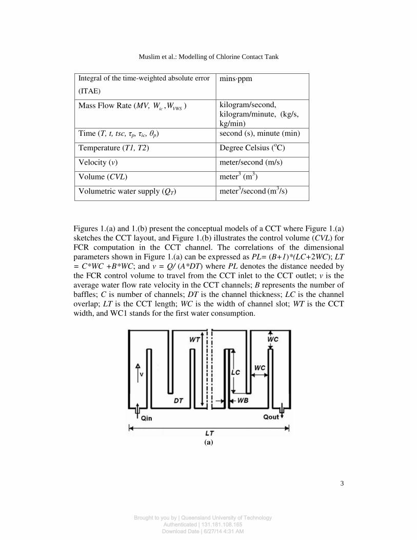
Figures 1.(a) and 1.(b) present the conceptual models of a CCT where Figure 1.(a)

sketches the CCT layout, and Figure 1.(b) illustrates the control volume (CVL) for

FCR computation in the CCT channel. The correlations of the dimensional

parameters shown in Figure 1.(a) can be expressed as PL= (B+1)*(LC+2WC); LT

= C*WC +B*WC; and v = Q/ (A*DT) where PL denotes the distance needed by

the FCR control volume to travel from the CCT inlet to the CCT outlet; v is the

average water flow rate velocity in the CCT channels; B represents the number of

baffles; C is number of channels; DT is the channel thickness; LC is the channel

overlap; LT is the CCT length; WC is the width of channel slot; WT is the CCT

width, and WC1 stands for the first water consumption.

(a)

3



(b)

Figure 1. a) the CCT layout, b) the FCR control volume (abbreviated as ‘FCR CVL’ in

the figure) in a CCT channel

A dynamic model of the FCR decay in the CCT can be developed from

both the CCT models shown in Figure 1, based on the overall mass balance for the

FCR in the CVL at the total residence time t (see Nauman, 2002, Seborg et al.,

2004). The CVL in the CCT is assumed to be constant, the FCR in the CVL

diminishes as the CVL travels along the CCT at the total residence time t. By

considering the CVL length (noted as the CCT length) from the point just after the

chlorine injection to a certain point along the CCT, the overall mass balance

equation can be rearranged as;

MCAcc = MC0F -MC - MCR (1)

where, MCAcc denotes the total FCR mass accumulation in the CVL over the total

residence time; MC0F is the total FCR mass in the inlet stream coming into the

CVL at the total residence time t; MC is the total FCR mass in the outlet stream

leaving the CVL at the total residence time t; and MCR indicates the total FCR

mass consumed due to chemical reactions in the CVL at the total residence time t.

Then, the overall mass balance for the FCR in the CVL at the total residence time t

is derived to be Equation (2):

( ) ( ) ( ) ( )oT T iT T oT CVL oT

dCVL X t Q X t Q X t kV X t

dt= − − (2)

where XiT is the initial FCR concentration in the CVL just after chlorine injection;

XoT is the FCR concentration in the CVL at the CCT outlet, which is known as the

controlled variable; k is the FCR rate constant; and QT is volumetric water supply

(VWS) in the CCT. Applying Laplace Transformation (Seborg et al., 2004), the

time domain solution of Equation (2) is obtained as:

4


DOI: 10.2202/1934-2659.1307


( )( ) 1 , ( ) /(1 )

niToT p p

r

XX t e n t

kθ τ

τ= − = − −

+ (3)

where the residence time, τr is predicted from PL/υ; the time constant, τp equals to

1/(PL/υ + k); θp is the time delay of the FCR decay process and can be also

calculated by θp = PL/υ. It can be observed that the FCR concentration, XoT = 0

when t = 0, and XoT = XiT/ (1 + τrk) when t → ~ (time approaches infinity), the

steady state gain (K) of the process is equal to 1/(1 + τrk), and the transfer function

of Equations (3) can be derived as:

( ) /(1 )s

T T pG s K e sθ τ−= + ,

1 1

1

iT

roTT

iT iT r

X

kXK

X X k

ττ

+∆ = = =

∆ + (4)

where GT (s) is the transfer function of the FCR decay process in the CCT, and KT

is the process gain.

The dynamic model for the mixing process of water flow and chlorine

injection (see Figure 1.b) can be derived from the steady state component balance

of ' ' ( )VWS w ic ic VWS ic iTW X W X W W X+ = + , and by applying Laplace Transformation of

the steady state model, the chlorine mixing process is described by:

'

( )1

ic iT

VWS icic

ic

X X

W WG s

sτ

−+

=+

, ( )1

VWS

VWS icVWS

VWS

W

W WG s

sτ+

=+

, Cic VWS

VWS ic

V

W W

ρτ τ= =

+ (5)

where Gic (s) is the transfer function of chlorine injection process; GVWS (s) is the

transfer function of the VWS just before chlorine injection; ic

W is the average mass

flow rate of pure component gaseous chlorine injected by the chlorine booster, as

the MV; VWS

W is the VWS mass flow rate before passing the boosters; 'wX is the

average FCR concentration in the VWS; τ is the process time constant; 'icX is the

average FCR concentration just after the injection of pure component gaseous

chlorine; and ρ is the density of solution after the mixing process.

The chlorine decay of stagnant flow denoted as SF, in the CCT needs to be

considered as the first disturbance in the system, symbolised as Gdv(s) shown in

Figure 2. The SF value can be obtained using the SF equation of

0 exp( )SF psc C ksc tsc= ⋅ − ⋅ , where C0 is the initial chlorine concentration; ksc is

the overall chlorine decay in the SF; psc is the portion of stagnant flow; and tsc is

the residence time for chlorine decay process in the SF.

5



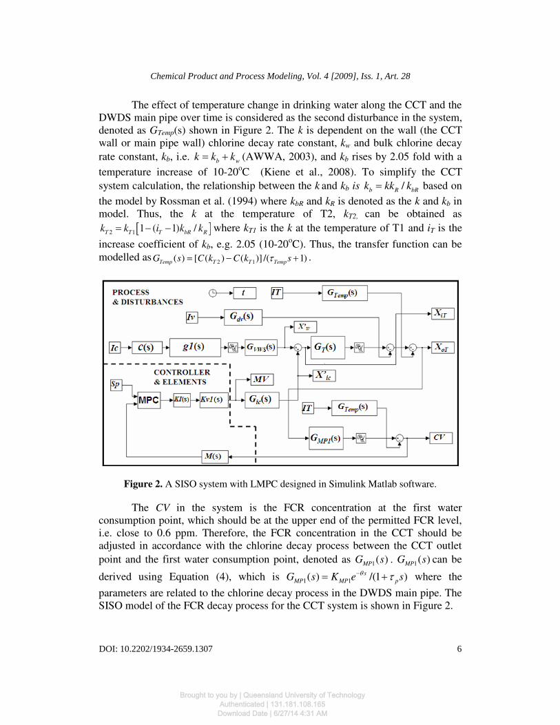
The effect of temperature change in drinking water along the CCT and the

DWDS main pipe over time is considered as the second disturbance in the system,

denoted as GTemp(s) shown in Figure 2. The k is dependent on the wall (the CCT

wall or main pipe wall) chlorine decay rate constant, kw and bulk chlorine decay

rate constant, kb, i.e. b w

k k k= + (AWWA, 2003), and kb rises by 2.05 fold with a

temperature increase of 10-20oC (Kiene et al., 2008). To simplify the CCT

system calculation, the relationship between the k and kb is /b R bR

k kk k= based on

the model by Rossman et al. (1994) where kbR and kR is denoted as the k and kb in

model. Thus, the k at the temperature of T2, kT2, can be obtained as

[ ]2 1 1 ( 1) /T T T bR Rk k i k k= − − where kT1 is the k at the temperature of T1 and iT is the

increase coefficient of kb, e.g. 2.05 (10-20oC). Thus, the transfer function can be

modelled as2 1( ) [ ( ) ( )] /( 1)Temp T T TempG s C k C k sτ= − + .

Figure 2. A SISO system with LMPC designed in Simulink Matlab software.

The CV in the system is the FCR concentration at the first water

consumption point, which should be at the upper end of the permitted FCR level,

i.e. close to 0.6 ppm. Therefore, the FCR concentration in the CCT should be

adjusted in accordance with the chlorine decay process between the CCT outlet

point and the first water consumption point, denoted as 1( )MP

G s . 1( )MP

G s can be

derived using Equation (4), which is 1 1( ) /(1 )s

MP MP pG s K e sθ τ−= + where the

parameters are related to the chlorine decay process in the DWDS main pipe. The

SISO model of the FCR decay process for the CCT system is shown in Figure 2.

6


DOI: 10.2202/1934-2659.1307


Linear Model Predictive Control

In this research, a model predictive control toolbox of Matlab is used to develop

the LMPC. With the functions given by the Matlab toolbox, LMPC can deal with

linear model presented in Simulink models (Bemporad et al., 2005). The LMPC

control objective is to regulate optimal mass flow rate of pure gaseous chlorine as

the MV of the CCT input order to control the FCR concentration at the first water

consumption at the required level based on GVWS(s), GT(s), Gic(s), GTemp(s) and

GMP1(s). In order to ensure the CV is regulated within the required range, the CV is

constrained within the range of 0.2-0.6 ppm. The control action can also be

computed subject to hard constraints on the MV and the CV: MVmin (i) ≤ MV(j +i)≤

MVmax (i); the MV rate constraints:|∆MV(j + i)| ≤ ∆MVmax (i); CVmin (i) ≤ CV(j +

l|j) ≤ CVmax (i) where i is the step input; j the step output; and k is the sampling

interval of prediction horizon.

The LMPC control performance is also dependent on the design

parameters that can be tuned, the model horizon, N (typically, 30 ≤ N ≤ 120),

moving horizon, M (typically, 5 ≤ M ≤ 20 and N/3 ≤ M ≤ N/2), prediction horizon,

P (P = N + M), output weight (OW), input weight (IW), rate weight (RW) and

control interval (CI) (Seborg et al., 2004).

Figure 2 shows the block diagram of LMPC designed using Matlab

Simulink to deal with the SISO system. Sp is the setpoint for the CV; KV1(s),

KI(s), and M(s) are the control elements of control valve, transducer, and

transmitter transfer function, respectively which are based on Seborg et al.,

(2004), the chlorine injection process (www.usfwt.com) and the assumptions

made. The simulation time is denoted as t (s); IT, Iv, and Ic are the inputs for

GTemp (s), and Gdv(s), respectively; c(s) is the value of VWSW based on the

equation of the steady state component balance; and g1(s) is the dynamic model

for the FCR fluctuation input to GVSW(s) when there is a fluctuation in the VWS.

Computational Fluid Dynamics

The purpose of using CFD in this study is to cross-check the regulation of the

optimal CV obtained by the LMPC in fluid dynamics simulation when actual fluid

flow is considered. In the model development of LMPC, the CCT tank geometry

is assumed to be a linear pipe line and it is informative to acquire the knowledge

of the fluid flow pattern in a baffled tank shown in Figure 1.(a) and the possible

consequence of the geometry on the FCR distribution.

In this research, the mixture multiphase model is used because it is

suitable for the chlorine mixing process of the CCT. The concept of phase volume

fraction is introduced. These volume fractions are assumed to be continuous

function of space and time (Fluent, 2003). To simplify the CFD simulation of the

CCT, 2D with steady-state condition solver is chosen, the SIMPLE (Semi-Implicit

7



Method for Pressure-Linked Equations) algorithm is a method for calculating

pressure and velocities as proposed by Versteeg and Malalasekera (1995). The

turbulence in this CCT phase has been modelled using a modified k-ε turbulence

model available in FLUENT 6.2, which was used in the turbulence model of

continuous flow reactor (Dennis et al., 2006).

In the first step of CFD simulation, GAMBIT 2.2 (pre-processor for

FLUENT 6.2) was used to create 2D geometries of the CCT with 4 m additional

main pipe at the CCT input and output as well as for its meshing. Small size

quadrilateral mesh was created for the area close to the distributor.

In the simulations, water (phase-1), chorine (phase-2) and ammonium

(phase-3) were taken as liquid, gas and liquid phase, respectively, with an

assumption that chlorine is instantly converted into FCR when dissolved in water.

The velocity inlet condition was applied at the distributor and the velocities as

well as volume fractions of both phases were specified appropriately. Based on

the data used in the LMPC simulation (a main pipe of 0.3048 m diameter

connected into the CCT input with the average VWS of 0.45 m3/s), the value of

X’W + X’ic (assumed as a volume fraction of 0.918 ppm) and the velocity inlet of

6.203 m/s as the boundary condition are applied with the operation condition of

pressure being 2068427 Pa (300 psig) based on the chorine capacity in the

available literature (Filter, 2003) at the inlet point [2.4 m, -4 m]. Mass transfer

rate of phase-2 into phase-3, 2.785E-5 /s, which is also used in the LMPC

simulation, is applied to present the CCT chlorine decay process.

RESULTS AND DISCUSSIONS

Matlab/Simulink Simulation

The simulated DWDS is assumed to have a main pipe of 0.3048 m diameter with

the average VWS of 0.45 m3/s which is 97.2% of Townsville water supply

(NQWater, 2006). The chlorine overall decay rate constant, k, is taken from

Rossman et al. (1994) related to the pipe diameter size of 0.3048 m, and the bulk

chlorine decay rate constant is taken as 0.55 mg/L per day. It is also assumed that

the first water consumption is located at 0.5 km from the chlorine booster with the

required FCR concentration of 0.6 ppm at which the chlorine disinfection of

Giardia cyst reaches 0.5-log reduction.

The CTcalc value is obtained as 0.806 ppm·minutes. The CTcalc/CT99.9

values are 0.0048, 0.0059 and 0.0039 for the plant with conventional filtration,

slow sand filter and membrane filtration value, respectively. The water

temperature is assumed to range from 5oC to 25

oC. Therefore, the simulated

DWDS needs a reservoir, i.e. CCT, after the chlorine booster for extra contact

time, prior to being distributed to the first consumer. The CCT domain description

8


DOI: 10.2202/1934-2659.1307


is B = 9 (C = 10), LC = 20.8 m, LT = 48.9 m, WC = 4.8 m, WT = 30.4 m and DT =

3 m (Government, 2006). With this CCT capacity, the CTcalc is obtained to be

approximately 162.1 minutes, which is 42.1 minutes longer than that the

maximum CT99.9 value required.

With regard to SISO system with the disturbances of GTemp(s) and Gdv(s),

and the LMPC elements, GVWS (s), Gic (s), GT(s) and GMP1(s) are obtained using

Equation (5) and the state component balance based on simulated data with the

assumption of X’W being 0.25 ppm. The VWS is assumed to be constant, being

0.45 m3/s because the velocity inlet/boundary condition for CFD simulation

should be constant, so that g1(s) is equal to 1. To obtain GTemp(s), the FCR

deviation is about 0.00220 ppm/ 0C based on a simulation with the bulk decay kb

being 2.1, the assumed ratio kb/k rises at a rate of 0.14 with a temperature change

from 50C to 25

0C per day with the repeating sequence input with time value of [0,

720] and output of [0, 20] used for the simulation. Gdv(s) is found through a CFD

study that the portion of stagnant flow being 1.5% in the CCT gives 0.1 ppm

changes in the FCR concentration at the CCT outlet. KI(s) I/P transducer

(Current-to-Pressure Transducer) is assumed to act as a linear device with

negligible dynamics (Seborg et al., 2004). The output signal from 3 to 300 psi

when input signal changes full-scale from 4 to 20 mA are assumed for the

feedback control, and these are normal scales in post-chlorination (Filter, 2003)

that yields KI(s) = 18.5625. To obtain KV1(s) = 90.909/ (0.0833s + 1), the zero and

span of each composition transmitter is assumed to be 0-6 ppm (the FCR mass

fraction, 0 – 6 x 10-6

kg FCR/ kg chlorine solution) with the output range assumed

to be 4-20 mA, and the time delay associated with measurement is assumed to be

0.5 minutes.

Figure 3 shows the FCR concentrations at various positions as a result of

PI controls and LMPC application over a period of 7 days. Because the dynamic

model is a fourth-order process, PI control with Ziegler-Nichols (ZN) tuning

setting; Kc = 20.83, τI = 0.105 (Seborg et al., 2004) is applied to get the better

performance. As can be seen in Figure 3.(a), in controlling the CV (the FCR

concentration at 0.55 km from the CCT outlet), the PI (ZN) control generated no

offset, and the CV settling time is about 3200 minutes. The decay ratio of the CV

is about 2/5, which is generally acceptable in terms of a controller performance

assessment (greater than 1/4). However, the CV at the time of approximately 960-

1320 minutes and 1680-2030 minutes is greater than the required upper level of

0.6 ppm, exceeding the upper limit of safe drinking water requirement. We can

also observe that the FCR concentration is still present until the point of 4.55 km

form the CCT outlet in the period between 245 and 705 minutes.

9



(a)

(b)

10


DOI: 10.2202/1934-2659.1307


(c)

Figure 3. The FCR concentration; (a) PI control (ZN tuning setting; Kc = 20.83, τI =

0.105), (b) PI control (ITAE method; Kc = 12.04, τI = 0.083), (c) LMPC (CI = 15, M =

30, P = 20, RW = 0.85, IW = 0.15, OW = 1).

The integral of the time multiplied by the absolute error (ITAE) was also

used to tune the PI control where the ITAE usually marks in the most conservative

controller setting (Seborg et al., 2004). As can be viewed in Figure 3.(b), the PI

(ITAE) control results in a more stable CV compared to the CV by PI (ZN)

control, and the settling time is approximately 890 minutes which is 570 minutes

faster than the one by PI (ZN) control. The maximum value of CV, 0.6612 ppm

(see the peak of the CV in Figure 3.b) is only slightly higher than the required

FCR upper level, which is 0.4588 ppm less than the overshoot (1.1200 ppm)

generated by PI (ZN) control (see the peak of the CV in Figure 3.(a)).

Compared to the PI (ZN) and PI (ITAE) control strategies, the LMPC

control performance appears superior. The CV controlled by the LMPC is much

more stable, the settling time is approximately 410 minutes which is 2790 minutes

faster than the one by PI (ZN) control, and 480 minutes faster than PI (ITAE).

Moreover, the fluctuation of FCR concentration is very small. The FCR

concentration is always within the required level of 0.2-0.6 ppm up to the point of

4.55 km from the CCT output (see the dot curve in Figure 3.a and Figure 3.b).

11



(a)

(b)

Figure 4. The LMPC performance (CI = 15, M = 30, P = 20, RW = 0.85, IW = 0.15, OW

= 1); (a) the mass flow rate of pure gaseous chlorine (MV), (b) the XiT and XoT profiles.

12


DOI: 10.2202/1934-2659.1307


In comparison, LMPC strategy provides the most stable control among the

3 methods. As justified by obtaining the CV ITAE values (Seborg et al., 2004), the

3 control strategies can be ranked as LMPC > PI (ITAE) control > PI (ZN)

control. Their CV’ ITAE values are approximately 1572, 1643, 2214 mins·ppm,

respectively. The disturbances of temperature and stagnant flow cause the

decrease in the FCR concentration at the CCT output which is approximately

1.0044 ppm less than the situation without the disturbances. This amount is

contributed by the 0.0044 ppm on the effect of increasing temperature and by the

0.1 ppm on the effect of stagnant flow based on the LMPC and PI simulations.

The stable responses of LMPC (see the solid line in Figure 4.a) is

attributed to one of the key features of LMPC in which we can put a constraint of

5.931E-6 to 1.067E-5 kg/minute at the LMPC output when designing the LMPC

to optimally adjust MV, a constraint of 0.2 to 0.6 ppm at the CV (see the solid line

in Figure 3.b). Therefore, if the upper constraint value of 1.067E-5 is multiplied

by both numerators of KIP(s) and KV(s), it yields the LMPC MV value of 0.018

kg/minute as shown in Figure 4.a. This LMPC MV value results in the FCR

concentration at the CCT input (XiT) and CCT output (XoT) of approximately 0.918

ppm and 0.638 ppm, respectively, as can be seen Figure 4.b. In contrast, we

cannot put any constraint in any PID control, so that the PI MV is oscillating as

can be seen by the dash line in Figure 4.a.

CFD Simulation

The CFD simulation results (steady-state profiles) are shown in Figure 5 when the

convergence occurred at the time of approximately 9000 s. As can be seen in

Figure 5.a, the CFD result is able to present the FCR decay and transport in the

CCT as the FCR travels along the CCT channel, the FCR concentration diminish

in proportion to its residence time from the CCT input to the CCT output. By

applying the FCR initial concentration of 0.918 (the LMPC XiT) obtained as the

optimal MV regulated by the LMPC, we are able to justify the SISO model

accuracy in presenting the FCR decay process and the LMPC performance which

is shown by the FCR concentration at the CCT outlet (the CFD XoT) as 0.618

ppm. The CFD XoT value of 0.618 ppm is reasonable because the disturbance of

temperature change of 0.0044 ppm cannot be included in the CFD simulation.

When the FCR concentration change of 0.0044 due to the disturbance is added

into the CFD XoT, the CFD XoT becomes 0.6224 ppm which is close to the LMPC

XoT of 0.638 ppm.

13



(a)

(b)

Figure 5. The CFD simulation results of the LMPC XiT; (a) contour of phase-2 (the

available FCR concentration along the CCT cannel) volume fraction, (b) contour of

phase-3 (the consumed FCR concentration by the organic compound along the CCT

cannel) volume fraction.

14


DOI: 10.2202/1934-2659.1307


Figure 5.b shows the mass transfer of phase-2 into phase-3 to represent the

FCR consumption by the organic compound in the CCT with the initial phase-3

volume fraction of 0.001 ppm. As can be seen in Figure 5.b, the phase-3 at the

CCT outlet is approximately 0.272 ppm. Compared to the reduced FCR

concentration being 0.28 ppm in the LMPC simulation, which is from 0.918 to

0.638 ppm, the CFD total mass change is consistent. The difference between the

LMPC results and the CFD results discussed above is approximately only 3.2 %.

The CFD simulation results confirm that the LMPC performance in controlling

the FCR in the CCT is very reasonable. Moreover, the CFD results indicate that

the fluid dynamics in such a baffled configuration of a CCT under the applied

flow rates has no noticeable effect on the FCR distribution. In real industrial

scenarios, the CFD simulations can be useful in control strategy design in

achieving the optimal control solution by taking the hydrodynamic distributed

parameters into account.

CONCLUSIONS

A SISO model has been developed in Matlab Simulink to present chlorine dosing

and chlorine decay processes in a CCT with considerations of the process

disturbances of temperature and stagnant flow in the CCT. To optimally control

FCR concentration in the SISO system, a LMPC has been designed. The LMPC

control objective is to regulate the optimal mass flow rates of gaseous chlorine to

control the FCR at water distribution points within the safe drinking water

requirements (0.2 – 0.6 ppm). A CFD model of chlorine transport and decay in the

CCT was also developed to cross-check the effects of initial chlorine

concentration, the disturbances, as well as the hydrodynamics.

The results on the LMPC and CFD simulations using a CCT in a simulated

DWDS, which has almost the same volumetry water supply (VWS) as the

reference real water plant, showed that the LMPC can control the FCR

concentration in the water distribution line within the constraints by regulating the

optimal mass flow rates of gaseous chlorine. The simulation results demonstrated

that the LMPC control strategy is superior to the conventional PI controls.

Moreover, the combination of CFD with control strategy simulations presents a

new direction in evaluating a control scheme particularly pertinent to fluid mixing

problems.

15



REFERENCES

American Water Works Association (AWWA), Treatment - Principles and

Practices of Water Supply Operation, 3rd ed. AWWA: Denver, Colorado,

USA, 2003, pp. 161-165.

Bellamy, W.D., Finch, G.R., and Haas, C. N., Integrated Disinfection Design Framework,

AWWA Research Foundation, Denver, CO., 1999.

Bemporad, A., Morari, M., and Ricker, N. L., Model Predictive Control Toolbox: For

Use with MATLAB, The MathWorks, Inc., Natick, 2005.

Brdys, M. A., Chang, T., and Duzinkiewicz, K., Intelligent Model Predictive Control of

Chlorine Residuals in Water Distribution Systems, Bridging the Gap: Meeting the

World’s Water and Environmental Resources Challenges (eds. Don Phelps and

Gerald Sehlke editor) Orland, Florida, May 20-24, 2001.

Chang, T., Brdys, M. A., and Duzinkiewi, K., Decentralized Robust Model

Predictive Control of Chlorine Residuals in Drinking Water Distribution

Systems, Proceedings of World Water and Environmental Resources

Congress, World Water and Environmental Resources Congress and

Related Symposia (eds. Paul Bizier and Paul DeBarry), Philadelphia,

Pennsylvania, June 23-26, 2003.

Dennis, J. G., Charles, N. H., and Bakhtier, F., “Computational Fluid Dynamic

Analysis of the Effect of Reactor Configuration on Disinfection Efficiency,”

Water Environment Research, vol. 78(9), 2006, pp. 909-919.

Dotson, D., and Heltz, G. R., Chlorine Decay Chemistry in Natural Waters, In

Water Chlorination: Environmental Impact and Health Effects (eds. R. L.

Jolley, W. A. Brungs and R. B. Cumming), Ann Arbor Science Publisher,

Inc., 1985, pp. 713-722.

Dougherty, D., and Cooper, D., A Practical Multiple Model Adaptive Strategy for

Single-Loop MPC, Control Engineering Practice, 2003, pp. 141-159.

Fluent, Fluent 6.1 User Guide, Lebanon, 2003.

Gas Chlorine Education Committee (GCEC), 2001. Available:

http://www.wwdmag.com/Gas-chlorine-Education -article 2620.

Government, O., Procedure for Disinfection of Drinking Water in Ontario: (As

adopted by reference by Ontario Regulation 170/03 under Safe Drinking

Water Act), Ontario, 2006. Available:

http://www.ontario.ca/drinkingwater/stel01_046942.pdf.

16


DOI: 10.2202/1934-2659.1307


Greene, D. J., Farouk, B., and Haas, C. N., “CFD Design Approach for Chlorine

Disinfection Processes”, Journal AWWA, vol. 96(8), August 2004, pp. 138-

150.

Hangos K. M., and Cameron I. T., Process Modelling and Model Analysis,

Academic Press, London, 2001.

Heraud, J., Kiene, L., Detay, M., and Levi, L., “Optimized Modeling of Chlorine

Residual in a Drinking Water Distribution System with a Combination of

On-line Sensors,” J. Water SRT-Aqua, vol. 46(2), 1997, pp. 59-70.

Imsland, L., Findeisen, R., Bullinger, E., Allgöwer, F., and Foss, B. A., “A Note

on Stability, Robustness and Performance of Output Feedback Nonlinear

Model Predictive Control,” Journal of Process Control, vol. 13, 2003, pp.

633-644.

Johnson, J. D., Measurement and Persistence of Chlorine Residual in Natural

Waters, Water chlorination: Environmental impact and health effects (ed. in

Jolle W R. L), Ann Arbor Science, Ann Arbor, Michigan, 1978, pp. 37-63.

Kiene, L., Lu, W., and Levi, Y., “Relative Important of the Phenomena

Responsible for Chlorine Decay in Drinking Water Distribution System,”

Wat. Sci. Tech., vol. 38 (6), 2008, pp. 219-227.

Liou, C.P., and Kroon, J.R., “Modeling the Propagation of Waterborne Substances

in Distribution Networks,” J. AWWA, vol. 79(11), 1978, pp. 54-58.

Mahmood, F., Pimblett, J., Grace, N., and Grayman, W., Evaluation of Mixing

Characteristics of Water Storage Tanks, Water Quality Technology

Conference, Seattle, WA USA, 10-14 Nov. 2002, pp. 2002.

MathWorks, Inc., MATLAB Release 7.0.1 Help Guidelines, 2005.

Muslim, A., Li, Q., and Tadé, M. O., Discrete Time-Space Model for Free

Chlorine Concentration Decay in Single Pipes of Drinking Water

Distribution System, Proceeding of Chemeca 2006 Conference in Auckland-

New Zealand (eds. B. R. Young, D. A. Patterson, and X. D. Chen), ISBN; 0-

86869-110-0, 18 September 2006, Paper No. 129/450.

Muslim, A., Li, Q., and Tadé, M. O., “Simulation of Free Chlorine Decay and

Adaptive Chlorine Dosing by Discrete Time-Space Model for Drinking

Water Distribution System,” Journal of Chemical Product and Process

Modelling, vol. 2(2), 2007, article 3.

Nauman, E.B., Chemical Reactor Design, Optimization, and Scaleup, New York,

McGraw-Hill, 2002.

17



NQWater, Townsville/Thuringowa Water Supply Upgrade Project, 2006.

Available: http://www.nqwater.com.au/?page=38.

Polycarpou, M. M, Uber, J. G., Wang, Z., Hang, F., and Brdys, M., “Feedback

Control of Water Quality, IEE Control System Magazine,” vol. 2, June 2002,

pp. 68-87.

Rossman, L. A., Clark, R. M., and Grayman, W. M., “Modelling chlorine residual

in drinking water distribution system,” J. Environmental Engineering, vol.

120(4), July/August 1994, pp. 803-820.

Rossman, L. A., EPANET2 Users Manual, EPA US: Cincinnati, USA, 2000.

Sakarya, B. A., and Mays, L. W., “Optimal Operation of Water Distribution

Pumps Considering Water Quality,” Journal of Water Resources Planning

and Management, August 2000, pp. 210-220.

Seborg, D. E., Edgar, T. F., and Mellichamp, D. A., Process Dynamic and

Control, USA, John Wiley & Son Inc., 2004.

Tarnawski, J., Brdys, M. A., and Duzinkiewicz, K., Supervised Model Reference

Adaptive Control of Chlorine Residuals in Water Distribution Systems,

Proceedings of World Water and Environmental Resources Congress and

Related Symposia (eds.Paul Bizier and Paul DeBarry), Philadelphia,

Pennsylvania, June 23-26, 2003.

Templeton, M. R., Hofmann, R., and Andrews, R. C., “Case Study Comparisons

of Computational Fluid Dynamics (CFD) Modeling Versus Tracer Testing

for Determining Clearwell Residence Times in Drinking Water Treatment”,

Journal of Environmental Engineering and Science, vol. 5(6), 1 November

2006, pp. 529-536.

U.S. Filter; S2K Sonic Chlorinator, 2003. Available:

http://www.wallaceandtiernan.usfilter.com.

Versteeg, H. K., and Malalasekera, W., An Introduction Fluid Dynamics: The

Finite Volume Method, Pearson Education Limited, England, 1995.

Wang, H., and Falconer, R. A., “Simulating Disinfection Processes in Chlorine

Contact Tanks Using Various Turbulence Models and High-Order Accurate

Difference Schemes”, Water Research, vol. 5, 1998, pp. 1529-1543.

Wang, Z., Polycarpou, M.M., and Uber, J.G., Decentralized Model References

Adaptive Control of Water Quality in Water Distribution Networks,

Proceedings of the 15th IEEE International Symposium on Intelligent

Control, Rio, Patras, Greece, July 2000, pp. 127-132.

18


DOI: 10.2202/1934-2659.1307


Wang, Z., Polycarpou, M M., Shang, F., and Uber, J. G., Design of Feedback

Control Algorithm for Chlorine Residual Maintenance in Water Distribution

Systems, Proceedings of World Water and Environmental Resources

Congress, Bridging the Gap: Meeting the World’s Water and Environmental

Resources Challenges (eds. Don Phelps and Gerald Sehlke), Orlando,

Florida, May 20-24, 2001.

Woolschlager, J., and Soucie, W. J., Chlorine Reactivity with Concrete Surfaces,

Proceedings of the World Water and Environmental Resource Congress,

World Water and Environmental Resource Congress and Related Symposia

(eds.P. Bizier and P. DeBarry), Philadelphia, Pennsylvania, USA, June 2003,

pp. 23-26.

19



chemical product and process modeling - griffith university

Documents