chemical modeling of iron (ii)/(iii) solutions in hydrometallurgy
TRANSCRIPT

CHEMICAL MODELING OF IRON(II)/(III) SOLUTIONS IN HYDROMETALLURGY USING OLI™
by
Michael Kardono Carlos
A thesis submitted in conformity with the requirements for the degree of Master of Applied Science
Department of Chemical Engineering and Applied Chemistry University of Toronto
© Copyright by Michael Kardono Carlos 2013

ii
CHEMICAL MODELING OF IRON(II)/(III) SOLUTIONS IN HYDROMETALLURGY USING OLI™
Michael Kardono Carlos
Master of Applied Science
Department of Chemical Engineering and Applied Chemistry
University of Toronto
2013
Abstract
Iron is the most common impurity in hydrometallurgy which is usually removed by precipitation
of insoluble iron compounds, such as hematite and jarosite. The knowledge of iron solubility in
multicomponent solutions is important for design and optimization of the iron removal steps.
The OLI Software package is a chemical modeling tool that incorporates the powerful mixed-
solvent electrolyte (MSE) model capable of performing simulations of multicomponent
electrolyte solutions from the freezing point up to the limit of fused salt and near the critical
temperature of the solution. Literature or experimental solubility data was fitted on the OLI
MSE model to improve the performance in simulating multicomponent Fe(II)/Fe(III) solutions.
The particular focus of this work aimed at developing simulation capability for the FeCl3-MgCl2-
HCl-H2O system through experimental solubility measurement and modeling, relevant to
atmospheric processing of saprolites by HCl using MgCl2 brines.

iii
Acknowledgments
Foremost, I would like to acknowledge my supervisor, Prof. Vladimiros G. Papangelakis for his
expertise, enthusiasm, patience, support and guidance over these three years which have made
me possible to finish my master study and achieve invaluable lessons which prepared me to step
into the real world.
I would also like to thank Prof. Charles Jia and Prof. Donald Kirk for spending their precious
time to sit down during my oral defense.
I would like to thank APEC group for their continuous support and creating great lab experience,
in particular, Igor Guzman, for offering his helping hand with my experimental setup; Ilya
Perederiy, Georgiana Moldoveanu, Douglass Duffy, and Anirudha Dani for their constructive
advice for my research. I also thank Srinath Garg, Steven Palmer, Wendy Zhou, Nazanin
Samadifard for their support.
I would like to thank George Kretschmann with the advice and lesson to conduct XRD analysis,
also to Dr. John Graydon for sharing his expertise with the TGA analysis.
I would like to thank Barrick Gold, Vale Canada Ltd., and OLI for their generous financial
support. I would also like to thank Dr. Peiming Wang for the technical support with performing
OLI regression.
I would like to acknowledge my families and friends for the continuous love and support which
has encouraged me to accomplish this milestone.

iv
Table of Contents
Acknowledgments .......................................................................................................................... iii
Table of Contents ........................................................................................................................... iv
List of Tables ............................................................................................................................... viii
List of Figures ................................................................................................................................ xi
Chapter 1 ......................................................................................................................................... 1
1 Introduction ................................................................................................................................ 1
1.1 Iron chemistry and its importance in hydrometallurgy ....................................................... 1
1.2 OLI Analyzer ...................................................................................................................... 4
Chapter 2 ......................................................................................................................................... 6
2 Literature Review and Theoretical Background ........................................................................ 6
2.1 OLI MSE Model ................................................................................................................. 6
2.1.1 Chemical Equilibrium ............................................................................................. 6
2.1.2 The HKFT Model ................................................................................................... 7
2.1.3 Activity Coefficient Model ..................................................................................... 7
2.2 Hydrometallurgical Treatment of Saprolite in Concentrated MgCl2 Brines ...................... 9
2.2.1 Current Technologies to Process Saprolite ............................................................. 9
2.2.2 More concentrated MgCl2 solutions ..................................................................... 10
2.3 Default OLI MSE's Performance in Modeling FeCl3 and MgCl2 Systems ...................... 14
2.3.1 Solubility of FeCl3 in water .................................................................................. 14
2.3.2 Solubility of FeCl3 in HCl solutions ..................................................................... 15
2.3.3 Solubility of Hematite in HCl solutions ................................................................ 15
2.3.4 Solubility of MgCl2 in Water ................................................................................ 16
2.3.5 Solubility of MgCl2 in HCl Solutions ................................................................... 17

v
2.3.6 Solubility of Hematite in MgCl2 and HCl Solutions ............................................ 18
2.4 Objectives ......................................................................................................................... 20
Chapter 3 ....................................................................................................................................... 22
3 Experimental ............................................................................................................................ 22
3.1 Experimental Setup ........................................................................................................... 22
3.2 Reagents ............................................................................................................................ 23
3.3 Experimental Procedures .................................................................................................. 24
3.3.1 FeCl3 Solubility in MgCl2 Solutions ..................................................................... 24
3.3.2 MgCl2 Solubility in FeCl3 Solutions ..................................................................... 24
3.3.3 Hematite Solubility in Acidic MgCl2 Solutions .................................................... 25
Chapter 4 ....................................................................................................................................... 26
4 Experimental Results and Discussion ...................................................................................... 26
4.1 Solubility of FeCl3 in MgCl2 Solutions ............................................................................ 26
4.1.1 Reproducibility Tests for FeCl3 Solubility in Water ............................................. 26
4.1.2 Kinetic Tests for FeCl3 Solubility in MgCl2 solutions.......................................... 26
4.1.3 FeCl3 Solubility Data in MgCl2 Solutions ............................................................ 28
4.2 Solubility of MgCl2 in FeCl3 Solutions ............................................................................ 32
4.2.1 Reproducibility Tests for MgCl2 Solubility in Water ........................................... 32
4.2.2 Kinetic Tests for MgCl2 Solubility in FeCl3 Solutions ......................................... 33
4.2.3 MgCl2 Solubility in FeCl3 Solutions ..................................................................... 34
4.3 Solubility of Hematite in MgCl2 and HCl Solutions ........................................................ 35
4.3.1 Reproducibility of Hematite Solubility in MgCl2 and HCl Solutions .................. 35
4.3.2 Kinetic Tests for Hematite Solubility in MgCl2 and HCl Solutions ..................... 37
4.3.3 Hematite Solubility Data in MgCl2 and HCl Solutions ........................................ 38
Chapter 5 ....................................................................................................................................... 40
5 OLI Modeling Results and Discussion .................................................................................... 40

vi
5.1 Fitting on the FeCl3-MgCl2-H2O System .......................................................................... 40
5.2 Maximum Achievable Solid Loading during Leaching .................................................... 44
5.3 Effect of FeCl3 Addition on MgCl2 Phase Diagram ......................................................... 47
5.4 Limitation of The OLI Model ........................................................................................... 48
5.5 OLI Model Improvement for Other Fe(II) and Fe(III) Systems ....................................... 51
Chapter 6 ....................................................................................................................................... 53
6 Conclusions .............................................................................................................................. 53
Chapter 7 ....................................................................................................................................... 56
7 Recommendation for Future Work .......................................................................................... 56
References ..................................................................................................................................... 57
Appendices .................................................................................................................................... 67
Appendix A: Determination of The Concentration of Fe(III), Mg and Free HCl ........................ 67
Appendix A-1: Determination of the concentration of Fe(III) ................................................. 67
Appendix A-2: Determination of the concentration of Mg ...................................................... 68
Appendix A-3: Free HCl determination ................................................................................... 70
Appendix B: Solubility Data of FeCl3, MgCl2 and Hematite in the Chloride Systems ................ 72
Appendix B-1: Solubility Data of FeCl3 in MgCl2 (and HCl) Solutions ................................. 72
Appendix B-2: Solubility Data of MgCl2 in FeCl3 Solutions .................................................. 78
Appendix B-3: Solubility Data of Hematite in MgCl2 and HCl Solutions .............................. 80
Appendix C: XRD Patterns of The Equilibrating Solid Phases .................................................... 88
Appendix C-1: XRD Patterns for FeCl3 Solubility Experiments ............................................. 88
Appendix C-2: XRD Patterns for MgCl2 Solubility Experiments ......................................... 102
Appendix C-3: XRD Patterns for Hematite Experiments ...................................................... 107
Appendix D: Analysis of the Double Salt 2.5FeCl3.MgCl2.7.5H2O ........................................... 109
Appendix E: Validation Plots and Model Improvement for Fe(II)/Fe(III) Systems .................. 113
Appendix E-1: FeSO4-H2O System ....................................................................................... 113

vii
Appendix E-2: FeSO4-H2SO4-H2O System ........................................................................... 114
Appendix E-3: FeSO4-MgSO4-H2O System .......................................................................... 117
Appendix E-4: FeSO4-MgSO4-H2SO4-H2O System .............................................................. 118
Appendix E-5: FeSO4-ZnSO4-H2SO4-H2O System ............................................................... 120
Appendix E-6: FeCl2-H2O System ......................................................................................... 122
Appendix E-7: FeCl2-HCl-H2O System ................................................................................. 123
Appendix E-8: FeCl2-MgCl2 System ..................................................................................... 125
Appendix E-9: FeCl2-MgCl2-HCl-H2O System ..................................................................... 126
Appendix E-10: Fe2O3-H2SO4-H2O System .......................................................................... 128
Appendix E-11: Fe2O3-MgSO4-H2SO4-H2O System ............................................................. 130
Appendix E-12: NaFe3(SO4)2(OH)6-H2SO4 System .............................................................. 132
Appendix F: Lists of Regressed OLI Parameters ....................................................................... 134

viii
List of Tables
Table 1: Regressed OLI parameters for FeCl3-MgCl2-H2O system ............................................. 40
Table 2: Comparison of the thermodynamic properties of the double salts ................................. 41
Table 3: Saprolite Ore Composition (Dry Basis) [6] .................................................................... 44
Table 4: Theoretical maximum dissolution of Fe, Ni, and Mg based on the solid loading .......... 45
Table 5: Summary of improved OLI model on Fe(II) and Fe(III) systems .................................. 51
Table A-1: The comparison between Fe(III) measurement from ICP and EDTA titration .......... 67
Table A-2: The comparison between Mg measurement from ICP and EDTA titration ............... 69
Table B-1: Solubility of FeCl3 in water from 25 up to 100°C ...................................................... 72
Table B-2: Kinetic data for FeCl3 solubility in water at 25°C ...................................................... 72
Table B-3: Kinetic data for FeCl3 solubility in 6 molal MgCl2 solutions at 25°C ....................... 73
Table B-4: Kinetic data for FeCl3 solubility in water at 40°C ...................................................... 74
Table B-5: Kinetic data for FeCl3 solubility in 1 molal MgCl2 solutions at 40°C ....................... 74
Table B-6: Kinetic data for FeCl3 solubility in 3 molal MgCl2 solutions at 40°C ....................... 75
Table B-7: Kinetic data for FeCl3 solubility in 5 molal MgCl2 solutions at 40°C ....................... 75
Table B-8: Solubility data of FeCl3 in MgCl2 solutions from 25 up to 100°C ............................. 75
Table B-9: Solubility data of FeCl3 in MgCl2 and HCl solutions from 25 up to 100°C ............... 77

ix
Table B-10: Solubility of MgCl2 in water from 25 up to 100°C .................................................. 78
Table B-11: Kinetic data for MgCl2 solubility in water at 25°C .................................................. 78
Table B-12: Kinetic data for MgCl2 solubility in 0.5 molal FeCl3 solutions at 25°C .................. 79
Table B-13: Solubility data of MgCl2 in FeCl3 solutions from 25 up to 100°C ........................... 79
Table B-14: Kinetic data for hematite solubility in 0.1 molal init. HCl at 60°C (measured) ....... 81
Table B-15: Kinetic data for hematite solubility in 0.1 molal init. HCl at 60°C (mass balance) . 81
Table B-16: Kinetic data for hematite solubility in 2.5 molal MgCl2 and 0.1 molal init. HCl at
60°C (measured) ........................................................................................................................... 82
Table B-17: Kinetic data for hematite solubility in 2.5 molal MgCl2 and 0.1 molal init. HCl at
60°C (mass balance) ..................................................................................................................... 82
Table B-18: Kinetic data for hematite solubility in 4 molal MgCl2 and 0.1 molal init. HCl at
60°C (measured) ........................................................................................................................... 83
Table B-19: Kinetic data for hematite solubility in 4 molal MgCl2 and 0.1 molal init. HCl at
60°C (mass balance) ..................................................................................................................... 83
Table B-20: Hematite Solubility in MgCl2 and HCl solutions at 60 and 90°C (measured) ......... 84
Table B-21: Hematite Solubility in MgCl2 and HCl solutions at 60 and 90°C (mass balance) ... 86
Table C-1: XRD peak lists for FeCl3 solubility in 1 molal init. MgCl2 solutions at 60°C ........... 94
Table C-2: XRD peak lists for FeCl3 solubility in 6 molal init. MgCl2 solutions at 60°C ........... 96
Table D-1: Double salt 2.5FeCl3.MgCl2.7.5H2O chemical analysis ........................................... 109

x
Table F-1: Default OLI MSE standard state parameters for solid and aqueous species ............. 134
Table F-2: Regressed standard state parameters of solid and aqueous species .......................... 134
Table F-3: Default OLI MSE mid-range binary interaction parameters between ions/aqueous
species ......................................................................................................................................... 135
Table F-4: Regressed mid-range binary interaction parameters between ions/aqueous species 136

xi
List of Figures
Figure 1: Variation of laterite profile with climate [4] ................................................................... 1
Figure 2: Simplified process flowsheet for saprolite processing with MgCl2 brines [6] .............. 10
Figure 3: MgCl2 phase diagram in H2O under MgO saturation [5] .............................................. 13
Figure 4: Default OLI MSE's simulated solubility of FeCl3 in water ........................................... 14
Figure 5: Default OLI MSE's simulated solubility of FeCl3 in HCl solutions.............................. 15
Figure 6: Default OLI MSE's simulated solubility of hematite in HCl solutions at 100°C .......... 16
Figure 7: Default OLI MSE's simulated solubility of MgCl2 in water ......................................... 17
Figure 8: Default OLI MSE's simulated solubility of MgCl2 in HCl solutions ............................ 18
Figure 9: Default OLI MSE's simulated solubility of hematite in MgCl2 solutions with constant
init. HCl at 60 and 90°C. The lines correspond to default OLI MSE's prediction results on the
solubility of hematite .................................................................................................................... 19
Figure 10: Default OLI MSE's simulated solubility of hematite in HCl solutions with constant
init. MgCl2 at 60 and 90°C. The lines correspond to default OLI MSE's prediction on hematite
solubility ....................................................................................................................................... 20
Figure 11: Experimental setup for low temperature solubility experiment .................................. 22
Figure 12: Experimental setup for high temperature solubility experiment ................................. 23
Figure 13: Reproducibility tests for the solubility of FeCl3 in water ............................................ 26
Figure 14: Kinetics for FeCl3 solubility in MgCl2 solutions at 25°C ........................................... 27
Figure 15: Kinetic tests for FeCl3 solubility in MgCl2 solutions at 40°C ..................................... 28
Figure 16: Solubility of FeCl3.6H2O in MgCl2 solutions at 25 and 35°C..................................... 29

xii
Figure 17: Solubility of 2.5FeCl3.MgCl2.7.5H2O in MgCl2 Solutions from 25 up to 100°C.
Symbols at 0 MgCl2 represent the solubility of FeCl3 hydrates in water. .................................... 30
Figure 18: XRD Spectra of the double salt from 3 molal init. MgCl2 experiment at 60°C .......... 32
Figure 19: Reproducibility tests for the solubility of MgCl2 in Water ......................................... 33
Figure 20: Kinetic Tests for Solubility of MgCl2 in FeCl3 Solutions ........................................... 34
Figure 21: Solubility of MgCl2 in FeCl3 Solutions from 25 up to 100°C ..................................... 35
Figure 22: Reproducibility issues in the solubility of hematite in MgCl2 and HCl solutions ...... 36
Figure 23: Vapor-Liquid Equilibria of HCl in MgCl2 Solutions .................................................. 36
Figure 24: Kinetic tests for hematite solubility in 0.1 molal HCl initially and varying MgCl2
concentration ................................................................................................................................. 38
Figure 25: Solubility of hematite in MgCl2 and HCl solutions at 60 and 90°C ........................... 39
Figure 26: OLI fitting on the solubility of FeCl3.6H2O in MgCl2 solutions ................................. 42
Figure 27: OLI fitting on the solubility of 2.5FeCl3.MgCl2.7.5H2O in MgCl2 solution. The
dashed lines represent the solubility of FeCl3 hydrates at low MgCl2 concentration. .................. 42
Figure 28: OLI fitting on the solubility of MgCl2 in FeCl3 solutions ........................................... 43
Figure 29: OLI prediction on the solubility of FeCl3 in MgCl2 and HCl solutions ...................... 43
Figure 30: Maximum solid loading achievable based on OLI Prediction .................................... 45
Figure 31: OLI's Predicted MgCl2-FeCl3-H2O ternary phase diagram ......................................... 48
Figure 32: Predicted solubility of hematite in HCl solutions ....................................................... 49
Figure 33: Predicted solubility of hematite in MgCl2 and HCl solutions ..................................... 50
Figure 34: Predicted hematite solubility in MgCl2 solutions at const. free HCl ........................... 51

xiii
Figure C-1: XRD pattern for FeCl3 solubility in water at 25°C ................................................... 88
Figure C-2: XRD pattern for Solubility of FeCl3 in 6 molal init. MgCl2 solutions at 25°C ......... 89
Figure C-3: XRD pattern for FeCl3 solubility in water at 35°C ................................................... 90
Figure C-4: XRD pattern for FeCl3 solubility in water at 40°C ................................................... 91
Figure C-5: XRD pattern for FeCl3 solubility in 1 molal init. MgCl2 solutions at 40°C .............. 92
Figure C-6: XRD pattern for FeCl3 solubility in 3 molal init. MgCl2 solutions at 40°C .............. 93
Figure C-7: XRD pattern for FeCl3 solubility in 1 molal init. MgCl2 solutions at 60°C .............. 94
Figure C-8: XRD pattern for FeCl3 solubility in 6 molal init. MgCl2 solutions at 60°C .............. 96
Figure C-9: XRD pattern for FeCl3 solubility in 1 molal init. MgCl2 solutions at 80°C .............. 98
Figure C-10: XRD pattern for FeCl3 solubility in 3 molal init. MgCl2 solutions at 80°C ............ 99
Figure C-11: XRD pattern for FeCl3 solubility in 1 molal init. MgCl2 at 100°C ....................... 100
Figure C-12: XRD pattern for FeCl3 solubility in 3 molal init. MgCl2 solutions at 100°C ........ 101
Figure C-13: XRD pattern for MgCl2 solubility in 1.5 molal init. FeCl3 solutions at 25°C ....... 102
Figure C-14: XRD pattern for MgCl2 solubility in 0.5 molal FeCl3 solutions at 80°C .............. 103
Figure C-15: XRD pattern for MgCl2 solubility in 2 molal init. FeCl3 solutions at 80°C .......... 104
Figure C-16: XRD pattern for MgCl2 solubility in 0.5 molal FeCl3 solutions at 100°C ............ 105
Figure C-17: XRD pattern for MgCl2 solubility in 1 molal FeCl3 solutions at 100°C ............... 106
Figure C-18: XRD pattern for hematite solubility in 0.1 molal HCl and 2.5 molal MgCl2 at 60°C
..................................................................................................................................................... 107
Figure C-19: XRD pattern for hematite solubility in 0.1 molal HCl, sat'd MgCl2 solutions at 60°C
..................................................................................................................................................... 108

xiv
Figure D-1: First TGA analysis of the double salt 2.5FeCl3.MgCl2.7.5H2O .............................. 111
Figure D-2: Second TGA analysis of the double salt 2.5FeCl3.MgCl2.7.5H2O ......................... 112
Figure E-1: Default OLI MSE's simulated solubility of FeSO4 in water .................................... 113
Figure E-2: Improved OLI MSE's simulated FeSO4 solubility in water .................................... 114
Figure E-3: Default OLI MSE's simulated FeSO4 solubility in H2SO4 solutions up to 100°C .. 115
Figure E-4: Improved OLI MSE's simulated FeSO4 solubility in H2SO4 solutions up to 100°C 115
Figure E-5: Default OLI MSE`s simulated FeSO4 solubility in H2SO4 solutions above 100°C 116
Figure E-6: Improved OLI MSE`s simulated FeSO4 solubility in H2SO4 solutions above 100°C
..................................................................................................................................................... 116
Figure E-7: Default OLI MSE's simulated FeSO4 solubility in MgSO4 solutions ..................... 117
Figure E-8: Improved OLI MSE's simulated FeSO4 solubility in MgSO4 solutions .................. 118
Figure E-9: Default OLI MSE's simulated FeSO4 solubility in MgSO4 and H2SO4 solutions ... 119
Figure E-10: Improved OLI MSE's simulated FeSO4 solubility in MgSO4 and H2SO4 solutions
..................................................................................................................................................... 119
Figure E-11: Default OLI MSE's simulated FeSO4 solubility in ZnSO4 and H2SO4 solutions .. 120
Figure E-12: Improved OLI MSE's simulated FeSO4 solubility in ZnSO4 and H2SO4 solutions121
Figure E-13: Default OLI MSE's simulated FeSO4 solubility in ZnSO4 and H2SO4 solutions at
200°C .......................................................................................................................................... 121
Figure E-14: Improved OLI MSE's simulated FeSO4 solubility in ZnSO4 and H2SO4 solutions at
200°C .......................................................................................................................................... 122

xv
Figure E-15: Default OLI MSE's simulated FeCl2 solubility in water ....................................... 123
Figure E-16: Default OLI MSE's simulated FeCl2 solubility in HCl solutions .......................... 124
Figure E-17: Improved OLI MSE's simulated FeCl2 solubility in HCl solutions....................... 124
Figure E-18: Default OLI MSE's simulated FeCl2 solubility in MgCl2 solutions ...................... 125
Figure E-19: Improved OLI MSE's simulated FeCl2 solubility in MgCl2 solutions ................... 126
Figure E-20: Default OLI MSE's simulated FeCl2 solubility in MgCl2 and HCl solutions ........ 127
Figure E-21: Improved OLI MSE's simulated FeCl2 solubility in MgCl2 and HCl solutions .... 127
Figure E-22: Default OLI MSE's simulated Fe2O3 solubility in H2SO4 solutions at 130-170°C 128
Figure E-23: Improved OLI MSE's simulated Fe2O3 solubility in H2SO4 solutions at 130-170°C
..................................................................................................................................................... 129
Figure E-24: Default OLI MSE's simulated Fe2O3 solubility in H2SO4 solutions at 230-270°C 129
Figure E-25: Improved OLI MSE's simulated Fe2O3 solubility in H2SO4 solutions at 230-270°C
..................................................................................................................................................... 130
Figure E-26: Default OLI MSE's simulated Fe2O3 solubility in MgSO4 and H2SO4 solutions .. 131
Figure E-27: Improved OLI MSE's simulated Fe2O3 solubility in MgSO4 and H2SO4 solutions
..................................................................................................................................................... 131
Figure E-28: Default OLI MSE's simulated Na-jarosite solubility in H2SO4 solutions ............. 132
Figure E-29: Improved OLI MSE's simulated Na-jarosite solubility in H2SO4 solutions .......... 133

1
Chapter 1
1 Introduction
1.1 Iron chemistry and its importance in hydrometallurgy
Iron is considered as a major impurity in hydrometallurgical processing circuits due to its
mineralogical abundance. At a certain point of the process, and in order to obtain purified pay
metal products, iron needs to be separated most often by precipitation of various iron
compounds, such as hematite (Fe2O3), goethite (FeOOH) or jarosite (XFe3(SO4)2(OH)6, where X
is usually a monovalent cation, e.g. H3O+, NH4
+, Na
+, K
+, Ag
+, 1/2Pb
2+). Hematite is the most
desired iron compound since it is thermodynamically stable, has high Fe content per unit mass,
and is commercially saleable if pure [1]. On the other hand, jarosite precipitation allows sulfate
and alkali metal removal but it has low Fe content per unit mass and it is unstable under certain
storage conditions [2, 3]. For example, in processing nickel from lateritic ores, the
hydrometallurgical treatment varies depending on the types of laterites, whether it is limonitic
laterite or saprolitic laterite. Figure 1 shows the distribution of lateritic ores with depth and
climate.
Figure 1: Variation of laterite profile with climate [4]

2
Limonitic laterites are oxide ores, which are rich in iron and low in magnesium content and are
commonly processed by using pressure acid leach with sulfuric acid. Iron which mainly exists as
goethite in the ore is dissolved by acid attack and precipitated in-situ as hematite, which
regenerates the stoichiometric equivalent of acid as per reactions given below.
2FeOOH (s) + 3H2SO4 (aq) → Fe2(SO4)3 (aq) + 4H2O (l) (1-1)
Fe2(SO4)3 (aq) + 3H2O (l) → Fe2O3 (s) + 3H2SO4 (aq) (1-2)
As a result, acid is only required to bring the value metals (i.e. Ni and Co) into the solution, as
well as the minor impurities, e.g. Ca, and Al. The presence of monovalent cations in the leach
solution promotes jarosite precipitation instead of hematite. While this process is efficient in
processing limonitic laterites, it suffers from high acid consumption when processing saprolitic
laterites. The reason is that saprolitic laterites are rich in Mg, which will be dissolved by acid
attack, thus greatly increasing the acid requirements. This is partially due to the sulfate-bisulfate
equilibrium, i.e. sulfate addition shifts the equilibrium towards bisulfate formation, thus
decreasing the available protons for leaching.
Alternatively, this type of ore can be treated by chloride hydrometallurgy, in particular in the
presence of MgCl2 brines [5]. This process, which is mainly targeted to limit the Mg dissolution,
also improves the acid activity and allows the recovery of dry HCl(g). Furthermore, the use of
chloride brines would elevate the boiling point of the solutions, thus making it possible to run the
process at temperatures higher than 100°C while maintaining atmospheric pressure, which
simplifies the types of equipment used without the need to use pressurized vessels. Moreover,
chloride salts are generally extremely soluble, which could be utilized to minimize the size of the
equipment, thus reducing the capital costs of running the process.
An HCl/MgCl2 solution used as lixiviant will dissolve the oxides in the ore to metal chlorides.
Recent study indicates that Ni and Co dissolution follows Fe dissolution from the oxide phase [6]
and since chloride ion strongly forms complexes with Fe(III), in-situ hematite precipitation is
hindered. Therefore, the idea behind chloride hydrometallurgy is to dissolve all of the Fe to
completely release the Ni and Co to the solution. In this case, the leaching process is not focused

3
on minimizing acid consumption, as compared to the sulfate hydrometallurgy, but to regenerate
all of the chloride units consumed (from HCl) as HCl(g). Based on these findings, the
knowledge of the solubility of Fe(III) under this condition would be beneficial to evaluate the
maximum solid to liquid ratio (solid loading) that can be processed during the leaching step
without losing the chloride units from precipitation of metal chlorides, in this case FeCl3. The
dissolved Fe(III) content is removed as hematite during the neutralization stage by MgO addition
which further increases the MgCl2 concentration in the solution. The knowledge of the solubility
of hematite under concentrated MgCl2 solutions can be utilized to monitor the efficiency of the
iron removal during this process. A detailed description of this process will be discussed in the
next chapter.
Other examples, such as the Akita Zinc Hematite Process, involves neutral leaching of residue in
the form of zinc ferrite (ZnFe2O4) to remove iron as hematite and recover valuable metals (e.g.
Cu, Ga and In) [7, 8]. First, the residue is leached in hot spent H2SO4 solutions, with the addition
of SO2 to reduce Fe(III) to Fe(II) as follows [7]:
ZnFe2O4 (s) + SO2 (l) + 2H2SO4 (aq) → ZnSO4 (aq) + 2FeSO4 (aq) + 2H2O (l) (1-3)
Following neutralization takes place using limestone (CaCO3) to remove valuable metals and
certain impurities from the solution. This reduction of iron allows it to remain in the solution
without undergoing hydrolysis at pH up to 4 [7]. The solution is then subjected to oxidation-
hydrolysis, namely oxydrolysis, inside an autoclave at 200°C, at O2 overpressure of 100-500
kPa, which regenerates H2SO4 and produces hematite as seen in Eq. 1-4 [7, 8].
2FeSO4 (aq) + 0.5O2 (g) + 2H2O (l) → Fe2O3 (s) + 2H2SO4 (aq) (1-4)
However, the solubility of FeSO4 decreases with increasing temperature above 55°C, even more
drastic at temperatures above 100°C [9, 10, 11], thus the knowledge of solubility of FeSO4 in the
presence of acidic ZnSO4 solutions at elevated temperatures is beneficial in avoiding the
potential precipitation of FeSO4.H2O prior to/during oxydrolysis [12]. For the case of steel
pickling process using HCl to remove the FeO scale [13], as well as the non-oxidative/oxidative
chloride leaching process for sulfide minerals using FeCl2+HCl [14] and FeCl3+HCl [15],
respectively, it is important to understand the solubility of FeCl2 in multicomponent HCl
4
solutions at elevated temperatures for figuring out the maximum holding of Fe(II) in that system
to prevent chloride loss for HCl regeneration.
In order to control and optimize such iron removal processes requires the knowledge of the
solubility of iron (II) and (III) in the multicomponent solutions of interest. Development of such
data takes significant amount of experimental work. However, the use of reliable chemical
models can save the industry a considerable amount of time and money.
1.2 OLI Analyzer
The OLI analyzer software package, which was developed by OLI Systems Inc., is capable of
performing simulations of electrolyte solutions at equilibrium. The software features
simultaneous calculation of phase and speciation equilibria along with thermal and volumetric
properties of the mixture. It runs under two main thermodynamic frameworks, either the older
aqueous (AQ) model or the new mixed-solvent electrolyte (MSE) model. The limits of the MSE
model range from below the freezing point to 90% Tcrit of the solution, from 0 to 1500 bar, and
no limit for the ionic strength [16]. The new MSE model works for systems from infinite
dilutions up to the fused salt limit, as well as systems involving mixed-solvent system of organic-
water [16]. For accurate simulations of hydrometallurgical processing solutions, which are
concentrated and possess high degree of non-ideality, the MSE model was selected as the
framework in this study. In addition, model customization was achieved by utilizing the built-in
regression facility with the purpose of either adding new chemical systems or improving the
performance of the current commercial OLI database.
The breakdown of the chapters in this thesis is as follows:
Chapter 2 discusses the fundamentals behind the OLI MSE model, the chemistry behind
the hydrometallurgical treatment of saprolites using MgCl2 brine, and the project
objectives.
Chapter 3 focuses on the experimental methodology used to perform the solubility study.
This chapter includes the experimental setup, the reagents used and the experimental
procedures.

5
Chapter 4 discusses the experimental results for the solubility of FeCl3 in MgCl2, the
solubility of MgCl2 in FeCl3 and the solubility of hematite in MgCl2 and HCl solutions.
Chapter 5 discusses the OLI MSE model improvement through regression of the new
solubility data of FeCl3, MgCl2, and Fe2O3 in chloride systems, and attempts some
extensions relevant to hydrometallurgical applications.
Chapter 6 and Chapter 7 discuss the conclusion of this work and the recommendation
for future work, respectively.

6
Chapter 2
2 Literature Review and Theoretical Background
2.1 OLI MSE Model
2.1.1 Chemical Equilibrium
The equilibrium expression for the general chemical reaction:
aA + bB + … = cC + dD + … (2-1)
is expressed as:
(
) (2-2)
Where R is the ideal gas constant, T is the temperature, xi is the mol fraction of species i, and γi is
the activity coefficient of species i. Meanwhile, the standard-state Gibbs free energy of the
reaction ΔG°, is given by:
∑
(2-3)
which summates all the standard-state chemical potential μi0 of the species i, participating in the
reaction shown in Eq. 2-1 and multiplied by its stoichiometric coefficient, vi with the value
being positive and negative for the species on the product side and reactant side, respectively. In
order to calculate the standard-state chemical potential of the solid species, basic thermodynamic
relationships are used to derive the following equation [17]:
( ) ∫ ∫ (
)
∫
(2-4)
where Δ and
are respectively, the standard partial molal Gibbs free energy of formation
and standard partial molal entropy of the species at 298.15K and 1 bar. P and T correspond to
the pressure and temperature of the system, respectively, while those with the subscript "r"
correspond to the reference conditions which are 298.15K and 1 bar.

7
For aqueous neutral or ionic species, the model needs to predict standard-state properties up to
high temperatures and pressures. In OLI MSE, this is achieved by employing the Helgeson-
Kirkham-Flower-Tanger (HKFT) equation of state. Furthermore, solving for the mole fractions
in Eq. 2-2 it is understood that the activity coefficients are also functions of the mole fractions.
2.1.2 The HKFT Model
The revised HKFT equation of state was developed by Helgeson and co-workers to estimate the
standard state thermodynamic properties of aqueous species [18, 19, 20] at elevated temperatures
and pressures. The expression of the standard partial molal Gibbs Free energy of formation of
any aqueous species ΔG0
P,T is as follows:
( ) ( ) (
)
[ ( ) (
)] (
) [ (
) ]
[{(
) (
)} (
)
(
( )
( ))] (
)
(
) ( ) (2-5)
The species dependant HKFT parameters are a1, a2, a3, a4, c1, c2, and ω. Ψ and θ are the
solvent dependent parameters having the values of 2600 bar and 228K for water, respectively. ε
is the dielectric constant of water and the Born Function,
(
)
while the value of
= -5.8x10⁻⁵ K-1
. The database for the HKFT parameters for various aqueous organic and
inorganic species is available in the series of papers published by Helgeson, Shock, and
coworkers [21, 22, 23, 24, 25] or they can be estimated through regression.
2.1.3 Activity Coefficient Model
The activity coefficient is the parameter that describes the degree of non-ideality of the solution.
It is computed based on the excess Gibbs free energy of the solution, Gex
, as follows:

8
( (
)
)
(2-6)
The activity coefficient model incorporated in OLI MSE takes into account the full concentration
range, from a dilute solution which is dominated by long range electrostatic forces, to
concentrated solutions up to the fused salt limit, which is governed by the mid-range ion-ion/ion-
molecule interactions and the short range ion-ion/ion-molecule/molecule-molecule interactions.
As seen in Eq. 2-7, the total excess Gibbs free energy is defined as the sum of the contributions
from all the three ranges [16].
(2-7)
The long-range interaction is described by Pitzer-Debye Hückel expression [26, 27] due to its
effectiveness in reproducing experimental in electrolyte solutions [28, 29, 30, 31], as well as
mixed-solvent electrolyte system [28, 32, 33]. On the other hand, the short-range contributions
are more relevant to mixed-solvent electrolyte solutions which are modeled by using the
UNIQUAC model. The expressions for the long and short-range interactions are available in the
original paper [16]. The concentrated electrolyte solutions of interests to hydrometallurgical
applications are dominated by ionic strength dependent mid-range interactions having the form
of second virial coefficient-type of expression as follows:
(∑ )∑ ∑ ( ) (2-8)
where Bij(Ix) represents the binary interaction parameter between two charged species or a
charged species with neutral molecule with Bij(Ix)=Bji(Ix) and Bii=Bjj=0. The functionality of the
Bij(Ix) is shown in Eqs. 2-9 to 2-11 with b(0-2)ij and c(0-2)ij as the adjustable temperature
independent parameters which are proven to be effective in reproducing experimental data [34].
( ) ( √ ) (2-9)
bij= b0,ij+ b1,ijT + b2,ij/ T (2-10)
cij= c0,ij+ c1,ijT +c2,ij/ T (2-11)

9
2.2 Hydrometallurgical Treatment of Saprolite in Concentrated MgCl2 Brines
2.2.1 Current Technologies to Process Saprolite
A pyrometallurgical process, rotary-kiln electric furnace (RKEF) has been commercially used to
treat saprolite [35]. This process starts with ore-drying inside a rotary kiln at 100°C which
removes the moisture content of the ore. The dried ore moves to another rotary kiln at 700-
900°C which removes the crystalline water by calcination. In this step, coke is generally added
to reduce the nickel and iron oxide back to the metallic state to form ferronickel which is
separated from the iron oxide and silicate slag inside an electric furnace at 1600°C. While the
nickel recovery is above 90% and it can handle high magnesium content, this process requires
high capital cost, and is highly energy intensive [36]. Attempts have been made to process this
type of ore using hydrometallurgy. The high acid requirement due to Mg dissolution and the
unavailability to recover the acid used to dissolve Mg has rendered saprolite not feasible to be
treated using HPAL.
Alternatively, chloride hydrometallurgy to process saprolites has been attempted by Intec [37],
Jaguar [38, 39] and Anglo Base [40] due to the following benefits: high solubility of most metal
chlorides, aggressiveness of HCl to leach the silicate ores even at atmospheric conditions,
minimized scale formation because no calcium sulfate or alunite forms, and the potential to
regenerate HCl. More so, high concentration of chloride increases the activity of the hydrogen
ion [41, 39, 42, 43] (which results in a more efficient leaching using close to stoichiometric HCl
requirements) as well as increase of the solution boiling point to above 100°C which improves
leaching kinetics while maintaining atmospheric conditions. The use of concentrated MgCl2 as
the lixiviant would serve for this purpose as well as limit the dissolution of Mg from the ores
[44]. However, none of the process to treat saprolite has been commercialized, mainly due to
issues with the recovery of HCl. Solution pyrohydrolysis is a conventional method to recover up
to azeotropic HCl (20%), as conceptually implemented by Jaguar Nickel [39, 45] and performed
by the steel pickling industry [46, 47, 48, 49], but it suffers from high energy requirement from
boiling off the excess water and water balance issues of the recycled HCl solutions. In this
process, the MgCl2 brine which is fed to a fluidized bed/spray roaster is contacted with hot
combustion gas at 560-700°C and underwent a hydrolysis reaction to produce MgO and HCl.
Much research attention has been focused towards hydrolytic distillation of HCl which mainly

10
involves hydrolysis of the ferric chlorides at atmospheric pressure and temperatures below
200°C to form superazeotropic HCl (8-9M) and hematite [42, 50, 51, 52]. This process was first
implemented in the 1970s by PORI Inc. In the PORI process HCl is regenerated from the spent
steel pickling liquor by oxydrolysis of a FeCl2 solution [53, 54, 55, 56]. Even though higher
grade of HCl can be achieved as compared to that of pyrohydrolysis, the pre-evaporation step to
concentrate the FeCl2 brine and the use of autoclave during oxidation to FeCl3 rendered this
process economically unattractive. A recent modification by McGill University allows HCl
regeneration from MgCl2-FeCl3 brines but the precipitation of MgCl2.xH2O as well as the MgCl2
hydrolysis product, Mg(OH)Cl.xH2O at 200°C hinders the hydrolysis step [51].
2.2.2 More concentrated MgCl2 solutions
A process idea was recently developed in our group, uses concentrated MgCl2 and HCl as the
lixiviants, and is capable of treating saprolite ore as well as recover dry HCl gas by employing
precipitation, dehydration, and decomposition of magnesium hydroxychloride [5].
Figure 2: Simplified process flowsheet for saprolite processing with MgCl2 brines [6]
First, saprolite ore is subjected to leaching with HCl in MgCl2 brine, where most of the metal
contents of the ore are dissolved to form a metal chloride solution (with minimal dissolution of
magnesium due to common ion effect) while the remaining unleached residue is disposed. The
dissolved iron fraction is removed using MgO as either anhydrous or hydrated iron oxide or iron
oxyhydroxychloride (akageneite). The leaching and the iron control steps will be discussed
further in the next sections. Further MgO addition precipitates base metals as hydroxides. The
remaining MgCl2 brine is precipitated as the double salt, magnesium hydroxychloride by excess
MgO based on the following reactions [5]:

11
2MgO (s) + MgCl2 (aq) + 6H2O (aq) 2MgO.MgCl2.6H2O (s) (2-11)
3MgO (s) + MgCl2 (aq) + 11H2O (aq) 3MgO.MgCl2.11H2O (s) (2-12)
The double salts, 2MgO.MgCl2.6H2O and 3MgO.MgCl2.11H2O are referred as “2-form” and “3-
form”, respectively. While the “2-form” forms at temperature above 90°C and 35 wt% MgCl2,
the “3-form” requires temperature as low as 80°C and 30 wt% MgCl2. This way, the chloride
units are locked into the solid phase, which then is subjected to dehydration to remove the
moisture and crystalline water contents at 230°C and 180°C for the “2-form” and “3-form”,
respectively, as follows [5]:
2MgO.MgCl2.6H2O (s) 2MgO.MgCl2.H2O (s) + 5H2O (g) (2-13)
3MgO.MgCl2.11H2O (s) MgO (s) + 2MgO.MgCl2.H2O (s) + 10H2O (g) (2-14)
The final step is the decomposition of the magnesium hydroxychloride at 560°C to produce dry
HCl gas for recycling and saleable/recycleable MgO product [5].
2MgO.MgCl2.H2O (s) 3MgO (s) + 2HCl (g) (2-15)
The advantages of this process are:
1. Only the water that remains in the magnesium hydroxychloride solid phase needs to be
evaporated in the dehydration step, thus minimizing the energy usage as compared to
solution pyrohydrolysis. The energy required for “2-form” and “3-form” are 10.7
GJ/tonne HCl and 15.9 GJ/tonne HCl, respectively, as compared to 15 wt% and 25 wt%
MgCl2 solution pyrohydrolysis which require 16.5 GJ/tonne HCl and 28.6 GJ/tonne HCl,
respectively [5].
2. The temperature of the decomposition step (560°C) is much lower than that of solution
pyrohydrolysis (700-900°C)
3. The production of anhydrous HCl (g) eliminates water balance issues and produces
water-free HCl.

12
2.2.2.1 Leaching Step
During chloride leaching of saprolite, the following general reaction occurs:
(Fex, Niy, Mg(2-1.5x-y))SiO4 (s) + 4HCl (aq) xFeCl3 (aq) + yNiCl2 (aq) + (2-1.5x-y)MgCl2 (aq)
+ SiO2 (s) + 2H2O (l) (2-16)
The leach solutions consist primarily of FeCl3, MgCl2, NiCl2 and free HCl and leaving behind
unleached magnesium silicate and silica. Leaching tests were studied at MgCl2 concentration of
2 and 4.5 molal, temperature of 100°C and solids loading of 10, 15, and 25% [6]. The
hydrolysis of iron is inhibited due to the high chloride content of the solution, which leads to the
formation of ferric chloride complexes, thus shifting the equilibrium from Fe2O3 towards
FeCl3(s). The question arises at what is the maximum solid loading that can be achieved without
the crystallization of FeCl3. There is no published literature data on the phase diagram of FeCl3-
MgCl2-H2O at elevated temperatures, thus it is of interest to study the solubility of FeCl3 in
concentrated MgCl2 concentration (up to 4.5 molal) with free acid concentration up to 1 molal.
This data serves two purposes: to establish a new phase diagram for the FeCl3-MgCl2 system and
more importantly to regress new interaction parameters between Fe3+
species (including the
ferric chloride complexes) and Mg2+
ion. The resulting model can then be used to predict FeCl3
solubility in the quaternary systems of MgCl2-HCl-H2O.
2.2.2.2 Iron Control
The iron removal step was performed through MgO addition, where the free acid is neutralized at
moderate temperature, and Fe(III) is hydrolyzed as akaganeite (Fe(OH)2.7Cl0.3), which may then
be converted to stable hematite [1]. Higher temperatures and the presence of hematite seeding
were found to promote the formation of hematite [1]. There are published data on hematite and
akaganeite solubility under concentrated MgCl2 solutions (up to 4 molal) at 60 and 90°C [57].
However, as MgO is used to neutralize the solution, more MgCl2(aq) is formed, thus increasing
the MgCl2 brine concentration above the levels encountered during the leaching step. Therefore,
the knowledge of solubility of hematite under more concentrated MgCl2 solutions, i.e., up to the
solubility limit of MgCl2 would be beneficial in order to identify the behavior of Fe(III) in this
particular quaternary FeCl3-MgCl2-HCl-H2O system.

13
2.2.2.3 Effect of FeCl3 on the Phase Diagram of MgCl2-H2O
During leaching, MgCl2 concentration increases due to the dissolution of Mg from the saprolite
ore and second, during iron control due to the addition of MgO. During these two processes,
especially prior to and during Fe(III) precipitation, it is important to prevent the precipitation of
MgCl2.6H2O which contributes to the premature chloride loss. Figure 3 describes the phase
diagram of MgCl2-H2O in the presence of saturated magnesium oxide [5]. The conditions for the
formation of magnesium hydroxychloride including the "2-form" and "3-form" are depicted in
the figure. The operating window for magnesium hydroxychloride precipitation occurs above 30
wt% MgCl2 but below the MgCl2.6H2O solubility limit. There is no published phase diagram of
MgCl2 in the presence of FeCl3. Therefore, it would be of interest to perform solubility
experiments of MgCl2 in the presence of FeCl3 to identify whether FeCl3 addition would shift the
the phase diagram of MgCl2.6H2O.
Figure 3: MgCl2 phase diagram in H2O under MgO saturation [5]

14
2.3 Default OLI MSE's Performance in Modeling FeCl3 and MgCl2 Systems
2.3.1 Solubility of FeCl3 in water
The solubility data for FeCl3 in water at elevated temperatures is provided by the literature [9].
Figure 4 describes the solubility of FeCl3 in water at elevated temperatures, which in general
increases with increasing temperatures, except when eutectic behavior occurs for hydrated salts,
such as FeCl3.6H2O, FeCl3.3.5H2O, or FeCl3. 2H2O. In this case, it is possible to have more than
one solubility value at the same temperature, as well as different stable solid phase, which
depends on the starting concentration of the FeCl3. While the lowest solubility value can be
achieved when equilibrium is approached from the dissolution pathway, the higher solubility
values can only be achieved from the precipitation pathway. The OLI MSE simulation shows
consistency with these literature data.
Figure 4: Default OLI MSE's simulated solubility of FeCl3 in water

15
2.3.2 Solubility of FeCl3 in HCl solutions
OLI MSE simulations were carried out to validate the solubility data obtained from literature [9],
as seen in Figure 5. While higher temperature increases the solubility of FeCl3, higher HCl
concentration is a bit complex. While the default model shows the correct solubility trends, it
suffers from lack of accuracy, especially for the 25°C, FeCl3.6H2O and FeCl3.3.5H2O solid
phases. Nevertheless, the default model provides a good estimation of the FeCl3 solubility in
HCl solutions.
Figure 5: Default OLI MSE's simulated solubility of FeCl3 in HCl solutions
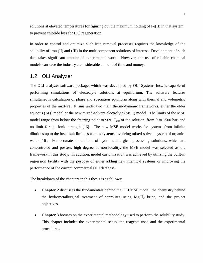
2.3.3 Solubility of Hematite in HCl solutions
The solubility data, which was obtained from literature [1] was converted from molarity to
molality using OLI’s predicted density of the same solution compositions at room temperature.
It was then compared with OLI MSE default model, as seen in Figure 6. Solubility of hematite
increases with increasing HCl concentration. The model showed good agreement at low HCl
concentration (up to 0.3 molal) whereas it overestimated the solubility at higher acid level.
16
Figure 6: Default OLI MSE's simulated solubility of hematite in HCl solutions at 100°C
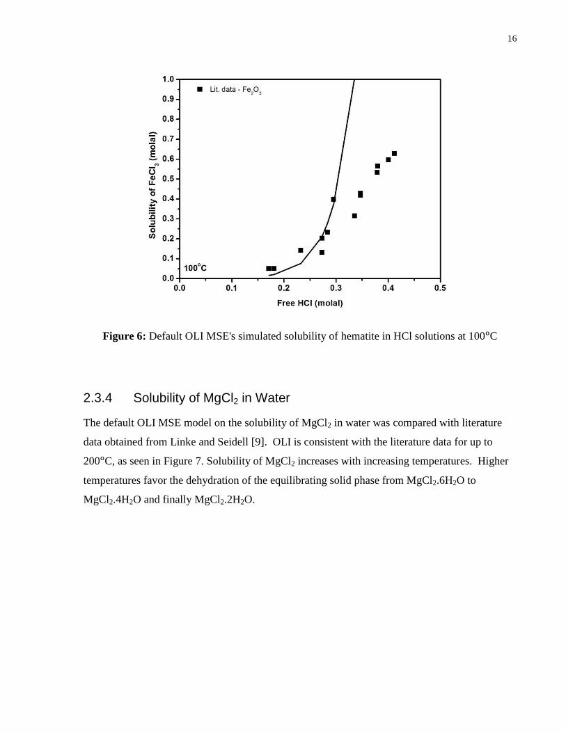
2.3.4 Solubility of MgCl2 in Water
The default OLI MSE model on the solubility of MgCl2 in water was compared with literature
data obtained from Linke and Seidell [9]. OLI is consistent with the literature data for up to
200°C, as seen in Figure 7. Solubility of MgCl2 increases with increasing temperatures. Higher
temperatures favor the dehydration of the equilibrating solid phase from MgCl2.6H2O to
MgCl2.4H2O and finally MgCl2.2H2O.

17
Figure 7: Default OLI MSE's simulated solubility of MgCl2 in water
2.3.5 Solubility of MgCl2 in HCl Solutions
The literature solubility data of MgCl2 in HCl solutions taken from [9] was used to validate the
default OLI MSE model. It can be seen from Figure 8 that the solubility of MgCl2 increases with
increasing temperature but decreases with increasing HCl concentration. The model is in a good
agreement with literature data but OLI overestimates the solubility data at 70°C.

18
Figure 8: Default OLI MSE's simulated solubility of MgCl2 in HCl solutions
2.3.6 Solubility of Hematite in MgCl2 and HCl Solutions
The solubility data was taken from Konigsberger et al. [57]. It was shown in Figure 9 that OLI
default model predicted incorrect solubility trends, i.e. the solubility decreases when MgCl2 is
added as supposed to increase based on the Fe(III) chloride complex formation. The effect of
HCl addition (Figure 10) and temperature (Figure 9 and Figure 10) on the hematite solubility are
captured by the model, but the predicted values are still inaccurate. This identifies a missing
gap in the OLI database.

19
Figure 9: Default OLI MSE's simulated solubility of hematite in MgCl2 solutions with constant
init. HCl at 60 and 90°C. The lines correspond to default OLI MSE's prediction results on the
solubility of hematite

20
Figure 10: Default OLI MSE's simulated solubility of hematite in HCl solutions with constant
init. MgCl2 at 60 and 90°C. The lines correspond to default OLI MSE's prediction on hematite
solubility
2.4 Objectives
The overall objective of this thesis was to optimize and expand the commercial database of iron
(II) and (III) to the conditions of interests to hydrometallurgy, especially from room temperature
up to 100°C and from 0 up to 3 molal of acid (either HCl or H2SO4). The specific objectives
were:
1. Perform solubility experiments on FeCl3-MgCl2-H2O and FeCl3-MgCl2-HCl-H2O systems
from 25°C up to 100°C in order to determine the maximum concentration of Fe(III) during
leaching of saprolitic ore under concentrated magnesium chloride solution
2. Peform solubility experiments on MgCl2-FeCl3-H2O systems from 25 up to 100°C in order to
determine the effect of FeCl3 on the MgCl2 phase diagram, in order to identify an operating
window for magnesium hydroxychloride precipitation.

21
3. Perform solubility experiments of Fe2O3-MgCl2-HCl-H2O systems at 60 and 90°C for
determining the limit of iron removal during iron precipitation step at concentrated MgCl2
solutions through neutralization by MgO addition.
4. Model the new Fe(III) and Mg(II) solubility data on the chloride system through regression
and utilize the developed model to simulate the leaching and iron removal steps.
On the other hand, the secondary objectives of this thesis were:
1. Validate the OLI models on the solubility of Fe(II) and Fe(III) in sulfate or chloride systems
in the presence of acid and/or other metal sulfates/chlorides and compare with literature data.
2. Improve the chemical model by regression of select Fe(II) and Fe(III) systems relevant to
hydrometallurgy

22
Chapter 3
3 Experimental
3.1 Experimental Setup
Low temperature (up to 80°C) FeCl3 solubility in MgCl2 experiments were conducted in
Erlenmeyer flasks immersed in water bath inside an acrylic tank maintained at constant
temperature using Cole Palmer Polystat Digital Immersion Circulator and the solutions were
stirred continuously using magnetic stirrers (See Figure 3-1). The flasks were capped using
rubber stopper equipped with glass thermometer and the vacuum grease was applied to seal the
joints. In addition, parafilm was wrapped around the outer joints of the flasks to enhance the
seal. In order to minimize the evaporation of water from the bath, hollow plastic balls were
added to cover the water surface. For later experiments involving the solubility of MgCl2 in
FeCl3 solutions, as well as the solubility of hematite in acidic MgCl2 solutions, the bath was
modified by replacing the material of the tank with polypropylene, as well as the water bath with
a mixture of polypropylene glycol (PG): water = 70:30 vol% enabling the setup to be used up to
100°C.
Water Bath
60°C
Stirrer
Thermometer
Erlenmeyer
Flask
Magnetic
Stirrer Bar
Thermostat
Rubber
Stopper
Figure 11: Experimental setup for low temperature solubility experiment

23
On the other hand, high temperature (100°C) FeCl3 solubility in MgCl2 experiments were
conducted in 1L jacketed glass reactor heated with oil bath maintained at the reaction
temperature using a VWR temperature-controlled circulator (See Figure 3-2). The stirring was
provided using a motor with the stirrer made of PTFE and the shaft made of glass. A glass
thermometer was attached to the reactor using one of the available top ports to monitor the
temperature. Vacuum grease was applied to seal all of the joints.
Motor
Thermometer
Jacketed
Glass
Reactor
Oil Inlet From
Heater
Oil Outlet to
Heater
Stirrer
Liquid
Sampling Port
Solid Sampling
Port
Figure 12: Experimental setup for high temperature solubility experiment
3.2 Reagents
All the reagents used, i.e. FeCl3.6H2O(s), FeCl3(s), MgCl2.6H2O(s), MgCl2(s), concentrated HCl and
Fe2O3(s) were ACS grade from various chemical suppliers, including Fischer Scientific, Sigma-
Aldrich and Alfa Aesar. The water used for the experiments was Millipore-Q deionized water.

24
3.3 Experimental Procedures
3.3.1 FeCl3 Solubility in MgCl2 Solutions
The solubility experiments were approached from the dissolution pathway. Since the solubility
of FeCl3 increases with temperature, the following procedures were implemented. For
experiments below the melting point of FeCl3.6H2O at 37°C, solutions of various MgCl2
concentrations were prepared using either MgCl2.6H2O or anhydrous MgCl2 and excess
FeCl3.6H2O was added (above its saturation level). On the other hand, for experiments above
37°C, solids containing a predetermined amount of MgCl2.6H2O, FeCl3.6H2O and excess FeCl3
were added to the flasks at ambient temperature and the temperature was raised to the reaction
temperature. This method was selected to control the heat released from the exothermic
dissolution reaction of the anhydrous FeCl3 by melting the FeCl3.6H2O. It prevented the
solutions to boil up which would otherwise cause the experiment to be approached from
supersaturation.
All the equipment used for sampling were kept inside an oven heated slightly above the reaction
temperature to prevent precipitation during sampling. Kinetics studies were performed to
estimate the time required to reach equilibrium. 3 Samples were taken at equilibrium over a
period of 1-2 hours using dip tubes and immediately filtered using a 0.45μm syringe filter. The
supernatant solution was placed in a 1 mL volumetric flask for density measurement at
temperature by measuring its weight using an analytical balance. The resulting solution was
diluted 10-fold using 5% HCl. For experiments involving HCl, the solution was diluted with
deionized water for free acid measurement by an acid-base titration method (See Appendix A-3).
The Fe and Mg concentration were analyzed by using a complexometric titration method (See
Appendix A-1 and A-2, respectively) instead of by ICP-AES due to the error associated with
high dilution from highly concentrated solutions. Solid samples were taken using a dip tube,
filtered using a vacuum filtration apparatus and kept inside vacuum desiccators for phase
analysis by powder X-Ray Diffraction (XRD).
3.3.2 MgCl2 Solubility in FeCl3 Solutions
The solubility experiments were conducted from the dissolution pathways. Since the solubility
of MgCl2 increases with increasing temperature, the experiments were started at 25°C and the

25
temperature was progressively raised up to 100°C. Solutions of various concentration of FeCl3
were prepared and put inside the Erlenmeyer flasks which were kept at 25°C using the water
bath. Following thermal equilibration, excess MgCl2.6H2O was added to the flask marking the
start of the experiment. Initial kinetics was measured to estimate the equilibration time. After
equilibrium was achieved, 2 liquid samples were obtained using a plastic syringe equipped with
a 0.45μm syringe filter and placed inside a 1 mL volumetric flask for density measurement. The
solution was then diluted 10 fold (the first sample in 0.1M HCl solution and the second sample in
DI water to check whether hydrolysis reaction occurs or not). The samples were immediately
titrated for Fe, Mg, and HCl determination using the same method mentioned previously. Solid
samples were obtained as previously mentioned. After sampling, the temperature of the water
bath was raised to the next reaction temperature while ensuring that excess MgCl2.6H2O was
maintained in each flask by visual observation.
3.3.3 Hematite Solubility in Acidic MgCl2 Solutions
The solubility experiments were performed from the dissolution pathway. Solutions containing
MgCl2 and HCl of various concentrations were prepared and initial samples were taken to
confirm the initial solution composition. The solutions were then heated to the reaction
temperature. After thermal equilibrium was achieved, excess Fe2O3 was added to the flasks to
start the solubility experiments. Kinetic tests were performed to estimate the equilibration time.
After equilibrium was achieved, 2 liquid samples were obtained by using dip tubes and
immediately filtered using 0.45 μm syringe filters. The non-diluted solutions remained stable due
to increased solubility with decreasing temperature. For experiments involving saturated MgCl2
solutions, since MgCl2 solubility decreases with decreasing temperature, the filtered solution was
transferred to a 2 mL volumetric flask for density measurement at temperature and immediately
diluted 2.5-fold using deionized water to prevent precipitation of MgCl2.6H2O. Solid samples
were obtained by using dip tubes, and filtered immediately using vacuum filtration apparatus and
stored inside vacuum desiccators. Metals and free acid concentrations were analyzed using the
same methods described in the previous section.

26
Chapter 4
4 Experimental Results and Discussion
4.1 Solubility of FeCl3 in MgCl2 Solutions
4.1.1 Reproducibility Tests for FeCl3 Solubility in Water
Initial tests were performed to reproduce literature data for solubility of FeCl3 in water [9]. As
seen in Figure 13, they show close agreement with the literature up to 60°C and they
underestimate the solubility at 80 and 100°C within 10%.
Figure 13: Reproducibility tests for the solubility of FeCl3 in water
4.1.2 Kinetic Tests for FeCl3 Solubility in MgCl2 solutions
Kinetics were measured at 25°C (see Figure 14) and 40°C (see Figure 15) in order to estimate
the time required for the system to reach equilibrium. At 25°C, the stable solid phase is
FeCl3.6H2O and there is no phase transformation that occurs under the conditions studied.
However, at 40°C, the stable solid phase may differ depending on the conditions, i.e. for no
MgCl2, the stable solid phase is FeCl3.2.5H2O, whereas in the presence of MgCl2, the stable solid

27
phase is the double salt 2.5FeCl3.MgCl2.7.5H2O, which will be described in the later section. It
turns out that the kinetics at 40°C is faster than the kinetics of the phase transformation to the
double salt, indicating that 12 hours is sufficient to reach equilibrium.
Figure 14: Kinetics for FeCl3 solubility in MgCl2 solutions at 25°C

28
Figure 15: Kinetic tests for FeCl3 solubility in MgCl2 solutions at 40°C
4.1.3 FeCl3 Solubility Data in MgCl2 Solutions
The solubility data for FeCl3 in MgCl2 solutions is shown in Figure 16 and Figure 17. It can be
seen that at 25°C the solubility first decreases with increasing MgCl2 concentration due to the
common ion effect; the solubility starts to increase at about 2.5 molal MgCl2 which is due to the
effect of complex formation between Fe3+
and Cl- ions. This complexation effect also explains
the increasing solubility trend at 35°C. Under these conditions, when the equilibrium is
approached from the dissolution pathway, FeCl3.6H2O is the stable solid phase. It is also shown
that the solubility increases with increasing temperature up to 100 °C. At 40°C and above, the
solubility decreases with increasing MgCl2 concentration whereas the stable solid phase under all
conditions studied is the double salt, 2.5FeCl3.MgCl2.7.5H2O. One set of the experiments was
conducted by cooling the equilibrated solutions at 40 °C down to 25 °C. It turns out that the
solubility trends behave similarly with those at above 40 °C and that the double salt remains
stable at 25 °C. The two different solubility values at 25 °C for the same MgCl2 concentrations,
one in equilibrium with the hexahydrate while the other with the double salt, can be traced back
to the nature of the solubility of FeCl3 in water, as seen in Figure 13. It was clear that the phase

29
diagram for FeCl3 in water contains multiple eutectic points, which make it possible to have two
distinct solubility values for the same temperature and solid phase. Thus, it is likely that the
higher solubility values are achieved only when the equilibrium is approached from precipitation
resulting from supersaturated solutions upon cooling from 40 °C back to 25 °C.
Figure 16: Solubility of FeCl3.6H2O in MgCl2 solutions at 25 and 35°C

30
Figure 17: Solubility of 2.5FeCl3.MgCl2.7.5H2O in MgCl2 Solutions from 25 up to 100°C.
Symbols at 0 MgCl2 represent the solubility of FeCl3 hydrates in water.
The XRD spectra for the equilibrating solid phase are included in the Appendix C-1. One
particular feature of the double salt is the unique XRD spectrum which does not correspond to
any FeCl3 solid compound, or any MgCl2 solid compound, as seen in Figure 18. As a
consequence, the identity of the unknown double salt could not be determined by just performing
XRD analysis. In order to resolve this issue, chemical analysis was performed by dissolving the
solid sample in 5% HNO3 and then determining the stoichiometry of the solid phase as follows:
- Metal analysis (Mg, Fe): ICP OES, or complexometric titration
- Chloride analysis: Chloride Ion Selective Electrode (ISE), or gravimetric analysis
- Crystalline water analysis: mass balance. In order to find out whether the only anion is
chloride ion or there is any other anion, e.g. O2-
, OH-, it is simply checked by performing
electroneutrality of the metal cations and chloride anion. If it is electroneutral, all the metals
exist in the form of metal chloride, which is indeed the case. The crystalline water content is
finally determined from mass balance. There are several factors that affect the accuracy of the
measurements:

31
1. The nature of the double salt, a chloride salt which is extremely hygroscopic, thus
absorbing moisture during sample preparation for the analysis and affecting the
crystalline water content of the solid
2. Solid was not washed during filtration due to extreme solubility with any solvents tested,
including water, alcohols, and acetone, which could lead to absorption of the residual
solution on the surface of the double salt, thus affecting the Fe:Mg stoichiometry to vary
between 2.4 up to 3
The complete chemical analysis can be found in Appendix D. The best analysis was performed
by using complexometric titration for Fe and Mg determination, coupled with AgCl gravimetric
analysis for Cl determination which gives the lowest error for the electroneutrality, under 1%.
Finally, the proposed final formula of the double salt is 2.5FeCl3.MgCl2.7.5H2O.

32
Figure 18: XRD Spectra of the double salt from 3 molal init. MgCl2 experiment at 60°C
There were additional attempts to confirm the water content by conducting TGA analysis, as
shown in Appendix D, by measuring the weight difference of crystalline water evaporation, but
this measurement was not clear due to the existence of multiple unidentified peaks, as well as the
high amount of absorbed (not crystalline) water due to the hygroscopic nature of the sample
which blurred the calculation of the crystalline water content based on the weight loss.
4.2 Solubility of MgCl2 in FeCl3 Solutions
4.2.1 Reproducibility Tests for MgCl2 Solubility in Water
The reproducibility check with literature data showed that the results of this work are in an
excellent agreement with the literature solubility data, with errors below 2%, as shown in Figure
19. It clearly indicates that the proposed sampling procedures, as well as the complexometric
titration method for Mg determination work with a high degree of accuracy.

33
Figure 19: Reproducibility tests for the solubility of MgCl2 in Water
4.2.2 Kinetic Tests for MgCl2 Solubility in FeCl3 Solutions
The kinetics of MgCl2.6H2O dissolution in water and in 0.5 molal FeCl3 even at 25°C is very fast
with equilibrium attained in less than 4 hours, as seen in Figure 20. However, for each
experiment, even at higher FeCl3 concentrations, up to 2 molal, 12 hours of holding time was
chosen to ensure that the solutions have reached equilibrium.

34
Figure 20: Kinetic Tests for Solubility of MgCl2 in FeCl3 Solutions
4.2.3 MgCl2 Solubility in FeCl3 Solutions
The solubility of MgCl2 decreases with increasing FeCl3 concentration which is due to the
common ion effect and increases with increasing temperature, as seen in Figure 21. However,
the decrease of the solubility diminishes with increasing temperature. At 100°C, the effect of
FeCl3 addition has no significant impact (just under 5%) on the decrease of solubility of MgCl2.
The solid phase was identified by XRD as MgCl2.6H2O; details are included in Appendix C-2.

35
Figure 21: Solubility of MgCl2 in FeCl3 Solutions from 25 up to 100°C
4.3 Solubility of Hematite in MgCl2 and HCl Solutions
4.3.1 Reproducibility of Hematite Solubility in MgCl2 and HCl Solutions
Tests were also performed to check if we could reproduce hematite solubility data in MgCl2 and
HCl as measured by Konigsberger [57]. However, the results were inconsistent due to HCl loss
to the vapor phase. HCl loss affects the mass balance calculation as well as the extent of
hematite dissolution. It becomes worse when the concentration of the chloride brines and the
temperature is high as seen by the difference between the measured vs. calculated lines in Figure
4-9. Vapor-Liquid Equilibria of HCl in MgCl2 solutions, as seen in Figure 23, has been studied
in the literature [58] and it has been shown that chloride addition promotes the formation of
molecular HCl which is in equilibrium with the HCl vapor based on the following reaction:
H+ (aq) + Cl
- (aq) → HCl (aq) → HCl (g) (4-11)
which makes it possible to distill HCl(g) using very concentrated chloride brines.

36
Figure 22: Reproducibility issues in the solubility of hematite in MgCl2 and HCl solutions
Figure 23: Vapor-Liquid Equilibria of HCl in MgCl2 Solutions

37
The main sources of error come from:
1. HCl losses during initial sampling at temperature and prior to adding the hematite
powder,
2. HCl losses during sampling (kinetic or equilibrium), and
3. High solubility of hematite in MgCl2 brines which leaves a very small residual free
HCl at equilibrium.
The above cause the measured initial HCl to be overestimated, the equilibrium HCl to be
underestimated, and the free acid measurement by titration to be less reliable. Konigsberger et
al., in performing their hematite solubility measurements used a recycled plug flow reactor
(PFR) with hematite placed in a fixed bed [59], which in theory prevents supersaturation due to
excessive stirring. They successfully closed the mass balance by using a pH electrode specially
calibrated with respect to the concentration (as opposed to activity) of H+ and at constant MgCl2
concentration [57]. This sophisticated continuous measurement of the free acid cannot be
reproduced inside a batch reactor due to the need to separate the supernatant from the solid to
prevent buildup of hematite powder on the tip of the pH probe.
4.3.2 Kinetic Tests for Hematite Solubility in MgCl2 and HCl Solutions
Figure 24 shows that the kinetics of hematite dissolution reaches equilibrium in 24 hours in the
absence of MgCl2. On the other hand, the kinetics is faster with increasing MgCl2 concentration
due to an increase of the activity of proton in these water-deprived systems.

38
Figure 24: Kinetic tests for hematite solubility in 0.1 molal HCl initially and varying MgCl2
concentration
4.3.3 Hematite Solubility Data in MgCl2 and HCl Solutions
Despite the inability of the current measurements to obtain solubility data at prescribed acid
concentration levels due to HCl losses, several trends can be observed. The new hematite
solubility in MgCl2 and HCl solutions, as seen in Figure 25 shows that MgCl2 addition increases
the solubility of hematite, as previously confirmed by Konigsberger [57] up to 4 molal and then
decreases as the MgCl2 concentration approaches its saturation level. The increase of the
solubility is due to ferric chloride complex formation and the decrease is due to salting out effect,
at which there is no more available water to hydrate the Fe3+
ions in the solution. This salting
out effect seems to have a more pronounced effect at higher HCl concentration. The solubility of
hematite also decreases with increasing temperature, which is also consistent with the
Konigsberger's observation [57]. The XRD spectra for the equilibrating solid phases are
included in Appendix C-3.

39
Figure 25: Solubility of hematite in MgCl2 and HCl solutions at 60 and 90°C

40
Chapter 5
5 OLI Modeling Results and Discussion
5.1 Fitting on the FeCl3-MgCl2-H2O System
The default OLI model has successfully simulated the binary and ternary chloride systems of
interests: FeCl3-H2O, MgCl2-H2O, FeCl3-HCl-H2O, MgCl2-HCl-H2O, but not for the system
FeCl3-MgCl2, as seen previously in Chapter 2.3. The new solubility data of FeCl3 in MgCl2
solutions, as well as the MgCl2 in FeCl3 solutions, was fitted on the OLI MSE model and several
parameters were regressed. First, the basic thermodynamic properties of the new double salt,
2.5FeCl3.MgCl2.7.5H2O was regressed, i.e. ΔG°f, S° and heat capacity of the solid, Cp, since this
solid compound is new and there is no published thermodynamic parameters of the salt. Second,
the mid-range binary interaction parameters between major species in the solution, FeCl2+
- Mg2+
and FeCl2+
- Mg2+
were regressed as well. The regressed parameters and the comparison
between the thermodynamic properties of the new double salt and the 3 form of the magnesium
hydroxychloride are shown in Table 1 and Table 2, respectively. It was clear that the regressed
thermodynamic parameters of the new double salt is in the same order of magnitude with the “3-
form” of the magnesium hydroxychloride.
Table 1: Regressed OLI parameters for FeCl3-MgCl2-H2O system
Species Standard State Properties BMD CMD
2.5FeCl3.MgCl2.
7.5H2O(s)
ΔG°f = -3.379986 MJ/mol
S° = 0.64759 kJ/mol.K
ΔH°f = -4.054028 MJ/mol
Cp = 52.189 J/mol.K
- -
FeCl2+
- Mg2+
- BMD0 = 218.3465 CMD0 = -472.2865

41
BMD1 = -0.545778
BMD2 = 16731.82
CMD1 = 0.9531058
CMD2 = 3236.161
FeCl2+
- Mg2+
- BMD0 = 1333.926
BMD1 = -2.607153
BMD2 = -67653.59
CMD0 = -581.7210
CMD1 = 1.652331
CMD2 = -138093.5
Table 2: Comparison of the thermodynamic properties of the double salts
Solid species ΔG°f (kJ/mol) S° (J/mol.K) Cp (kJ/mol.K)
2.5FeCl3.MgCl2.7.5H2O -3379.86 647.59 52.189
3MgO.MgCl2.11H2O [5] -6077.45 643 -
It could be seen in Figure 26, Figure 27 and Figure 28 that the OLI model is consistent with both
systems FeCl3-MgCl2-H2O and MgCl2-FeCl3-H2O with AARD less than 5%. The fitted model
was then validated using the new solubility of FeCl3 in the presence of MgCl2 and HCl solutions
within around 3% error, as presented in Figure 29.

42
Figure 26: OLI fitting on the solubility of FeCl3.6H2O in MgCl2 solutions
Figure 27: OLI fitting on the solubility of 2.5FeCl3.MgCl2.7.5H2O in MgCl2 solution. The
dashed lines represent the solubility of FeCl3 hydrates at low MgCl2 concentration.

43
Figure 28: OLI fitting on the solubility of MgCl2 in FeCl3 solutions
Figure 29: OLI prediction on the solubility of FeCl3 in MgCl2 and HCl solutions

44
5.2 Maximum Achievable Solid Loading during Leaching
The high solubility of FeCl3 in MgCl2 brines enables processing of saprolite ores with minimum
amount of solution, thus potentially reducing the overall equipment sizes. A previous
experimental study on leaching of saprolite under MgCl2 brines was conducted up to 25% solid
loading by using HCl gas instead of concentrated HCl(aq) [6]. Mined saprolite comes often in
the form of a slurry with about 30% solids. Since Ni dissolution follows Fe dissolution from
saprolite, it is expected that in order to achieve near complete (>99%) extraction of Ni, all Fe
should be dissolved. Due to the high chloride strength of the brine, Fe in-situ hydrolytic
precipitation as hematite is hindered. Therefore, estimation of the maximum achievable solid
loading is based on how much Fe can be dissolved without precipitation of any chloride salt,
mainly as FeCl3. Calculation of solids loading was performed using the ore composition as in
Table 5-2:
Table 3: Saprolite Ore Composition (Dry Basis) [6]
Metal Ni Co Fe Mg Al Mn Cr
Wt % 3.89 0.07 25.47 3.12 0.60 0.44 0.41
The MgCl2 brine strength of 2 and 4.5 molal was chosen as the constituent of the liquid phase
during calculation of the solid loading which represents the brine strength used in the previous
study during leaching step [6]. The maximum Fe dissolution data from Table 4 was used to
construct the dissolved iron curve in Figure 30. This information, combined with the OLI model
prediction of FeCl3 solubility in 2 or 4.5 molal MgCl2 and 0 up to 1 molal HCl solutions at
100°C would serve as the way to estimate the maximum solid loading, i.e. to have the solid
loading curve just below the solubility limit of the double salt. For 2 and 4.5 molal MgCl2, the
maximum solid loading was estimated to be around 75% and 60%, respectively.

45
Table 4: Theoretical maximum dissolution of Fe, Ni, and Mg based on the solid loading
MgCl2 (molal) Solid Loading
(%)
Maximum Fe
(molal)
Maximum Ni
(molal)
Maximum Mg
(molal)
2 35 2.92 0.42 0.82
2 50 5.43 0.79 1.53
2 75 16.29 2.37 4.58
4.5 35 3.51 0.51 0.99
4.5 50 6.51 0.95 1.83
4.5 60 9.77 1.42 2.75
Figure 30: Maximum solid loading achievable based on OLI Prediction

46
However, in practice, the selection of maximum solid loading is much lower than the theoretical
maximum solid loading because the process is bound to the MgCl2 phase diagram. As MgO is
used as neutralizing agent, more MgCl2 is introduced to the solution, thus further augmenting the
brine concentration. The limit of how much MgCl2 can be dissolved without losing any chloride
unit depends on the knowledge of the phase diagram of MgCl2. In this case, there are several
factors that influence the increase of the MgCl2 concentration, some of which are controllable
and the rest are not, as follows:
- Selection of the starting MgCl2 brine concentration prior to leaching step (controllable)
- Mg dissolution from the saprolite ores (uncontrollable)
- Free acid neutralization reaction: MgO (s) + 2HCl (aq) = MgCl2 (aq) + H2O (l) (controllable)
- Iron precipitation reaction: 3MgO (s) + 2FeCl3 (aq) = 3MgCl2 (aq) + Fe2O3 (s) (uncontrollable)
- Nickel precipitation reaction: MgO (s) + NiCl2 (aq) = MgCl2 (aq) + NiO (s) (uncontrollable)
The biggest factor that influences the increase of MgCl2 concentration in the solution is the iron
precipitation reaction which has 3:2 stoichiometry with respect to MgCl2:FeCl3. Since the
solution is dominated by iron, according to the stoichiometry, precipitating all iron from the
solution significantly increases the MgCl2 concentration. Starting the leaching step with 4.5
molal MgCl2 brine would make it difficult to operate with high solid loading because of the
solubility limit of MgCl2 in water, around 7.7 molal at 100°C. As a result, it would be more
reasonable to operate at lower starting MgCl2 at around 2 molal (or possibly lower) and then to
neutralize the solution to precipitate the iron and nickel before reaching the solubility limit of
MgCl2. With all of these factors taken into consideration, the maximum operable solid loading
decreases to around 35% when leaching is performed at 2 molal MgCl2 brine at 100°C. Below is
the summary of the MgCl2 increase from leaching up to the end of Ni precipitation:
- Starting MgCl2 brine concentration = 2 molal
- Mg dissolution (assuming 50% extraction) = 0.41 molal
- Free acid neutralization (assuming 0.5 molal free acid) = 0.25 molal

47
- Iron removal through MgO neutralization = 4.38 molal
- Ni removal through MgO neutralization = 0.42 molal
- Total = 7.46 molal
The resulting MgCl2 concentration is still just below the solubility limit of MgCl2 in water at
100°C and meets the requirement of at least 30 wt% MgCl2 concentration (4.5 molal) for
magnesium hydroxychloride precipitation. This process could be further improved by lowering
the initial MgCl2 brine concentration below 2 molal to accomodate for possible higher Mg
extraction from the ore as well as lower free acid concentration. Nevertheless, solid loading of
35% is possible to be processed under the proposed saprolite processing circuit.
5.3 Effect of FeCl3 Addition on MgCl2 Phase Diagram
Addition of FeCl3 decreases the solubility of MgCl2 due to common ion effect and it can be seen
from Figure 31. The decrease in the MgCl2 solubility is smaller at higher temperature. However,
the boiling point of the solution keeps rising with additional FeCl3. This could potentially affect
the operating window for magnesium hydroxychloride precipitation. These two contradicting
effects seem to have a neutral effect on the process operating window. In the proposed process,
prior to Fe removal, the system is expected to have high concentration of dissolved FeCl3 but as
more FeCl3 is precipitated through MgO addition, the phase diagram would eventually shift back
to the MgCl2-H2O phase diagram. At any point of time during Fe removal, the MgCl2
concentration should never fall above the solubility limit of MgCl2 in FeCl3 solution and this
could be prevented by good selection of process conditions as outlined in the previous section.

48
Figure 31: OLI's Predicted MgCl2-FeCl3-H2O ternary phase diagram
5.4 Limitation of The OLI Model
While the developed OLI model for the system FeCl3-MgCl2-HCl-H2O performs well, it suffers
from a lack of accuracy when used in predicting the solubility of hematite in HCl, as well in the
presence of MgCl2. As seen in Figure 32, the solubility of hematite increases with increasing
free HCl concentration and decreases with increasing temperature. When compared with the
solubility data obtained from Dutrizac and Riveros, their solubility data seems to be higher than
that of obtained from this work at 60 and 90°C.

49
Figure 32: Predicted solubility of hematite in HCl solutions
Their overestimated data is mainly due to their equilibrium approach from hydrolytic
precipitation of FeCl3 instead of hematite dissolution. The developed OLI model predicted the
correct trends when compared with the results of this work for the system Fe2O3-HCl. When the
model is used to predict hematite solubility in MgCl2 and HCl solutions, it underestimated the
solubility data by around 1 log unit, as seen in Figure 33. Nevertheless, the model still predicted
the correct trends for MgCl2 addition to the hematite solubility, i.e. the solubility increases with
MgCl2 addition due to ferric chloride complex formation, as clearly seen in Figure 33. This
limitation may be due to the absence of higher order complexes, FeCl3(aq) and FeCl4- in the
default OLI database. The default FeCl3-H2O and FeCl3-HCl-H2O was built using only the first
two ferric chloride complexes, i.e. FeCl2+ and FeCl2
+ and it manages to performs well in the
system FeCl3-MgCl2-H2O as well as FeCl3-MgCl2-HCl-H2O. However, when the higher order
complexes are introduced to the OLI database, it would disrupt the performance of the all the
developed FeCl3 models and as a result, refitting of the whole FeCl3 system starting from the
binary FeCl3-H2O may be required. Furthermore, regressing more interaction parameters requires
more data points to prevent over-parameterization. This approach, which may further improve
the overall performance of the model, may be the subject for a future study.

50
Figure 33: Predicted solubility of hematite in MgCl2 and HCl solutions

51
Figure 34: Predicted hematite solubility in MgCl2 solutions at const. free HCl
5.5 OLI Model Improvement for Other Fe(II) and Fe(III) Systems
OLI model improvement was performed on select Fe(II) and Fe(III) systems, relevant in
hydrometallurgy which is included in Appendix E. A summary of all the improvements is as
follows:
Table 5: Summary of improved OLI model on Fe(II) and Fe(III) systems
Type of System Temperature Range (°C) AARD (%)
FeSO4-H2O 25-220 9.16
FeSO4-H2SO4-H2O 25-100 6.58
FeSO4-H2SO4-H2O 160-220 4.45
FeSO4-MgSO4-H2O 25-90 9.74

52
FeSO4-MgSO4-H2SO4-H2O 200 12.76
FeSO4-ZnSO4-H2SO4-H2O 140-180 -
FeSO4-ZnSO4-H2SO4-H2O 200 7.33
FeCl2-HCl-H2O 25-100 1.81
FeCl2-MgCl2-H2O 25-90 5.64
FeCl2-MgCl2-HCl-H2O 50 14.66
Fe2O3-H2SO4-H2O 130-170 20.2
Fe2O3-H2SO4-H2O 230-270 23.8
Fe2O3-MgSO4-H2SO4-H2O 250 11.5
NaFe3(SO4)2(OH)6 70-110 12.9

53
Chapter 6
6 Conclusions
Chemical modeling of Fe(II)/(III) in hydrometallurgy using OLI was investigated in this work
with the focus on modeling of FeCl3-MgCl2-HCl-H2O system relevant in hydrometallurgical
treatment of saprolitic laterites using MgCl2 brines. The conclusions of this work are as follows:
1. The solubility of FeCl3 in MgCl2 solutions was investigated in this work from 25°C up to
100°C and up to 4.5 molal MgCl2. It was found out that the solubility increases with
increasing temperature but it decreases with increasing MgCl2 concentration for the
temperature range of 40 to 100°C due to common ion effect. However, the solubility
below 40°C, especially at 25°C shows two opposite trends with the addition of MgCl2.
The solubility first decreases due to common ion effect and then it increases at higher
concentration of MgCl2 due to Fe3+
-Cl- complex formation. In the presence of MgCl2,
the stable solid phase below 37°C is FeCl3.6H2O while a new type of double salt,
2.5FeCl3.MgCl2.7.5H2O was identified at temperature as low as 25°C and up to 100°C.
2. The solubility of MgCl2 in FeCl3 solutions was experimentally investigated in this work
from 25°C up to 100°C and up to 2 molal FeCl3. It was observed that the solubility
increases with increasing temperature but it decreases with increasing FeCl3
concentration due to common ion effect. Furthermore, the decrease of the solubility with
FeCl3 addition diminishes with increasing temperature. Under all conditions studied, the
stable solid phase is always MgCl2.6H2O.
3. The solubility of hematite in MgCl2 and HCl solutions was experimentally determined in
this work at 60 °C and 90 °C and it further extends the concentration range of literature
data previously produced by Konigsberger et al. [57] up to the saturation limit of MgCl2.
Despite the experimental difficulties associated with HCl losses to the vapour, which
prevents from closing the mass balance, several meaningful trends were observed when
the equilibrium HCl was determined from mass balance, not from measurements. It was
observed that the solubility of hematite decreases with increasing temperature but
drastically increases with MgCl2 concentration due to the formation of Fe3+
-Cl-

54
complexes. However, at MgCl2 concentration above 4 m and up to saturation, the
solubility of hematite drops suggesting that there is a common-ion effect at higher MgCl2
concentration. Further investigations are necessary for understanding the solubility
trends of hematite at more concentrated MgCl2 solutions.
4. The default OLI MSE database reproduces literature data on binary chloride systems
(FeCl3-H2O and MgCl2-H2O) and ternary chloride systems (FeCl3-HCl-H2O and MgCl2-
HCl-H2O). The missing binary FeCl3-MgCl2 system was required for good prediction in
the quaternary FeCl3-MgCl2-HCl-H2O. The experimental data on the solubility in the
FeCl3-MgCl2 that was obtained from this work was fitted on the OLI MSE model in order
to obtain new interaction parameters between Fe3+
and Mg2+
species, as well as the
standard state properties of the double salt, 2.5FeCl3.MgCl2.7.5H2O. The model was
found to be valid when compared with experimental solubility data on the quaternary
system obtained from this work not used in the parameterisation.
5. Due to the high solubility of most metal chlorides, it was possible to further increase the
solid loading during leaching with the purpose of reducing the processing equipment
sizes. Since Fe2O3 hydrolytic precipitation during leaching is inhibited by concentrared
MgCl2 brines and the fact that Ni dissolution follows Fe dissolution from the ore, the
process throughput is limited by FeCl3 solubility in the MgCl2 brine solutions under a
given free HCl concentration. Calculations were performed using the developed model to
predict the maximum solids loading that can be achieved without losing the chloride units
pertinent to HCl recovery step. It was estimated that considering the leaching step only,
up to 75% solid loading can be processed in 2 molal MgCl2 brines. However, since MgO
is used to neutralize the free HCl and precipitate Fe, Ni, Co, the MgCl2 concentration
would keep increasing throughout the process and as a result the ultimate limiting factor
will be the MgCl2 solubility. Thus, the operable solid loading is around 35%, which is
far below the predicted FeCl3 solubility.
6. Since FeCl3 addition decreases the solubility of MgCl2, but it further elevates the boiling
point of the solution, the operating window for magnesium hydroxychloride remains
unchanged. However, as Fe is removed from the solution by MgO addition, it is
expected that at the end of Fe removal, the system will approach the solubility of MgCl2

55
in water. Maintaining the MgCl2 level below the solubility limit at any given time during
MgO addition is necessary to prevent premature chloride unit loss.
7. The predicted OLI MSE model on hematite solubility in MgCl2 and HCl solutions is still
far below the literature values. This could be due to the fact that only the first two Fe3+
-
Cl- complexes (FeCl
2+ and FeCl2
+) were considered during the development of the default
OLI MSE model. Addition of the higher order complexes may improve the overall
performance of the model but reworking of the whole FeCl3 system is required.

56
Chapter 7
7 Recommendation for Future Work
Further improvements are required in some aspects of the present work as follows:
1. Further analysis of the double salt, 2.5FeCl3.MgCl2.7.5H2O is required to obtain the exact
stoichiometry since this salt is extremely soluble in any common solvent used in solid
washing, i.e. H2O, alcohols, and acetone. The fact that solid washing was not performed
during this study could result in metal absorption to the surface of the solid, thus affecting
its overall stoichiometry. Furthermore, this compound is very hygroscopic and thus may
further increase the water content during chemical and TGA analysis. Analysing
conditions in the absence of moisture may be required.
2. Hematite solubility in the presence of MgCl2 and HCl needs to be performed in
pressurized vessels in order to suppress the volatility of HCl in the MgCl2 brines. This
could improve the measurement of free HCl and close the mass balance with high degree
of accuracy.
3. OLI Modeling of hematite in MgCl2 and HCl solutions may be further improved by
reworking the whole FeCl3 system, starting from the binary system by adding the higher
order Fe3+
-Cl- complexes not available yet in the OLI MSE default database.

57
References
[1] J. E. Dutrizac and P. A. Riveros, “The precipitation of hematite from ferric chloride media
at atmospheric pressure,” Metallurgical and Materials Transactions B, vol. 30B, pp. 993-
1001, 1999.
[2] J. E. Dutrizac and J. L. Jambor, “Jarosites and their application in hydrometallurgy,” in
Reviews in Mineralogy and Geochemistry, vol. 40, C. N. Alpers, J. L. Jambor and D. K.
Nordstrom, Eds., Washington D.C., Mineralogical Society of America, 2000, pp. 405-451.
[3] D. Paktunc and J. E. Dutrizac, “Characterization of arsenate-for-sulphate substitution in
synthetic jarosite using x-ray diffraction and x-ray absorption spectroscopy,” The Canadian
Mineralogist, vol. 41, pp. 905-919, 2003.
[4] A. D. Dalvi, W. G. Bacon and R. C. Osborne, “The past and the future of nickel laterites,”
in PDAC 2004 International Convention, Toronto, 2004.
[5] J. S. Bakker, “The recovery of magnesium oxide and hydrogen chloride from magnesium
chloride brines and molten salt hydrates,” Kingston, 2011.
[6] D. Duffy, V. G. Papangelakis and B. Davis, “Saprolite leaching and iron precipitation in
magnesium chloride brine,” in COM 2012, Towards Clean Metallurgical Processing for
Profit, Social and Environmental Stewardship, Niagara Falls, ON, 2012.
[7] A. Onozaki, K. Sato and S. Kuramochi, “Effect of some impurities on iron precipitation at
the Iijima Zinc Refinery,” in Iron Control in Hydrometallurgy, J. E. Dutrizac and A. J.
Monhemius, Eds., Chichester, Ellis Horwood, 1986, pp. 742-752.
[8] T. Yamada, H. Nagata, A. Hosoi, M. Kato and R. Togashi, “Recent improvement of
electrolytic zinc production at Iijima Refinery,” in Zinc & Lead '95, T. Akazami, N.
Masuko, J. E. Dutrizac and E. Ozberk, Eds., Tokyo, The Mining & Materials Processing
Institute of Japan, 1995, pp. 589-598.

58
[9] W. F. Linke and A. Seidell, Solubilities, inorganic and metal-organic compounds vol. I & II,
New Jersey: Van Nostrand Company, 1958 & 1965.
[10] V. G. Bruhn, J. Gerlach and F. Pawlek, “Untersuchungen uber die loslichkeiten von salzen
und gasen in wasser und wabrigen losungen bei temperaturen oberhalb 100 C,” Zeitschrift
fur anorganische und allgemeine chemie, vol. 337, pp. 68-79, 1965.
[11] F. Hasegawa, K. Tozawa and T. Nishimura, “Solubility of ferrous sulfate in aqueous
solutions at high temperatures,” Shigen to Sozai, vol. 112, no. 12, pp. 879-884, 1998.
[12] T. C.-M. Cheng, “Production of hematite in acidic zinc sulphate media,” Montreal, 2002.
[13] M. Regel-Rosocka, “A review of methods of regeneration of spent pickling solutions from
steel processing,” Journal of Hazardous Materials, vol. 177, pp. 57-69, 2010.
[14] B. Harris, C. White and B. Ballantyne, “Chloride leaching of polymetallic massive
sulphide,” in ALTA Copper 10, Perth, 2006.
[15] G. B. Harris, C. W. White, G. P. Demopoulos and B. Ballantyne, “Recovery of copper from
a massive polymetallic sulphide by high concentration chloride leaching,” Canadian
Metallurgical Quarterly, vol. 47, no. 3, pp. 347-356, 2008.
[16] P. Wang, A. Anderko and R. D. Young, “A speciation-based model for mixed-solvent
electrolyte systems,” Fluid Phase Equilibria, vol. 203, pp. 141-176, 2002.
[17] Honeywell, “Unisim Design OLI Interface,” 2010.
[18] H. C. Helgeson and D. H. Kirkham, “Theroretical prediction of the thermodynamic
properties of aqueous electrolytes at high pressures and temperatures. I & II.,” American
Journal of Science, vol. 274, pp. 1089-1198 & 1199-1261, 1974.
[19] H. C. Helgeson and D. H. Kirkham, “Theoretical prediction of thermodynamic properties of
aqueous electrolytes at high pressures and temperatures. III. Equation of state for aqueous
species at infinite dilution.,” American Journal of Science, vol. 276, pp. 97-240, 1976.

59
[20] H. C. Helgeson, D. H. Kirkham and G. C. Flowers, “Theoretical prediction of the
thermodynamic behavior of aqueous electrolytes at high pressures and temperatures. IV.
Calculation of activity coefficient, and apparent molal and standard and relative partial
molal properties to 600 degrees C and 5kb,” American Journal of Science, vol. 281, pp.
1249-1516.
[21] E. L. Shock and H. C. Helgeson, “Calculation of the thermodynamic and transport
properties of aqueous species at high pressures and temperatures: correlation algorithms for
ionic species and equation of state predictions to 5kb and 1000 degrees C,” Geochimica et
Cosmochimica Acta, vol. 52, pp. 2009-2036, 1988.
[22] E. L. Shock and H. C. Helgeson, “Calculation of the thermodynamic and transport
properties of aqueous species at high pressures and temperatures: standard partial molal
properties of organic species,” Geochimica et Cosmochimica Acta, vol. 54, pp. 915-945,
1990.
[23] E. L. Shock, H. C. Helgeson and D. A. Sverjensky, “Calculation of the thermodynamic and
transport properties of aqueous species at high pressures and temperatures: standard partial
molal properties of inorganic neutral species,” Geochimica et Cosmochimica Acta, vol. 53,
pp. 2157-2183, 1989.
[24] E. L. Shock, D. C. Sasani, M. Willis and D. A. Sverjensky, “Inorganic species in geologic
fluids: correlations among standard molal thermodynamic properties of aqueous ions and
hydroxide complexes,” Geochimica et Cosmochimica Acta, vol. 61, pp. 907-950, 1997.
[25] D. A. Sverjensky, E. L. Shock and H. C. Helgeson, “Prediction of the thermodynamic
properties of aqueous metal complexes to 1000 degrees C and 5kb,” Geochimica et
Cosmochimica Acta, vol. 61, pp. 1359-1412, 1997.
[26] K. S. Pitzer, “Thermodynamics of electrolytes. I. Theoretical basis and general equations,”
Journal of Physical Chemistry, vol. 77, pp. 268-277, 1973.
[27] K. S. Pitzer, “Electrolytes. From dilute solutions to fused salts,” Journal of American

60
Chemical Society, vol. 102, pp. 2902-2906, 1980.
[28] C. Achard, C. -G. Dussap and J. -B. Gros, “Prediction of pH in complex aqueous mixtures
using a group-contribution method,” American Institute of Chemical Engineers Joudnal,
vol. 40, pp. 1210-1222, 1994.
[29] C. -C. Chen, H. I. Britt, J. F. Boston and L. B. Evans, “Local composition model for excess
Gibbs energy of electrolyte systems. Part I: single solvent, single completely dissociated
electrolyte systems,” American Institute of Chemical Engineers Journal, vol. 28, pp. 588-
596, 1982.
[30] C. -C. Chen and L. B. Evans, “A local composition model for the excess Gibbs energy of
aqueous electrolyte systems,” American Institute of Chemical Engineers Journal, vol. 32,
pp. 444-454, 1986.
[31] K. S. Pitzer and J. M. Simonson, “Thermodynamics of multicomponent, mixcible, ionic
systems: theory and equations,” Journal of Physical Chemistry, vol. 90, pp. 3005-3009,
1986.
[32] Y. Liu and S. Watanasiri, “Representation of liquid-liquid equilibrium of mixed-solvent
electrolyte systems using the extended electrolyte NRTL model,” Fluid Phase Equilibria,
vol. 116, pp. 193-200, 1996.
[33] S. P. Pinho and E. A. Macedo, “Representation of salt solubility in mixed solvents: a
comparison of thermodynamic models,” Fluid Phase Equilibria, vol. 116, pp. 209-216,
1996.
[34] P. Wang, R. D. Springer, A. Anderko and R. D. Young, “Modeling phase equilibria and
speciation in mixed-solvent electrolyte systems,” Fluid Phase Equilibria, Vols. 222-223, pp.
11-17, 2002.
[35] F. Stober, C. Walker, N. Voermann, M. Solar and B. Wasmund, “Evolution and future of
Rotary Kiln-Electric Furnace (RKEF) plants for smelting of nickel laterites,” in ALTA
Nickel/Cobalt Conference, Perth, 2008.

61
[36] J. Kyle, “Nickel laterite processing technologies - where to next?,” in ALTA 2010
Nickel/Cobalt/Copper Conference, Perth, 2010.
[37] A. J. Moyes, “The Intec Nickel Laterite Process,” in ALTA 2005 Ni/Co 10, Perth, Australia,
2005.
[38] B. Harris and J. Magee, “Atmospheric chloride leaching:the way forward for nickel
laterites,” in Hydrometallurgy 2003, Vancouver, 2003.
[39] G. B. Harris, T. J. Magee, V. I. Lakshmanan and R. Sridhar, “The Jaguar Nickel Inc. Sechol
Laterite Project atmospheric chloride leach process,” in Proceedings of International
Laterite Nickel Symposium 2004, W. P. Imrie and D. M. Lane, Eds., Charlotte, 2004, p. 219.
[40] J. T. Smit and J. D. T. Steyl, “Leaching process in the presence of hydrochloric acid for the
recovery of a value metal from an ore”. Patent WO2006043158, 27 April 2006.
[41] J. J. Jansz, “Estimation of ionic activities in chloride systems at ambient and elevated
temperatures,” Hydrometallurgy, vol. 11, pp. 13-31, 1983.
[42] G. P. Demopoulos, Z. Li, L. Becze, G. Moldoveanu, T. C. Cheng and B. Harris, “New
technologies for HCl regeneration in chloride hydrometallurgy,” World of Metallurgy -
ERZMETALL, vol. 61, no. 2, pp. 89-98, 2008.
[43] R. G. McDonald and B. I. Whittington, “Atmospheric acid leaching of nickel laterites
review. Part II. Chloride and bio-technologies,” Hydrometallurgy, vol. 91, pp. 56-69, 2008.
[44] B. Harris, C. White, M. Jansen and D. Pursell, “A new approach to the high concentration
chloride leaching of nickel laterite,” in ALTA Ni/Co 11, Perth, WA, 2006.
[45] B. Harris, “Continuing development of the Jaguar Nickel Sechol laterite Project in
Guatemala,” in Second New Caledonian Nickel Conference, Noumea, 2004.
[46] R. T. Poy, “Regeneration of hydrochloric acid from ferrous chloride using the
Keramchemie/Lurgi Fluidized Bed Reactor System,” in Iron Control and Disposal, Second

62
International Symposium on Iron Control in Hydrometallurgy, J. E. Dutrizac and G. B.
Harris, Eds., Ottawa, 1996, p. 471.
[47] E. M. Peek, O. F. Goedhart and G. V. Weert, “Process evaluation of steel pickle liquor
pyrohydrolysis in a commercial Keramchemie Fluid Bed Reactor,” in Iron Control and
Disposal, Second International Symposium on Iron Control in Hydrometallurgy, J. E.
Dutrizac and G. B. Harris, Eds., Ottawa, 1996, p. 483.
[48] F. Baerhold, A. Lebl and J. Statrcevic, “Recycling of spent acids and iron via
pyrohydrolysis,” in Iron Control Technologies, Proceedings of the Third International
Symposium on Iron Control in Hydrometallurgy, 36th Annual CIM Hydrometallurgical
Meeting, J. E. Dutrizac and P. A. Riveros, Eds., Montreal, 2006, p. 789.
[49] K. Adham, C. Lee and D. Small, “Energy consumption for iron chloride pyrohydrolysis: a
comparison between fluid beds and spray roasters,” in Iron Control Technologies,
Proceedings of the Third International Symposium on Iron Control in Hydrometallurgy,
36th Annual CIM Hydrometallurgical Meeting, J. E. Dutrizac and P. A. Riveros, Eds.,
Montreal, 2006, p. 815.
[50] B. Harris, C. White, G. Demopoulos and L. Becze, “Recovery of metal oxides and
associated acid from process solutions using water as reagent,” in ALTA Copper 2008,
Perth, 2008.
[51] L. Becze, S. J. Hock and G. P. Demopoulos, “Precipitation of hematite and recovery of
hydrochloric acid from concentrated iron chloride solutions by a novel hydrolytic
decomposition process,” in EPD Congress 2011, 2011.
[52] B. Harris and C. White, “Recent developments in the chloride processing of nickel
laterites,” in ALTA 2011, Perth, 2011.
[53] J. W. Burtch, “PORI hydrochloric acid regeneration process,” Iron and Steel Engineer, vol.
50, no. 4, p. 40, 1973.
[54] J. W. Burtch, “PORI hydrochloric acid regeneration process,” SEAISI Quarterly, vol. 2, no.

63
4, p. 52, 1973.
[55] J. W. Burtch, “Hydrochloric acid from industrial waste streams - the PORI Process,” CIM
Bulletin, vol. 68, p. 96, January 1975.
[56] J. W. Burtch, “Regeneration of hydrochloric acid from spent pickle liquor,” Wire Journal,
vol. 9, no. 2, p. 57, 1976.
[57] E. Konigsberger, L. -C. Konigsberger, P. May and B. Harris, “Properties of electrolyte
solutions relevant to high concentration chloride leaching. III. Solubility of pertinent solids
and iron(III)/iron(II) redox potential measured in concentrated magnesium chloride
solutions,” Hydrometallurgy, vol. 90, pp. 192-200, 2008.
[58] Y. Zhang and R. Zhou, “Vapor-Liquid Equilibria for Water+Hydrochloric Acid+magnesium
Chloride and Water+Hydrochloric Acid+Calcium Chloride Systems at Atmospheric
Pressure,” Chinese Journal of Chemical Engineering, vol. 14, no. 2, pp. 276-280, 2006.
[59] H. Gamsjager and F. Reiterer, “Investigation of Equilibria Involving Carbon Dioxide,
Carbonates and Water,” Environmental International, vol. 2, pp. 419-424, 1979.
[60] J. Mendham, R. C. Denney and J. D. Barnes, Vogel's Quantitative Chemical Analysis,
Essex: Pearson Education Ltd., 2000.
[61] A. Kosak and H. Ballozo, “Stufenweise chelatometrische titration von calcium und
magnesium mit visueller endpunktsanzeige neben hoheren eisen(III)-konzentrationen,”
Zeitschrift fur Analytische Chemie, vol. 253, pp. 262-266, 1971.
[62] V. J. Zatka, “The alkalimetric determination of free acid in leach liquors,” Toronto, 1975.
[63] G. N. Kononova and B. A. Redzhepov, “Solubility in the FeSO4-MgSO4-H2O and
Fe2(SO4)3-MgSO4-H2O systems at 25 and 90 degrees C,” Zhurnal Neorganicheskoi
Khimii, vol. 41, no. 7, pp. 1225-1229, 1996.
[64] F. Elgersma, G. J. Witkamp and G. M. Rosmalen, “Incorporation of zinc in ferrous sulfate

64
monohydrate,” Hydrometallurgy, vol. 33, pp. 301-311, 1993.
[65] R. Kammel, F. Pawlek and M. Simon, “Loslichkeitsuntersuchungen von FeSO4 in ZnSO4-
haltigen, schwefelsauren Losungen,” Chemie Ingenieur Technik, vol. 58, no. 4, pp. 323-325,
1986.
[66] I. -M. Chou and L. D. Phan, “Solubility relations in the system sodium chloride-ferrous
chloride-water between 25 and 70 degrees C at 1 atm,” Journal of Chemical Engineering
Data, vol. 30, pp. 216-218, 1985.
[67] A. Atbir, L. Aneflous, A. Marrouche, M. E. Hadek, R. Cohen-Adad and M. -T. Cohen-
Adad, “Diagramme polythermique due systeme ternaire KCl-FeCl2-H2O entre 0 et 70
degrees C,” Journal of Thermal Analysis and Calorimetry, vol. 59, pp. 893-900, 2000.
[68] A. Atbir, S. M. Billah, A. Marrouche, M. E. Hadek, R. Cohen-Adad and M. -T. Cohen-
Adad, “Diagramme polythermique du systeme ternaire NaCl-FeCl2-H2O entre 0 et 70
degrees C,” Journal of Thermal Analysis and Calorimetry, vol. 61, pp. 157-164, 2000.
[69] I. A. Belov, G. I. Novikov, P. K. Rud'ko, S. A. Belov and B. A. Butylin, “The FeCl3-FeCl2-
HCl-H2O system at 298K,” Russian Journal of Inorganic Chemistry, vol. 30, no. 1, pp. 135-
137, 1985.
[70] M. V. Ionin and A. A. Kozhakova, “Phase diagram and physicochemical properties of the
system FeCl2-HCl-H2O,” Zhurnal Prikladnoi Khimii, vol. 46, no. 4, pp. 816-819, 1973.
[71] K. Balarev and D. Spasov, “Formation of double salts from chlorides of bivalent metals,”
Russian Journal of Inorganic Chemistry, vol. 25, no. 10, pp. 1551-1556, 1980.
[72] A. P. Shchedrina, L. I. Krasnova and M. I. Ozerova, “The FeCl2-MgCl2-H2O system at 40
degrees C,” Russian Journal of Inorganic Chemistry, vol. 14, no. 1, pp. 138-139, 1969.
[73] A. P. Shchedrina and L. M. Mel'nichenko, “The FeCl2-MgCl2-H2O system at 70 degrees
C,” Russian Journal of Inorganic Chemistry, vol. 19, no. 6, pp. 897-899, 1974.

65
[74] E. C. Chen, G. McGuire and H. Y. Lee, “Solubility isotherm of the FeCl2-MgCl2-HCl-H2O
system,” Journal of Chemical and Engineering Data, vol. 15, no. 3, pp. 448-449, 1970.
[75] Y. Umetsu, K. Tozawa and K. Sasaki, “The hydrolysis of ferric sulphate solutions at
elevated temperatures,” Canadian Metallurgical Quarterly, vol. 16, pp. 111-117, 1977.
[76] K. Sasaki, K. Ootsuka and K. Tozawa, “Equilibrium diagram in the system Fe2O3-SO3-
H2O at elevated temperatures - hydrometallurgical studies on hydrolysis of ferric sulphate
solutions at elevated temperatures,” Shigen to Sozai, vol. 109, pp. 871-877, 1993.
[77] H. Liu, V. G. Papangelakis, B. C. Blakey, M. S. Alam and G. Singh, “Solubility of hematite
in H2SO4 solution at 230-270 degrees C,” Canadian Metallurgical Quarterly, vol. 42, pp.
199-208, 2003.
[78] M. Reid and V. G. Papangelakis, “New data on hematite solubility in sulphuric acid
solutions from 130 to 270 degrees C,” in Iron Control Technology, 36th Annual
Hydrometallurgy Meeting of CIM, J. E. Dutrizac and P. A. Riveros, Eds., Montreal, 2006,
pp. 673-686.
[79] K. Sasaki, K. Ootsuka, M. Watanabe and K. Tozawa, “Solubility of sodium jarosite in
sulphuric acid solution at temperature range of 70 to 110 degrees C,” Shigen to Sozai, vol.
114, pp. 111-120, 1998.

66

67
Appendices
Appendix A: Determination of The Concentration of Fe(III), Mg and Free HCl
Appendix A-1: Determination of the concentration of Fe(III)
The Fe(III) content of the solutions containing MgCl2 and HCl was determined by both ICP-OES
and complexometric titration method but ICP-OES measurement suffers from high dilution error
to bring down the concentration of the solution to the detection limit of the instrument. On the
other hand, complexometric titration method works well under concentration nature of the
solution, which makes it the preferable method of quantifying Fe(III). The complexometric
titration works by 1:1 chelation of Fe(III) with ethylenediaminetetraacetic acid (EDTA) at pH
range of 2-3 and temperature of 35-40°C and the end point is indicated by color change from
violet blue to clear yellow using a redox indicator, Variamine blue [60].
Table A-1: The comparison between Fe(III) measurement from ICP and EDTA titration
Theoretical
Conc. of Fe (M)
Fe (M) ICP Fe (M) EDTA Error % ICP Error % EDTA
0.1 0.106 0.100 6 0
0.5 0.498 0.493 0.4 1.4
1.0 0.926 0.992 7.4 0.8
Procedures:
1. Transfer a known volume of the test solution into a beaker filled with DI water (about 50
mL) and continuously stir the solution with magnetic stirrer
2. Add pH 2 buffer and adjust until pH fall between range of 2-3
3. Add 3 drops of the variamine blue indicator solution (0.5% in water), which will change
the color of the solution to purple

68
4. Heat up the solution to 40 °C and titrate with 0.05M standard EDTA solution
5. The end point is indicated by a sharp change from purple to clear yellow
Sample calculations:
1 mL of the diluted test solution (x10 dilution) is titrated with 5mL standard EDTA solution
(0.05M)
Molarity of Fe in the diluted solution = M EDTA * Vol EDTA / Vol test solution
= 0.05 M * 5 mL / 1mL
= 0.25 M
Molarity of Fe in the undiluted solution = M Fe * dilution factor
= 0.25 M * 10
= 2.5 M
Appendix A-2: Determination of the concentration of Mg
Determination of Mg concentration in FeCl3 and HCl solutions cannot be normally measured by
EDTA titration using well-known ErioT indicator at pH 10-10.5 due to interference from Fe, i.e.
precipitation of Fe(OH)3. This precipitation which blurs the color change of the solution is also
responsible for a drop in Mg concentration in the solution, mainly due to coprecipitation with
Fe(OH)3. In order to solve this issue, Mg concentration was measured by first complexing the
Fe(III) using 30% v/v triethanolamine (TEA) to prevent the precipitation of Fe at high pH,
according to an adapted method from [61]. Prior to TEA addition, the solution was acidified
using conc. HCl to prevent precipitation of Fe(OH)3 which could potentially inhibit the kinetics
of Fe(III)-TEA complexation due to the basic nature of TEA solution. The resulting solution
was then neutralized to pH 6-7 and buffer pH 10 (NH3/NH4Cl) was added. This buffer not only
maintain the desired pH but it also makes a weak complex with Mg, which further prevent
Mg(OH)2 precipitation. After addition of the buffer, the resulting solution color turned to clear
from orange yellow. Metallochromic indicator of methylthymol blue (25-35 mg) was added

69
which turns the color of the solution to blue and following this step is the EDTA titration. This
metallochromic indicator works by different color of the indicator, i.e. metal-free color and
metal-indicator complex color. During the beginning of the titration, the color of the solution is
that of metal-indicator complex color. When all of the metal has been chelated with EDTA, the
indicator exists as their metal-free form, thus indicating the end point of the titration. The end
point is indicated by a change from blue to either grey (under low Fe concentration) or rose
(under high Fe concentration). Benchmarking was also performed as a comparison between the
measurement Mg from ICP-OES and this complexometric titration. It was confirmed that the
error of this titration method is below 5% as compared to variation of error up to 20% in the
case of measurement using ICP-OES.
Table A-2: The comparison between Mg measurement from ICP and EDTA titration
Theoretical conc.
of Mg (M)
Mg (M) ICP Mg (M) EDTA Error % ICP Error % EDTA
0.1 0.122 0.103 22 3
0.5 0.544 0.509 8.8 1.8
1 0.990 1.016 1 1.6
Procedures:
1. Transfer a known volume of the test solution into a beaker filled with DI water (about 30
mL) and continuously stir the solution with magnetic stirrer
2. Acidify the solution with 2 mL conc. HCl solution
3. Add 2 mL tartaric acid solution (15g/L) followed by excess 30% TEA solution
determined stoichiometrically from the Fe determination
4. Neutralize the sample to pH 6 using 10N NaOH solution
5. Add 10 mL of the pH 10 buffer solution (NH3/NH4Cl)
6. Ensure the pH of the solution is between 10-10.5 by adjusting with 10N NaOH
70
7. Add 25-35mg of methylthymol blue indicator (1g/100g NaCl) which will change the
color of the solution to blue
8. Titrate the solution with standard EDTA solution (0.05M) until the color change to either
grey or rose
Sample Calculations:
1 mL of the diluted test solution (x10 dilution) is titrated with 2 mL standard EDTA solution
(0.05M)
Molarity of Mg in the diluted solution = M EDTA * Vol EDTA / Vol test solution
= 0.05 M * 2 mL / 1mL
= 0.10 M
Molarity of Mg in the undiluted solution = M Mg * dilution factor
= 0.10 M * 10
= 1 M
Appendix A-3: Free HCl determination
Free HCl concentration is determined by using acid base titration method using 0.1M NaOH
after chelation of Fe(III) using 0.25M Ca-CDTA solution (10-20% excess) [62]. This
complexation prevents hydrolytic precipitation of Fe(III) as Fe(OH)3 during the titration period
which would further increase the HCl concentration as compared to the theoretical value. The
titration was performed using Titroline Easy Autotitrator and the end point was determined
potentiometrically by the use of pH electrode.
Procedures:
1. Transfer a known volume of the test solution into a beaker filled with DI water (60 mL)

71
2. Add 10-20% excess 0.25M Ca-CDTA solution calculated based on the total metal
content (Mg+Fe) from Mg and Fe determinations
3. Immerse the tip of the pH probe into the solution under continuous stirring with magnetic
stirrer
4. Titrate the solution with 0.1N standard NaOH solution using the autotitrator
5. The end point is automatically determined from the 1st derivative of the titration curve
Sample Calculations:
1 mL of the diluted test solution (x10 dilution) is titrated with 0.5 mL standard NaOH solution
(0.1M)
Molarity of HCl in the diluted solution = M NaOH * Vol NaOH / Vol test solution
= 0.10 M * 0.5 mL / 1mL
= 0.05 M
Molarity of HCl in the undiluted solution = M HCl * dilution factor
= 0.05 M * 10
= 0.5 M
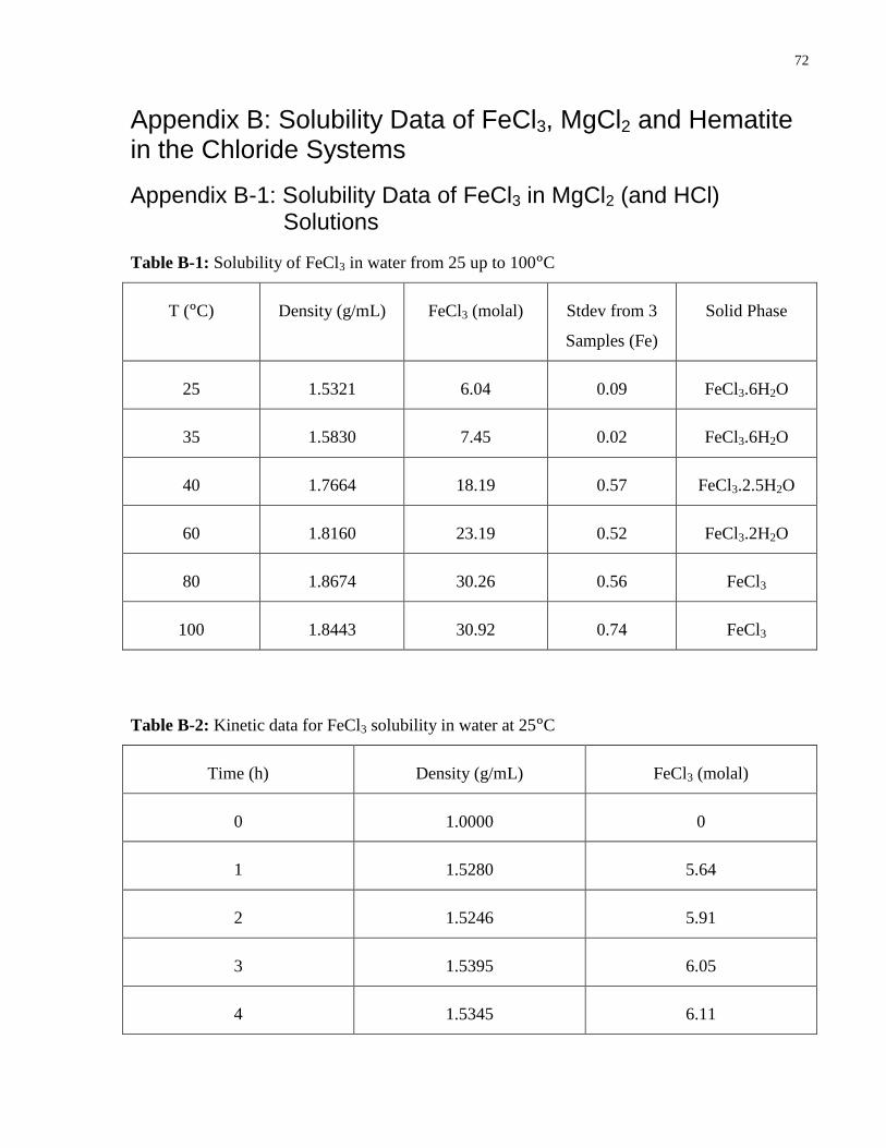
72
Appendix B: Solubility Data of FeCl3, MgCl2 and Hematite in the Chloride Systems
Appendix B-1: Solubility Data of FeCl3 in MgCl2 (and HCl) Solutions
Table B-1: Solubility of FeCl3 in water from 25 up to 100°C
T (°C) Density (g/mL) FeCl3 (molal) Stdev from 3
Samples (Fe)
Solid Phase
25 1.5321 6.04 0.09 FeCl3.6H2O
35 1.5830 7.45 0.02 FeCl3.6H2O
40 1.7664 18.19 0.57 FeCl3.2.5H2O
60 1.8160 23.19 0.52 FeCl3.2H2O
80 1.8674 30.26 0.56 FeCl3
100 1.8443 30.92 0.74 FeCl3
Table B-2: Kinetic data for FeCl3 solubility in water at 25°C
Time (h) Density (g/mL) FeCl3 (molal)
0 1.0000 0
1 1.5280 5.64
2 1.5246 5.91
3 1.5395 6.05
4 1.5345 6.11

73
5 1.5380 5.98
6 1.5255 6.08
8 1.5287 5.84
10 1.5282 5.82
12 1.5331 5.95
24 1.5313 6.14
Table B-3: Kinetic data for FeCl3 solubility in 6 molal MgCl2 solutions at 25°C
Time (h) Density (g/mL) MgCl2 (molal) FeCl3 (molal)
0 - 6 0
2 1.5384 3.71 6.44
3 1.5464 4.08 7.24
4 1.5455 3.95 7.24
5 1.5443 4.14 7.56
6 1.5392 3.94 7.43
8 1.5600 3.78 7.95
10 1.5678 3.50 7.62
12 1.5602 3.58 7.93
21 1.5666 3.55 7.87

74
24 1.5606 3.51 7.88
Table B-4: Kinetic data for FeCl3 solubility in water at 40°C
Time (h) Density (g/mL) FeCl3 (molal)
0 - 0
1.5 1.767 16.78
2.5 1.7442 17.32
6 1.7692 18.02
19.5 1.769 17.60
24 1.7617 18.62
Table B-5: Kinetic data for FeCl3 solubility in 1 molal MgCl2 solutions at 40°C
Time (h) Density (g/mL) MgCl2 (molal) FeCl3 (molal)
0 - 1 0
1 1.6830 1.08 13.84
4 1.7453 0.62 17.34
8 1.7585 0.66 17.26
12 1.7642 0.60 17.98
25 1.7675 0.53 17.75

75
Table B-6: Kinetic data for FeCl3 solubility in 3 molal MgCl2 solutions at 40°C
Time (h) Density (g/mL) MgCl2 (molal) FeCl3 (molal)
0 - 3 0
1 1.6508 2.57 13.80
4 1.7378 0.88 15.47
8 1.7417 0.84 16.56
12 1.7478 0.65 16.65
25 1.7559 0.55 17.32
Table B-7: Kinetic data for FeCl3 solubility in 5 molal MgCl2 solutions at 40°C
Time (h) Density (g/mL) MgCl2 (molal) FeCl3 (molal)
0 - 5 0
1.5 1.6234 4.52 12.81
2.5 1.6490 4.60 12.90
6 1.6351 4.53 12.97
19.5 1.6241 4.52 13.07
24 1.6440 4.42 13.02
Table B-8: Solubility data of FeCl3 in MgCl2 solutions from 25 up to 100°C
T (°C) Density MgCl2 FeCl3 Stdev from Stdev from Solid Phase

76
(g/mL) (molal) (molal) 3 Samples
(Mg)
3 Samples
(Fe)
25 1.5229 1.13 5.22 0.026 0.041 FeCl3.6H2O
25 1.5336 2.46 4.89 0.033 0.072 FeCl3.6H2O
25 1.5527 2.92 5.59 0.043 0.153 FeCl3.6H2O
25 1.5603 3.00 5.63 0.067 0.116 FeCl3.6H2O
25 1.5586 3.29 7.10 0.079 0.150 FeCl3.6H2O
25 1.5625 3.54 7.89 0.035 0.033 FeCl3.6H2O
25 1.7269 0.89 13.70 0.048 0.341 DS
25 1.6896 1.93 12.59 0.017 0.141 DS
25 1.6539 3.19 11.52 0.030 0.212 DS
25 1.6412 3.83 11.05 0.081 0.280 DS
35 1.5805 0.29 7.74 0.010 0.079 FeCl3.6H2O
35 1.5999 0.96 8.66 0.022 0.111 FeCl3.6H2O
35 1.5904 1.08 8.74 0.004 0.046 FeCl3.6H2O
40 1.7606 0.56 17.43 0.034 0.772 DS
40 1.7492 0.60 17.50 0.053 0.963 DS
40 1.7099 1.53 13.81 0.106 0.377 DS
40 1.6617 2.60 12.94 0.112 0.458 DS
40 1.6338 4.44 12.97 0.113 0.063 DS

77
60 1.8022 0.74 21.8 0.038 0.309 DS
60 1.7457 1.10 16.94 0.052 1.160 DS
60 1.6928 1.88 15.20 0.020 0.668 DS
60 1.6575 3.54 14.42 0.023 0.121 DS
80 1.8719 0.93 28.41 0.117 2.930 DS
80 1.7675 1.45 20.03 0.070 0.924 DS
80 1.6962 2.80 16.69 0.073 0.242 DS
80 1.6913 3.19 16.69 0.071 0.145 DS
100 1.8636 1.05 33.13 0.070 2.363 DS
100 1.7997 2.48 22.81 0.012 0.264 DS
100 1.7415 2.61 21.03 0.086 0.818 DS
100 1.6852 4.37 15.7 0.066 0.558 DS
Table B-9: Solubility data of FeCl3 in MgCl2 and HCl solutions from 25 up to 100°C
T (°C) Density
(g/mL)
HCl
(molal)
MgCl2
(molal)
FeCl3
(molal)
Stdev (3
samples)
HCl
Stdev (3
samples)
MgCl2
Stdev (3
samples)
FeCl3
Solid Phase
25 1.5527 0.63 2.65 5.94 0.014 0.032 0.051 FeCl3.6H2O
25 1.5481 1.05 2.35 5.99 0.013 0.047 0.063 FeCl3.6H2O
40 1.6709 0.86 2.33 12.87 0.053 0.045 0.544 DS

78
40 1.6398 1.22 3.56 11.93 0.039 0.153 0.508 DS
60 1.6763 0.79 3.38 14.25 0.032 0.086 0.461 DS
60 1.6507 1.30 3.63 13.85 0.0125 0.0274 0.0703 DS
100 1.6852 0.15 4.37 15.70 0.0107 0.0662 0.5579 DS
100 1.6963 0.43 3.99 16.24 0.0376 0.0536 0.1456 DS
Appendix B-2: Solubility Data of MgCl2 in FeCl3 Solutions
Table B-10: Solubility of MgCl2 in water from 25 up to 100°C
T (°C) Density (g/mL) MgCl2 (molal) Solid Phase
25 1.3031 5.79 MgCl2.6H2O
40 1.3048 6.05 MgCl2.6H2O
60 1.3200 6.32 MgCl2.6H2O
80 1.3319 6.80 MgCl2.6H2O
100 1.3463 7.61 MgCl2.6H2O
Table B-11: Kinetic data for MgCl2 solubility in water at 25°C
Time (h) Density (g/mL) MgCl2 (molal)
0 1.0000 0
1 1.3027 5.76

79
2 1.2991 5.81
3.5 1.3070 5.77
Table B-12: Kinetic data for MgCl2 solubility in 0.5 molal FeCl3 solutions at 25°C
Time (h) Density (g/mL) FeCl3 (molal) MgCl2 (molal)
0 - 1.384 0
0.5 1.3455 0.54 5.48
4 1.3319 0.55 5.55
6 1.3410 0.54 5.58
12 1.3439 0.54 5.66
25 1.3374 0.53 5.55
27.5 1.3486 0.53 5.48
Table B-13: Solubility data of MgCl2 in FeCl3 solutions from 25 up to 100°C
T (°C) Density (g/mL) FeCl3 (molal) MgCl2 (molal) Solid Phase
25 1.3430 0.53 5.52 MgCl2.6H2O
25 1.3732 1.09 5.22 MgCl2.6H2O
25 1.4016 1.71 5.03 MgCl2.6H2O
25 1.4402 2.38 4.8 MgCl2.6H2O

80
40 1.3381 0.49 5.81 MgCl2.6H2O
40 1.3657 0.98 5.53 MgCl2.6H2O
40 1.3994 1.51 5.36 MgCl2.6H2O
40 1.4228 2.10 5.32 MgCl2.6H2O
60 1.3414 0.43 6.23 MgCl2.6H2O
60 1.3665 0.85 6.09 MgCl2.6H2O
60 1.3757 1.29 5.96 MgCl2.6H2O
60 1.4013 1.77 5.94 MgCl2.6H2O
80 1.3503 0.36 6.66 MgCl2.6H2O
80 1.3677 0.7 6.65 MgCl2.6H2O
80 1.3680 1.06 6.59 MgCl2.6H2O
80 1.3865 1.46 6.54 MgCl2.6H2O
100 1.3661 0.25 7.36 MgCl2.6H2O
100 1.3714 0.49 7.4 MgCl2.6H2O
100 1.3650 0.74 7.37 MgCl2.6H2O
100 1.3836 1.01 7.35 MgCl2.6H2O
Appendix B-3: Solubility Data of Hematite in MgCl2 and HCl Solutions

81
Table B-14: Kinetic data for hematite solubility in 0.1 molal init. HCl at 60°C (measured)
Time (h) Density (g/mL) HCl Measured
(molal)
FeCl3 (molal)
0 0.9828 0.1001 0
0.33 0.9758 0.0946 0.00082
2 0.9724 0.0929 0.00157
5 0.9715 0.0909 0.00202
9.5 0.9817 0.0889 0.00247
22.5 0.9757 0.0874 0.00300
24 0.9758 0.0864 0.00304
26 0.9778 0.0862 0.00306
Table B-15: Kinetic data for hematite solubility in 0.1 molal init. HCl at 60°C (mass balance)
Time (h) Density (g/mL) HCl from Mass
Balance (molal)
FeCl3 (molal)
0 0.9828 0.1001 0
0.33 0.9758 0.0983 0.00082
2 0.9724 0.0965 0.00157
5 0.9715 0.0952 0.00203
9.5 0.9817 0.0928 0.00247
22.5 0.9757 0.0918 0.00300

82
24 0.9758 0.0917 0.00305
26 0.9778 0.0914 0.00306
Table B-16: Kinetic data for hematite solubility in 2.5 molal MgCl2 and 0.1 molal init. HCl at
60°C (measured)
Time (h) Density (g/mL) MgCl2 (molal) HCl Measured
(molal)
FeCl3 (molal)
0 1.138 2.46 0.1023 0
0.5 1.1449 2.49 0.0726 0.00678
2 1.1393 2.50 0.0403 0.01635
6 1.1361 2.47 0.0251 0.02155
12.5 1.1439 2.45 0.0173 0.02326
24.5 1.1384 2.46 0.0131 0.02394
Table B-17: Kinetic data for hematite solubility in 2.5 molal MgCl2 and 0.1 molal init. HCl at
60°C (mass balance)
Time (h) Density (g/mL) MgCl2 (molal) HCl from Mass
Balance (molal)
FeCl3 (molal)
0 1.138 2.46 0.1023 0
0.5 1.1449 2.49 0.0816 0.00678
2 1.1393 2.50 0.0534 0.01636

83
6 1.1361 2.47 0.0379 0.02156
12.5 1.1439 2.45 0.0319 0.02327
24.5 1.1384 2.46 0.0305 0.02396
Table B-18: Kinetic data for hematite solubility in 4 molal MgCl2 and 0.1 molal init. HCl at
60°C (measured)
Time (h) Density (g/mL) MgCl2 (molal) HCl Measured
(molal)
FeCl3 (molal)
0 1.2096 3.86 0.1020 0
0.5 1.2077 3.87 0.0068 0.02472
2 1.217 3.86 0.0034 0.02593
6 1.2219 3.84 0.0028 0.02692
12.5 1.2119 3.89 0.0017 0.02665
24.5 1.2199 3.85 0.0011 0.02641
Table B-19: Kinetic data for hematite solubility in 4 molal MgCl2 and 0.1 molal init. HCl at
60°C (mass balance)
Time (h) Density (g/mL) MgCl2 (molal) HCl from Mass
Balance (molal)
FeCl3 (molal)
0 1.2096 3.86 0.1020 0

84
0.5 1.2077 3.87 0.0281 0.02474
2 1.217 3.87 0.0237 0.02595
6 1.2219 3.85 0.0202 0.02693
12.5 1.2119 3.89 0.0221 0.02667
24.5 1.2199 3.85 0.0219 0.02643
Table B-20: Hematite Solubility in MgCl2 and HCl solutions at 60 and 90°C (measured)
T (°C) Init.
Density
(g/mL)
Init.
MgCl2
(molal)
Init. HCl
(molal)
Final
Density
(g/mL)
MgCl2
(molal)
HCl
Measured
(molal)
FeCl3
(molal)
60 0.9865 0 0.0997 0.9758 0 0.0864 0.0030
60 0.9912 0 0.2494 0.9873 0 0.1795 0.0198
60 0.9853 0 1.0320 0.9989 0 0.3328 0.2257
60 1.1444 2.49 0.1008 1.1428 2.47 0.0108 0.0247
60 1.1332 2.48 0.2560 1.1449 2.49 0.0142 0.0732
60 1.1484 2.50 1.0146 1.1735 2.48 0.0187 0.3174
60 1.2330 4.04 0.1014 1.2181 3.98 0.0040 0.0312
60 1.2298 4.08 0.2500 1.2301 4.08 0.0057 0.0797
60 1.2273 4.04 1.0077 1.2445 4.00 0.0063 0.3296
60 1.3010 6.34
(sat'd)
0.0942 1.3057 6.38
(sat'd)
0.0054 0.0270

85
60 1.3048 6.21
(sat'd)
0.2468 1.3148 6.33
(sat'd)
0.0038 0.0744
60 1.3080 6.02
(sat'd)
1.0184 1.3331 6.34
(sat'd)
0.0015 0.3039
90 0.9765 0 0.1007 0.9711 0 0.0878 0.0012
90 0.9711 0 0.2515 0.9784 0 0.1723 0.0179
90 0.9901 0 1.0138 1.0088 0 0.3442 0.2061
90 1.1470 2.47 0.1004 1.1440 2.50 0.0005 0.0132
90 1.1339 2.47 0.2568 1.1416 2.50 0.0044 0.0604
90 1.1472 2.48 1.0143 1.1696 2.50 0.0215 0.3070
90 1.2198 4.00 0.1022 1.2290 3.93 0 0.0171
90 1.2107 3.95 0.2564 1.2239 3.96 0 0.0657
90 1.2190 3.99 1.0156 1.2459 4.04 0.0029 0.3150
90 1.3324 7.07
(sat'd)
0.0613 1.3363 6.88
(sat'd)
0 0.0065
90 1.3383 6.93
(sat'd)
0.2150 1.3317 6.87
(sat'd)
0.0016 0.0517
90 1.3316 6.66
(sat'd)
0.6873 1.3452 6.65
(sat'd)
0.0031 0.2015

86
Table B-21: Hematite Solubility in MgCl2 and HCl solutions at 60 and 90°C (mass balance)
T (°C) Init.
Density
(g/mL)
Init.
MgCl2
(molal)
Init. HCl
(molal)
Final
Density
(g/mL)
MgCl2
(molal)
HCl from
Mass
Balance
(molal)
FeCl3
(molal)
60 0.9865 0 0.0997 0.9758 0 0.0919 0.0030
60 0.9912 0 0.2494 0.9873 0 0.1912 0.0198
60 0.9853 0 1.0320 0.9989 0 0.3520 0.2259
60 1.1444 2.49 0.1008 1.1428 2.48 0.0265 0.0247
60 1.1332 2.48 0.2560 1.1449 2.49 0.0348 0.0732
60 1.1484 2.50 1.0146 1.1735 2.49 0.0517 0.3178
60 1.2330 4.04 0.1014 1.2181 3.98 0.0085 0.0312
60 1.2298 4.08 0.2500 1.2301 4.00 0.0114 0.0798
60 1.2273 4.04 1.0077 1.2445 4.08 0.0147 0.3297
60 1.3010 6.34
(sat'd)
0.0942 1.3057 6.33
(sat'd)
0.0131 0.0270
60 1.3048 6.21
(sat'd)
0.2468 1.3148 6.36
(sat'd)
0.0240 0.0744
60 1.3080 6.02
(sat'd)
1.0184 1.3331 6.38
(sat'd)
0.1147 0.3052
90 0.9765 0 0.1007 0.9711 0 0.0977 0.0012
90 0.9711 0 0.2515 0.9784 0 0.1960 0.0179

87
90 0.9901 0 1.0138 1.0088 0 0.3859 0.2064
90 1.1470 2.47 0.1004 1.1440 2.50 0..0612 0.0133
90 1.1339 2.47 0.2568 1.1416 2.50 0.0748 0.0606
90 1.1472 2.48 1.0143 1.1696 2.51 0.0860 0.3077
90 1.2198 4.00 0.1022 1.2290 3.94 0.0496 0.0171
90 1.2107 3.95 0.2564 1.2239 3.97 0.0572 0.0658
90 1.2190 3.99 1.0156 1.2459 4.05 0.0625 0.3157
90 1.3324 7.07
(sat'd)
0.0613 1.3363 6.67
(sat'd)
0.0410 0.0065
90 1.3383 6.93
(sat'd)
0.2150 1.3317 6.89
(sat'd)
0.0605 0.0518
90 1.3316 6.66
(sat'd)
0.6873 1.3452 6.89
(sat'd)
0.0798 0.2021

88
Appendix C: XRD Patterns of The Equilibrating Solid Phases
Appendix C-1: XRD Patterns for FeCl3 Solubility Experiments
Figure C-1: XRD pattern for FeCl3 solubility in water at 25°C

89
Figure C-2: XRD pattern for Solubility of FeCl3 in 6 molal init. MgCl2 solutions at 25°C

90
Figure C-3: XRD pattern for FeCl3 solubility in water at 35°C
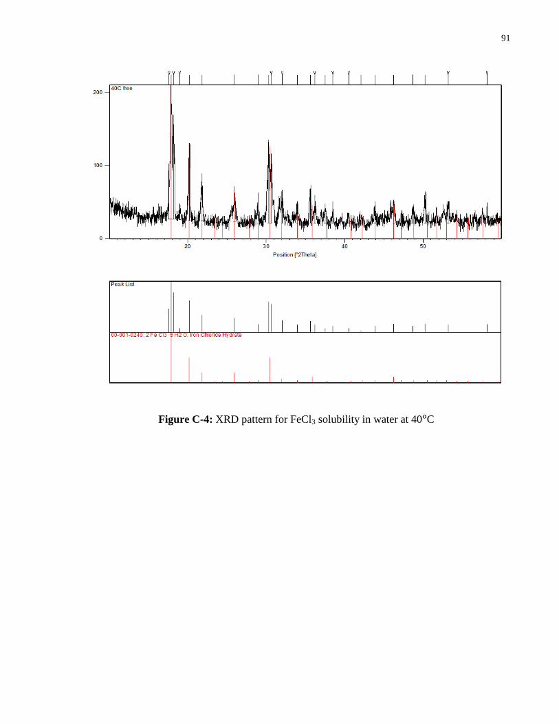
91
Figure C-4: XRD pattern for FeCl3 solubility in water at 40°C

92
Figure C-5: XRD pattern for FeCl3 solubility in 1 molal init. MgCl2 solutions at 40°C

93
Figure C-6: XRD pattern for FeCl3 solubility in 3 molal init. MgCl2 solutions at 40°C

94
Figure C-7: XRD pattern for FeCl3 solubility in 1 molal init. MgCl2 solutions at 60°C
Table C-1: XRD peak lists for FeCl3 solubility in 1 molal init. MgCl2 solutions at 60°C
Pos. [°2Th.] Height [cts] FWHM [°2Th.] d-spacing [Å] Rel. Int. [%]
12.7063 33.37 0.5510 6.96694 12.93
14.5881 258.17 0.1574 6.07221 100.00
14.7306 218.34 0.1181 6.01377 84.57
20.5652 210.53 0.0984 4.31890 81.55
24.2222 187.21 0.2755 3.67449 72.51
25.2573 55.50 0.1181 3.52620 21.50

95
31.7198 102.40 0.1181 2.82099 39.66
32.7218 95.37 0.2755 2.73686 36.94
35.8005 44.31 0.1181 2.50825 17.16
38.2206 38.26 0.1968 2.35481 14.82
41.8729 45.75 0.1574 2.15748 17.72
44.2576 29.34 0.2362 2.04661 11.36
47.0894 33.69 0.1968 1.92993 13.05
49.3051 13.82 0.6298 1.84826 5.35
53.2849 23.62 0.2362 1.71922 9.15
54.0951 27.57 0.1181 1.69537 10.68
55.9376 41.63 0.2362 1.64382 16.12
57.6879 6.83 0.5760 1.59672 2.65

96
Figure C-8: XRD pattern for FeCl3 solubility in 6 molal init. MgCl2 solutions at 60°C
Table C-2: XRD peak lists for FeCl3 solubility in 6 molal init. MgCl2 solutions at 60°C
Pos. [°2Th.] Height [cts] FWHM [°2Th.] d-spacing [Å] Rel. Int. [%]
12.9480 26.41 0.2362 6.83743 7.70
14.9053 342.83 0.1181 5.94367 100.00
20.9541 109.72 0.1574 4.23961 32.00
24.5530 76.45 0.2755 3.62573 22.30
25.6360 28.90 0.3936 3.47497 8.43
32.1054 99.89 0.1968 2.78799 29.14
33.1280 48.80 0.3149 2.70423 14.23
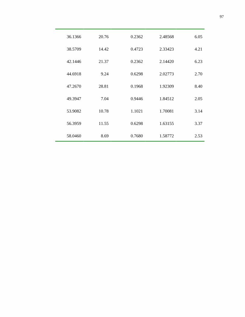
97
36.1366 20.76 0.2362 2.48568 6.05
38.5709 14.42 0.4723 2.33423 4.21
42.1446 21.37 0.2362 2.14420 6.23
44.6918 9.24 0.6298 2.02773 2.70
47.2670 28.81 0.1968 1.92309 8.40
49.3947 7.04 0.9446 1.84512 2.05
53.9082 10.78 1.1021 1.70081 3.14
56.3959 11.55 0.6298 1.63155 3.37
58.0460 8.69 0.7680 1.58772 2.53

98
Figure C-9: XRD pattern for FeCl3 solubility in 1 molal init. MgCl2 solutions at 80°C

99
Figure C-10: XRD pattern for FeCl3 solubility in 3 molal init. MgCl2 solutions at 80°C

100
Figure C-11: XRD pattern for FeCl3 solubility in 1 molal init. MgCl2 at 100°C
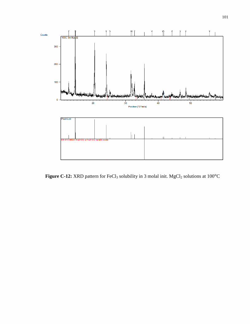
101
Figure C-12: XRD pattern for FeCl3 solubility in 3 molal init. MgCl2 solutions at 100°C

102
Appendix C-2: XRD Patterns for MgCl2 Solubility Experiments
Figure C-13: XRD pattern for MgCl2 solubility in 1.5 molal init. FeCl3 solutions at 25°C

103
Figure C-14: XRD pattern for MgCl2 solubility in 0.5 molal FeCl3 solutions at 80°C
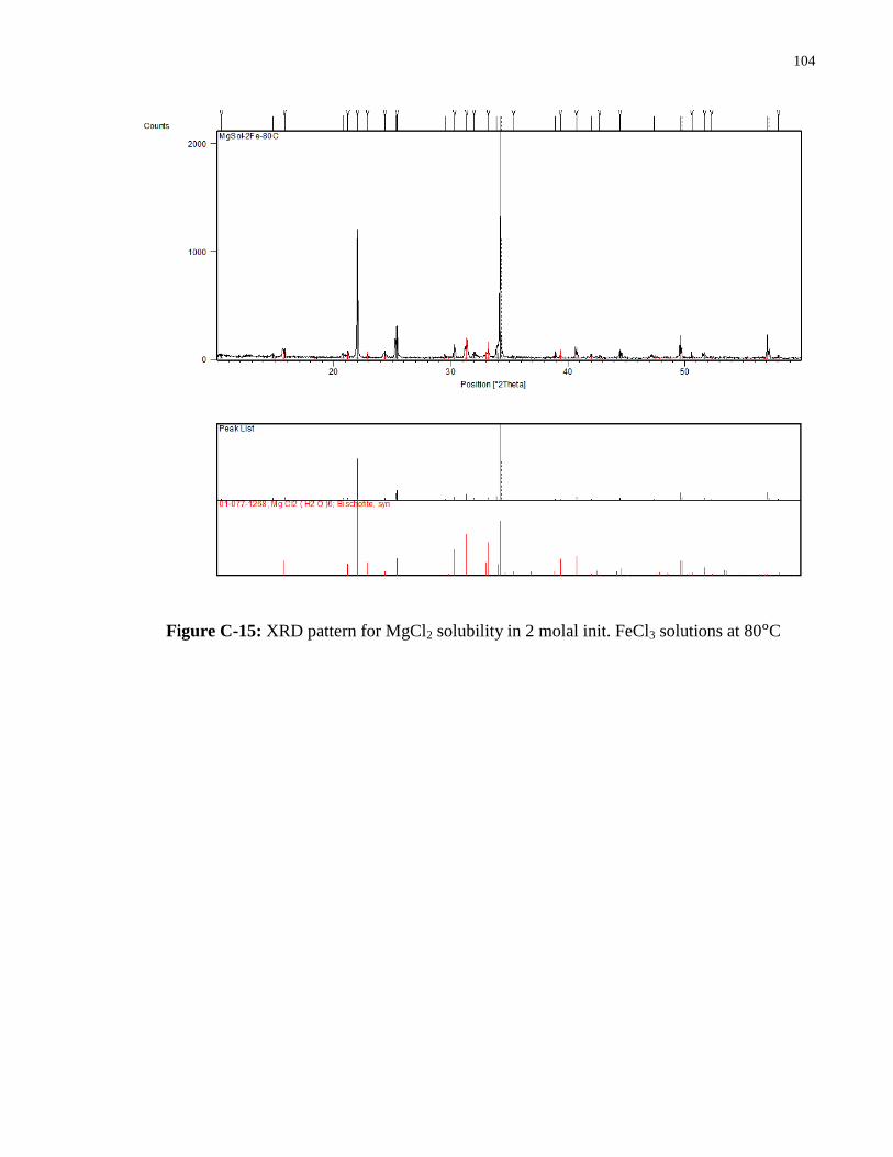
104
Figure C-15: XRD pattern for MgCl2 solubility in 2 molal init. FeCl3 solutions at 80°C

105
Figure C-16: XRD pattern for MgCl2 solubility in 0.5 molal FeCl3 solutions at 100°C

106
Figure C-17: XRD pattern for MgCl2 solubility in 1 molal FeCl3 solutions at 100°C

107
Appendix C-3: XRD Patterns for Hematite Experiments
Figure C-18: XRD pattern for hematite solubility in 0.1 molal HCl and 2.5 molal MgCl2 at 60°C
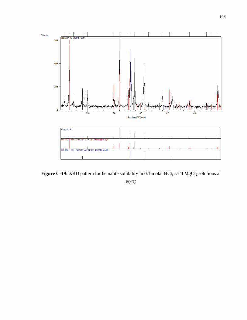
108
Figure C-19: XRD pattern for hematite solubility in 0.1 molal HCl, sat'd MgCl2 solutions at
60°C

109
Appendix D: Analysis of the Double Salt 2.5FeCl3.MgCl2.7.5H2O
Table D-1: Double salt 2.5FeCl3.MgCl2.7.5H2O chemical analysis
Condition Fe : Mg : Cl : H2O % Cl error
40°C, 1 molal
MgCl2 (1)
3.10 1 10.74 8.59 4.86
40°C, 1 molal
MgCl2 (2)
3.15 1 10.55 9.79 7.92
40°C, 3 molal
MgCl2 (1)
3.03 1 10.21 9.38 7.94
40°C, 3 molal
MgCl2 (2)
2.82 1 9.56 8.87 8.54
60°C, 1 molal
MgCl2 (1)
2.61 1 9.14 8.70 7.03
60°C, 3 molal
MgCl2 (1)
2.67 1 9.15 8.68 8.53
60°C, 3 molal
MgCl2 (2)
2.68 1 8.70 8.40 13.27
80°C, 3 molal
MgCl2 (1)
2.60 1 9.08 8.51 7.34
80°C, 3 molal
MgCl2 (2)
2.63 1 9.04 8.64 8.65
100°C, 3 2.67 1 9.20 9.16 8.22

110
molal MgCl2
(1)
100°C, 3
molal MgCl2
(2)
2.65 1 9.19 8.52 7.59
40°C, DS (1) 2.46 (EDTA) 1 (EDTA) 9.38 (MB) 7.59 0
40°C, DS (2) 2.54 (EDTA) 1 (EDTA) 9.50 (AgCl) 7.40 0.94
Note: Unless otherwise stated, metals analysis (Fe, Mg) were performed using ICP-OES and Cl
by chloride ISE. Crystalline water content was analyzed by mass balance.
EDTA: complexometric titration
MB: mass balance assuming all of metals (Fe and Mg) are in their chloride form
AgCl: Silver chloride precipitation (gravimetric method) for quantifying chloride content

111
Figure D-1: First TGA analysis of the double salt 2.5FeCl3.MgCl2.7.5H2O

112
Figure D-2: Second TGA analysis of the double salt 2.5FeCl3.MgCl2.7.5H2O

113
Appendix E: Validation Plots and Model Improvement for Fe(II)/Fe(III) Systems
Appendix E-1: FeSO4-H2O System
The solubility data for FeSO4 in water was taken from [9] for data up to 100°C and [10, 11] for
data above 100°C. OLI MSE default database predicts the solubility accurately from room
temperature up to 100°C, but above that temperature, OLI overestimates the solubility data.
Figure E-1: Default OLI MSE's simulated solubility of FeSO4 in water

114
Figure E-2: Improved OLI MSE's simulated FeSO4 solubility in water
Appendix E-2: FeSO4-H2SO4-H2O System
The literature data for the solubility of FeSO4 in H2SO4 solutions at elevated temperature was
taken from [9, 11, 12]. The default OLI MSE model complies with the literature data for up to
100°C. Above that temperature, due to inaccuracy of the model in predicting the solubility of
FeSO4 in water, OLI failed to represent the literature solubility data.

115
Figure E-3: Default OLI MSE's simulated FeSO4 solubility in H2SO4 solutions up to 100°C
Figure E-4: Improved OLI MSE's simulated FeSO4 solubility in H2SO4 solutions up to 100°C

116
Figure E-5: Default OLI MSE`s simulated FeSO4 solubility in H2SO4 solutions above 100°C
Figure E-6: Improved OLI MSE`s simulated FeSO4 solubility in H2SO4 solutions above 100°C

117
Appendix E-3: FeSO4-MgSO4-H2O System
The solubility data for FeSO4 in MgSO4 solutions was taken from [63]. The default OLI model
failed to accurately show the effect of MgSO4 addition on the solubility of FeSO4 at any
temperature studied.
Figure E-7: Default OLI MSE's simulated FeSO4 solubility in MgSO4 solutions

118
Figure E-8: Improved OLI MSE's simulated FeSO4 solubility in MgSO4 solutions
Appendix E-4: FeSO4-MgSO4-H2SO4-H2O System
The solubility data for this system was taken from [11]. The default OLI model overestimated
the literature data due to inaccuracy of the solubility prediction in binary FeSO4-H2O above
100°C.

119
Figure E-9: Default OLI MSE's simulated FeSO4 solubility in MgSO4 and H2SO4 solutions
Figure E-10: Improved OLI MSE's simulated FeSO4 solubility in MgSO4 and H2SO4 solutions

120
Appendix E-5: FeSO4-ZnSO4-H2SO4-H2O System
Solubility of FeSO4 in saturated ZnSO4 solutions at high temperatures was studied by [64, 65,
11]. It is obvious that the carry-over error from the solubility of binary FeSO4-H2O causes
overestimation of the solubility values in this system.
Figure E-11: Default OLI MSE's simulated FeSO4 solubility in ZnSO4 and H2SO4 solutions

121
Figure E-12: Improved OLI MSE's simulated FeSO4 solubility in ZnSO4 and H2SO4 solutions
Figure E-13: Default OLI MSE's simulated FeSO4 solubility in ZnSO4 and H2SO4 solutions at
200°C

122
Figure E-14: Improved OLI MSE's simulated FeSO4 solubility in ZnSO4 and H2SO4 solutions at
200°C
Appendix E-6: FeCl2-H2O System
The default OLI model reproduces the solubility data for FeCl2-H2O system up to 120°C taken
from [9, 66, 67, 68]

123
Figure E-15: Default OLI MSE's simulated FeCl2 solubility in water
Appendix E-7: FeCl2-HCl-H2O System
The solubility data for FeCl2 in HCl solutions was taken from [9, 69, 70]. The default OLI MSE
model is in a good agreement with the literature data up to 100°C. However, due to improve the
performance of FeSO4-H2SO4-H2O, minor changes is needed for shared interaction parameter
Fe2+
- H3O+. This change improves the performance of the model for this system, especially at
100°C.

124
Figure E-16: Default OLI MSE's simulated FeCl2 solubility in HCl solutions
Figure E-17: Improved OLI MSE's simulated FeCl2 solubility in HCl solutions

125
Appendix E-8: FeCl2-MgCl2 System
The solubility of FeCl2 in MgCl2 solutions was studied by [71, 72, 73, 57]. OLI MSE prediction
is consistent with the literature data up to 3 molal MgCl2 solutions and above that, OLI
underestimates the literature solubility data. Furthermore, at 70°C, OLI predicted the presence
of FeCl2.2H2O solid phase which was not seen in the literature data. The double salt
FeCl2.MgCl2.8H2O which was present up to 70°C has not been implemented in the default OLI
MSE database.
Figure E-18: Default OLI MSE's simulated FeCl2 solubility in MgCl2 solutions

126
Figure E-19: Improved OLI MSE's simulated FeCl2 solubility in MgCl2 solutions
Appendix E-9: FeCl2-MgCl2-HCl-H2O System
The solubility data was taken from [74]. It is apparent that OLI underestimated the solubility at
elevated MgCl2 concentration due to the same error seen in the binary FeCl2-MgCl2 system.
However, the effect of acid addition which reduces the solubility was correctly shown in the
default model.

127
Figure E-20: Default OLI MSE's simulated FeCl2 solubility in MgCl2 and HCl solutions
Figure E-21: Improved OLI MSE's simulated FeCl2 solubility in MgCl2 and HCl solutions

128
Appendix E-10: Fe2O3-H2SO4-H2O System
Solubility of hematite in sulfuric acid solutions above 100°C was previously studied by [75, 76,
77] but their results were inaccurate due to sampling errors during solubility measurement. More
recently, Reid and Papangelakis re-performed the solubility experiment by addressing all the
sampling errors from previous studies [78]. For this study, only the literature data provided by
Reid and Papangelakis was used. The default OLI MSE database underestimates the solubility
data at any temperature studied.
Figure E-22: Default OLI MSE's simulated Fe2O3 solubility in H2SO4 solutions at 130-170°C

129
Figure E-23: Improved OLI MSE's simulated Fe2O3 solubility in H2SO4 solutions at 130-170°C
Figure E-24: Default OLI MSE's simulated Fe2O3 solubility in H2SO4 solutions at 230-270°C

130
Figure E-25: Improved OLI MSE's simulated Fe2O3 solubility in H2SO4 solutions at 230-270°C
Appendix E-11: Fe2O3-MgSO4-H2SO4-H2O System
The solubility data provided by [78] was used to validate the OLI MSE default model. Due to
underestimation of the solubility of hematite in Fe2O3-H2SO4-H2O system, the errors are carried
over to this quaternary system.

131
Figure E-26: Default OLI MSE's simulated Fe2O3 solubility in MgSO4 and H2SO4 solutions
Figure E-27: Improved OLI MSE's simulated Fe2O3 solubility in MgSO4 and H2SO4 solutions

132
Appendix E-12: NaFe3(SO4)2(OH)6-H2SO4 System
The solubility data was provided by [79] but the default OLI MSE database does not have
sodium jarosite as the default species, thus no OLI simulation could be performed.
Figure E-28: Default OLI MSE's simulated Na-jarosite solubility in H2SO4 solutions

133
Figure E-29: Improved OLI MSE's simulated Na-jarosite solubility in H2SO4 solutions

134
Appendix F: Lists of Regressed OLI Parameters
Table F-1: Default OLI MSE standard state parameters for solid and aqueous species
Species ΔGof (cal/mol) S
o (cal/mol.K) ΔH
of (cal/mol)
FeSO4.7H2O (s) -598064.1 80.16869 -723891
FeSO4.H2O (s) -256326.5 8.65124 -303812.1
FeSO4 (aq) -199444.1 -5.70945 -234599.9
Fe2O3 (s) -175367.6 15.46522 -196566
Table F-2: Regressed standard state parameters of solid and aqueous species
Species ΔGof
(cal/mol)
So
(cal/mol.K)
ΔHof
(cal/mol)
Other Parameters
FeSO4.7H2O (s) -598439.5 123.1721 -711444.1
FeSO4.H2O (s) -257112.1 38.52326 -295691
FeSO4 (aq) -197086.7 54.0136 -214436
Fe2O3 (s) -178267.4 6.183049 -202234
FeSO4+ (aq) -184680 -31.07075 -222705.5 HA1 = 7.6754
HA2 = -24503
HA3 = -696.62
HA4 = 2.6326E+06

135
HC1 = -0.28386
HC2 = 288120
HW = 385280
Fe(SO4)2- (aq) -369152.9 -15.55063 -443403 HC1 = 69.82967
Fe2(SO4)3 (aq) -537220.4 28.03979 -627275.3 HC1 = 170.9113
NaFe3(SO4)2(OH)6 (s) -779067.7 147.3791 -879385 Cp = 616.39 + 0.09121T
- 20376000/T2
Table F-3: Default OLI MSE mid-range binary interaction parameters between ions/aqueous
species
Binary Interaction BMD CMD
Fe2+
- SO42-
BMD0 = 5.720929
BMD1 = -0.02804112
BMD2 = 1179.33
Fe2+
- HSO4- BMD0 = -33.56567
Fe2+
- H3O+ BMD0 = -14.41686
BMD1 = 0.04981539
Mg2+
- HSO4- BMD0 = 19.9975
BMD2 = -6542.72
CMD2 = -9262.47
Fe3+
- H3O+ BMD2 = -665.362

136
FeOH2+
- HSO4- BMD2 = -6000
Table F-4: Regressed mid-range binary interaction parameters between ions/aqueous species
Binary Interaction BMD CMD
Fe2+
- SO42-
BMD0 = 4967.292
BMD1 = -7.854654
BMD2 = -807851.6
CMD0 = -5326.328
CMD1 = 8.973077
CMD2 = 833187.2
Fe2+
- HSO4- BMD0 = -91.83042
BMD1 = 0.2012855
Fe2+
- H3O+ BMD0 = 118.347
BMD1 = -0.181243
BMD2 = -18886.5
Fe2+
- Mg2+
BMD0 = 43.17417
BMD1 = -0.06165801
BMD2 = -4991.604
Fe2+
- Zn2+
BMD0 = -638.8605
BMD1 = 1.36925
Mg2+
- HSO4- BMD0 = 6.953257
BMD1 = -0.001238579
Fe3+
- H3O+ BMD0 = -39.92635

137
BMD1 = -0.1768866
BMD2 = -10920
FeOH2+
- HSO4- BMD0 = 226.0031
BMD1 = -5.6340103E-2
BMD2 =-61722.12
FeOH2+
- H3O+ BMD0 = 210.5307
BMD1 = -0.3667933
BMD2 = 15460.15
Fe(SO4)2- - HSO4
- BMD0 = -2.598352
BMD1 = -0.4128314
BMD2 = 119172.1
Fe(SO4)2- - H3O
+ BMD0 = 18.71168
BMD1 = -0.4223134
BMD2 = 58631.09
Fe3+
- Na+ BMD0 = 240.6021
BMD1 = -0.9782702
BMD2 = 271251.9
Fe(SO4)2- - Na
+ BMD0 = 116.9141
BMD1 = 0.3929999
BMD2 = 1932.883

138