CHEMICAL METHODS FOR INTERSTITIAL WATERANALYSIS ABOARD JOIDES RESOLUTION

OCEAN DRILLING PROGRAMTEXAS A&M UNIVERSITY

Technical Note 15

Joris M. GieskesMarine Research Division, A-015

Scripps Institution of OceanographyUniversity of California, San Diego

La Jolla, California 92093U.S.A.

Toshitaka GamoOcean Research Institute

University of Tokyo1-15-1 Minamidai, Nakano-ku

Tokyo 164Japan

Hans BrumsackGeochemistry InstituteUniversity of GöttingenGoldschmidtstrasse 1

D-3400 GöttingenFederal Republic of Germany

August 1991

2

TABLE OF CONTENTSIntroduction 3

Units 4

Standards 5

Chloride 8

Calcium 10

Magnesium 13

PmH 15

Alkalinity 19

Sulfate 24

Boron 34

Iodide 36

Bromide 38

Ammonium 40

Silica 42

Phosphate 46

Nitrite 48

Nitrate 49

Atomic Absorption methods 52

References 59

3

INTRODUCTION

Methodologies in the chemistry laboratory aboard JOIDES Resolution have undergone an

increasing degree of sophistication during the last few years. During Leg 102 Gieskes and

Peretsman (1986) reported on the procedures of the chemistry laboratory at that time. Here we

wish to update that 1986 "cookbook" with each method presented in its own section. A copy of

this technical note is kept onboard ship in loose-leaf-folder fashion to facilitate continuous

updating of methods. We recommend this stapled copy be taken to the ship, with any new

procedural techniques being noted, so analyses could be repeated in your laboratory following

the cruise.

In addition to the already described methodologies (Gieskes and Peretsman, 1986), this

manual also contains a discussion of atomic absorption (AA) methods. For this purpose use has

been made of the notes on this subject originated by Hans Brumsack during ODP Leg 127.

We are appreciative of the assistance given to us by Valerie Clark and Scott Chaffey.

They helped with questions and worked with us especially on AA and pH methodologies.

In a separate manual, "Wet Chemical Analysis of Sediments for Major Element

Composition on JOIDES Resolution" by Joris Gieskes and Toshitaka Gamo, wet chemical

methods for the analysis of major constituents of sedimentary rocks are described. That

methodology, though perhaps somewhat less accurate than XRF methodology, can serve as an

alternate, especially during any potential down times of the XRF. "Cookbooks" for other

specialized methodologies are also kept aboard ship and at ODP headquarters. Requests for

information regarding methodologies not described in this technical note may be directed to the

Manager of Science Operations, Ocean Drilling Program, 1000 Discovery Drive, College

Station, TX 77845-9547, U.S.A.

4

UNITS

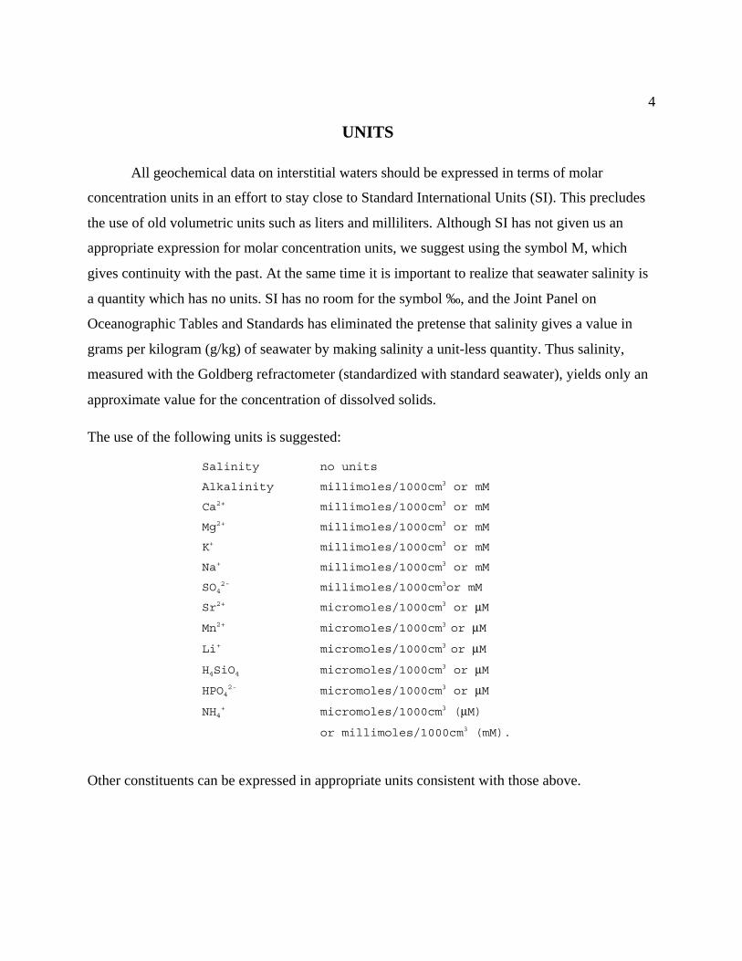
All geochemical data on interstitial waters should be expressed in terms of molar

concentration units in an effort to stay close to Standard International Units (SI). This precludes

the use of old volumetric units such as liters and milliliters. Although SI has not given us an

appropriate expression for molar concentration units, we suggest using the symbol M, which

gives continuity with the past. At the same time it is important to realize that seawater salinity is

a quantity which has no units. SI has no room for the symbol ‰, and the Joint Panel on

Oceanographic Tables and Standards has eliminated the pretense that salinity gives a value in

grams per kilogram (g/kg) of seawater by making salinity a unit-less quantity. Thus salinity,

measured with the Goldberg refractometer (standardized with standard seawater), yields only an

approximate value for the concentration of dissolved solids.

The use of the following units is suggested:

Salinity no units

Alkalinity millimoles/1000cm3 or mM

Ca2+ millimoles/1000cm3 or mM

Mg2+ millimoles/1000cm3 or mM

K+ millimoles/1000cm3 or mM

Na+ millimoles/1000cm3 or mM

SO42- millimoles/1000cm3or mM

Sr2+ micromoles/1000cm3 or µM

Mn2+ micromoles/1000cm3 or µM

Li+ micromoles/1000cm3 or µM

H4SiO4 micromoles/1000cm3 or µM

HPO42- micromoles/1000cm3 or µM

NH4+ micromoles/1000cm3 (µM)

or millimoles/1000cm3 (mM).

Other constituents can be expressed in appropriate units consistent with those above.

5

STANDARDS

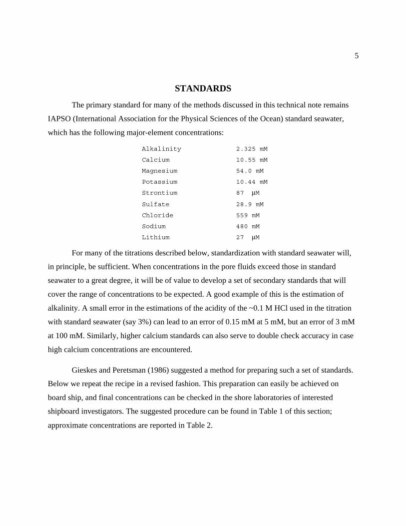
The primary standard for many of the methods discussed in this technical note remains

IAPSO (International Association for the Physical Sciences of the Ocean) standard seawater,

which has the following major-element concentrations:

Alkalinity 2.325 mM

Calcium 10.55 mM

Magnesium 54.0 mM

Potassium 10.44 mM

Strontium 87 µM

Sulfate 28.9 mM

Chloride 559 mM

Sodium 480 mM

Lithium 27 µM

For many of the titrations described below, standardization with standard seawater will,

in principle, be sufficient. When concentrations in the pore fluids exceed those in standard

seawater to a great degree, it will be of value to develop a set of secondary standards that will

cover the range of concentrations to be expected. A good example of this is the estimation of

alkalinity. A small error in the estimations of the acidity of the ~0.1 M HCl used in the titration

with standard seawater (say 3%) can lead to an error of 0.15 mM at 5 mM, but an error of 3 mM

at 100 mM. Similarly, higher calcium standards can also serve to double check accuracy in case

high calcium concentrations are encountered.

Gieskes and Peretsman (1986) suggested a method for preparing such a set of standards.

Below we repeat the recipe in a revised fashion. This preparation can easily be achieved on

board ship, and final concentrations can be checked in the shore laboratories of interested

shipboard investigators. The suggested procedure can be found in Table 1 of this section;

approximate concentrations are reported in Table 2.

6

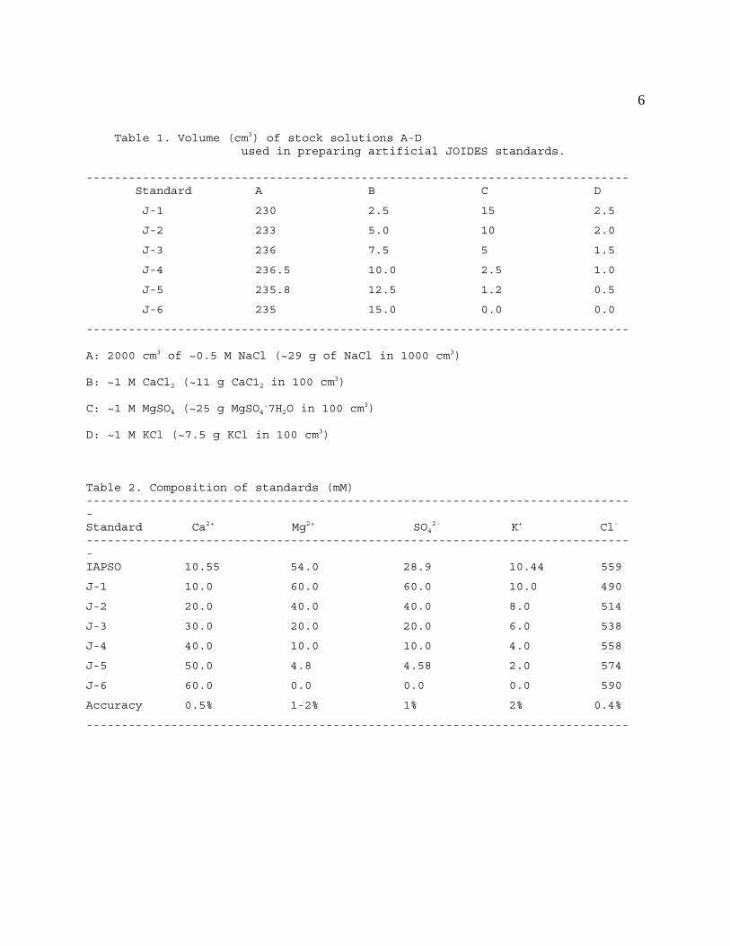
Table 1. Volume (cm3) of stock solutions A-D used in preparing artificial JOIDES standards.

----------------------------------------------------------------------------- Standard A B C D

J-1 230 2.5 15 2.5

J-2 233 5.0 10 2.0

J-3 236 7.5 5 1.5

J-4 236.5 10.0 2.5 1.0

J-5 235.8 12.5 1.2 0.5

J-6 235 15.0 0.0 0.0

-----------------------------------------------------------------------------

A: 2000 cm3 of ~0.5 M NaCl (~29 g of NaCl in 1000 cm3)

B: ~1 M CaCl2 (~11 g CaC12 in 100 cm3)

C: ~1 M MgSO4 (~25 g MgSO4.7H2O in 100 cm

3)

D: ~1 M KCl (~7.5 g KCl in 100 cm3)

Table 2. Composition of standards (mM)------------------------------------------------------------------------------Standard Ca2+ Mg2+ SO4

2- K+ Cl-

------------------------------------------------------------------------------IAPSO 10.55 54.0 28.9 10.44 559

J-1 10.0 60.0 60.0 10.0 490

J-2 20.0 40.0 40.0 8.0 514

J-3 30.0 20.0 20.0 6.0 538

J-4 40.0 10.0 10.0 4.0 558

J-5 50.0 4.8 4.58 2.0 574

J-6 60.0 0.0 0.0 0.0 590

Accuracy 0.5% 1-2% 1% 2% 0.4%

-----------------------------------------------------------------------------

7

For Ca and Mg, the standards can be checked by using the "super Ca-Mg method"

described in the section on calcium.

Standards are calculated on the basis of precise molarities from the previous page. They

will change if amounts in Table 1 are slightly different; hence they require double checking in

shore-based laboratories.

For the other constituents, again it is important to adopt standards that bracket the range

of concentrations to be expected, which, especially for silica, phosphate, and ammonium, can

constitute a considerable range. In this manner, even if considerable dilutions will be necessary,

the samples and standards will go through a similar treatment.

8

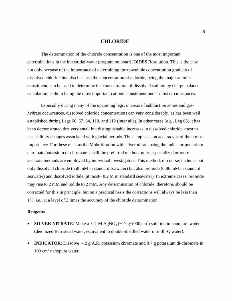
CHLORIDE

The determination of the chloride concentration is one of the most important

determinations in the interstitial-water program on board JOIDES Resolution. This is the case

not only because of the importance of determining the downhole concentration gradient of

dissolved chloride but also because the concentration of chloride, being the major anionic

constituent, can be used to determine the concentration of dissolved sodium by charge balance

calculation, sodium being the most important cationic constituent under most circumstances.

Especially during many of the upcoming legs, in areas of subduction zones and gas-

hydrate occurrences, dissolved chloride concentrations can vary considerably, as has been well

established during Legs 66, 67, 84, 110, and 112 (inter alia). In other cases (e.g., Leg 86) it has

been demonstrated that very small but distinguishable increases in dissolved chloride attest to

past salinity changes associated with glacial periods. Thus emphasis on accuracy is of the utmost

importance. For these reasons the Mohr titration with silver nitrate using the indicator potassium

chromate/potassium di-chromate is still the preferred method, unless specialized or more

accurate methods are employed by individual investigators. This method, of course, includes not

only dissolved chloride (558 mM in standard seawater) but also bromide (0.86 mM in standard

seawater) and dissolved iodide (at most~ 0.2 M in standard seawater). In extreme cases, bromide

may rise to 2 mM and iodide to 2 mM. Any determination of chloride, therefore, should be

corrected for this in principle, but on a practical basis the corrections will always be less than

1%, i.e., at a level of 2 times the accuracy of the chloride determination.

Reagents

• SILVER NITRATE: Make a 0.1 M AgNO3 (~17 g/1000 cm3) solution in nanopure water

(deionized Barnstead water, equivalent to double-distilled water or milli-Q water).

• INDICATOR: Dissolve 4.2 g A.R. potassium chromate and 0.7 g potassium di-chromate in

100 cm3 nanopure water.

9

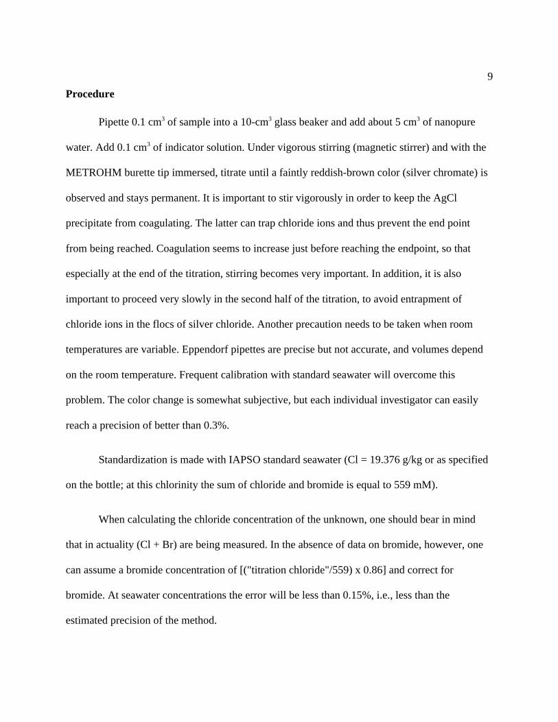
Procedure

Pipette 0.1 cm3 of sample into a 10-cm3 glass beaker and add about 5 cm3 of nanopure

water. Add 0.1 cm3 of indicator solution. Under vigorous stirring (magnetic stirrer) and with the

METROHM burette tip immersed, titrate until a faintly reddish-brown color (silver chromate) is

observed and stays permanent. It is important to stir vigorously in order to keep the AgCl

precipitate from coagulating. The latter can trap chloride ions and thus prevent the end point

from being reached. Coagulation seems to increase just before reaching the endpoint, so that

especially at the end of the titration, stirring becomes very important. In addition, it is also

important to proceed very slowly in the second half of the titration, to avoid entrapment of

chloride ions in the flocs of silver chloride. Another precaution needs to be taken when room

temperatures are variable. Eppendorf pipettes are precise but not accurate, and volumes depend

on the room temperature. Frequent calibration with standard seawater will overcome this

problem. The color change is somewhat subjective, but each individual investigator can easily

reach a precision of better than 0.3%.

Standardization is made with IAPSO standard seawater (Cl = 19.376 g/kg or as specified

on the bottle; at this chlorinity the sum of chloride and bromide is equal to 559 mM).

When calculating the chloride concentration of the unknown, one should bear in mind

that in actuality (Cl + Br) are being measured. In the absence of data on bromide, however, one

can assume a bromide concentration of [("titration chloride"/559) x 0.86] and correct for

bromide. At seawater concentrations the error will be less than 0.15%, i.e., less than the

estimated precision of the method.

10

CALCIUM

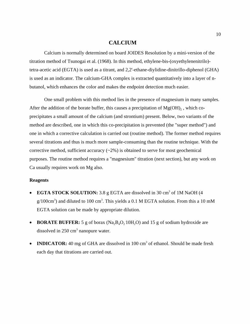
Calcium is normally determined on board JOIDES Resolution by a mini-version of the

titration method of Tsunogai et al. (1968). In this method, ethylene-bis-(oxyethylenenitrilo)-

tetra-acetic acid (EGTA) is used as a titrant, and 2,2'-ethane-diylidine-dinitrillo-diphenol (GHA)

is used as an indicator. The calcium-GHA complex is extracted quantitatively into a layer of n-

butanol, which enhances the color and makes the endpoint detection much easier.

One small problem with this method lies in the presence of magnesium in many samples.

After the addition of the borate buffer, this causes a precipitation of Mg(OH)2 , which co-

precipitates a small amount of the calcium (and strontium) present. Below, two variants of the

method are described, one in which this co-precipitation is prevented (the "super method") and

one in which a corrective calculation is carried out (routine method). The former method requires

several titrations and thus is much more sample-consuming than the routine technique. With the

corrective method, sufficient accuracy (~2%) is obtained to serve for most geochemical

purposes. The routine method requires a "magnesium" titration (next section), but any work on

Ca usually requires work on Mg also.

Reagents

• EGTA STOCK SOLUTION: 3.8 g EGTA are dissolved in 30 cm3 of 1M NaOH (4

g/100cm3) and diluted to 100 cm3. This yields a 0.1 M EGTA solution. From this a 10 mM

EGTA solution can be made by appropriate dilution.

• BORATE BUFFER: 5 g of borax (Na2B4O2.10H2O) and 15 g of sodium hydroxide are

dissolved in 250 cm3 nanopure water.

• INDICATOR: 40 mg of GHA are dissolved in 100 cm3 of ethanol. Should be made fresh

each day that titrations are carried out.

11

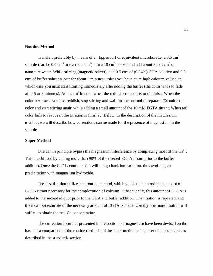
Routine Method

Transfer, preferably by means of an Eppendorf or equivalent microburette, a 0.5 cm3

sample (can be 0.4 cm3 or even 0.2 cm3) into a 10 cm3 beaker and add about 2 to 3 cm3 of

nanopure water. While stirring (magnetic stirrer), add 0.5 cm3 of (0.04%) GHA solution and 0.5

cm3 of buffer solution. Stir for about 3 minutes, unless you have quite high calcium values, in

which case you must start titrating immediately after adding the buffer (the color tends to fade

after 5 or 6 minutes). Add 2 cm3 butanol when the reddish color starts to diminish. When the

color becomes even less reddish, stop stirring and wait for the butanol to separate. Examine the

color and start stirring again while adding a small amount of the 10 mM EGTA titrant. When red

color fails to reappear, the titration is finished. Below, in the description of the magnesium

method, we will describe how corrections can be made for the presence of magnesium in the

sample.

Super Method

One can in principle bypass the magnesium interference by complexing most of the Ca2+.

This is achieved by adding more than 98% of the needed EGTA titrant prior to the buffer

addition. Once the Ca2+ is complexed it will not go back into solution, thus avoiding co-

precipitation with magnesium hydroxide.

The first titration utilizes the routine method, which yields the approximate amount of

EGTA titrant necessary for the complexation of calcium. Subsequently, this amount of EGTA is

added to the second aliquot prior to the GHA and buffer addition. The titration is repeated, and

the next best estimate of the necessary amount of EGTA is made. Usually one more titration will

suffice to obtain the real Ca concentration.

The correction formulas presented in the section on magnesium have been devised on the

basis of a comparison of the routine method and the super method using a set of substandards as

described in the standards section.

12

Standardization

Standardization is achieved by titration of IAPSO standard seawater. It should, however,

be remembered that standardization of the routine method should use the same procedure as the

routine method, and the super method should use the super procedure.

Corrections for strontium usually are trivial and can be ignored for most practical purposes. For

calcium concentration close to seawater, there is no real problem because standardization

includes the IAPSO strontium.

13

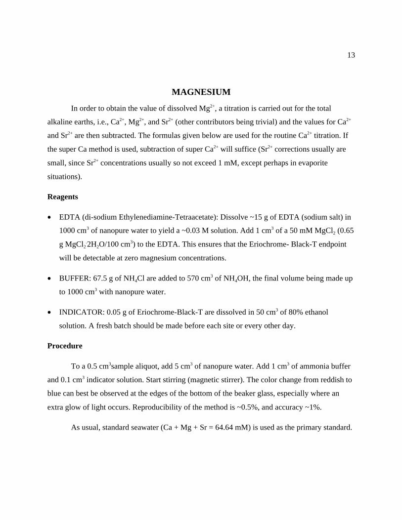
MAGNESIUM

In order to obtain the value of dissolved Mg2+, a titration is carried out for the total

alkaline earths, i.e., Ca2+, Mg2+, and Sr2+ (other contributors being trivial) and the values for Ca2+

and Sr2+ are then subtracted. The formulas given below are used for the routine Ca2+ titration. If

the super Ca method is used, subtraction of super Ca2+ will suffice (Sr2+ corrections usually are

small, since Sr2+ concentrations usually so not exceed 1 mM, except perhaps in evaporite

situations).

Reagents

• EDTA (di-sodium Ethylenediamine-Tetraacetate): Dissolve ~15 g of EDTA (sodium salt) in

1000 cm3 of nanopure water to yield a ~0.03 M solution. Add 1 cm3 of a 50 mM MgCl2 (0.65

g MgCl2.2H2O/100 cm3) to the EDTA. This ensures that the Eriochrome- Black-T endpoint

will be detectable at zero magnesium concentrations.

• BUFFER: 67.5 g of NH4Cl are added to 570 cm3 of NH4OH, the final volume being made up

to 1000 cm3 with nanopure water.

• INDICATOR: 0.05 g of Eriochrome-Black-T are dissolved in 50 cm3 of 80% ethanol

solution. A fresh batch should be made before each site or every other day.

Procedure

To a 0.5 cm3sample aliquot, add 5 cm3 of nanopure water. Add 1 cm3 of ammonia buffer

and 0.1 cm3 indicator solution. Start stirring (magnetic stirrer). The color change from reddish to

blue can best be observed at the edges of the bottom of the beaker glass, especially where an

extra glow of light occurs. Reproducibility of the method is ~0.5%, and accuracy ~1%.

As usual, standard seawater (Ca + Mg + Sr = 64.64 mM) is used as the primary standard.

14

Calculations

As mentioned in the previous section, the routine method for calcium requires a

correction for interference by magnesium. Gieskes and Peretsman (1986) suggested two simple

formulas for the calculation of Ca2+ and Mg2+, following the procedure of Gieskes and Lawrence

(1976). In part, these formulas are based on titrations carried out on the standards described in

the standards section.

Denoting total alkaline earths by Dt and the "routine" calcium titration value by Cat, we obtain

the corrected Mg and Ca values as follows:

Mgcorr = (Dt – 0.94Cat)/1.01;

Cacorr = 0.94Cat + 0.01Mgcorr.

Eventually, when data are available on dissolved Sr2+, minor corrections can be made for this

component, as follows:

Cafinal = Cacorr – 0.8Sr + 0.08;

Mgfinal = Mgcorr + 0.2Sr.

However, as pointed out before, this correction is usually superfluous. Furthermore, seawater

strontium is usually taken into the calcium titration standardization through the use of standard

seawater.

15

pmH

For the pH measurement, the standard operation has been based on the use of the NBS

(National Bureau of Standards) buffers. These buffers are designed as low ionic strength

solutions made of potassium hydrogen phthalate (pH = 4.008 at 25o C), mixtures of mono-

hydrogen and di-hydrogen phosphates (pH = 6.865 and 7.413 at 25o C, respectively), and 0.01 m

borax (pH = 9.18 at 25o C). One problem with these buffers has always been that they have given

the impression to the casual user that the thermodynamic activity of the hydrogen ion is actually

being measured in any solution, independent of what the ionic strength might be. Bates and

Culberson (1977) point out the fallacy of this concept, especially in marine systems. For these

reasons a subcommittee of the Joint Panel on Tables and Standards (JPOTS) has advocated the

adoption of a new pH scale, utilizing buffers designed specifically for media of ionic strengths

similar to that of seawater.

The newly proposed pH scale relies on the determination of the "free" hydrogen ion

concentration scale (Bates and Culberson, 1977), in which mH is the concentration of the

free hydrogen ions in mol/kg-H2O and where we denote -logmH with the symbol pmH.

For the purpose of standardizing pH electrode systems in terms of this new pH scale,

Bates and Culberson (1977), Khoo et al. (1977), and Bates and Calais (1981) developed two

buffers, which have been specifically designed for use in seawater and seawater-like solutions.

These buffers are described in Table 1.

It should be noted that Bates and Calais (1981) propose the use of a specially prepared

artificial seawater, taking great care in the preparation of the NaCl. During Leg 131 we did not

have pure NaCl available, and for this reason we made the buffer solutions from Nankai Trough

bottom water (S = 34.68), which has an approximate alkalinity of 2.5 mM, i.e., considerably less

than that introduced in the preparation of the buffer. Thus we consider the effect of the small

bicarbonate contribution to be small enough to be neglected. Surface water will be equally

useful.

16

In order to study the effects of salinity and of the composition of artificial seawater,

BIS and TRIS buffer solutions were also made in Nankai Trough bottom seawater diluted to S =

30, as well as in artificial seawater with 476, 558, 637 mM NaCl and 47.8, 55.9, 63.1 mM

MgSO4. The latter solutions were prepared as artificial seawater "equivalents" for salinities 30,

35, and 40. Results are reported in Table 2. From this table it is apparent that the solution

chemical effects are not large and that pmH values can be obtained with a precision of better

than 0.02 pmH units.

Standardization with pH buffers based on the NBS scale yielded an electrode slope of

57.64 mV/pH unit. Our solutions with TRIS/BIS on the other hand yielded a slope of 59.38

mV/pmH unit. The latter slope is much closer to the theoretical value of 59.15 mV/pmH unit.

A comparison with NBS standard (pH = 7.413), using a slope of 59.15 mV/pH unit,

yielded a systematic difference between the two pH scales of 0.114 + 0.013, pmH values being

systematically lower. This is mostly the result of the difference in concept: the pmH scale is a

concentration scale whereas the NBS scale yields activities, with an albeit ill-defined activity

coefficient.

We recommend the adoption of the TRIS/BIS standards with the caution that the values

should be reported as pmH, not pH. The occasional user may think that a tremendous change has

been made, but what really has happened is that the pH measurements are now based on a more

honest concept of concentration, rather than on a so-called thermodynamic entity.

The additional advantage, of course, is that the alkalinity electrodes will not further

undergo the shock treatment of large salinity changes during calibration, as they will remain

always in solutions of ionic strengths similar to those of seawater.

New standards for pmH

Two new standards are recommended for use in pmH measurements on board JOIDES

Resolution: TRIS and BIS standards and their hydrochlorides:

17

• TRIS = tris(hydroxymethyl)amino methane or (2-amino-2-(hydroxymethyl)-

1,3-propanediol).

• BIS = bis(hydroxymethyl)methylamino methane or (2-amino-2-methyl-1,3-

propanediol).

Tris, Tris.HCl, and Bis are obtainable commercially (e.g., from Sigma Chemical Co., St.

Louis, MO 63178). Bis.HCl is not commercially available because of the very hygroscopic

nature of Bis.HCl. Bis.HCl must be crystallized from a concentrated solution of Bis that has been

neutralized with purified HCl. This is produced by heating deionized water in a glass beaker then

adding Bis while stirring. When the solution becomes saturated (precipitation is observed) add

HCl (Seastar brand in the Teflon bottle in acid cabinet) until neutral (pH 7 tested with pH paper).

Cool solution (a gel will form at the bottom) then decant water. Place in a warm oven until dried

(it will form a smooth surface and need to be scraped from the container). Remove the chemical

immediately to a vaccuum desiccator to cool. This chemical must be kept in a desiccator and

weighed quickly (take first weight) when making up the buffer. It should be redried in the oven

then cooled in the desiccator each time prior to weighing.

Bates and Calais (1981) propose a special recipe for artificial seawater. We found,

however, that Nankai Trough bottom water (S = 34.89) suffices for this purpose. Surface water

will be equally useful.

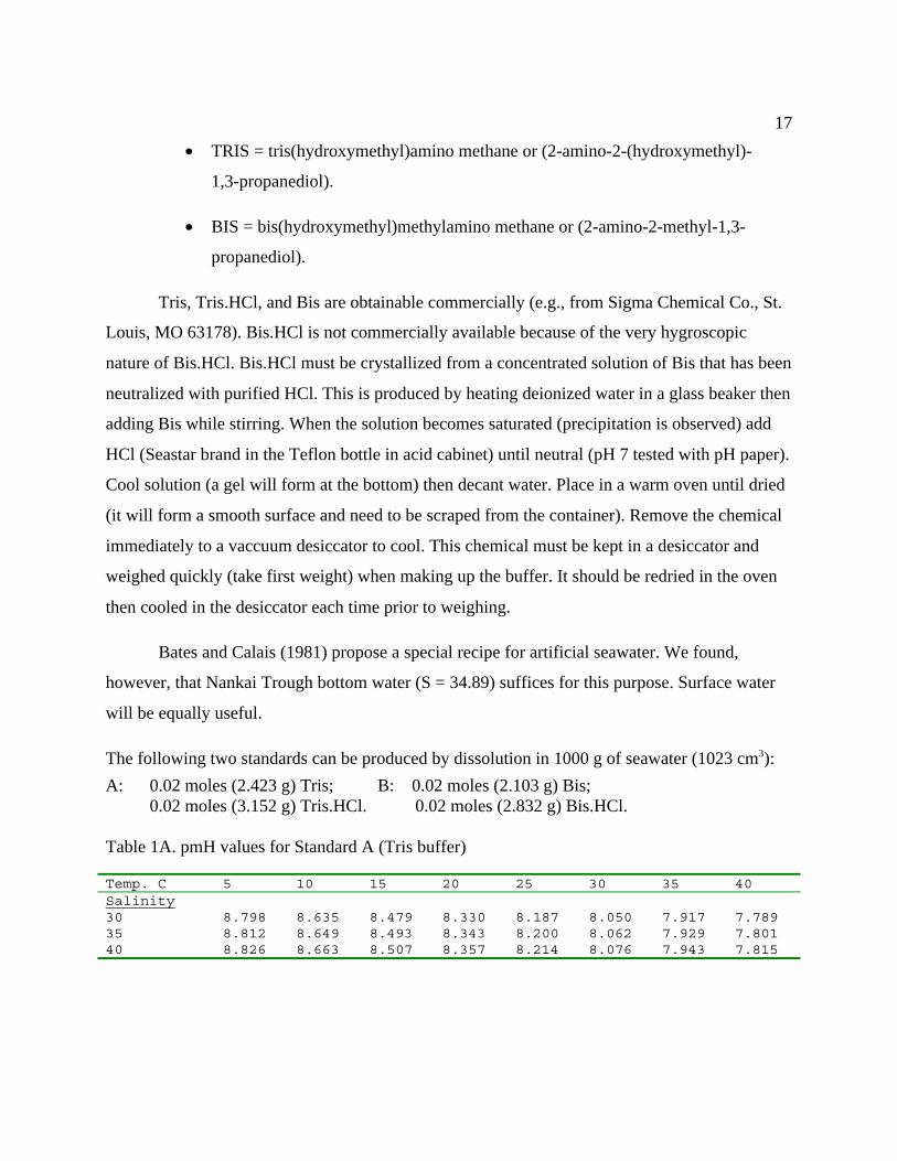
The following two standards can be produced by dissolution in 1000 g of seawater (1023 cm3):

A: 0.02 moles (2.423 g) Tris; B: 0.02 moles (2.103 g) Bis; 0.02 moles (3.152 g) Tris.HCl. 0.02 moles (2.832 g) Bis.HCl.

Table 1A. pmH values for Standard A (Tris buffer)

Temp. C 5 10 15 20 25 30 35 40Salinity30 8.798 8.635 8.479 8.330 8.187 8.050 7.917 7.78935 8.812 8.649 8.493 8.343 8.200 8.062 7.929 7.80140 8.826 8.663 8.507 8.357 8.214 8.076 7.943 7.815

18

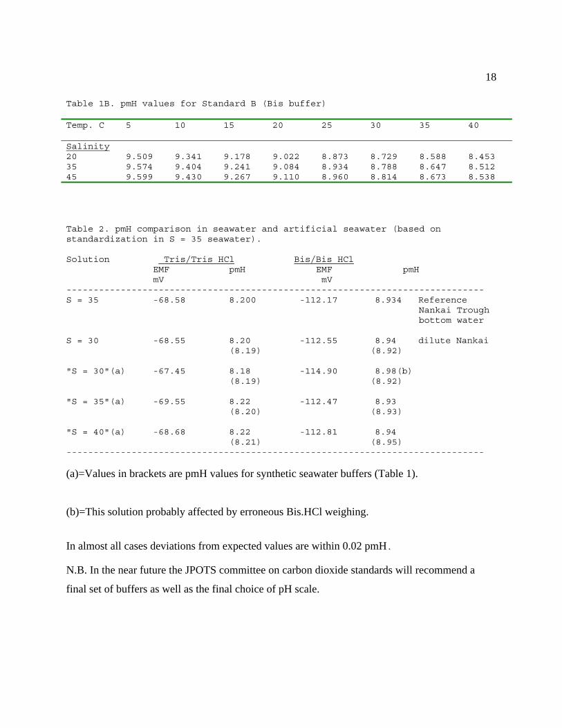
Table 1B. pmH values for Standard B (Bis buffer)

Temp. C

5 10 15 20 25 30 35 40

Salinity20 9.509 9.341 9.178 9.022 8.873 8.729 8.588 8.45335 9.574 9.404 9.241 9.084 8.934 8.788 8.647 8.51245 9.599 9.430 9.267 9.110 8.960 8.814 8.673 8.538

Table 2. pmH comparison in seawater and artificial seawater (based onstandardization in S = 35 seawater).

Solution Tris/Tris HCl Bis/Bis HCl EMF pmH EMF pmH mV mV-----------------------------------------------------------------------------S = 35 -68.58 8.200 -112.17 8.934 Reference

Nankai Troughbottom water

S = 30 -68.55 8.20 -112.55 8.94 dilute Nankai (8.19) (8.92)

"S = 30"(a) -67.45 8.18 -114.90 8.98(b) (8.19) (8.92)

"S = 35"(a) -69.55 8.22 -112.47 8.93 (8.20) (8.93)

"S = 40"(a) -68.68 8.22 -112.81 8.94 (8.21) (8.95)-----------------------------------------------------------------------------

(a)=Values in brackets are pmH values for synthetic seawater buffers (Table 1).

(b)=This solution probably affected by erroneous Bis.HCl weighing.

In almost all cases deviations from expected values are within 0.02 pmH.

N.B. In the near future the JPOTS committee on carbon dioxide standards will recommend a

final set of buffers as well as the final choice of pH scale.

19

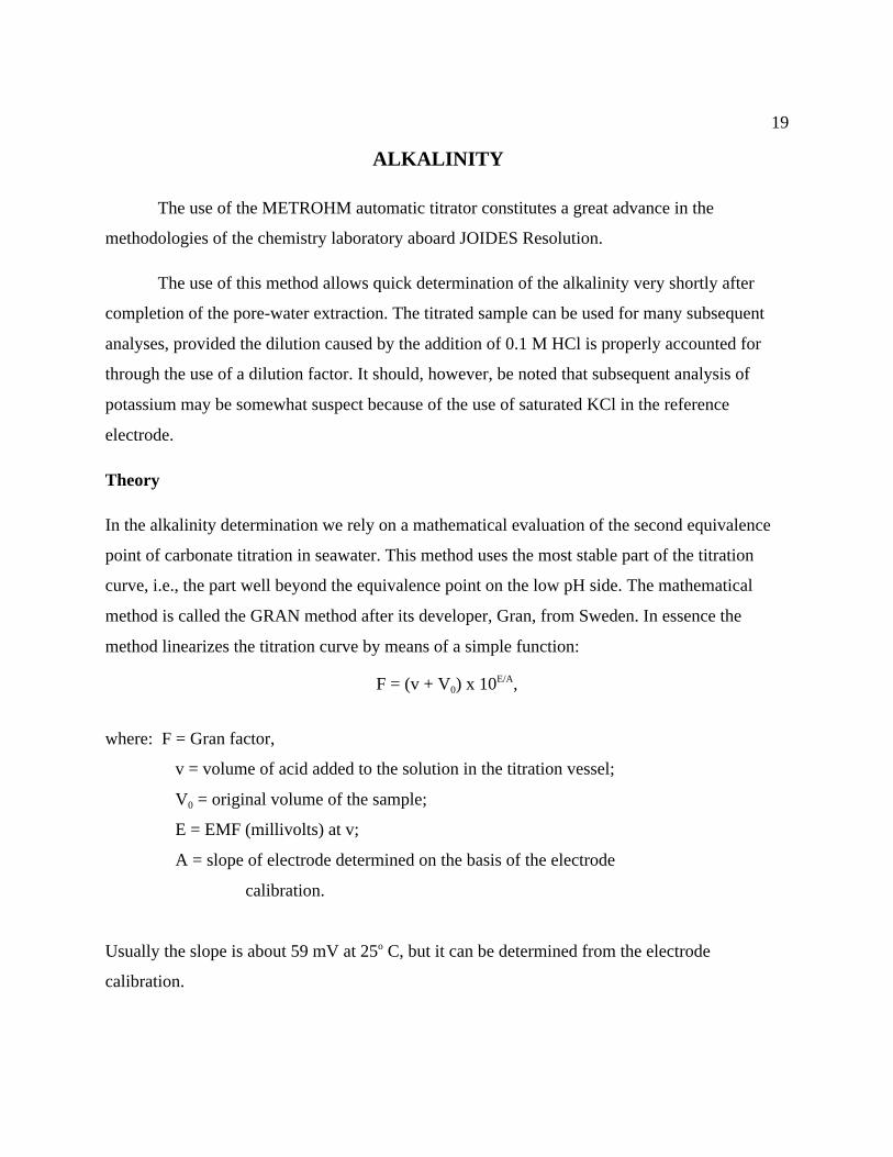
ALKALINITY

The use of the METROHM automatic titrator constitutes a great advance in the

methodologies of the chemistry laboratory aboard JOIDES Resolution.

The use of this method allows quick determination of the alkalinity very shortly after

completion of the pore-water extraction. The titrated sample can be used for many subsequent

analyses, provided the dilution caused by the addition of 0.1 M HCl is properly accounted for

through the use of a dilution factor. It should, however, be noted that subsequent analysis of

potassium may be somewhat suspect because of the use of saturated KCl in the reference

electrode.

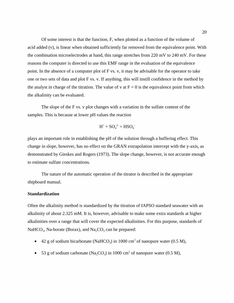
Theory

In the alkalinity determination we rely on a mathematical evaluation of the second equivalence

point of carbonate titration in seawater. This method uses the most stable part of the titration

curve, i.e., the part well beyond the equivalence point on the low pH side. The mathematical

method is called the GRAN method after its developer, Gran, from Sweden. In essence the

method linearizes the titration curve by means of a simple function:

F = (v + V0) x 10E/A,

where: F = Gran factor,

v = volume of acid added to the solution in the titration vessel;

V0 = original volume of the sample;

E = EMF (millivolts) at v;

A = slope of electrode determined on the basis of the electrode

calibration.

Usually the slope is about 59 mV at 25o C, but it can be determined from the electrode

calibration.

20

Of some interest is that the function, F, when plotted as a function of the volume of

acid added (v), is linear when obtained sufficiently far removed from the equivalence point. With

the combination microelectrodes at hand, this range stretches from 220 mV to 240 mV. For these

reasons the computer is directed to use this EMF range in the evaluation of the equivalence

point. In the absence of a computer plot of F vs. v, it may be advisable for the operator to take

one or two sets of data and plot F vs. v. If anything, this will instill confidence in the method by

the analyst in charge of the titration. The value of v at F = 0 is the equivalence point from which

the alkalinity can be evaluated.

The slope of the F vs. v plot changes with a variation in the sulfate content of the

samples. This is because at lower pH values the reaction

H+ + SO42- = HSO4

-

plays an important role in establishing the pH of the solution through a buffering effect. This

change in slope, however, has no effect on the GRAN extrapolation intercept with the y-axis, as

demonstrated by Gieskes and Rogers (1973). The slope change, however, is not accurate enough

to estimate sulfate concentrations.

The nature of the automatic operation of the titrator is described in the appropriate

shipboard manual.

Standardization

Often the alkalinity method is standardized by the titration of IAPSO standard seawater with an

alkalinity of about 2.325 mM. It is, however, advisable to make some extra standards at higher

alkalinities over a range that will cover the expected alkalinities. For this purpose, standards of

NaHCO3, Na-borate (Borax), and Na2CO3 can be prepared:

• 42 g of sodium bicarbonate (NaHCO3) in 1000 cm3 of nanopure water (0.5 M),

• 53 g of sodium carbonate (Na2CO3) in 1000 cm3 of nanopure water (0.5 M),

21

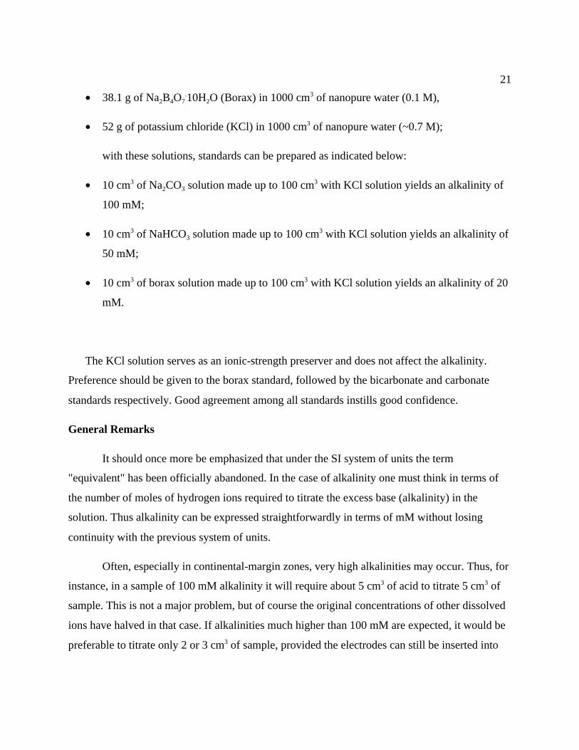
• 38.1 g of Na2B4O7.10H2O (Borax) in 1000 cm3 of nanopure water (0.1 M),

• 52 g of potassium chloride (KCl) in 1000 cm3 of nanopure water (~0.7 M);

with these solutions, standards can be prepared as indicated below:

• 10 cm3 of Na2CO3 solution made up to 100 cm3 with KCl solution yields an alkalinity of

100 mM;

• 10 cm3 of NaHCO3 solution made up to 100 cm3 with KCl solution yields an alkalinity of

50 mM;

• 10 cm3 of borax solution made up to 100 cm3 with KCl solution yields an alkalinity of 20

mM.

The KCl solution serves as an ionic-strength preserver and does not affect the alkalinity.

Preference should be given to the borax standard, followed by the bicarbonate and carbonate

standards respectively. Good agreement among all standards instills good confidence.

General Remarks

It should once more be emphasized that under the SI system of units the term

"equivalent" has been officially abandoned. In the case of alkalinity one must think in terms of

the number of moles of hydrogen ions required to titrate the excess base (alkalinity) in the

solution. Thus alkalinity can be expressed straightforwardly in terms of mM without losing

continuity with the previous system of units.

Often, especially in continental-margin zones, very high alkalinities may occur. Thus, for

instance, in a sample of 100 mM alkalinity it will require about 5 cm3 of acid to titrate 5 cm3 of

sample. This is not a major problem, but of course the original concentrations of other dissolved

ions have halved in that case. If alkalinities much higher than 100 mM are expected, it would be

preferable to titrate only 2 or 3 cm3 of sample, provided the electrodes can still be inserted into

22

the solution.

Under all circumstances the total volume of acid added to the sample aliquot

(record the size of the aliquot also) must be recorded on the storage vial so that future

workers on the sample are alerted to the dilution factor to be used in the calculation of original

concentrations.

Note that for the HCl, use must be made of ultrapure HCl. Normal (reagent grade) 0.1

M HCl can have a significant amount of iodide (~100-300 µM) in it, which can easily be avoided

by using triple distilled ultrapure HCl.

It is of great importance to calibrate the 5 cm3 and 3 cm3 pipettes with distilled water

and to note their precise volumes. The volumes should remain fixed for the duration of the

cruise. They are important for establishing the dilution factor to be used for further work on the

samples. The standardization of the acid, of course, takes account of the volumes.

Note on Alkalinity Calibration (by J. Gieskes)

Until now calibration of the alkalinity has relied on calibration with IAPSO standard

seawater. I think it is time to eliminate this and to proceed with a calibration based on a 40 mM

(alkalinity) borax solution. The procedure for preparation is described in the "Standardization"

section of this chapter, but it is worth repeating here:

1. Make a ~0.7 M KCl solution: 52 g KCl in 1000 cm3 of nanopure water.

2. Make a solution of 38.1 g of Na2B4O7.10H2O in 1000 cm3 nanopure water (0.1 M).

3. Take 20 cm3 of borax solution (2) and dilute to a total volume of 100 cm3 with the KCl

solution. The KCl serves to make the solution of approximately the same ionic strength

as seawater (in this case an ionic strength of about 0.56 M; seawater has an ionic strength

of ~0.7 M). The alkalinity of this solution is 40 mM.

With the 5 cm3 sampling pipette, transfer 5 cm3 of this borate standard solution into the

23

titration vessel. Titrate and evaluate the alkalinity with the presently available program

(omitting the IAPSO correction-factor step). This titration will yield an alkalinity that is probably

not quite equal to 40 mM, for the following reasons:

(a) The volume of the pipette is not quite equal to 5 cm3, and

(b) the acid molarity of the 0.1 M HCl solution is not quite equal to 0.1 M.

Now, from the estimated alkalinity and the actual alkalinity, calculate a calibration factor

that goes in the program, much like the previous factor that adjusted for the IAPSO "alkalinity."

In a way, that factor also adjusted for the difference in volume, although this fact was not known.

Of course this necessitates the creation of different correction factors for a 3 cm3 or a 10 cm3

sample because of differences in true volumes. For these reasons I suggest the following

program modifications:

1. Make the program easily accessible to the input of the calibration factor.

2. At the beginning of the cruise, calibrate with three different-sized pipettes, say of 3, 5,

and 10 cm3. The volumes of these pipettes should not be changed from then on (tape

them up). Work out the calibration factors for each of the pipettes and put them into the

program in conjunction with the volume size command now used.

3. Make some extra standards of different alkalinities over the range of interest to serve as a

double check. Weighing these standards presented no problems on the ship, and we

obtained very good results during Leg 131.

24

SULFATE

Determination of dissolved sulfate in interstitial waters recovered from a drill hole is

important for assessing diagenetic processes involving the alteration of organic matter and also

for analyzing the overall quality of the database. Because of the anionic nature of the sulfate ion,

it is not affected directly by ion exchange processes and thus is more independent of artifacts

created by the extrusion of pore fluids at other than in situ conditions. Any spurious deviations

from an overall trend with depth can be interpreted in terms of potential contamination with

surface seawater that is pumped down the hole during the drilling process. Naturally this method

works best when sulfate concentrations are zero, in which case any small increase can be directly

attributable to contamination.

Determination of sulfate is routinely carried out by means of the DIONEX ion

chromatograph, which uses a small amount of sample and provides very reproducible results.

However, if a quick semiquantitative estimate of dissolved sulfate is needed an alternate method

can be used which involves the precipitation of sulfate in an excess of BaCl2. A comparison of

the degree of cloudiness can be used as a qualitative estimate. Stabilization of the suspension

with glycerol can, in principle, be used for a semiquantitative estimate of dissolved sulfate (see

below).

Dionex Method

The ion chromatographic method has the advantage that measurements can be made on

very small quantities of sample. Typically, the standard representative of seawater concentration

and the samples are made of 0.25 cm3 of standard/sample solution diluted with nanopure water to

50 cm3 (representing a final concentration of ~145 µM for IAPSO standard seawater). If less

sample is available, smaller amounts can be prepared with the same dilution.

The operation of the DIONEX ion chromatograph is discussed in detail in the operations

manual on board ship. In this section only a brief description of the method is presented.

25

Principle of the Method

This method is based on an ion exchange process between a mobile phase and exchange

groups covalently bound to a stationary matrix. Upon introduction into the system, the sample is

carried by a mobile phase that holds the counter ions to different degrees, dependant on the

bonding strength between the cation/anion and the exchange group of the matrix. Because the

method of cation exchange (for Ca2+, Mg2+, K+, and Li+) chromatography is somewhat

cumbersome and time consuming in nature and also because faster, equally acceptable methods

are available on board JOIDES Resolution, the only ion exchange chromatographic method

routinely used is the anionic exchange method, which allows the determination of SO42- and

potentially also of Br-.

Although each individual user of the DIONEX system should consult the operations

manual in detail, it may be useful to reiterate the principle of operation. Details of the theory can

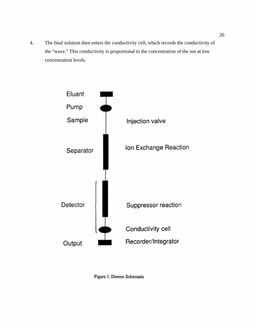
be found in Weiss (1986). Figure 1 (from Weiss, 1986) shows the following flow diagram:

1. The mobile phase is pumped through the system by means of a double reciprocating

pump that allows for a pulse-free flow.

2. The sample is introduced through a loop injector and swept to the column by the mobile

phase (the eluant) in which the ion exchange reactions separate the various anions (Cl-,

Br-, SO42-) into separate waves, which then arrive at the detector as the sodium salts (the

eluant consists of Na2CO3/NaHCO3).

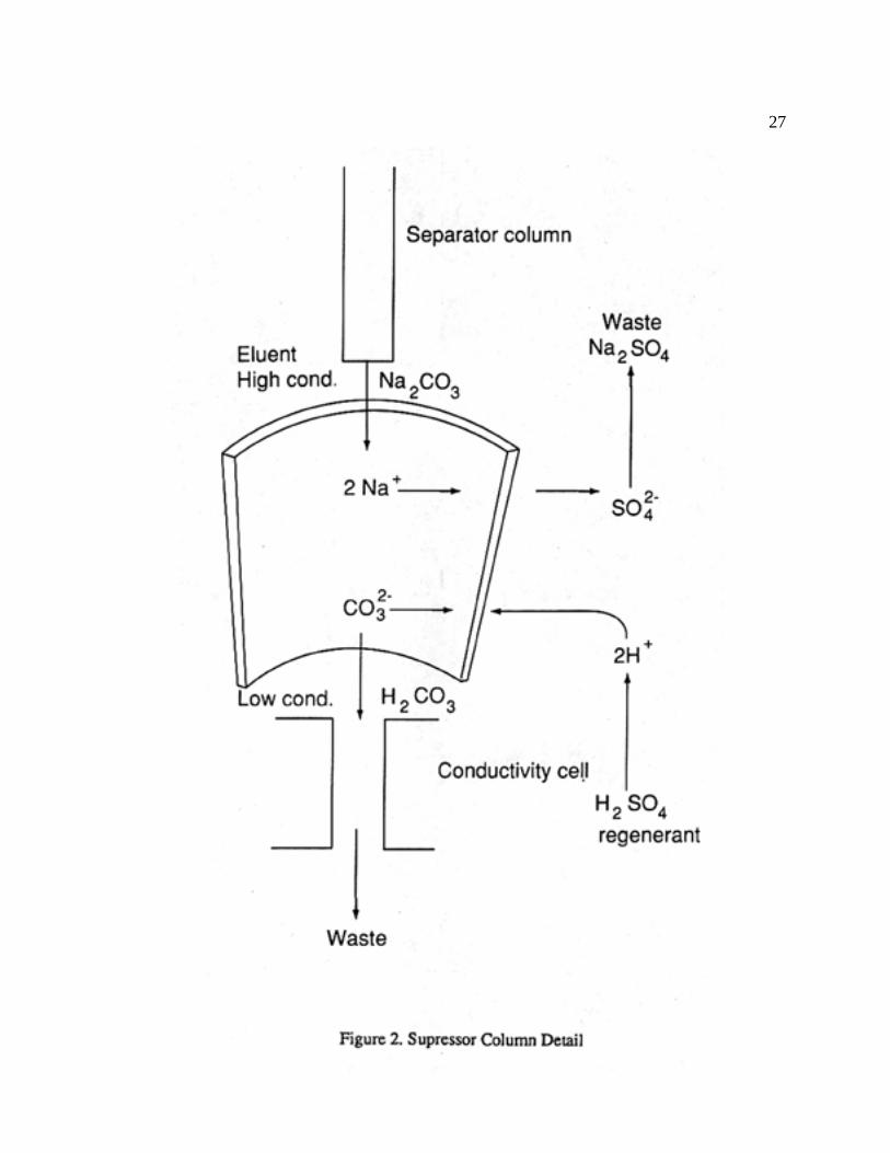
3. The first part of the detector system (Fig. 2) consists of the suppressor, which consists of

a semipermeable membrane. The solution from the separator column runs through the

interior of the membrane fiber, whereas a dilute acid (H2SO4) runs countercurrently in

contact with the exterior of the membrane. This allows H+ ions to be exchanged across

the semipermeable membrane in exchange for Na+ ions. This, in turn, converts the greater

conducting HCO3- and CO3

2- ions into less conducting H2CO3, and the less conducting

sodium salts of Cl-, Br-, and SO42- are converted into their greater conducting acids.

26

4. The final solution then enters the conductivity cell, which records the conductivity of

the "wave." This conductivity is proportional to the concentration of the ion at low

concentration levels.

27

28

Reagents

• ELUANT: 0.0022 M Na2CO3 ( 0.933 g in 4000 cm3); 0.0028 M NaHCO3 (add 0.941 g to

above solution); pH = 10.23.

• REGENERANT: 0.025 M H2SO4 (1.4 cm3 concentrated H2SO4 in 2000 cm3 nanopure

water).

Standards

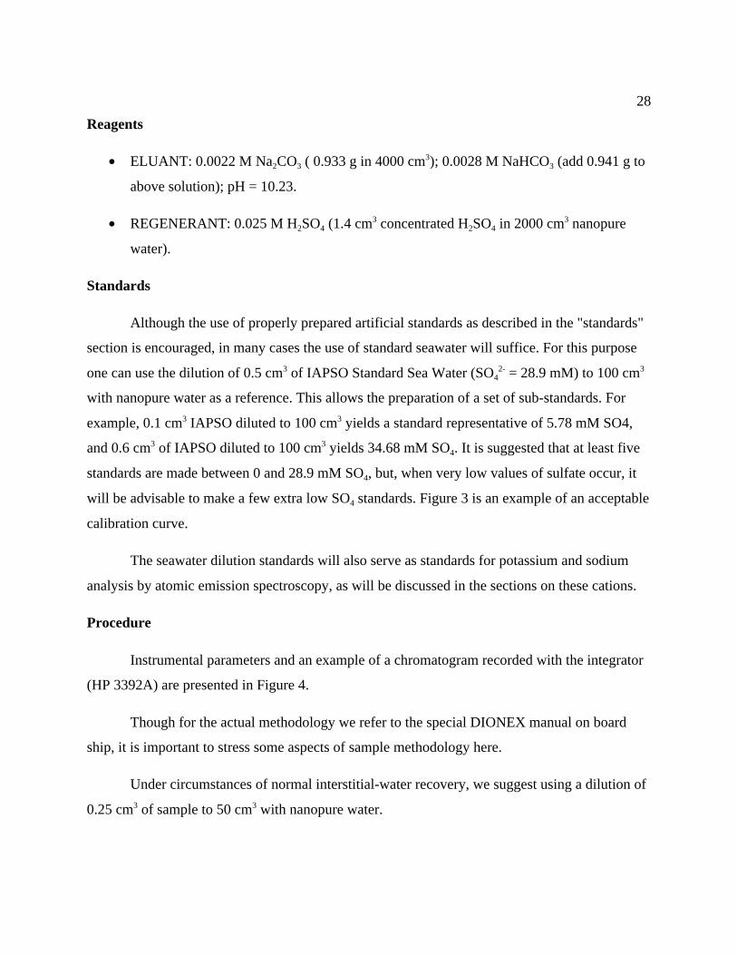
Although the use of properly prepared artificial standards as described in the "standards"

section is encouraged, in many cases the use of standard seawater will suffice. For this purpose

one can use the dilution of 0.5 cm3 of IAPSO Standard Sea Water (SO42- = 28.9 mM) to 100 cm3

with nanopure water as a reference. This allows the preparation of a set of sub-standards. For

example, 0.1 cm3 IAPSO diluted to 100 cm3 yields a standard representative of 5.78 mM SO4,

and 0.6 cm3 of IAPSO diluted to 100 cm3 yields 34.68 mM SO4. It is suggested that at least five

standards are made between 0 and 28.9 mM SO4, but, when very low values of sulfate occur, it

will be advisable to make a few extra low SO4 standards. Figure 3 is an example of an acceptable

calibration curve.

The seawater dilution standards will also serve as standards for potassium and sodium

analysis by atomic emission spectroscopy, as will be discussed in the sections on these cations.

Procedure

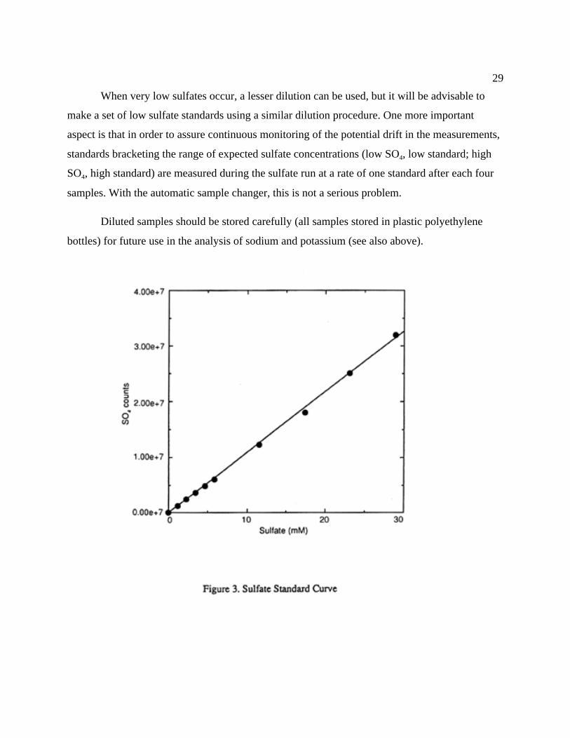
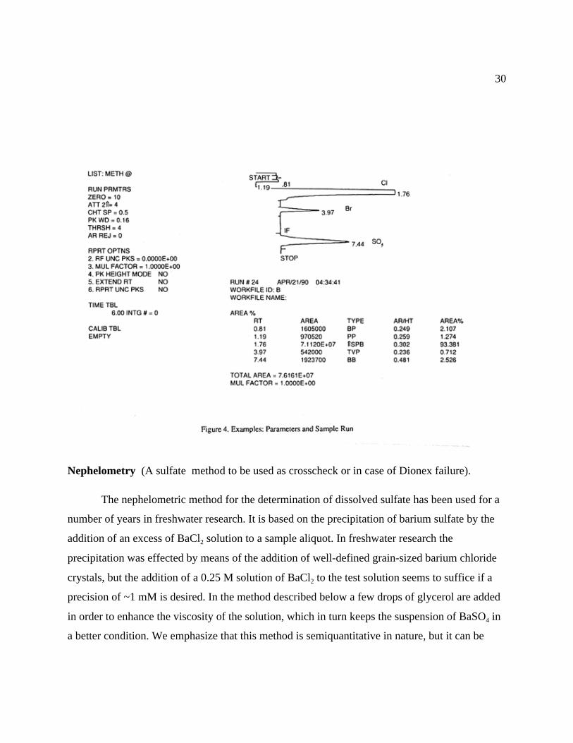
Instrumental parameters and an example of a chromatogram recorded with the integrator

(HP 3392A) are presented in Figure 4.

Though for the actual methodology we refer to the special DIONEX manual on board

ship, it is important to stress some aspects of sample methodology here.

Under circumstances of normal interstitial-water recovery, we suggest using a dilution of

0.25 cm3 of sample to 50 cm3 with nanopure water.

29

When very low sulfates occur, a lesser dilution can be used, but it will be advisable to

make a set of low sulfate standards using a similar dilution procedure. One more important

aspect is that in order to assure continuous monitoring of the potential drift in the measurements,

standards bracketing the range of expected sulfate concentrations (low SO4, low standard; high

SO4, high standard) are measured during the sulfate run at a rate of one standard after each four

samples. With the automatic sample changer, this is not a serious problem.

Diluted samples should be stored carefully (all samples stored in plastic polyethylene

bottles) for future use in the analysis of sodium and potassium (see also above).

30

Nephelometry (A sulfate method to be used as crosscheck or in case of Dionex failure).

The nephelometric method for the determination of dissolved sulfate has been used for a

number of years in freshwater research. It is based on the precipitation of barium sulfate by the

addition of an excess of BaCl2 solution to a sample aliquot. In freshwater research the

precipitation was effected by means of the addition of well-defined grain-sized barium chloride

crystals, but the addition of a 0.25 M solution of BaCl2 to the test solution seems to suffice if a

precision of ~1 mM is desired. In the method described below a few drops of glycerol are added

in order to enhance the viscosity of the solution, which in turn keeps the suspension of BaSO4 in

a better condition. We emphasize that this method is semiquantitative in nature, but it can be

31

used for the following purposes:

1. The determination of dissolved sulfate in pore-water samples in case of failure of the

DIONEX analyzer.

2. The determination of dissolved sulfate on an ad-hoc basis to determine sulfate

concentrations on selected samples from pore waters in order to establish the

concentration range of samples.

3. Any routine checks on water quality of drilling fluids, potable water, etc.

Reagents

• BaCl2 SOLUTION: Make a roughly 0.25 M solution of BaCl2 (~10 g in 200 cm3

nanopure water) and filter the solution through a Whatman no. 1 paper.

• GLYCEROL: Put glycerol in an eye-drop bottle.

Procedure

The method requires about 0.05 to 0.3 cm3 of sample, depending on the sulfate

concentration. It appears prudent to start with small quantities, which can be augmented when

greater accuracy is required.

One (1) cm3 of nanopure water is added to a 10 cm3 glass vial with a snap cap. Add 0.1

cm3 (or any other appropriate amount) of sample or standard to the vial, followed by three drops

of glycerol. Then add 3 cm3 of the BaCl2 solution. Set the spectrophotometer at 400 nm and read

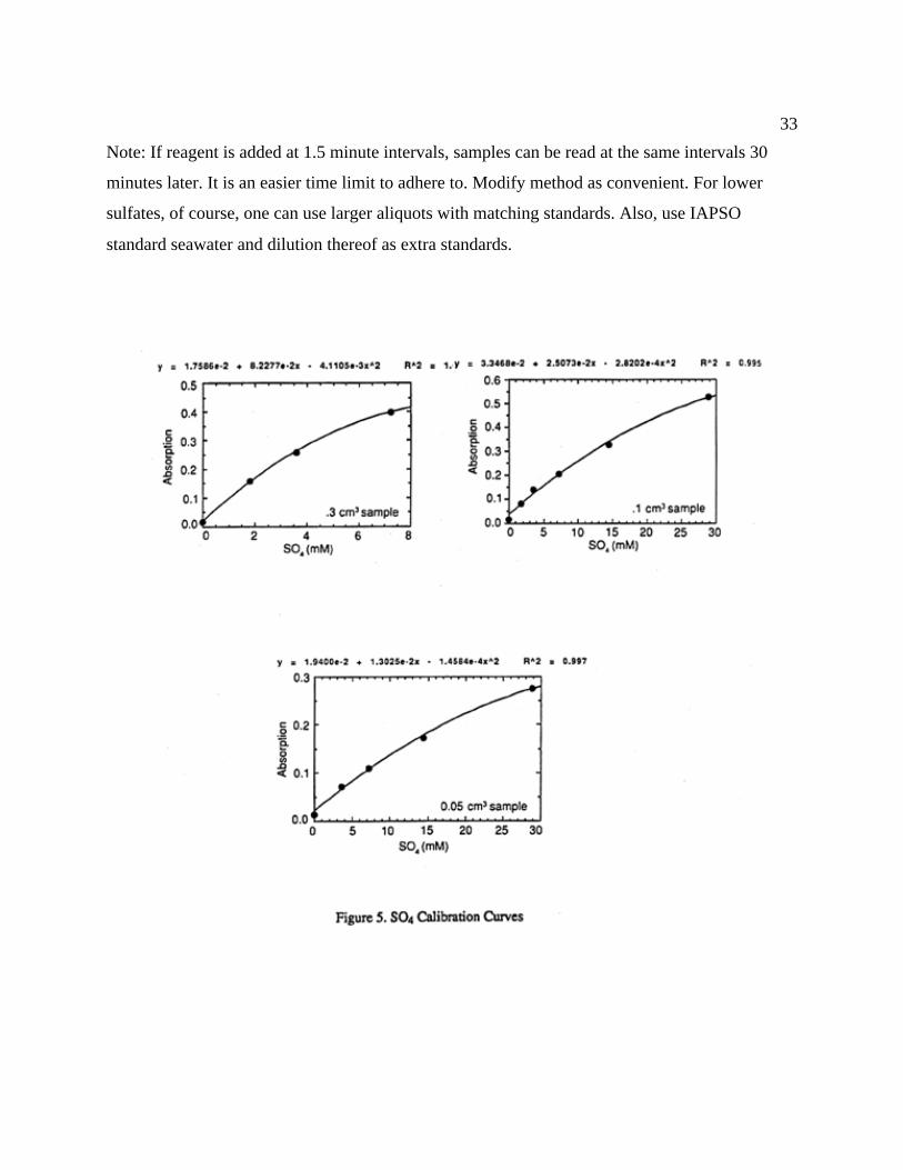
the absorbance. Plot the absorbance vs. standard curve.

Figure 5 indicates that there is no exact linear fit and that the accuracy suffers somewhat

at higher concentration levels. Nevertheless, reproducibility is quite good. The low-

concentration-range samples still show a reasonable precision.

32

Below we document an even better nephelometric method for sulfate determination.

The method uses a better stabilization of the barium sulfate suspension. The details were

provided through the courtesy of Dr. Rick Jahnke.

Reagents

• STOCK SULFATE SOLUTION: Dissolve 1.8141 g of K2SO4 in nanopure water and

dilute to 1 dm3. 1 M HCl: Add 85 cm3 concentrated HCl to 300 cm3 nanopure water and

dilute to 1 dm3.

• STOCK GELATIN SOLUTION: Dissolve 1.5 g of Difco-Bacto Gelatin (Detroit, MI) in

500 cm3 of hot (~70 C) nanopure water; cool, and store at 4 C for at least 16 hours before

use (bring water to 70 C on hot plate/stirrer, move flask to cold magnetic stirrer, add

gelatin, stir 15 minutes, let cool to room temperature and transfer to refrigerator). This

solution will be stable for about 28 days if kept in refrigerator.

• BARIUM/GELATIN REAGENT: Bring 150 cm3 of stock gelatin solution to room

temperature (by leaving it on the bench; do not heat on hot plate). Add 1.5 g of

BaCl2.2H2O and stir for 1 hour. Let stand 1 additional hour at room temperature and then

transfer to refrigerator. Stable for 7 days if kept cold.

Procedure

1. Add 10 cm3 of nanopure water to a large test tube as precisely as you can.

2. Add 500 L of 1M HCl.

3. Add 40 L of sample or standard.

4. At precise 1 or 1.5 minute intervals, add 500 L of Ba/Gelatin reagent; mix gently.

5. After 30 minutes plus/minus 10-15 seconds, read turbidity in spectrophotometer at 420

nm.

33

Note: If reagent is added at 1.5 minute intervals, samples can be read at the same intervals 30

minutes later. It is an easier time limit to adhere to. Modify method as convenient. For lower

sulfates, of course, one can use larger aliquots with matching standards. Also, use IAPSO

standard seawater and dilution thereof as extra standards.

34

BORON

The boron method is modified from a colorimetric technique described by Grinstead and

Snider (1967) and by Presley (1971). In this method the boron concentration is measured from

the formation of a boron-curcumin complex in acidic conditions, which shows an orange-red

color.

Reagents

• CURCUMIN: Dissolve 0.125 g of curcumin (C21O20H6) in 100 cm3 of glacial acetic acid.

• ACID REAGENT: Mix 50 mL of 96% sulfuric acid and 50 mL of glacial acetic acid.

• AMMONIUM ACETATE-ACETIC ACID: Dissolve 250 g of ammonium acetate plus

300 cm3 of glacial acetic acid in sufficient nanopure water to make 1 dm3.

Standards

Always choose standards that bracket the concentration range of the samples. This

curcumin method can be used to measure the concentration in pore-water samples which

typically contain 0-3 mM boron. It is therefore advisable to make standards of 0, 0.5, 1.0, 1.5,

......, 3.0 mM boric acid (in an artificial seawater matrix (0.6 M NaCl, 0.05 M MgCl2). In

addition, IAPSO standard seawater should be run (B = 0.45 mM). Standard solutions (and

samples) should be diluted in such a manner that the highest concentration does not exceed 0.5

mM.

A good stock solution will be 6.183 g of boric acid in 1 dm3 of nanopure water (=100 mM).

The procedure is outlined on the following page.

35

Boron Procedure

• Pipette a sample aliquot (25 µL or 50 µL) into a plastic bottle.

• Add 0.1 cm3 curcumin reagent.

• Add 0.4 cm3 acid reagent (with repipet), mix on vortex mixer, and wait for at least 30

minutes.

• Add 2.0 cm3 ammonium acetate-acetic acid buffer and mix.

• Measure absorbance at 555 nm in a 1 cm cell after 1.5 hours.

• Standard solutions should be run at the same time as the samples.

• Make a standard curve. If linear, read concentrations directly. If curved, use lower

concentration range of final solution.

CAUTION: If a crystalline precipitate forms after addition of the buffer (Step 4) it may be

necessary to use slightly less buffer, e.g., 1.9 cm3 (by trial and error).

36

IODIDE

In this method we really measure I- and IO3-, but in our DSDP/ODP samples we usually

work with samples from reducing environments in which the predominant species will be iodide

or an organic complex with iodide. The method was adapted from Pedersen (1979).

Reagents

• NaCl: 0.7 M (20.5 g NaCl/500 cm3 H2O).

• ACETATE BUFFER: 30 g NaAc in 1 dm3 flask, add 7 cm3 glacial acetic acid, make up

to 1 dm3 with distilled water.

• BROMINE WATER: saturated (fresh daily).

• FORMIC ACID

• KI: 10 g KI in 100 cm3 distilled water (make this fresh before use).

• SULFAMIC ACID: 1 g sulfamic acid (NH2SO3H) in 100 cm3 distilled water.

Standards

Always choose standards that bracket the range. Typically in Legs 67 and 111 samples

with high I (high NH4) we use: 0, 200, 400, 600, 800, 1000 M (use 0.7 M NaCl solution as

matrix) and then use 25 µL samples. If samples have much lower Iöe.g., typical anoxic box cores

would have 0~50 µM I– 0, 10, 20, 30, 40, 50 µM I standards and use 500 µL samples. Make sure

to bracket samples with the appropriate range of standards. A good stock solution is 0.415 g KI

in 250 cm3 distilled water (10 mM in I-). The procedure is outlined on the following page.

37

Iodide Procedure

1. Pipette a sample aliquot (25 µL or 500 µL--see above) into a glass vial.

2. Add 1 cm3 acetate buffer.

3. Add 0.04 cm3 bromine water (fresh), mix on vortex mixer, and gently heat on hot plate

for ~5 minutes (do not boil).

4. Allow to cool and add 0.1 cm3 of a 10% Na-azide solution (optional--if you fear NO2 is

present, this will kill the NO2).

5. After cooling to room temperature, add 0.04 cm3 formic acid and mix on vortex mixer.

6. Add 0.03 cm3 of 10% KI and 0.5 cm3 sulfamic acid solution and mix on vortex mixer.

7. Measure absorbance at 355 nm in 1 cm cell 3 minutes (±5 seconds) after KI is added.

8. Standards should be run at the same time as samples, using same aliquots.

9. Make a standard curve; if linear, you can read the I concentrations directly. If curved, use

lower concentration range of final solution.

38

BROMIDE

In the bromide method we make use of an adaptation of the iodometric method proposed

by Kremling (1983). In this method, use is made of sodium hypochlorite to oxidize both iodide

and bromide to iodate and bromate under alkaline conditions. Then this is reacted with fresh KI

solution in acidic medium to create iodine. This iodine is then measured with a

spectrophotometer (similar to the measurement of iodide). We found that both "reagent-grade"

and chlorox-grade hypochlorite has sufficient iodide/bromide in it to cause a rather large but

reproducible blank. We combat this blank by adding sufficient sodium thiosulfate to titrate the

excess iodine, thus making a good standard curve possible within a reasonable absorbance range

(0-1.5). The necessary blank must be determined by the individual investigator. The method has

also some time-dependent steps built in. A careful investigator, however, can obtain accuracy

better than 3% on 100 µL samples.

Reagents

• PHOSPHATE BUFFER: Dissolve 5 g sodium dihydrogen phosphate (NaH2PO4.H2O) in 100

cm3 volumetric flask and make to volume with double deionized water.

• SODIUM HYPOCHLORITE SOLUTION: Use reagent-grade sodium hypochlorite solution.

• SODIUM FORMATE SOLUTION: (HCOONa) 50% (w/v). Dissolve 15 g sodium hydroxide(NaOH) in ~50 cm3 water. Cool down to room temperature and add 16 cm3 of 90% formicacid (HCOOH) while stirring. Then dilute to 100 cm3.

• AMMONIUM MOLYBDATE SOLUTION: ((NH4)6Mo7O24.4H2O) 3% (w/v).

• SULFURIC ACID: (H2SO4) 3 M. Slowly add 16 cm3 concentrated sulfuric acid into 80 cm3

deionized water while stirring. Cool down to room temperature.

• POTASSIUM IODIDE: Dissolve 10 g KI in 100 cm3 double deionized water; make it fresh.

• SODIUM THIOSULPHATE SOLUTION: (Na2S2O3.5H2O) 0.6 mM. Pipette 3.5 cm3 of 0.05

M sodium thiosulphate solution (dissolve 3 g of Na2S2O3.5H2O in 250 cm3 double deionized

water) into a 250 cm3 volumetric flask; make to volume with deionized water.

39

Standards

STANDARD SOLUTION: Use NaBr solutions as standard series. Use IAPSO for comparison. If

all data fall on one standard curve, then of course there is no serious salt effect. For highly saline

solutions this should be double checked.

STANDARDS: Use 0, 500, 1000, 1500, 2000 µM NaBr solutions and IAPSO (860 µM) as

standards.

Procedure

1. Add 1.5 cm3 of phosphate buffer into a 5 cm3 glass vial.

2. Add 1.0 cm3 of distilled water.

3. Pipette a sample aliquot 25 to 100 µL (wash the tip of pipette with (1.+2.) solution severaltimes).

4. Add 0.25 cm3 sodium hypochlorite solution.

5. Heat the solution on a hot plate and boil for about 5 seconds.

6. Remove from the hot plate and add 0.5 cm3 sodium formate solution and cool down to roomtemperature.

7. Add 0.03 cm3 of molybdate solution.

8. Add 0.05 cm3 of 10% KI solution (fresh daily).

9. Add 0.3 cm3 of sodium thiosulphate solution and 0.75 cm3 of sulfuric acid.

10. Measure absorbance at 355 nm in 1 cm cell 10 minutes after sulfuric acid is added (waitabout 1 minute after sucking the solution into the cell, then write down the reading ofabsorbance).

11. Standard solutions should be run at same time as samples using same aliquots.Make astandard curve; if linear, you can read the Br concentrations directly. If curved, use lowerconcentration range of final solution or adjust the added amount of sodium thiosulphate solution.

Note: Please do not forget to correct for the iodide content; this method determines total I + Br.

40

AMMONIUM

The determination of ammonium concentrations is of importance because this constituent

is an indicator of the diagenesis of organic matter in the sediments. The onset of sulfate reduction

coincides with the start of ammonium ion production. The production of ammonium, however,

appears to increase strongly in the zone of methanogenesis, presumably as a result of associated

deammonification reactions. The large potential variation in ammonium concentrations,

therefore, suggests that a few preliminary ammonium concentrations should be run in order to set

limits to the sample dilution and range of standards to be used. Suggestions for this follow

below.

The methodology is based on the method of Solorzano (1969), originally developed to

detect very small NH4+ concentrations in seawater. Although blank problems in seawater are

enormous, the relatively high concentrations in pore fluids (up to 85 mM in Leg 112 samples;

Kastner et al., 1990) reduce this blank problem. In areas of slow sedimentation, however, very

low ammonium concentrations require great caution to avoid this problem. The method is based

on the diazotization of phenol and the subsequent oxidation of the diazo compound by chlorox to

yield a blue color.

Method

Reagents

• PHENOL-ALCOHOL SOLUTION: Dissolve 0.8 g reagent-grade crystalline phenol in

100 cm3 95% ethyl alcohol. Make fresh each day of use. Instead of the crystalline phenol,

1 cm3 of liquified phenol can be used.

• SODIUM NITROPRUSSIDE SOLUTION: Dissolve 0.15 g sodium nitroprusside

(sodium nitroferricyanide) in 200 cm3 of nanopure water (make fresh each day).

• ALKALINE SOLUTION: Dissolve 7.5 g of trisodium citrate and 0.4 g sodium hydroxide

in 500 cm3 nanopure water. This is a fairly stable solution.

41

• OXIDIZING SOLUTION: Add 1 cm3 fresh sodium hypochlorite (4% available

chlorine)– chlorox will do equally well–to 50 cm3 alkaline solution and use the same day.

• AMMONIUM STANDARD: Dry ammonium chloride in oven overnight. Dissolve 5.345

g ammonium chloride in 1 dm3 of nanopure water. One can also use non-dried NH4Cl and

determine the chloride content of the standard solution by means of a chloride titration.

For reasonable accuracy, use a 0.5 cm3 aliquot (Cl = 0.1M) to obtain almost the same

concentration of Cl as in IAPSO reference standard seawater.

Procedure

For each specific area, different concentrations of ammonium may occur. Typically in

areas with a strong evidence of organic-carbon diagenesis (e.g., organic-carbon-rich sediments),

very high concentrations of NH4 can be expected. In that case, sample aliquots must be made

appropriately small, and indeed sample dilution may be required. The range can be established

easily by using a sample near the alkalinity maximum. Once the range has been determined,

standards must be prepared that cover this range. In this manner samples and standards are

treated in a similar way. Below we describe the procedure for relatively low ammonium

concentrations. Care should be taken to use clean glass vials, preferably not used for Si and PO4

determinations, in which ammonium molybdate is used as a reagent.

Use a 100 lambda (100 microliters) Eppendorf pipette to transfer 0.1 cm3 of sample to a 5

cm3 glass vial. Add 1 cm3 nanopure water to each, then 0.5 cm3 phenol-alcohol solution, 0.5 cm3

sodium nitroprusside, and finally 1 cm3 of oxidizing solution. Adding these solutions with

Eppendorf pipettes is fast and convenient and ensures proper mixing during addition. Shake

samples after each addition. Standards should range from 0 to 1000 µM, or any other appropriate

range as discussed above. Let the color develop for at least 1 hour (longer would be better, up to

3 hours) and then determine the absorbance at 640 nm wavelength.

42

SILICA

Dissolved silica determinations are of great importance in interstitial waters. Often they

represent the lithology of the sediments, and the concentrations can vary widely, especially if

highly dissolvable phases such as biogenic opal-A, volcanic ash, or smectite are present. Thus a

wide range of concentrations can be expected, typically from 50 to 1200 µM or higher

(especially in hydrothermally affected sediments). Thus the method below usually covers the

range, although greater dilutions may become appropriate if sediments or sample sizes

necessitate this.

The method is based on the production of a yellow silicomolybdate complex and the subsequent

reduction of this complex to yield a blue color. The blue complex is very stable, which will

enable delayed reading of the samples.

Method

Reagents

• MOLYBDATE REAGENT: Dissolve 4 g of ammonium paramolybdate,

(NH4)6Mo7O24.4H2O (preferably fine crystalline), in ~300 cm3 nanopure water using a 500

cm3 volumetric flask. Add 12 cm3 concentrated hydrochloric acid (12N), mix, and make

up the volume to 500 cm3 with nanopure water. This reagent is stable for many months if

stored in a dark bottle. The reagent should be discarded immediately when any white

precipitate forms. If unable to store properly, or if time permits, make fresh for each run.

• METOL SULFITE SOLUTION: Dissolve 6.0 g anhydrous sodium sulfite, Na2SO3, in a

500 cm3 volumetric flask. Add 10 g Metol (p-methylaminophenol sulfate) and then

nanopure water to make the volume to 500 cm3. When the metol has dissolved, filter the

solution through a Whatman no.1 filter paper and store in a clean glass bottle, preferably

dark glass, which is tightly stoppered in the refrigerator. This solution may deteriorate

quite rapidly and erratically so it should be prepared fresh every month.

43

• OXALIC ACID SOLUTION: Prepare a saturated oxalic acid solution by shaking 50 g

of analytical-grade oxalic acid dihydrate, (COOH)2.2H2O, with 500 cm3 of nanopure

water. Let stand overnight. Decant solution from crystals before use. This solution is

stable and can be stored in a glass bottle.

• SULFURIC ACID SOLUTION: 50% v/v. Using a 500 cm3 volumetric flask, pour 250

cm3 concentrated analytical-grade sulfuric acid into ~200 cm3 nanopure water. Cool to

room temperature and bring volume to 500 cm3 with a little extra water. Store in a

polyethylene bottle.

• REDUCING SOLUTION: Mix 50 cm3 Metol sulfite solution with 30 cm3 oxalic acid

solution. Add slowly, with mixing, 30 cm3 50% sulfuric acid solution and bring volume

to 150 cm3 with nanopure water. This solution should be made daily, just before using it.

• SYNTHETIC SEAWATER: Dissolve 25 g sodium chloride (NaCl) and 8 g of

magnesium sulfate heptahydrate (MgSO4.7H2O) in 1 dm3 of nanopure water and store in a

polyethylene bottle. The silica content of the solution should not exceed 1-2 M.

Standards

SILICATE STANDARD: Use is made of sodiumsiliocofluoride (Na2SiF6) for this purpose.

When dissolved in water, this substance hydrolyzes to form reactive dissolved silica. The

Na2SiF6 is placed in an open plastic vial and placed in a vacuum desiccator overnight to remove

excess water. Do not heat or fuse.

PRIMARY STANDARD: Dissolve 0.5642 g of Na2SiF6 in a 1 dm3 polyethylene volumetric

flask. Dissolution is slow, so allow at least 3 minutes. This cannot be rushed. Use nanopure water

for this purpose. The concentration of the standard is 3000 µM. Store in a 500 cm3 polyethylene

bottle. The standard is stable indefinitely.

44

DILUTIONS FROM PRIMARY STANDARD: When making dilutions, use distilled water

and store in polyethylene containers. Using a 50 cm3 volumetric flask, add the following

amounts of primary standard and then bring to a total of 50 cm3:

30 µM Si 0.5 cm3 primary standard60 1.0120 2.0240 4.0360 6.0480 8.0600 10.0900 151200 20 et cetera

Method

1. First, make sure that all reagents are prepared ahead of time. The method has a time factor

built in, and therefore it is of great importance to have all necessary reagents ready to go.

2. Label and set up 3-dram plastic vials and caps (well washed with nanopure water).

3. Measure into the vials 4.0 cm3 of silica free nanopure water (3.8 cm3 for standards and blank).

4. For standards and blank only, pipette in 0.2 cm3 of synthetic seawater.

5. Pipette 0.2 cm3 of sample or standard or blank (nanopure water) into the vial with an

Eppendorf pipette.

6. Record time.

7. Add 2.0 cm3 of molybdate solution to the vials. A yellow color will develop, and this is

allowed to mature for exactly 15 minutes (±15 seconds). Then add 3.0 cm3 of the reducing

solution. Cap the vials and let stand for at least 3 hours.

8. Read absorbances on the spectrophotometer at 812 nm. Please consult procedural notes of the

following page.

45

Notes:

Do not handle more than about 30 samples at a time in order to ensure that the 15- minute

time limit can be adhered to. Make sure that there are no wild fluctuations in room temperature,

which is not normal in an air-conditioned room.

Do not use synthetic seawater in dilutions of the primary standard. This could cause the

decrease in reactive silica in a few hours as a result of polymerization reactions.

The reason for adding 0.2 cm3 of synthetic seawater to the standards is to maintain a

reasonably uniform salt content in relation to the samples, thus suppressing a potential salt effect

on the method.

Although it is suggested that strict adherence to the 15-minute time limit is advisable,

tests have shown that there is some leeway, i.e., the yellow molybdate complex is stable from 10

to 20 minutes. However, consistency in the time limit will eliminate any potential error.

It is important to wait at least 3 hours for the blue color to develop; the higher the

concentration, the longer the time. The color remains stable for many more hours, and reading

after 4 or 5 hours may, in fact, be a good idea. Again, consistency in time limits is advisable.

46

PHOSPHATE

The determination of dissolved phosphate, particularly in rapidly deposited organic-

carbon-rich sediments, is important in the shipboard analytical program. Phosphate

concentrations may vary considerably, and it is therefore advisable to obtain a preliminary idea

of the concentration ranges to be expected. This can most easily be accomplished by taking

samples in the region of maximum alkalinities, especially if these maximum values occur within

50 to 100 mbsf. Typically if alkalinities attain more than 30 mM, dissolved phosphate

concentrations can attain more than 100 µM. Thus, only very small sample aliquots will be

needed to establish the concentration range. The method is, in essence, the colorimetric method

described by Strickland and Parsons (1968) as modified by Presley (1971) for DSDP pore fluids.

It is important to note that the concentration in the final test solution cannot exceed more

than about 10 µM. Thus, for open-ocean (low sedimentation rate, low organic carbon) samples,

one might need to do the determination on 2 cm3 of sample (expected range 0-10 µM), but in

typical continental-margin settings, where concentrations can exceed 100 or 200 µM, a 0.1 or 0.2

cm3 sample aliquot must be used. As mentioned above, the concentration range must be

established prior to running the samples, and it is highly advisable to make standards that cover

the range of concentrations to be expected. In this manner, standards and samples will all get the

same treatment.

Reagents

• AMMONIUM MOLYBDATE SOLUTION: Dissolve 2 g (NH4)6Mo7O24.4H2O in

1000 cm3 of nanopure water. The solution is stable indefinitely if stored in a

plastic bottle.

• SULFURIC ACID SOLUTION: Dilute 10 cm3 of concentrated H2SO4 (specific

gravity 1.82 g/cm3) to 1000 cm3 with nanopure water.

• ASCORBIC ACID SOLUTION: Dissolve 3.5 g ascorbic acid in 1000 cm3 of

47

nanopure water. This solution must be kept refrigerated and should not be

stored for more than a week.

• POTASSIUM ANTIMONYL-TARTRATE SOLUTION: Dissolve 0.09 g of

KSbC4H4O7.1/2H2O in 1000 cm3 of nanopure water. This solution is stable for

many months.

• MIXED REAGENT: Mix together 50 cm3 ammonium molybdate, 125 cm3

sulfuric acid, 50 cm3 ascorbic acid, and 25 cm3 potassium antimonyl-tartrate. Do

not store this solution for more than a few hours. It is best to prepare the mixed

reagent immediately before making the determinations.

• PHOSPHATE STANDARD: Dissolve 1.3614 g KH2PO4 in 1000 cm3 of nanopure

water. This yields a 0.01 M phosphate standard solution which lasts quite a long

time, unless there is evidence for growth of algae or other extraneous biotic

material. It should be remembered that the range of expected concentrations

should be established first, then the appropriate standards can be prepared and the

proper dilution factor chosen.

Procedure

Put the appropriate aliquot of sample or standard in a small glass vial (~5 or 10 cm3 size),

e.g., 1 cm3 for "open ocean" sites, 0.1 or even 0.01 cm3 for high organic carbon, high alkalinity

sites. In the latter case one ought to add about 1 cm3 of nanopure water, the main thing being that

in no case the final concentration of phosphate is more than 10 µM. Add 2 cm3 of mixed reagent.

After a few minutes a blue color develops, which remains stable for a few hours. For these

reasons it is best to make the readings of the absorbance at 885 nm about half an hour after the

addition of the mixed reagent. Use 1 cm cells.

48

NITRITE

Under normal circumstances the need for determination of the nitrite concentration of

ODP samples is limited unless, perhaps, drilling is in areas of very slow sedimentation, where

dissolved oxygen may penetrate to considerable depth into the sediment column. In such a case,

redox reactions involving nitrate reduction, which often is accompanied by an intermediate

production of nitrite, may be detectible at greater depths. Prime candidates for such sites are

areas of red clays or extremely slow carbonate deposition. In any case, the method needs to be

described because it is used in the method of nitrate determination, in which nitrite is produced

by a reductive technique. The method is based on an adaptation of the method proposed by

Strickland and Parsons (1968). In the method, nitrite is allowed to react with sulfanilamide in an

acid solution. The resulting diazo-compound reacts with N-(1-naphtyl)-ethylene diamine to form

a pink azo dye, whose absorbance is measured at 543 nm.

Reagents

• SULFANILAMIDE SOLUTION: Dissolve 5 g of sulfanilamide in a mixture of 50 cm3

concentrated HCl (1.18 g/cm3) and ~300 cm3 of nanopure water. Dilute to 500 cm3. The

solution is stable for many months.

• N-(1-NAPHTYL)-ETHYLENE DIAMINE DIHYDROCHLORIDE SOLUTION: Dissolve

0.50 g dihydrochloride in 500 cm3 of nanopure water. Store in dark bottle. The solution

should be made prior to the determinations. It will be stable for only a short time (a few

weeks at best).

Procedure

Add 0.1 cm3 of the sulfanilamide solution to a 2 cm3 sample and allow reaction for 2-8

minutes (make sure this is done in a reasonably consistent manner). Then add 0.1 cm3 of naphtyl

ethylene diamine dihydrochloride solution and mix immediately. A nice pink color develops

immediately if nitrite is present. After 10 minutes, but before 2 hours has elapsed, measure at

543 nm in the 1 cm path length, flow-through cell. Use nanopure water as a blank.

49

NITRATE

Nitrate concentrations, especially in open-ocean sediments with low sedimentation rates,

can be useful indicators of diagenetic processes involving organic carbon. For these reasons it

will be useful to have this method available on board ship, even though the methodology is

relatively laborious and will probably be used only when sampling programs are not too busy.

Generally, concentration ranges will be between 0 and 60 µM.

Often a good judgment can be made for the potential use of the nitrate method on the

basis of the ammonia measurements. If the latter rise very quickly above 50 µM, it is almost

certain that little or no nitrate will be present but rather that the zone of sulfate reduction has

been entered.

The method is adopted from Strickland and Parsons (1968) and makes use of the catalytic

reduction of nitrate to nitrite, using a cadmium reduction column. A peristaltic pump (of

autoanalyzer type) is used to force the samples and standards through the reduction columns. The

use of only one channel of the pump is advocated to keep better track of the samples and

standards. It should be remembered that each and every one of the columns has its own

individual characteristics.

Column Preparation

There are two types of suggested columns:

1. Teflon tubing of 3 mm internal diameter. Put a small amount of glass wool in the

bottom of the teflon tube (fine copper wool is supposed to be preferable). Fill about 5

cm length of the tubing with small (0.5 to 2 mm) Cd chips. Put a small amount of

glass or copper wool on top of the loosely packed column.

2. A more preferred method is to use < 1 mm (i.d.) tygon tubing and fill this with

cadmium wire. A thin piece of copper wire can be used on both sides of the cadmium

wire.

50

Of importance is to note that the columns, after their activation as described below,

remain out of contact with air because they will get poisoned. Also avoid contact with hydrogen

sulfide-containing solutions. They will produce CdS and finish the columns. The columns get

attached to 1/16-inch-by-1/8-inch tygon tubing which can be used in the peristaltic pump or at

the other end. When not in use, keep both ends in water to prevent aeration of the columns.

Intake------peristaltic pump------column------outflow.

Activation of the column(s) can be achieved as follows. (If starting with a new, clean Cd

column, step 1 may be eliminated.)

1. Pass 5% HCl through the columns for a few minutes, then wash with nanopure water

until the effluent has a neutral pH.

2. Pass a 2% copper sulfate solution through the column for a few minutes (10-20 cm3),

followed by a wash with dilute ammonium chloride (see below). The column is now

ready.

Reagents

• CONCENTRATED NH4Cl: 175 g of NH4Cl in 500 cm3 of nanopure water. This solution is

used for buffering of samples and standards.

• DILUTE NH4Cl: 50 cm3 of concentrated NH4Cl diluted to 2000 cm3. This solution is used for

washing the columns.

• SULFANILAMIDE SOLUTION (as in the nitrite method): Dissolve 5 g of sulfanilamide in

a mixture of 50 cm3 concentrated HCl (1.18 g/cm3) and ~300 cm3 of nanopure water. Dilute

to 500 cm3. The solution is stable for many months.

• N-(1-NAPHTYL)-ETHYLENE DIAMINE DIHYDROCHLORIDE SOLUTION (as in the

nitrite method): Dissolve 0.50 g N-(1 naphthyl)-ethylene diamine dihydrochloride in 500 cm3

of nanopure water. Store in dark bottle. The solution should be made prior to the

determinations. It will be stable for only a short time (a few weeks at best).

51

Procedure

If a column has not been used recently, it is advisable to run a few standards through it to

check the column's activity. If it appears that there may be a problem, it is advisable to make new

columns. In any case, columns do not last too long and are usually soon in a state of deterioration

when not used regularly.

Before running samples through the column, do a pre-rinse using dilute NH4Cl.

Use 1 cm3 of sample or standard and add 4 cm3 of nanopure water. Add 0.1 cm3 of

concentrated NH4Cl solution as a buffer. Run the buffered sample through the column at a speed

of ~3-5 cm3/minute. Collect the last 4 cm3. For the actual analysis of the nitrite, only 2 cm3 is

used, as described above in the nitrite method.

After all the samples have been run through the column, a wash with dilute NH4Cl is

advisable for the duration of at least several minutes. Also make sure that the intake tube and the

outlet tube remain submersed in water in order to prevent any inadvertent contamination of the

reduction column.

Standards are made from a stock solution of 10 mM KNO3. The range of the standards

should be 0-60 µM. It is best to prepare the standards in synthetic seawater: 30 g NaCl, 10 g

MgSO4.7H2O, 0.05 g NaHCO3 in 1000 cm3 of nanopure water.

52

ATOMIC ABSORPTION METHODS

With the purchase of the Varian SpectrAA-20 Atomic Absorption Spectrometer, it is now

possible to determine various elements in the interstitial waters that previously could not be

determined. Below we describe methods for the following elements:

Alkali metals: Li, Na, K, and Rb.

Alkaline earths: Sr.

Other elements can be added to this list, in particular Mn.

The notes below are based in part on a method described by Hans Brumsack, who used

the method extensively during ODP Leg 127 in the Japan Sea. Sections of the unpublished

Brumsack report are paraphrased here with the author's permission.

ALKALI METALS

Brumsack cites several excellent reasons why the determination of alkali metals ought to

be done in the flame-emission mode (AES) of the instrument:

• For the determinations, an element-specific lamp is not required.

• Detection limits are generally lower and allow determination even of the rarer alkali metals

from diluted samples.

• The working range is variable owing to the adjustable photomultiplier voltage.

Instrument Setting

As a general rule, AES determinations should be performed with a small slit width,

preferably at 0.2 nm (the smallest width available on the Varian AA-20). For K, Li, and Rb use

can be made of the normal acetylene/air burner head in its lengthwise position. The burner head

slit can be aligned along the light path using a small piece of paper to reflect the light beam as it

53

travels along the slit towards the detector. The optimization routine within the software

package can then be used to attain greater precision of light through the flame in the absorbance

mode using the appropriate hollow cathode lamp. In order to reduce sensitivity for Na, however,

the burner should be rotated perpendicular to the light source to minimize the detected reaction

inside the flame.

Final optimization must be done in the emission mode using the highest standard as a reference.

Prior to use, it is advisable to clean the burner head by aspirating nanopure water. In

addition the flame should be lighted at least 20 minutes before use to allow the instrument to

stabilize.

Sample Preparation

All diluted samples are best stored in nanopure-rinsed polyethylene vials, especially

because glass vials may cause problems with exchange of alkali metals.

For the determination of K and Na, use is made of the samples that have been diluted

previously for the determination of sulfate, i.e., 0.25 cm3 of pore water in 50 cm3 nanopure water.

For both alkalis the following dilution is used to obtain a calibration curve:

1 cm3 of SO4 dilution + 8 cm3 nanopure water + 1 cm3 3.5 weight% CsCl. The CsCl is used as an

ionization buffer.

For Li, separate dilutions are made, with special attention given to the range of

concentration anticipated:

Near the surface, with Li concentrations near 25 µM, a 5-times dilution is prepared, e.g.,

0.5 cm3 sample/standard + 2.0 cm3 nanopure water. At higher Li concentrations, use up to a 20-

times dilution.

N.B. No Cs is needed because the Na in seawater or pore water acts as an ionization buffer.

Rb concentrations are usually quite low in the sediments and require either little dilution

54

or should be done directly on seawater or should be saved for more sophisticated work in the

shore laboratory. If ample sample is available, however, the methodology described below will

be advisable.

Standard Solutions

Potassium (766.5 nm, slit 0.2 or 0.5 nm)

In many pore-water profiles, slightly higher than seawater concentrations of K are often

observed, but at greater depths one usually observes a decrease in the K concentration. Thus

standards of the same dilution as the sulfate dilutions are prepared. Use can be made of standard

seawater for this purpose.

The following dilutions are recommended:

cm3 IAPSO (diluted to 100 cm3) 0.05 0.10 0.25 0.50 0.75 1.00.

mM K (representative) 1.04 2.09 5.20 10.4 15.70 20.9.

Of course, individual standards can also be prepared in nanopure from the 1000 ppm K

Atomic Absorption Reference Standard Solution.

Sodium (589.0 nm, slit 0.2 or 0.5 nm)

The sodium determination requires the utmost accuracy in order to beat the estimate by

charge balance calculation. In a later comment we will show a comparison of Na-experimental

and Na-calculated, which will confirm good agreement. However, the data obtained by

calculation (heavily dependent on the accuracy of chloride determinations) show less scatter. On

the other hand, the determination of Na does not require extra samples and can serve as a good

check on the overall accuracy of charge balance calculated values.

55

Standards can be produced most easily by appropriate dilution of IAPSO standard seawater

(same dilution as sulfate):

cm3 IAPSO (diluted to 100 cm3) 0.1 0.2 0.4 0.45 0.5 0.55 0.6

mM Na (representative) 96 192 384 432 480 528 576

Again, as with K, extra standards can be prepared with the 1000 ppm Atomic Absorption

Reference Standard Solution.

Lithium (670.8 nm, slit 0.2 nm or smaller)

Lithium often shows considerable change in the pore fluids, ranging from 27 µM in

seawater to both lower and considerably higher values. For these reasons it is important to assess

the concentration range, using a few samples from each hole at strategic intervals. However, it is

most advisable to prepare standards over a range from 27 to 1000 µM. Dilutions of a 50 µM LiCl

stock solution are best made with surface seawater, whose known chloride concentration allows

the calculation of the Li concentration with respect to that of IAPSO standard seawater. This can

be done because Li is a conservative component of seawater, i.e., its Li/Cl ratio is constant for all

intents and purposes. The reason why surface seawater is used for this purpose is that seawater

has a large sodium concentration, thus allowing for the ionization buffer (as described above).

Standards can be produced from surface seawater (SS) and 50 mM LiCl:

cm3 50 mM Li 0 0.1 0.2 0.3 0.4 0.5 1.0 1.5 2.0

(diluted to 100 cm3)

µM Li 27 77 127 177 227 277 527 777 1027

(representative)

Typically, one can start with a 5-times dilution (0.5 cm3 to 2.5 cm3 with nanopure water)

of both standards and samples, which may be increased to greater dilutions as Li concentrations

56

increase with depth. During Leg 131 we used at most a 20-times dilution (0.1 cm3 in 2 cm3 of

nanopure water).

Rubidium (780 nm, slit 0.2 nm)

Rubidium shows distribution patterns similar to K, i.e., concentrations in surface cores

close to seawater (1.4 µM), whereas below this a concentration similar to that of potassium is

followed, with the exception of hydrothermal situations, in which quite high concentrations can

occur (c.f. Gieskes et al., 1982).

Standards are best prepared over a range of 0 to 10 µM in a solution containing about 475

mM NaCl. This mimicks the Na concentration of IAPSO standard seawater, sodium being the

ionization buffer. Again it is best to start optimization with a 3 M Rb standard solution in most

situations, the higher standards being available if needed in special situations. Do not forget to

run a blank test on the 475 mM NaCl solution from which the standards are made.

Analysis

Especially in the case of the determinations of Li and Rb it is most important to work

with the slit width at 0.2 nm. The Varian AA sets the photomultiplier voltage automatically. For

the optimization it is therefore important to optimize with a standard of at least 20% higher

concentration than any of the expected values. This is to ensure that the intensity of emission will

fall in the linear range of the instrument. In addition it is advisable to rinse the instrument burner

head by aspiration with nanopure water after each measurement. Frequent replacement of the

nanopure water is necessary so that no salt buildup occurs in the nanopure water. In addition it is

important to intersperse standards every five determinations, choosing a standard close to the

concentrations being measured. Any drift can be followed easily in that fashion.

The delay time should be set at 3-5 seconds. The integration time should be 4 seconds.

Replicates should be 3 to 5 times. Make sure the gas flow remains constant, and check the tubing

of the aspirator regularly for evidence of blockage. Slower aspiration can be as damaging as

irregular gas flow.

57

During Leg 131 we found that the instrument performed beautifully.

N.B. When doing the sodium in the pore fluids of Leg 131 we found a satisfactory

relation between calculated and determined Na. The database for Na calculations gave a

smoother concentration depth profile than the measured data. On the other hand, doing the Na

determinations yields an opportunity to double check on the calculations and therefore on the

entire database. As the sodium determination is carried out on the potassium dilutions, no extra

sample preparation is involved.

OTHER CONSTITUENTS

The AA is also most useful for the determination of other constituents of pore fluids, e.g.,

strontium, manganese, calcium, and magnesium. The latter two can be determined more

accurately by titration, but the AA can serve as a backup as well as a check on the titration data

when any doubts arise. As always, the first thing is to make dilutions of samples and standards in

such a manner that the concentrations of the test solutions do not exceed the specifications of the

instrument. In addition one should make sure that the manufacturer's suggestions for background

buffers (e.g., lanthanum chloride in sufficient amounts for Ca and Mg) are adhered to.

During Leg 131, as an example, we studied the distribution of strontium in the pore

fluids. For this purpose we made standards in surface seawater using spikes of Sr to reach a

range of 87 to 1000 µM. In addition, Sr standards can be prepared from the available 1000 ppm

Atomic Absorption Reference Standard Solution.

A 50,000 ppm La (as LaCl3) is used to spike the solution:

0.2 cm3 of sample/standard Of course, one can make appropriate variations on

+ 1.6 cm3 nanopure water. this as the need arises

+ 0.2 cm3 50,000 ppm La.

58

The results were most satisfactory. Of course, if two types of standards are used, one

with and one without Na, the agreement in standard curves will serve as proof that La did the

trick.

N.B. It will really pay off to read the manuals first before starting AA work. It can be an

enormous time saver. All the manuals are available in the chemistry laboratory.

59

REFERENCES

Bates, R. G., and Calais, J. G., 1981. Thermodynamics of the dissociation of Bis.H+ in sea water

from 5 to 40°C. J. Solution Chem., 10:269-279.

Bates, R. G., and Culberson, C. H., 1977. Hydrogen ions and the thermodynamic state of marine

systems. In Anderson, N. R., and Malahoff, A. (Eds.), The Fate of Fossil Fuel CO2 in the

Oceans: New York (Plenum Press), 45-61.

Brumsack, H., Notes on Atomic Absorption, Leg 127 (in press).

Gieskes, J. M., and Lawrence, J. R., 1976. Interstitial water studies, Leg 35. In Hollister, C. D.,

Craddock, C., et al., Init. Repts. DSDP, 35: Washington, DC (U.S. Govt. Printing Office), 407-

424.

Gieskes, J. M., and Rogers, C., 1973. Alkalinity determination in interstitial waters of marine

sediments. J. Sed. Petrol., 43:272-277.

Gieskes, J. M., and Peretsman, G., 1986. Water chemistry procedures aboard JOIDES

Resolution--some comments. ODP Technical Note 5: College Station, TX (Ocean Drilling

Program).

Gieskes, J. M., Elderfield, H., Lawrence, J. R., Johnson, J., Meyers, B., and Campbell, A. C.,

1982. Geochemistry of interstitial waters and sediments, Leg 64, Gulf of California. In Curray, J.

R., Moore, D. G., et al., Init. Repts. DSDP, 64(2): Washington, DC (U.S. Govt. Printing Office),

675-694.

Grinstead, R. R., and Snider, S., 1967. Modification of the Curcumin method for low level boron

determinations. Analyst, 92:532-533.

Kastner, M., Elderfield, H., et al., 1990. Diagenesis and interstitial water chemistry at the

Peruvian Margin--major constituents and strontium isotopes. In Suess, E., von Huene, R., et al.,

Proc. ODP, Sci. Results, 112: College Station, TX (Ocean Drilling Program), 413-440.

60

Khoo, K. H., Ramette, R. W., Culberson, C. H., and Bates, R. G., 1977. Determination of

hydrogen ion concentrations in sea water from 5 to 40°C: standard potentials at salinities from 20

to 45%. Analytical Chem., 49:29-33.

Kremling, K., 1983. Determination of major constituents: bromide. In Grasshoff, K., Ehrhard,

M., and Kremling, K. (Eds.), Methods of Sea Water Analysis. New York (Springer Verlag).

Pedersen, T. F., 1979. The geochemistry of sediments of the Panama Basin, eastern equatorial

Pacific Ocean. Ph.D. Thesis, University of Edinburgh.

Presley, B. J., 1971. Techniques for analyzing interstitial water samples. Appendix Part 1:

Determination of selected minor and major inorganic constituents. In Winterer, E. L., et al., Init.

Repts. DSDP, 7(2): Washington, DC (U.S. Govt. Printing Office), 1749-1755.

Solorzano, L., 1969. Determination of ammonia in natural waters by phenol-hypochlorite

method. Limnol. Oceanogr., 14:799-801.

Strickland, J.D.H., and Parsons, T. R., 1968. A manual for sea water analysis. Bull. Fish. Res.

Bd. Canada, 167.

Tsunogai, S., Nishimura, M., and Nakaya, S., 1968. Complexometric titration of calcium in the

presence of large amounts of magnesium. Talanta, 15:385-390.

Weiss, J., 1986. Handbook of Ion Chromatography. DIONEX Corp.