chemical engineering 584: polymer processing lecture 7: extrusion and mixing

Chemical Engineering 584: Polymer Processing

Lecture 7: Extrusion and Mixing

Extrusion• Extruders are used for:

– Mixing– Pumping– Reactions/polymer modification

• Key design parameters for extrusion:– Flow rate– Pressure drop– Residence time distribution

Extruders

• How do we design a melt screw pump?

• Must generate pressure from viscous stresses but in drag flow, no pressure generated

• If close an end partially, fluid is still dragged and pressure is generated

• Take the infinite flat plate and twist it into a barrel and shallow channel by twisting and turning the screw inside the barrel.

V

Pressure build-up

Twist into a screw

Extruders

gear box

hopperfeed

dieConveying section

W = width of channelH = channel depthf = flight clearanceVb = velocity of barrelb=barrel surface angle

{

y

x

z

W

H

f

flight

barrel surfaceVbz

Vbx

Vb

b

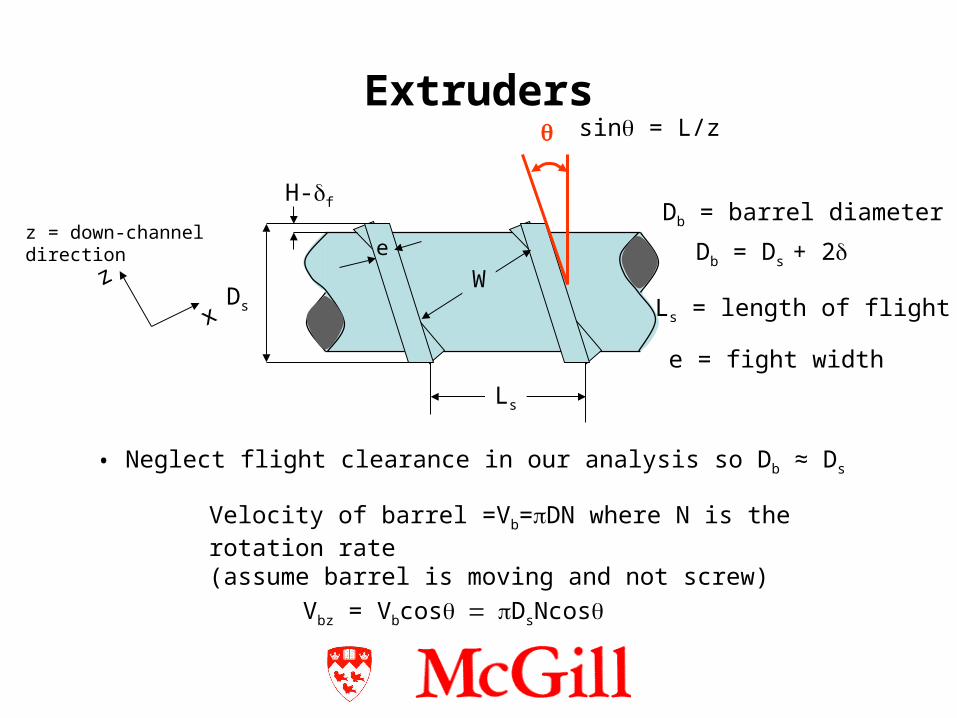
Extruders

Vbz = VbcosDsNcos

• Neglect flight clearance in our analysis so Db ≈ Ds

Velocity of barrel =Vb=DN where N is the rotation rate (assume barrel is moving and not screw)

Ls

W

e

H-f

Ds

Db = Ds + 2

Db = barrel diameter

z

x

z = down-channel direction

Ls = length of flight

e = fight width

sin = L/z

Extruders• Model for fluid

– Newtonian– Apply the flat plate geometry for the case of drag flow and an

opposing pressure flow

dz

dPWHVHWQ

122

1 3

• However, the melt is moving in the “z” down-channel direction

sinsinsin/

coscos

costancos

L

P

dL

dP

Ld

dP

dz

dP

NDVV

DLW

sb

s

Extruders

L

PHDNHDQ s

sextruder

2

322 sin

12cossin

2

1

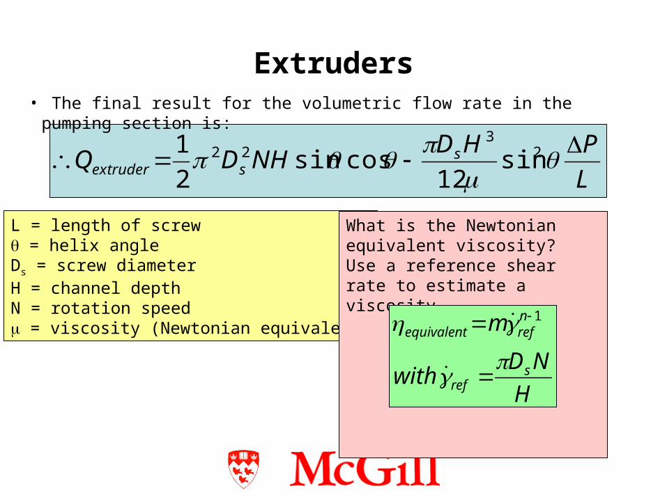
• The final result for the volumetric flow rate in the pumping section is:

L = length of screw = helix angleDs = screw diameterH = channel depthN = rotation speed = viscosity (Newtonian equivalent)

What is the Newtonian equivalent viscosity?Use a reference shear rate to estimate a viscosity.

H

NDwith

m

sref

nrefequivalent

1

Extruders

die

diedie L

PDQ

64

4

• For the volumetric flow rate in the die section for a Newtonian Fluid (Hagen-Poiseuille equation) (assume the die is tubular):

• The expressions for Qdie and Qextruder must be equal. This relationship leads to the operating point for the extruder-die system.

Q

P

operating point

Qmax

extruder

die

Pmax

tan

62

cossin

2max

22

max

H

NLDP

NHDQ

ss

s

Mixing• Extruders (single and twin-screw) are common mixers for polymeric

materials but other mixers used– Static mixers– Roll mills– Batch mixers

• How is mixing characterized?– Uniformity, Texture, Scale, intensity of segregation

• How are mixing processes characterized?– Residence time distribution

• Goal of mixing: Uniform composition

Mixing• Laminar Mixing

– Example: mixing of two viscous liquids.– Interfacial area increases with strain applied.

y

xlinear flow field (eg. drag flow)

vx

At initial time to, the initial area Ao is defined by two vectors 1 and 2:

212

1

2

1 cAo

y

z

x

1

2c

y

z

x

P1 P2

Mixing

A

Ao

cos x

A

Ao

1 2cos x cos y cos2 x2 1/ 2

Ao 1

2cx

2 cy2 cz

2 1/ 2Initially, interfacial area Ao is given by:

At a later time, interfacial area A is given by:

For large deformations,

A 1

2cx

2 cy2 cz

2 2cxcycx22 1/ 2 Note change in position vectors:

x

xyx

ytv

yv

tv

v

v&

Average striation thickness:3

2Lr

L = length of cube side= minor component volume fraction = total strain

Mixing

• Characterization of Mixing– Increase in interfacial area related to strain– Strain distribution function (SDF) describes the strain histories in

a flow field. SDF’s can be determined from velocity distribution

tdtft

yx 0)(

o

o

df

dfF

)(

)()(Cumulative strain distribution function:

Instantaneous strain distribution function:

Mean strain:

Mixing• Example: determine the strain distribution function

(SDF) f()d, the cumulative SDF and the mean strain for drag flow of a Newtonian fluid between parallel plates as shown below.

y

x

Vo

H

L

(Hint: determine the velocity profile and flow rate first)

Mixing

• Besides SDF, the residence time distribution (RTD) function is another important measure of mixing

• Determines time that material spends in the mixer

f (t) E(t)dt dq

qInstantaneous RTD:

Cumulative RTD:

Mean residence time:

F(t) E( t )d t to

t

t tE(t)dtto

Mixing• Example: Determination of the residence time distribution for laminar,

pressure-driven flow in a tube for a Newtonian fluid (see Example 7.8, Tadmor & Gogos)

r

zR

L

(Hint: Given the velocity profile, relate it to the residence time to the given position and the geometry of the tube.)

Mixing • Example: Effect of shear-thinning behavior on strain distribution. Consider a

power-law fluid between two concentric cylinders (Tadmor & Gogos, Example 11.2). Determine the cumulative SDF F(), the SDF f()d and the mean strain and comment on the effect of the power-law parameter “n” on the SDF’s and the mean strain.

Ro

Ri

r

Inner cylinder rotates at constant angular velocity Ω(assuming steady-state, isothermal, laminar flow, no slip and negligible gravity):

ns

R

R

R

r

R

v

i

o

i

ss

ss

i

1;;

122

22

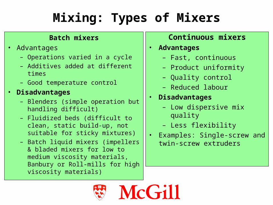
Mixing: Types of Mixers

Batch mixers• Advantages

– Operations varied in a cycle

– Additives added at different times

– Good temperature control

• Disadvantages– Blenders (simple operation but

handling difficult)

– Fluidized beds (difficult to clean, static build-up, not suitable for sticky mixtures)

– Batch liquid mixers (impellers & bladed mixers for low to medium viscosity materials, Banbury or Roll-mills for high viscosity materials)

Continuous mixers• Advantages

– Fast, continuous

– Product uniformity

– Quality control

– Reduced labour

• Disadvantages

– Low dispersive mix quality

– Less flexibility

• Examples: Single-screw and twin-screw extruders

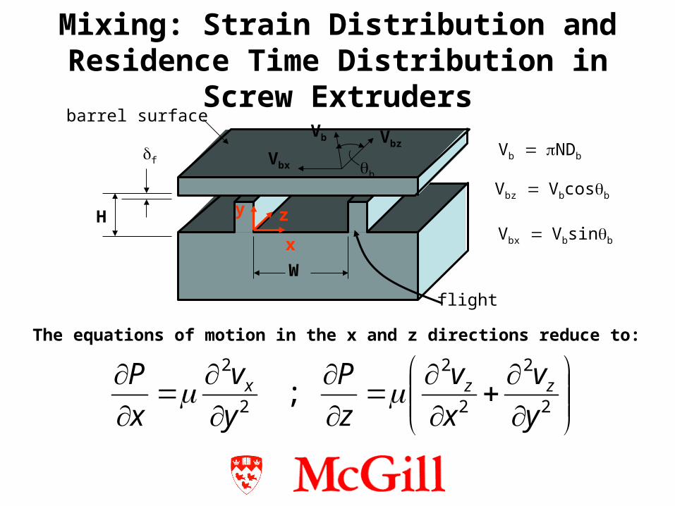
Mixing: Strain Distribution and Residence Time Distribution in Screw Extruders

• Relevant sections: – Baird & Collias, Chapter 8 – Tadmor & Gogos, section 11.10

• Flow is in down-channel direction and is 2-dimensional (vz(x,y)). Barrel surface has velocity component in x-direction to give circulatory flow in the cross-channel direction.

• Assumptions– laminar

– Steady

– Fully-developed

– Isothermal

– Gravity and convection negligible


y

x

z

W

H

f

flight

barrel surfaceVbz

Vbx

Vb

b

Vb NDb

Vbz Vbcosb

Vbx Vbsinb

The equations of motion in the x and z directions reduce to:

2

2

2

2

2

2

;y

v

x

v

z

P

y

v

x

P zzx


2

2 )(),(

y

yv

x

zxP x

• Since both sides of the equation of motion in the x-direction are independent of each other, vx can be determined by integration subject to the following boundary conditions:

1) vx(0) = 02) vx(H) = -Vbx.

The velocity profile is:

H

yand

V

vuwhere

x

P

V

Hu

bx

xx

bxx

21

2


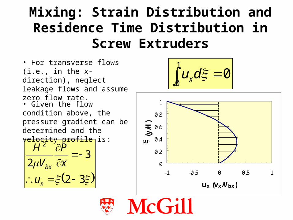
01

0 dux

32

32

2

x

bx

u

x

P

V

H

• For transverse flows (i.e., in the x-direction), neglect leakage flows and assume zero flow rate.

• Given the flow condition above, the pressure gradient can be determined and the velocity profile is:

0

0.2

0.4

0.6

0.8

1

-1 -0.5 0 0.5 1

ux (vx/Vbx)

(y

/H)


• For flow in the down-channel direction (i.e. z-direction), the equation of motion in the z-direction is solved by separation of variables subject to the following boundary conditions:

0),(

0),0(

),(

0)0,(

2

2

2

2

yWv

yv

VHxv

xv

y

v

x

v

z

P

z

z

bzz

z

zz


• The velocity profile in the z-direction is given by the following equation (see Tadmor and Klein, “Engineering Principles of Plasticating Extrusion”, Van Nostrand, NY, (1970), p. 194).

i

hih

ii

z

P

V

H

ihii

hiu

ibz

iz

sin

2cosh

5.0cosh8

2

sinsinh

sinh4

5,3,1

3

32

2

5,3,1

where uz=vz/Vbz, = x/W and h = H/W.


• As in the cross-channel direction, the velocity profile can be integrated to give the volumetric flow rate in the down-channel direction and the pressure gradient can be determined.

1

0

1

0

dduWHVQ zbz

5,3,155

5,3,133

3

2tanh

11921

2tanh

116

122

ip

idpd

bz

H

Wi

iW

HFand

W

Hi

iH

WFwhereF

z

PWHF

WHVQ

drag flow pressure flow

QpQd

Fp and Fd are “shape factors” for pressure and drag flow


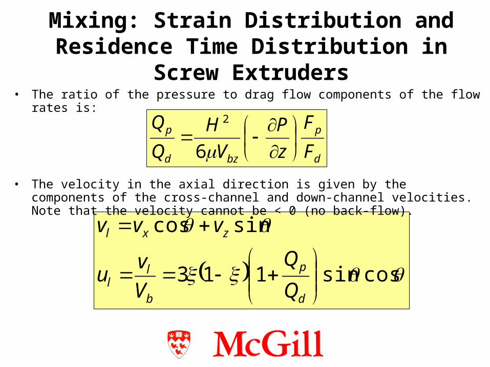
• The ratio of the pressure to drag flow components of the flow rates is:

d

p

bzd

p

F

F

z

P

V

H

Q

Q

6

2

cossin113

sincos

d

p

b

ll

zxl

Q

Q

V

vu

vvv

• The velocity in the axial direction is given by the components of the cross-channel and down-channel velocities. Note that the velocity cannot be < 0 (no back-flow).


Velocity profiles in cross-channel, down-channel and axial directions for various Qp/Qd values in shallow, square pitched screws (i.e. = 17.65o)

0

0.2

0.4

0.6

0.8

1

-0.4 -0.2 0 0.2

vx/Vb

e (y/H)

0

0.2

0.4

0.6

0.8

1

-0.4 -0.2 0 0.2 0.4 0.6 0.8 1

vz/Vb

e(y/H)

0

0.2

0.4

0.6

0.8

1

0 0.2 0.4

vl/Vb

e (y/H)

0

0.2

0.4

0.6

0.8

1

-0.4 -0.2 0 0.2

vx/Vb

e (y/H)

0

0.2

0.4

0.6

0.8

1

-0.4 -0.2 0 0.2 0.4 0.6 0.8 1

vz/Vb

e(y/H)

0

0.2

0.4

0.6

0.8

1

0 0.2 0.4

vl/Vb

e (y/H)

Qp/Qd = 0

Qp/Qd = -1/3

Mixing in Extruders (Cont.)

0

0.2

0.4

0.6

0.8

1

-0.4 -0.2 0 0.2

vx/Vb

e (y/H)

0

0.2

0.4

0.6

0.8

1

-0.4 -0.2 0 0.2 0.4 0.6 0.8 1

vz/Vb

e(y/H)

0

0.2

0.4

0.6

0.8

1

0 0.2 0.4

vl/Vb

e (y/H)

0

0.2

0.4

0.6

0.8

1

-0.4 -0.2 0 0.2

vx/Vb

e (y/H)

0

0.2

0.4

0.6

0.8

1

-0.4 -0.2 0 0.2 0.4 0.6 0.8 1

vz/Vb

e(y/H)

Qp/Qd = -2/3

Qp/Qd = -10

0.2

0.4

0.6

0.8

1

0 0.2 0.4

vl/Vb

e (y/H)

Residence Time Distributions in Extruders• Operating conditions, melt viscosity and channel depth affect down-

channel but not cross-channel velocity profile• Particle in x-direction re-circulates in upper part of channel (see Fig.

11.27 & 11.28 in Tadmor and Gogos). This is described as follows:

1,3211

2

1

0,32112

1

322

322

1

0

c

cccc

xx duduc

Valid for shallow channels but ignores leakage flows, non-Newtonian effects, thermal effects and flight geometry

Residence Time Distributions in Extruders

xbx uV

W

Fraction of time fluid particle spends in upper part of the channel:

Residence time of fluid particle in upper part of channel:

Residence time of fluid particle in lower part of channel:

cxbx uV

W

ccxbxcxbx

cxbxf

uVW

uVW

uVW

t

3232

1

1


t l

Vbu l l

Vb ul t f ul c 1 t f

t l

3Vb 1Qp

Qd

sin cos

3 1 3 12 32

1 12 32

The axial residence time is given by:

The minimum residence time occurs when ux = 0 ( = 2/3):

t0 3l

2Vb 1Qp

Qd

sin cos


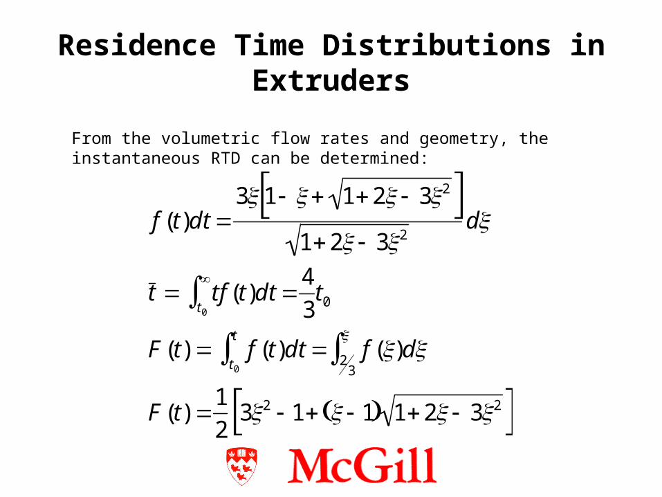
f (t)dt 3 1 12 32

12 32d

t tf (t)dt 4

3t0

t0

F(t) f (t)dt t0

t f ()d2

3

F(t) 12

32 1 1 12 32

From the volumetric flow rates and geometry, the instantaneous RTD can be determined:

Polymer Blends

• Most polymers are sold as blends (> 30%; Utracki et al)• Why blend polymers

– More economic than making a new polymer– Combine synergistic properties– Reduce cost of base material

• Commercial blends available– HIPS (Shell) (poly(styrene)/poly(butadiene))– Nylon ST (DuPont) (nylon/(ethylene-propylene) copolymer

rubber)– Xenoy (General Electric) (poly(phenyleneoxide)/poly(styrene))

Polymer Blends• Consider mixing of liquid-liquid dispersions in Newtonian systems

– Taylor (1934) examined break-up of a single Newtonian drop in a Newtonian matrix

5.2;

44

1914

r

rm

rD

L

B

shear field

BL

B - L n deformatio

m

dr

d

m

ratioviscosity

viscosityphase dispersed

viscositymatrix

rateshear

tensionlinterfacia

diameterdropstablemaximumD

Polymer Blends• Consider mixing of liquid-liquid dispersions in viscoelastic systems

– Wu (1982) related drop size to rheological and interfacial properties using a semi-empirical relation for concentrated, non-Newtonian polymeric fluids

1-s 100 rate shear effective and ionconcentrat

phase dispersed wt%15 withblends forstrictly Applies

forexponentinsign minus

forexponentinsign plus

1)(

1

;4 84.0

r

r

m

rD

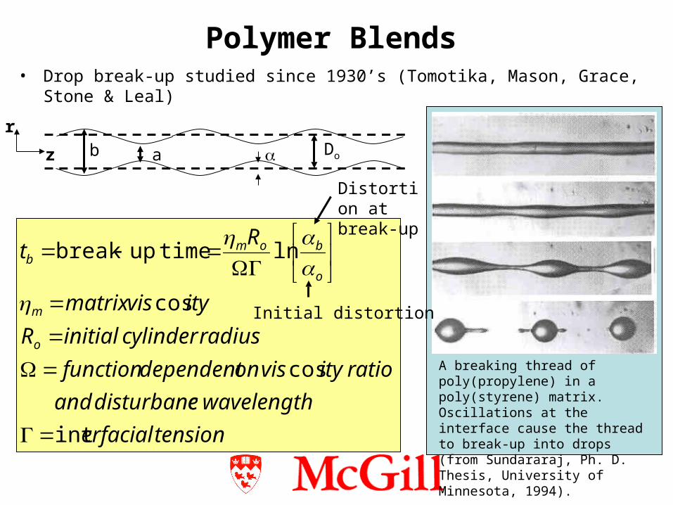
Polymer Blends• Drop break-up studied since 1930’s (Tomotika, Mason, Grace, Stone & Leal)

A breaking thread of poly(propylene) in a poly(styrene) matrix. Oscillations at the interface cause the thread to break-up into drops (from Sundararaj, Ph. D. Thesis, University of Minnesota, 1994).

Doa b

r

z

tensionerfacial

wavelengthedisturbancand

ratioityvisondependentfunction

radiuscylinderinitialR

ityvismatrix

Rt

o

m

o

bomb

int

cos

cos

ln

timeupbreak

Distortion at break-up

Initial distortion

Polymer Blends

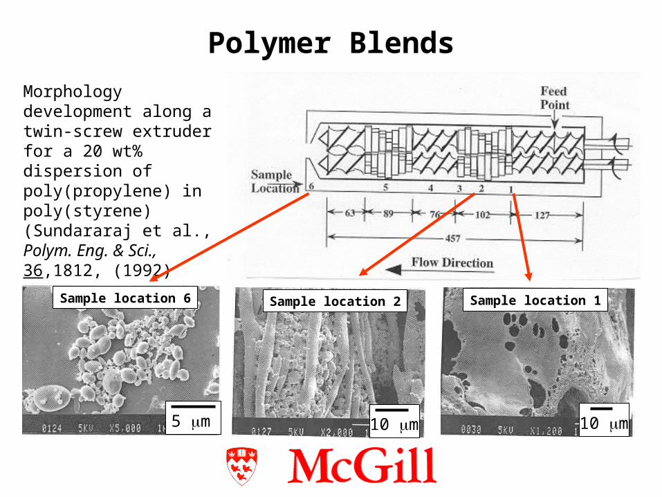
Morphology development along a twin-screw extruder for a 20 wt% dispersion of poly(propylene) in poly(styrene) (Sundararaj et al., Polym. Eng. & Sci., 36,1812, (1992)

Fig10 Macosko et al Macro 1996.htm

10 m

Sample location 1

10 m

Sample location 2

5 m

Sample location 6

• Morphology development in polymer blends (Macosko et al, Macromolecules, 29, 5590, (1996)).

Fig10 Macosko et al Macro 1996.htm

Polymer Blends

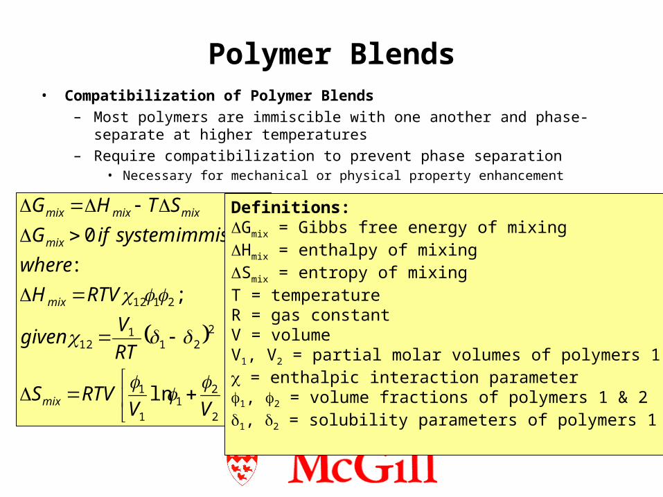
Polymer Blends• Compatibilization of Polymer Blends

– Most polymers are immiscible with one another and phase-separate at higher temperatures

– Require compatibilization to prevent phase separation• Necessary for mechanical or physical property enhancement

22

21

1

1

221

112

2112

lnln

;

:

0

VVRTVS

RT

Vgiven

RTVH

where

immisciblesystemifG

STHG

mix

mix

mix

mixmixmix Definitions:Gmix = Gibbs free energy of mixingHmix = enthalpy of mixingSmix = entropy of mixingT = temperatureR = gas constantV = volumeV1, V2 = partial molar volumes of polymers 1 & 2 = enthalpic interaction parameter1, 2 = volume fractions of polymers 1 & 21, 2 = solubility parameters of polymers 1 & 2

Polymer Blends• Methods to compatibilize polymer

blends– Pre-made block copolymer

addition– Reactive blending

Magnify interface

Reactive blending

B

BAA

B A

pre-made block copolymer addition

Advantages• Copolymer formed at interfaceDisadvantages• Functionalizing homopolymers

Advantages• small amount requiredDisadvantages• micelles• slow copolymer diffusion rate to interface

Polymer A Polymer B

Functional groups A + B react at interface

Block copolymer micelle

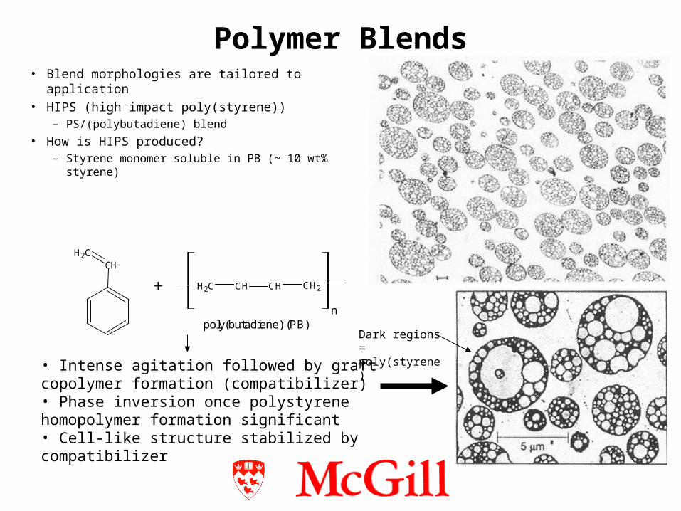
Polymer Blends• Blend morphologies are tailored to application• HIPS (high impact poly(styrene))

– PS/(polybutadiene) blend

• How is HIPS produced?– Styrene monomer soluble in PB (~ 10 wt% styrene)

CHCH2

CH2 CH CH CH2

npoly(butadiene) (PB)

+

• Intense agitation followed by graft copolymer formation (compatibilizer)• Phase inversion once polystyrene homopolymer formation significant• Cell-like structure stabilized by compatibilizer

Dark regions = poly(styrene)

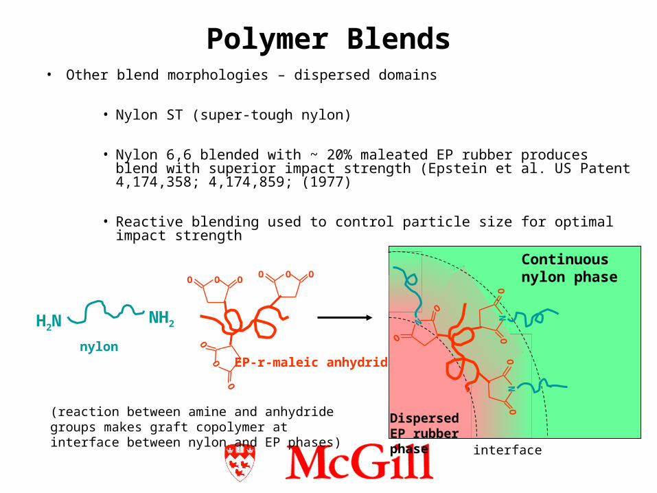
Polymer Blends• Other blend morphologies – dispersed domains

• Nylon ST (super-tough nylon)

• Nylon 6,6 blended with ~ 20% maleated EP rubber produces blend with superior impact strength (Epstein et al. US Patent 4,174,358; 4,174,859; (1977)

• Reactive blending used to control particle size for optimal impact strength

(reaction between amine and anhydride groups makes graft copolymer at interface between nylon and EP phases)

OO OOO O

O

O

O

NH2H2N

nylonEP-r-maleic anhydride

Dispersed EP rubber phase

Continuous nylon phase

NO

ON

OO

N

O

O

interface

Polymer Blends

Taken from Gonzalez-Montiel et al. Polymer, 24, 4587, (1995).

• Rubber toughened nylons can have morphology controlled by varying level of reaction

• Many examples in literature – see adjacent figure for example

• All blends in figure are 80 wt% nylon 6 with 20 wt % dispersed poly(propylene) (PP) phase)

• Nylon 6 stained dark in micrographs; PP is white

• More reactive rubber added, finer dispersion of EP in nylon

5 m

10% EPMAno EPMA

15% EPMA 25% EPMA

5 m

5 m 5 m

chemical engineering 584: polymer processing lecture 7: extrusion and mixing

Documents