che 494/598, eee 598 intro to system identification ... · estimation and validation, march 26,...

© Copyright 1997, 1998 by D.E. Rivera, All Rights Reserved

ChE 494/598, EEE 598 Intro to System Identification: Parametric Model Estimation and Validation, March 26, 1998

1

Daniel E. Rivera, Associate Professor

Department of Chemical, Bio and Materials Engineeringand

Control Systems Engineering LaboratoryArizona State UniversityTempe AZ 85287-6006

[email protected], (602) 965-9476© Copyright, 1997, 1998

System Identification for Process Control:A Short Course: Module Three

Course Outline

• Closed-Loop Identification

• Signals and Systems Overview

• Input Signal Design and Nonparametric Estimation

• Module 3: Parametric Model Estimation and Validation

• Control-Relevant Identification

• Multivariable Identification

Today's OutlineLECTURE:

• Prediction-Error (Parametric) Estimation Techniques

• Classical Model Validation Techniques

• "Hairdryer" data example

LAB:

• Illustration of System ID Toolbox Graphical Interface

• Simulated Fifth-order System Laboratory #2

• Phenol Plant Data Lab #2

STAGES OF SYSTEM IDENTIFICATION

Start

Experimental Design and Execution

"ID Packages"

Model Validation

Does the model meet validation criteria?

( Step, Pulse, or PRBS-Generated Data)

( Linear Plant and Disturbance Models)

(Simulation, Residual auto and crosscorrelation,step-response)

No

End

Yes

a priori processinformation

• Model Structure Determination

• Parameter Estimation

• Data Preprocessing



2

Smoothing, Filtering, Prediction

• In the prediction problem, current and previous measurements from the plant are used to obtain estimates k+1 (or beyond) time steps in the future

Prediction-Error Model Structures

Some general info

• Use of regression techniques to get a model estimate

• Regression may be linear or nonlinear, depending on the model structure

• 32 general formulations for prediction-error models, of which only five are commonly used

System Identification Problem

noise signal (usually assumed white)

Input Signal (Random orDeterministic)

Output Signal (random, autocorrelated)

u

yP(z)

a

++

H(z)

υDisturbance Signal (random, autocorrelated)

True Plant: y(t) = p(z)u(t) +H(z)a(t)Plant Model: y(t) = p(z)u(t) + pe(z)e(t)

A(z)y(t) =B(z)F (z)

u(t− nk) +C(z)D(z)

e(t)

A(z) = 1 + a1z−1 + . . .+ anaz

−na

B(z) = b1 + b2z−1 + . . .+ bnbz

−nb+1

C(z) = 1 + c1z−1 + . . .+ cncz

−nc

D(z) = 1 + d1z−1 + . . .+ dndz

−nd

F (z) = 1 + f1z−1 + . . .+ fnfz

−nf

In transfer function form:

y(t) = p(z)u(t) + pe(z)e(t)

p(z) =B(z)

A(z)F (z)z−nk pe(z) =

C(z)A(z)D(z)

Prediction-Error Model Structures

C(z)D(z)

1A(z)

e

yu B(z)F(z)

−nkz ++

Prediction-Error Family of Models



3

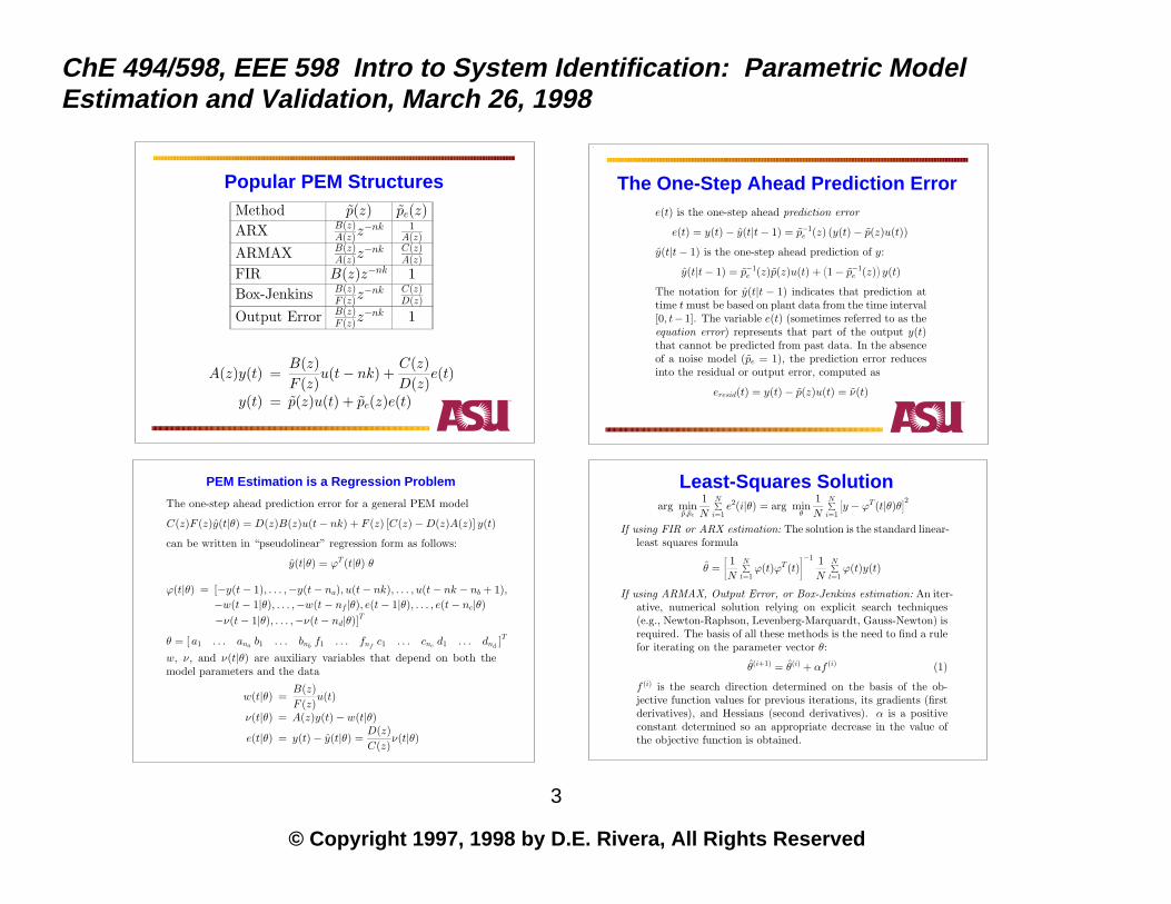
Popular PEM StructuresMethod p(z) pe(z)ARX B(z)

A(z)z−nk 1

A(z)

ARMAX B(z)A(z)z

−nk C(z)A(z)

FIR B(z)z−nk 1Box-Jenkins B(z)

F (z)z−nk C(z)

D(z)

Output Error B(z)F (z)z

−nk 1

A(z)y(t) =B(z)F (z)


e(t)

y(t) = p(z)u(t) + pe(z)e(t)

The One-Step Ahead Prediction Errore(t) is the one-step ahead prediction error

e(t) = y(t)− y(t|t− 1) = p−1e (z) (y(t)− p(z)u(t))

y(t|t− 1) is the one-step ahead prediction of y:

y(t|t− 1) = p−1e (z)p(z)u(t) +

(1− p−1

e (z))y(t)

The notation for y(t|t − 1) indicates that prediction attime t must be based on plant data from the time interval[0, t−1]. The variable e(t) (sometimes referred to as theequation error) represents that part of the output y(t)that cannot be predicted from past data. In the absenceof a noise model (pe = 1), the prediction error reducesinto the residual or output error, computed as

eresid(t) = y(t)− p(z)u(t) = ν(t)

The one-step ahead prediction error for a general PEM model

C(z)F (z)y(t|θ) = D(z)B(z)u(t− nk) + F (z) [C(z)−D(z)A(z)] y(t)

can be written in “pseudolinear” regression form as follows:

y(t|θ) = ϕT (t|θ) θ

ϕ(t|θ) = [−y(t− 1), . . . ,−y(t− na), u(t− nk), . . . , u(t− nk − nb + 1),−w(t− 1|θ), . . . ,−w(t− nf |θ), e(t− 1|θ), . . . , e(t− nc|θ)−ν(t− 1|θ), . . . ,−ν(t− nd|θ)]T

θ = [ a1 . . . ana b1 . . . bnb f1 . . . fnf c1 . . . cnc d1 . . . dnd ]T

w, ν, and ν(t|θ) are auxiliary variables that depend on both themodel parameters and the data

w(t|θ) =B(z)F (z)

u(t)

ν(t|θ) = A(z)y(t)− w(t|θ)

e(t|θ) = y(t)− y(t|θ) =D(z)C(z)

ν(t|θ)

PEM Estimation is a Regression Problem Least-Squares Solutionarg min

p,pe

1N

N∑i=1e2(i|θ) = arg min

θ

1N

N∑i=1

[y − ϕT (t|θ)θ

]2

If using FIR or ARX estimation: The solution is the standard linear-least squares formula

θ = 1N

N∑t=1

ϕ(t)ϕT (t)−1 1N

N∑t=1

ϕ(t)y(t)

If using ARMAX, Output Error, or Box-Jenkins estimation: An iter-ative, numerical solution relying on explicit search techniques(e.g., Newton-Raphson, Levenberg-Marquardt, Gauss-Newton) isrequired. The basis of all these methods is the need to find a rulefor iterating on the parameter vector θ:

θ(i+1) = θ(i) + αf (i) (1)

f (i) is the search direction determined on the basis of the ob-jective function values for previous iterations, its gradients (firstderivatives), and Hessians (second derivatives). α is a positiveconstant determined so an appropriate decrease in the value ofthe objective function is obtained.



4

AutoRegressive with eXternal input structure (ARX)

A(z)y(t) = B(z)u(t− nk) + e(t)

A(z) = 1 + a1z−1 + . . .+ anaz

−na

B(z) = b1 + b2z−1 + . . .+ bnbz

−nb+1

• Estimation problem involves a linear regression problem.

• High-order ARX estimation (na and nb large) yields consistent estimates but may result in variance problems in the presence of significant noise.

• Low-order ARX estimation is problematic 1) in the presence of significant noise and 2) when an incorrect model structure is chosen.

ARX Parameter EstimationThe one-step ahead predictor for y

y(t|t−1) = −a1y(t−1)−. . .−anay(t−na)+b1u(t−nk)+. . .+bnbu(t−nk−nb+1)

can be expressed as a linear regression problem via

ϕ = [−y(t− 1) . . . −y(t− na) u(t− nk) . . . u(t− nk − nb + 1) ]T

and θ, the vector of parameter estimates:

θ = [ a1 . . . ana b1 . . . bnb ]T

Rewriting the objective (“loss”) function as

minθV = min

θ

1N

N∑i=1

[y − ϕT (t)θ

]2

leads to the well-established linear least-squares solution

θ = 1N

N∑t=1

ϕ(t)ϕT (t)−1 1N

N∑t=1

ϕ(t)y(t)

AutoRegressive Moving Average with eXternal input structure (ARMAX)A(z)y(t) = B(z)u(t− nk) + C(z)e(t)

A(z) = 1 + a1z−1 + . . .+ anaz

−na

B(z) = b1 + b2z−1 + . . .+ bnbz

−nb+1

C(z) = 1 + c1z−1 + . . .+ cncz

−nc

• Estimation problem is a nonlinear regression problem

• Model orders (na, nb, nc) usually chosen to be low.

• Presence of autoregressive polynomial can yield bias problems in the presence of significant noise and/or model structure mismatch; moving average polynomial will sometimes counteract negative effects, however.

Finite Impulse Response (FIR)

y(t) = B(z)u(t− nk) + e(t)B(z) = b1 + b2z

−1 + . . .+ bnbz−nb+1

• "Structure-free" model representation equivalent to what we saw in correlation analysis

• Estimation problem is linear regression problem

• Because of fast sampling, model order (nb) is usually high (20 coefficients or more)

• No autocorrelated noise model is estimated.



5

Box-Jenkins (B-J) Model Structure

y(t) =B(z)F (z)


e(t)

B(z) = b1 + b2z−1 + . . .+ bnbz

−nb+1

C(z) = 1 + c1z−1 + . . .+ cncz

−nc

D(z) = 1 + d1z−1 + . . .+ dndz

−nd

F (z) = 1 + f1z−1 + . . .+ fnfz

−nf

• Estimation problem is a nonlinear regression problem

• Model orders (nb, nc, nd, nf) usually chosen to be low.

• Independently parametrizes transfer function and noise models; lots of decisions and possibly many iterations to be made by the user, however.

Output Error (OE) Model Structure

y(t) =B(z)F (z)

u(t− nk) + e(t)

B(z) = b1 + b2z−1 + . . .+ bnbz

−nb+1

F (z) = 1 + f1z−1 + . . .+ fnfz

−nf

• Estimation problem a nonlinear regression problem

• Model orders (nb, nf) usually chosen to be low.

• Independently parametrizes the input and noise, although an autocorrelated noise model is not obtained.

• Works great in conjunction with control-relevant prefiltering

Represent the ZOH first-order delay model using the five PEM structures (assume a noise-free situation):

Kτs +1

exp(−θs) θ = NT( )

Selecting a "Suitable" Model Structure

K(1 - exp(-T/τ))z-Nz - exp(-T/τ)

ARX: na = 1, nb = 1, nk = N + 1 ARMAX: na = 1, nb = 1, nc = Not Applicable, nk = N + 1

FIR: nb > 3*tau/T, nk = N + 1, (model must capture at least 95% settling time)

Box-Jenkins: nb = 1, nf = 1, nc = NA, nd = NA, nk = N+1

Output Error: nb = 1, nf = 1, nk = N+1

Principal Sources of Error in System Identification

• BIAS. Systematic errors caused by

- input signal characteristics (i.e., excitation) - choice of model structure

- mode of operation (i.e., closed-loop instead of open-loop)

• VARIANCE. Random errors introduced by the presence of noise in the data, which do not allow the model to exactly reproduce the plant output. It is affected by the following factors:

- number of model parameters

- duration of the identification test

- signal-to-noise ratio

ERROR = BIAS + VARIANCE



6

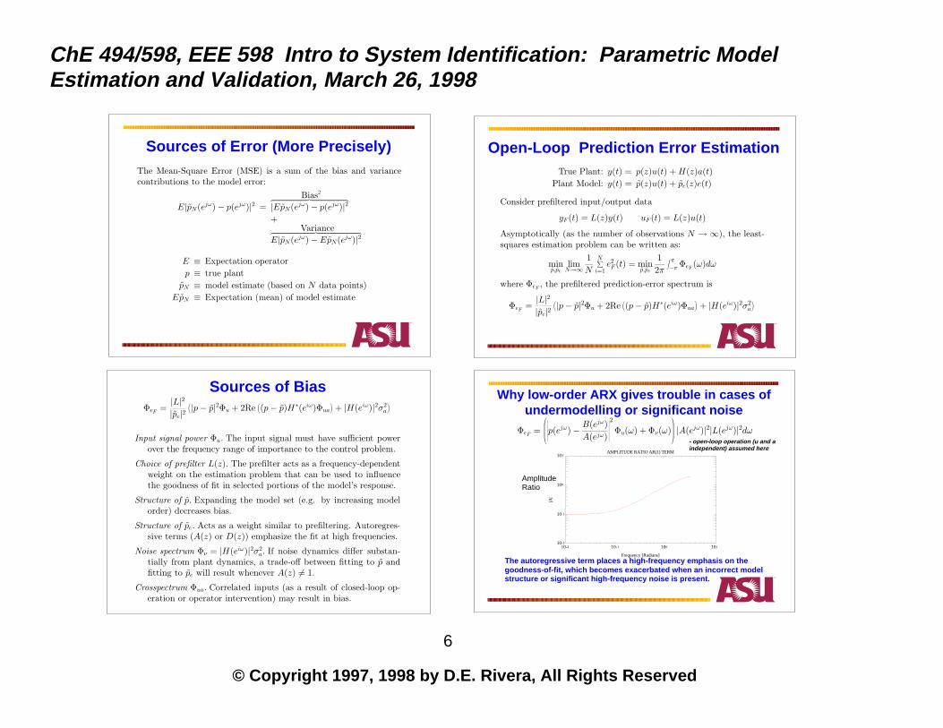
Sources of Error (More Precisely)The Mean-Square Error (MSE) is a sum of the bias and variancecontributions to the model error:

E|pN(ejω)− p(ejω)|2 =Bias2︷︸︸︷

|EpN(ejω)− p(ejω)|2+

Variance︷︸︸︷E|pN(ejω)− EpN(ejω)|2

E ≡ Expectation operatorp ≡ true plant

pN ≡ model estimate (based on N data points)EpN ≡ Expectation (mean) of model estimate

Open-Loop Prediction Error EstimationTrue Plant: y(t) = p(z)u(t) +H(z)a(t)

Plant Model: y(t) = p(z)u(t) + pe(z)e(t)

Consider prefiltered input/output data

yF (t) = L(z)y(t) uF (t) = L(z)u(t)

Asymptotically (as the number of observations N → ∞), the least-squares estimation problem can be written as:

minp,pe

limN→∞

1N

N∑i=1e2F (t) = min

p,pe

12π

∫ π−π ΦeF (ω)dω

where ΦeF , the prefiltered prediction-error spectrum is

ΦeF =|L|2|pe|2

(|p− p|2Φu + 2Re

((p− p)H∗(eiω)Φua

)+ |H(eiω)|2σ2

a

)

Sources of BiasΦeF =

|L|2|pe|2

(|p− p|2Φu + 2Re


)+ |H(eiω)|2σ2

a

)

Input signal power Φu. The input signal must have sufficient powerover the frequency range of importance to the control problem.

Choice of prefilter L(z). The prefilter acts as a frequency-dependentweight on the estimation problem that can be used to influencethe goodness of fit in selected portions of the model’s response.

Structure of p. Expanding the model set (e.g. by increasing modelorder) decreases bias.

Structure of pe. Acts as a weight similar to prefiltering. Autoregres-sive terms (A(z) or D(z)) emphasize the fit at high frequencies.

Noise spectrum Φν = |H(eiω)|2σ2a. If noise dynamics differ substan-

tially from plant dynamics, a trade-off between fitting to p andfitting to pe will result whenever A(z) 6= 1.

Crosspectrum Φua. Correlated inputs (as a result of closed-loop op-eration or operator intervention) may result in bias.

Why low-order ARX gives trouble in cases of undermodelling or significant noise

10-2

10-1

100

101

10-2 10-1 100 101

Frequency [Radians]

|A|

AMPLITUDE RATIO AR(1) TERM

ΦeF =

∣∣∣∣∣∣∣∣p(e

jω)− B(ejω)A(ejω)

∣∣∣∣∣∣∣∣2

Φu(ω) + Φν(ω)

|A(ejω)|2|L(ejω)|2dω

Amplitude Ratio

- open-loop operation (u and a independent) assumed here

The autoregressive term places a high-frequency emphasis on the goodness-of-fit, which becomes exacerbated when an incorrect model structure or significant high-frequency noise is present.



7

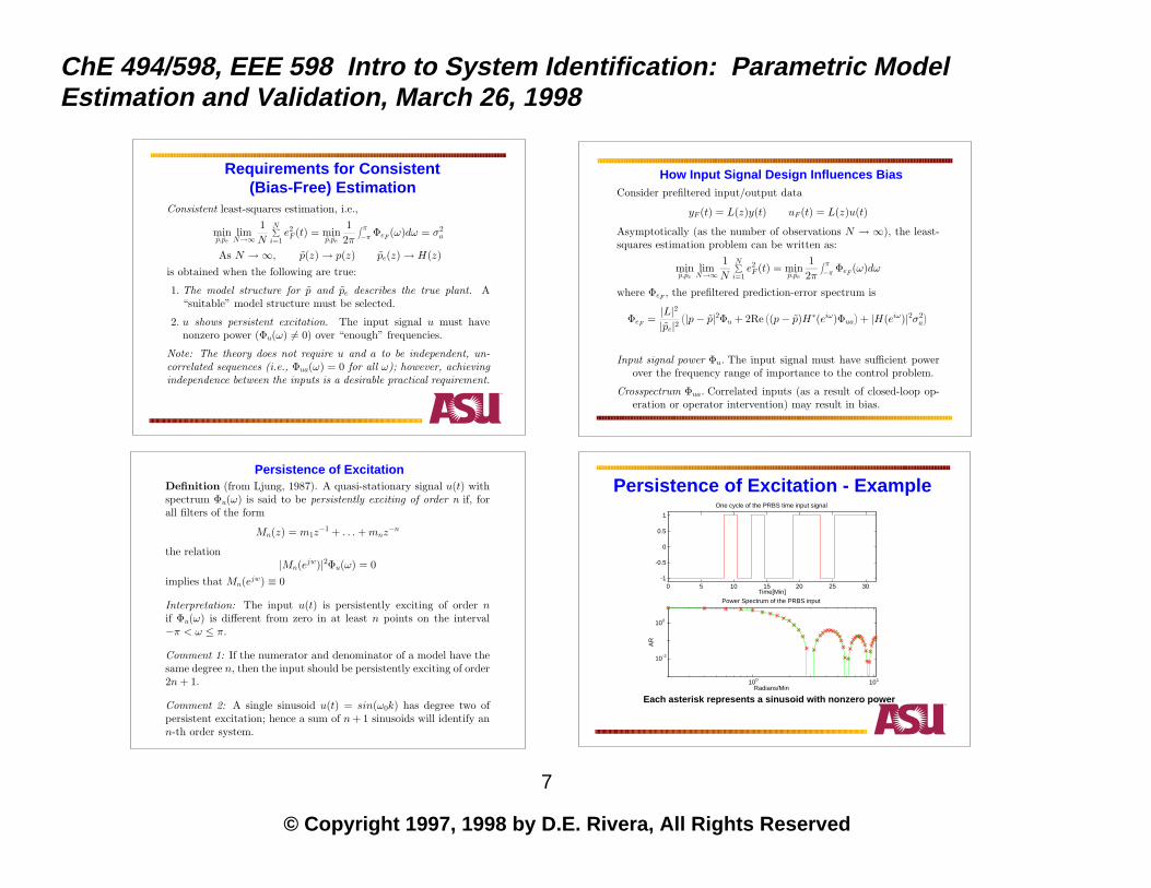
Requirements for Consistent (Bias-Free) Estimation

Consistent least-squares estimation, i.e.,

minp,pe

limN→∞

1N


p,pe

12π

∫ π−π ΦeF (ω)dω = σ2

a

As N →∞, p(z)→ p(z) pe(z)→ H(z)is obtained when the following are true:

1. The model structure for p and pe describes the true plant. A“suitable” model structure must be selected.

2. u shows persistent excitation. The input signal u must havenonzero power (Φu(ω) 6= 0) over “enough” frequencies.

Note: The theory does not require u and a to be independent, un-correlated sequences (i.e., Φua(ω) = 0 for all ω); however, achievingindependence between the inputs is a desirable practical requirement.

How Input Signal Design Influences BiasConsider prefiltered input/output data

yF (t) = L(z)y(t) uF (t) = L(z)u(t)

Asymptotically (as the number of observations N → ∞), the least-squares estimation problem can be written as:

minp,pe

limN→∞

1N


p,pe

12π

∫ π−π ΦeF (ω)dω

where ΦeF , the prefiltered prediction-error spectrum is

ΦeF =|L|2|pe|2

(|p− p|2Φu + 2Re


)+ |H(eiω)|2σ2

a

)

Input signal power Φu. The input signal must have sufficient powerover the frequency range of importance to the control problem.

Crosspectrum Φua. Correlated inputs (as a result of closed-loop op-eration or operator intervention) may result in bias.

Persistence of ExcitationDefinition (from Ljung, 1987). A quasi-stationary signal u(t) withspectrum Φu(ω) is said to be persistently exciting of order n if, forall filters of the form

Mn(z) = m1z−1 + . . .+mnz

−n

the relation|Mn(ejw)|2Φu(ω) = 0

implies that Mn(ejw) ≡ 0

Interpretation: The input u(t) is persistently exciting of order nif Φu(ω) is different from zero in at least n points on the interval−π < ω ≤ π.

Comment 1: If the numerator and denominator of a model have thesame degree n, then the input should be persistently exciting of order2n+ 1.

Comment 2: A single sinusoid u(t) = sin(ω0k) has degree two ofpersistent excitation; hence a sum of n+ 1 sinusoids will identify ann-th order system.

Persistence of Excitation - Example

0 5 10 15 20 25 30-1

-0.5

0

0.5

1

One cycle of the PRBS time input signal

Time[Min]

100 101

10-2

100

Radians/Min

AR

Power Spectrum of the PRBS input

Each asterisk represents a sinusoid with nonzero power



8

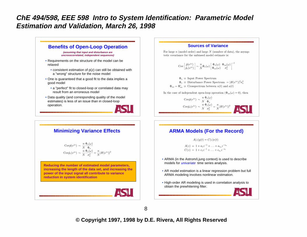
Benefits of Open-Loop Operation(assuming that input and disturbance are

uncrosscorrelated, independent sequences)

• Requirements on the structure of the model can be relaxed

• consistent estimation of p(z) can still be obtained with a "wrong" structure for the noise model

• One is guaranteed that a good fit to the data implies a good model

• a "perfect" fit to closed-loop or correlated data may result from an erroneous model

• Data quality (and corresponding quality of the model estimates) is less of an issue than in closed-loop operation.

Sources of VarianceFor large n (model order) and large N (number of data), the asymp-totic covariance for the unbiased model estimate is:

Cov p(e

jω)pe(ejω)

∼ n

NΦν(ω)

Φu(ω) Φua(ω)Φau(ω) σ2

a

−1

Φu ≡ Input Power SpectrumΦν ≡ Disturbance Power Spectrum = |H(eiω)|2σ2

a

Φua = Φ∗au ≡ Crosspectrum between u(t) and a(t)

In the case of independent open-loop operation (Φua(ω) = 0), then

Covp(ejω) ∼ n

N

Φν(ω)Φu

Covpe(ejω) ∼ n

N

Φν(ω)σ2a

=n

N|H(eiω)|2

Reducing the number of estimated model parameters,increasing the length of the data set, and increasing the power of the input signal all contribute to variance reduction in system identification

Minimizing Variance Effects

Covp(ejω) ∼ n

N

Φν(ω)Φu

Covpe(ejω) ∼ n

N

Φν(ω)σ2a

=n

N|H(eiω)|2

ARMA Models (For the Record)

A(z)y(t) = C(z)e(t)

A(z) = 1 + a1z−1 + . . .+ anaz

−na

C(z) = 1 + c1z−1 + . . .+ cncz

−nc

• ARMA (in the Astrom/Ljung context) is used to describe models for univariate time series analysis.

• AR model estimation is a linear regression problem but full ARMA modeling involves nonlinear estimation.

• High-order AR modeling is used in correlation analysis to obtain the prewhitening filter.



9

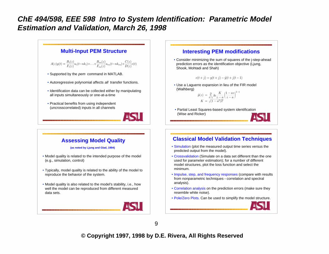
Multi-Input PEM Structure

A(z)y(t) =B1(z)F1(z)

u1(t−nk1)+. . .+Bnu(z)Fnu(z)

unu(t−nknu)+C(z)D(z)

e(t)

• Identification data can be collected either by manipulating all inputs simultaneously or one-at-a-time

• Practical benefits from using independent (uncrosscorrelated) inputs in all channels

• Supported by the pem command in MATLAB.

• Autoregressive polynomial affects all transfer functions.

Interesting PEM modifications• Consider minimizing the sum of squares of the j-step-ahead

prediction errors as the identification objective (Ljung, Shook, Mohtadi and Shah)

e(t+ j) = y(t+ j)− y(t+ j|t− 1)

• Use a Laguerre expansion in lieu of the FIR model (Walhberg)

p(z) =∞∑k=1

gkK

z − a

1− azz − a

k−1

K =√(1− a2)T

• Partial Least Squares-based system identification (Wise and Ricker)

Assessing Model Quality(as noted by Ljung and Glad, 1994)

• Model quality is related to the intended purpose of the model (e.g., simulation, control)

• Typically, model quality is related to the ability of the model to reproduce the behavior of the system.

• Model quality is also related to the model's stability, i.e., how well the model can be reproduced from different measured data sets.

Classical Model Validation Techniques• Simulation (plot the measured output time series versus the

predicted output from the model).

• Crossvalidation (Simulate on a data set different than the one used for parameter estimation); for a number of different model structures, plot the loss function and select the minimum.

• Impulse, step, and frequency responses (compare with results from nonparametric techniques - correlation and spectral analysis).

• Correlation analysis on the prediction errors (make sure they resemble white noise).

• Pole/Zero Plots. Can be used to simplify the model structure.



10

Information CriteriaIn the absence of crossvalidation data, these criteria can be used tobalance between model fit and the number of parameters used.

Akaike’s information criterion (AIC):

mind,θ

(1 +2dN

)N∑i=1e2(t, θ)

Final Prediction Error (FPE):

mind,θ

1 + d/N

1− d/N1N

N∑i=1e2(t, θ)

Rissanen’s minimal description length (MDL):

mind,θ

(1 +2dN· logN)

N∑i=1e2(t, θ)

N ≡ Data lengthθ ≡ Vector of parameter estimatesd = dim θ (no. of estimated parameters)

e(t, θ) ≡ One-step-ahead prediction error for a given θ

Prediction-Error Correlation Analysis

e(t) = p−1e (z) ((p(z)− p(z))u(t) +H(z)a(t))

Autocorrelation in e:

ρe(k) =γe(k)σ2e

Cross-correlation between e and u:

ρue(k) =γue(k)√σ2uσ

2e

• autocorrelation in the residuals means that the noise model structure is incorrect.

• crosscorrelation between the residuals and the input signifies undermodelling, the input/output model structure is incorrect.

Feedback's Process Trainer PT326

• "Hairdryer" process; input (MV) is the voltage over the heating device; output (CV) is outlet temperature

% ARX estimation% th = arx([y u],[na nb nk]) th = arx(z2,[1 1 1]);th = sett(th,0.08); % Set the correct sampling interval.

pause, present(th) % Press any key to see model.This matrix was created by the command ARX on 6/23 1994 at 21:22Loss fcn: 0.03657 Akaike`s FPE: 0.03706 Sampling interval 0.08The polynomial coefficients and their standard deviations are

B =

0 0.0453 0 0.0074

A =

1.0000 -0.9598 0 0.0133

ARX Estimation - MATLAB Commands



11

Prediction Error Analysis - ARX [1 1 1]

-0.5

0

0.5

1

0 5 10 15 20 25

Correlation function of residuals. Output # 1

lag

-0.5

0

0.5

1

-25 -20 -15 -10 -5 0 5 10 15 20 25

Cross corr. function between input 1 and residuals from output 1

lag

% Check with correlation analysis on the prediction errorresid(z2,th);pause % Press any key to continue

Both noise and plant models appear inadequate based on this validation criteria!

Prediction-Error Analysis - ARX [2 2 3]

-0.5

0

0.5

1

0 5 10 15 20 25 30


lag

-0.2

0

0.2

-30 -20 -10 0 10 20 30


lag

Except for small violation at lag 2 in the autocorrelation function, everything seems o.k.

-1.5

-1

-0.5

0

0.5

1

1.5

0 1 2 3 4 5 6 7 8

Crossvalidation, Solid: Measured Dashed: Predicted

Time

% Correlation analysis seems to tell us that this model is o.k.% Another way to find out is to simulate it% and compare the model output with measured output. We then% select a portion of the original data that was not used to build% the model, viz from sample 800 to 900:u = dtrend(u2(800:900)); y = dtrend(y2(800:900));yh = idsim(u,th);

pause % Press any key for plot.plot(0.08*[0:100],yh,'--',0.08*[0:100],y,'-'), pause

Simulation on Crossvalidation Data-ARX [2 2 3]

10-3

10-2

10-1

100

10-1 100 101 102

frequency (rad/sec)

AMPLITUDE PLOT, input # 1 output # 1

-600

-400

-200

0

10-1 100 101 102

PHASE PLOT, input # 1 output # 1

frequency (rad/sec)

phase

% Now compute the transfer function of the model:

gth = th2ff(th);

% We may compare this transfer function with what% is obtained from spectral analysispause, bodeplot([gs gth]), pause

% We can compute the step response of the % estimated model as follows.

step = ones(20,1);mstepr = idsim(step,th);

% This step response can be compared with that from % correlation

pause, plot(slen,stepr,'-',0.08*[0:19],mstepr,'--'), pause % Press any key for plot.

-0.2

0

0.2

0.4

0.6

0.8

1

0 0.2 0.4 0.6 0.8 1 1.2 1.4 1.6

Step Response, Solid: CRA Dashed: ARX [2 2 3]

Time

Step and Frequency Response Comparison



12

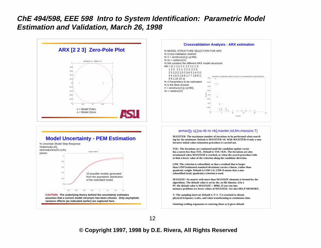
ARX [2 2 3] Zero-Pole Plot

-1

-0.8

-0.6

-0.4

-0.2

0

0.2

0.4

0.6

0.8

1

-1 -0.5 0 0.5 1

OUTPUT # 1 INPUT # 1

x = Model Poleso = Model Zeros

% MODEL STRUCTURE SELECTION FOR ARX% Cross-Validation method% V = arxstruc(z2,[y u],NN);% nn = selstruc(V); % NN contains the different ARX model structuresNN = [1 1 1;1 2 1; 2 2 1;1 1 2; 1 2 2; 2 2 1; 2 2 2; 2 2 3; 2 3 1;3 2 2;3 2 3;4 3 1;4 3 2; 4 4 1;5 5 1;6 6 1;7 7 1;8 8 1; 9 9 1;10 10 1];% 4 Parameters to be estimated % is the Best AnswerV = arxstruc(z2,[y u],NN);nn = selstruc(V)

0

0.005

0.01

0.015

0.02

0.025

0.03

0.035

0.04

0 5 10 15 20 25

# of par`s

loss

fcn

RETURN TO COMMAND SCREEN TO SELECT # OF PARAMETERS TO BE ESTIMATED

Crossvalidation Analysis - ARX estimation

Model Uncertainty - PEM Estimation% Uncertain Model Step Response%idsimsd(u,th);idsimsd(ones(20,1),th);pause;

0

0.2

0.4

0.6

0.8

1

0.2 0.4 0.6 0.8 1 1.2 1.4 1.6

Output number 1

CAUTION: The underlying theory behind the uncertainty estimates assumes that a correct model structure has been chosen. Only asymptotic variance effects (as indicated earlier) are captured here.

10 possible models generatedfrom the asymptotic distributionof the estimated model.

MAXITER: The maximum number of iterations to be performed when search ing for the minimum. Default is MAXITER=10. With MAXITER=0 only a non- iterative initial value estimation procedure is carried out. TOL: The iterations are continued until the candidate update vector has a norm less than TOL. Default is TOL=0.01. The iterations are also terminated when MAXITER is reached, or when the search procedure fails to find a lower value of the criterion along the candidate direction. LIM: The criterion is robustified, so that a residual that is larger than LIM*(estimated standard deviation) carries a linear, rather than quadratic weight. Default is LIM=1.6. LIM=0 means that a non- robustified (truly quadratic) criterion is used. MAXSIZE: No matrix with more than MAXSIZE elements is formed by the algorithms. The default value is set by the .m-file idmsize. (On a PC the default value is MAXSIZE = 4096). If you run into memory problems try lower values of MAXSIZE. See also HELP MEMORY.

T: The sampling interval. Default is T=1. T is essential to obtain physical frequency scales, and when transforming to continuous time. Omitting trailing arguments or entering them as [] gives default

armax([y u],[na nb nc nk],maxiter,tol,lim,maxsize,T)



13

Intermediate Results from Nonlinear PEM Estimation

ITERATION # 3Current loss: 0.001283 Previous loss: 0.001283Current th prev. th gn-dir theta =

-1.3002 -1.3006 0.0003 0.4177 0.4180 -0.0003 0.0670 0.0669 0.0000 0.0418 0.0417 0.0001 -0.2901 -0.2915 0.0014

Norm of gn-vector: 0.001482 <- Norm of gradient vector at zero means that local optimum has been obtained

a1 ->a2 ->b1 ->b2 ->c1 ->

This information appears on OE, BJ, ARMAX, and PEM commands.

Prediction-Error Analysis ARMAX [2 2 1 3]

-0.5

0

0.5

1

0 5 10 15 20 25 30


lag

-0.2

0

0.2

-30 -20 -10 0 10 20 30


lag

All autocorrelation in the residuals has been removed thanks to the C(z) term in the ARMAX model.

% Try ARMAX model instead% th1 = armax(z2,[na nb nc nk]);th1 = armax(z2,[2 2 1 3]);th1 = sett(th1,0.08); % Set the correct sampling interval.

Prediction-Error AnalysisOutput Error [2 2 3]

-0.5

0

0.5

1

0 5 10 15 20 25 30


lag

-0.5

0

0.5

-30 -20 -10 0 10 20 30


lagAutocorrelation in the residuals is unavoidable because of the "lack" of a noise model.

% Go for Output Error% th2 = oe(z2,[nb nf nk])th2 = oe(z2,[2 2 3]);th2 = sett(th2,0.08); % Set the correct sampling interval.

Box-Jenkins [2 1 2 2 3]

-0.5

0

0.5

1

0 5 10 15 20 25 30


lag

-0.2

-0.1

0

0.1

0.2

-30 -20 -10 0 10 20 30


lag

%Box-Jenkins (BJ);% th3 = bj(z2,[nb nc nd nf nk])th3 = bj(z2,[2 1 2 2 3]);th3 = sett(th3,0.08); % Set the correct sampling interval.



14

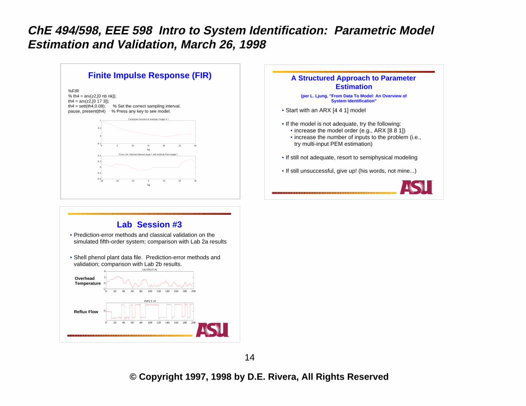
Finite Impulse Response (FIR)

%FIR% th4 = arx(z2,[0 nb nk]);th4 = arx(z2,[0 17 3]);th4 = sett(th4,0.08); % Set the correct sampling interval.pause, present(th4) % Press any key to see model.

-0.5

0

0.5

1

0 5 10 15 20 25 30


lag

-0.4

-0.2

0

0.2

0.4

-30 -20 -10 0 10 20 30


lag

A Structured Approach to Parameter Estimation

(per L. Ljung, "From Data To Model: An Overview of System Identification"

• Start with an ARX [4 4 1] model

• If the model is not adequate, try the following:• increase the model order (e.g., ARX [8 8 1])• increase the number of inputs to the problem (i.e.,

try multi-input PEM estimation)

• If still not adequate, resort to semiphysical modeling

• If still unsuccessful, give up! (his words, not mine...)

Lab Session #3• Prediction-error methods and classical validation on the

simulated fifth-order system; comparison with Lab 2a results

• Shell phenol plant data file. Prediction-error methods and validation; comparison with Lab 2b results.

-2

0

2

4

0 20 40 60 80 100 120 140 160 180 200

OUTPUT #1

0

0 20 40 60 80 100 120 140 160 180 200

INPUT #1

OverheadTemperature

Reflux Flow

che 494/598, eee 598 intro to system identification ... · estimation and validation, march 26,...

Documents