CHASSIS DYNAMOMETER TORQUE

CONTROL SYSTEM DESIGN BY DIRECT

INVERSE COMPENSATION

C.Matthews, P.Dickinson, A.T.Shenton

Department of Engineering, The University of Liverpool,Liverpool L69 3GH, UK

Abstract:This paper presents a methodology for the design of a robust torque control systemfor a transient 1.2m (48in) dia, 120 kW, DC Chassis Dynamometer. The methodincludes system identification of the nonlinear dynamometer torque supply system,linearisation by direct inverse compensation, and linear identification of boththe compensated and uncompensated plants. A combined feedforward-feedbackcontrol structure is proposed and robust feedback controllers are designed using afixed-order parameter space method.

Keywords: Chassis Dynamometer, Direct Inverse Control, Feedback,Feedforward, Identification, Parameter Space, Multiplicative Uncertainty,Nonlinear, Road-Load Simulation.

1. INTRODUCTION

This paper presents a methodology for the designof a combined feedforward-feedback torque con-troller (Figure 1) to be implemented in a chassisdynamometer road-load simulation system. Themethod proposed makes use of direct inverse con-trol similar to that presented in (Petridis andShenton, 2002). The introduction of a direct non-linear inverse compensator provides the combinedadvantage of linearising the systems’ nonlinearbehaviour, and providing a unity path. The tech-nique is evaluated by application to the 1.2mdia , 120 kW, DC chassis dynamometer systemof the Powertrain Control Group, University ofLiverpool.

The nonlinear compensated system is identifiedto generate a number of LTI models, gathered un-der different operating conditions. For comparisonhere a set of LTI models are also identified forthe system without the compensator in place. Foreach set of models, circular uncertainty templates

are defined over the important range of frequen-cies, to model both system nonlinearity and in-trinsic uncertainty. The multiplicative uncertaintyin both compensated and uncompensated plantscan thus be obtained and used to evaluate therobustness of the compensator and to determinethe frequency domain controller specifications.

The identified LTI models are used for the purposeof robust feedback controller design. Solutions arepresented using a parameter space design method(Besson and Shenton, 1997) which derives a loworder controller element for compact implemen-tation. The performance of the controllers is as-sessed through simulation.

2. NONLINEAR INVERSE COMPENSATOR

In the proposed scheme the nonlinear compen-sator is an inverse system model which is identifiedusing inverted input-output data, that is, datawith the input and output causality switched. The

+

-

F

K G+

+

Λ

feedback controller inverse compensator plant

control

effortdesired

torque

sensor noise

feedforward gain

+

+

system

outputerror

Fig. 1. The proposed closed-loop system with feedforward action

system input is varied through its full range of ±10volts while the dynamometer torque response isrecorded.

In the initial implementation of the Liverpool dy-namometer, tested here, it was found that a non-linear non-dynamic gain element provided resultsas good as a dynamic compensator in this casesince the performance of an identified dynamicinverse model was compromised by the oscillatorynature of the load-cell signal.

The system is accordingly modelled as a polyno-mial which is fitted using a least squares algorithmand for which an appropriate model was found tobe 7th order. The resulting function is shown inFigure 2.

−1000 −500 0 500 1000 1500−10

−8

−6

−4

−2

0

2

4

6

8

10

output − torque/Nm

inp

ut

− d

em

an

d/v

olt

s

output/input

7th degree

Fig. 2. Polynomial fit to inverse input/output data

3. LINEAR SYSTEM IDENTIFICATION

A set of linear models are identified for the com-pensated plant Gc and, for comparison purposes,for the uncompensated plant Gu, with each setof models represented as a collection of frequencyresponse models about a centered nominal model.The purpose of this comparative process is todetermine any beneficial effect of compensatingthe plant in reducing model multiplicative uncer-tainty.

3.1 Uncompensated System

Initially, the uncompensated chassis dynamome-ter system is identified as a black box model.

A random-walk excitation signal is applied at thesystem input, and the unfiltered system torque(Nm) response is recorded, as shown in Figure 3.Both input and output signals are logged at an in-terval of 5ms. System identification is carried outusing multiple sets of input-output data, collectedconcurrently. For each set of data, the system isidentified as an ARX model using the MatlabSystem Identification Toolbox (Ljung, 2005).

0 1 2 3 4 5 6

x 104

−1000

−800

−600

−400

−200

0

200

400

600

800

1000

samples

Tor

que

/ Nm

y − Measured Torqueu − Torque Demand

Fig. 3. An example of input/output data collectedfrom the chassis dynamometer.

In order to identify a set of models which ade-quately represents the range of dynamics seen inthe system, the maximum amplitude of the inputsignal is varied for each set of identification datacollected.

In application to the test dynamometer therandom-walk input signal was varied at a rateof 10Hz. The DC drive was operated in a basictorque control mode, requiring an analogue con-trol input of ±10 volts full-range. The dynamome-ter torque output was measured through the re-action force measured by a load-cell mounted be-tween the dynamometer base and a calibratedtorque arm. The load-cell output signal was sam-pled every 5ms.

It was noted that in addition to sensor noise,some structural dynamics were also detected. Ithas been shown (Suzuki and et al, 1994) thatfor the standard torque measurement arrange-ment as used here, the structural dynamics ofthe load measurement arrangement including thetorque arm itself, can be superimposed on themeasured system response. This gives the torquemeasurement an oscillatory nature which is diffi-cult to filter without introducing unacceptable lagto the system. The removal of these unwanted anduncontrollable measurement disturbances wouldprovide significant improvement to the fidelity oftorque measurement.

A parametric ARX structure was selected for themodels with a discrete transfer function of theform:

y

u= G(z) =

θ1z4

z6 + θ2z5 + θ3z4 + θ4z3.... + θ7

The discrete system models were converted tocontinuous models using a bilinear Tustin approx-imation.

The nominal model Go was fitted through thecentre point of the uncertainty circles. The contin-uous nominal model and its parameters are givenin Eqn.1 and Table 1.

y

u= Go(s) =

φ1s8 + φ2s

7 + φ3s6.... + φ8s + φ9

s8 + φ10s7 + φ11s6.... + φ16s + φ17

(1)

Table 1. Uncompensated System ModelParameters

Parameter Value Parameter Value

φ1 0.1538 φ10 92.73

φ2 123.4 φ11 1.602 × 106

φ3 −2.341 × 104 φ12 4.093 × 10

7

φ4 −3.929 × 107 φ13 1.286 × 10

11

φ5 −4.231 × 109 φ14 1.561 × 10

12

φ6 −3.092 × 1012 φ15 1.774 × 10

13

φ7 6.511 × 1014 φ16 7.456 × 10

13

φ8 5.366 × 1015 φ17 3.049 × 10

14

φ9 4.571 × 1016

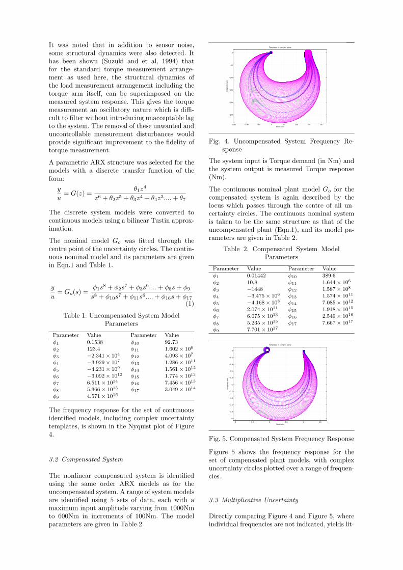
The frequency response for the set of continuousidentified models, including complex uncertaintytemplates, is shown in the Nyquist plot of Figure4.

3.2 Compensated System

The nonlinear compensated system is identifiedusing the same order ARX models as for theuncompensated system. A range of system modelsare identified using 5 sets of data, each with amaximum input amplitude varying from 1000Nmto 600Nm in increments of 100Nm. The modelparameters are given in Table.2.

−150 −100 −50 0 50 100 150 200

−250

−200

−150

−100

−50

0

Templates in complex plane

Real axis

Imag

inar

y ax

is

Fig. 4. Uncompensated System Frequency Re-sponse

The system input is Torque demand (in Nm) andthe system output is measured Torque response(Nm).

The continuous nominal plant model Go for thecompensated system is again described by thelocus which passes through the centre of all un-certainty circles. The continuous nominal systemis taken to be the same structure as that of theuncompensated plant (Eqn.1), and its model pa-rameters are given in Table 2.

Table 2. Compensated System ModelParameters

Parameter Value Parameter Value

φ1 0.01442 φ10 389.6

φ2 10.8 φ11 1.644 × 106

φ3 −1448 φ12 1.587 × 108

φ4 −3.475 × 106 φ13 1.574 × 10

11

φ5 −4.168 × 108 φ14 7.085 × 10

12

φ6 2.074 × 1011 φ15 1.918 × 10

15

φ7 6.075 × 1013 φ16 2.549 × 10

16

φ8 5.235 × 1015 φ17 7.667 × 10

17

φ9 7.701 × 1017

−1 −0.5 0 0.5 1 1.5

−2

−1.8

−1.6

−1.4

−1.2

−1

−0.8

−0.6

−0.4

−0.2

0

Templates in complex plane

Real axis

Imag

inar

y ax

is

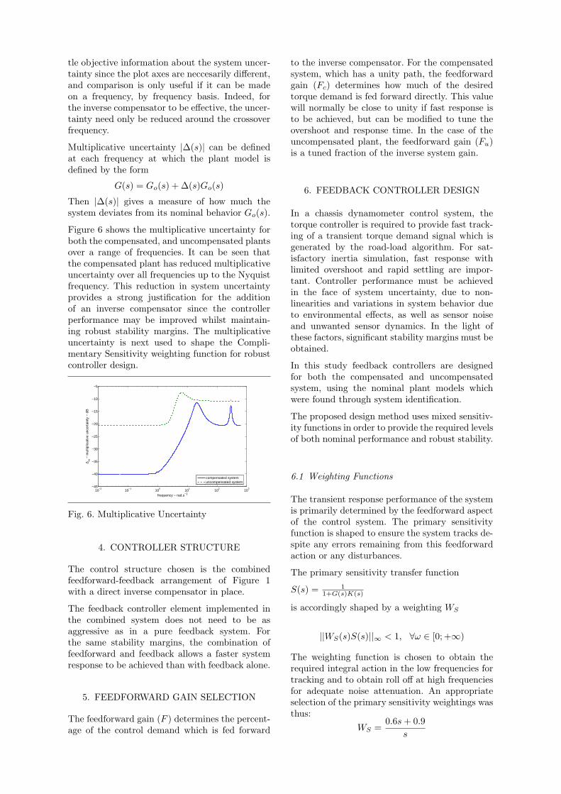
Fig. 5. Compensated System Frequency Response

Figure 5 shows the frequency response for theset of compensated plant models, with complexuncertainty circles plotted over a range of frequen-cies.

3.3 Multiplicative Uncertainty

Directly comparing Figure 4 and Figure 5, whereindividual frequencies are not indicated, yields lit-

tle objective information about the system uncer-tainty since the plot axes are neccesarily different,and comparison is only useful if it can be madeon a frequency, by frequency basis. Indeed, forthe inverse compensator to be effective, the uncer-tainty need only be reduced around the crossoverfrequency.

Multiplicative uncertainty |∆(s)| can be definedat each frequency at which the plant model isdefined by the form

G(s) = Go(s) + ∆(s)Go(s)

Then |∆(s)| gives a measure of how much thesystem deviates from its nominal behavior Go(s).

Figure 6 shows the multiplicative uncertainty forboth the compensated, and uncompensated plantsover a range of frequencies. It can be seen thatthe compensated plant has reduced multiplicativeuncertainty over all frequencies up to the Nyquistfrequency. This reduction in system uncertaintyprovides a strong justification for the additionof an inverse compensator since the controllerperformance may be improved whilst maintain-ing robust stability margins. The multiplicativeuncertainty is next used to shape the Compli-mentary Sensitivity weighting function for robustcontroller design.

10−2

10−1

100

101

102

103

−45

−40

−35

−30

−25

−20

−15

−10

−5

frequency − rad.s−1

∆ m −

mul

tiplic

ativ

e un

cert

aint

y −

dB

compensated systemuncompensated system

Fig. 6. Multiplicative Uncertainty

4. CONTROLLER STRUCTURE

The control structure chosen is the combinedfeedforward-feedback arrangement of Figure 1with a direct inverse compensator in place.

The feedback controller element implemented inthe combined system does not need to be asaggressive as in a pure feedback system. Forthe same stability margins, the combination offeedforward and feedback allows a faster systemresponse to be achieved than with feedback alone.

5. FEEDFORWARD GAIN SELECTION

The feedforward gain (F ) determines the percent-age of the control demand which is fed forward

to the inverse compensator. For the compensatedsystem, which has a unity path, the feedforwardgain (Fc) determines how much of the desiredtorque demand is fed forward directly. This valuewill normally be close to unity if fast response isto be achieved, but can be modified to tune theovershoot and response time. In the case of theuncompensated plant, the feedforward gain (Fu)is a tuned fraction of the inverse system gain.

6. FEEDBACK CONTROLLER DESIGN

In a chassis dynamometer control system, thetorque controller is required to provide fast track-ing of a transient torque demand signal which isgenerated by the road-load algorithm. For sat-isfactory inertia simulation, fast response withlimited overshoot and rapid settling are impor-tant. Controller performance must be achievedin the face of system uncertainty, due to non-linearities and variations in system behavior dueto environmental effects, as well as sensor noiseand unwanted sensor dynamics. In the light ofthese factors, significant stability margins must beobtained.

In this study feedback controllers are designedfor both the compensated and uncompensatedsystem, using the nominal plant models whichwere found through system identification.

The proposed design method uses mixed sensitiv-ity functions in order to provide the required levelsof both nominal performance and robust stability.

6.1 Weighting Functions

The transient response performance of the systemis primarily determined by the feedforward aspectof the control system. The primary sensitivityfunction is shaped to ensure the system tracks de-spite any errors remaining from this feedforwardaction or any disturbances.

The primary sensitivity transfer function

S(s) = 11+G(s)K(s)

is accordingly shaped by a weighting WS

||WS(s)S(s)||∞ < 1, ∀ω ∈ [0;+∞)

The weighting function is chosen to obtain therequired integral action in the low frequencies fortracking and to obtain roll off at high frequenciesfor adequate noise attenuation. An appropriateselection of the primary sensitivity weightings wasthus:

WS =0.6s + 0.9

s

for the compensated plant and

WS =0.3s + 3

s

for the uncompensated plant.

The complementary sensitivity function is alsoused to obtain an additional level of robustness toplant uncertainty. The complementary sensitivitytransfer function

T (s) =G(s)K(s)

1 + G(s)K(s)

is accordingly shaped by a weighting function WT

such that

||WT (s)T (s)||∞ < 1, ∀ω ∈ [0;+∞)

General guidelines (Skogestad and Postlethwaite,1996) are used together with the multiplicativeuncertainty identified to obtain appropriate com-plementary sensitivity weighting functions for thecompensated and uncompensated systems. Forthe test dynamometer these were chosen respec-tively as:

WT =0.5s + 1

1for the compensated plant and

WT =0.5s + 1

10

for the uncompensated plant.

6.2 Parameter Space Design

The feedback controllers for both nonlinear com-pensated and uncompensated systems is designedwith the fixed structure:

K(s) =b2s

2 + b1s + b0

a2s2 + a1s + a0

The feedback controller is designed using the nom-inal plant models and weighting functions WS

and WT selected in each case. The design methodadopted is detailed in (Besson and Shenton, 1997)and has the advantages of being an interactivemethod which allows the time response of thecontrolled system to be tuned, while simultane-ously meeting robust stability margins. Tuningthe controller in this manner has the advantagethat the important effect of the feedforward inthe overall control system can be taken into ac-count directly. It is desirable in this situation,where model uncertainty is great, to use as littlefeedback control action as is possible while stillmeeting the time response specifications.

The following controllers were respectively se-lected for the compensated and uncompensatedsystems:

Kc(s) =0.0014ss − 0.0135s + 0.9983

0.07s2 + s

Ku(s) =0.0009s2 + 0.0048s + 0.0267

0.07s2 + s

The time response performance of the closed loopsystems was checked through simulation. Feed-forward gains (Fc and Fu) were tuned to eitherreduce overshoot or to reduce response time de-pending upon the basic performance of the feed-back controller and initial feedforward gain se-lected (Fc = 0.99 and Fu = 0.0050). Figure 7shows the simulated closed-loop system responsefor both systems. It can be seen that the compen-sated system has a significantly faster responsetime (82.5ms), and settling time (565ms) than theuncompensated system (214ms and 1.15s respec-tively), while the compensated system displaysalmost the same overshoot (37 percent comparedwith 33 percent) during initial response.

0 0.2 0.4 0.6 0.8 1 1.2 1.4 1.6 1.8 2−200

0

200

400

600

800

1000

1200

Time / seconds

Tor

que

/ Nm

compensated system responseuncompensated system response90% response102% response98% response

Fig. 7. Controlled system response

In order to conservatively establish system ro-bustness of the controller on the nonlinear plant,robustness to possible rapid switching between thecomponent LTI models can be established by acritical disk (Petridis and Shenton, 2002) analy-sis. This provides an additional level of conser-vative robustness over that required for a purelylinear uncertain system by representing a regionaround the -1 point in the Nyquist plot of theloop functions Lc = KcΛGc and Lu = KuGu.The circular disks represent a conservative regionoutside which which system stability can be guar-anteed. The disks are each defined by two points,

α =|G|

min

|G|nom

and β =|G|

max

|G|nom

which are centred on

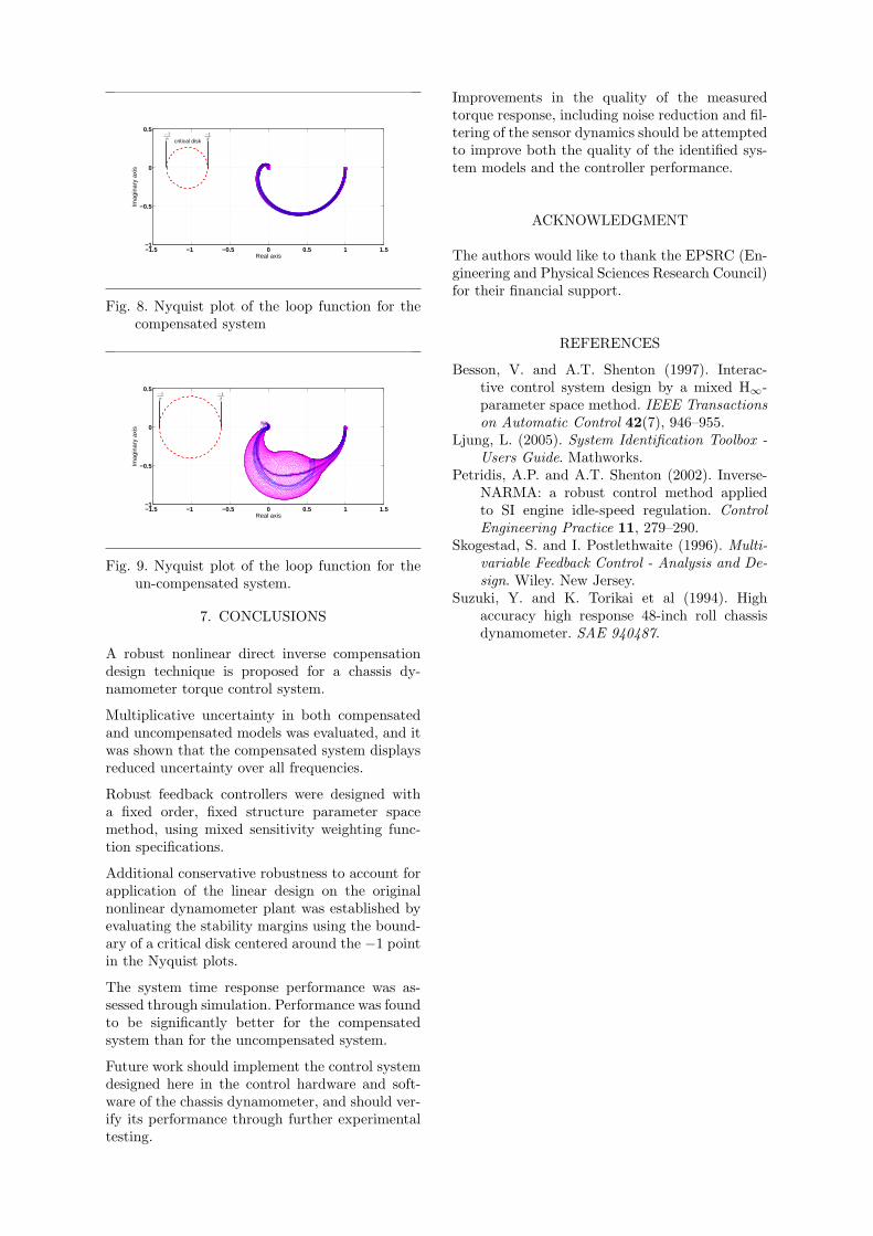
the real axis. Figures 8 and 9 show the Nyquistplot (including uncertainty disks), with a criticaldisk plotted around the -1 point.

Comparison of Figure 8 and Figure 9 shows thatthe compensated plant, with its superior timeresponse performance, also guarantees a superiorstability margin.

−1.5 −1 −0.5 0 0.5 1 1.5−1

−0.5

0

0.5

Real axis

Imag

inar

y ax

is−1α

−1βcritical disk

Fig. 8. Nyquist plot of the loop function for thecompensated system

−1.5 −1 −0.5 0 0.5 1 1.5−1

−0.5

0

0.5

Real axis

Imag

inar

y ax

is

−1β

−1α

Fig. 9. Nyquist plot of the loop function for theun-compensated system.

7. CONCLUSIONS

A robust nonlinear direct inverse compensationdesign technique is proposed for a chassis dy-namometer torque control system.

Multiplicative uncertainty in both compensatedand uncompensated models was evaluated, and itwas shown that the compensated system displaysreduced uncertainty over all frequencies.

Robust feedback controllers were designed witha fixed order, fixed structure parameter spacemethod, using mixed sensitivity weighting func-tion specifications.

Additional conservative robustness to account forapplication of the linear design on the originalnonlinear dynamometer plant was established byevaluating the stability margins using the bound-ary of a critical disk centered around the −1 pointin the Nyquist plots.

The system time response performance was as-sessed through simulation. Performance was foundto be significantly better for the compensatedsystem than for the uncompensated system.

Future work should implement the control systemdesigned here in the control hardware and soft-ware of the chassis dynamometer, and should ver-ify its performance through further experimentaltesting.

Improvements in the quality of the measuredtorque response, including noise reduction and fil-tering of the sensor dynamics should be attemptedto improve both the quality of the identified sys-tem models and the controller performance.

ACKNOWLEDGMENT

The authors would like to thank the EPSRC (En-gineering and Physical Sciences Research Council)for their financial support.

REFERENCES

Besson, V. and A.T. Shenton (1997). Interac-tive control system design by a mixed H∞-parameter space method. IEEE Transactionson Automatic Control 42(7), 946–955.

Ljung, L. (2005). System Identification Toolbox -Users Guide. Mathworks.

Petridis, A.P. and A.T. Shenton (2002). Inverse-NARMA: a robust control method appliedto SI engine idle-speed regulation. ControlEngineering Practice 11, 279–290.

Skogestad, S. and I. Postlethwaite (1996). Multi-variable Feedback Control - Analysis and De-sign. Wiley. New Jersey.

Suzuki, Y. and K. Torikai et al (1994). Highaccuracy high response 48-inch roll chassisdynamometer. SAE 940487.