Charging-as-a-Service: On-demand battery delivery for light-duty electricvehicles for mobility service

Shuocheng Guoa, Xinwu Qiana,∗, Jun Liua

aDepartment of Civil, Construction and Environmental Engineering, The University of Alabama, Tuscaloosa, AL35487, United States

Abstract

This study presents an innovative solution for powering electric vehicles, named Charging-as-a-Service (CaaS), that concerns the potential large-scale adoption of light-duty electric vehicles(LDEV) in the Mobility-as-a-Service (MaaS) industry. Analogous to the MaaS, the core idea ofthe CaaS is to dispatch service vehicles (SVs) that carry modular battery units (MBUs) to provideLDEVs for mobility service with on-demand battery delivery. The CaaS system is expected totackle major bottlenecks of a large-scale LDEV adoption in the MaaS industry due to the lack ofcharging infrastructure and excess waiting and charging time. A hybrid agent-based simulationmodel (HABM) is developed to model the dynamics of the CaaS system with SV agents, and atrip-based stationary charging probability distribution is introduced to simulate the generation ofcharging demand for LDEVs. Two dispatching algorithms are further developed to support theoptimal operation of the CaaS. The model is validated by assuming electrifying all 13,000 yellowtaxis in New York City (NYC) that follow the same daily trip patterns. Multiple scenarios areanalyzed under various SV fleet sizes and dispatching strategies. The results suggest that anoptimal CaaS system with 250 SVs may serve the LDEV fleet in NYC with an average waitingtime of 5 minutes, save the travel distance to visit charging station at over 50 miles per minute,and gain considerable profits of up to $50 per minute. This study offers significant insights intothe feasibility, service efficiency, and financial sustainability for deploying city-wide CaaS systemsto power the electric MaaS industry.

Keywords: Charging-as-a-Service, Mobility-as-a-Service, Electric Vehicles, System Simulation

1. Introduction

The transportation sector has witnessed two major revolutions in the past decade that havebeen reshaping the mobility landscape of urban travelers: one being the rapid growing adoptionof electric vehicles (EVs) in replace of the traditional gasoline vehicles advances, while the otherattributing to the unprecedented rise of the Mobility-as-a-Services (MaaS). In particular, over 2.1million EVs were sold in 2019 globally, marking a 40% annual growth rate since 2010 [1]. Meanwhile,the MaaS market has seen tremendous growth since 2014, with the number of ride-hailing tripsincreased from 60,000 to over 750,000 in New York City (NYC) alone. Given the vast numberof daily trips from the MaaS market, the use of EVs signifies opportunities to alleviate the worseemission and energy consumption situations in large cities [2]. Nevertheless, the two streams of

∗Corresponding author.Email addresses: sguo18@ua.edu (Shuocheng Guo), xinwu.qian@ua.edu (Xinwu Qian), jliu@eng.ua.edu (Jun

Liu)

Preprint submitted to Elsevier November 24, 2020

arX

iv:2

011.

1066

5v1

[m

ath.

OC

] 2

0 N

ov 2

020

revolution barely converge. Despite the ambitious plan from the major transportation networkcompanies (TNCs) for electrifying their fleet [3], less than 0.2% of the fleet for Uber and Lyft areEVs.

There are at least three critical barriers that prevent the widespread commercial adoption oflight-duty electric vehicles (LDEVs) in the MaaS industry. The first barrier attributes to the lack ofsufficient charging facilities in urban areas. For instance, there were 450 public charging stations inNYC providing 931 Level 2 chargers and 82 DC Fast chargers as of 2019 [4], which can hardly satisfythe enormous charging needs if we fully electrify the fleet of major MaaS operators with over 100,000vehicles. Tesla has recently announced the Supercharger fair use policy [5], banning commercialEVs from using its Supercharger stations. The second barrier arises from insufficient land spaceand power grid supply to allow for the massive construction of charging facilities in MaaS’s coreservice areas. This indicates that the charging facilities have to be located at distant locations,which leads to the third barrier due to excessive travel time to-and-from a charging station, longcharging time, and prolonged waiting time at the station during peak hours. During peak hours inShenzhen, China, electric taxi drivers have to wait at least 30 minutes for an available charger[6].These barriers pose emerging needs for a dedicated charging solution that tailors to MaaS in orderto promote the electrification of the MaaS industry.

Existing studies of charging facility planning primarily focused on locating fixed charging sta-tions (FCS), battery swapping stations (BSS), and more recently, the deployment of mobile chargingsystems (MCS). Early work proposed the optimal design of FCS locations under the network equi-librium of the coupled road and power networks [7], recharging time and flow-dependent energy [8],and the multi-class user equilibrium [9]. Moreover, the concept of charging lanes envisions wirelesscharging and motivates studies on the deployment of the charging lanes [10, 11] and its co-planningproblem with existing FCSs [12]. More recently, researchers investigated the optimal design ofboth location and capacity for FCSs under the consideration of long-distance travel [13], electricbus charging stations [14, 15], the waiting and charging spots for electric taxis [16], and road userswith travel and charging equilibrium [17].

For the deployment of BSSs, the objectives of the early work included developing a cost-effectivesubscription based swapping service [18], maximizing the net present value or profit [19, 20], min-imizing the long-term operating costs [21], and reducing queuing time under a city-wide electrictaxi fleet [22]. While there exist plentiful studies on FCS and BSS, the research on mobile chargingfacilities is still in the early stage. The early study considered a mobile charging platform con-sisting of portable plug-in chargers and mobile swapping stations [23]. With the incorporation offast charging technology, more recent studies explored the operation of commercial mobile chargingfacilities including mobile charging stations [24] and mobile swapping vans [25].

Although the aforementioned studies on charging facility preparation can promote the adoptionof privately owned EVs, they may hardly benefit LDEVs for the MaaS industry considering thedistinct operation dynamics. We briefly summarize the features of the charging facilities, includingtheir barriers to promote the MaaS industry in Table 1. As discussed previously, these key barriersconsist of the high implementation cost, limited space available for charging facilities, the inter-ruption of mobility services for charging batteries, and the difficulties in coordinating the chargingneeds among large-scale LDEVs. We note that the mobile modular units, such as prototypes ofSparkCharge [26], promises a more flexible and portable scheme. The mobile unit consists of onemodular charger unit and up to five modular battery units (MBUs). The MBU can stack on topof one another and work together, with each MBU offers at least 12 miles of range under thecharging speed of at least one mile per minute [26], which is sufficient to satisfy the service needsof LDEVs in urban areas and makes “charge-as-you-go” possible. And the above barriers can belargely resolved if there exists a system that can optimally coordinate the delivery of the MBUs

2

with the charging needs from the LDEVs. Aside from the daily use scenarios, we remark that theCaaS using the MBUs will also be more resilient to extreme scenarios (e.g., charging demand surgein peak hours, power outage, severe weather), outperforming the mobile charging station due to itsportability and flexibility. With a sufficiently large SV fleet and additional MBUs as the back-up,the CaaS can ensure the functionality of the LDEV fleet under those extreme cases to maintain ahigh service level and constant power supply. These features motivate us to explore the innovativecharging solution for powering LDEV fleet and investigate the feasibility and performances of thecity-wide adoption of such charging systems.

Table 1: Summary of charging facilities and infrastructure

Facilitytype

Chargingspeed(mile/min)

Location Configuration (perunit)

Barriers for the MaaS Source

Fixedcharger

0.03 - 4 Fixed Installationcosts:$4,000-$51,000(DC fast)

High cost, space limita-tion, long charging time,service interruption forcharging, difficult to coop-erate large-scale chargingevents

[27] [28]

Batteryswappingstation

Swap in2.5 min

Fixed Construction cost:$800,000; main-tenance costs:$30,000/year

High cost, space limita-tion, service interruptionfor charging, restriction onthe type of battery used

[22] [29]

Mobilechargingstation

Up to 0.5 Flexible Weight: 1860 lbs;battery capacity:80 kWh

Not portable, capacityand weight limitation fordelivery

[30]

Mobilemodularunits

1 Flexible Weight: 19.8 lbs(MCU), 48.4 lbs(MBU); battery ca-pacity: 3.5 kWh

Small capacity, requiresthe support of optimal de-livery algorithms

[26]

In this study, we make the initial attempt to investigate an emerging charging solution forelectrifying the MaaS industry, named Charging-as-a-Service (CaaS). Unlike the current notion ofCaaS, which mainly offers subscription service for fixed chargers [31] [32], the CaaS discussed in thisstudy is a more typical on-demand charging service via MBU delivery which is motivated by therecent advances in the modular fast-charging technology [26, 33]. We consider a centralized CaaSsystem that dispatches service vehicles (SVs) to the LDEV’s requested charging location to replacethe depleted MBUs with fully-charged ones. A hybrid agent-based model(HABM) is developed tosimulate the joint operation of LDEVs and the SV fleet in a CaaS system, aiming at providingLDEVs an efficient charging service while evaluating the operation performances, benefits, andfinancial sustainability of developed CaaS systems. The main contributions of our work can besummarized as follows:

1. A CaaS operation framework is designed to provide on-demand battery delivery services tosatisfy the changing needs of city-wide LDEV fleet for mobility service.

2. A hybrid agent-based model is developed which consists of stationary charging demand gen-eration for large-scale LDEV fleet and agent-level service dynamics for the SV fleet.

3. Dispatching algorithms are developed to support the optimal operation of SVs that minimizethe average waiting time for the charging requests.

3

4. Real-world numerical experiments are conducted to examine the applicability of the CaaSsystem, which examines the service dynamics and quantifies the savings of out-of-service timeand charging miles and its financial sustainability when compared to charging at the FCSs.

The rest of the paper is organized as follows. The next section introduces the business model ofCaaS, the HABM framework, and the performance metrics. In Section 3, we present the numericalexperiments for electrifying the NYC taxi market as a case study and discuss the results andinsights. Finally, section 4 concludes our work with key findings, recommendations of CaaS systemconfigurations, and future directions.

2. Model

2.1. Preliminaries

This study models the dynamics of the CaaS system at the zonal level with discrete time steps.In the CaaS system, there are two types of interacting dynamics: (1) the movement of LDEVs, bothserving passenger trips as well as relocations, that results in charging requests (demand) and (2) themovement of SVs that provide the MBU delivery services to the site of service requests (supply).The LDEVs will make reservations for the MBU replacement before running out of electricity andmeet SVs at the scheduled location and time. The out-of-electricity LDEVs will resume their tripservice upon the delivery of the MBUs, with MBUs function as power banks that provide sufficientpower to sustain travels in urban areas (1 mile per minute). The SVs will keep serving chargingrequests from LDEVs until consuming all fully-charged MBUs, and the SVs will then return tothe depot to unload empty MBUs and reload with fully charged ones. The interactions betweenthe LDEV and SV fleet are ruled by the dispatching policies that assign the available SVs to therequested LDEVs to minimize the LDEV fleet’s total waiting time.

We start with three basic scenarios that illustrate the operation of the CaaS system, as shownin Figure 1. Scenario 1 shows how the CaaS system processes reservation requests for chargingservice. The blue LDEV from the origin (O1) sends out a request with its destination (D1) andestimated arrival time to D1. The system then matches this request with the orange SV at O1

′, and

the LDEV and SV will meet at the D1. Scenario 2 represents an LDEV being served, in which boththe green LDEV and the assigned green SV have reached the destination (D2), and the SV driveris replacing the depleted MBUs with fully-charged ones. Scenario 3 describes that the red SV hastwo scheduled red LDEVs with requested destinations at D3-1 and D3-2. When the SV is en route,one LDEV is waiting for SV at D3-1 and the other is on its way to D3-2. When the SV is out ofMBUs after serving the request at D3-2, it will move back to the depot at D3-3 to replenishmentfully-charged MBUs. The following sections will introduce the details on the generation of chargingdemand, the operation of the CaaS in the hybrid agent-based model, and three different dispatchingpolicies.

4

Figure 1: An illustration of the CaaS system with three basic scenarios consisting of LDEV, SV, and the depot. Thisillustration chart is modified from an open-source template in the Icograms [34].

2.2. Generation of stationary charging demand

One bottleneck for planning charging infrastructure for the LDEVs is the ability to characterizethe distribution of charging needs. Unlike private EVs where charging locations can be easilyestimated, the location of charging needs of LDEVs depending on the stochastic trip and relocationactivities. To address this issue, we introduce a stochastic model which considers moving activitiesin the MaaS system as a discrete-time Markov chain, following the preliminary analyses from theauthors’ prior work [35]. With the zonal representation, the Markov chain regards each zone as astate and the movement between zone i and zone j as the transition probability Pij . In this regard,the MaaS system dynamics are modeled as an event-based system with each event being eitherserving a trip or performing a relocation. The sequences of moving events will drive the LDEVsbetween zones and eventually incur charging requests.

Specifically, we consider a centralized MaaS service system where the LDEVs follow trip andrelocation sequences designated by the platform. We divide the operation hours into discrete timeintervals, where the passenger demand pattern is assumed to be stable within each time interval.While a specific trip sequence may differ for individual LDEVs, their collective movement patternsat time t can be measured statistically. That is, the probability πti(k) that an arbitrary LDEV willremain at zone i following kth event can be described as:

πti(k) =

N∑j=1

πtj(k − 1)P tji (1)

With a sufficient large number of events (trips), we will have the stationary probability that anarbitrary LDEV will be in a specific zone following any event as:

πt = πtP t (2)

Moreover, for each time interval t, the battery of an LDEV at the end of each movement eventmay fall into one of the two categories: (1) sufficient battery and continue to the next movementor (2) recharge the battery by the CaaS and then continue to the next movement. Denote Eij asthe expected electricity consumption between zone i and zone j, we can therefore represent the

5

expected battery consumption for any LDEV that arrives in zone i as:

eti =

∑Nj=1 π

tjP

tjiE

tji∑N

j=1 πtjP

tji

(3)

We note that both P tij and Et

ij can be obtained by mining the historical daily operation data fromthe large-scale LDEV fleet. Let CLDEV be the battery capacity and δ be the charging threshold(e.g., an LDEV will not charge until the battery level is below δCLDEV , the probability that anarbitrary LDEV that arrives in zone i and has its battery below the threshold (therefore needsrecharge) follows:

P t(Xchargei = 1) =

πti eti

CLDEV (1− δ)(4)

where a detailed derivation can be found in [35]. Let K be the average number of trips that anLDEV may complete per unit time, NLDEV be the LDEV fleet size and Nw be the number ofLDEVs that are awaiting recharging of the battery, we can eventually express the arrival rate ofcharging demand per unit time in a given zone i as:

λti = Kπti(NLDEV −Nw)P t(Xchargei = 1) (5)

where we have NLDEV −Nw be the set of active LDEVs that will generate charging requests, andKπti represents the expected number of trips that may arrive in zone i per unit time per LDEV. Wecan then use the Poisson arrival process to generate the arrival charging demand following equa-tion 5. This helps avoid the expensive simulation of the actual moving trajectories for individualLDEVs by directly sampling the charging demand at the zonal level, which is much more scalableand contributes to significant speedups of the simulation when the fleet size is large.

2.3. The hybrid agent-based model

Given the arrival of charging demand, the dynamics for the fleet of SVs are simulated followingthe agent-based modeling framework, as shown in Figure 2. The simulation framework takes theSV fleet size (NSV ) and battery capacity of the MBU (CMBU ) as input and follows three differentpolicies to match available SVs to charging requests. And Cb denotes the remaining number offully-charged MBUs on the SV, which is limited by the capacity of the SV (C). The outputs arethe performance metrics of the CaaS system in serving the generated charging requests that areparameterized by E,P ,N ,π, and K.

The framework describes the criterion on how the SV agents are connected to the chargingrequests, as discussed in the preliminary section, and how the SV agents are navigated betweenthe charging depot and charging requests in the HABM. Specifically, we define that each SV agentmay be in one of the following five states:

• Idle (I). An SV is in I state if it has sufficient fully-charged MBUs to serve future chargingrequests and is currently not assigned with a delivery task.

• Relocating (R). Once an SV is matched with a charging request, it will remain in R stateuntil it arrives at the requested service location.

• Ready for service (S). An SV is in S state if it arrives at the requested service location,and the SV will then replace the depleted MBU with a fully-charged one.

6

Start tick 𝑡𝑡

𝑁𝑁𝑆𝑆𝑆𝑆 ,𝐶𝐶𝑀𝑀𝑀𝑀𝑀𝑀 ,𝐶𝐶𝑏𝑏 ,𝐶𝐶

Status == I?

𝐶𝐶𝑏𝑏 > 0?

𝑡𝑡𝑎𝑎 − 𝑡𝑡 < 0?

Serve

Status: =I

𝐶𝐶𝑏𝑏 = 𝐶𝐶?

Status: =I

𝑡𝑡𝑑𝑑 = 𝜙𝜙?

Status: =M

Arrival time to depot: 𝑡𝑡𝑑𝑑

𝑡𝑡𝑑𝑑 − 𝑡𝑡 < 0 ?

Status: =D(reload MBU)

Status == D?

N

Y

N

Y

Y

Y

Status process for each SV i ∈ 𝑉𝑉

N

Y

N

𝐸𝐸𝑡𝑡 ,𝑃𝑃𝑡𝑡 ,𝑁𝑁𝐿𝐿𝐿𝐿𝐿𝐿𝑆𝑆 ,𝜋𝜋𝑡𝑡 ,𝐾𝐾Update SV status

Demand 𝜆𝜆𝑡𝑡

Matching

Status: =R; arrival time: 𝑡𝑡𝑎𝑎

Y

Y

N

N

𝑡𝑡 > 𝑇𝑇 ?

Y

𝑡𝑡 = 𝑡𝑡 + 1

Update demand

End

N

N

Figure 2: Integrated HABM framework for modeling the CaaS system.

• Moving back to depot (M). When an SV runs out of the fully-charged MBU, it will beassigned in D state and start moving back to the depot location.

• At depot (D). An SV is in D state if it has returned to the depot. The SV will then unloadthe depleted MBUs and reload with fully-charged MBUs.

To develop the HABM framework, we make the following assumptions:

1. We assume that each SV will have sufficient range to deliver all the MBUs without any

7

interruption, and the SV will restore its full range while at the depot.

2. Since a zone-based HABM framework is adopted, the relocating distance between zone i andzonej is sampled from the distribution of observed travel duration (e.g., from historical data)between the two zones, which is assumed to follow a log-normal distribution in our study.

3. The SVs are operated by a central dispatching platform. This means that the SV driversneed to follow assigned service order and will not cruise for orders on their own.

In each simulation tick t, the states of SVs will be based on if there are charging requests in theservice area and if there are available fully-charged MBUs. For regular MBU replacement services,an SV will undergo the I-R-S-I process as the charging requests arrive: from I to R when matchedwith a charging request, from R to S while relocating to the service location, and from S back to Iwhen the service is completed. The I-R-S-I process continues until the SV runs out of fully-chargedMBUs, where the SV will then be redirected to follow the S-M-D-I process to send the depletedMBUs back to the depot and reload with fully-charged MBUs to maximum capacity. The SV willchange from S to M when the service is completed, and all fully-charged MBUs are consumed, fromM to D when the SV is navigated back to the depot for reloading new MBUs, and from D to Iwhen the SV completed the reloading process and is again available for the services.

2.4. Dispatching policy

One key component of the HABM framework, as shown in Figure 2, is the matching module,which sets up the rule on how available SVs will be dispatched to satisfy the charging requests.In this study, we consider three dispatching policies that match available SVs with charging re-quests. The first policy, as a benchmark scenario, is the greedy first-come-first-serve policy (FCFS).The other two policies, namely the optimal matching with local information (OML) and optimalmatching with dynamic detour (OMDD), are developed under the consideration of minimizing totalmatching cost (defined as the waiting time of charging requests). They differ in the set of SVs thatare available for the dispatching policy at each time step. OML can only see SVs that are currentlyin idle state, while OMDD can control the entire SV fleet despite of the SVs’ state. In this regard,OML is more suitable for the CaaS system with independent SV drivers while OMDD is designedfor fully-cooperative fleet.

2.4.1. First-come-first-serve

Under the FCFS policy, LDEVs’ charging requests are served in the order in which they arereceived with the nearest available SV. The charging requests are sorted in the ascending orderin the request list L based on their request time. At each simulation tick, requests are matchedsequentially with available SVs, and travel cost Tij is incurred for a request in zone i that is matchedwith an SV in zone j. We note that Tij is a random variable to reflect the impacts of stochasticlocations of the charging request and the LDEV in their corresponding zones. For each simulationtick, the FCFS terminates when either all charging requests are matched or all available SVs areoccupied. All matched charging requests are then removed from L. Under the FCFS policy, thematching can be solved with time complexity of O(|L|log(|L|)+|L|N), where N denotes the numberof available SVs.

We note that the FCFS policy will likely lead to more vacant trips and result in low SVfleet efficiency with its sequential matching scheme. For instance, when charging requests emergebetween the central area and distant area in turns, the SVs have to travel a long distance back andforth to satisfy all requests. In this case, all LDEVs have to wait long for the SVs, and the lowlevel of service potentially results in a higher unsatisfied rate. Next, we will explore two optimaldispatching policies that improve both LDEV users’ level of service and SV fleet efficiency.

8

2.4.2. Optimal matching with local information

OML policy aims to minimize the total waiting cost of charging requests, including relocationcost and current waiting cost. With local information, the OML policy will only dispatch SVs thatare currently in I state. In each tick t, candidate SVs are assigned following an optimal dispatchingprotocol f(Vt,Dt), where Vt denotes the set of available SVs and Dt for the set of LDEVs thatneed MBU replacements. When LDEV k in zone i schedules a MBU replacement at destination jin time t, the platform will set its future service time as Ti = τ tij + t for the charging request, whereτ tij is the estimated relocation time from zone i to zone j in time t.

To derive an optimal assignment between SVs and LDEVs, we formulate the OML strategy asa minimum weight bipartite matching problem with Vt,Dt as the two sets of nodes for each timestep t. Considering edges connecting each pair of nodes in the two sets, the weight on each edge ismeasured as the difference between ctij + t and Tj , for all i ∈ Vk and j ∈ Dk. With ctij being therelocation time from SV i to request j, the time difference may lead to early arrival of SV if ctij + tis smaller than Tj , or late arrival otherwise. In our study, we penalize both early and late arrivalsbut with a penalty factor 0 ≤ η ≤ 1 to favor early arrival over late arrival. In this regard, the OMLdispatching policy at time t can be mathematically formulated as:

minx

∑i∈Vt

∑j∈Dt

xij(max(0, ctij + t− Tj) + ηmax(0, Tj − ctij − t)

)subject to

∑i∈Vt

xij = 1,∀ i ∈ Vt

∑j∈Dt

xij = 1, ∀ i ∈ Dt

xij ∈ {0, 1}

(6)

The constraints in equation 6 state that each available SV is assigned to only one LDEV, andvice versa. In most cases, the cardinality of Vt and Dt will not be equal so that a perfect matchingcan not be established. To address this issue, we augment the set of smaller cardinality with||V| − |D|| dummy elements, and mark the weight on edges that connect to dummy modes with anarbitrarily large value M . Consequently, one can solve equation 6 with augmented sets to find theoptimal dispatching using the Hungarian method [36], which can solve the problem in O(N3) time(N being the cardinality of the augmented set).

As compared to the FCFS policy, the OML performs matching at the system level, whichdelivers optimal local dispatching of SVs. However, the assignment using local information maynot ensure long-term optimal dispatching, as new requests being generated after the matchingdecision has been made. This motivates the third policy as an optimal matching with a dynamicdetour to tackle this issue.

2.4.3. Optimal matching with dynamic detour

OMDD seeks to mitigate the OML policy’s drawback due to its lack of flexibility for dynamicallyupdating the assignment with the arrival of new charging requests. This is especially the case whenan SV is scheduled to arrive much earlier than the service time, and the lead time is sufficient toallow for additional services.

The OMDD inherits the overall framework of OML, with the major differences being that(1) an SV can have more than one service request scheduled, e.g., the schedule of SV j beingSj = {m1

j ,m2j , ...,m

nj }, and (2) the matching cost is derived by inspecting if a valid gap is available

for additional service in between successive scheduled requests. At time step t, we define that an

9

additional service mxj = (x, Tx) can be inserted in between SV j’s consecutive requests mk

j ,mk+1j ,

if the following conditions are satisfied:

Tk+1 − Tk ≥ τ tkx + τ txk+1 (7)

so that there are sufficient time for the SV j to travel from request k to x and then from x to k+ 1.In addition, the new request can be inserted to the beginning of Sj if

T1 − t ≥ τ tjx + τ tx1 (8)

with τ tjx being the travel time from SV j’s current location to the location of new request x. Finally,the new request can always be appended to the end of Sj (n+1 th position).

Let ckjx be the valid cost for inserting x to the kth request in Sj , we have

ckjx =

η(T1 − t− τ tjx − τ tx1), if k = 1

η(Tk+1 − Tk − τ tkx − τ txk+1), if 1 < k ≤ nmax(0, t+ τ tnx − Tx) + η(max(0, Tx − τ tnx − t)), if k = n+ 1

(9)

And the matching cost for SV j and service request x is determined by the minimum of all validcosts:

c∗jx = minkckjx (10)

With the definition of c∗jx, the dispatching strategy of SVs under the OMDD policy can beagain obtained by solving the minimum weight bipartite matching problem for each time step t.Different from the OML policy, Vt now includes all SVs in the CaaS system, and the problem canbe formulated as:

minxij

∑i∈Vt

∑j∈Dt

xijc∗ji

subject to∑i

xij = 1, ∀ i ∈ Vt∑j

xij = 1, ∀ i ∈ Dt

xij ∈ {0, 1}

(11)

Similar to the OML policy, the optimal solution under the OMDD policy can also be solved by theHungarian method in O(N3) time.

2.5. Performance metrics

The performance of the CaaS system will be evaluated via simulations with the HABM and thethree dispatching policies, with the following major performance metrics.

The first metric calculates the savings in out-of-service duration (min) based on the gap betweenthe average waiting time of CaaS and the time it requires to visit and charge at an FCS:

Ro = TFCS − TCaaS ∗CLDEV

CMBU(12)

where TCaaS is the average waiting time in CaaS and TFCS captures the average time requiredto visit and charge at an FCS. CLDEV is battery capacity for the LDEV and CMBU is battery

10

capacity of MBUs. In Equation 12, we use CLDEVCMBU

to convert the corresponding waiting time forCaaS into the full-charge-equivalent (FCE) waiting time, so that we account for the more numberof MBU replacements to achieve the same battery level as the full charging at an FCS.

Similarly, we can quantify the saving of charging distance by computing the gap in trip milesper unit time between the LDEVs’ expected travel distance to visit the nearest FCS and SVs’operation distances:

Rd =1

∆T

(dFCS ∗Ns − dSV ∗

CLDEV

CMBU

)(13)

where ∆T is the duration of the simulation process, dFCS is the average travel distance (mile) toFCSs, and dSV represents the total miles traveled by the SV fleet.

In addition, it is also important to understand the financial sustainability of the proposedCaaS services. This requires measuring the cost and revenue incurred during daily operations. Weconsider that the total CaaS cost includes the capital cost (e.g., the procurement of SVs, MBUs),labor cost for SV drivers, and the operation cost. Specifically, the labor cost is quantified by servednumber of charging requests and operation cost is associated with the total miles traveled. Weexpress the total CaaS cost as:

QCaaS = NSV (QSV + C ∗QMBU + dSV ∗ q) +QLVs (14)

where QSV , QMBU are the per-unit purchase cost of SV and MBU, respectively. C is the SVcapacity for MBUs, q is the coefficient for operation cost and QL represents the labor cost perserved request.The average operation cost is set as 57.3 cents per mile following the statistics forthe P70D step van used by the UPS [37].

To evaluate the revenue generated by the CaaS, we first calculate the willingness-to-adopt ofCaaS as compared to alternate charging mode based on the average waiting time and the per-service price p. For simplicity, we use the binary logit function to model the charging choices [38]and measure the probability P i

CaaS that LDEV i may adopt the CaaS as follows:

P iCaaS =

1

1 + exp(U iFCS − U i

CaaS

) (15)

U iCaaS = −

(p+ κW i

s

)∗ CLDEV

CMBU−Qc (16)

U iFCS = −κTFCS −Qc (17)

In equation 15, U iCaaS and U i

FCS refer to LDEV i’s perceived utilities for using the CaaS andthe FCS, respectively. κ is the time value for LDEV users, which is considered as $1/min. Qc isthe electricity cost for fully charging the battery on a typical LDEV. Here we consider a 50-kWhbattery capacity for the LDEV and the electricity price of $0.135/kWh, so that Qc takes the valueof 6.75. Similar to the calculation of Ro and Rd, the FCE values are also used here to convert thecost per CaaS service into an equivalent cost for a full charge of the LDEV battery, and W i

s hererepresents the waiting time for LDEV i. The revenue and cost eventually enables us to evaluatethe profit level of the CaaS under different scenarios.

The parameter setting in this study is summarized in Table 2. In particular, CMBU is assumedas 14 kWh according to the SparkCharge configuration [26]. And we assume the SV capacity fora 4-modular MBU count C as 50, by considering the SV’s payload capacity [39], and we ensurethat the total weight of 200 (50 × 4) MBUs is under the payload capacity. In this case, each SV

11

will carry 50 sets of four-module MBU, where each set can provide the LDEVs with 14 kWh ofelectricity or at least 48 miles of drive range.

Table 2: Parameter setting used in this study

Parameter Value Description

QSV $40,000 SV unit priceQMBU $10,000 4-modular MBU unit priceq $0.573 per mile SV operation costC 50 count SV’s capacity for four-module MBUCLDEV 50 kWh LDEV battery capacityCMBU 14 kWh MBU battery capacityκ $1 per min time valueTFCS 90 min average waiting time and driving time to FCSdFCS 15 mile average relocation distance to FCS

3. Results

3.1. Data

We choose New York City (NYC) as the study area for our numerical experiments. We leverageNYC taxi trip data in 2013 [40] to obtain occupied and vacant trip sequences, where these tripsare preprocessed and aggregated into 263 taxi zones that cover Manhattan, Brooklyn, Queens,Bronx, Staten Island, and Newark Liberty International Airport (EWR). The 2013 taxi trip datais used instead of more recent data as it represents the most recent taxi dataset in NYC that hasthe encrypted medallion ID available, based on which we can track complete trip sequences ofindividual taxis. This data allows us to calibrate πt,K, P t for generating the charging demand inthe HBAM.

Moreover, we prepare the distributions of the travel time between each pair of zones based onthe NYC for-hire vehicles (FHV) trip record data in 2019 [41]. The origin-destination travel timematrix is used as the input for our HABM to determine the relocation duration and calibrate thebattery consumption. We assume the average level of travel efficiency being 5 km/kWh in the NYCarea [42]. Among those 263 spatial zones, 260 have valid numbers of trips as shown in Figure 3aand these zones constitute the final study area. And we are able to measure the generated chargingrequests following the trip record data using equation 5. We summarize the spatial and temporaldistribution of charging requests in Figure 3b and Figure 3c, which visualize the high-demand zonesand the morning and evening peaks.

12

Non−target Target

(a) Valid zones, 260 of 263

10 100 10000Charging demand

(b) Demand spatial distribution

0

2000

4000

6000

8000

5 14 23Hour of the day

Gen

arat

ed d

eman

d

(c) Demand temporal distribution

Figure 3: Zones with valid trips and charging demand distribution

3.2. Experiment settings

We focus on the experiments for electrifying all 13,000 yellow taxis in NYC and validate the per-formances of CaaS for serving the charging demand of the resulting NYC LDEV fleet. We considera single depot and set the depot to the taxi zone that achieves the minimum average waiting time.To find the optimal depot location, we assume that the SV fleet size is 250, which is large enough tosatisfy most charging requests and conduct a brute-and-force searching based on the results fromthe HABM. And the outputs from the HABM can also be used in the simulation-optimizationframework for the future extension on multi-depot locations. We pick the optimal depot locationsfor the three dispatching policies as shown in Figure 4a, which presents the distribution of theaverage waiting time if the depot is sited in a particular taxi zone. Unsurprisingly, the depot withthe minimum average waiting time is found inside Manhattan, which is the place with most of thecharging requests. In addition, Figure 4b shows the histogram of average waiting time among fiveboroughs in NYC. The left-end bin of the histogram denotes the minimum average waiting timethat can be achieved in each borough and the red dashed line marks the median value across alltaxi zones. We observe almost all zones in Manhattan have an average waiting time below themedian for all three policies. However, for the OML and especially the OMDD policies, the bestperforming locations in Queens and Brooklyn are found to be comparable with those in Manhattan.The finding is closely related to practical concerns on siting the charging depot, as the average priceper square foot commercial space is $684 in Manhattan [43], but the prices are only $169, $259, $74in Queens, Brooklyn, and the Bronx, respectively. It indicates that the other three boroughs aremuch more cost-friendly and should be considered as competitive candidate locations for hostingthe charging depot in light of the comparable system-level performances reported in Figure 4b.Finally, the results also highlight the effectiveness of the OMDD policy since the resulting systemperformances are found to be less sensitive to the spatial locations of the charging facility.

13

16 32

Average waiting time (min)

FCFS

10 16

Average waiting time (min)

OML

8 16

Average waiting time (min)

OMDD

(a) Spatial distribution of system performance for the depot candidates

Bronx

Brooklyn

Manhattan

Queens

Staten Island

15 20 25 30 35Average waiting time

(min)

Cou

nt

FCFS

9 12 15 18Average waiting time

(min)

OML

5 10 15 20 25Average waiting time

(min)

OMDD

(b) Average waiting time histogram by borough (the red dashed lines represent the median)

Figure 4: The optimal depot selection process (NSV = 250)

After identifying the optimal depots, we run the HABM to evaluate the efficiency and profitabil-ity of the CaaS system while considering the varying SV fleet size N from 125 to 500, incrementedby 25, under the three dispatching strategies, the FCFS, the OML, and the OMDD. The evalua-tion of each scenario is performed using 20 random seeds. And we run each simulation for 1,740iterations (ticks), with each tick representing one minute of real-world time. To get stable andrepresentative metrics for the system performances, we run the first 600 ticks as a warm-up periodand only collect results from the remaining 1,140 ticks (19× 60), representing a 19-hour simulationfrom 5 AM to 12 AM.

3.3. Operation performances

This section discusses the CaaS system dynamics in detail. We first demonstrate the impactsof different SV fleet size and dispatching strategies on the CaaS system dynamics and identify onecost-effective fleet size for further analyses. And we present the system performances, temporaland spatial dynamics, and service equity in the CaaS system. Finally, we analyze the savings intravel miles and out-of-service time and the economic sustainability of the CaaS by comparing withcharging at the FCSs as the alternative.

14

3.3.1. SV fleet size

1

2

4

8

16

32

64

150 250 350 450SV fleet size

Ave

rage

wai

ting

time

on

log

scal

e (m

in)

FCFS OMDD OML

(a) Average waiting time on a log scale,SD as shaded areas

5000

10000

15000

150 250 350 450SV fleet size

Cou

nt

FCFS OMDD OML

(b) Number of fulfilled charging re-quests

0.25

0.50

0.75

1.00

150 250 350 450SV fleet size

Cha

rgin

g re

ques

tsfu

lfillm

ent r

ate

FCFS OMDD OML

(c) Charging requests fulfillment rate

0.2

0.4

0.6

0.8

150 250 350 450SV fleet size

SV

util

izat

ion

rate

FCFS OMDD OML

(d) SV utilization rate

0.00

0.25

0.50

0.75

1.00

150 250 350 450SV fleet size

Util

izat

ion*

fulfi

llmen

tFCFS OMDD OML

(e) Trade-off between fulfillment andutilization

Figure 5: CaaS dynamics under the SV fleet size of 125 to 500, incremented by 25

We first calibrate the impacts of various SV fleet size based on four major performance metricsas shown in Figure 5, including the average service waiting time, the SV fleet utilization rate,the fulfillment rate of charging requests, and the trade-off between service fulfillment rate andthe fleet utilization. The results shown are the average system performances from 5 AM to 12AM, and the shaded areas present the variation of system performances over simulation runs.The performances of all three dispatching strategies are evaluated under the same set of randomseeds. It can be directly observed that the performances of the CaaS are stable at the systemlevel with minimum deviation under stochastic demand. Figure 5a presents the average waitingtime for all served LDEVs on the logarithmic scale, with SV fleet size varying from 125 to 500.The FCFS policy is found to be inferior to the other two policies due to its myopic dispatchingstrategy. On the other hand, the decreases in average waiting time between the OML and theOMDD policies are found to differ with the increasing number of SVs. The waiting time of bothpolicies plateaus at around 1.5 min with a sufficient number of SVs (400 and over), indicatingthe potential of prompt responses from both dispatching strategies to fulfill the charging requestsefficiently. Unlike the OML policy, the average waiting time for OMDD is decreased slowly betweenNSV =225 and NSV =325 while dropping faster at the other two ends. The reason is due to thefundamental differences in dispatching SV between the OML and OMDD policies. When there isan undersupply of SVs, the OMDD tends to serve more charging requests than the OML policy asit conducts the matching for the entire SV fleet rather than the available SVs. In many cases, thiswill sacrifice the waiting time of nearby requests to meet the requests that are distant from the SV

15

fleet. As can be seen in Figures 5b and 5c, the OMDD policy is close to meet all charging needswith the fleet size of 225, where fulfilling further requests will lead to more frequent long-distancerelocations hence resulting in a slower reduction in average waiting time. This issue is later resolvedwhen there is an oversupply of SVs (325 and over) for the OMDD policy.

In addition to the performances on the demand side, we also evaluate the performances fromthe supply side by calculating the SV utilization rate. The rate measures the efficiency of the SVfleet based on the amount of time they spent in R and S states. With a small fleet size (<200),the SVs are found to spend over 80% of the time serving charging requests, with 10% of the timein visiting the depot for reloading MBUs. On the other hand, the FCFS policy can only make useof less than 70% of the fleet resources since many requests are without reach due to the inefficientSV dispatching under the greedy scheme. While more SVs are found to reduce the average waitingtime, there is also a notable drop in the fleet utilization rate. This implies the waste of resources,where on average, over 50% of the SV service time is in the idle state if the fleet size is greaterthan 350 for the OMDD policy and 450 for the OML policy. And the differences in utilization rateunder the same fleet size suggests that the OMDD policy is more efficient than the OML policy insatisfying the charging requests while delivering a comparable level of service for the LDEVs.

Based on the previous discussion, it is evident that the CaaS system suffers the same unbalancedsupply and demand issue as in the MaaS industry. And it is crucial to identify a cost-effective fleetsize that seeks a compromise between the level of service and the utilization of supply resources.In this regard, we can examine how the product of charging requests fulfillment rate and the fleetutilization rate may change with increasing fleet size so that we can identify the desirable fleet sizefor the CaaS system. The results are summarized in Figure 5e, with the product of 1 representingthe ideal system performance and 0 for the worst case. The figure suggests an optimal fleet sizeof around 150 for the OMDD, 225 for the FCFS, and 250 for the OML policy. This observationagain supports the superiority of the OMDD policy over the other two alternatives in empoweringan efficient CaaS system. Finally, we choose the SV fleet size of 250 to explore further details onthe operation dynamics of the CaaS system, which is found to yield a high request fulfillment rate,strike a balance between off-peak and peak hour charging demand and achieve good overall systemefficiency for all three dispatching policies.

16

3.3.2. Spatial and temporal dynamics

0

10

20

30

40

8 12 16 20Hour of the day

Ave

rage

wai

ting

time

(min

)

Strategy FCFS OMDD OML

(a) Hourly average waiting time

2

3

4

5

8 12 16 20Hour of the day

Ave

rage

relo

catio

n d

ista

nce

(mile

)

Strategy FCFS OMDD OML

(b) Hourly average relocation distance

FCFS OML OMDD

8 12 16 20 8 12 16 20 8 12 16 20

10000

20000

30000

Hour of the day

Cou

nt

Charging demand generated served

(c) Total number of generated and served LDEV charging requests (15 min interval)

Figure 6: Temporal variation of average waiting time and relocation distance

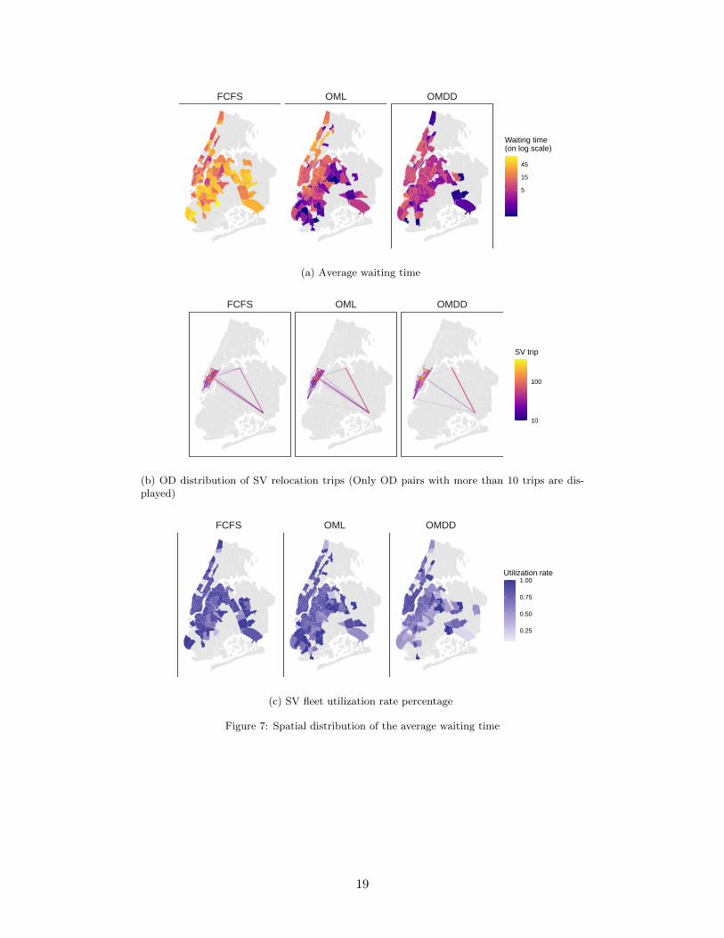
Figure 6 demonstrates the temporal dynamics of the average waiting time in the CaaS systemfrom 5 AM to 12 AM, and Figure 7 shows the spatial distribution of system performances acrossthe study area. For the hourly average waiting time in Figures 6a, we observe three notable surgesin the average waiting time at around 8 AM, 3 PM, and 7 PM, which are associated with theincrease in charging requests as shown in Figure 6c. We note that the 3 PM demand peak for theOML and OMDD policies is not observed in the original charging demand distribution in Figure 3c.Instead, it is the result of the altered system dynamics with the delayed service of charging requestsin previous time steps. For the FCFS policy, a steady increase in average waiting time emergesafter the morning peak and continues until 8 PM, which is the result of the persistent rollover ofunsatisfied charging requests caused by myopic dispatching decisions. The OML policy shows asignificant disparity between peak and off-peak periods, with off-peak waiting time being less than5 minutes and peak-hour waiting time exceeding 20 minutes. On the contrary, the OMDD policy isfound to reach more consistent performances under the shorter surge in charging requests. And theperformance during morning peak hours is comparable to the off-peak periods. The performancesdeteriorate during the evening peak due to higher demand level and longer duration but are stillmore resilient to demand changes than the OML policy with the same number of SVs. Similarobservations can be identified based on the average waiting time’s spatial distribution, as shownin Figure 7a. The FCFS policy is found to be worse than the other two alternatives, with the

17

average waiting time over 15 minutes in almost all taxi zones. The performances are better in highdemand areas such as Manhattan but are considerably worse in other places. Both OMDD andOML policies are able to achieve comparable performances in and outside Manhattan because ofthe optimization performed at the system level. We also note that the average waiting time of theOMDD policy is notably better than the OML policy within high demand areas, and this can beexplained by the fundamental differences of the dispatching philosophies as highlighted in Figure 7b.Specifically, the OMDD shows more clustered relocation trips within Manhattan and much fewerback and forth relocation trips between Manhattan and other areas such as the JFK airport thanthe other two policies. This attributes to the implemented dynamic detour strategy, which reducesrelocation distance by inserting nearby requests between existing charging and often divides onelong relocation trip into multiple short segments to fulfill more charging requests. Meanwhile, theOML policy makes one-shot relocation decisions for the SVs that frequently lead to relocation tripsbetween high and low demand areas, with an example of more OD connections between Manhattanand the JFK airport in Figure 7b. As a consequence, the SV fleet utilization rates of the FCFSand the OML policies are much higher than the OMDD in taxi zones outside Manhattan, as canbe seen in Figure 7c). In the majority of the cases, the SVs in these zones will be immediately sentback to Manhattan under the OML and FCFS policies under the one-step decision making. But theOMDD policy tends to set aside these vehicles and look for alternate SVs in other zones throughthe multi-step optimal relocation strategy. This helps to avoid a significant number of unnecessaryrelocation trips, with a notable example of the much lower utilization rate at JFK airport underthe OMDD policy.

The advantage of the OMDD policy is also captured by the changes in the average relocationdistance, as shown in Figure 6b. Before 8 AM, the average relocation distance starts with highinitial values for the OMDD and OML policies (4 and 4.7 miles) as the charging requests aremore sparsely distributed spatially, hence requiring longer relocation trips and exhibiting feweropportunities for the dynamic detour of the OMDD policy. The FCFS, on the other hand, startswith a short average distance as a result of assigning the nearest available SVs to the chargingrequests under relatively low charging demand. And its relocation distance starts to increase andremain at a higher level during the day due to insufficient supply, which may no longer sustain theshort distance even for the nearest available SVs. The OML policy also shows a similar relocationdistance as the FCFS policy. The reason is because of more frequent back and forth relocation forimmediate available SVs. However, the OMDD policy provides a better solution to mitigate theback and forth relocation issue with its dynamic detour feature and its ability to coordinate amongthe entire SV fleet.

18

FCFS OML OMDD

5

15

45

Waiting time(on log scale)

(a) Average waiting time

FCFS OML OMDD

10

100

SV trip

(b) OD distribution of SV relocation trips (Only OD pairs with more than 10 trips are dis-played)

FCFS OML OMDD

0.25

0.50

0.75

1.00Utilization rate

(c) SV fleet utilization rate percentage

Figure 7: Spatial distribution of the average waiting time

19

FCFS OML OMDD

8 12 16 20 8 12 16 20 8 12 16 200

10000

20000

30000

0.00

0.25

0.50

0.75

1.00

Hour of the day

Cou

ntS

V utilization rate

Waiting time (min) [0,5] (5,10] (10,30] (30,Inf]

Figure 8: Stacked histogram of charging demand by waiting time

To further demonstrate the performances of different policies during peak hours, we dividethe waiting time of the charging requests into four groups and plot the stacked histogram alongwith the corresponding SV fleet utilization rate in Figure 8. The distributions of waiting timeare significantly different during peak hours for the OMDD and OML policies. The OML policyis found to serve a number of charging requests within 5 minutes but also keeps many chargingrequests waiting for more than 30 minutes. This is less of a problem during off-peak periods. But itraises a major concern when there is an undersupply of SVs in prime time, where excessive leftoverrequests are generated and lead to the snowballing of waiting time. This can also be confirmed bythe distribution of served charging requests shown in Figure 6c. The OMDD, on the other hand,is found to adapt to demand surge at the morning peak (8- 10 AM) and minimize the number ofrollover requests during the evening peak (7 - 10 PM). And this is the result of better utilizationof the SV fleet during peak hours and the saving of supply resources before the arrival of the peakhours, as reflected by the change of SV utilization rate for the three policies.

3.4. Service fairness

We are not only interested in the average metrics of the system performances but also thefairness of the CaaS regarding both demand and supply sides of the system. To this end, weintroduce Gini coefficients [44] to evaluate the spatial equity in terms of the differences of averagewaiting time over all taxi zones and the disparity of charging requests served by individual SVs.The calculation for the Gini coefficient is formulated as follows:

G =

∑i

∑j

∣∣∣twi − twj ∣∣∣2n2tw

(18)

where twi is the average waiting time for zone i. n is the total number of zones, and tw is themean value of the average waiting time of all zones. Similarly, we can perform equity analysis onserved requests per SV by replacing twi with the served charging requests for SV i.

20

0.00.10.20.30.40.5

150 300 450SV fleet size

Gin

i coe

ffici

ent

FCFS OMDD OML

(a) Gini coefficients of average zonal waiting time

0.0

0.1

0.2

0.3

0.4

150 300 450SV fleet size

Gin

i coe

ffici

ent

FCFS OMDD OML

(b) Gini coefficients of served charging requests per SV

Figure 9: CaaS performance on equity issues

The results of the Gini coefficients are summarized in Figure 9. For average waiting time, wereport that the Gini coefficient increases with the SV fleet size (up to 500 SVs), and the Ginicoefficient exceeds 0.3 with a fleet greater than 250 in all three policies. The increase of the Ginicoefficient is due to the migration of the system state with all zones having long waiting time tothe reduction of waiting time in certain zones, which is expected to decrease with further increasein SV fleet size as all zones receiving low waiting time. For the FCFS and OML policies, the surgeof charging demand during peak hours motivates additional SVs to flow towards the high-demandareas, leading to an unbalanced SV fleet distribution. As a consequence, the waiting time in high-demand zones and zones close to the high-demand region is expected to be lower than in otherareas on average. We note that the Gini coefficient of both FCFS and OMDD policies is lowerthan that of the OML policy. Nevertheless, the lower Gini coefficient for FCFS is because of theconsistently worse performances over the entire study area, which is precisely the opposite of thereason for the lower Gini coefficient of the OMDD policy.

As for the served requests per SV, the fairness of the assigned requests is vital for the CaaSsystem depending on the ownership of the SVs and how the SVs are operated. In the case ofindividually owned and operated SVs, the fairness of the dispatching policy is critical as it directlylinks to the SV drivers’ workload and salary. As shown in Figure 9b, we also observe that the Ginicoefficient increases with more number of SVs. The initial low Gini coefficient is due to the lackof supply across all time periods, and all SVs are overloaded with charging requests. The FCFSpolicy is found to have the worst Gini coefficient with more SVs as a result of its nearest dispatchingpolicy. Under the FCFS policy, SVs in the high demand tend to stay in these areas, which alsoapplies to those in low demand areas, so that SVs in high demand areas will receive more requestswith relatively shorter relocation trips. Despite the superior performances of the OMDD policy atthe system level, it results in a consistently higher Gini coefficient than the OML policy, which isa side-effect of the dynamic detour strategy. Though the OML is making more relocation trips,it also ensures all SVs similar number of charging requests since it only focuses on immediatelyavailable SVs. On the other hand, as discussed in the previous section, the OMDD will generateclustered short trips in high demand areas, which will likely assign multiple requests with shortrelocation trips for some of the SVs while setting other SVs in the idle state. This represents amajor barrier to implementing the OMDD policy when the SVs are owned by individual drivers,despite its superior system-level efficiency.

21

3.5. CaaS system benefits

After discussing the operation dynamics, we next present the overall benefits of the CaaS systemfor the MaaS industry compared to the adoption of FCSs. And we focus on the CaaS system benefitsin terms of the savings in the OoS time, the relocation distance, and the financial sustainability ofthe CaaS.

−200

−100

0

100

150 300 450SV fleet size

Sav

ing

of O

oS ti

me

FCFS OMDD OML

(a) Savings in OoS time (min per charging request)

0

25

50

75

150 300 450SV fleet size

Sav

ing

of d

ista

nce

FCFS OMDD OML

(b) System savings in relocation distance (mile per min)

Figure 10: CaaS system savings

Figure 10a indicates the savings of OoS time between the CaaS and charging through FCSs. Allmetrics from the CaaS are converted under the FCE consideration to make the results comparableunder the same level of charging demand. The results show that the CaaS achieves consistentsavings with a sufficient number of SVs (>250) for all three policies. In particular, the chargingrequests under the OML and OMDD policies receive similar and most considerable savings at over4 minutes per charging request. Under the FCFS policy, the saving plateaus at 3 min with an SVfleet size larger than 300. The savings are lower than those under the OMDD and the OML, whichis also evidenced in the hourly average waiting time in Figure 5a. The saving will lead to moreserved trips in the MaaS and is critical for promoting a wide adoption of EVs in the MaaS industry.

Figure 10b presents the system savings in travel distance due to the shift from charging atFCSs to the CaaS. The LDEV’s relocation distance to the nearest FCS is assumed to be 15 mileson average. The saving of distance for charging under the OMDD policy remains at a high level ofover 50 miles per minute, followed by the savings of the OML between 10 to 26 miles per minute.The savings of the OMDD policy can be translated into more than 5700 miles per day from 5 AM to12 AM. The FCFS is found to achieve the highest saving in charging miles with a sufficient numberof SVs, as the requests are assigned to the nearest SVs in sequence. For the OML, the saving alsoincreases with more number of SVs since it increases the density of the SVs and naturally reducesthe distance to reach the charging request. On the other hand, the OMDD policy reaches thehighest saving at the fleet size of 175 but will have to trade the savings in charging distance forthe reduction in average waiting time with a larger fleet. As a consequence, the CaaS also markssignificant savings of energy in charging the large-scale LDEVs of the MaaS industry.

22

service price=10 $/time

labor cost=0 $/request

service price=10 $/time

labor cost=1.5 $/request

service price=10 $/time

labor cost=3 $/request

service price=7.5 $/time

labor cost=0 $/request

service price=7.5 $/time

labor cost=1.5 $/request

service price=7.5 $/time

labor cost=3 $/request

service price=5 $/time

labor cost=0 $/request

service price=5 $/time

labor cost=1.5 $/request

service price=5 $/time

labor cost=3 $/request

150 300 450 150 300 450 150 300 450

−50

0

50

−50

0

50

−50

0

50

SV fleet size

Pro

fit (

$/m

in)

FCFS OMDD OML

Figure 11: CaaS system profit ($ per min)

While demonstrating promising contributions to save OoS and charging distance, the feasibilityof the CaaS depends highly on its financial sustainability. We conduct a sensitivity analysis on theprofit level of CaaS with respect to the service price and the labor cost per charging request, and theresults are shown in Figure 11. In general, we find that the service price contributes significantly tothe profit and CaaS users are willing to pay the extra to enjoy a higher level-of-service as comparedto charging at FCSs. Besides, the labor cost also acts as a deterministic factor that affects theprofit level, with the increase in labor cost resulting in a steep reduction of service profit. For thegiven service price and labor cost, the profit resembles a concave function with respect to the SVfleet size, and expanding the SV fleet for reduced average waiting time beyond an optimal fleetsize will not square the additional capital and operation cost for the CaaS. And this optimal fleetsize is found to shift to the left with increasing labor cost and shift to the right with higher serviceprice per charging request. In this regard, for a CaaS startup with a limited initial budget, a highersalary paid to the SV drivers means fewer funds to enlarge the SV fleet size, which then translatesinto less saving of relocation time and higher waiting time of the served LDEVs. On the other

23

hand, a reduced labor cost would benefit the CaaS to gain a higher budget for a larger SV fleet,achieve better service levels, and ensure sustainable cash flow with improved profit levels. A specialcase is the $0 labor cost, which can be achieved through an automated CaaS system, and this caseperforms considerably better than other cases in terms of financial sustainability. And this resulthighlights the autonomous MBU delivery service as an important component for a sustainable CaaSsystem.

Additional insights into the CaaS operation dynamics are observed by inspecting the profitchanges with different configurations of the SV fleet under three dispatching strategies. Thesetrends of the profit can be interpreted by two main components, as indicated in equation ??. Thefirst component is the capital and operation cost corresponding to the increase in SV fleet size, andthe other component is the revenue from the potential CaaS users based on the service level withmore SVs introduced to the fleet. Despite performing worse than the OMDD policy at the systemlevel, the OML policy outperforms the OMDD for a higher system profit with a smaller fleet size(e.g., NSV < 350). In this case, the OML serves more LDEVs with a shorter waiting time, whichleads to a higher turnout rate for using the CaaS and, therefore, more revenues.

As the SV fleet size exceeds 400, the profit under the OMDD policy slightly outperforms theOMDD as it offers a similar service level at the cost of fewer relocation miles. Based on theprofit analyses, we conclude that the CaaS is a potentially profitable business under appropriateservice price, labor cost, fleet size, and dispatching policy configuration. Moreover, despite a lossof revenue, more SVs will yield a higher saving of OoS time, which may well justify the reducedprofit with more served trips in the MaaS industry.

4. Conclusion and Future work

In this paper, we propose the HABM to simulate the CaaS system dynamics, where SV fleetare dispatched to provide on-demand MBU delivery for the LDEVs in the MaaS industry. And weinvestigate the applicability and effectiveness of the CaaS system under three different dispatchingstrategies. The performances of the CaaS framework are validated through comprehensive numer-ical experiments following the same trip dynamics in the NYC taxi market where all taxis areassumed to be replaced with the LDEVs. The CaaS system is found to achieve high level of serviceand satisfy over 95 % charging requests from the LDEVs in NYC with an SV fleet size of 250. Andthe CaaS system has the potential to achieve significant savings in OoS time and charging milesand maintain its financial sustainability under appropriate fleet and price settings.

Based on the analyses of the operation performances, system benefits, and financial sustain-ability, we summarize our recommendation of the CaaS system configurations considering differenttypes of stakeholders as follows:

• TNCs: TNCs such as Uber and Lyft are considered large-scale operators aiming to providea high level of service to their LDEV fleet and prioritize short waiting time and savings inOoS. The OMDD policy is recommended for TNCs with their own SV fleet, while the OMLpolicy is more applicable if the TNCs decide to operate the SVs through crowd-sourcing. Inthis regard, the applicable SV fleet size can be shifted to the right of the profit-maximizationones, which will gain slightly lower profits but achieves less waiting time and more savings ofOoS duration. The loss of profit in the CaaS is likely to be compensated for through extragains from their trip services via the LDEV fleet.

• Small startups as independent CaaS providers: Small startups operate CaaS with a budgetconstraint will need to balance labor costs and the investment into SVs to get the most

24

profits. In this case, the OML protocol can be adopted, and the optimal number of SVs maybe directly applicable to small startups who run CaaS for maximizing revenue.

• State agencies that focus on environmental impact: The priority for these agencies is to reduceemission and energy consumption. They tend to discourage additional travel distances fromthe CaaS sector. In this study, the savings of travel distance under the OMDD doubles thoseunder the OML. As a result, the agencies may consider subsidizing small startups to runthe OMDD strategy or subsidize potential CaaS users for accepting a higher average waitingtime.

While the study represents an initial attempt to investigate the dynamics of the CaaS system,it opens up several future research opportunities to advance our understanding of an optimallydeployed CaaS system. First, the multi-depot setting can be investigated to improve the servicelevel. Also, incentives and dynamic service price may motivate additional SVs to get out of thehigh-density area (e.g., Manhattan) to serve the LDEVs in other areas during peak hours so as toimprove the unbalanced level of service in the city. In addition to the MaaS industry, the proposedCaaS system can also be extended to other micro-mobility sectors as a battery delivery service,e.g., the shared electric scooters, the electric bikes, and the electric commercial delivery drones.These scenarios describe a lite MBU delivery service under more uncertain trip trajectories andwill require additional considerations to tailor to the unique features of these systems.

References

[1] International Energy Agency. Global EV Outlook 2020, 2020.

[2] Xinwu Qian, Tian Lei, Jiawei Xue, Zengxiang Lei, and Satish V Ukkusuri. Impact of trans-portation network companies on urban congestion: Evidence from large-scale trajectory data.Sustainable Cities and Society, 55:102053, 2020.

[3] Assessing ride-hailing company commitments to electrification. https://theicct.org/

publications/ridehailing-electrification-commitment. Accessed: 2020, July.

[4] Alternative fueling station locator. https://afdc.energy.gov/stations/#/find/nearest.Accessed: 2019, July.

[5] Privacy & legal | Tesla. https://www.tesla.com/about/legal?#supercharger-fair-use,Accessed on 7 October 2020.

[6] Zheng Dong, Cong Liu, Yanhua Li, Jie Bao, Yu Gu, and Tian He. Rec: Predictable chargingscheduling for electric taxi fleets. In 2017 IEEE Real-Time Systems Symposium (RTSS), pages287–296. IEEE, 2017.

[7] Fang He, Di Wu, Yafeng Yin, and Yongpei Guan. Optimal deployment of public chargingstations for plug-in hybrid electric vehicles. Transportation Research Part B: Methodological,47:87–101, 2013.

[8] Fang He, Yafeng Yin, and Siriphong Lawphongpanich. Network equilibrium models withbattery electric vehicles. Transportation Research Part B: Methodological, 67:306–319, 2014.

[9] Fang He, Yafeng Yin, and Jing Zhou. Deploying public charging stations for electric vehicleson urban road networks. Transportation Research Part C: Emerging Technologies, 60:227–240,2015.

25

[10] Raffaela Riemann, David ZW Wang, and Fritz Busch. Optimal location of wireless chargingfacilities for electric vehicles: flow-capturing location model with stochastic user equilibrium.Transportation Research Part C: Emerging Technologies, 58:1–12, 2015.

[11] Zhibin Chen, Fang He, and Yafeng Yin. Optimal deployment of charging lanes for electricvehicles in transportation networks. Transportation Research Part B: Methodological, 91:344–365, 2016.

[12] Zhibin Chen, Wei Liu, and Yafeng Yin. Deployment of stationary and dynamic charginginfrastructure for electric vehicles along traffic corridors. Transportation Research Part C:Emerging Technologies, 77:185–206, 2017.

[13] Chengzhang Wang, Fang He, Xi Lin, Zuo-Jun Max Shen, and Meng Li. Designing locations andcapacities for charging stations to support intercity travel of electric vehicles: An expandednetwork approach. Transportation Research Part C: Emerging Technologies, 102:210–232,2019.

[14] Yi He, Ziqi Song, and Zhaocai Liu. Fast-charging station deployment for battery electric bussystems considering electricity demand charges. Sustainable Cities and Society, 48:101530,2019.

[15] Yuping Lin, Kai Zhang, Zuo-Jun Max Shen, Bin Ye, and Lixin Miao. Multistage large-scalecharging station planning for electric buses considering transportation network and power grid.Transportation Research Part C: Emerging Technologies, 107:423–443, 2019.

[16] Jie Yang, Jing Dong, and Liang Hu. A data-driven optimization-based approach for siting andsizing of electric taxi charging stations. Transportation Research Part C: Emerging Technolo-gies, 77:462–477, 2017.

[17] Rui Chen, Xinwu Qian, Lixin Miao, and Satish V Ukkusuri. Optimal charging facility loca-tion and capacity for electric vehicles considering route choice and charging time equilibrium.Computers & Operations Research, 113:104776, 2020.

[18] Ho-Yin Mak, Ying Rong, and Zuo-Jun Max Shen. Infrastructure planning for electric vehicleswith battery swapping. Management Science, 59(7):1557–1575, 2013.

[19] Yu Zheng, Zhao Yang Dong, Yan Xu, Ke Meng, Jun Hua Zhao, and Jing Qiu. Electricvehicle battery charging/swap stations in distribution systems: comparison study and optimalplanning. IEEE transactions on Power Systems, 29(1):221–229, 2013.

[20] Mushfiqur R Sarker, Hrvoje Pandzic, and Miguel A Ortega-Vazquez. Optimal operation andservices scheduling for an electric vehicle battery swapping station. IEEE transactions onpower systems, 30(2):901–910, 2014.

[21] Bo Sun, Xiaoqi Tan, and Danny HK Tsang. Optimal charging operation of battery swap-ping stations with QoS guarantee. In 2014 IEEE International Conference on Smart GridCommunications (SmartGridComm), pages 13–18. IEEE, 2014.

[22] Yang Wang, Wenjian Ding, Liusheng Huang, Zheng Wei, Hengchang Liu, and John AStankovic. Toward urban electric taxi systems in smart cities: The battery swapping challenge.IEEE Transactions on Vehicular Technology, 67(3):1946–1960, 2017.

26

[23] Shisheng Huang, Liang He, Yu Gu, Kristin Wood, and Saif Benjaafar. Design of a mobilecharging service for electric vehicles in an urban environment. IEEE Transactions on IntelligentTransportation Systems, 16(2):787–798, 2014.

[24] Huwei Chen, Zhou Su, Yilong Hui, and Hui Hui. Optimal approach to provide electric vehicleswith charging service by using mobile charging stations in heterogeneous networks. In 2016IEEE 84th Vehicular Technology Conference (VTC-Fall), pages 1–5. IEEE, 2016.

[25] Sujie Shao, Shaoyong Guo, and Xuesong Qiu. A mobile battery swapping service for electricvehicles based on a battery swapping van. Energies, 10(10):1667, 2017.

[26] Portable Chargers – SparkCharge Portable Ultra-Fast EV Charging. https://sparkcharge.io/portable-chargers/. Accessed: 2020, October 3.

[27] Alternative Fuels Data Center: Developing Infrastructure to Charge Plug-In Electric Vehi-cles. https://afdc.energy.gov/fuels/electricity_infrastructure.html, Accessed on10 November 2020.

[28] Margaret Smith and Johnathan Castellano. Costs associated with non-residential electricvehicle supply equipment: Factors to consider in the implementation of electric vehicle chargingstations. Technical report, 2015.

[29] Jeffrey Lidicker, Timothy Lipman, and Brett Williams. Business model for subscription ser-vice for electric vehicles including battery swapping, for san francisco bay area, california.Transportation research record, 2252(1):83–90, 2011.

[30] Mobi EV charger, FreeWire Technologies. https://freewiretech.com/products/mobi-ev/.Accessed: 2020, June 15.

[31] Building EV charging solutions for landlords, consumers, and automakers. https://www.

evpassport.com/.

[32] EVgo charging plans — How much does it cost to charge an EV. https://www.evgo.com/.

[33] GM unveils a new electric vehicle platform and battery in bidto take on Tesla. https://www.theverge.com/2020/3/4/21164513/

gm-ev-platform-architecture-battery-ultium-tesla. Accessed: 2020, October3.

[34] Icograms Templates - create beautiful isometric diagrams, infographics and illustrations fromtemplates. https://icograms.com/templates.php, Accessed on 10 October 2020.

[35] Xinwu Qian, Jiawei Xue, Stanislav Sobolevsky, Chao Yang, and Satish Ukkusuri. StationarySpatial Charging Demand Distribution for Commercial Electric Vehicles in Urban Area. In2019 IEEE Intelligent Transportation Systems Conference (ITSC), pages 220–225. IEEE, 2019.

[36] Harold W Kuhn. The Hungarian method for the assignment problem. Naval research logisticsquarterly, 2(1-2):83–97, 1955.

[37] Michael Lammert and Kevin Walkowicz. Eighteen-month final evaluation of UPS secondgeneration diesel hybrid-electric delivery vans. Technical report, National Renewable EnergyLab.(NREL), Golden, CO (United States), 2012.

27

[38] Kenneth E Train. Discrete choice methods with simulation. Cambridge university press, 2009.

[39] National Research Council et al. Technologies and approaches to reducing the fuel consumptionof medium-and heavy-duty vehicles. National Academies Press, 2010.

[40] 2013 NYC yellow taxi trip record data. https://www1.nyc.gov/site/tlc/about/

tlc-trip-record-data.page. Accessed: March, 2019.

[41] New York City Taxi and Limousine Commission. Aggregated Reports. https://www1.nyc.

gov/site/tlc/about/aggregated-reports.page, Accessed on November 2020.

[42] Katrin Seddig, Patrick Jochem, and Wolf Fichtner. Integrating renewable energy sources byelectric vehicle fleets under uncertainty. Energy, 141:2145–2153, 2017.

[43] NYC Investment Sales — Land Prices New York. https://therealdeal.com/issues_

articles/new-york-city-land-prices/, Accessed: 2020, November 19.

[44] Corrado Gini. Variabilita e mutabilita. Reprinted in Memorie di metodologica statistica (Ed.Pizetti E, Salvemini, T). Rome: Libreria Eredi Virgilio Veschi, 1912.

28