charge and discharge of a capacitor · charging and discharging of the capacitor, we are interested...

Charge and Discharge of a Capacitor

INTRODUCTION

Capacitors1 are devices that can store electric charge and energy. Capacitors have several uses,such as filters in DC power supplies and as energy storage banks for pulsed lasers. Capacitors passAC current, but not DC current, so they are used to block the DC component of a signal so thatthe AC component can be measured. Plasma physics2 makes use of the energy storing ability ofcapacitors. In plasma physics short pulses of energy at extremely high voltages and currents arefrequently needed. A capacitor can be slowly charged to the necessary voltage and then dischargedquickly to provide the energy needed. It is even possible to charge several capacitors to a certainvoltage and then discharge them in such a way as to get more voltage (but not more energy) outof the system than was put in.

This experiment features an RC circuit, which is one of the simplest circuits that uses a capaci-tor. You will study this circuit and ways to change its effective capacitance by combining capacitorsin series and parallel arrangements.

DISCUSSION OF PRINCIPLES

A capacitor consists of two conductors separated by a small distance. When the conductors areconnected to a charging device (for example, a battery), charge is transferred from one conductorto the other until the difference in potential between the conductors due to their equal but oppositecharge becomes equal to the potential difference between the terminals of the charging device.The amount of charge stored on either conductor is directly proportional to the voltage, and theconstant of proportionality is known as the capacitance3. This is written algebraically as

Q = C∆V. (1)

The charge C is measured in units of coulomb (C), the voltage ∆V in volts (V), and the capacitanceC in units of farads (F). Capacitors are physical devices; capacitance is a property of devices.

Charging and Discharging

In a simple RC circuit4, a resistor and a capacitor are connected in series with a battery and aswitch. See Fig. 1.

1http://en.wikipedia.org/wiki/Capacitor2http://en.wikipedia.org/wiki/Plasma (physics)3http://en.wikipedia.org/wiki/Capacitance4http://en.wikipedia.org/wiki/RC circuit

c©2012 Advanced Instructional Systems, Inc. and North Carolina State University 1

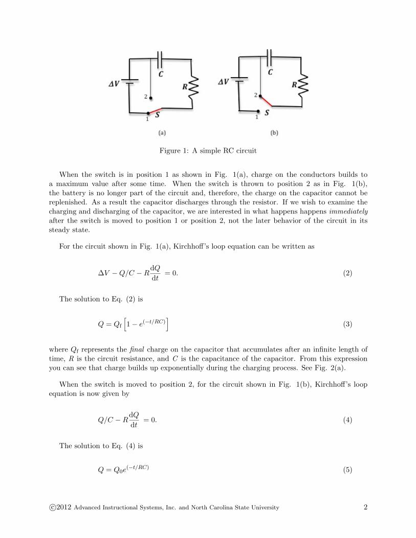
Figure 1: A simple RC circuit

When the switch is in position 1 as shown in Fig. 1(a), charge on the conductors builds toa maximum value after some time. When the switch is thrown to position 2 as in Fig. 1(b),the battery is no longer part of the circuit and, therefore, the charge on the capacitor cannot bereplenished. As a result the capacitor discharges through the resistor. If we wish to examine thecharging and discharging of the capacitor, we are interested in what happens happens immediatelyafter the switch is moved to position 1 or position 2, not the later behavior of the circuit in itssteady state.

For the circuit shown in Fig. 1(a), Kirchhoff’s loop equation can be written as

∆V −Q/C −RdQ

dt= 0. (2)

The solution to Eq. (2) is

Q = Qf

[1 − e(−t/RC)

](3)

where Qf represents the final charge on the capacitor that accumulates after an infinite length oftime, R is the circuit resistance, and C is the capacitance of the capacitor. From this expressionyou can see that charge builds up exponentially during the charging process. See Fig. 2(a).

When the switch is moved to position 2, for the circuit shown in Fig. 1(b), Kirchhoff’s loopequation is now given by

Q/C −RdQ

dt= 0. (4)

The solution to Eq. (4) is

Q = Q0e(−t/RC) (5)


where Q0 represents the initial charge on the capacitor at the beginning of the discharge, i.e., att = 0. You can see from this expression that the charge decays exponentially when the capacitordischarges, and that it takes an infinite amount of time to fully discharge. See Fig. 2(b).

Figure 2: Change versus time graphs

Time Constant τ

The product RC (having units of time) has a special significance; it is called the time constantof the circuit. The time constant is the amount of time required for the charge on a chargingcapacitor to rise to 63% of its final value. In other words, when t = RC,

Q = Qf

(1 − e−1

)(6)

and

1 − e−1 = 0.632. (7)

Another way to describe the time constant is to say that it is the number of seconds required forthe charge on a discharging capacitor to fall to 36.8% (e−1 = 0.368) of its initial value.

We can use the definition(I = dQ

dt

)of current through the resistor and Eq. (3) and Eq. (5) to

get an expression for the current during the charging and discharging processes.

charging: I = +I0e−t/RC (8)

discharging: I = −I0e−t/RC (9)

where I0 = ∆VfR in Eq. (8) and Eq. (9) is the maximum current in the circuit at time t = 0.


Then the potential difference across the resistor will be given by the following.

charging: ∆V = +∆Vfe−t/RC (10)

discharging: ∆V = −∆V0e−t/RC (11)

Note that during the discharging process the current will flow through the resistor in the oppositedirection. Hence I and ∆V in Eq. (9) and Eq. (11) are negative. This voltage as a function oftime is shown in Fig. 3.

Figure 3: Voltage across the resistor as a function of time

It is useful to describe charging and discharging in terms of the potential difference between theconductors (i.e., “the voltage across the capacitor”), since the voltage across a capacitor can bemeasured directly in the lab. By using the relationship Q = C∆V, Eq. (3) and Eq. (5) that describethe charging and discharging of a capacitor can be rewritten in terms of the voltage. Merely divideboth equations by C, and the relationships become the following.

charging: ∆V = ∆Vf

[1 − e(−t/RC)

](12)

discharging: ∆V = ∆V0e(−t/RC) (13)

Note that these two equations are similar in form to Eq. (3) and Eq. (5). The graph of the voltageacross the capacitor versus time is shown in Fig. 4 below.


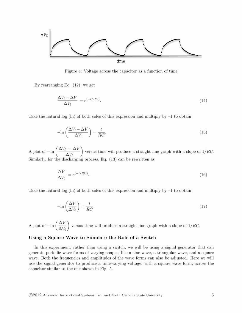
Figure 4: Voltage across the capacitor as a function of time

By rearranging Eq. (12), we get

∆Vf − ∆V

∆Vf= e(−t/RC). (14)

Take the natural log (ln) of both sides of this expression and multiply by –1 to obtain

−ln

(∆Vf − ∆V

∆Vf

)=

t

RC. (15)

A plot of −ln

(∆Vf − ∆V

∆Vf

)versus time will produce a straight line graph with a slope of 1/RC.

Similarly, for the discharging process, Eq. (13) can be rewritten as

∆V

∆V0= e(−t/RC). (16)

Take the natural log (ln) of both sides of this expression and multiply by –1 to obtain

−ln

(∆V

∆V0

)=

t

RC. (17)

A plot of −ln

(∆V

∆V0

)versus time will produce a straight line graph with a slope of 1/RC.

Using a Square Wave to Simulate the Role of a Switch

In this experiment, rather than using a switch, we will be using a signal generator that cangenerate periodic wave forms of varying shapes, like a sine wave, a triangular wave, and a squarewave. Both the frequencies and amplitudes of the wave forms can also be adjusted. Here we willuse the signal generator to produce a time-varying voltage, with a square wave form, across thecapacitor similar to the one shown in Fig. 5.


Figure 5: A square wave with period T

The output voltage from the signal generator changes back and forth from a constant positivevalue to a constant zero volts in equal intervals of time t. The time T = 2t is the period of thesquare wave. During the first half of the cycle, when the voltage is positive, it is similar to theswitch being in position 1. During the second half of the cycle, when the voltage is zero, it is thesame as the switch being in position 2. So the square wave, which is a DC voltage that is turnedon and off periodically, serves as both battery and switch in the setup in Fig. 1.

The signal generator allows this switching to be done repeatedly, and it is possible to optimizethe data collection by adjusting the frequency of the repetition. This frequency will depend on thetime constant of the RC circuit.

When the time t is larger than the time constant τ of the RC circuit, the capacitor will haveenough time to charge and discharge, and the voltage across the capacitor will be as shown inFig. 4.

OBJECTIVE

In this experiment a (computer-emulated) oscilloscope5 will be used to monitor the potentialdifference, and thus, indirectly, the charge on a capacitor. The voltage measurements will be used intwo different ways to compute the time constant of the circuit. Finally, capacitors will be connectedin parallel to examine their equivalent circuit capacitance.

EQUIPMENT

PASCO circuit board

Signal interface with power output

Connecting wires

DataStudio software

PROCEDURE

Please print the worksheet for this lab. You will need this sheet to record your data.

Setting Up the RC Circuit

The RLC circuit board that you will be using consists of three resistors and two capacitorsamong other elements. See Fig. 6 below. In theory you can, therefore, have different combinations

5http://en.wikipedia.org/wiki/Oscilloscope


of resistors and capacitors. In this experiment you will use the 33-Ω and 100-Ω resistors and thetwo capacitors.

Figure 6: RLC circuit board

1 Connect the far right output terminal of the signal interface to the 33-Ω resistor at point 2.

2 To bypass the inductor, connect a wire from point 8 to point 9.

3 Connect point 6 to the second output terminal of the signal interface to complete the circuit.

4 Connect the voltage probe into analog channel A.

5 To measure the voltage across the capacitor connect the black lead of the voltage probe to point6 and the red lead to point 9.

Make sure that the ground of the interface (the “–” lead) is connected to the same side of thecapacitor as the ground of the signal generator (power output).

Your circuit connection should look like that in Fig. 7.

Figure 7: Circuit diagram


CHECKPOINT 1: Ask your TA to check your circuit connections before proceeding.

Procedure A: Time Constant of the Circuit

We will use the computer to emulate the oscilloscope in this experiment.

6 Open the DataStudio file associated with this lab, which starts the DataStudio program. Ascreen similar to Fig. 8 is displayed.

Figure 8: Opening screen of DataStudio file

7 Set the signal generator to produce a positive square wave by highlighting the positive squarewave in the signal generator window as shown in Fig. 9 below.

Figure 9: Signal generator window

8 Set the signal generator to produce a square wave of 5-V amplitude at a frequency of 20 Hz.


9 Turn on the signal generator by clicking ON in the signal generator window.

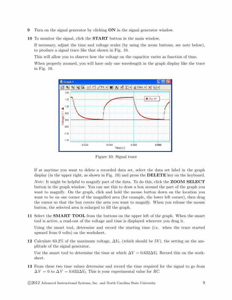
10 To monitor the signal, click the START button in the main window.

If necessary, adjust the time and voltage scales (by using the zoom buttons, see note below),to produce a signal trace like that shown in Fig. 10.

This will allow you to observe how the voltage on the capacitor varies as function of time.

When properly zoomed, you will have only one wavelength in the graph display like the tracein Fig. 10.

Figure 10: Signal trace

If at anytime you want to delete a recorded data set, select the data set label in the graphdisplay (in the upper right, as shown in Fig. 10) and press the DELETE key on the keyboard.

Note: It might be helpful to magnify part of the data. To do this, click the ZOOM SELECTbutton in the graph window. You can use this to draw a box around the part of the graph youwant to magnify. On the graph, click and hold the mouse button down on the location youwant to be on one corner of the magnified area (for example, the lower left corner), then dragthe cursor so that the box covers the area you want to magnify. When you release the mousebutton, the selected area is enlarged to fill the graph.

11 Select the SMART TOOL from the buttons on the upper left of the graph. When the smarttool is active, a read-out of the voltage and time is displayed wherever you drag it.

Using the smart tool, determine and record the starting time (i.e. when the trace startedupward from 0 volts) on the worksheet.

12 Calculate 63.2% of the maximum voltage, ∆Vf, (which should be 5V), the setting on the am-plitude of the signal generator.

Use the smart tool to determine the time at which ∆V = 0.632∆Vf. Record this on the work-sheet.

13 From these two time values determine and record the time required for the signal to go from∆V = 0 to ∆V = 0.632∆Vf. This is your experimental value for RC.


14 On the worksheet, fill in the accepted values for the resistance and the capacitance, which areprinted on the circuit board.

15 Compute the experimental value of the capacitance using your experimental value for RC andthe accepted value of R. Record this on the worksheet.

16 Compute the percent error using the two values for the capacitance. See Appendix B.

CHECKPOINT 2: Ask your TA to check your data and calculations before proceeding.

Procedure B: Calculation of Capacitance by Graphical Methods

17 Record the maximum voltage on the worksheet.

18 From the recorded data, find the times at which ∆V = 1, 2, 3, and 4 volts on the rising partof the curve using the smart tool. Record this information in Data Table 1 on the worksheet.

Note: You might need to zoom in a lot to get the precision you need when using the SmartTool.

19 Perform the necessary calculations to complete Data Table 1.

20 Using Excel, plot −ln(

∆Vf − ∆V∆Vf

)versus time. See Appendix G.

21 Use the linest function in Excel to determine the slope of the line and record this value on theworksheet. See Appendix J.

22 From the value of the slope determine the time constant and the capacitance. Record thesevalues on the worksheet.

23 Compute the percent error between this value of the capacitance and the accepted value.

CHECKPOINT 3: Ask your TA to check your data and calculations before proceeding.

Procedure C: Measuring Effective Capacitance

Capacitance adds directly when capacitors are connected in parallel, and inversely when con-nected in series. This is opposite of the rule for resistors. For capacitors in parallel, the effectivecapacitance is given by

Ceff = C1 + C2 + C3 + ... (18)

and for capacitors in series, the effective capacitance is

1

Ceff=

1

C1+

1

C2+

1

C3+ ... (19)


24 Connect the second capacitor (330 µF) in parallel with the capacitor used in Procedure A byconnecting a wire from point 6 to point 7.

25 Switch the resistor to the 10-Ω resistor by moving the connection from point 2 to point 1.

26 Record another data set by clicking START in the main window.

Once you have recorded the second data set, you might want to display only that data on thegraph and remove data set 1. To do this, delete the first run (see the note in Step 10).

You will be looking at just one wavelength in the graph display.

27 For this part of the experiment you will consider the discharging portion of the curve.

Now the initial voltage ∆V0 will be the highest value of the peak before the graph starts to falloff. Record this value on the worksheet.

28 From the recorded data, find the times at which ∆V = 1, 2, 3, and 4 volts on the falling part ofthe curve using the smart tool. (Note: You might need to zoom in a lot to get the precision youneed when using the smart tool). Record this information in Data Table 2 on the worksheet.

29 Perform the necessary calculations to complete Data Table 2.

30 Using Excel, plot −ln

(∆V

∆V0

)versus time.

31 Use the linest function in Excel to determine the slope of the line and record this value on theworksheet.

32 From the value of the slope determine the time constant and record these values on the work-sheet.

33 Compute Ceff the effective capacitance of the parallel combination using the accepted value forR.

34 Compare this experimental value with that obtained from Eq. (18) and the accepted values ofthe capacitance, by computing the percent error between the two values.

CHECKPOINT 4: Ask to your TA check your data and calculations.


charge and discharge of a capacitor · charging and discharging of the capacitor, we are interested...

Documents