Characterizing Multi-Decadal Variability in the Southeastern United States

Marcus D. WilliamsCenter for Ocean-Atmospheric Prediction Studies

July 2nd 2010

Introduction•To predict future climate variability, and to interpret this variability with appropriate confidence, it is highly desirable to have an understanding of past variability and climate cycles.

•The increased global interest in climate change and its impacts has made the need to understand types of long-term variability more pressing.

•Regional differences exist in climate variability

• Most parts of the world are considered to be warming when examined over a long enough record.

• The Southeastern United States along with parts of Europe and Asia have been identified as outliers

Climate and Florida CitrusAdapted from: John Attaway, “A History of Florida Citrus Freezes”

•Impact Freezes:•February 7-9, 1835•December 29, 1894•February 8, 1895•February 13-14, 1899•December 12-13, 1934•January 27-19, 1940•December 12-13, 1962•January 18-20, 1977•January 12-14, 1981•December 24-25, 1983•January 20-22, 1985•December 24-25, 1989•January 19, 1997

Freeze damaged orange trees in 1895

Present Day – Citrus moves further South

Beginning in 1977 and lasting through 1989, Florida saw a succession of severe freezes that damaged trees further south than ever before.

The center of production moved further south to its present position in west-central and southwest Florida.

The more tropical climate of south Florida bring increased disease threats such as citrus canker and greening along with greater risk of hurricane damage.

Introduction•January 2010 Dover/Plant City Freeze Event

• Eastern Hillsborough county experienced temperatures below 34 degrees for 11 consecutive days

• Farmers pumped large quantities of groundwater in an effort to protect their crops

• Resulted in dropping the aquifer level 60 feet and caused more than 750 dry wells for neighboring homeowners

• Caused several sinkholes in the region, one which closed two lanes of I-4 for a short period

Source: Southwest Florida Water Management District

Introduction

•Easterling et al. 1997•Analyzed monthly averaged min and max temperatures and DTR at 5400 observing stations around the world

•Calculated anomalies from the mean of the base period of 1961 to 1985 for all station in a 5° x 5° lat-lon grid box

•P.O.R. of data for study was from 1950-1993

Introduction

Introduction and Background•In the Southeastern United States (SE US) the El Niño- Southern Oscillation (ENSO) signal is widely recognized as the dominate mode of climate variability.

•Ropelewski and Halpert provided research that showed interannual the impacts of ENSO on temperature and precipitation patterns.

•Work done by the Intergovernmental Panel on Climate Change addresses climate change on interannual to multi-decadal timescales.

Introduction and Background•The analysis presented in this research identifies a mode of variability for the SE US that is of larger magnitude than the trend, and is influential on a multi-decadal timescale.

•Analysis has identified a multi-decadal regime in the long-term temperature records. Not a trend in temperature records

•The multi-decadal regime shifts from periods warmer than normal temperatures, to periods of colder than normal temperatures.

Multidecadal Variability in the SoutheastAlabama Annual Temperature

Multidecadal Variability in the SoutheastAlabama Annual Temperature

Warm period 1920-1957

Cold period 1958-1998

Multidecadal Variability in the Southeast

•Same multi-decadal pattern is displayed in the raw, unadjusted station data

•1920-1957: Warm regime (WR)

•1958-1998: Cold regime (CR)

Warm regime 1920-1957

Cold regime 1958-1998

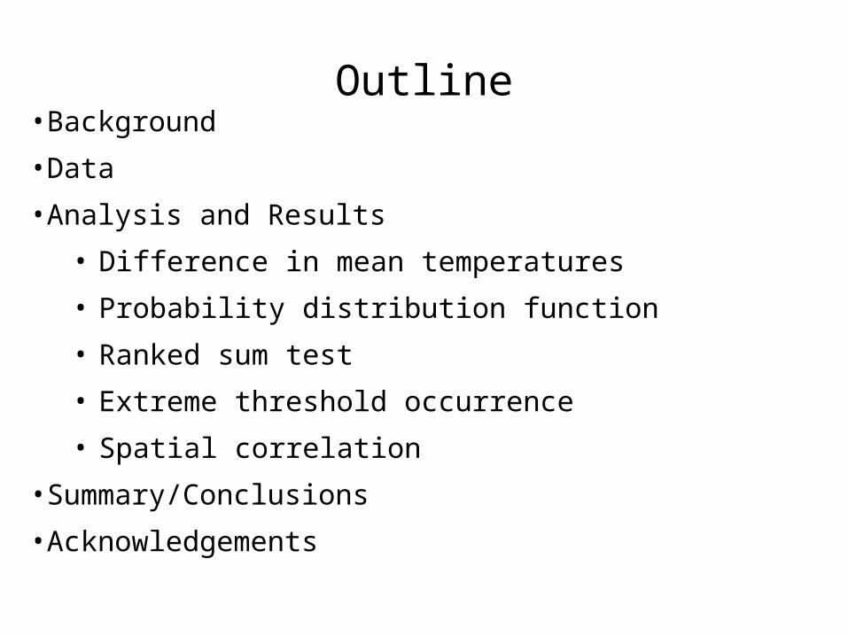
Outline•Background

•Data

•Analysis and Results

• Difference in mean temperatures

• Probability distribution function

• Ranked sum test

• Extreme threshold occurrence

• Spatial correlation

•Summary/Conclusions

•Acknowledgements

Introduction and Background•The mode of climate variability found in my work has been inadequately characterized in the SE US by prior studies

•Often times studies describe variability is in the realm of trend analysis.

•The periods over which the trends are fitted can greatly influence the significance or even the sign of the trends.

• Work done by Lathers and Palecki, Diaz and Quayle, and other have investigated warm and cool periods

• Monthly averages for 344 climate divisions was analyzed

• Many of the studies found the greatest change in summer temperatures

•What’s new?

What’s new•Characterizing a change in temperature regime as opposed to trend analysis

•Warm and Cool periods have been alluded to in the SE US, this study offers comprehensive comparison of a regime shift

•Region of analysis not as broad as other studies

•Single station analyzed as opposed to climate division data

•Daily minimum and maximum temperatures analyzed separately as opposed to annual or monthly averages

•Unadjusted daily min and max values analyses as opposed to bias corrected USHCN data

Data•Data provided by the National Weather Service Cooperative Observation Program (COOP)

•DS 3200 and DS 3206

• DS 3200 is a daily summary of the day data set that consist of 8,000 active observing stations recording daily values of max temp, min temp and precip.

• DS 3206 is the data rescue of the data, converting paper records to digital copies

Data

Station coverage map of the104 stations used in the SE US encompassing the states of Alabama, Florida, Georgia, North Carolina, and South Carolina

Data•Stations have data available dating back to at least 1920 and ending in 2007

•Many of the stations used are part of the United States Historical Climate Network (USHCN)

• However, for the purpose of this study the daily, unadjusted observations are used

•Missing data is addressed by the criteria set forth by Smith (2006)

Data•A multiple linear regression method is used to replace any missing data

•Data are pulled from two to five station that lie within a 50-mile radius

•Data are de-trended and the seasonal cycle is removed.

•Reference stations with correlations of 0.6 or higher are used to calculate the multiple linear regression

Analysis and Results•Goals of my study are to characterize the signal

• seasonality,

• Is the regime shift seasonal in nature, or is it present in all seasons

• spatial extent,

• How coherent is the signal of the regime shift

• temperature extremes

• Is the regime shift affecting the occurrence of extreme temperatures

•Analysis and Results

• Difference in mean temperatures

• Probability distribution function

• Ranked sum test

• Extreme threshold occurrence

• Spatial correlation

Difference in mean temperatures •One of the easiest ways to quantify the differences between the two regimes are to compare the mean temperatures

•For each station the mean temperature for the WR is subtracted from the mean temperature for the CR

• If the difference is negative the station is assigned a blue dot, positive differences get assigned a red dot

• The size of the dot is indicative of the degree difference between the means

•Clear that signal is spatially coherent throughout the SE US

•Signal strongest in winter minimum and maximum temperatures

•Some stations display a difference in means as great as 5F between the two regimes

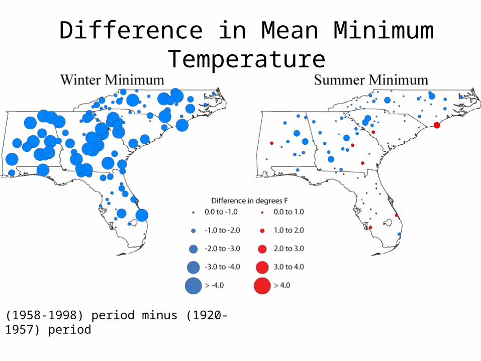
Difference in Mean Minimum Temperature

(1958-1998) period minus (1920-1957) period

Difference in Mean Minimum Temperature

(1958-1998) period minus (1920-1957) period

Difference in Mean Maximum Temperature

(1958-1998) period minus (1920-1957) period

Difference in Mean Maximum Temperature

(1958-1998) period minus (1920-1957) period

Difference in mean temperatures•Two tailed student t-test used to determine if the difference in the means statistically significant

• t =

•Daily min and max temperatures are tested individually for each season

•The t scores calculated where on average large and positive

• Rarely was a positive t score below 2.5, which suggest significance on the 99% confidence level

nn

xx

2

2

1

1

21

varvar

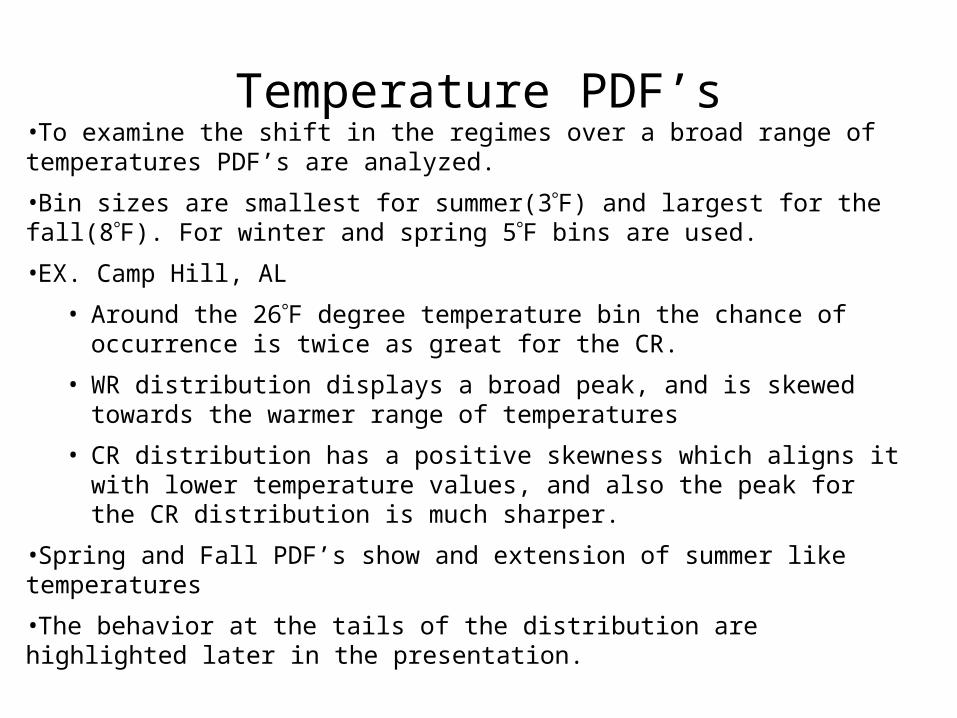
Temperature PDF’s•To examine the shift in the regimes over a broad range of temperatures PDF’s are analyzed.

•Bin sizes are smallest for summer(3F) and largest for the fall(8F). For winter and spring 5F bins are used.

•EX. Camp Hill, AL

• Around the 26F degree temperature bin the chance of occurrence is twice as great for the CR.

• WR distribution displays a broad peak, and is skewed towards the warmer range of temperatures

• CR distribution has a positive skewness which aligns it with lower temperature values, and also the peak for the CR distribution is much sharper.

•Spring and Fall PDF’s show and extension of summer like temperatures

•The behavior at the tails of the distribution are highlighted later in the presentation.

Camp Hill, ALregion

Camp Hill, AL Winter Minimum Temperature Distribution

•20th percentile shifted from 29F (WR) to 23F (CR)

•80th percentile shifted from 47F (WR) to 41F (CR)

Camp Hill, AL Minimum Temperature Distributions

Camp Hill, AL Maximum Temperature Distributions

Chapel Hill, NCregion

Little Mountain, SCregion

Milledgeville, GAregion

Camp Hill, ALregion

Maximum Temperature Distributions

Analysis and Results•All seasons display evidence of a shift between the two regimes for minimum and maximum temperatures

•Shift in distributions are largest in winter minimum temperatures.

•Spring and Fall distributions display an extension of summer like temperatures

•Are the shifts in the distribution statistically significant?

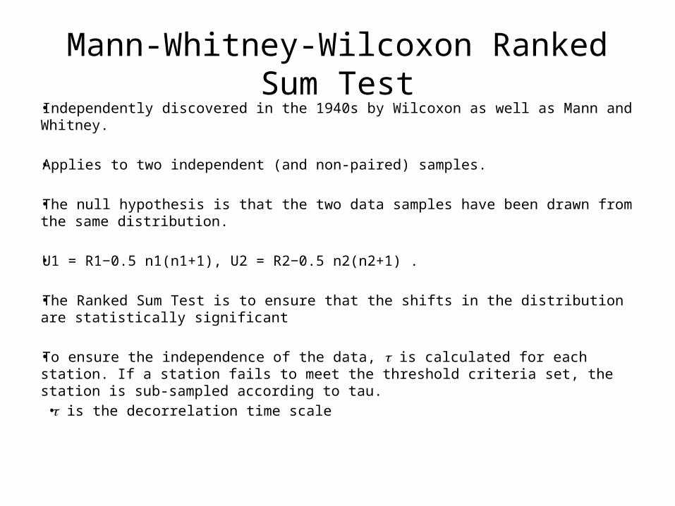
Mann-Whitney-Wilcoxon Ranked Sum Test•Independently discovered in the 1940s by Wilcoxon as well as Mann and Whitney.

•Applies to two independent (and non-paired) samples.

•The null hypothesis is that the two data samples have been drawn from the same distribution.

•U1 = R1−0.5 n1(n1+1), U2 = R2−0.5 n2(n2+1) .

•The Ranked Sum Test is to ensure that the shifts in the distribution are statistically significant

•To ensure the independence of the data, is calculated for each station. If a station fails to meet the threshold criteria set, the station is sub-sampled according to tau.

• is the decorrelation time scale

Ranked sum test•Confidence limits are set on a station by station basis for the rejection of the null hypothesis

•Each Station is assigned a colored symbol corresponding to a range of confidence limits

• Stations with confidence limits 99% are coded red.• Station that lie within the 95-98% confidence interval are yellow• Stations that lie within the 90-94% range are green• Stations <90% are purple

•Overwhelming evidence that distribution are statistically significant for Winter and Summer•Spring and Fall seasons display less confidence than Winter and Summer

Confidence Limit Maps

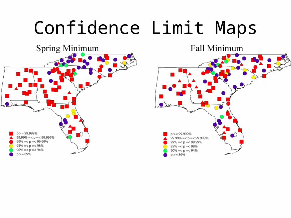
Confidence Limit Maps

Confidence Limit Maps

Confidence Limit Maps

Threshold Occurrence•With the shift displayed in the temperature PDF’s, one would expect an increased occurrence of temperatures at the tails of the distribution

•Thresholds were set at 32F and 95F and counts of occurrences per year where made.

•As expected there was a difference in the occurrence of 32F and 95F between the warm and cold regime.

•Analysis implies that during the WR it was hotter longer

Henderson, NCregion

Henderson, NC Fall Maximum Temperature Distribution

•Largest shift in Fall maximum temps occur around the higher temperature values

•This implies an extension of Summer like temps into the fall season

Threshold occurrence

Three occurrences of

95F or greater for the WR compared to no occurrences for the CR

Talladega, ALregion

Waycross, GA and Lake City, FL

regions

Talladega, AL

•Substantial shift in the number of days temperature reached 95F or higher

12

6

0

Threshold Occurrence

43 days per year temperatures reached 32F or below during the CR compared to 19 for the WR

Waycross, GA Occurrences of 32F or below

Waycross, GA Winter Minimum Temperature Distribution

Lake City, FLLake City ,FL

Occurrences of 32F or below

Climate and Florida CitrusAdapted from: John Attaway, “A History of Florida Citrus Freezes”

•Impact Freezes:•February 7-9, 1835•December 29, 1894•February 8, 1895•February 13-14, 1899•December 12-13, 1934•January 27-19, 1940•December 12-13, 1962•January 18-20, 1977•January 12-14, 1981•December 24-25, 1983•January 20-22, 1985•December 24-25, 1989•January 19, 1997

Freeze damaged orange trees in 1895

Spatial Correlation•The difference in mean maps illustrated the spatial extent of the regime shift

•This result is expected because stations are well correlated spatially in the region

•Stations best correlated for Winter and Spring seasons, Fall and Summer seasons displayed the lowest spatial correlation

• R between .85 and .6 for winter

Summary/Conclusions•Significant shift in temperatures between the two regimes

• Upwards of 4-6 degrees

• Shift proven to be overwhelmingly significant!!

•Nearly consistent in all seasons and in all of the States of analysis(AL, FL, GA, NC, SC)

•Winter minimum temperatures display the strongest shift.

•Signal strongest in Alabama, signal weaker in some seasons for other states.

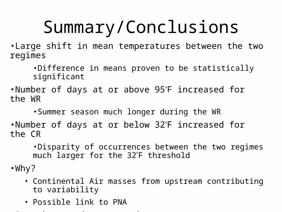
Summary/Conclusions•Large shift in mean temperatures between the two regimes

•Difference in means proven to be statistically significant

•Number of days at or above 95F increased for the WR

•Summer season much longer during the WR

•Number of days at or below 32F increased for the CR

•Disparity of occurrences between the two regimes much larger for the 32F threshold

•Why?

• Continental Air masses from upstream contributing to variability

• Possible link to PNA

•Questions to be answered

• What are the causes for this multi-decadal shift in temperatures and is the signal present in other regions of the U.S.

Acknowledgements

Melissa Griffin David Zierden

Mark Bourassa, Eric Chassignet, Philip Sura, Meredith Field, Dmitry Dukhovskoy, Preston Leftwich, J.J. O’Brien, Precious Lewis

I would like to thank the following people for their contributions

Questions?

PNA pattern• The positive phase of the PNA pattern is

associated with below-average temperatures across the south-central and southeastern U.S.

• PNA pattern has strong ties to ENSO– Positive PNA is associated with El Niño– Negative PNA is associated with La Niña

Lathers and Palecki(1991)

PNA pattern

Spatial Correlation