characterizing distributions of surface ozone and its impact on grain production in china, japan and...

Atmospheric Environment 38 (2004) 4383–4402

ARTICLE IN PRESS

AE International – Asia

*Correspond

E-mail addr

1352-2310/$ - se

doi:10.1016/j.at

Characterizing distributions of surface ozone and its impacton grain production in China, Japan and South Korea:

1990 and 2020

Xiaoping Wang, Denise L. Mauzerall*

Science, Technology and Environmental Policy Program, Woodrow Wilson School of Public and International Affairs,

Princeton University, Princeton, NJ 08544, USA

Received 9 November 2003; accepted 10 March 2004

Abstract

Using an integrated assessment approach, we evaluate the impact that surface O3 in East Asia had on agricultural

production in 1990 and is projected to have in 2020. We also examine the effect that emission controls and the

enforcement of environmental standards could have in increasing grain production in China. We find that given

projected increases in O3 concentrations in the region, East Asian countries are presently on the cusp of substantial

reductions in grain production. Our conservative estimates, based on 7- and 12-h mean (M7 or M12) exposure indices,

show that due to O3 concentrations in 1990 China, Japan and South Korea lost 1–9% of their yield of wheat, rice and

corn and 23–27% of their yield of soybeans, with an associated value of 1990US$ 3.5, 1.2 and 0.24 billion, respectively.

In 2020, assuming no change in agricultural production practices and again using M7 and M12 exposure indices, grain

loss due to increased levels of O3 pollution is projected to increase to 2–16% for wheat, rice and corn and 28–35% for

soybeans; the associated economic costs are expected to increase by 82%, 33%, and 67% in 2020 over 1990 for China,

Japan and South Korea, respectively. For most crops, the yield losses in 1990 based on SUM06 or W126 exposure

indices are lower than yield losses estimated using M7 or M12 exposure indices in China and Japan but higher in South

Korea; in 2020, the yield losses based on SUM06 or W126 exposure indices are substantially higher for all crops in all

three countries. This is primarily due to the nature of the cumulative indices which weight elevated values of O3 more

heavily than lower values. Chinese compliance with its ambient O3 standard in 1990 would have had a limited effect in

reducing the grain yield loss caused by O3 exposure, resulting in only US$ 0.2 billion of additional grain revenues, but in

2020 compliance could reduce the yield loss by one third and lead to an increase of US$ 2.6 (M7 or M12) –27 (SUM06)

billion in grain revenues. We conclude that East Asian countries may have tremendous losses of crop yields in the near

future due to projected increases in O3 concentrations. They likely could achieve substantial increases in future

agricultural production through reduction of surface O3 concentrations and/or use of O3 resistant crop cultivars.

r 2004 Elsevier Ltd. All rights reserved.

Keywords: Air pollution impacts; Ozone; Agriculture; East Asia; Integrated assessment

ing author. Fax: +1-609-258-6082.

ess: [email protected] (D.L. Mauzerall).

e front matter r 2004 Elsevier Ltd. All rights reserve

mosenv.2004.03.067

1. Introduction

In this paper, we examine the impact of surface ozone

(O3) on grain production in East Asia for 1990 and 2020.

We also estimate the economic damage associated with

yield reductions, and examine the effectiveness of

d.

ARTICLE IN PRESSX. Wang, D.L. Mauzerall / Atmospheric Environment 38 (2004) 4383–44024384

possible pollution control policies in reducing the O3

impact on China’s grain production. The study includes

three countries: China, Japan and South Korea (Fig. 1),

with an emphasis on China.

East Asia is one of the most dynamic regions in the

world. It hosts 25% of the world’s population, consumes

19% of its total energy and produces 21% of its total

cereals (Food and Agricultural Organization, 2003;

International Energy Agency, 1999). Agriculture is an

important sector in the Chinese economy, accounting

for 27% of its total GDP in 1990, although its share has

been decreasing. China has 7% of the world’s arable

Fig. 1. The map shows the central point of the MOZART-2 grid cells

(black curves), and monitoring stations (stars and labeled station

Numbers on the maps are provincial indices for China with correspo

land yet feeds over 20% of the world’s population

(Wang et al., 1996).

Food security is a long-standing concern of China.

China has long stressed its food self-sufficiency policy

and rebutted the claim of its potential dependence on

food imports (Brown, 1995). However, this self-suffi-

ciency policy has been relaxed over the last decade as

China negotiated to join the World Trade Organization

(WTO). China became a net grain importer in 1999

(Chadha, 2000) and is expected to import about 10% of

its wheat in 2004 from the United States alone (Tuan

and Hsu, 2001). Despite the lower-priced imports, the

(dots), provincial boundaries of China, Japan and South Korea

names) where observations are compared with model results.

nding province names listed below.

ARTICLE IN PRESSX. Wang, D.L. Mauzerall / Atmospheric Environment 38 (2004) 4383–4402 4385

Chinese government aims to maintain 95% grain self

sufficiency to protect the livelihood of the two-thirds of

its population residing in the countryside (Chadha,

2000). In shaping China’s agricultural policy or the

prognosticative debate, little consideration has been

given to the potential impact of increasing air pollution

on agricultural production.

Due to population growth and increased fossil fuel

consumption, East Asia is experiencing serious air

pollution. Particulate concentrations are above the

average of most developed countries and the World

Health Organization (WHO) standard. Increasing nitro-

gen oxide (NOx=NO+NO2) emissions contribute to

acid deposition and are a primary precursor for O3 and

particulate formation. Emissions of major pollutants are

expected to increase substantially in the next 20 years

(Streets and Waldhoff, 2000). As a result, in this paper

we predict substantial increases in summer O3 levels by

2020. Trans-boundary air pollution has also become an

increasing concern for this region. Back-trajectory

analyses have suggested that anthropogenic emissions

in continental East Asia contribute significantly to O3

concentrations observed in Japan (Pochanart et al.,

2002, 2004). There is also evidence that outflow from the

Asian continent elevates pollutant levels over the Pacific

Ocean (Jacob et al., 2003; Mauzerall et al., 2000; Wild

and Akimoto, 2001), and reach as far as the west coast

of the United States (Jaffe et al., 2003).

Field experiments, notably the National Crop Loss

Assessment Network (NCLAN) experimental studies in

the US in the early 1980s and the European Open-Top

Chamber (EOTC) study in 1987–1991, found that

elevated surface O3 concentrations can substantially

reduce grain yield (EEA, 1999; EPA, 1996). Based on

the NCLAN results, the US EPA estimated that due to

ambient O3 concentrations, the yields of about one third

of US crops decreased by 10%. In some areas such as

California, the losses were likely higher (EPA, 1996).

Much of the European Union could be losing more than

5% of their crop yield due to exposure to O3 (Mauzerall

and Wang, 2001).

Few studies have been conducted in East Asia

examining the impact of air pollution on agriculture

(Ashmore and Marshall, 1999; Mauzerall and Wang,

2001). Measurements of O3 concentrations at five

locations in China suggest that impacts on Chinese

wheat may be sufficiently high to affect China’s crop

yield in the 1990s (Chameides et al., 1999; Li et al.,

1999). Field experiments conducted in the UK to

investigate the sensitivity of Chinese crops to typical

O3 levels in central China found that rice cultivars

grown in China may be more sensitive to O3 than

cultivars grown in Pakistan, Japan, and the US (Zheng

et al., 1998). Kobayashi et al. (1995) found that the

effect of O3 on rice yield reduction in Japan was

comparable to that reported for rice cultivars in

California. Using an integrated assessment approach

but a lower resolution atmospheric model than we use

(Aunan et al., 2000) estimated that reductions in crop

yields in 1990 in China were o3% for most crops

(except soybeans) but that crop losses for soybeans and

spring wheat might reach 20% and 30% by 2020.

Section 2 of this paper describes the integrated

assessment approach we use which includes atmospheric

modeling, assessment of crop yield reduction due to O3

exposure and economic valuation of the grain yield lost.

Section 3 presents our analysis of the impact of surface

O3 concentrations on grain yields for 1990 and 2020,

including O3 distributions, crop exposures, crop produc-

tion losses and the associated economic costs. It also

shows the effect that compliance with the current

Chinese O3 standard would have on improving grain

yields for the two case years. In Section 4, we discuss the

uncertainty and limitations of this undertaking and

policy implications. Section 5 is a summary.

2. Methodology

2.1. Distribution of selected grain crops in East Asia

Four major grain crops are selected in this study for

China and South Korea: rice, wheat, corn and soybeans.

Only rice, wheat and soybeans are included in the

analysis of Japanese yield losses because corn is a minor

crop in Japan. In 1990, these crops accounted for 82%,

92% and 87% of the total sown area for grain

production, and 63%, 46% and 61% of the total area

sown for agricultural production in China, Japan and

South Korea, respectively (China State Statistics Ad-

ministration, 1992; Japan Statistical Bureau, 1992; The

Korean Statistical Association, 1991). In China, most of

the four crops are grown in the eastern part of the

country (see http://www.iiasa.ac.at/Research/LUC/Chi-

naFood/data/maps/crops/all m.htm for details). Rice

and soybeans in Japan and South Korea and corn in

South Korea are evenly distributed within each country.

Wheat in Japan is grown primarily in Hokkaido, the

most northern province. Wheat is a minor crop in South

Korea which is primarily grown in the eastern part of

the country.

Due to the heterogeneous climate throughout China,

some crops are grown more than once a year in some

provinces. As ambient O3 levels have strong diurnal and

seasonal cycles, the same crops grown in different

seasons experience different O3 exposure and resulting

yield reductions. Thus we conduct separate analyses for

the following crops: winter wheat, spring wheat, single-

cropping rice, double-cropping early rice, double-crop-

ping late rice, as well as spring and summer corn. Some

areas of China grow three-cropping rice, but we do not

include this category because the practice is limited. All

http://www.iiasa.ac.at/Research/LUC/ChinaFood/data/maps/crops/all_m.htm



ARTICLE IN PRESS

Table 2

2020/1990 Scaling factors derived from the IPCC B2-Message

scenario for reactive pollutants

Asiaa ALMb OECD90c REFd

NOx 2.516 1.392 1.25 0.927

CO 1.527 1.170 1.101 1.06

VOCs 1.575 1.365 1.064 1.153

a ‘Asia’ represents all developing countries in Asia, excluding

the Middle East.b ‘ALM’ represents all developing countries in Africa, Latin

America and the Middle East.c ‘OECD’ groups together all member countries of the

Organization for Economic Cooperation and Development as

of 1990 which include the US, Canada, western Europe, Japan

and Australia.d ‘REF’ represents countries undergoing economic reform

and groups together the eastern European countries and the

newly independent states of the former Soviet Union.

X. Wang, D.L. Mauzerall / Atmospheric Environment 38 (2004) 4383–44024386

crops are grown once a year in South Korea and Japan.

Based on the growing seasons, wheat, rice and corn in

South Korea and Japan generally correspond to winter

wheat, single rice and summer corn in China.

2.2. Integrated assessment

In this analysis, we use an integrated approach that

incorporates atmospheric modeling, plant exposure–

yield response studies and economic assessment to

estimate the value of the yields lost due to O3 exposure.

A similar approach has been used to evaluate reductions

in agricultural yields caused by anthropogenic air

pollution in the United States (Adams et al., 1989) and

in China (Aunan et al., 2000). The steps for our

approach are explained in Table 1.

2.2.1. MOZART-2 model simulation

We use MOZART-2 (Model of Ozone and Related

Chemical Tracers, Version 2) to simulate ambient O3

concentrations for 1990 and 2020. The model is fully

described and evaluated in Horowitz et al. (2003).

MOZART-2 contains a detailed representation of

tropospheric ozone-nitrogen oxide-hydrocarbon chem-

istry, accounts for surface emissions and emissions from

lightning and aircraft, advective and convective trans-

port, boundary layer exchange, and wet and dry

deposition. It simulates the concentration distributions

of 63 chemical species. The model has a horizontal

resolution of 2.8� latitude� 2.8� longitude and includes

34 hybrid vertical levels extending from the surface to

approximately 40 km. The model runs at a time step of

20min for all processes, and is driven by meteorological

inputs from the Middle Atmosphere Community Cli-

mate Model Version 3 (MACCM3), a general circula-

tion model.

Surface emissions used in MOZART-2 include those

from fossil fuel combustion, biomass burning, biogenic

emissions from vegetation and soils, and oceanic

emissions. The 1990 anthropogenic emissions are based

on the EDGAR v2.0 inventory (Olivier et al., 1996) with

modifications. Biomass burning and biogenic emissions

are also included and are described in Horowitz et al.

Table 1

Structure of integrated assessment

Intermediate outcome Method

(1) Surface O3 concentrations Simulated using the 3-D global

(2) Plant exposures to O3 Calculated M7, M12, SUM06 an

(3) Yield loss Estimated for 1990 and 2020 ba

NCLAN study

(4) Economic values Estimated value of lost grain yie

(5) Policy implications Estimated the potential yield gai

1990 and/or 2020

(2003). 2020 emissions are obtained by scaling the

spatially and temporally varying global 1990 anthro-

pogenic emissions by the ratio of 2020/1990 total

regional emissions specified in the Intergovernmental

Panel on Climate Change (IPCC) B2-Message scenario

(IPCC, 2000). The emission scaling factors are listed in

Table 2. The IPCC-B2-Message scenario was chosen to

represent a world in which there is moderate population

growth, intermediate levels of economic development,

increased concern for environmental and social sustain-

ability, and less rapid technological development than in

the A1 and B1 storylines. Projections of global anthro-

pogenic emissions of reactive trace gases in 2020 range

from highest to lowest from A2, to A1, B2 and finally B1

marker storylines (IPCC, 2000). Hence, the simulation

conducted here using the B2 storyline is using global

emissions that are substantially lower than a ‘worst case’

scenario for most species. One exception is that NOx

emissions from Asia in the B2 storyline are higher than

in the A2 storyline. However, the resulting Asian NOx

scaling factor of 2.5 is supported by Streets and

Waldhoff (2000). The 2020 methane concentrations

and emissions used in MOZART-2 are scaled globally

by the 2020-to-1990 ratio of 1.117 (IPCC, 2000).

chemical tracer model MOZART-2 for 1990 and 2020

d W126 (see Section 2.2.3 below for their definitions)

sed on exposure—response functions obtained from the US

ld based on the producer prices for 1990

ns if current ambient air quality standards for O3 were met in


The simulated 1990 global distributions of O3 and its

precursors were evaluated extensively by comparison

with observational data (Horowitz et al., 2003). The

simulated seasonality, horizontal and vertical gradients

of O3 above the surface are generally in good agreement

with observations. In Section 3, we compare simulated

O3 concentrations with surface observations from 6

stations in China, Japan and South Korea, which were

not included in Horowitz et al. (2003).

For the agricultural impact analysis, we use hourly O3

concentrations from the bottom layer of the model

(extending from the surface to approximately 120m). As

agricultural data is usually available by administrative

regions—in our case, by province, we convert O3

concentrations within grid cells to concentrations within

provinces. The provincial boundaries often partially

overlap one or more MOZART-2 grid cells (Fig. 1). To

capture this feature, we divide each MOZART-2 grid

cell evenly into 36 smaller ones, each with the same O3

concentration as the original grid, and then average the

concentrations of all the smaller cells that fall into a

province to obtain a provincial concentration.

2.2.2. Plant exposure

No large-scale field experiments have been conducted

in Asia to investigate plant exposure to O3 and the

subsequent exposure–yield loss relationship for crops.

As mentioned in the introduction, two comprehensive,

large-scale field studies have been carried out in Europe

and in the US. The EOTC studies conducted in Europe

mainly focused on wheat, but the US NCLAN studies

included, among others, wheat, corn and soybeans that

are also of interest to this study. Therefore, we use

exposure indices and corresponding exposure–response

relationships obtained in the US NCLAN studies for

wheat, corn and soybeans. Rice is not a major crop in

the US or Europe, and was not included in the NCLAN

or EOTC studies. Kats et al. (1985) carried out an

independent regional rice study in the San Joaquin

Valley of California exploring the impact of O3 on rice

yields. Adams et al. (1989) fitted the experimental data

obtained under this study with a Weibull function and

derived a M7-based exposure–yield relationship for rice.

Individual field studies for rice have also been carried

out in Japan (Kobayashi et al., 1995) and Pakistan

(Kobayashi et al., 1995; Wahid et al., 1995a,b). Rice

yield loss due to O3 exposure in Japan was found to be

similar to that in the US, but in Pakistan it was higher.

We choose to use the Adams et al. (1989) result for rice

in our analysis as a conservative estimate.

Four exposure indices have been used most in the US

NCLAN studies. During the NCLAN field experiments,

7-h (900–1559 hours) seasonal mean O3 concentrations

(M7) were initially used to characterize crop exposure,

and at a later stage 12-h (800–1959 hours) seasonal

means (M12) were introduced in order to include more

of the elevated O3 concentrations (Hogsett et al., 1988).

However, in the post-experimental data analysis, cumu-

lative indices (e.g. SUM06 and W126) were found to be

a better fit to the yield loss data (EPA, 1996; Mauzerall

and Wang, 2001; Tingey et al., 1991). SUM06 empha-

sizes both exposure duration and peak O3 concentra-

tions. It is defined as:

SUM06 ðppmhÞ ¼Xn

i¼1

½CO3�i for CO3

X0:06 ppm; ð1Þ

where CO3is the hourly mean O3 concentration (ppm), i

is the index and n is the total number of hours in three

consecutive months of a growing season for which the

SUM06 value is highest. The definition of W126 is

similar to that of SUM06 except that it does not rely on

a threshold value. Rather, it gives lower weight to lower

concentrations and higher weight to higher concentra-

tions based on a weighting function. The weighting

factor wi for the ith hour is defined as:

wi ¼ 1=f1þ 4403 exp½0:126 ðCO3Þi�g: ð2Þ

The general form of W126 is:

W126 ðppmÞ ¼Xn

i¼1

wi ½CO3�i: ð3Þ

While the current knowledge of the physiology of

plant response to O3 exposure is not sufficient to fully

explain the difference in the yield responses obtained

with different indices, the use of cumulative O3 exposure

indices is favored by most experts (e.g. Lee and Hogsett,

1999; Lefohn and Foley, 1992; Lefohn et al., 1989;

Tingey et al., 1991). Europe has adopted a cumulative

exposure index, AOT40, for its ambient O3 standard

(EEA, 1999). (AOT40 is defined as the sum of the

difference between hourly O3 concentrations above

40 ppb during daylight hours when clear sky radiation

is above 50Wm2 for 3 months —usually May–July.)

However, the ambient O3 standards in the US and East

Asia are still based on 8-h average or 1-h maximum

concentrations. To illustrate the range of uncertainty of

the results associated with the use of different exposure

indices, we include both the mean and cumulative

exposure indices in our analysis.

The growing season typically spans from planting to

ripening and is species and location dependent. How-

ever, until emerging from the ground, the plant is

thought to be unaffected by O3. Hence in our analysis

the growing season is defined by an emerging date (a

transplanting date for rice) and a ripening date, and

varies by crop and province (Fig. 2). For the study

region, O3 measurements and model simulations in-

dicate that O3 levels appear to peak in the spring,

decrease in the summer and then increase in the fall

(Ghim and Chang, 2000; Mauzerall et al., 2000; Wang

et al., 2001). Since higher O3 levels usually occur in the

late stage of the growing season (spring for wheat and

ARTICLE IN PRESS

Julian Day

Soybean Ripening

Rice Ripening

Corn Planting

Rice Transplanting

Winter Wheat Ripening

Winter Wheat Planting

Corn Ripening

Soybean Planting

0 15 30 45 60 75 90 105 120 135 150 165 180 195 210 225 240 255 270 285 300 315 330 345 360

+ China KoreaLegend: Japan

Fig. 2. Growing seasons for crops grown in China, Japan and Korea. The data points in a line correspond to the planting or ripening

dates in individual provinces in each country. For a cluster of three lines, from top to bottom, are China, Japan and South Korea; for a

cluster of two lines, the top line is for China, and the bottom line is for South Korea.


fall for rice, corn and soybeans), we expect the highest

three consecutive months for SUM06 and W126 to

mostly occur during the last 3 months of a crops

growing season, and consequently calculate SUM06 and

W126 during those periods. The growing season dates

were obtained from Gui and Liu (1984) for China, from

Kobayashi (2001) for Japan and from Ryou (2001) for

South Korea.

2.2.3. Yield loss

The Weibull function is widely used to express the

relationship between O3 exposure and crop yield

reduction. Its general form is (Lesser et al., 1990):

Y ¼ A exp½ðX=BÞC �; ð4Þ

where Y is the estimated mean yield, X the O3 exposure

index (M7, M12, SUM06 or W126 here), A the

theoretical yield at zero O3 concentration, B the scale

parameter for O3 exposure which reflects the dose at

which the expected response is reduced to 0.37A, and C

the shape parameter affecting the change in the

predicted rate of loss.

Relative yield losses (RYL) are defined as:

RYL ¼ 1 Y=Ybase; ð5Þ

where Ybase is the estimated mean yield at the reference

exposure index. We rely on the original sources of the

exposure–response functions for the reference levels for

different indices. The reference level is 25 ppb for M7,

20 ppb for M12, and 0 ppmh for SUM06 and 0 ppm for

W126 (EPA, 1996).

Because the response of crop yield to O3 exposure in

the NCLAN study varied by cultivar and experimental

location Lesser et al. (1990) used a regression model to

combine all field experimental data for different

cultivars of a crop in order to characterize the average

response of the crop to O3 concentrations. Weibull

functions based on 7- or 12-h seasonal means were then

derived for winter wheat, corn and soybeans; we use

these functions in our analysis. No single Weibull

function based on SUM06 or W126 has been developed

for an entire crop. Individual SUM06 and W126

exposure–response functions were fit for each crop

cultivar included in each of the 54 NCLAN case studies

(EPA, 1996). For the same crop, the Weibull parameters

A, B and C were found to differ across experimental

sites, up to an order of magnitude for soybeans. We

plotted all of the exposure–response functions from

individual case studies and found that the function with

median Weibull parameter values best represents the

characteristic exposure–response function for a given

crop species. Hence, we use median Weibull parameter

values to calculate SUM06 and W126 for each crop

category in our analysis.

Exposure–response functions used in this analysis are

shown in Table 3 and graphed in Fig. 3. At a given M7

or M12 value, the RYL is largest for soybeans, and least

for spring wheat and rice, with corn and winter wheat in

the middle. However, at a given SUM06/W126 value,

the RYL is largest for wheat, followed by soybeans and

corn. The ordering of RYL for the four crops when the

seasonal mean indices are used differs from the ordering

with the cumulative indices. This suggests that some

crops (e.g. soybeans) are more sensitive to long-term

exposure to modest O3 levels (characterized by seasonal

means) than frequent exposure to high O3 levels (which

are best captured by cumulative indices). Different

ordering could also be due to the different statistical

ARTICLE IN PRESS

Table 3

O3 exposure–yield response equations for rice, wheat, corn and soybeans based on 7-h and 12-h means, SUM06 and W126 indices

Crop Exposure–relative yield (RY) relationship Reference

Rice RY=exp [(M7/202)2.47]/exp [(25/202)2.47] Adams et al. (1989)

Wheat RY=exp [(M7/137)2.34]/exp [(25/137)2.34] (Winter wheat) Lesser et al. (1990)

RY=exp [(M7/186)3.2]/exp [(25/186)3.2] (Spring wheat) Adams et al. (1989)

RY=exp [(SUM06/52.32)2.176] Adapted from EPA (1996)a

RY=exp [(W126/51.2)1.747] Adapted from EPA (1996)a

Corn RY=exp [(M12/124)2.83]/exp [(20/124)2.83] Lesser et al. (1990)



Soybean RY=exp [(M12/107)1.58]/exp [(20/107)1.58] Lesser et al. (1990)



aWeibull parameters are given for each studied cultivars of a particular crop under NCLAN. We construct a single exposure–

response function for a crop by using the median Weibull parameters of all studied cultivars.

Fig. 3. O3 exposure–yield response functions used in this analysis for (a) 7-h (M7) or 12-h. (M12) seasonal O3 means, and cumulative

indices (b) SUM06, and (c) W126. The equations for these functions are shown in Table 3.

X. Wang, D.L. Mauzerall / Atmospheric Environment 38 (2004) 4383–4402 4389

methods used to derive the average exposure–response

function for individual crops. In addition, at high O3

concentrations, the cumulative indices predict larger

losses than do the mean indices. This is due largely to the

fact that higher concentrations are weighted much more

heavily with the cumulative than with the mean indices.

For example, for SUM06, O3 concentrations of 59 ppb

would be counted as zero (and hence would not result in

ARTICLE IN PRESS

Table 4

Producer prices of grains in 1990 (Food and Agricultural Organization, 2003)

China Japan South Korea

Yuan ton1 US$ ton1 yen ton1 US$ ton1 won ton1 US$ ton1

Wheat 636 133 161,733 1117 354,000 500

Rice 708 148 334,333 2309 817,254 1155

Corn 479 100 261,900 370

Soybeans 1073 224 241,667 1669 917,825 1297


a yield reduction) while concentrations of 62 ppb would

be counted as 2 ppbh for each hour the concentration

was 2 ppb above 60 ppb. With the mean indices,

concentrations that differ by only 3 ppb would result

in very similar estimates of yield losses.

Crop production loss (CPL) is calculated based on

RYL and actual output, that is:

CPL ¼RYL

1-RYL�Output; ð6Þ

where output means the actual annual yield of each crop

in 1990 and is obtained from the country statistical

yearbooks (China State Statistics Administration, 1992;

Japan Statistical Bureau, 1992; The Korean Statistical

Association, 1991). The national average RYL for each

crop is calculated as:

National Average RYL ¼Pn

i¼1½CPL�iPni¼1ð½CPL�i þ ½Output�iÞ

;

ð7Þ

where n is the number of provinces included for each

country (30 for China, 47 for Japan and 15 for South

Korea).

2.2.4. Economic analysis

We translate the crop production loss into economic

costs (EC) based on the commodity price, i.e. economic

costs=market price� crop production loss. This simple

revenue approach for economic analysis takes the

market price as given and ignores the feedback of

reduced grain output on the price, planting acreage, or

farmers’ input decisions. Westenbarger and Frisvold

(1995) reviewed several studies involving use of a general

equilibrium model with factor feedbacks and found that

the benefit measures derived from such a revenue

approach are within 20% of those derived from a

general equilibrium model. Due to lack of information

on domestic market prices in 1990 for the three

countries, we use the producer prices as surrogates for

market prices. The producer prices for different grains in

the three countries are presented in Table 4 (Food and

Agricultural Organization, 2003).

2.3. The effect of compliance

Ambient air quality standards in China include three

classes of standards that apply to different functional

zones. The Class I standard for O3 is an hourly average

concentration of 0.12mgm3 (56 ppb) not to be

exceeded at any hour in nature reserves, scenic sites

and protected areas; the Class II standard is an hourly

average of 0.16mgm3 (75 ppb) not to be exceeded at

any hour in designated residential, commercial, cultural,

general industrial and rural areas; the Class III O3

standard is an hourly average of 0.20mgm3 (93 ppb)

not to be exceeded at any hour in special industrial areas

(State Environmental Protection Agency of China,

1996). We examine the possible gain in crop yield that

would be achieved if the Class II standard were met

throughout China by substituting all the hourly

provincial averages above 75 with 75 ppb, and then

calculating the potential yield loss. The potential gain in

grain yield is calculated as the difference between yields

achieved with assumed compliance and the actual yield

loss. As we neglect the downward shift in all O3

concentrations that would occur if compliance with the

standard were actually achieved, we potentially under-

estimate the benefits of compliance.

3. Results

In this section, we first compare 1990 model

calculated O3 concentrations with the limited observa-

tions of O3 concentrations available in China, Japan and

South Korea. We then present model-simulated O3

distributions, crop exposures to O3, yield losses as well

as the resulting economic damage in East Asia for 1990

and 2020. Finally, we examine the effect on grain

production if China had attained its Class II O3

standard in 1990 and 2020.

3.1. Comparison of modeling results with surface

observations

We compare simulated monthly averages of O3

concentrations with surface observations available for

ARTICLE IN PRESS

Fig. 4. Comparison of observed (closed diamonds) and simulated (open squares) monthly mean 12-h daily average (8 a.m.–8 p.m.) O3

concentrations (ppb) in Lin’an (30�250N, 119�440E, 132m), Oki (36�170N, 133�110E, 90m), Happo (36�410N, 137�480E, 1840m), and

three Korean sites—k1 (37�250N, 126�100E), k2 (33�90N, 126�70E), and k3 (36�260N, 126�50E). The observations for Lin’an were made

from August 1999 to July 2000 (Wang et al., 2001). The measurements for Happo and Oki were made continuously in 1996 and 1997

(Mauzerall et al., 2000). The observations at the three Korean sites were made in 2001 and 2002 (Kim, 2003). Monthly averages based

on the 2-years of observations in Japan and Korea are used for comparison.


six stations in this region (see Fig. 1 for station

locations); results are shown in Fig. 4. MOZART-2

generally reproduces O3 concentrations reasonably

well at all six sites. At Lin’an and at the third Korean

site (k3), the model over predicts the O3 concentrations

for all but 1 month by several to 20 ppb. At the

other four sites, the model tends to overestimate O3

concentrations in the fall months. The over-estimate in

model calculated autumn O3 concentrations will

result in an over-estimate of O3 impacts on yields,

particularly for soybeans that are harvested in late

autumn. Other than the model weaknesses discussed in

Horowitz et al. (2003), these discrepancies could

result from the fact that the climatological winds

used in MOZART-2 are likely to be different from the

conditions prevailing during the measurement

periods and that emissions from biomass burning in

the model may be overestimated at high northern

latitudes in autumn and hence contribute excess O3

precursors.

3.2. Distribution of O3 concentrations and crop exposures

Monthly means of daily 12-h average O3 concentra-

tions simulated by MOZART-2 for 1990, 2020

and the difference between 1990 and 2020 for

East Asia are shown in Fig. 5 for April, July and

October. While O3 concentrations are projected to

increase substantially in July for all three countries in

2020 over 1990, the increase is largest in China

and smallest in Japan. In July 2020, surface O3

concentrations in central China are predicted to

exceed 65 ppb, an average increase of approximately

15 ppb over 1990 levels. Average concentrations in

Japan and South Korea are predicted to be o60 ppb

in July 2020 with an increase of approximately 5 ppb

from 1990 levels. Increases in O3 concentrations

in April and October are predicted to largely be in

southern China and southeast Asia with decreases

predicted for north-eastern China and Korea. These

decreases occur where NOx emissions are largest

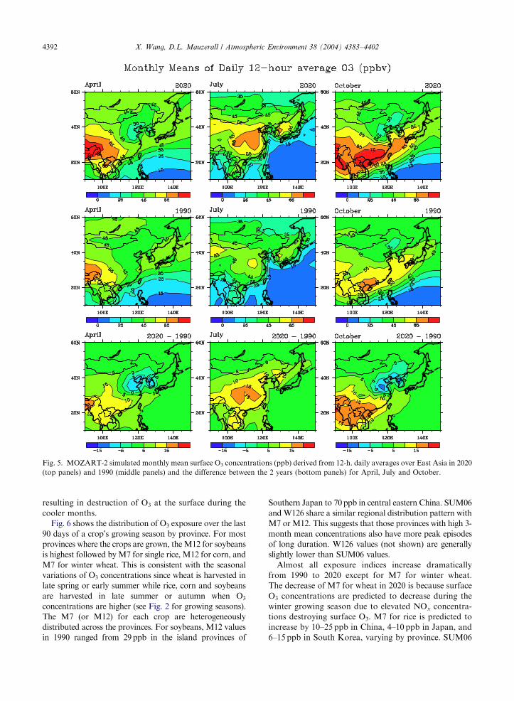
ARTICLE IN PRESS

Fig. 5. MOZART-2 simulated monthly mean surface O3 concentrations (ppb) derived from 12-h. daily averages over East Asia in 2020

(top panels) and 1990 (middle panels) and the difference between the 2 years (bottom panels) for April, July and October.


resulting in destruction of O3 at the surface during the

cooler months.

Fig. 6 shows the distribution of O3 exposure over the last

90 days of a crop’s growing season by province. For most

provinces where the crops are grown, theM12 for soybeans

is highest followed byM7 for single rice, M12 for corn, and

M7 for winter wheat. This is consistent with the seasonal

variations of O3 concentrations since wheat is harvested in

late spring or early summer while rice, corn and soybeans

are harvested in late summer or autumn when O3

concentrations are higher (see Fig. 2 for growing seasons).

The M7 (or M12) for each crop are heterogeneously

distributed across the provinces. For soybeans, M12 values

in 1990 ranged from 29ppb in the island provinces of

Southern Japan to 70ppb in central eastern China. SUM06

and W126 share a similar regional distribution pattern with

M7 or M12. This suggests that those provinces with high 3-

month mean concentrations also have more peak episodes

of long duration. W126 values (not shown) are generally

slightly lower than SUM06 values.

Almost all exposure indices increase dramatically

from 1990 to 2020 except for M7 for winter wheat.

The decrease of M7 for wheat in 2020 is because surface

O3 concentrations are predicted to decrease during the

winter growing season due to elevated NOx concentra-

tions destroying surface O3. M7 for rice is predicted to

increase by 10–25 ppb in China, 4–10 ppb in Japan, and

6–15 ppb in South Korea, varying by province. SUM06


for soybeans increases by 6–70 ppmh in China, 8–

32 ppmh in Japan, and 19–39 ppmh in Korea with

variation occurring among provinces.

3.3. Relative yield loss

Calculated national average yield losses for China,

South Korea and Japan in 1990 and 2020 are shown in

Fig. 6. Distributions of crop exposure and RYL by province an

concentrations over specific crop growing seasons, (b) shows the SUM

the relative yield loss (RYL) resulting from these exposures.

Table 5. The O3-induced RYL in 1990 was highest in

South Korea and was comparable for China and Japan.

The SUM06 and W126 RYLs in 1990 for winter wheat

in Korea reached 43% and 39%, respectively. However,

winter wheat is a minor crop in Korea, and thus the

economic consequence is limited. The M7/M12 RYL for

soybeans was as high as 23% in China and Japan and

27% in South Korea in 1990. The curvature of the

d crop in 1990 and 2020. (a) Shows 7- and 12-h mean O3

06 O3 exposure for specific crop growing seasons, and (c) shows

ARTICLE IN PRESS

Fig. 6 (continued).


dose–response functions and O3 concentrations during

different growing seasons are the two factors that

determine the differences in RYL between crops. Both

factors contribute to soybeans having a very high RYL. As

shown in Fig. 2, the last 3 months of the growing season

for soybeans are usually from mid-August to mid-

November when seasonal O3 concentrations are highest.

While the three countries have similar RYL in 1990

for rice, the RYLs for wheat and soybeans in South

Korea are much higher than in China and Japan. As we

use the same dose–response functions for all three

countries, exposure, determined by growing season

periods and O3 concentrations, is the only factor

determining the inter- and intra-country variations in

RYL for the same crop. Higher O3 concentrations

during the growing season in major agricultural

production areas (particularly for soybeans) in the south

of South Korea contribute to higher RYL nationwide.

We project that the RYL in 2020 will increase

tremendously in all three countries for all crops with

the increase more than doubling in China, being

moderate in South Korea and modest in Japan. Using

the SUM06 metric, we project enormous reductions in

yields of winter wheat (63%), summer corn (64%) and

soybeans (45% ) in China and similar reductions of 50–

60% of these crops in South Korea. Using the mean

indices, RYLs are smaller and range between 7 and

35%. The cumulative index-based RYLs project larger

yield reductions in 2020 than the seasonal mean RYLs

because as O3 concentrations increase, the cumulative

indices, which give greater weight to higher concentra-

tions and lower or zero weight to lower concentrations,

ARTICLE IN PRESS

Fig. 6 (continued).


increase much faster than M7 or M12 which give equal

weight to all concentrations.

3.4. Crop production loss and economic damage

Table 6 shows calculated crop production losses due

to O3 exposure and the associated economic costs in

1990 for each crop and country under consideration.

Based on M7/M12 indices, the crop production

losses of the four grain crops in China, Japan and

South Korea in 1990 were 25, 0.6 and 0.2 million

metric tons, respectively. The associated economic

costs (EC) were approximately 3.5, 1.2 and 0.24 billon

US dollars respectively given the producer prices of

grain in each country in 1990 (Food and Agricultural

Organization, 2003). Cross-comparison of the total

economic costs based on M7/M12, SUM06 and W126

cannot be made due to lack of SUM06 or W126 data

for rice.

As it is difficult to predict the actual yields and grain

prices in 2020, we calculate the CPL and EC for 2020 by

making a simple and conservative assumption that the

ARTICLE IN PRESS

Table 5

O3-induced relative yield loss (%) for East Asia

1990 2020

M7/M12 SUM06 W126 M7/M12 SUM06 W126

China Winter wheat 6 13 12 7 63 41

Spring wheat 0.8 0.5 3 2 30 22

Single rice 4 8

Double E rice 3 7

Double L rice 5 10

Spring corn 8 3.5 1 16 39 24

Summer corn 8 9.2 4 16 64 45

Soybeans 23 19 15 33 45 37

Japan Winter wheat 7 5 6 8.7 16 14

Single rice 4 5.3

Soybeans 24 18 15 28 32 25

South Korea Winter wheat 8.8 43 39 8 59 47

Single rice 2 4

Corn 3 18 4 4 50 27

Soybeans 27 36 26 35 59 47

Table 6

O3-induced crop production loss (CPL) and associated economic cost (EC) in 1990

Actual grain output M7/M12 SUM06 W126

CPL EC CPL EC CPL EC

China

Wheat 99,356 5,523 735 12,738 1694 12,584 1674

Rice 191,748 8,018 1187

Corn 96,819 8,237 824 6,636 664 2,745 275

Soybeans 11,000 3,225 722 2,603 583 1,960 439

Subtotal 25,002 3467

Japan

Wheat 913 63 70 50 56 58 65

Rice 10,356 419 967

Soybeans 254 78 130 54 90 44 73

Subtotal 560 1168

Korea

Wheat 1 0 0 1 0.5 1 0.5

Rice 5,606 112 129

Corn 120 4 1 26 10 5 2

Soybeans 233 85 110 130 169 83 108

Subtotal 200 241

Notes: 1. The unit for actual yields and CPL is kton yr1, and for EC is million 1990 US dollars.

2. Actual yields are obtained from the country statistical yearbooks (China State Statistics Administration, 1992; Japan Statistical

Bureau, 1992; The Korean Statistical Association, 1991).


actual yields and grain prices in 2020 are the same as in

1990. The grain yields in China have in fact constantly

increased over the last two decades thanks to the

introduction of increasingly productive varieties, im-

plementation of a rural household responsibility system

and the increasing use of fertilizer. However, growth

rates have slowed in recent years due to diminishing

returns from increased fertilizer use and agricultural

ARTICLE IN PRESS

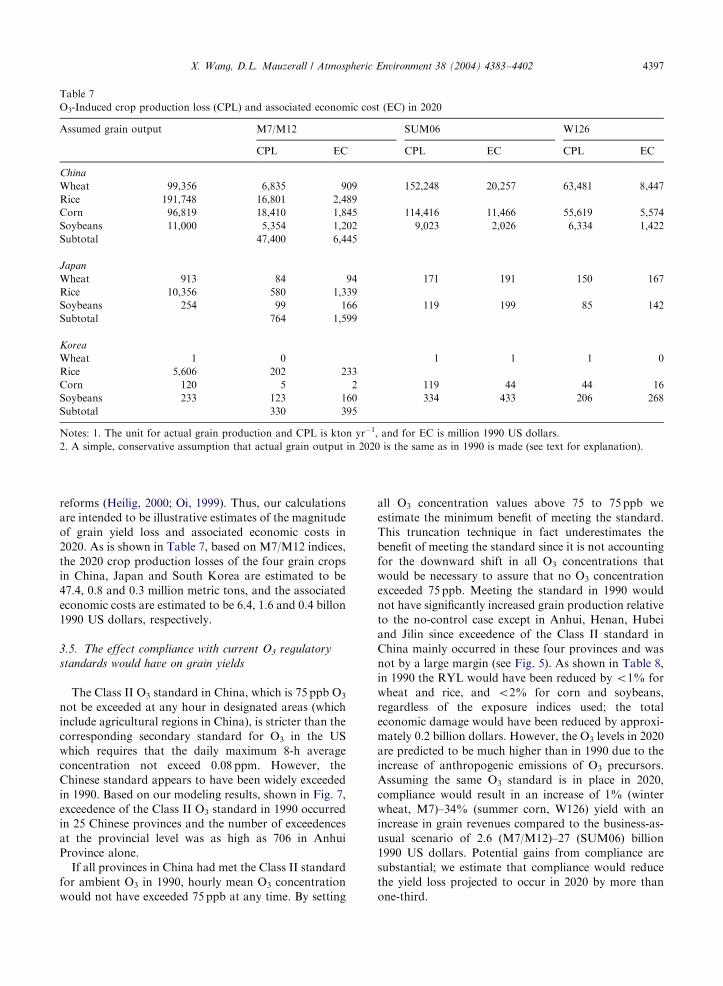
Table 7

O3-Induced crop production loss (CPL) and associated economic cost (EC) in 2020

Assumed grain output M7/M12 SUM06 W126

CPL EC CPL EC CPL EC

China

Wheat 99,356 6,835 909 152,248 20,257 63,481 8,447

Rice 191,748 16,801 2,489

Corn 96,819 18,410 1,845 114,416 11,466 55,619 5,574

Soybeans 11,000 5,354 1,202 9,023 2,026 6,334 1,422

Subtotal 47,400 6,445

Japan

Wheat 913 84 94 171 191 150 167

Rice 10,356 580 1,339

Soybeans 254 99 166 119 199 85 142

Subtotal 764 1,599

Korea

Wheat 1 0 1 1 1 0

Rice 5,606 202 233

Corn 120 5 2 119 44 44 16

Soybeans 233 123 160 334 433 206 268

Subtotal 330 395

Notes: 1. The unit for actual grain production and CPL is kton yr1, and for EC is million 1990 US dollars.

2. A simple, conservative assumption that actual grain output in 2020 is the same as in 1990 is made (see text for explanation).


reforms (Heilig, 2000; Oi, 1999). Thus, our calculations

are intended to be illustrative estimates of the magnitude

of grain yield loss and associated economic costs in

2020. As is shown in Table 7, based on M7/M12 indices,

the 2020 crop production losses of the four grain crops

in China, Japan and South Korea are estimated to be

47.4, 0.8 and 0.3 million metric tons, and the associated

economic costs are estimated to be 6.4, 1.6 and 0.4 billon

1990 US dollars, respectively.

3.5. The effect compliance with current O3 regulatory

standards would have on grain yields

The Class II O3 standard in China, which is 75 ppb O3

not be exceeded at any hour in designated areas (which

include agricultural regions in China), is stricter than the

corresponding secondary standard for O3 in the US

which requires that the daily maximum 8-h average

concentration not exceed 0.08 ppm. However, the

Chinese standard appears to have been widely exceeded

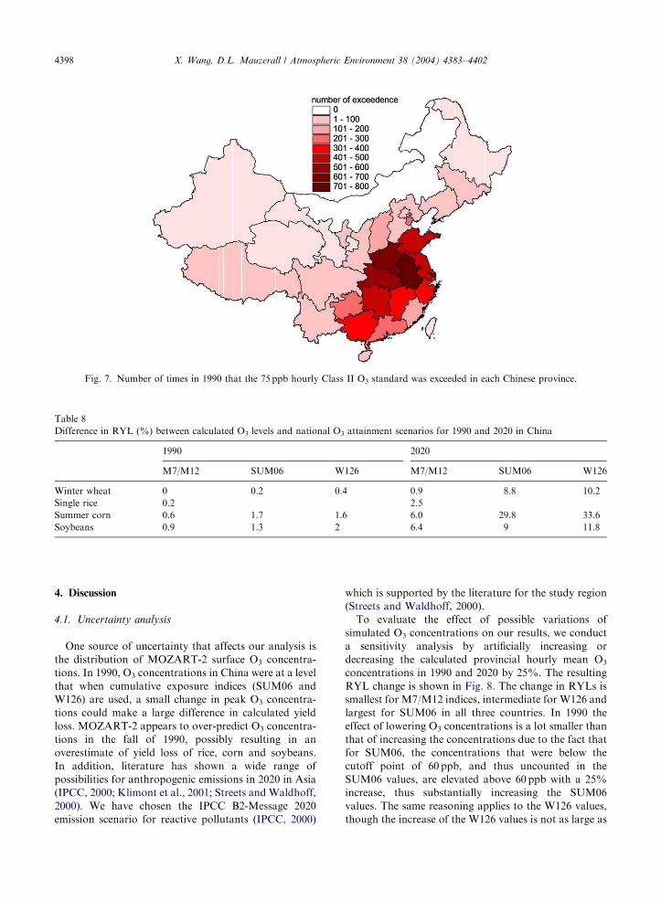
in 1990. Based on our modeling results, shown in Fig. 7,

exceedence of the Class II O3 standard in 1990 occurred

in 25 Chinese provinces and the number of exceedences

at the provincial level was as high as 706 in Anhui

Province alone.

If all provinces in China had met the Class II standard

for ambient O3 in 1990, hourly mean O3 concentration

would not have exceeded 75 ppb at any time. By setting

all O3 concentration values above 75 to 75 ppb we

estimate the minimum benefit of meeting the standard.

This truncation technique in fact underestimates the

benefit of meeting the standard since it is not accounting

for the downward shift in all O3 concentrations that

would be necessary to assure that no O3 concentration

exceeded 75 ppb. Meeting the standard in 1990 would

not have significantly increased grain production relative

to the no-control case except in Anhui, Henan, Hubei

and Jilin since exceedence of the Class II standard in

China mainly occurred in these four provinces and was

not by a large margin (see Fig. 5). As shown in Table 8,

in 1990 the RYL would have been reduced by o1% for

wheat and rice, and o2% for corn and soybeans,

regardless of the exposure indices used; the total

economic damage would have been reduced by approxi-

mately 0.2 billion dollars. However, the O3 levels in 2020

are predicted to be much higher than in 1990 due to the

increase of anthropogenic emissions of O3 precursors.

Assuming the same O3 standard is in place in 2020,

compliance would result in an increase of 1% (winter

wheat, M7)–34% (summer corn, W126) yield with an

increase in grain revenues compared to the business-as-

usual scenario of 2.6 (M7/M12)–27 (SUM06) billion

1990 US dollars. Potential gains from compliance are

substantial; we estimate that compliance would reduce

the yield loss projected to occur in 2020 by more than

one-third.

ARTICLE IN PRESS

Fig. 7. Number of times in 1990 that the 75 ppb hourly Class II O3 standard was exceeded in each Chinese province.

Table 8

Difference in RYL (%) between calculated O3 levels and national O3 attainment scenarios for 1990 and 2020 in China

1990 2020

M7/M12 SUM06 W126 M7/M12 SUM06 W126

Winter wheat 0 0.2 0.4 0.9 8.8 10.2

Single rice 0.2 2.5

Summer corn 0.6 1.7 1.6 6.0 29.8 33.6

Soybeans 0.9 1.3 2 6.4 9 11.8


4. Discussion

4.1. Uncertainty analysis

One source of uncertainty that affects our analysis is

the distribution of MOZART-2 surface O3 concentra-

tions. In 1990, O3 concentrations in China were at a level

that when cumulative exposure indices (SUM06 and

W126) are used, a small change in peak O3 concentra-

tions could make a large difference in calculated yield

loss. MOZART-2 appears to over-predict O3 concentra-

tions in the fall of 1990, possibly resulting in an

overestimate of yield loss of rice, corn and soybeans.

In addition, literature has shown a wide range of

possibilities for anthropogenic emissions in 2020 in Asia

(IPCC, 2000; Klimont et al., 2001; Streets and Waldhoff,

2000). We have chosen the IPCC B2-Message 2020

emission scenario for reactive pollutants (IPCC, 2000)

which is supported by the literature for the study region

(Streets and Waldhoff, 2000).

To evaluate the effect of possible variations of

simulated O3 concentrations on our results, we conduct

a sensitivity analysis by artificially increasing or

decreasing the calculated provincial hourly mean O3

concentrations in 1990 and 2020 by 25%. The resulting

RYL change is shown in Fig. 8. The change in RYLs is

smallest for M7/M12 indices, intermediate for W126 and

largest for SUM06 in all three countries. In 1990 the

effect of lowering O3 concentrations is a lot smaller than

that of increasing the concentrations due to the fact that

for SUM06, the concentrations that were below the

cutoff point of 60 ppb, and thus uncounted in the

SUM06 values, are elevated above 60 ppb with a 25%

increase, thus substantially increasing the SUM06

values. The same reasoning applies to the W126 values,

though the increase of the W126 values is not as large as

ARTICLE IN PRESS

Fig. 8. Sensitivity of the RYL to O3 concentrations in China, Japan and South Korea. The upper bounds, mid-points and lower

bounds of the vertical lines define the RYL that corresponds to increases of all O3 concentrations by 25%, no change in O3

concentrations, and decreases of all O3 concentrations by 25%, respectively. Abbreviations: M=M7 or M12, S=SUM06, W=W126,

Wheat1=Winter Wheat, Wheat2=Spring Wheat, Rice1=Single Rice, Rice2=Double Early Rice, Rice3=Double Late Rice,

Corn1=Spring Corn, Corn2=Summer Corn.


that of SUM06 because the weights on the W126 index

are gradually increased around 60 ppb. In contrast, in

2020 after the threshold O3 level of 60 ppb is exceeded

for most crops, the RYLs are more evenly responsive to

an increase or decrease in O3. A few species such as

wheat and corn in China, as well as wheat in South

Korea will experience 100% RYL if the O3 concentra-

tions are 25% above the simulated levels in 2020 based

on the existing exposure–yield response functions. A

caveat is that such high O3 concentrations were not

observed in the experimental studies, thus we are

extrapolating the existing O3 exposure–yield response

functions beyond the range in which they are supported

by observations. Nonetheless, our results indicate that

potential future increases in O3 concentrations could

cause devastating decreases in crop yields.

Concerns may arise about applying the exposure–

response relationships obtained in North America to

East Asia. The cultivars studied in the NCLAN program

were chosen for their economic importance in the US

and cultivar selection is region-specific. Hence, cultivars

selected for the NCLAN study are likely to differ from

those grown in East Asia. In addition, ambient air

quality is much different in the US and East Asia, with

O3 concentrations tending to be lower in East Asia in

1990. Therefore, the exposure indices developed under

the NCLAN study that best fit US data might not apply

as well to East Asia. However, the climate is the primary

consideration in introducing a crop species from one

region to another, and the crop climates in the major

production zones on the two continents are similar (Cui,

1994). Given the limited experimental data from East

Asia, no alternative approach is possible. Our results are

indicative of the yield reductions that were actually

experienced in 1990. They suggest that future yield

reductions will be large.

To simplify our analysis, we have assumed that the

baseline crop yield (i.e. Ybase in Eq. (5)) does not change

between 1990 and 2020. However, as discussed in

Section 3.4, the grain yields in China have in fact


consistently increased over the last two decades, and

improvements in agricultural techniques are likely to

continue this trend into the future. Thus, our analysis

provides a lower-bound estimate of the potential yield

reductions.

Finally, how grain prices in China will change after its

WTO accession is also uncertain. Having become a

WTO member, China is expected to import more

agricultural products at prices lower than the domestic

ones, which could result in a drop in domestic prices.

However, an opposing view is that in the past when

China needed to import large quantities of grain, world

prices were driven up (Brown, 1995; Yang and Tian,

2000). Although potential future price fluctuations will

not affect our economic cost calculations for 1990 when

the agricultural market in China was largely isolated

from the world market, it will affect the estimates of

economic loss in the future and hence the economic basis

for making government policy. Lower prices might

reduce the incentive to control air pollution in rural

areas. While addressing these issues are beyond the

scope of this paper, we suggest that more field research

be launched in East Asia on the impact of air pollution

on the growth of local crop cultivars, taking into

account local climate and soil conditions. For any

large-scale pollution control programs, it would be

valuable to conduct comprehensive integrated assess-

ments that scrutinize not only the impact of pollution on

agricultural production but also the potential co-benefits

and other socio-economic consequences of pollution

control.

Aunan et al. (2000) examined crop loss in China due

to O3 exposure. Our estimates of relative yield loss for

all grain crops except spring wheat are higher than those

of Aunan et al. (2000) for both 2000 and 2020. The

difference can be attributed to several factors. First,

different atmospheric chemistry models are used to

calculate ambient O3 concentrations. MOZART-2, the

model used in this analysis, has higher spatial resolution,

includes more complete chemistry, and uses different

emission inventories for both 1990 and 2020 than does

the model used in Aunan et al. (2000). Second, although

the O3 exposure–yield response functions based on

SUM06 used in both studies are derived from the US

NCLAN studies, we developed a function where the

Weibull parameters are medians of all cultivars of a

crop. Aunan et al. (2000) used the function for a specific

cultivar which is closest to an average of all cultivars of a

crop. Third, the growing season data used in the

analyses was collected from different sources, and thus

could be slightly different.

4.2. Policy implications

Although grain yield loss in China due to O3 exposure

was not large in 1990, China is likely to suffer much

higher yield losses from elevated O3 in the future.

Controls on the emissions of air pollutants could

become an increasingly effective way to improve

agricultural yields and alleviate China’s struggle to

attain grain self-sufficiency. Such control could also

benefit grain production in South Korea and Japan

which are receiving air pollution outflow from China

(Mauzerall et al., 2000). Nonetheless, given that the

economic damages suffered by the agricultural sector

from O3 pollution in Japan and South Korea are much

less severe than in China, the largest benefits of

controlling China’s air pollution will be local. This

should provide a great incentive for China to implement

pollution controls.

While the potential for increasing agricultural yields

through additional application of fertilizer and agricul-

tural reforms in China is limited (Ash and Edmonds,

2000; Oi, 1999; Wang et al., 1996), selection and further

development of crop cultivars that are resistant to O3

may provide a mechanism for increasing crop yields.

Agricultural research in China has mainly focused on

increasing yields and quality. Environmental pollution

caused by or affecting agricultural production should be

added to the agenda of agricultural research. China is

among the leading countries in genetically modified

(GM) crop production (Schrope, 2001), and could

benefit from development of crop varieties with en-

hanced resistance to pollution. In addition, based on the

field studies conducted in the US, rice yields seem less

sensitive to O3 concentrations than other crops; mean-

while, the cultivars of rice in China were found to be

more O3 sensitive than cultivars grown in Pakistan,

Japan and the US (Kats et al., 1985; Mauzerall and

Wang, 2001). This warrants further field research in

China to examine the impact of O3 on local rice yields.

5. Conclusions and future work

We find that given projected increases in air pollution

levels in the region, East Asian countries are presently

on the cusp of substantial losses of agricultural yields

due to projected increases in O3 concentrations. Between

1990 and 2020 grain yield loss due to O3 exposure is

projected to increase by 35%, 65% and 85% in Japan,

Korea and China, respectively, with resulting economic

costs increasing by approximately the same amount.

China’s compliance with its current ambient O3 stan-

dard would have had a small effect in decreasing yield

reductions of grain crops in 1990. However, non-

compliance is estimated to account for one third

of the yield loss projected to occur in 2020. A future

field experimental study on the impact of O3 on

agriculture in East Asia is needed. In addition, a careful

examination of the combined effects on agricultural

yields of O3, particulate pollution, and possible changes


in temperature and the hydrological cycle occurring as a

result of climate change could be beneficial. We

conclude that East Asian countries can avert substantial

decreases in agricultural yields by reducing O3 air

pollution and potentially through the development and

use of pollution-resistant crop cultivars.

Acknowledgements

We thank Larry Horowitz for helpful conversations,

and Michael Oppenheimer and Robert Mendelsohn for

comments on an earlier version of the manuscript. We

are grateful to the Geophysical Fluid Dynamics

Laboratory in Princeton, New Jersey for computational

resources used to conduct the MOZART-2 simulations

and to the Woodrow Wilson School of Public and

International Affairs at Princeton University for the

financial support.

References

Adams, R.M., Glyer, J.D., Johnson, S.L., McCarl, B.A., 1989.

A reassessment of the economic effects of ozone on united

states agriculture. Journal of the Air Pollution Control

Association 39 (7), 960–968.

Ash, R.F., Edmonds, R.L., 2000. China’s land resources,

environment and agricultural production. In: Edmonds,

R.L. (Ed.), Managing the Chinese environment. Oxford

University Press, Oxford, pp. 112–155.

Ashmore, M.R., Marshall, F.M., 1999. Ozone impacts on

agriculture: an issue of global concern. Advances in

Botanical Research Incorporating Advances in Plant

Pathology 29, 31–52.

Aunan, K., Berntsen, T.K., Seip, H.M., 2000. Surface ozone in

China and its possible impact on agricultural crop yields.

Ambio 29 (6), 294–301.

Brown, L.R., 1995. Who Will Feed China?: Wake-up Call for a

Small Planet, Earthscan, London, 160pp.

Chadha, K.K., 2000. China abandons policy on grain, to

import more. Asia Today.

Chameides, W.L., Li, X., Tang, X., Zhou, X., Luo, C., Kiang,

C., St. John, J., Saylor, R.D., Liu, S.C., Lam, K.S., Wang,

T., Giorgi, F., 1999. Is ozone pollution affecting crop yields

in China. Geophysical Research Letters 26 (7), 867–870.

China State Statistics Administration, 1992. China Statistical

Yearbook, China Statistical Press, Beijing, China, pp. 266.

Cui, D., 1994. World agroclimate and crop climate. Zhejiang

Science and Technology Press, China.

EEA, 1999. Environmental assessment Report No. 2. Environ-

ment in the European Union at the turn of the century.

European Environmental Agency, Copenhagen, 446pp.

EPA, 1996. Air quality criteria for ozone and related

photochemical oxidants. United States Environmental

Protection Agency (EPA), pp. 1–1 to 1–33.

Food and Agricultural Organization, 2003. FAO Statistical

Databases, FAO.

Ghim, Y.S., Chang, Y.-S., 2000. Characteristics of ground-level

ozone distributions in Korea for the period of 1990–1995.

Journal of Geophysical Research 105 (D7), 8877–8890.

Gui, D., Liu, H., 1984. Main Crop Climatic Atlas of China.

China Meteorology Press, Beijing, China.

Heilig, G.K., 2000. Can China feed itself? An analysis of

China’s food prospects with special reference to water

resources. International Journal of Development World

Ecology 7, 153–172.

Hogsett, W.E., Tingey, D.T., Lee, E.H., 1988. Ozone exposure

indices: concepts for development and evaluation of their

use. In: Heck, W. (Ed.), Assessment of Crop Loss From

Air Pollutants. Elsevier Science Publishers Ltd., London,

pp. 107–138.

Horowitz, L.W., Walters, S., Mauzerall, D.L., Emmons, L.K.,

Rasch, P.J., Granier, C., Tie, X., Lamarque, J.-F., Schultz,

M., Tyndall, G.S., Orlando, J.J., Brasseur, G.P., 2003. A

global simulation of tropospheric ozone and related tracers:

description and evaluation of MOZART, version 2. Journal

of Geophysical Research 108 (D24), 4784, doi:10.1029/

2002JD002853.

International Energy Agency, 1999. Key World Energy

Statistics from the IEA, International Energy Agency,

pp. 74.

IPCC, 2000. Emission Scenarios, In: Intergovernmental Panel

on Climate Change (IPCC) (Ed.). Special Report on

Emission Scenarios.

Jacob, D.J., Crawford, J.H., Kleb, M.M., Connors, V.S.,

Bendura, R.J., Raper, J.L., Sachse, G.W., Gille, J.C.,

Emmons, L., Heald, C.L., 2003. The transport and chemical

evolution over the pacific (TRACE-P) aircraft mission:

design, execution, and first results. Journal of Geophysical

Research 108 (D20), 1–19.

Jaffe, D., McKendry, I., Andersonc, T., Price, H., 2003. Six

‘new’ episodes of trans-Pacific transport of air pollutants.

Atmospheric Environment 37, 391–404.

Japan Statistical Bureau, 1992. Japan Statistical Yearbook

1992, Statistical Bureau, Management and Coordination

Agency, Government of Japan, Tokyo, Japan, pp. 224–238.

Kats, G., Dawson, P.J., Bytnerowicz, A., Wolf, J.W., Thomp-

son, C.R., Olszyk, D.M., 1985. Effects of ozone or sulfur

dioxide on growth and yield of rice. Agriculture, Ecosystems

and Environment 14, 103–117.

Kim, J., 2003. Personal communication.

Klimont, Z., Cofala, J., Schopp, W., Amann, M., Streets, D.G.,

Ichikawa, Y., Fujita, S., 2001. Projections of SO2, NOx,

NH3 and VOC emissions in East Asia up to 2030. Water,

Air, and Soil Pollution 130, 193–198.

Kobayashi, K., 2001. Personal communication.

Kobayashi, K., Okada, M., Nouchi, I., 1995. Effects of ozone

on dry matter partitioning and yield of Japanese cultivars

of rice (Oryza sativa L.). Agriculture, Ecosystems and

Environment 53, 109–122.

Lee, E.H., Hogsett, W.E., 1999. Role of concentration and time

of day in developing ozone exposure indices for a secondary

standard. Journal of the Air and Waste Management

Association 49, 669–681.

Lefohn, A.S., Foley, J.K., 1992. Nclan results and their

application to the standard-setting process: protecting

vegetation from surface ozone exposures. Journal of the

Air and Waste Management Assocition 62 (8), 1046–1052.

10.1029/2002JD002853

10.1029/2002JD002853


Lefohn, A.S., Krupa, S.V., Runeckles, V.C., Shadwick, D.S.,

1989. Important considerations for establishing a secondary

ozone standard to protect vegetation. Journal of the Air

Pollution Control Association 39 (8), 1039–1045.

Lesser, V.M., Rawlings, J.O., Spruill, S.E., Somerville, M.C.,

1990. Ozone effects on agricultural crops: statistical

methodologies and estimated dose-response relationships.

Crop Science 30, 148–155.

Li, X., He, Z., Fang, X., Zhou, X., 1999. Distribution of surface

ozone concentration in the clean areas of China and its

possible impact on crop yields. Advances in Atmospheric

Sciences 16 (1), 154–158.

Mauzerall, D.L., Wang, X., 2001. Protecting agricultural crops

from the effects of tropospheric ozone exposure-reconciling

science and standard setting. Annual Review of Energy and

Environment 26, 237–268.

Mauzerall, D.L., Narita, D., Akimoto, H., Horowitz, L.,

Waters, S., Hauglustaine, D., Brasseur, G., 2000. Seasonal

characteristics of tropospheric ozone production and mixing

ratios of East Asia: a global three-dimensional chemical

transport model analysis. Journal of Geophysical Research

105, 17895–17910.

Oi, J.C., 1999. Two decades of rural reform in China: an

overview and assessment. China Quarterly 159, 616–628.

Olivier, J.G.J., Bouwman, A.F., van der Maas, C.W.M.,

Berdowski, J.J.M., Veldt, C., Bloos, J.P.J., Visschedijk,

A.J.H., Zandveld, P.Y.J., Haverlag, J.L., 1996. Description

of EDGAR version 2.0: a set of global emission inventories

of greenhouse gases and ozone-depleting substances for all

anthropogenic and most natural sources on a per country

basis and on a 1�1 degree grid. National Institute of Public

Health and the Environment, Bilthoven.

Pochanart, P., Akimoto, H., Kinjo, Y., Tanimoto, H., 2002.

Surface ozone at four remote island sites and the

preliminary assessment of the exceedances of its critical

level in Japan. Atmospheric Environment 36, 4235–4250.

Pochanart, P., Kato,, S., Katsuno, T., Akimoto, H., 2004.

Eurasian continental background and regionally polluted

levels of ozone and CO observed in northeast Asia.


Ryou, M.-S., 2001. Personal communication, March 2001.

Schrope, M., 2001. UN backs transgenic crops for poorer

nations. Nature 412, 109.

State Environmental Protection Agency of China, 1999.

Working Handbook of Air Ambient Standards. Internal

materials, Beijing, 485pp.

Streets, D.G., Waldhoff, S.T., 2000. Present and future

emissions of air pollutants in China: SO2 NOx and CO.


The Korean Statistical Association, 1991. Korea Statistical

Yearbook 1991. The Korean Statistical Association, Seoul,

Korea, 611pp.

Tingey, D.T., Hogsett, W.E., Lee, E.H., Herstrom, A.A.,

Azevedo, S.H., 1991. An evaluation of various alternative

ambient ozone standards based on crop yield loss data.

In: Bergland, R.L., Lawson, D.R., McKee, D.J. (Eds.),

Tropospheric Ozone and the Environment, Journal of

the Air and Waste Management Association, Pittsburgh,

pp. 272–288.

Tuan, F., Hsu, H.-H., 2001. US China Bilateral WTO

Agreement and Beyond. US Department of Agricul-

ture, pp. 4. http://www.ers.usda.gov/publications/wrs012/

wrs012c.pdf.

Wahid, A., Maggs, R., Shamsi, S.R.A., Bell, J.N.B., Ashmore,

M.R., 1995a. Air pollution and its impacts on wheat

yield in the Pakistan Punjab. Environmental Pollution 88,

147–154.

Wahid, A., Maggs, R., Shamsi, S.R.A., Bell, J.N.B.,

Ashmore, M.R., 1995b. Effects of air pollution on rice

yield in the Pakistan Punjab. Environmental Pollution 90,

323–329.

Wang, Q., Halbrendt, C., Johnson, S.R., 1996. Grain

production and environmental management in China’s

fertilizer economy. Journal of Environmental Management

47, 283–296.

Wang, T., Cheung, V.T.F., Anson, M., Li, Y.S., 2001. Ozone

and related gaseous pollutants in the boundary layer of

eastern China: overview of the recent measurements at a

rural site. Geophysical Research Letters 28 (12), 2373–2376.

Westenbarger, D.A., Frisvold, G.B., 1995. Air pollution and

farm-level crop yields: an empirical analysis of corn and

soybeans. Agricultural and Resource Economics Review 24

(2), 156–165.

Wild, O., Akimoto, H., 2001. Intercontinental transport of ozone

and its precursors in a three-dimensional global CTM.

Journal of Geophysical Research 106 (D21), 27729–27744.

Yang, Y., Tian, W., 2001. China’s Agriculture at the Cross-

roads. St. Martin’s Press, New York. pp. 297.

Zheng, Y., Stevenson, K.J., Barrowcliffe, R., Chen, S., Wang,

H., Barnes, J.D., 1998. Ozone levels in Chongqing: a

potential threat to crop plants commonly grown in the

region. Environmental Pollution 99, 299–308.

http://www.ers.usda.gov/publications/wrs012/wrs012c.pdf

http://www.ers.usda.gov/publications/wrs012/wrs012c.pdf

characterizing distributions of surface ozone and its impact on grain production in china, japan and...

Documents