APPROVED: Jaehyung Ju, Major Professor Xun Yu, Committee Member Sheldon Shi, Committee Member Yong Tao, Chair of the Department of

Mechanical and Energy Engineering Costas Tsatsoulis, Dean of the College of

Engineering Mark Wardell, Dean of the Toulouse Graduate

School

CHARACTERIZATION OF VISCOELASTIC PROPERTIES OF A MATERIAL

USED FOR AN ADDITIVE MANUFACTURING METHOD

Shaheer Iqbal

Thesis Prepared for the Degree of

MASTER OF SCIENCE

UNIVERSITY OF NORTH TEXAS

December 2013

Iqbal, Shaheer. Characterization of Viscoelastic Properties of a Material Used for an

Additive Manufacturing Method. Master of Science (Mechanical & Energy Engineering),

December 2013, 58 pp., 8 tables, 34 figures, references, 25 titles.

Recent development of additive manufacturing technologies has led to lack of

information on the base materials being used. A need arises to know the mechanical behaviors

of these base materials so that it can be linked with macroscopic mechanical behaviors of 3D

network structures manufactured from the 3D printer. The main objectives of my research are

to characterize properties of a material for an additive manufacturing method (commonly

referred to as 3D printing). Also, to model viscoelastic properties of Procast material that is

obtained from 3D printer. For this purpose, a 3D CAD model is made using ProE and 3D printed

using Projet HD3500. Series of uniaxial tensile tests, creep tests, and dynamic mechanical

analysis are carried out to obtained viscoelastic behavior of Procast. Test data is fitted using

various linear and nonlinear viscoelastic models. Validation of model is also carried out using

tensile test data and frequency sweep data. Various other mechanical characterization have

also been carried out in order to find density, melting temperature, glass transition

temperature, and strain rate dependent elastic modulus of Procast material. It can be

concluded that melting temperature of Procast material is around 337°C, the elastic modulus is

around 0.7-0.8 GPa, and yield stress is around 16-19 MPa.

Copyright 2013

by

Shaheer Iqbal

ii

ACKNOWLEDGEMENTS

I would like to express the deepest appreciation to my advisor, Dr. Jaehyung Ju, for his

constructive guidance, understanding and support. I feel really obliged to have worked with

him on his research. Without his guidance and persistent help this thesis would not have been

possible.

I would also like to thank my committee member Dr. Sheldon Shi and Dr. Xun Yu, for

granting me permission to use their equipments. Also, I would like to thanks Dr. Nandika Anne

D’souza for allowing me to use her lab and equipments.

I want to express my thanks to all other faculty members and my friends in the

Mechanical and Energy Engineering Department for their assistance and excellent help which

have helped me on my thesis.

iii

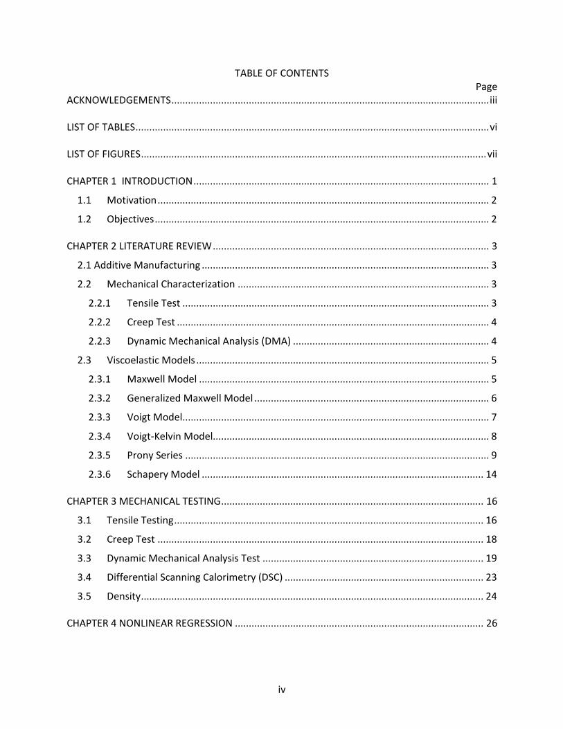
TABLE OF CONTENTS Page

ACKNOWLEDGEMENTS ................................................................................................................... iii

LIST OF TABLES ................................................................................................................................ vi

LIST OF FIGURES ............................................................................................................................. vii

CHAPTER 1 INTRODUCTION ........................................................................................................... 1

1.1 Motivation ........................................................................................................................ 2

1.2 Objectives ......................................................................................................................... 2

CHAPTER 2 LITERATURE REVIEW .................................................................................................... 3

2.1 Additive Manufacturing ........................................................................................................ 3

2.2 Mechanical Characterization ........................................................................................... 3

2.2.1 Tensile Test ............................................................................................................... 3

2.2.2 Creep Test ................................................................................................................. 4

2.2.3 Dynamic Mechanical Analysis (DMA) ....................................................................... 4

2.3 Viscoelastic Models .......................................................................................................... 5

2.3.1 Maxwell Model ......................................................................................................... 5

2.3.2 Generalized Maxwell Model ..................................................................................... 6

2.3.3 Voigt Model ............................................................................................................... 7

2.3.4 Voigt-Kelvin Model.................................................................................................... 8

2.3.5 Prony Series .............................................................................................................. 9

2.3.6 Schapery Model ...................................................................................................... 14

CHAPTER 3 MECHANICAL TESTING ............................................................................................... 16

3.1 Tensile Testing ................................................................................................................ 16

3.2 Creep Test ...................................................................................................................... 18

3.3 Dynamic Mechanical Analysis Test ................................................................................ 19

3.4 Differential Scanning Calorimetry (DSC) ........................................................................ 23

3.5 Density ............................................................................................................................ 24

CHAPTER 4 NONLINEAR REGRESSION .......................................................................................... 26

iv

CHAPTER 5 LINEAR VISCOELASTIC MODELS ................................................................................. 28

5.1 Maxwell Model ................................................................................................................... 28

5.2 Voigt-Kelvin Model ......................................................................................................... 30

5.3 Prony Series .................................................................................................................... 34

CHAPTER 6 NON-LINEAR VISCOELASTIC MODEL .......................................................................... 39

CHAPTER 7 VALIDATION OF MODEL ............................................................................................. 46

CHAPTER 8 CONCLUSIONS AND FUTURE WORK .......................................................................... 55

REFERENCES .................................................................................................................................. 56

v

LIST OF TABLES

Table 1 : Different strain rates and speed of crosshead ............................................................... 17

Table 2 : Young's Modulus and Yield Strength as a function of strain rate .................................. 18

Table 3 : Density of Procast material ............................................................................................ 25

Table 4 : Material Parameters for Maxwell Model ....................................................................... 28

Table 5: Material Parameters for Voigt-Kelvin Model .................................................................. 31

Table 6 : Creep Material Parameters for Prony Series ................................................................ 36

Table 7 : Material Parameters for Schapery Model ..................................................................... 42

Table 8 : Polynomial Constants for Nonlinear Material Paramters ............................................. 44

vi

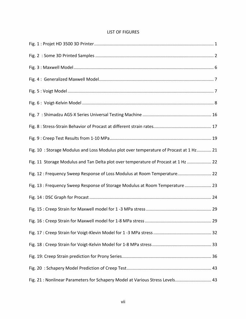
LIST OF FIGURES

Fig. 1 : Projet HD 3500 3D Printer ................................................................................................... 1

Fig. 2 : Some 3D Printed Samples .................................................................................................. 2

Fig. 3 : Maxwell Model .................................................................................................................... 6

Fig. 4 : Generalized Maxwell Model ............................................................................................... 7

Fig. 5 : Voigt Model ......................................................................................................................... 7

Fig. 6 : Voigt-Kelvin Model ............................................................................................................. 8

Fig. 7 : Shimadzu AGS-X Series Universal Testing Machine ......................................................... 16

Fig. 8 : Stress-Strain Behavior of Procast at different strain rates................................................ 17

Fig. 9 : Creep Test Results from 1-10 MPa .................................................................................... 19

Fig. 10 : Storage Modulus and Loss Modulus plot over temperature of Procast at 1 Hz ............ 21

Fig. 11 Storage Modulus and Tan Delta plot over temperature of Procast at 1 Hz .................... 22

Fig. 12 : Frequency Sweep Response of Loss Modulus at Room Temperature ............................ 22

Fig. 13 : Frequency Sweep Response of Storage Modulus at Room Temperature ...................... 23

Fig. 14 : DSC Graph for Procast ..................................................................................................... 24

Fig. 15 : Creep Strain for Maxwell model for 1 -3 MPa stress ...................................................... 29

Fig. 16 : Creep Strain for Maxwell model for 1-8 MPa stress ....................................................... 29

Fig. 17 : Creep Strain for Voigt-Klevin Model for 1 -3 MPa stress ................................................ 32

Fig. 18 : Creep Strain for Voigt-Kelvin Model for 1-8 MPa stress ................................................. 33

Fig. 19: Creep Strain prediction for Prony Series .......................................................................... 36

Fig. 20 : Schapery Model Prediction of Creep Test ...................................................................... 43

Fig. 21 : Nonlinear Parameters for Schapery Model at Various Stress Levels .............................. 43

vii

Fig. 22 : Strain-Rate Dependent Tensile Test Data Including Yielding Region .............................. 46

Fig 23 : Validation for Maxwell Model at Various Strain Rates .................................................... 47

Fig. 24 : Validation for Voigt-Kelvin Model at Various Strain Rates ............................................. 47

Fig. 25 : Validation for Prony Series at Various Strain Rates ........................................................ 48

Fig. 26 : Validation for Schapery Model at Various Strain Rates .................................................. 49

Fig. 27 : Loss Modulus response for Maxwell model ................................................................... 50

Fig. 28 : Loss Modulus response for Voigt-Kelvin model ............................................................. 50

Fig. 29 : Loss Modulus response for Prony model ....................................................................... 51

Fig. 30 : Loss Modulus response for Schapery Model .................................................................. 51

Fig. 31 : Storage Modulus response for Maxwell model .............................................................. 52

Fig. 32 : Storage Modulus response for Voigt-Kelvin model ....................................................... 53

Fig. 33 : Storage Modulus response for Prony Series ................................................................... 53

Fig. 34 : Storage Modulus response for Schapery model ............................................................. 54

viii

CHAPTER 1

INTRODUCTION

Recent development of additive manufacturing technologies has led to a lack of

information on the base materials being used. A need arises to know the mechanical behaviors

of these base materials so that it can be linked with macroscopic mechanical behaviors of 3D

network structures manufactured from the 3D printer. The base material used by our 3D

printer is Procast. The objective of my research is to investigate non-linear stress-strain

behaviors of the Procast obtained from the 3D printer.

Fig. 1 : Projet HD 3500 3D Printer

For this purpose, different mechanical tests are conducted on Procast such as tensile

test, and creep test. Some dynamic mechanical analysis is also being carried out. For this

purpose, a 3D CAD model is made using ProE and 3D printed using Projet HD3500 plus Fig. 1.

For post-processing, a Projet finisher oven is used to melt the support material, and digital

ultrasonic cleaner is used for cleaning the remaining support material. Tensile and creep tests

1

are performed using Shimadzu AGS-X series Universal Testing Machine following ASTM

standards [1]-[5][8][9]. Rheometric Scientific equipment is used to carry out dynamic

mechanical analysis. Experimental data is fitted using different viscoelastic models both in time

domain and frequency domain. Validation of the data is carried out using experimental test

data and viscoelastic model data.

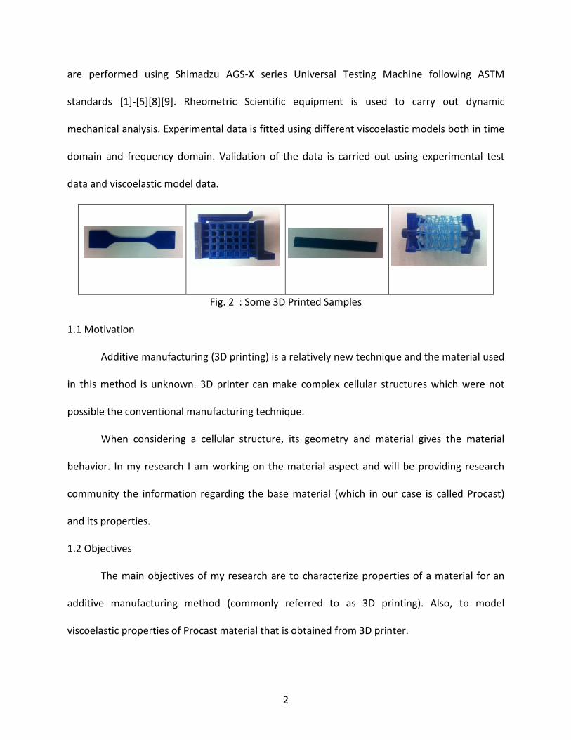
Fig. 2 : Some 3D Printed Samples

1.1 Motivation

Additive manufacturing (3D printing) is a relatively new technique and the material used

in this method is unknown. 3D printer can make complex cellular structures which were not

possible the conventional manufacturing technique.

When considering a cellular structure, its geometry and material gives the material

behavior. In my research I am working on the material aspect and will be providing research

community the information regarding the base material (which in our case is called Procast)

and its properties.

1.2 Objectives

The main objectives of my research are to characterize properties of a material for an

additive manufacturing method (commonly referred to as 3D printing). Also, to model

viscoelastic properties of Procast material that is obtained from 3D printer.

2

CHAPTER 2

LITERATURE REVIEW

2.1 Additive Manufacturing

Additive manufacturing is a method in which 3D solid objects are printed using a 3D

printer. In common terminology, additive manufacturing is also termed as 3D printing. The

general principle of additive manufacturing is layer by layer deposition of base material to make

3D parts. Additive manufacturing uses a 3D CAD model as a soft copy for 3D part. The

corresponding CAD file is converted into STL format which is the required format for the 3D

printer [1]. Upon receiving the STL file, the 3D printer starts printing the 3D part layer by layer.

There are differing types of printing process available [2]; the following two processes

are used by our Projet HD 3500 plus, 3D Systems printer.

a) Fused deposition modeling (FDM): In this method, layer by layer deposition of base

material is made by the 3D printer.

b) Stereolithography (SLA): This process uses a laser to solidify the base material as it is

being printed by FDM method.

2.2 Mechanical Characterization

Since 3D printing is a new technique, and base materials being used for it are relatively

new as well, a need arises to conduct different mechanical tests in order to find their

mechanical properties.

2.2.1 Tensile Test

Tensile tests were carried out using ASTM Standards D412 [1] and D638 [5]. For our

Procast material, dumbbell shaped specimen Fig. 2 was printed using Projet HD3500 Fig. 1. The

3

same dimensions were considered for Procast as Die C in ASTM standard D412 [1]. Once the

sample is printed, it is placed in the Projet finisher oven to melt the support material; in our

case it is wax. The Procast sample is further cleaned using Digital Ultrasonic Cleaner, and the

material obtained is dried by placing it in a desiccator.

For the tensile test, Shimadzu AGS-X series Universal Testing Machine Fig. 7 is used with

a load cell of 5kN. The test is conducted at room temperature 23 ± 2°C as per ASTM standards.

For different strain rates, the cross-head speed of the machine is adjusted to obtain the desired

strain rate.

2.2.2 Creep Test

Creep tests were carried out using Shimadzu AGS-X series Universal Testing Machine. In

a creep test, stress is held constant for some time duration at a specified temperature. We

conducted the test using different stress levels at room temperature 23 ± 2°C for 1800 seconds.

ASTM Standard D2990 [3] was followed in preparing the sample. The sample dimension was in

standing with Type 1 in ASTM Standard D638 [5].

2.2.3 Dynamic Mechanical Analysis (DMA)

Dynamic mechanical properties refer to the response of the material when it is

subjected to dynamic loading. These properties may be expressed in terms of a storage

modulus, loss modulus and a damping term.

Temperature sweep test is conducted where we study the response of the material at

fixed frequency over a wide range of temperature. This temperature sweep allows in studying

the transitions in the material including the glass transition temperature (𝑇𝑇𝑔𝑔).

4

A Frequency sweep test is conducted where we study the response of the material at

fixed temperature but over a wide range of frequencies, we use this data for time temperature

superposition. We find the material properties by the following equations

𝑆𝑡𝑜𝑟𝑎𝑔𝑒 𝑀𝑜𝑑𝑢𝑙𝑢𝑠 (E’) = 𝜎𝑜Є𝑜𝑐𝑜𝑠𝛿 (2. 1)

𝐿𝑜𝑠𝑠 𝑀𝑜𝑑𝑢𝑙𝑢𝑠 (E’’) = 𝜎𝑜Є𝑜𝑠𝑖𝑛𝛿 (2. 2)

𝑃ℎ𝑎𝑠𝑒 𝑎𝑛𝑔𝑙𝑒 ∶ 𝑇𝑇𝑎𝑛(𝑑𝑒𝑙𝑡𝑎) = E’’E’

(2. 3)

2.3 Viscoelastic Models

Viscoelasticity is made up of two words: viscous and elastic. If a material exhibits both

elastic and viscous nature, then it is termed as viscoelasticity, and such material exhibits a time-

dependent strain. A viscoelastic material has an elastic component and a viscous component.

This viscous component gives a time-dependent strain. The elastic component is modeled as

spring (𝜎 = 𝐸𝜀), while the viscous component is modeled as dashpot (𝜎 = 𝜂 𝑑𝜀𝑑𝑡

)

There are various viscoelastic material models that give a good time dependent

response of the material. Few viscoelastic material models are studied here.

2.3.1 Maxwell Model

Maxwell model is the simplest model that gives linear viscoelastic material response

[11] [13]. In this model, spring is connected in a series with a dashpot. Here, strain in both the

elements is different while stress remains same 𝜎𝑇𝑂𝑇𝐴𝐿 = 𝜎𝐷 = 𝜎𝑆

Total strain is the sum of strains in spring and dashpot 𝜀𝑇𝑂𝑇𝐴𝐿 = 𝜀𝐷 + 𝜀𝑆

5

Fig. 3 : Maxwell Model

To obtain strain rate,

𝑑𝜀𝑇𝑂𝑇𝐴𝐿𝑑𝑡

=𝑑𝜀𝐷𝑑𝑡

+𝑑𝜀𝑆𝑑𝑡

=𝜎𝜂

+1𝐸𝑑𝜎𝑑𝑡

(2. 4)

𝜀̇ =𝜎𝜂

+�̇�𝐸

(2. 5)

For Stress Relaxation test, the above equations becomes

0 =𝜎𝜂

+�̇�𝐸

(2. 6)

�̇�𝐸

= −𝜎𝜂

(2. 7)

𝑑𝜎𝜎

= −𝐸𝜂𝑑𝑡 (2. 8)

𝜎 = 𝜎𝑜𝑒−𝑡 𝜏� (2. 9)

Here, τ is the relaxation time given by 𝜏 = 𝜂𝐸�

And Relaxation Modulus 𝐸(𝑡) is given by

𝐸(𝑡) = 𝐸𝑒−𝑡 𝜏� (2. 10)

And for Creep Compliance,

𝐷(𝑡) = 𝐷(1 + 𝑡 𝜏� ) (2. 11)

2.3.2 Generalized Maxwell Model

Generalized Maxwell model is obtained by adding parallel combinations of n Maxwell

units. This model is used to model relaxation behavior [12]-[13].

𝐸

𝜂

6

Fig. 4 : Generalized Maxwell Model

The relation for stress relaxation for the generalized Maxwell model is given by

𝐸(𝑡) = �𝐸𝑖𝑒−𝑡 𝜏𝑖�

𝑛

𝑖=1

(2. 12)

The equation for Generalized Maxwell model in frequency domain is given by

(𝑆𝑡𝑜𝑟𝑎𝑔𝑒 𝑀𝑜𝑑𝑢𝑙𝑢𝑠)𝐸′(𝜔) = ��𝐸𝑖𝜏𝑖2𝜔2

1 + 𝜏𝑖2𝜔2�𝑛

𝑖=1

(2. 13)

(𝐿𝑜𝑠𝑠 𝑀𝑜𝑑𝑢𝑙𝑢𝑠)𝐸′′(𝜔) = ��𝐸𝑖𝜏𝑖𝜔

1 + 𝜏𝑖2𝜔2�𝑛

𝑖=1

(2. 14)

2.3.3 Voigt Model

Voigt model is another type of linear viscoelastic material model in which spring and

dashpot are connected in parallel.

Fig. 5 : Voigt Model

Here, stress is different in both the elements while strain remains same: 𝜀𝑇𝑂𝑇𝐴𝐿 = 𝜀𝐷 = 𝜀𝑆

𝐸 𝜂

7

Total stress is sum of stresses in spring and dashpot: 𝜎𝑇𝑂𝑇𝐴𝐿 = 𝜎𝐷 + 𝜎𝑆

𝜎(𝑡) = 𝐸 𝜀(𝑡) + 𝜂𝑑𝜀(𝑡)𝑑𝑡

(2. 15)

For creep test,

𝜎𝑜 = 𝐸 𝜀(𝑡) + 𝜂𝑑𝜀(𝑡)𝑑𝑡

(2. 16)

𝜀(𝑡) =𝜎𝑜𝐸�1 − 𝑒−𝑡 𝜏� � (2. 17)

Here, τ is the relaxation time given by 𝜏 = 𝜂𝐸�

Thus, creep compliance is given by

𝐷(𝑡) = 𝐷 �1 − 𝑒−𝑡 𝜏� � (2. 18)

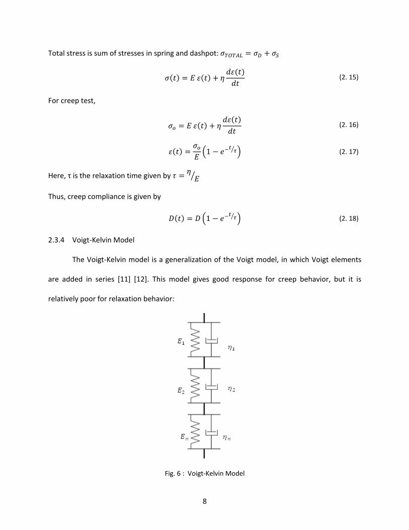
2.3.4 Voigt-Kelvin Model

The Voigt-Kelvin model is a generalization of the Voigt model, in which Voigt elements

are added in series [11] [12]. This model gives good response for creep behavior, but it is

relatively poor for relaxation behavior:

Fig. 6 : Voigt-Kelvin Model

8

So, for n number of Voigt elements, the creep compliance is given by

𝐷(𝑡) = �𝐷𝑖 �1 − 𝑒−𝑡 𝜏𝑖� �

𝑛

𝑖=1

(2. 19)

Applying Fourier Transformation,

(𝑆𝑡𝑜𝑟𝑎𝑔𝑒 𝑀𝑜𝑑𝑢𝑙𝑢𝑠) 𝐷′(𝜔) = ��𝐷𝑖

1 + 𝜏𝑖2𝜔2�𝑛

𝑖=1

(2. 20)

(𝐿𝑜𝑠𝑠 𝑀𝑜𝑑𝑢𝑙𝑢𝑠) 𝐷′′(𝜔) = �𝐷𝑖 �𝜏𝑖𝜔

1 + 𝜏𝑖2𝜔2�𝑛

𝑖=1

(2. 21)

2.3.5 Prony Series

A common form for the linear viscoelastic response is given by Prony Series by the

following equation [10]:

�𝛼𝑖𝑒−𝑡 𝜏𝑖�

𝑁

𝑖=1

(2. 22)

Here, 𝜏𝑖 are the time constants and 𝛼𝑖 are the exponential coefficients.

In order to determine material parameters, creep and relaxation tests are used mostly.

There are various approaches to determine Prony coefficients; we have used a nonlinear

regression approach to determine the coefficients.

We know that for a relaxation test, its constitutive equation is given by the following equation:

𝜎(𝑡) = 𝑌(𝑡)Є0 (2. 23)

Here, 𝑌(𝑡) is the relaxation function, and its response under Prony Series is given by

𝑌(𝑡) = 𝐸0.�1 −�𝑝𝑖(1 − 𝑒−𝑡 𝜏𝑖�

𝑛

𝑖=1

� (2. 24)

Here,

9

𝑝𝑖 is the ith Prony constant 𝑖 = (1,2,3, … )

𝜏𝑖 is the ith Prony Retardation time constant 𝑖 = (1,2,3, … )

𝐸0 is the instantaneous modulus

When time 𝑡 = 0, 𝑌(0) = 𝐸0

And when time 𝑡 = ∞, 𝑌(∞) = 𝐸∞(1 − ∑𝑝𝑖)

To determine the stress state at a particular time, the deformation history must be

taken into account. For linear viscoelastic materials, a superposition of hereditary integrals

gives a time dependent response. In the case for stress relaxation, the specimen is under no

strain level prior to time 𝑡 = 0, at which a strain is applied and its corresponding stress

response for time 𝑡 > 0 is given by

𝜎(𝑡) = Є0𝑌(𝑡) + � 𝑌(𝑡 − 𝜉)𝑑Є(𝜉)𝑑𝜉

𝑑𝜉𝑡

0 (2. 25)

Here, 𝑌(𝑡) is the relaxation function and 𝑑Є(𝜉)𝑑𝜉

is the strain rate.

The process in general relaxation test is divided into 2 segments [10]: loading response

(increasing strain rate) and constant strain response (zero strain rate). Their functions are given

below:

Є(𝑡) = �Є1𝑡

(𝑡1 − 𝑡0)� ; 𝑡0 < 𝑡 < 𝑡1

Є1 ; 𝑡1 < 𝑡 < 𝑡2�

𝑑Є𝑑𝑡

= �Є1

(𝑡1 − 𝑡0)� ; 𝑡0 < 𝑡 < 𝑡1

0 ; 𝑡1 < 𝑡 < 𝑡2�

Here, Є0 = 0, Є1 is the strain level at which the strain is kept constant, and 𝑡0 = 0

10

Using the above strain response, the stress function for the loading response can be given as

[10]

Step 1(𝒕𝟎 < 𝑡 ≤ 𝒕𝟏)

𝜎1(𝑡) = Є0𝑌(𝑡) + � 𝑌(𝑡 − 𝜉)𝑑Є(𝜉)𝑑𝜉

𝑑𝜉𝑡

0 (2. 26)

𝜎1(𝑡) = 0 + � 𝐸0. �1 −�𝑝𝑖(1 − 𝑒−(𝑡−𝜉)

𝜏𝑖�𝑛

𝑖=1

�Є1𝑡1

𝑑𝜉𝑡

0 (2. 27)

𝜎1(𝑡) = 𝐸0Є1𝑡1

� �1 −�𝑝𝑖(1 − 𝑒−(𝑡−𝜉)

𝜏𝑖�𝑛

𝑖=1

� 𝑑𝜉𝑡

0 (2. 28)

𝜎1(𝑡) = 𝐸0Є1𝑡1

� �1 −�𝑝𝑖

𝑛

𝑖=1

+ �𝑝𝑖𝑒−(𝑡−𝜉)

𝜏𝑖�𝑛

𝑖=1

� 𝑑𝜉𝑡

0 (2. 29)

𝜎1(𝑡) = 𝐸0Є1𝑡1

�𝜉 −�𝑝𝑖𝜉𝑛

𝑖=1

+ �𝜏𝑖𝑝𝑖𝑒−(𝑡−𝜉)

𝜏𝑖�𝑛

𝑖=1

�0

𝑡

(2. 30)

𝜎1(𝑡) = 𝐸0Є1𝑡1

�𝑡 −�𝑝𝑖𝑡 +�𝑝𝑖𝜏𝑖 −�𝑝𝑖𝜏𝑖𝑒−𝑡 𝜏𝑖� � (2. 31)

Here, n is the number of terms in the Prony Series.

Step 2(𝒕𝟏 < 𝑡 ≤ 𝒕𝟐)

In this step, the strain is kept constant.

𝜎2(𝑡) = Є0𝑌(𝑡) + � 𝑌(𝑡 − 𝜉)𝑑Є(𝜉)𝑑𝜉

𝑑𝜉𝑡1−

0+ � 𝑌(𝑡 − 𝜉)

𝑑Є(𝜉)𝑑𝜉

𝑑𝜉𝑡

𝑡1+ (2. 32)

𝜎2(𝑡) = 0 +𝐸0Є1𝑡1

�𝜉 −�𝑝𝑖𝜉𝑛

𝑖=1

+ �𝜏𝑖𝑝𝑖𝑒−(𝑡−𝜉)

𝜏𝑖�𝑛

𝑖=1

�0

𝑡1

+ 0 (2. 33)

𝜎2(𝑡) = 𝐸0Є1𝑡1

�𝑡1 −�𝑝𝑖𝑡1 +�𝑝𝑖𝜏𝑖𝑒−(𝑡−𝑡1)

𝜏𝑖� −�𝑝𝑖𝜏𝑖𝑒−𝑡 𝜏𝑖� � (2. 34)

11

Using a non-linear regression technique [10], the above stress function can be determined by a

stress relaxation test.

To get material response in frequency domain for Prony Series, we apply Fourier

transformation. Prony Series is represented in terms of shear relaxation modulus by the

following expression [20]:

𝑔𝑅(𝑡) = 1 −�𝑔𝑖 �1 − 𝑒−𝑡 𝜏𝑖� �

𝑁

𝑖=1

(2. 35)

Here, 𝑔𝑖 and 𝜏𝑖 are material parameters and 𝑔𝑅(𝑡) is the dimensionless relaxation modulus

given by

𝑔𝑅(𝑡) =𝐺𝑅(𝑡)𝐺0

(2. 36)

Apply Fourier Transformation:

(𝑆𝑡𝑜𝑟𝑎𝑔𝑒 𝑀𝑜𝑑𝑢𝑙𝑢𝑠) 𝐺′(𝜔) = 𝐺0 �1 −�𝑔𝑖

𝑁

𝑖=1

� + 𝐺0�𝑔𝑖

𝑁

𝑖=1

�𝜏𝑖2𝜔2

1 + 𝜏𝑖2𝜔2� (2. 37)

(𝐿𝑜𝑠𝑠 𝑀𝑜𝑑𝑢𝑙𝑢𝑠) 𝐺′′(𝜔) = 𝐺0�𝑔𝑖

𝑁

𝑖=1

�𝜏𝑖𝜔

1 + 𝜏𝑖2𝜔2� (2. 38)

We know that for creep compliance [10],

Є(𝑡) = 𝐽(𝑡)𝜎0 (2. 39)

Here, 𝐽(𝑡) is the creep compliance function and its response under Prony Series is given by

𝐽(𝑡) = 𝐽0.�1 −�𝑝𝑖𝑒−𝑡 𝜏𝑖�

𝑛

𝑖=1

� (2. 40)

Є(𝑡) = 𝜎0𝐽(𝑡) + � 𝐽(𝑡 − 𝜉)𝑑𝜎(𝜉)𝑑𝜉

𝑑𝜉𝑡

0 (2. 41)

12

𝜎(𝑡) = �𝜎1𝑡

(𝑡1 − 𝑡0)� ; 𝑡0 < 𝑡 < 𝑡1

𝜎1 ; 𝑡1 < 𝑡 < 𝑡2�

𝑑𝜎𝑑𝑡

= �𝜎1

(𝑡1 − 𝑡0)� ; 𝑡0 < 𝑡 < 𝑡1 0 ; 𝑡1 < 𝑡 < 𝑡2

�

Here, 𝜎0 = 0, 𝜎1 is the stress level at which the stress is kept constant, and 𝑡0 = 0

Step 1(𝒕𝟎 < 𝒕 ≤ 𝒕𝟏)

Є1(𝑡) = 𝜎0𝐽(𝑡) + � 𝐽(𝑡 − 𝜉)𝑑𝜎(𝜉)𝑑𝜉

𝑑𝜉𝑡

0 (2. 42)

Є1(𝑡) = 0 + � 𝐽0.�1 −�𝑝𝑖𝑒−(𝑡−𝜉)

𝜏𝑖�𝑛

𝑖=1

�𝜎1𝑡1

𝑑𝜉𝑡

0 (2. 43)

Є1(𝑡) = 0 + � 𝐽0.�1 −�𝑝𝑖𝑒−(𝑡−𝜉)

𝜏𝑖�𝑛

𝑖=1

�𝜎1𝑡1

𝑑𝜉𝑡

0 (2. 44)

Є1(𝑡) = 𝐽0𝜎1𝑡1

�𝜉 −�𝜏𝑖𝑝𝑖𝑒−(𝑡−𝜉)

𝜏𝑖�𝑛

𝑖=1

�0

𝑡

(2. 45)

Є1(𝑡) = 𝐽0𝜎1𝑡1

�𝑡 −�𝑝𝑖𝜏𝑖 +�𝑝𝑖𝜏𝑖𝑒−𝑡 𝜏𝑖� � (2. 46)

Step 2(𝒕𝟏 < 𝒕 ≤ 𝒕𝟐)

In this step, the stress is kept constant.

Є2(𝑡) = 𝜎0𝐽(𝑡) + � 𝐽(𝑡 − 𝜉)𝑑𝜎(𝜉)𝑑𝜉

𝑑𝜉𝑡1−

0+ � 𝐽(𝑡 − 𝜉)

𝑑𝜎(𝜉)𝑑𝜉

𝑑𝜉𝑡

𝑡1+ (2. 47)

Є2(𝑡) = 0 +𝐽0𝜎1𝑡1

�𝜉 −�𝜏𝑖𝑝𝑖𝑒−(𝑡−𝜉)

𝜏𝑖�𝑛

𝑖=1

�0

𝑡1

+ 0 (2. 48)

Є2(𝑡) = 𝐽0𝜎1𝑡1

�𝑡1 −�𝑝𝑖𝜏𝑖𝑒−(𝑡−𝑡1)

𝜏𝑖� + �𝑝𝑖𝜏𝑖𝑒−𝑡 𝜏𝑖� � (2. 49)

13

2.3.6 Schapery Model

Schapery model is used to model the behavior of non-linear viscoelastic materials. We

know that for creep test,

Є𝜎

= 𝐷(𝑡) (2. 50)

Here, 𝐷(𝑡) is the creep compliance. For this creep test, the stress-strain equation is given by

[18]- [19]:

Є = 𝐷0𝜎 + 𝛥𝐷(𝑡)𝜎 (2. 51)

Here, 𝐷0 is the initial value of compliance and

𝛥𝐷(𝑡) = 𝐷(𝑡) − 𝐷0 (2. 52)

Similar response can be obtained for stress relaxation test.

When we have creep test data, i.e. 𝐷(𝑡) is known, we can calculate strain by using Boltzmann

superposition principal which is given by,

Є = 𝐷0𝜎 + � 𝛥𝐷(𝑡 − 𝜏)𝑡

0

𝑑𝜎𝑑𝜏

𝑑𝜏 (1) (2. 53)

This was the linear response of the material [14]-[19], slight changes are to made in the above

equation to obtain nonlinear constitutive equation, which is given below

Є(𝑡) = 𝑔0𝐷0𝜎 + 𝑔1 � 𝛥𝐷[𝜓(𝑡) − 𝜓′(𝜏)]𝑡

0

𝑑𝑔2𝜎𝑑𝜏

𝑑𝜏 (2) (2. 54)

The above equation gives 1-D representation for Schapery model. Here, 𝐷0 and 𝛥𝐷(𝜓) are the

instantaneous and transient linear viscoelastic creep compliance components which have been

defined previously, and 𝜓 is reduced-time given by

14

𝜓 = �𝑑𝑡′

𝑎𝜎[𝜎(𝑡′)]

𝑡

0

(2. 55)

And

𝜓′ = 𝜓(𝜏) = �𝑑𝑡′

𝑎𝜎[𝜎(𝑡′)]

𝜏

0

(2. 56)

By comparing equations (2. 53 and (2. 54 and 1 we see that 𝑔0,𝑔1,𝑔2,𝑎𝜎 = 1 when the stress is

sufficiently small. For case of creep test, constant stress 𝜎 is used and the strain rate 𝑑𝑔𝑔2𝜎𝑑𝜏

𝑑𝜏

goes to zero. So the equation modifies to [14]-[19]

𝐷𝑛 =Є𝜎

= 𝑔0𝐷0 + 𝑔1𝑔2𝛥𝐷 �𝑡𝑎𝜎� (2. 57)

If we have 𝑔0,𝑔1,𝑔2,𝑎𝜎 = 1 then above equation becomes

𝐷𝑛 =Є𝜎

= 𝐷0 + 𝛥𝐷(𝑡) (2. 58)

This is the response for linear Schapery model. The transient tensile component 𝛥𝐷(𝜓) is

expressed in terms of Prony series [17]

𝛥𝐷(𝜓) = �𝐷𝑛[1 − exp (−𝜆𝑛𝜓)]𝑁

1

(2. 59)

Here, 𝐷𝑛 and 𝜆𝑛 are Prony constants which can be determined by tensile creep compliance

data and non-linear material parameter 𝑔0,𝑔1,𝑔2,𝑎𝜎 can be determined by creep-recovery

tests.

15

CHAPTER 3

MECHANICAL TESTING

In this chapter we found mechanical properties of 3D printed material Procast obtained

from a 3D printer. Procast is a new 3D material, and its properties are unknown. Tensile tests

are conducted at 4 different strain rates to study the effect of elastic modulus. Stress relaxation

and creep test are also conducted to study the viscoelastic response of the material.

3.1 Tensile Testing

For Uniaxial Testing Shimadzu AGS-X Series universal Testing Machine Fig. 7 is used with

a load cell of 5kN. The maximum speed to elongate with the current universal testing machine

was 1000 mm/sec.

Fig. 7 : Shimadzu AGS-X Series Universal Testing Machine

A uniaxial tension test was performed with sample dimensions as per ASTM D412

standards [1]. Testing speed was taken from 1.5 mm/sec to 75 mm/sec, which corresponds to a

strain rate of 0.001 sec−1 to 0.05 sec−1.

16

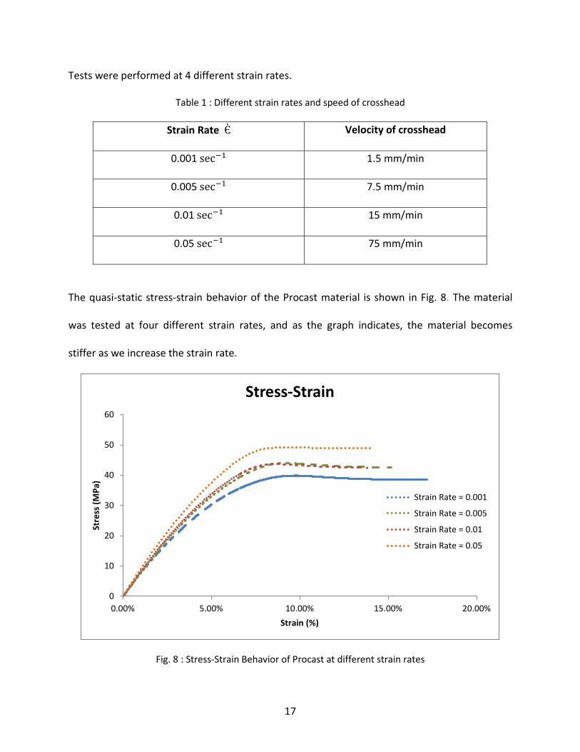
Tests were performed at 4 different strain rates.

Table 1 : Different strain rates and speed of crosshead

Strain Rate Є̇ Velocity of crosshead

0.001 sec−1 1.5 mm/min

0.005 sec−1 7.5 mm/min

0.01 sec−1 15 mm/min

0.05 sec−1 75 mm/min

The quasi-static stress-strain behavior of the Procast material is shown in Fig. 8. The material

was tested at four different strain rates, and as the graph indicates, the material becomes

stiffer as we increase the strain rate.

Fig. 8 : Stress-Strain Behavior of Procast at different strain rates

0

10

20

30

40

50

60

0.00% 5.00% 10.00% 15.00% 20.00%

Stre

ss (M

Pa)

Strain (%)

Stress-Strain

Strain Rate = 0.001

Strain Rate = 0.005

Strain Rate = 0.01

Strain Rate = 0.05

17

The material response can also be studied from Table 2, where Young’s modulus and yield

strength are listed at various strain rates.

Table 2 : Young's Modulus and Yield Strength as a function of strain rate

Strain Rate

(𝒔𝒆𝒄−𝟏)

Young’s Modulus

(𝑮𝐏𝐚)

Yield Strength

(𝐌𝐏𝐚)

Yield Force

(𝐍)

0.001 0.727±0.051 16.33±3 184.66±34.7

0.005 0.77±0.05 16.66±2.62 188.66±29.17

0.01 0.788±0.056 18±2.9 203.33±33.29

0.05 0.831±0.059 19±1.63 222±17.57

From Fig. 8, we can see that initially the material experiences a linear response. After some

time, it undergoes non-linear deformation and fails around 10-12% strain. As we increase the

strain rate the material becomes more stiff and its Young’s modulus increases which is given in

Table 2.

3.2 Creep Test

Creep tests were carried out Shimadzu AGS-X Series Universal Testing Machine Fig. 7.

Procast sample was hold at different stress levels (1-10 MPa) for 1800 seconds.

Their responses are given below:

18

Fig. 9 : Creep Test Results from 1-10 MPa

Fig. 9 shows strain versus time response for creep test. It can be seen from these figures that as

the stress values are held constant, strain increases exponentially for that period.

3.3 Dynamic Mechanical Analysis Test

The DMA test was conducted using a Rheometric Scientific Equipment in bending mode.

The sample was placed on a clamping fixture and the strain amplitude was applied with by a

movable clamp at the center of the sample. Distance between clamps was 25 mm. The

response from the sample was measured as stress. The dynamic modulus (E’), dynamic loss

modulus (E”) was determined by phase angle, the strain applied and the measured stress and

their formula is given below [7]-[8].

0.00%

0.50%

1.00%

1.50%

2.00%

2.50%

0 500 1000 1500 2000

Stra

in

Time (sec)

Strain at 1-10 MPa

1 MPa2 MPa3 MPa4 MPa5 MPa6 MPa7 MPa8 MPa9 MPa10 MPa

19

𝑆𝑡𝑜𝑟𝑎𝑔𝑒 𝑀𝑜𝑑𝑢𝑙𝑢𝑠 (E’) = 𝜎𝑜Є𝑜𝑐𝑜𝑠𝛿 (3. 1)

𝐿𝑜𝑠𝑠 𝑀𝑜𝑑𝑢𝑙𝑢𝑠 (E’’) = 𝜎𝑜Є𝑜𝑠𝑖𝑛𝛿 (3. 2)

𝑃ℎ𝑎𝑠𝑒 𝑎𝑛𝑔𝑙𝑒 ∶ 𝑇𝑇𝑎𝑛(𝑑𝑒𝑙𝑡𝑎) = E’’E’

(3. 3)

Initially a strain sweep test was conducted in order to find the strain amplitude that can

be used for the material to follow Hook’s Law. Strain amplitude used for this polyurethane was

0.005%. Once strain amplitude was found a dynamic temperature sweep test was conducted at

a frequency of 1 Hz over a temperature range of -100 °C to 150 °C with a scanning rate of

3°C 𝑚𝑖𝑛−1. A sinusoidal strain was applied and material response was measured as stress. By

approximating the applied sinusoidal strain wave with a triangular strain wave, the average

strain was calculated as ∈̇=2 ∈ 𝜔.

Fig. 10 gives temperature sweep response for Procast at 1 Hz. Maximum value of E’ is

observed in the region of -65°C till -35°C which is in the order of 13 GPa. The values of E’ is 9.4

GPa at around 25°C. It can be clearly seen that E’ decreases around 25°C and this steep

decrease is observed till 100°C. From 100°C till 150°C material maintains almost a constant

value E’ of 0.1-0.2 GPa so this can be taken In account where material application comes in.

20

Fig. 10 : Storage Modulus and Loss Modulus plot over temperature of Procast at 1 Hz

Fig. 11 gives response for Tan Delta curve response for Procast at 1 Hz. Since, there is an

inverse relation between Storage Modulus (E’) and Tan δ given by Tan δ = Eʹ𝐸ʹʹ

, so Tan δ peak is

observed corresponding to decrease in E’ in similar temperature range Fig. 11. So, peak in Tan

delta region gives material glass transition 𝑇𝑇𝑔𝑔 value, which in for Procast is around 81°C.

0

0.1

0.2

0.3

0.4

0.5

0.6

0.7

0.8

0.9

1

0.1

1

10

100

-150 -100 -50 0 50 100 150 200

E" (G

Pa)

E' (G

Pa)

Temp (C)

Temperature Sweep @ 1 Hz

E'(Storage Modulus)

E''(Loss Modulus)

21

Fig. 11 Storage Modulus and Tan Delta plot over temperature of Procast at 1 Hz

A frequency sweep test 0.01 Hz to 80 Hz on Procast material was also conducted at

room temperature (25°C) using same material dimension as stated in ASTM Standard.

Fig. 12 : Frequency Sweep Response of Loss Modulus at Room Temperature

0.01

0.1

1

0.1

1

10

100

-150 -100 -50 0 50 100 150 200

Tan_

Delta

E' (G

Pa)

Temp (C)

Temperature Sweep @ 1 Hz E'(Storage Modulus)Tan_Delta

0

0.02

0.04

0.06

0.08

0.1

0.12

0.14

0.16

0.00E+00

1.00E+08

2.00E+08

3.00E+08

4.00E+08

5.00E+08

6.00E+08

7.00E+08

8.00E+08

0 20 40 60 80 100

Tan_

Delta

E'' (

Pa)

Freq (Hz)

Loss Modulus

Tan_Delta

22

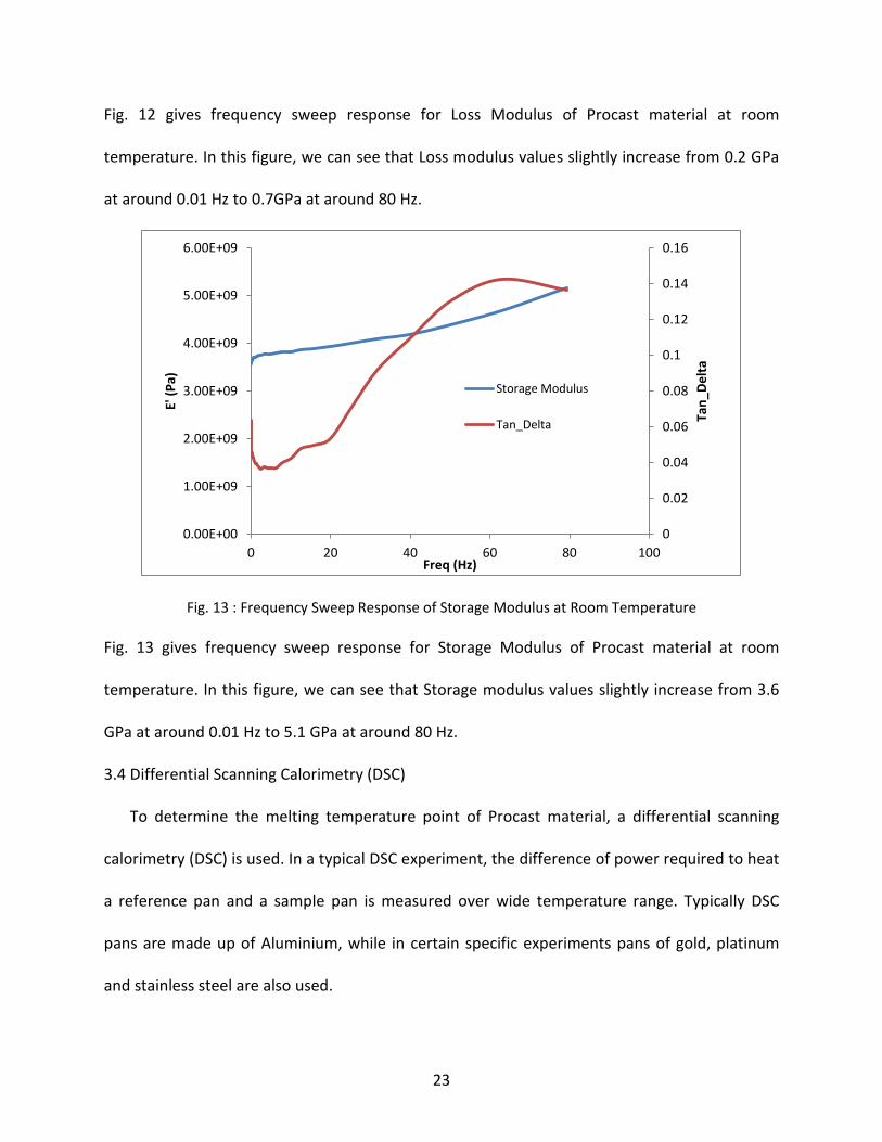
Fig. 12 gives frequency sweep response for Loss Modulus of Procast material at room

temperature. In this figure, we can see that Loss modulus values slightly increase from 0.2 GPa

at around 0.01 Hz to 0.7GPa at around 80 Hz.

Fig. 13 : Frequency Sweep Response of Storage Modulus at Room Temperature

Fig. 13 gives frequency sweep response for Storage Modulus of Procast material at room

temperature. In this figure, we can see that Storage modulus values slightly increase from 3.6

GPa at around 0.01 Hz to 5.1 GPa at around 80 Hz.

3.4 Differential Scanning Calorimetry (DSC)

To determine the melting temperature point of Procast material, a differential scanning

calorimetry (DSC) is used. In a typical DSC experiment, the difference of power required to heat

a reference pan and a sample pan is measured over wide temperature range. Typically DSC

pans are made up of Aluminium, while in certain specific experiments pans of gold, platinum

and stainless steel are also used.

0

0.02

0.04

0.06

0.08

0.1

0.12

0.14

0.16

0.00E+00

1.00E+09

2.00E+09

3.00E+09

4.00E+09

5.00E+09

6.00E+09

0 20 40 60 80 100

Tan_

Delta

E' (P

a)

Freq (Hz)

Storage Modulus

Tan_Delta

23

In our experiment we have used a DSC 6 Perkin Elmer machine. Procast sample was

prepared in Aluminium pans (30µL), weighed and crimped. For reference a black Aluminium

pan was used. Peak observed in the following graph indicated Procast melting temperature

which is 337.5 °C.

Fig. 14 : DSC Graph for Procast

3.5 Density

We also measured density of Procast sample. For this purpose we printed out 5 by 5 by 5

rectangular samples from 3D printer at high definition, ultra high definition and extreme

ultra high definition. Three samples for each resolution level were measured to obtain the

density whose result is given in Table 3. The densities of the three samples are

1125.797±1.356 kg/m3, 1155.503±0.984 kg/m3, and 1162.283±0.835 kg/m3 for High

Definition, Ultra High-Definition, and Extreme Ultra High-Definition resolution respectively.

0

5

10

15

20

25

30

0 50 100 150 200 250 300 350 400 450

Heat

Flo

w (m

W)

Temperature (oC)

DSC Graph for Procast

𝑇𝑇𝑔𝑔 = 97.591 oC

𝑇𝑇𝑚𝑚 = 337.105 oC

24

Table 3 : Density of Procast material

High Definition Ultra High-Definition Extreme Ulta High-Definition

Sample

1

Sample

2

Sample

3

Sample

1

Sample

2

Sample

3

Sample

1

Sample

2

Sample

3

Volume

mm3 124.99 124.248 125.482 124.744 124.744 124.744 124.998 124.747 124.998

Mass

mg 140.67 139.71 141.5 144.15 143.99 144.29 145.17 145.13 145.26

Density

kg/m3 1125.3 1124.44 1127.65 1155.56 1154.27 1156.68 1161.37 1163.39 1162.09

25

CHAPTER 4

NONLINEAR REGRESSION

Nonlinear regression analysis is a technique in which experimental data is modeled by

function which is a combination of material/model parameters. The experimental data is fitted

by using an algorithm or a fitting approach to best predict the behavior. Curve fitting technique

is used to describe experimental data with mathematical equations.

Suppose there is a function y=f(x). Where x is the independent variable and y is dependent

variable, which is measured; and f is the function which uses one or more model parameters to

describe y. Better prediction of these material parameters by any algorithm, the more accurate

the function describes the data. There are many approaches and software available to find out

the best model parameters that gives a good fit. I have used Excel, to obtain my material

parameters. Excel contains the SOLVER function, which comes with every MS office package. It

uses an iterative approach to fit the data with non-linear functions [22][25].

The method used for this approach is called iterative non-linear least square fitting. In a

linear regression (least square approach), we try to minimize the value of squared sum of the

difference between experimental value and predicted/fitted value.

𝑆𝑆 = ��𝑦 − 𝑦𝑓𝑖𝑡�2

𝑛

𝑖=1

(4. 1)

Here, y is the experimental value, 𝑦𝑓𝑖𝑡 is the predicted/fitted value, and SS is the sum of the

squares. The difference between linear regression and non-linear regression is that, in the later

we use iterations to get this SS value to minimum.

26

Starting point for this method is to assume or predict good initial parameters for the

function. This good starting value provides less iteration to compute the function and obtain

best result.

In the first iteration, once we have given some initial starting value, the algorithm runs

the function and obtains some SS value. In second iteration, SOLVER makes small changes in the

initial parameters values and recalculates value of SS.

This method is repeated many times to ensure we have the smallest possible value of

SS. Several different algorithms can be used for non-linear regression, such as the Guass-

Newton, the Marquardt-Levenberg, and the Nelder-Mead. However, Excel SOLVER uses

another iterative approach called GRG (generalized reduced gradient) method. A detailed

description about this code can be found elsewhere [23]-[25].

All of these algorithms have similar properties. Each of them requires the user to input

initial parameters, and based on that it predicts or gives the best fit that function.

27

CHAPTER 5

LINEAR VISCOELASTIC MODELS

In this chapter we will study linear viscoelastic models and try to determine which

model is better for our 3D printed material Procast. We have used 3 linear viscoelastic models:

Maxwell Model, Generalized Voigt-Kelvin Model, and Prony Series. Material parameters are

determined using creep test previous chapter.

5.1 Maxwell Model

The following equation gives the response for creep strain in Maxwell model

𝜖(𝑡) = 𝜎𝑜�𝐷�1 + 𝑡 𝜏� �� (5. 1)

To find material parameters 𝐷 and 𝜏 we use Creep Test data and optimizing technique to fit our

model with the experimental data. After doing non-linear regression, we got the following

material parameters that give a good response for creep behavior for low stress levels.

Table 4 : Material Parameters for Maxwell Model

𝐷 1.5 × 10−9

𝜏 2 × 104

Using the above equation we obtain the creep strain response for Procast at different creep

stress levels which is given by the following figures

28

Fig. 15 : Creep Strain for Maxwell model for 1 -3 MPa stress

Fig. 15 shows creep strain prediction for Maxwell model at low stress levels. It can be seen from the

figure that at low stress levels the response is a good fit. For

Fig. 16 we can see that Maxwell model fails to capture the response for higher stress values.

Fig. 16 : Creep Strain for Maxwell model for 1-8 MPa stress

0.00%

0.50%

1.00%

1.50%

2.00%

0 500 1000 1500 2000

Stra

in

Time (sec)

Maxwell Model

3 MPa experiment2 MPa experiment1 MPa experiment3 MPa prediction2 MPa prediction1 MPa prediction

0.00%

0.50%

1.00%

1.50%

2.00%

0 500 1000 1500 2000

Stra

in

Time (sec)

Maxwell Model 8 MPa experiment7 MPa experiment6 MPa experiment5 MPa experiment4 MPa experiment3 MPa experiment2 MPa experiment1 MPa experiment8 MPa prediction7 MPa prediction6 MPa prediction5 MPa prediction4 MPa prediction3 MPa prediction2 MPa prediction

29

To obtain material response from time domain to frequency domain, Fourier transformation is

used on the relaxation modulus equation for Maxwell model.

𝐸(𝑡) = 𝐸𝑒−𝑡 𝜏� (5. 2)

Apply Fourier Transformation,

𝐸(𝜔) = 𝐸 �1

1 + 𝑗𝜏𝜔� (5. 3)

Here, j is the imaginary number with a value of √−1

𝐸(𝜔) = 𝐸 �𝜏𝜔

𝜏𝜔 + 𝑗� (5. 4)

Multiply and divide by conjugate:

𝐸(𝜔) = 𝐸 �𝜏𝜔

𝜏𝜔 + 𝑗� �𝜏𝜔 − 𝑗𝜏𝜔 − 𝑗

� (5. 5)

𝐸(𝜔) = 𝐸 �𝜏2𝜔2 − 𝑗𝜏𝜔

1 + 𝜏2𝜔2 � (5. 6)

Separating real and imaginary parts, we get

𝑆𝑡𝑜𝑟𝑎𝑔𝑒 𝑀𝑜𝑑𝑢𝑙𝑢𝑠 𝐸′(𝜔) = �𝐸𝜏2𝜔2

1 + 𝜏2𝜔2� (5. 7)

𝐿𝑜𝑠𝑠 𝑀𝑜𝑑𝑢𝑙𝑢𝑠 𝐸′′(𝜔) = �𝐸𝜏𝜔

1 + 𝜏2𝜔2� (5. 8)

5.2 Voigt-Kelvin Model

The Voigt-Kelvin model is a generalization of Voigt models in which Voigt elements are

connected in series. The Voigt-Kelvin model gives a better viscoelastic response than the simple

Voigt model.

30

The following equation gives the relation for creep compliance for this Voigt-Kelvin model

[11]-[13].

𝐷(𝑡) = �𝐷𝑖 �1 − 𝑒−𝑡 𝜏𝑖� �

𝑧

𝑖=1

(5. 9)

For our model, we considered two Voigt elements connected in series and so the above

equation becomes

𝐷(𝑡) = 𝐷1 �1 − 𝑒−𝑡 𝜏1� �+ 𝐷2 �1 − 𝑒

−𝑡 𝜏2� � (5. 10)

To find material parameters 𝐷1,𝐷2, 𝜏1, and 𝜏2 we use Creep Test data and optimizing technique

to fit our model with the experimental data.

After doing non-linear regression, we got the following material parameters that give a good

response for creep behavior

Table 5: Material Parameters for Voigt-Kelvin Model

𝐷1 1.12 × 10−10

𝐷2 1.5 × 10−9

𝜏1 399

𝜏2 3.406

Using the above equation we obtain the creep strain response for Procast at different creep

stress levels which is given by the following figures

31

Fig. 17 : Creep Strain for Voigt-Klevin Model for 1 -3 MPa stress

Fig. 17 shows creep strain prediction for Voigt-Kelvin model at low stress levels. It can be seen

from the figure that at low stress levels the response is a good fit. For Fig. 18 we can see that

Voigt-Kelvin model fails to capture the response for higher stress values.

0.00%

0.50%

1.00%

1.50%

2.00%

0 500 1000 1500 2000

Stra

in

Time (sec)

Voight-Kelvin Model

3 MPa experiment

2 MPa experiment

1 MPa experiment

3 MPa prediction

2 MPa prediction

1 MPa prediction

32

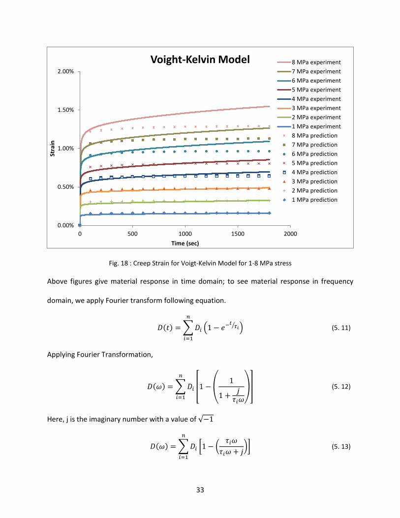
Fig. 18 : Creep Strain for Voigt-Kelvin Model for 1-8 MPa stress

Above figures give material response in time domain; to see material response in frequency

domain, we apply Fourier transform following equation.

𝐷(𝑡) = �𝐷𝑖 �1 − 𝑒−𝑡 𝜏𝑖� �

𝑛

𝑖=1

(5. 11)

Applying Fourier Transformation,

𝐷(𝜔) = �𝐷𝑖

𝑛

𝑖=1

�1 − �1

1 + 𝑗𝜏𝑖𝜔

�� (5. 12)

Here, j is the imaginary number with a value of √−1

𝐷(𝜔) = �𝐷𝑖

𝑛

𝑖=1

�1 − �𝜏𝑖𝜔

𝜏𝑖𝜔 + 𝑗�� (5. 13)

0.00%

0.50%

1.00%

1.50%

2.00%

0 500 1000 1500 2000

Stra

in

Time (sec)

Voight-Kelvin Model 8 MPa experiment7 MPa experiment6 MPa experiment5 MPa experiment4 MPa experiment3 MPa experiment2 MPa experiment1 MPa experiment8 MPa prediction7 MPa prediction6 MPa prediction5 MPa prediction4 MPa prediction3 MPa prediction2 MPa prediction1 MPa prediction

33

Multiply and divide by conjugate

𝐷(𝜔) = �𝐷𝑖

𝑛

𝑖=1

�1 − �𝜏𝑖𝜔

𝜏𝑖𝜔 + 𝑗� �𝜏𝑖𝜔 − 𝑗𝜏𝑖𝜔 − 𝑗

�� (5. 14)

𝐷(𝜔) = �𝐷𝑖 �1 − �𝜏𝑖2𝜔2 − 𝑗𝜏𝑖𝜔𝜏𝑖2𝜔2 − 𝑗2

��𝑛

𝑖=1

(5. 15)

𝐷(𝜔) = �𝐷𝑖 �1 − �𝜏𝑖2𝜔2 − 𝑗𝜏𝑖𝜔𝜏𝑖2𝜔2 + 1

��𝑛

𝑖=1

(5. 16)

𝐷(𝜔) = �𝐷𝑖 �1 + 𝜏𝑖2𝜔2 − 𝜏𝑖2𝜔2 + 𝑗𝜏𝑖𝜔

𝜏𝑖2𝜔2 + 1�

𝑛

𝑖=1

(5. 17)

𝐷(𝜔) = �𝐷𝑖 �1 + 𝑗𝜏𝑖𝜔

1 + 𝜏𝑖2𝜔2�𝑛

𝑖=1

(5. 18)

Separating real and imaginary parts, we get

(𝑆𝑡𝑜𝑟𝑎𝑔𝑒 𝑀𝑜𝑑𝑢𝑙𝑢𝑠) 𝐷′(𝜔) = ��𝐷𝑖

1 + 𝜏𝑖2𝜔2�𝑛

𝑖=1

(5. 19)

(𝐿𝑜𝑠𝑠 𝑀𝑜𝑑𝑢𝑙𝑢𝑠) 𝐷′′(𝜔) = �𝐷𝑖 �𝜏𝑖𝜔

1 + 𝜏𝑖2𝜔2�𝑛

𝑖=1

(5. 20)

5.3 Prony Series

A common form for the linear viscoelastic response is given by Prony Series by the

following equation [10]-[20]:

�𝛼𝑖𝑒−𝑡 𝜏𝑖�

𝑁

𝑖=1

(5. 21)

Here, 𝜏𝑖 are the time constants and 𝛼𝑖 are the exponential coefficients.

For creep test we use the creep compliance equation [10]-[20]

34

Є(𝑡) = 𝐽(𝑡)𝜎0 (5. 22)

Here, 𝐽(𝑡) is the creep compliance function and its response under Prony Series is given by

𝐽(𝑡) = 𝐽0.�1 −�𝑝𝑖𝑒−𝑡 𝜏𝑖�

𝑛

𝑖=1

� (5. 23)

Є(𝑡) = 𝜎0𝐽(𝑡) + � 𝐽(𝑡 − 𝜉)𝑑𝜎(𝜉)𝑑𝜉

𝑑𝜉𝑡

0 (5. 24)

𝜎(𝑡) = �𝜎1𝑡

(𝑡1 − 𝑡0)� ; 𝑡0 < 𝑡 < 𝑡1

𝜎1 ; 𝑡1 < 𝑡 < 𝑡2�

𝑑𝜎𝑑𝑡

= �𝜎1

(𝑡1 − 𝑡0)� ; 𝑡0 < 𝑡 < 𝑡1 0 ; 𝑡1 < 𝑡 < 𝑡2

�

Here, 𝜎0 = 0, 𝜎1 is the stress level at which the stress is kept constant, and 𝑡0 = 0

Step 1(𝒕𝟎 < 𝒕 ≤ 𝒕𝟏)

Є1(𝑡) = 𝜎0𝐽(𝑡) + � 𝐽(𝑡 − 𝜉)𝑑𝜎(𝜉)𝑑𝜉

𝑑𝜉𝑡

0 (5. 25)

Є1(𝑡) = 𝐽0𝜎1𝑡1

�𝑡 −�𝑝𝑖𝜏𝑖 +�𝑝𝑖𝜏𝑖𝑒−𝑡 𝜏𝑖� � (5. 26)

Є1(𝑡) = 𝐽0𝜎1𝑡1

�𝑡 − 𝑃1𝜏1 − 𝑃2𝜏2 + 𝑃1𝜏1𝑒−𝑡 𝜏1� + 𝑃2𝜏2𝑒

−𝑡 𝜏2� � (5. 27)

We obtained a two-term Prony Series

Step 2(𝒕𝟏 < 𝒕 ≤ 𝒕𝟐)

In this step, the stress is kept constant.

Є2(𝑡) = 𝐽0𝜎1𝑡1

�𝑡1 −�𝑝𝑖𝜏𝑖𝑒−(𝑡−𝑡1)

𝜏𝑖� + �𝑝𝑖𝜏𝑖𝑒−𝑡 𝜏𝑖� � (5. 28)

Є2(𝑡) = 𝐽0𝜎1𝑡1

�𝑡1 − 𝑃1𝜏1𝑒−(𝑡−𝑡1)

𝜏1� − 𝑃2𝜏2𝑒−(𝑡−𝑡1)

𝜏2� + 𝑃1𝜏1𝑒−𝑡 𝜏1� + 𝑃2𝜏2𝑒

−𝑡 𝜏2� � (5. 29)

35

We used the following material parameters to predict our creep response

Table 6 : Creep Material Parameters for Prony Series

𝐽 1.75 × 10−9

𝑃1 0.12

𝑃2 0.2

𝜏1 25

𝜏2 1000

Fig. 19 gives creep strain prediction using Prony Series. We can see that it gives a perfect

response till 5 MPa stress, and at higher stress levels it does not show a good response. It gives

better response than previous two viscoelastic models as it catches the trend of the creep

strain and shows a better fit.

Fig. 19: Creep Strain prediction for Prony Series

0.00%

0.50%

1.00%

1.50%

2.00%

2.50%

0 500 1000 1500 2000

Cree

p St

rain

Time (sec)

Prony Series 10 MPa9 MPa8 MPa7 MPa6 MPa5 MPa4 MPa3 MPa2 MPa1 MPa10 MPa prediction9 MPa prediction8 MPa prediction7 MPa prediction6 MPa prediction5 MPa prediction4 MPa prediction3 MPa prediction2 MPa prediction1 MPa prediction

36

To get material response in frequency domain for Prony Series, we apply Fourier

transformation. Prony Series is represented in terms of shear relaxation modulus by the

following expression [20]:

𝑔𝑅(𝑡) = 1 −�𝑔𝑖 �1 − 𝑒−𝑡 𝜏𝑖� �

𝑁

𝑖=1

(5. 30)

Here, 𝑔𝑖 and 𝜏𝑖 are material parameters and 𝑔𝑅(𝑡) is the dimensionless relaxation modulus

given by

𝑔𝑅(𝑡) =𝐺𝑅(𝑡)𝐺0

(5. 31)

𝐺𝑅(𝑡)𝐺0

= 1 −�𝑔𝑖 �1 − 𝑒−𝑡 𝜏𝑖� �

𝑁

𝑖=1

(5. 32)

𝐺𝑅(𝑡)𝐺0

= 1 −�𝑔𝑖

𝑁

𝑖=1

+ �𝑔𝑖

𝑁

𝑖=1

𝑒−𝑡 𝜏𝑖� (5. 33)

𝐺𝑅(𝑡) = 𝐺0 �1 −�𝑔𝑖

𝑁

𝑖=1

+ �𝑔𝑖

𝑁

𝑖=1

𝑒−𝑡 𝜏𝑖� � (5. 34)

𝐺𝑅(𝑡) = 𝐺0 �1 −�𝑔𝑖

𝑁

𝑖=1

� + 𝐺0�𝑔𝑖

𝑁

𝑖=1

𝑒−𝑡 𝜏𝑖� (5. 35)

Apply Fourier Transformation:

𝐺(𝜔) = 𝐺0 �1 −�𝑔𝑖

𝑁

𝑖=1

� + 𝐺0�𝑔𝑖

𝑁

𝑖=1

1

1 + 𝑗𝜏𝑖𝜔�

(5. 36)

Here, j is the imaginary number with a value of √−1

37

𝐺(𝜔) = 𝐺0 �1 −�𝑔𝑖

𝑁

𝑖=1

� + 𝐺0�𝑔𝑖

𝑁

𝑖=1

1

1 + 𝑗𝜏𝑖𝜔�

(5. 37)

𝐺(𝜔) = 𝐺0 �1 −�𝑔𝑖

𝑁

𝑖=1

� + 𝐺0�𝑔𝑖

𝑁

𝑖=1

𝜏𝑖𝜔𝜏𝑖𝜔 + 𝑗

(5. 38)

Multiply and divide by conjugate:

𝐺(𝜔) = 𝐺0 �1 −�𝑔𝑖

𝑁

𝑖=1

� + 𝐺0�𝑔𝑖

𝑁

𝑖=1

�𝜏𝑖𝜔

𝜏𝑖𝜔 + 𝑗� �𝜏𝑖𝜔 − 𝑗𝜏𝑖𝜔 − 𝑗

� (5. 39)

𝐺(𝜔) = 𝐺0 �1 −�𝑔𝑖

𝑁

𝑖=1

� + 𝐺0�𝑔𝑖

𝑁

𝑖=1

�𝜏𝑖2𝜔2 − 𝜏𝑖𝜔𝑗𝜏𝑖2𝜔2 − 𝑗2

� (5. 40)

𝐺(𝜔) = 𝐺0 �1 −�𝑔𝑖

𝑁

𝑖=1

� + 𝐺0�𝑔𝑖

𝑁

𝑖=1

�𝜏𝑖2𝜔2

𝜏𝑖2𝜔2 + 1� − 𝑗𝐺0�𝑔𝑖

𝑁

𝑖=1

�𝜏𝑖𝜔

𝜏𝑖2𝜔2 + 1� (5. 41)

We know that

𝐺(𝜔) = 𝐺′(𝜔) + 𝑗𝐺′′(𝜔) (5. 42)

Separating real and imaginary parts, we get

(𝑆𝑡𝑜𝑟𝑎𝑔𝑒 𝑀𝑜𝑑𝑢𝑙𝑢𝑠) 𝐺′(𝜔) = 𝐺0 �1 −�𝑔𝑖

𝑁

𝑖=1

� + 𝐺0�𝑔𝑖

𝑁

𝑖=1

�𝜏𝑖2𝜔2

1 + 𝜏𝑖2𝜔2� (5. 43)

(𝐿𝑜𝑠𝑠 𝑀𝑜𝑑𝑢𝑙𝑢𝑠) 𝐺′′(𝜔) = 𝐺0�𝑔𝑖

𝑁

𝑖=1

�𝜏𝑖𝜔

1 + 𝜏𝑖2𝜔2� (5. 44)

38

CHAPTER 6

NON-LINEAR VISCOELASTIC MODEL

In this chapter we will discuss methods of characterization non-linear viscoelastic

materials. We will be using constitutive equations from Chapter 1 and using experimental data

(creep test data) to obtain material parameters. In small deformation materials, the total strain

is the sum of viscoelastic strain and viscoplastic strain [14]-[19].

Є(𝑡) = Є𝑣𝑒(𝑡) + Є𝑣𝑝(𝑡) (6. 1)

While, the incremental strain is given by

𝛥Є(𝑡) = 𝛥Є𝑣𝑒(𝑡) + 𝛥Є𝑣𝑝(𝑡) At time t>0 (6. 2)

Here, Є𝑣𝑒refers to viscoelastic strain and Є𝑣𝑝 refers to viscoplastic strain and 𝛥Є𝑣𝑒 gives the

incremental viscoelastic strain while 𝛥Є𝑣𝑝 gives the incremental viscoplastic strain. In our

model we are only concerned with elastic deformation and have omitted the viscoplastic part.

Schapery equation in 1-D form is given by the following equation [14]-[19],

Є(𝑡) = 𝑔0𝐷0𝜎 + 𝑔1 � 𝛥𝐷[𝜓(𝑡) − 𝜓′(𝜏)]𝑡

0

𝑑𝑔2𝜎𝑑𝜏

𝑑𝜏 (1) (6. 3)

Here, 𝐷0 and 𝛥𝐷(𝜓) are the instantaneous and transient linear viscoelastic creep compliance

components which have been defined previously, and 𝜓 is reduced-time given by

𝜓 = �𝑑𝑡′

𝑎𝜎[𝜎(𝑡′)]

𝑡

0

(6. 4)

And

𝜓′ = 𝜓(𝜏) = �𝑑𝑡′

𝑎𝜎[𝜎(𝑡′)]

𝜏

0

(6. 5)

39

In a 3-D representation of Schapery model, stress and strain are given by its deviatoric and

hydrostatic components.

𝑆𝑖𝑗 = 𝜎𝑖𝑗 −13𝛿𝑖𝑗𝜎𝑘𝑘 (6. 6)

𝑑𝑖𝑗 = Є𝑖𝑗 −13𝛿𝑖𝑗Є𝑘𝑘 (6. 7)

Here, 𝛿𝑖𝑗 is Kronecker Delta and 13𝜎𝑘𝑘 and 1

3Є𝑘𝑘 are the hydrostatic stress and strain

respectively.

For an isotropic linear elastic material, the relation between stress and strain can be expressed

as [14]-[19]

Є𝑖𝑗 =12𝐽𝑆𝑖𝑗 +

19𝐵𝛿𝑖𝑗𝜎𝑘𝑘 (6. 8)

Here, 𝐽 is the shear compliance and 𝐵 is the bulk compliance.

So, using our 1-D Schapery equation, we can get 3-D non-linear viscoelastic model as

Є𝑖𝑗(𝑡) =12𝑔0𝐽0𝑆𝑖𝑗(𝑡) +

12𝑔1 � 𝛥𝐽[𝜓(𝑡) − 𝜓′(𝜏)]

𝑡

0

𝑑𝑔2𝑆𝑖𝑗𝑑𝜏

𝑑𝜏

+19𝑔0𝐵0𝛿𝑖𝑗𝜎𝑘𝑘(𝑡) +

19𝑔1𝛿𝑖𝑗 � 𝛥𝐵[𝜓(𝑡) − 𝜓′(𝜏)]

𝑡

0

𝑑𝑔2𝜎𝑘𝑘𝑑𝜏

𝑑𝜏

(6. 9)

The instantaneous shear compliance 𝐽0 and instantaneous bulk compliance 𝐵0 can be given by

the following equations, where ν is the Poison’s ratio [14]-[19].

𝐽0 = 2(1 + 𝝂)𝛥𝐷(𝜓) (6. 10)

𝐵0 = 3(1 − 2𝝂)𝛥𝐷(𝜓) (6. 11)

The transient tensile component 𝛥𝐷(𝜓) is expressed in terms of Prony series [17]

40

𝛥𝐷(𝜓) = �𝐷𝑛[1 − exp (−𝜆𝑛𝜓)]𝑁

1

(6. 12)

Here, 𝐷𝑛 and 𝜆𝑛 are Prony constants which can be determined by tensile creep compliance

data.

Using the relation between shear compliance and tensile compliance we can write the following

equation as;

𝛥𝐽(𝜓) = �𝐽𝑛[1 − exp(−𝜆𝑛𝜓)]𝑁

1

(6. 13)

Similarly,

𝛥𝐵(𝜓) = �𝐵𝑛[1 − exp(−𝜆𝑛𝜓)]𝑁

1

(6. 14)

Here,

𝐽𝑛 = 2(1 + 𝝂)𝐷𝑛 (6. 15)

𝐵 = 3(1 − 2𝝂)𝐷𝑛 (6. 16)

The Prony constants 𝐷𝑛 and 𝜆𝑛 can be obtained creep test data by using curve fitting

approach, and by using the relation between shear compliance and tensile compliance we can

obtain the remaining terms. At first linear response of the material is considered (at low value

of stress) and non-linear material parameters 𝑔0,𝑔1,𝑔2, and 𝑎𝜎 is considered as 1.

Transient creep compliance can be given by the following by using simple power law [17]-[19]

𝛥𝐷(𝜓) = 𝐶𝜓𝑚𝑚 (6. 17)

Here, 𝐶 and 𝑚 are material constants. In the case of creep test where σ is held constant for

time> 0, equation (6. 3 becomes

41

Є𝑐(𝑡) = 𝑔0𝐷0𝜎 +𝑔1𝑔2𝐶𝑎𝜎𝑚𝑚

𝑡𝑚𝑚 (6. 18)

Taking low stress region into account, in our case creep test at 1 MPa, where the response of

the material is almost linear and non-linear material parameters 𝑔0,𝑔1,𝑔2, and 𝑎𝜎 is

considered as 1, above equation deduced into [17][19]

Є𝑐(𝑡) = 𝐷0𝜎 + 𝐶𝑡𝑚𝑚 (6. 19)

Using curve fitting technique to find out the constants 𝐷0, 𝐶 and 𝑚. Using the above

equations, creep strain response is predicted by using the following equation.

Є𝑐(𝑡) = �𝑔0𝐷0 + 𝑔1𝑔2𝛥𝐷�𝑡 𝑎𝜎� �� 𝜎 (6. 20)

This is the required equation we will be using in order to predict our response. We use the

following material parameters to get the response, while 𝑔0,𝑔1,𝑔2,𝑎𝜎 = 1 is used for linear

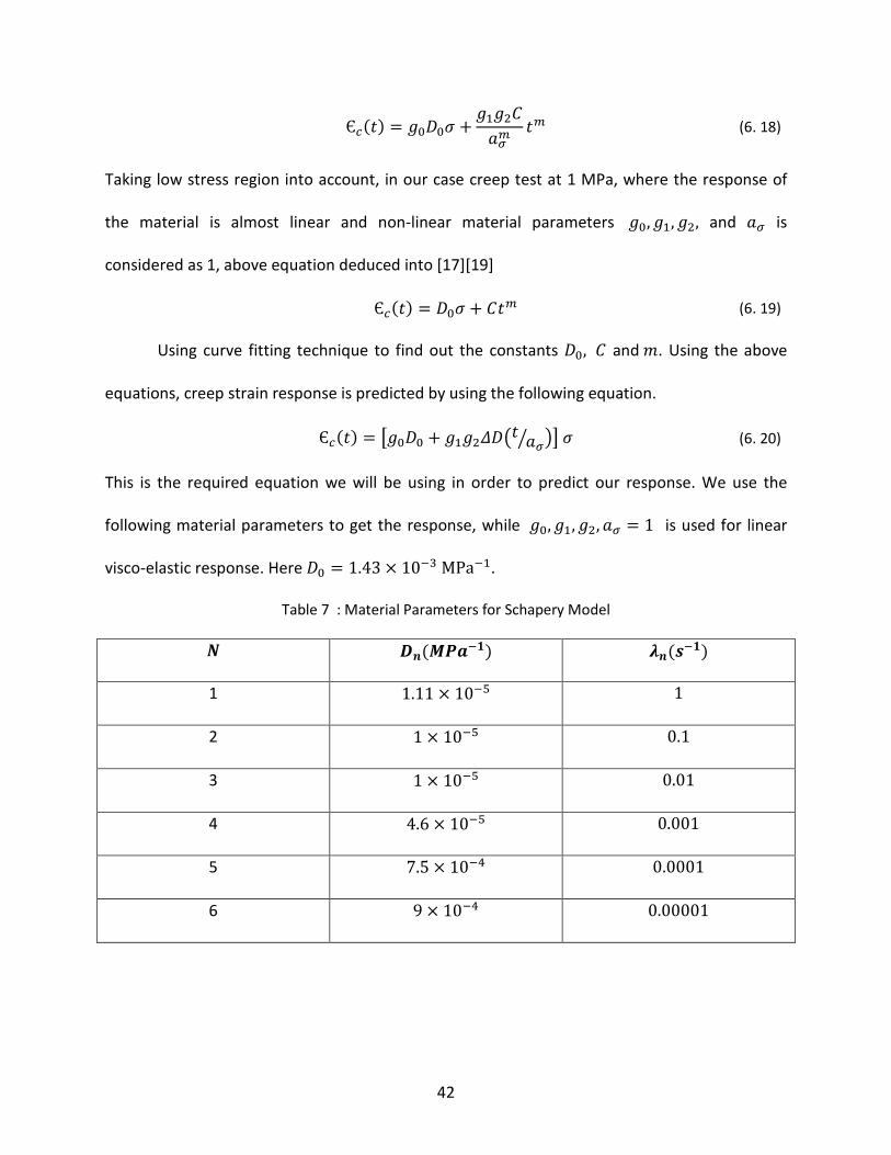
visco-elastic response. Here 𝐷0 = 1.43 × 10−3 MPa−1.

Table 7 : Material Parameters for Schapery Model

𝑵 𝑫𝒏(𝑴𝑷𝒂−𝟏) 𝝀𝒏(𝒔−𝟏)

1 1.11 × 10−5 1

2 1 × 10−5 0.1

3 1 × 10−5 0.01

4 4.6 × 10−5 0.001

5 7.5 × 10−4 0.0001

6 9 × 10−4 0.00001

42

Fig. 20 : Schapery Model Prediction of Creep Test

Fig. 20 gives creep strain prediction of Procast using Schapery model. We can see that it gives a

better material response than Prony series, even at higher stress values.

Fig. 21 : Nonlinear Parameters for Schapery Model at Various Stress Levels

0.00%

0.50%

1.00%

1.50%

2.00%

2.50%

0 500 1000 1500 2000

Cree

p St

rain

Time (sec)

Schapery Model 10 MPa9 MPa8 MPa7 MPa6 MPa5 MPa4 MPa3 MPa2 MPa1 MPa10 MPa prediction9 MPa prediction8 MPa prediction7 MPa Prediction6 MPa Prediction5 MPa Prediction4 MPa prediction3 MPa Prediction2MPa Prediction1MPa Prediction

0.5

1.5

0 1 2 3 4 5 6 7 8 9 10 11 12

Non

linea

r vis

coel

astic

par

amet

ers

Stress (MPa)

g0

g1

g2

a

43

Nonlinear viscoelastic parameters can be obtained for other stress levels by using the constants

listed in Table 8 for polynomial equations, where subscript of α denotes exponent of stress for

example;

𝑓(𝑔0,𝑔1,𝑔2,𝑎) = 𝛼𝑛𝜎𝑛 + 𝛼𝑛−1𝜎𝑛−1 + ⋯+ 𝛼0𝜎0

Table 8 : Polynomial Constants for Nonlinear Material Paramters

𝜶𝟒 𝜶𝟑 𝜶𝟐 𝜶𝟏 𝜶𝟎

𝑔0 - - 0.0032 -0.0111 1.0037

𝑔1 0.0005 -0.0107 0.0719 -0.1091 1.0119

𝑔2 0.0004 -0.0085 0.057 -0.0866 1.0095

𝑎 0.0001 -0.0026 0.0171 -0.0254 1.0026

Equation (6. 20 gives material response in time domain, to obtain material response in

frequency domain we apply Fourier transformation.

Є𝑐(𝑡)𝜎

= �𝑔0𝐷0 + 𝑔1𝑔2𝛥𝐷�𝑡 𝑎𝜎� �� (6. 21)

Using equation (6. 12, we get

𝐷(𝑡) = 𝑔0𝐷0 + 𝑔1𝑔2�𝐷𝑛�1 − exp �−𝜆𝑛 𝑡 𝑎𝜎� ��𝑁

1

(6. 22)

Applying Fourier Transformation,

𝐷(𝜔) = 𝑔0𝐷0 + 𝑔1𝑔2𝐷𝑛 �1 − �1

1 + 𝑗𝜔 �

𝜆𝑛𝑎 �

�� (6. 23)

44

𝐷(𝜔) = 𝑔0𝐷0 + 𝑔1𝑔2𝐷𝑛 �1 − �𝜔

𝜔 + 𝑗 �𝜆𝑛𝑎 ��� (6. 24)

Multiply and divide by conjugate

𝐷(𝜔) = 𝑔0𝐷0 + 𝑔1𝑔2𝐷𝑛 �1 − �𝜔

𝜔 + 𝑗 �𝜆𝑛𝑎 ���

𝜔 − 𝑗 �𝜆𝑛𝑎 �

𝜔 − 𝑗 �𝜆𝑛𝑎 ��� (6. 25)

𝐷(𝜔) = 𝑔0𝐷0 + 𝑔1𝑔2𝐷𝑛

⎣⎢⎢⎡1 −

⎝

⎛𝜔2 − 𝑗𝜔 �𝜆𝑛𝑎 �

𝜔2 + �𝜆𝑛𝑎 �2

⎠

⎞

⎦⎥⎥⎤ (6. 26)

𝐷(𝜔) = 𝑔0𝐷0 + 𝑔1𝑔2𝐷𝑛

⎝

⎛𝜔2 + �𝜆𝑛𝑎 �

2− 𝜔2 + 𝑗𝜔 �𝜆𝑛𝑎 �

𝜔2 + �𝜆𝑛𝑎 �2

⎠

⎞ (6. 27)

𝐷(𝜔) = 𝑔0𝐷0 + 𝑔1𝑔2𝐷𝑛

⎝

⎛�𝜆𝑛𝑎 �

2+ 𝑗𝜔 �𝜆𝑛𝑎 �

𝜔2 + �𝜆𝑛𝑎 �2

⎠

⎞ (6. 28)

Separating real and imaginary parts, we get

(𝑆𝑡𝑜𝑟𝑎𝑔𝑒 𝑀𝑜𝑑𝑢𝑙𝑢𝑠) 𝐷′(𝜔) = 𝑔0𝐷0 + 𝑔1𝑔2𝐷𝑛

⎝

⎛�𝜆𝑛𝑎 �

2

𝜔2 + �𝜆𝑛𝑎 �2

⎠

⎞ (6. 29)

(𝐿𝑜𝑠𝑠 𝑀𝑜𝑑𝑢𝑙𝑢𝑠) 𝐷′(𝜔) = 𝑔1𝑔2𝐷𝑛

⎝

⎛𝜔 �𝜆𝑛𝑎 �

𝜔2 + �𝜆𝑛𝑎 �2

⎠

⎞ (6. 30)

45

CHAPTER 7

VALIDATION OF MODEL

In this chapter we will try to validate our models with the uniaxial tensile tests we

performed. For this purpose we have taken tensile test data in Fig. 8 and plotted its response

for various models. We have considered only the elastic region which in our case is under 2.5%

strain, which can be seen by following figure.

Fig. 22 : Strain-Rate Dependent Tensile Test Data Including Yielding Region

The yielding region is considered to be under 2.5 % strain. This is due to the fact that we are

considering the elastic response, rather than the plastic deformation. We will try to fit the

validation of different material model under 2.5 % strain.

0

10

20

30

40

50

60

0.00% 5.00% 10.00% 15.00% 20.00%

Stre

ss (M

Pa)

Strain (%)

Stress-Strain

Strain Rate = 0.001

Strain Rate = 0.005

Strain Rate = 0.01

Strain Rate = 0.05

Yield Point

46

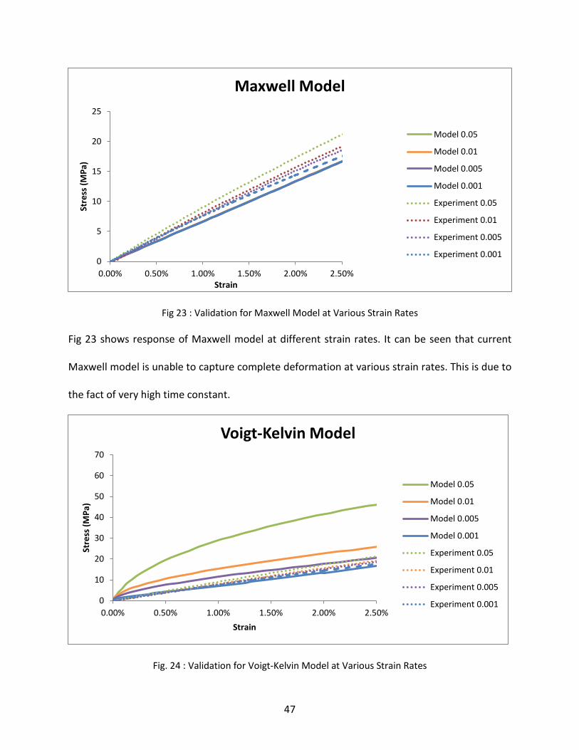
Fig 23 : Validation for Maxwell Model at Various Strain Rates

Fig 23 shows response of Maxwell model at different strain rates. It can be seen that current

Maxwell model is unable to capture complete deformation at various strain rates. This is due to

the fact of very high time constant.

Fig. 24 : Validation for Voigt-Kelvin Model at Various Strain Rates

0

5

10

15

20

25

0.00% 0.50% 1.00% 1.50% 2.00% 2.50%

Stre

ss (M

Pa)

Strain

Maxwell Model

Model 0.05

Model 0.01

Model 0.005

Model 0.001

Experiment 0.05

Experiment 0.01

Experiment 0.005

Experiment 0.001

0

10

20

30

40

50

60

70

0.00% 0.50% 1.00% 1.50% 2.00% 2.50%

Stre

ss (M

Pa)

Strain

Voigt-Kelvin Model

Model 0.05

Model 0.01

Model 0.005

Model 0.001

Experiment 0.05

Experiment 0.01

Experiment 0.005

Experiment 0.001

47

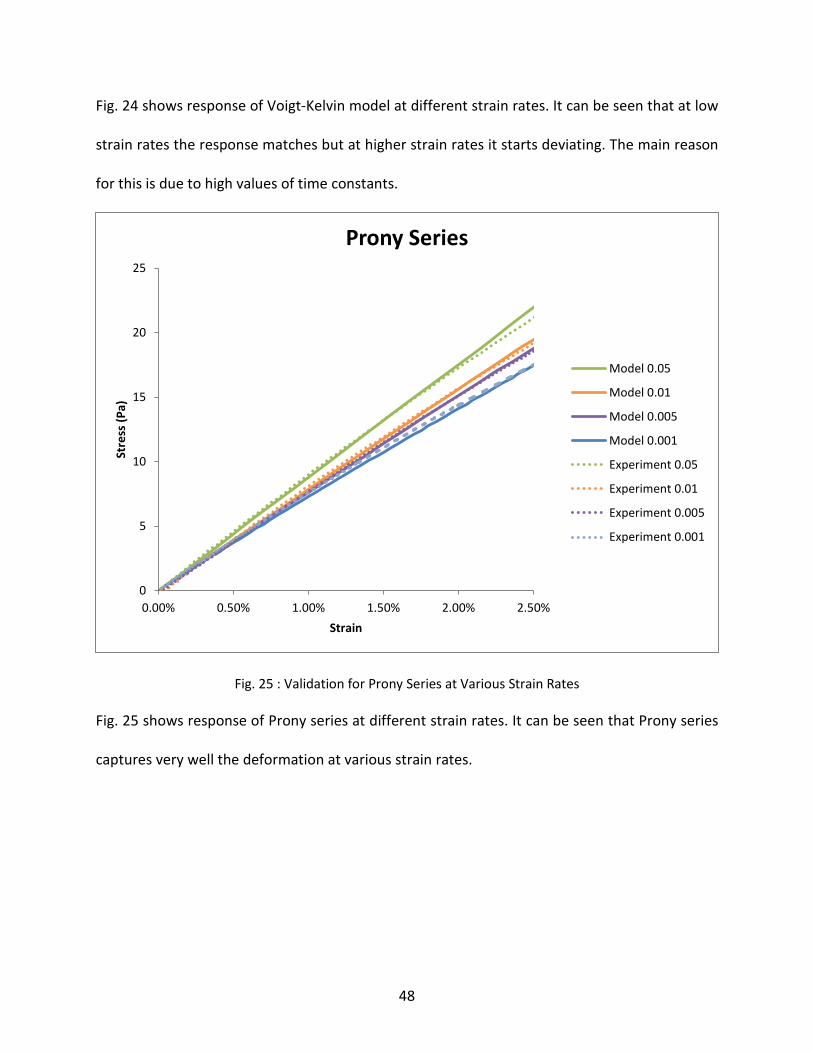
Fig. 24 shows response of Voigt-Kelvin model at different strain rates. It can be seen that at low

strain rates the response matches but at higher strain rates it starts deviating. The main reason

for this is due to high values of time constants.

Fig. 25 : Validation for Prony Series at Various Strain Rates

Fig. 25 shows response of Prony series at different strain rates. It can be seen that Prony series

captures very well the deformation at various strain rates.

0

5

10

15

20

25

0.00% 0.50% 1.00% 1.50% 2.00% 2.50%

Stre

ss (P

a)

Strain

Prony Series

Model 0.05

Model 0.01

Model 0.005

Model 0.001

Experiment 0.05

Experiment 0.01

Experiment 0.005

Experiment 0.001

48

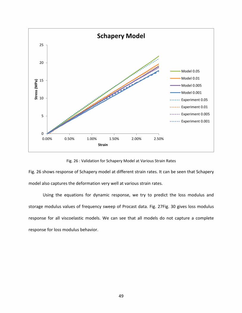
Fig. 26 : Validation for Schapery Model at Various Strain Rates

Fig. 26 shows response of Schapery model at different strain rates. It can be seen that Schapery

model also captures the deformation very well at various strain rates.

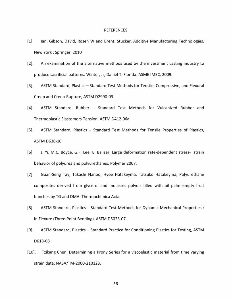
Using the equations for dynamic response, we try to predict the loss modulus and

storage modulus values of frequency sweep of Procast data. Fig. 27Fig. 30 gives loss modulus

response for all viscoelastic models. We can see that all models do not capture a complete

response for loss modulus behavior.

0

5

10

15

20

25

0.00% 0.50% 1.00% 1.50% 2.00% 2.50%

Stre

ss (M

Pa)

Strain

Schapery Model

Model 0.05

Model 0.01

Model 0.005

Model 0.001

Experiment 0.05

Experiment 0.01

Experiment 0.005

Experiment 0.001

49

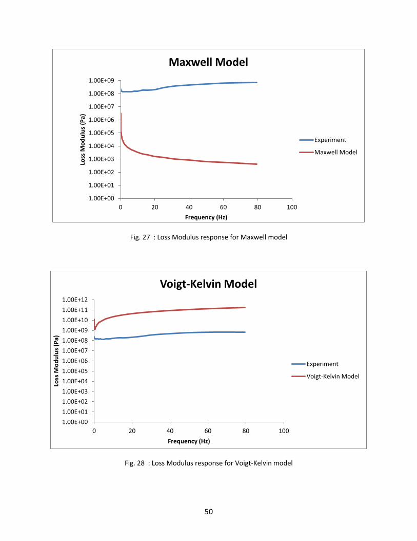
Fig. 27 : Loss Modulus response for Maxwell model

Fig. 28 : Loss Modulus response for Voigt-Kelvin model

1.00E+00

1.00E+01

1.00E+02

1.00E+03

1.00E+04

1.00E+05

1.00E+06

1.00E+07

1.00E+08

1.00E+09

0 20 40 60 80 100

Loss

Mod

ulus

(Pa)

Frequency (Hz)

Maxwell Model

Experiment

Maxwell Model

1.00E+001.00E+011.00E+021.00E+031.00E+041.00E+051.00E+061.00E+071.00E+081.00E+091.00E+101.00E+111.00E+12

0 20 40 60 80 100

Loss

Mod

ulus

(Pa)

Frequency (Hz)

Voigt-Kelvin Model

Experiment

Voigt-Kelvin Model

50

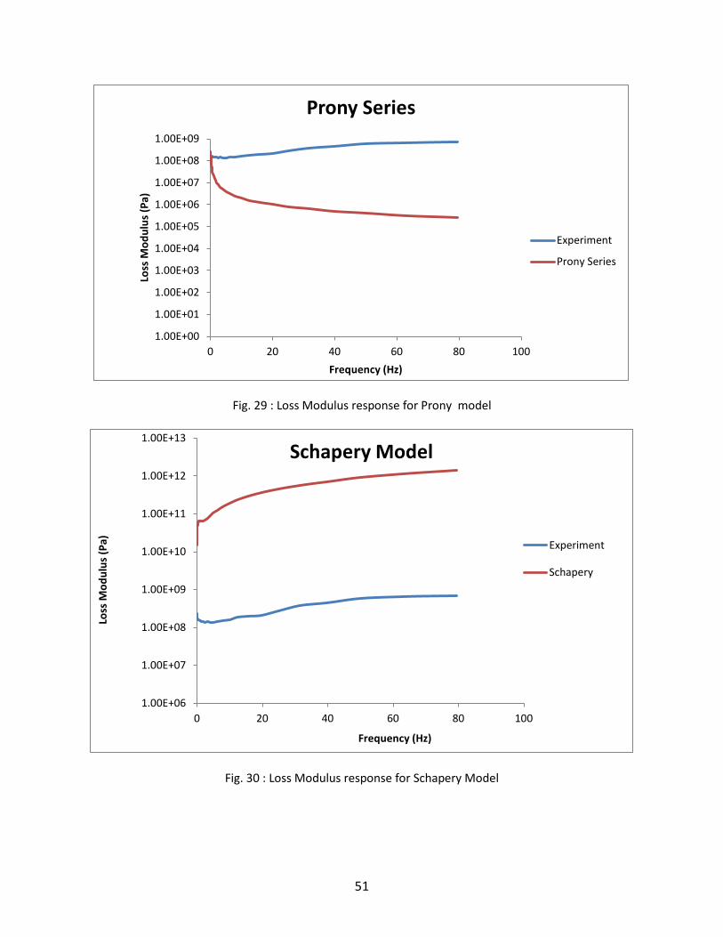
Fig. 29 : Loss Modulus response for Prony model

Fig. 30 : Loss Modulus response for Schapery Model

1.00E+00

1.00E+01

1.00E+02

1.00E+03

1.00E+04

1.00E+05

1.00E+06

1.00E+07

1.00E+08

1.00E+09

0 20 40 60 80 100

Loss

Mod

ulus

(Pa)

Frequency (Hz)

Prony Series

Experiment

Prony Series

1.00E+06

1.00E+07

1.00E+08

1.00E+09

1.00E+10

1.00E+11

1.00E+12

1.00E+13

0 20 40 60 80 100

Loss

Mod

ulus

(Pa)

Frequency (Hz)

Schapery Model

Experiment

Schapery

51

Using the equations for dynamic response (storage modulus), we try to predict the

storage modulus values of frequency sweep of Procast data. Fig. 30 Fig. 31Fig. 34 gives storage

modulus response for all viscoelastic models. We can see that Maxwell and Voigt-Kelvin models

do not capture the complete dynamic response while Prony series and Schapery model gives a

better prediction in terms of storage modulus.

Fig. 31 : Storage Modulus response for Maxwell model

1.00E+00

1.00E+01

1.00E+02

1.00E+03

1.00E+04

1.00E+05

1.00E+06

1.00E+07

1.00E+08

1.00E+09

1.00E+10

1.00E+11

1.00E+12

0 20 40 60 80 100

Stor

age

Mod

ulus

(Pa)

Frequency (Hz)

Maxwell Model

Experiment

Maxwell Model

52

Fig. 32 : Storage Modulus response for Voigt-Kelvin model

Fig. 33 : Storage Modulus response for Prony Series

1.00E+00

1.00E+02

1.00E+04

1.00E+06

1.00E+08

1.00E+10

1.00E+12

1.00E+14

0 20 40 60 80 100

Stor

age

Mod

ulus

(Pa)

Frequency (Hz)

Voigt-Kelvin Model

Experiment

Voigt-Kelvin

1.00E+06

1.00E+07

1.00E+08

1.00E+09

1.00E+10

0 20 40 60 80 100

Stor

age

Mod

ulus

(Pa)

Frequency (Hz)

Prony Series

Experiment

Prony Series

53

Fig. 34 : Storage Modulus response for Schapery model

1.00E+06

1.00E+07

1.00E+08

1.00E+09

1.00E+10

0 20 40 60 80 100

Stor

age

Mod

ulus

(Pa)

Frequency (Hz)

Schapery Model

Experiment Schapery

54

CHAPTER 8

CONCLUSIONS AND FUTURE WORK

Additive manufacturing is a relatively new technique and mechanical response of the base

material used for printing is also unknown. In my thesis I have conducted various tests to

determine the base properties for Procast material. My major findings include

(i) Glass transition temperature of Procast, which is in the range of 81°C

(ii) Melting temperature of Procast which is around 337.1°C

(iii) Density of Procast material can be seen from Table 3 which is around 1125-1162

kg/m3

(iv) Strain rate dependent elastic modulus which can be seen from Table 2 which is

around 0.7-0.8 GPa

(v) Procast yield stress which is around 16-19 MPa

(vi) Linear viscoelastic stress level for Procast which is around 3 MPa

(vii) Prony Series and Schapery Model show good validation response at various strain

rates.

These finding from my thesis can benefit the research community. It can also be seen from my

viscoelastic models that Prony Series show better fit for linear viscoelastic response and

Schapery model shows good fit for all stress levels for non-linear viscoelastic region.

So far, I have studied the material response for Procast material, in the future we can also look

at complex cellular geometry behavior of Procast material.

55

REFERENCES

[1]. Ian, Gibson, David, Rosen W and Brent, Stucker. Additive Manufacturing Technologies.

New York : Springer, 2010

[2]. An examination of the alternative methods used by the investment casting industry to

produce sacrificial patterns. Winter, Jr, Daniel T. Florida: ASME IMEC, 2009.

[3]. ASTM Standard, Plastics – Standard Test Methods for Tensile, Compressive, and Flexural

Creep and Creep-Rupture, ASTM D2990-09

[4]. ASTM Standard, Rubber – Standard Test Methods for Vulcanized Rubber and

Thermoplastic Elastomers-Tension, ASTM D412-06a

[5]. ASTM Standard, Plastics – Standard Test Methods for Tensile Properties of Plastics,

ASTM D638-10

[6]. J. Yi, M.C. Boyce, G.F. Lee, E. Balizer, Large deformation rate-dependent stress- strain

behavior of polyurea and polyurethanes: Polymer 2007.

[7]. Guan-Seng Tay, Takashi Nanbo, Hyoe Hatakeyma, Tatsuko Hatakeyma, Polyurethane

composites derived from glycerol and molasses polyols filled with oil palm empty fruit

bunches by TG and DMA: Thermochimica Acta.

[8]. ASTM Standard, Plastics – Standard Test Methods for Dynamic Mechanical Properties :

In Flexure (Three-Point Bending), ASTM D5023-07

[9]. ASTM Standard, Plastics – Standard Practice for Conditioning Plastics for Testing, ASTM

D618-08

[10]. Tzikang Chen, Determining a Prony Series for a viscoelastic material from time varying

strain data: NASA/TM-2000-210123.

56

[11]. Montgomery T. Shaw, William J. MacKnight, Introduction to Polymer Viscoelasticity, 3rd

Edition, Chapter 3 Viscoelastic Models.

[12]. J.D. Ferry, Viscoelastic Properties of Polymers, 3rd ed., Wiley, New York, 1980

[13]. Ian M. Ward, John Sweeney, Mechanical Properties of Solid Polymers, 3rd Ed.

[14]. D. Gamby, L. Blugeon, On the characterization by Schapery’s model of non-linear

viscoelastic materials

[15]. J. Lai, A. Bakker, An integral constitutive equation for nonlinear plasto-viscoelastic

behavior of high-density Polyethlene

[16]. Jeong Sik Kim, Anastasia H. Muliana, A time- integration method for the viscoelstic-

viscoplastic analysis of polymers and finite element implementation

[17]. Henriksen M. Nonlinear viscoelastic stress analysis-a finite element approach.

Computers and Structures 1984

[18]. Schapery RA. On the characterization of nonlinear viscoelastic materials. Polymer

Engineering and Science 1969

[19]. J. Lai, A. Bakker, 3-D Schapery representation for non-linear viscoelasticity and finite

element implementation

[20]. ABAQUS/Standard User’s Manual, Hibbitt, Karlsson and Sorenson, Inc 1998

[21]. Yong-Rak Kim, Hoki Ban, Soohyok Im, Impact of Truck Loading on Design and Analysis of

Asphaltic Pavement Structures-Phase II

[22]. W.P Bowen, J.C. Jerman, Nonlinear regression using spreadsheets, TiPS 16 (1995)

[23]. L.S. Lasdon, A.D. Waren, A. Jain, M. Ratner, Design and testing of a generalized reduced

gradient code for nonlinear programming, ACM Trans. Mathematical Software 4(1978)

57

[24]. S. Smith, L. Lasdon, Solving large sparse nonlinear programming using GRG, ORSA J.

Comput. 4 (1992)

[25]. Angus M. Brown, A step-by-step guide to non-linear regression analysis of experimental

data using a Microsoft Excel spreadsheet

58