characterization of the formation of filter paper...

Submitted to Image Anal Stereol, 11 pagesOriginal Research Paper

CHARACTERIZATION OF THE FORMATION OF FILTER PAPER USINGTHE BARTLETT SPECTRUM OF THE FIBER STRUCTURE

MARTIN LEHMANN1, JOBST EISENGRABER-PABST2, JOACHIM OHSER3 AND ALIMOGHISEH4

1MANN+HUMMEL GMBH, Hindenburgstr. 45, D-71638 Ludwigsburg, Germany,[email protected], 2MANN+HUMMEL GMBH, Hindenburgstr. 45, D-71638Ludwigsburg, Germany,[email protected], 3Univ. Appl. Sci.Darmstadt, Dept. Math & Nat. Sci., Schofferstr. 3, D-64295Darmstadt, Germany,[email protected], 4Univ. Appl.Sci. Darmstadt, Dept. Math & Nat. Sci., Schofferstr. 3, D-64295 Darmstadt, Germany,[email protected](Submitted)

ABSTRACT

The formation index of filter paper is one of the most important characteristics used in industrial qualitycontrol. Its estimation is often based on subjective comparison chart rating or, even more objective, on thepower spectrum of the paper structure observed on a transmission light table. It is shown that paper formationcan be modeled as Gaussian random fields with a well defined class of correlation functions, and a formationindex can be derived from the density of the Bartlett spectrum estimated from image data. More precisely, theformation index is the mean of the Bessel transform of the correlation taken for wave lengths between 2 and5 mm.

Keywords: Image analysis, fiber systems, filter paper, formation, chart cloudiness, second order characteristics,Bartlett spectrum.

INTRODUCTION

Filter papers are used in a wide variety of fields,ranging from air to oil filters, see Durstet al. (2007).They consist of bounded fibers which are more orless randomly distributed. Except the specific paperweight (i. e. the weight per unit area, also called thenominal grammage), the weight distribution is a veryimportant characteristic of paper. It influences manyproperties of filter papers such as flow rate, particlecollection, efficiency, wet strength, porosity and dustholding capability. Thus, the characterization of theweight distribution is important for industrial qualitycontrol as well as for the development of new filtermaterials and technologies of manufacture.

It is easy to get an impression of the weightdistribution when holding a sheet of paper upagainst light and observing the distribution of theoptical density, known as the paper formation, chartcloudiness or flocculation. Assuming a constantabsorption coefficient for the solid constituents of thepaper structure, the local intensity of the transmittedlight can be related to the local weight density byLambert-Beer’s law. As a consequence there is a closerelationship between weight distribution and formationand, in fact, often one does not distinguish betweenboth. See Van den Akker (1949); McDonaldet al.(1986); Lien and Liu (2006) for the computation ofthe grammage from the absorption of visible light.

The use of soft X-radiation is suggested in Farrington(1988), and the influence of the choice of radiation onthe transmittance is investigated for nonwoven fabricsin Boeckerman (1992) and for paper in Norman andWahren (1976); Bergeronet al. (1988).

Usually, the formation is experimentallydetermined based on two-dimensional (2D) imagesof the paper structure. A transmission light table isused in order to ensure a homogeneous illuminationand the images are acquired by a CCD-camera havinga linear transfer function, such that the pixel valuescan be assumed to be approximately proportional tothe corresponding local intensities. In the simplestcase, a paper structure inspection can be based onsubjective comparison chart rating, supported by anindustrial standard consisting on well-formulated rulesfor image acquisition and rating. Nevertheless, thevalid industrial norm on paper, board, pulps andrelated terms gives only a rough description of theterms ’formation’ (manner in which the fibers aredistributed, disposed and intermixed to constitute thepaper) and ’lock-through’ (structural appearance of asheet of paper observed in diffuse transmitted light),see ISO 4046(E/F) (2012). Inspection systems basedon image analysis include the computation of a (moreor less objective) value for the ’formation index’ fromthe image data. One should keep in mind that theformation is independent of the nominal grammageas well as on the variance of the local paper weight.

1

LEHMANN et al.: Characterization of formation of filter paper

But what is exactly meant by the ”formation index”,and it is sufficient to characterize paper formation byonly one number?

There is a huge number of publications on thecharacterization of paper formation, see e. g. Kallmes(1984); Cresson (1988); Cherkassky (1999); Drouinet al. (2001), see also Waterhouseet al. (1991);Praast and Gottsching (1991) for a very good surveyon literature from the late 1980th and Chinga-Carrasco (2009) for newer developments. An intuitivecharacteristic for the formation is the mean paperflock size, going back to Robertson (1956), but untilnow there is no convincing method for segmentingflocks in gray-tone images. More useful methods arebased on measuring the variance of the pixel valuesor, more general, the co-occurrence matrix of theimage data, see Yuharaet al. (1986); Cresson (1988);Cresson and Luner (1990a;b). The approach presentedin Pourdeyhimi and Kohel (2002) is motivated bya Poisson statistics for the centers of paper flocks(objects). On the one hand, these centers cannot safelybe detected and, on the other hand, the computation ofthe ’uniformity intex’ of the paper formation is basedon the variation of the area fraction in a binarizedimage but even not on the flock centers.

Since woven textiles have a (more or less)periodic pattern, it seems to be obvious to applyFourier methods for quality inspection, see e. g.Wang et al. (2011) and references therein, whereslight deviations from the periodicity are detectedbased on the the correlation function of the patternor, analogously, its counterpart in the inverse space– the so-called power spectrum. In Sara (1978);Norman (1986); Cresson (1988); Provataset al.(1996); Cherkassky (1998); Lien and Liu (2006),the correlation function and the power spectrumare also suggested as characteristics for cloudinessof (non-periodic but macroscopically homogeneous)nonwovens and paper formation, respectively, see alsoSection 2.2 in Alava and Niskanen (2006). Sometimesthe range of interaction , i. e. integral of the covariancefunction (also known as the integral range), is usedas an formation index. Instead of a Fourier transform,Scharcanski (2006) uses a wavelet transform to extracta spectral density from the sheet formation.

Mathematical modeling of paper structure on amesoscale can lead to a deeper understanding e. g. ofthe phenomenon of formation, see Cresson (1988);Cherkassky (1998); Antoine (2000); Gregersen andNiskanen (2000); Provataset al. (2000); Sampson(2009), where the model parameters – so far theycan easily be estimated from image data – serveas formation characteristics. Further approaches arebased on modeling random structures byMarkow

Random Fields(MRF) and decomposing the imageof the structure into ”different scales”, evaluating thedegree of homogeneity on each scale and computingan overall degree of homogeneity, see Scholz andClaus (1999), who applied this approach originallyon the structure of nonwovens (fleeces and felts),but in principle this works also for the evaluation ofpaper structures, where the degree of homogeneitycan be seen as a formation index. Notice that the”different scales” mentioned above are also known astheLaplacian pyramidof the image data, see Burt andAdelson (1983).

In the present article we useGaussian RandomFields (GRFs) for modeling paper formation and,following the suggestion made in Xu (1996); Lienand Liu (2006), a Fourier approach is appliedfor computing a characteristic of paper formation.More precisely, we show that the formation of theinvestigated filter papers can be characterized bythe density of the Bartlett spectrum, i. e. a spectralrepresentation of the correlation function. Usinga parametric approach for the Bartlett spectrum,we introduce one of the model parameters as anappropriate quantity indexing paper formation, and weapply the method of Kochet al. (2003) for an fastand unbiased estimation of the density of the Bartlettspectrum.

Fig. 1. An image showing the formation of a filterpaper (left) and a realization of a macroscopicallyhomogeneous and isotropic GRF (right) with k(x) =e−λ‖x‖ and λ = 0.6; the edge length of the images102.4 mm.

MODELING PAPER FORMATIONBY GAUSSIAN RANDOM FIELDS

A look on Figure 1 shows that the formationof filter paper is surely one of the most convincingapplications for GRFs. The difference among the realstructure on the left-hand side and the realization onthe right-hand side, which is obtained from the adaptedGRF, can be recognized only by experts. This is veryimportant since, if a formation can really be modelled

2

Image Anal Stereol ?? (Please use\volume):1-11

by a GRF, then the Bartlett spectrum of the GRFuniquely specifies formation.

Let a probability space(Ω,F ,P) be given. Thenwe denote byΦ(ω ,x) a 2-dimensional, real-valuedrandom function which, for every fixedx ∈ R

2 isa measurable function onω ∈ Ω. For simplifyingthe notation, the dependency on the underlyingprobability space will suppressed throughout thearticle, and thus we are settingΦx = Φ(ω ,x). Thefunction Φx is macroscopically homogeneous (i. e.stationary in the strict sense), ifΦx is invariant withrespect to translations, i. e. if all its finite-dimensionaldistributions are independent of translations ofΦx.Furthermore,Φx is said to be isotropic, if it is invariantwith respect to rotations around the origin. Finally, arandom functionΦx is forming aGaussian RandomField (GRF) if all its finite-dimensional distributionsare multivariate normal distributions, see e. g. Adler(1981); Abrahamsen (1985); Adler and Taylor (2007)for sound introductions to GRFs.

Fig. 2. Realizations of macroscopically homogeneousand isotropic GFRs for constantµ and σ2 and theexponential correlation function k(x) = e−λ‖x‖ withthe parameterλ = 0.1mm−1, . . . , λ = 0.4mm−1,lexicographic order. The edge length of the images is102.4 mm.

A macroscopically homogeneous GRFΦx isuniquely specified by its expectationµ = EΦx, itsvarianceσ2 =EΦ2

x−µ2, σ > 0, and a positive definitecovariance function

cov(x) = E(

(Φy−µ)(Φy+x−µ))

, x∈ R2,

which is independent ofy ∈ R2. The normalized

function k(x) = cov(x)/σ2 is known as the (auto-)correlation function. The expectationµ is also calledthe first order characteristic ofΦx while σ2 andk are second order characteristics. All higher ordercharacteristics depend only onµ , σ and k. This isan important result from the theory of random fields,see e. g. Abrahamsen (1985), which means that ourattention can be payed exclusively on the first andsecond order characteristics and their estimation.

Examples of realizations of a class of GRFsΦ(λ )x

with an exponential correlation functionk(x)= e−λ‖x‖,x ∈ R

2, are shown in Figure 2. It turns out that the

distributional properties ofΦ(λ )x distinguish by the

scaling parameterλ > 0, i. e. it holdsΦ(λ )x = Φ(1)

λx , and

realizations ofΦ(λ )x can be obtained from realizations

of Φ(1)x by scaling.

Assume now, that a GRF is well adapted to theimage data of a paper structure, then the interpretationof µ , σ2 andk is as follows: The expectationµ is thebrightness,σ corresponds to the image dynamics, andk is the correlation function of the pixel values. Undersome technical conditions (using of a CCD cameraallowing photometric measurements, high gray-toneresolution, constant gain, etc.), assuming Lambert-Beer’s law for light absorption and knowing the initiallight intensity, the nominal paper grammage and theweight variance can roughly be estimated fromµ andσ2, respectively. As a consequence, the correlationfunction k determines the paper formation uniquely.Figure 3 shows realizations of two GRFs with constantµ andk but with differentσ . One feels subjectively,that the formation is the same in both images.

Fig. 3. Realizations of two macroscopicallyhomogeneous and isotropic GRFs with constantµ and k(x) = e−λ‖x‖ with λ = 0.5mm−1; left: smallσ , right: larger σ . The edge length of the images is102.4 mm.

Finally, we remark that in the isotropic case thecorrelation functionk depends on only the radialcoordinater = ‖x‖ of x, i. e. there is a functionk1 suchthat k(x) = k1(‖x‖) = k1(r). Clearly, the exponentialcorrelation function mentioned above is isotropic.

3


THE SPECTRAL REPRESENTATIONOF THE CORRELATION FUNCTION

First of all, we recall Bochner’s theorem whichstates that the covariance functionσ2k of amacroscopically homogeneous random fieldΦx canbe represented by a non-negative, bounded measureΓΦ – the so-called spectral measure or the Bartlettspectrum ofΦx. A proof is given e. g. in Katznelson(2004), p. 170. This very important theoretical resultis also useful in applications, since efficient MonteCarlo techniques of generating realizations of GRFsas well as fast algorithms for estimating the secondorder characteristics are based on their spectralrepresentations. In this article we restrict ourselves onthe particular cases in which the Bartlett spectrumΓΦhas a densityγΦ, which is also known as the spectraldensity ofΦx. Let k be the Fourier transform ofk, thenγΦ = σ2k. In the usual setting,k and k are related toeach other by

k(ξ ) =1

2π

∫

R2k(x)e−ixξ dx, ξ ∈ R

2, (1)

and vice versa

k(x) =1

2π

∫

R2k(ξ )eixξ dξ , x∈ R

2. (2)

For short, we will make use the notationsF andF forthe Fourier transform and its co-transform, allowing torewrite the above relationships ask=Fk andk= F k,respectively.

Again, we refer on the isotropic case where alsok depends on the corresponding radial coordinateρ =‖ξ‖ and k1(ρ) = k(ξ ) is Fourier-Bessel transform ofk1(r),

k1(ρ) =1

2π

∞∫

0

r k1(r)J0(rρ)dr, ρ ≥ 0, (3)

whereJ0 is the Bessel function of the first kind andof order 0. It is well known that the Fourier-Besseltransform of the exponential correlation function is

k1(ρ) =√

2π

λ(λ 2+ρ2)3/2

, ρ ≥ 0. (4)

To be more flexible in the modeling and thecharacterization of paper formation, we introduce ageneralized version of the exponential correlationfunction, which depends on an additional parameterν > 0. The modified Bessel correlation function isdefined as

k1(r) =(λ r)ν

2ν−1Γ(ν)Kν (λ r), r ≥ 0, (5)

where Γ denotes Euler’sΓ-function andKν is themodified Bessel function of second kind and of orderν . Note thatk1(r)→ 1 asr ↓ 0, and choosingν = 1/2gives the exponential correlation function. The spectraldensity of the modified Bessel correlation function is

k1(ρ) =1

2ν−1Γ(ν)λ 2ν

(λ 2+ρ2)ν+1 , ρ ≥ 0, (6)

Yaglom (1986), p. 368.

A GEOMETRIC INTERPRETATION

Bochner’s theorem states that a spectralrepresentation exists for every continuous, positivedefinite function, i. e. also for functions which arenot necessarily covariance functions of GRFs. Togive an example, we consider a macroscopicallyhomogeneous and isotropic 2D Boolean modelΞwith identically distributed and pairwise independentrandom segments. In fact, Boolean segment processescan serve as appropriate models for real fiber systemsof paper where the fibers are ’scattered independentlyand uniformly’ in the paper sheet, see e. g. Provataset al. (2000) who suggested a Boolean model withsegments of constant length for modeling of fiberdeposition.

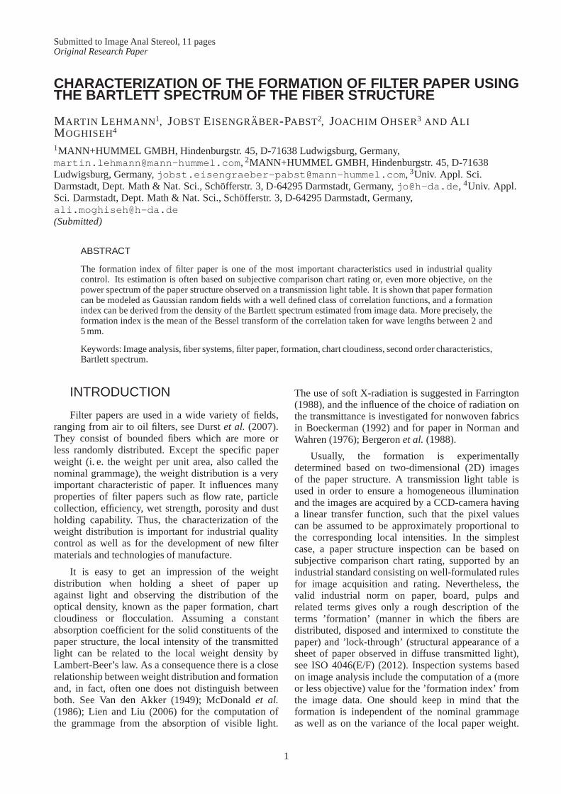
Fig. 4. A realization of the isotropic Boolean modelwith segments of exponentially distributed lengths,1/λ = 2mm, NA = 10mm−2; the width of the imageis 20 mm.

In the following we assume that the length ofthe segments is exponentially distributed with theparameterλ , see Fig. 4 for a realization. Then theBoolean modelΞ is uniquely characterized by theparameterλ of the exponential distribution and the

4


specific line lengthLA, i. e. the expectation of the totallength of the segments per unit area. Notice that 1/λis the mean fiber length, andNA = λLA is the meannumber of fibers per unit area. Then

g(r) = 1+λ

NAπre−λ r , r > 0

is the so-called pair correlation function ofΞ, definedas the density of the reduced second moment measurewhich is associated with random length measureL ofΞ, see p. 186 in Stoyanet al. (1995) for a formulaof the reduced second moment measureK of Booleansegment processes.

Let κ : R2 7→ R be a non-negative and boundedkernel function with

∫

R2 κ(x)dx = 1. By κ∗(x) =κ(−x) we denote the reflection ofκ , andκ ∗ f is theconvolution of the two functionsκ and f . Furthermore,let g : R 7→ R

2 be an arclength parametrization of afinite immersed curveϕ in R

2, that isϕ = g(s) : 0≤s≤ ℓ, whereg is twice continuous differentiable andℓ is the curve length. Then the convolutionϕ ∗κ maybe defined as

(

ϕ ∗κ)

(x) =

ℓ∫

0

κ(

x−g(s))

ds, x∈ R2.

Then Ψx =(

Ξ ∗ κ)

(x) is a macroscopicallyhomogeneous random field withEΨx = LA, but Ψxis not a GRF.

If we chooseκ such that it decreases sufficientlyfast as‖x‖ → ∞, then from the central limit theorem(CLT) it follows that

Φx = limNA→∞

1NA

(

Ξ∗κ −LA)

(x), x∈ R2

forms a GRF withµ = 0 and the covariance functioncov(x) = λ 2

(

(κ ∗κ∗)∗h)

(x) whereh(x) = g(‖x‖)−1.

Let now κεε>0 be a family of non-negativekernel functions of bounded support,κε(x) = 0 for‖x‖ ≤ 1

ε , then it follows that cov(x)→ σ2h(x) asε ↓ 0for all x∈ R

2.

In the line with the above, we are settingh1(r) =g(r)− 1 and callh1 the correlation function of theBoolean modelΞ. It holds thath1(r) → ∞ as r ↓ 0,and the corresponding covariance measure is positivedefinite, see Section 6.4 in Ohser and Schladitz (2009).This means that there exists a Bartlett spectrum ofΞ.Moreover, the Bartlett spectrum has a density, i. e. theBessel transform

h1(ρ) =1

πNA

λ√

λ 2+ρ2, ρ ≥ 0

of h1 exists, which is, up to a constant factor, the sameask1 given in (6) forν =−1

2. This is surpricing, sincethe curve shape ofh1 basically differs from that ofk1given in (5).

In other words, the GRFΦx inherits the secondorder properties of the Boolean modelΞ. Thisshows that there is a close relationship between’independent and uniform scattering’ of fibers inthe plane (observable on a microscale) and paperformation (observable on a mesoscale) where the fibermean length 1/λ corresponds to the formation index.Nevertheless, ’independent and uniform scattering’of fibers means that there is no tendency to formfiber clusters (flocks) induced e. g. by adhesion and,moreover, a significant formation is observable even ifthe fibers are ’independently and uniformly scattered’,see Fig. 5 for an example.

Fig. 5. A realization of a GRF based on an isotropicBoolean model with segments of exponentiallydistributed lengths,1/λ = 2mm, NA = 10mm−2,where the smoothing kernelκ is the probability densityof the isotropic 2D Gauss distribution withσ =0.02mm. The width of the image is 102.4 mm.

MONTE CARLO SIMULATION

We follow the spectral approach developedby Shinozuka and Jan (1972) and others, whererealizations of a GRF are generated based on thefollowing two steps:

1. Let u be a random number uniformly distributedon the interval[0,1], and letv be a random vectordistributed with respect to the probability measureΓΦ/2π on R

2. If u andv are independent randomvariables, then

Ψx =√

2cos(2πu+vx), x∈ R2

5


forms a macroscopically homogeneous andisotropic random field with the expectationµ = 0,the varianceσ2 = 1 and the correlation functionk.Notice thatΨx is not ergodic.

2. Let now Ψ(1)x , . . . ,Ψ(m)

x , m ∈ N, are pairwiseindependent and identically distributed randomfields withµ = 0, σ2 = 1 andk. Define

φ (m)x =

1√m

m

∑i=1

Ψ(i)x , x∈ R

2

then from the CLT it follows that

Φx = σ limm→∞

φ (m)x +µ , x∈ R

2

is a macroscopically homogeneous and isotropicGRF withµ , σ2 andk.

See Lantuejoul (2002) for further details and anoverview of alternative approaches.

But how large mustmbe such thatφ (m)x can be seen

as a realization ofΦx? The usual way for a suitablechoice ofm is based on the Berry-Esseen inequality

supx|φ (m)

x −Φx| ≤c

σ3√

m

with c < 0.4784, see Korolev and Shevtsova (2010).For the realizations of the GRFs shown in Figures 1 to3 the numberm was empirically chosen asm= 4096,which surely is large enough ask(ρ) vanishes rapidlyat infinity, see also the remark in Lantuejoul (2002),p. 192.

ESTIMATION OF k

In this section we assume that the Bartlett spectrumΓΦ of the observed random fieldΦx has a density.We are starting from the normalized random fieldf (x) = (Φx− µ)/σ having the expectation 0 and thevariance 1. In applications the functionf is observedthrough a compact windowW ⊂ R

2 with the indicatorfunction1W defined as1W(x)= 1 if x∈W and1W(x)=0 otherwise. This means that the masked functionfW(x) = f (x) · 1W(x) is considered. One should keepin the mind that the image data can be seen as arealization of fW, whereW is the (rectangular) imageframe. Furthermore, we introduce a window functioncW of W defined as the auto-correlation of the function1W, cW = 1W ∗1∗W.

The cW is bounded and of bounded support, andthus its Fourier transform ˆcW exists. This yields ananalogue to the Wiener-Khintchine theorem, that is

F (cW · k) = 2πE| fW|2. The power spectrumE| fW|2of fW is integrable, and hence its inverse FouriertransformF can be applied which yields

cW ·k= 2π F(

E| fW|2)

.

Assume now that the origin belongs toW. ThencW ispositive for allx belonging to the interior ofW, and itfollows that

2π F(

| fW|2)

(x)

cW(x)(7)

is an unbiased estimator ofk(x) for all x in the interiorof W.

In the isotropic case the rotation mean of anestimation ofk can be performed (rotation aroundthe origin), which gives an estimation of the radialfunction k1. From this, one obtains an estimation ofthe densityk1 of the Bartlett-Spectrum using the 1-dimensional Fourier-Bessel transform (3).

An overview of the estimation procedure is givenin Fig. 6. Clearly, kcW can also be computed bycorrelation (red marked path in Fig. 6).

?

?

-

-

?

F

Fourier transform

F

inverse Fouriertransform

Fourier-Besseltransform

f ·1W

1W

k ·cW

cW

k1

2π f ∗ 1W

1W

2πE| fW|2|1W|2

k1

∗∗

/cWrotation mean

E, | · |2

Fig. 6. Scheme of the computation of the densityfunction k1(ρ). The symbol∗∗ stands for auto-correlation of functions (convolution with the reflectedfunction).

It is well known that forn pixels of an image ofΦx, the correlation functionk can be computed usingthe Fast Fourier Transform (FFT) with a complexityin O(nlogn), where also the window function canefficiently be computed via the inverse space usingcW = F |F1W|2. In the rectangular case, the windowfunction is explicitly known from the literature, seee. g. Ohser and Mucklich (2000), p. 356. A discreteversion of the Bessel transform can be based onnumerical integration, e. g. by Romberg’s rule.

6


Unfortunately, the assumption of periodicity in thediscrete Fourier transform (dFT) causes an overlappingeffect (edge effect). This effect can be eliminated byexpanding the functionfW to the window 2W, wherefW is padded with zeros, that isf2W(x) = fW(x) ifx ∈ W, and f2W(x) = 0 if x ∈ 2W \W. This increasesthe pixel number to 4n, still the complexity of theFFT applied tof2W belongs toO(nlogn) which is aconsiderable gain compared to the usual estimation ofkcW based on auto-correlation, see Fig. 6 (red path).Notice that data windowing using a 2D analogue ofthe Welch, Hann (Hamming) or Bartlett window, seePresset al. (2007), avoids any window expansion, butthe unbiasedness of (7) gets lost.

The dFT (and its inverse) is usually based on amodified setting of the continuous Fourier transform.The main difference to be aware of, is that in (1) and(2) the frequencyξ is substituted with the angularfrequencyω = 2πξ . This has an impact on the scalingof the estimated spectral density.

Finally, we remark that the sampling off on ahomogeneous point lattice induces a sampling off onthe inverse lattice, where the relationship between theoriginal lattice and its inverse is as follows: LetU bea matrix for which the column vectors are forming abasis of the original lattice, then the column vectors ofthe matrix(U ′)−1 form a basis of the inverse lattice,Ohser and Schladitz (2009), p. 66. In terms of a dFTapplied to a 2D image withn1 ·n2 pixels of sizea1 ·a2,the transformed image also consists ofn1 · n2 pixelsbut of the size ˆa1 · a2, wherea1 = 1/(n1a1) anda2 =1/(n2a2).

-10 2 1 1/ρ [mm]

6

0

1

2

3k1 empirical

model,ν = 0.5model,ν = 1.0

-10 2 1 1/ρ [mm]

6

0

1

2

3k1 empirical


Fig. 7. Images showing the formations of the filterpapers Nr 1a (top) and Nr 1b (bottom), respectively,as well as the densities of their Bartlett spectra.

EXPERIMENTAL RESULTS

The applicability of the method presented aboveis now demonstrated for three filter papers producedby wet laid cellulose fibers. The material No. 1 has anominal grammage of 200 g/m2 and a mean thicknessof about 0.9 mm, the material No. 2 is of 90 g/m2

and about 0.25 mm thick, and the material No. 3 isof 170 g/m2 and about 0.7 mm thick. The mean fiberlength in these materials was much longer than 2 mm.

In order to estimate the spectral density and todetermine a formation index, various filter papersare scanned in the light transmission mode using aconventional CCD camera, see Figs. 7 to 9 (left) forexamples. The 8-bit gray-tone images are of 1580×1200 pixels with a lateral resolution of 0.177 mmper pixel and, thus, the effective image size amounts279.66×212.40mm2. The wet laying proces inducesa slight sheet inhomogeneity appearing as a long waveshading in the corresponding images. This shadingwas corrected based on a reference image which wasobtained by smoothing the image data using a largeGaussian filter with the parameterσ = 17.4 mm, andwhere the reference image was subtracted from theoriginal one.

-10 2 1 1/ρ [mm]

6

0

1

2

3k1 empirical


-10 2 1 1/ρ [mm]

6

0

1

2

3k1 empirical


Fig. 8. The filter papers Nr 2a (top) and Nr 2b(bottom).

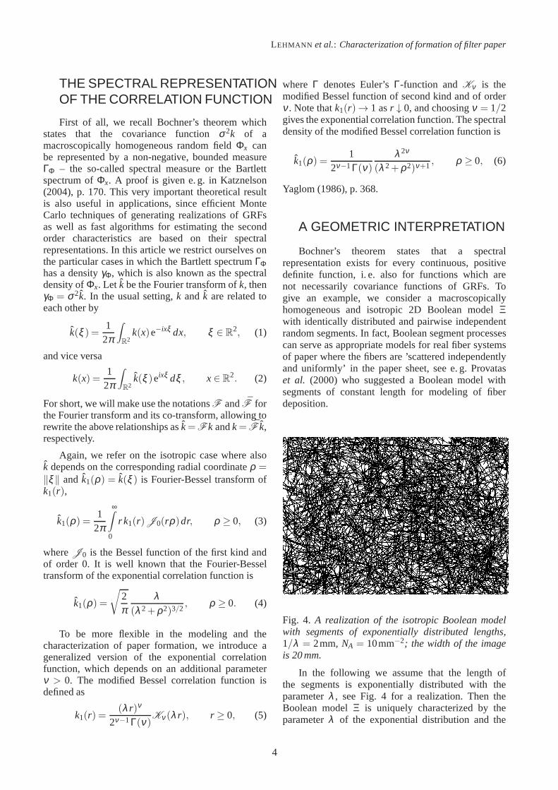
The functionk1 is estimated from the image datausing the method described in the previous section.The graphs of the estimates are shown in Figs. 7to 9 (right), wherek1 is given in mm2. We remarkthat the relative small values ofk1 for wave lengths1/ρ less than 10 mm might be consequence of theshading correction. Generally, it is a hard problemto remove an unknown long wave shading undersimultaneous keeping the spectrum of long waves in

7


the real structure. Furthermore, because of the datawindowing, even the fractions of long waves areestimated with a larger error than those of short waves.Nonetheless, from studies based on realizations ofGRFs with comparable spectral densities, it followsthat for wave lengths less than 10 mm, the functionk1is estimated from the image data with sufficiently smallerrors.

-10 2 1 1/ρ [mm]

6

0

1

2

3k1 empirical


-10 2 1 1/ρ [mm]

6

0

1

2

3k1 empirical


Fig. 9. The filter papers Nr 3a (top) and Nr 3b(bottom).

Obviously, there is a white noise observable as anadditive constantc of k1,

c= limρ→∞

k(ρ)≈ 0.33mm2

(the blue lines in Figs. 7 to 9, right). The reason forthis is not clear. Probably, a considerable fraction ofthis noise comes from image acquisition.

material specimen β λ [mm−1]nr. nr. [mm2] ν = 0.5 ν = 11 1a 2.6 0.550 0.5571 1b 2.3 0.564 0.5682 2a 1.9 0.689 0.6942 2b 2.1 0.632 0.6373 3a 2.2 0.615 0.6193 3b 2.1 0.635 0.638

Table 1. The formation indexβ and the numericalvaluesλ for the adapted function (6).

Moreover, for fixedν the theoretical function (6)was adapted to the experimental data forρ ≤ 10 mm,where the parameterλ was estimated based on a leastsquares method, see Figs. 7 to 9. The estimates ofλ are

widely independent ofν , see Tab. 1, and in the mostcases the fitting forµ = 1 is better than forµ = 1

2.

Finally, a formation indexβ is the determined asthe mean of the densityk1 for wave lengths between 2and 5 mm, which are relevant for industrial application.

DISCUSSION AND CONCLUSIONS

Throughout this article it is assumed that the paperstructure is isotropic, but most papers produced onpapermaking machines such as those based on theprinciples of the Fourdrinier Machine show a clearanisotropic formation, see also Schaffnit and Dodson(1993); Scharcanski and Dodson (1996; 2000) wherethe anisotropy of formation is discussed in detail.Here we only remark that anisotropic paper formationcorresponds to an anisotropic spectral densityk(ξ ),and from an estimate ofk one can derive two quantitiesβ1 andβ2 describing the paper formation. Let(ρ ,ϕ)denote the polar coordinates ofξ with ρ ≥ 0 and 0≤ϕ < π. Then the formation indexβ1 can be computedfrom k(ρ ,ϕ1), whereϕ1 is the processing direction ofpaper making, andβ2 is obtained fromk(ρ ,ϕ2) for thedirectionϕ2 perpendicular toϕ1. Usually,β1 is at leastβ2, andβ1 = β2 in the isotropic case.

For fixed ϕ1 and ϕ2, the functions k⊥1 (ρ) =

k(ρ ,ϕ1) and k⊥2 (ρ) = k(ρ ,ϕ2) can be seen as planarsections profiles of the spectral densityk(x). Fromthe projection slice theorem, see e. g. Kuba andHermann (2008), it immediately follows thatk⊥1 (ρ)and k⊥2 (ρ) can be obtained as a cosine transformof the orthogonal projectionsk⊥1 (r) resp. k⊥2 (r) ofthe estimated correlation functionk(x) onto thecorresponding section planes, i. e. the rotation mean inthe scheme of Fig. 6 is replaced with the orthogonalprojections onto the two section planes, and theFourier-Bessel transform is now a simple cosinetransform.

As pointed out in this article, there is a’basic formation’ related to an ’independent anduniform scattering’ of the paper fibers, and even this’basic formation’ can probably not be effected bytechnological measures. This means that the possibilityto reduce paper formation by an improved papermaking technology is strongly limited. Let us considera paper with a given formation, the question is asfollows: What is the difference between the givenand the ’basic’ formation? Unfortunately, the ’basicformation’ can be estimated only roughly from thedistribution of the fiber lengths and, until now thereis no save method to find out whether the formation ofa paper can be reduced or not.

8


The computation of the formation index fromimages of transmitted light via frequency space isvery efficient. However, the results from differentlaboratories are comparable only under the conditionthat the spectral density of the intensity of thetransmitted light is (nearly) the same as the spectraldensity of the local paper grammage. Thus, whenimplementing a laboratory system for industrialquality control one should take care of the wavelengthof the applied light, the homogeneity of illumination,the image acquisition, a possible inhomogeneity of thepaper, and the edge effects involved in the computationof the spectral density. It is very helpful to make testsas the following one: the increase of the paper weightshould not influence the formation and, therefore, thepaper formation of a single paper sheet must be thesame as that of a double sheet (both sheets of thesame formation and one sheets on top of the other).Furthermore, the estimation of the spectral densityshould be robust with respect to variations of the lateralresolution, i. e. varying the pixel size (in the range from0.05 to 0.2 mm) should lead to only small changes inthe estimated spectral density. Finally, the size of thepaper sheet (i. e. the size of the windowW) shouldbe large enough such that the statistical errors of theestimates are limited. From our experience we cansay that an A4-sheet is sufficient. More precisely, letΦx be a Gaussian random field with an exponentialcorrelation function,λ & 0.5mm−1, observed througha rectangular windowW of the size 210× 297mm2,then from simulation studies it follows that the relativestatistical error of an estimate ofk1(ρ) is less than 5 %for all wave lengths 1/ρ ≤ 5mm.

Acknowledgement

This work was supported by the German FederalMinistry of Education and Research (BMBF) undergrant MNT/03MS603C/AMiNa.

REFERENCES

Abrahamsen P (1985). A review of random fieldsan correlation functions, 2nd ed. Tech. Rep. 314,Blindern, Oslo.

Adler RJ (1981). The Geometry of Random Fields.New York: John Wiley & Sons.

Adler RJ, Taylor J (2007). Random Fields andGeometry. New York: Springer.

Alava M, Niskanen K (2006). The physics of paper.Rep Prog Phys 69:669–723.

Antoine C (2000). GRACE, a new tool to simulatepaper optical properties. In: van Lieshout M, ed.,New Characterisation Models for Fibres, Pulp andPaper Sci. Joint Publication of the COST ActionE11 Working Group Paper.

Bergeron M, Bouley R, Drouin B, Gagnon R(1988). Simultaneous moisture and basis weightmeasurement. Pulp and Paper Magazine of Canada89:173–6.

Boeckerman PA (1992). Meeting the specialrequirements for on-line basis weightmeasurements of lightweight nonwoven fabrics.Tappi J :166–72.

Burt BJ, Adelson EH (1983). The Laplacian pyramidas a compact image code. IEEE Trans Comm31:532–40.

Cherkassky A (1998). Analysis and simulationof nonwoven irregularity and nonhomogeneity.Textile Res J 68:242–53.

Cherkassky A (1999). Evaluating nonwoven fabricirregularity on the basis of Linnik functionals.Textile Res J 69:701–8.

Chinga-Carrasco G (2009). Exploring the multi-scalestructure of printing paper – a review of moderntechnology. J Microsc 234:211–42.

Cresson TM (1988). The Sensing, Analysis andSimulation of Paper Formation. Ph.D. thesis, StateUniversity, New York.

Cresson TM, Luner P (1990a). The characterizationof paper formation, Part 2: The texture analysis ofpaper formation. Tappi J 12:175–84.

Cresson TM, Luner P (1990b). Description of thespatial gray level dependence method algorithm.Tappi J 12:220–2.

Drouin B, Gagnon R, Cheam C, Silvy J (2001). A newway for testing paper sheet formation. Compos SciTechn 61:389–91.

Durst M, Klein GM, Moser N, Trautmann P (2007).Filtration und Separation in der Automobiltechnik.Chem Ing Techn 79:1845–60.

Farrington TE (1988). Soft X-ray imaging can beused to asses sheet formation and quality. TappiJ 71:140–4.

Gregersen ØW, Niskanen K (2000). Measurement andsimulation of paper 3D-structure. In: van LieshoutM, ed., New Characterisation Models for Fibres,Pulp and Paper. Joint Publication of the COSTAction E11 Working Group Paper.

ISO 4046(E/F) (2012). International standardon paper, board, pulps and related terms –Vocabularity, Part 1–5. ISO Copyright Office,Geneva.

Kallmes OJ (1984). The measurement of formation.Tappi J 67:117–.

Katznelson Y (2004). An Introduction to HarmonicAnalysis. Cambridge Mathematical Library.Cambridge: Cambridge University Press, 3rd ed.

9


Koch K, Ohser J, Schladitz K (2003). Spectraltheory for random closed sets and estimating thecovariance via frequency space. Adv Appl Prob35:603–13.

Korolev VY, Shevtsova IG (2010). On the upperbound for the absolute constant in the Berry-Esseen inequality. Theory of Prob and its Appl54:638–658.

Kuba A, Hermann G (2008). Some mathematicalconcepts for tomographic reconstruction. In:Banhart J, ed., Advanved Tomographic Methodsin Materials Science and Engineering. Oxford:Oxford University Press, 19–36.

Lantuejoul C (2002). Geostatistical Simulation –Models and Algorithms. Berlin: Springer.

Lien HC, Liu CH (2006). A method of inspecting non-woven basis weight using the exponential law ofabsorption and image processing. Textile Res J76:547–58.

McDonald JD, Rarrell WR, Stevens RK, HussainSM, Roche AA (1986). Using an on-line lighttransmission gauge to identify the source ofgrammage variations. J Pulp and Paper Sci 12:J1–J9.

Norman B (1986). The formation of paper sheets,Chapter 6. In: A. BJ, Kolseth P, eds., Paper,Structure and Properties, vol. 8 ofInt. Fiber Sci.and Techn. Series. Marcel Dekker Inc.

Norman B, Wahren D (1976). Mass distributionand sheet properties of paper. In: FundamentalProperties of Paper to its End Uses, Trans. Symp.London: B.P.B.I. F.

Ohser J, Mucklich F (2000). Statistical Analysis ofMicrostructures in Materials Science. Chichester,New York: J Wiley & Sons.

Ohser J, Schladitz K (2009). 3D Images of MaterialsStructures – Processing and Analysis. Weinheim,Berlin: Wiley VCH.

Pourdeyhimi B, Kohel L (2002). Area-based strategyfor determining web uniformity. Textile Res J72:1065–72.

Praast H, Gottsching L (1991). Formation graphischerPapiere. Das Papier 45:333–47.

Press WH, Teukolsky SA, Vetterling WT, Flannery BP(2007). Numerical Recipes – The Art of ScientificComputating, 3rd Ed. Cambridge University Press.

Provatas N, Alava MJ, Ala-Nissila T (1996). Densitycorrelations in paper. Phys Rev E 54:R36–R38.

Provatas N, Haataja M, Asikainen J, Majaniemi S,Alava M, Ala-Nissila T (2000). Fiber depositionmodels in two and three dimensions. Colloids andSurfaces A 165:209–29.

Robertson AA (1956). The measurement of paperformation. Pulp and Paper Magazine of Canada55:119–27.

Sampson WW (2009). Modelling StochasticFibrous Materials with Mathematica. EngineeringMaterials and Processes. London: Springer.

Sara H (1978). The Characterization and Measurementof Paper Formation with Standard Deviation andPower Spectrum. Ph.D. thesis, Helsinki University,Helsinki.

Schaffnit C, Dodson CTJ (1993). A new analysisof fiber orientation effects on paper formation.Paperija Puu 75:68–75.

Scharcanski J (2006). Stochastic texture analysisfor measuring sheet formation variability in theindustry. IEEE Trans Instrum Measurement55:1778–85.

Scharcanski J, Dodson CTJ (1996). Texture analysisfor estimating spatial variability and anisotropy inplanar structures. Opt Eng J 35:2302–8.

Scharcanski J, Dodson CTJ (2000). Stochastic textureimage estimators for local spatial anisitropy andits variability. IEEE Trans Instrum Measurement49:971–9.

Scholz M, Claus B (1999). Analysis and simulation ofnonwoven textures. Z Angew Math Mech 79:237–40.

Shinozuka M, Jan CM (1972). Digital simulation ofrandom processes and its applications. J SoundVibration 25:111–28.

Stoyan D, Kendall W, Mecke J (1995). StochasticGeometry and Its Applications. Chichester:J. Wiley & Sons, 2nd ed.

Van den Akker JA (1949). Scattering and absorptionof light in paper and other diffusing media. Tappi32:498–501.

Wang X, Georganas ND, Petriu EM (2011). Fabrictexture analysis using computer vision techniques.IEEE Trans Instr Measurement 60:44–56.

Waterhouse JF, Hall MS, Ellis RL (1991). Strengthimprovement and failure mechanisms, 2.Formation. Tech. Rep. Project 3469, ReportII, Institute of Paper Science and Technology(API), Atlanta, Gorgia.

Xu B (1996). Identifying fabric structures withfast Fourier transform techniques. Textile Res J66:496–506.

Yaglom AM (1986). Correlation Theory of Stationaryand Related Random Functions I: Basic Results.Springer Series in Statistics. New York: Springer.

Yuhara T, Hasuike M, Murakami K (1986).Application of image processing technique

10


for analysis on sheet structure of paper, Part 1:quantitative evaluation of 2-dimensional mass

distribution. Japan Tappi 40:85–91.

11

characterization of the formation of filter paper...

Documents