characterization of neutron and proton exposure on the
TRANSCRIPT

Air Force Institute of TechnologyAFIT Scholar
Theses and Dissertations Student Graduate Works
3-23-2017
Characterization of neutron and proton exposureon the radiation resistant bacterium, deinococcusradioduransRonald C. Lenker
Follow this and additional works at: https://scholar.afit.edu/etd
Part of the Biological and Chemical Physics Commons, and the Nuclear Commons
This Thesis is brought to you for free and open access by the Student Graduate Works at AFIT Scholar. It has been accepted for inclusion in Theses andDissertations by an authorized administrator of AFIT Scholar. For more information, please contact [email protected].
Recommended CitationLenker, Ronald C., "Characterization of neutron and proton exposure on the radiation resistant bacterium, deinococcus radiodurans"(2017). Theses and Dissertations. 1623.https://scholar.afit.edu/etd/1623
CHARACTERIZATION OF NEUTRON AND PROTON EXPOSURE ON THE RADIATION RESISTANT BACTERIUM, DEINOCOCCUS RADIODURANS
THESIS
Ronald C. Lenker, Major, USA
AFIT-ENP-MS-17-M-100
DEPARTMENT OF THE AIR FORCE AIR UNIVERSITY
AIR FORCE INSTITUTE OF TECHNOLOGY
Wright-Patterson Air Force Base, Ohio
DISTRIBUTION STATEMENT A. APPROVED FOR PUBLIC RELEASE; DISTRIBUTION UNLIMITED.

The views expressed in this thesis are those of the author and do not reflect the official policy or position of the United States Air Force, Department of Defense, or the United States Government. This material is declared a work of the U.S. Government and is not subject to copyright protection in the United States.
AFIT-ENP-MS-17-M-100
CHARACTERIZATION OF NEUTRON AND PROTON EXPOSURE ON THE RADIATION RESISTANT BACTERIUM, DEINOCOCCUS RADIODURANS
THESIS
Presented to the Faculty
Department of Engineering Physics
Graduate School of Engineering and Management
Air Force Institute of Technology
Air University
Air Education and Training Command
In Partial Fulfillment of the Requirements for the
Degree of Master of Science in Nuclear Engineering
Ronald C. Lenker, MS
Major, USA
March 2017
DISTRIBUTION STATEMENT A. APPROVED FOR PUBLIC RELEASE; DISTRIBUTION UNLIMITED.
AFIT-ENP-MS-17-M-100
CHARACTERIZATION OF NEUTRON AND PROTON EXPOSURE ON THE RADIATION RESISTANT BACTERIUM, DEINOCOCCUS RADIODURANS
Ronald C. Lenker, MS
Major, USA
Committee Membership:
Douglas R. Lewis, LTC, USA, PhD Chair
Justin A. Clinton, PhD Member
Roland J. Saldanha, PhD Member
iv
AFIT-ENP-MS-17-M-100
Abstract
Deinococcus radiodurans is a robust bacterium that is known for its extraordinary
resistance to ionizing radiation. In general, many of the investigations of this bacterium’s
resistance have revolved around low linear energy transfer radiation, such as gamma and
electron radiation. This study explored Deinococcus radiodurans’s ability to survive
high linear energy transfer radiation, specifically proton and neutron radiation.
Deinococcus radiodurans was dehydrated to reduce the effects of low linear energy
transfer radiation. The bacteria were exposed to both neutron and proton radiation of
varying amounts and rehydrated. The resulting colonies were counted and compared to
colonies of non-irradiated control samples using a two population, t-statistic test. With
few, non-trend forming exceptions, the results of these comparisons showed, with 95%
certainty, that there was no statistical difference between the non-irradiated controls and
the irradiated samples.
v
Acknowledgments
I would like to express my sincere appreciation to my faculty advisor, the faculty of ENP,
and the scientists and researchers of USAFSAM and the Sandia Ion Beam Laboratory.
Ronald C. Lenker
vi
Table of Contents
Page
Abstract .............................................................................................................................. iv
Table of Contents ............................................................................................................... vi
List of Figures .................................................................................................................. viii
List of Tables .......................................................................................................................x
I. Introduction .....................................................................................................................1
General Issue ................................................................................................................1
Problem Statement ........................................................................................................2
Hypothesis ....................................................................................................................2
Research Objectives .....................................................................................................2
Assumptions/Limitations ..............................................................................................3
II. Literature Review ............................................................................................................4
Chapter Overview .........................................................................................................4
A Brief Description of Deinococcus radiodurans ........................................................4
High LET and Low LET ..............................................................................................6
Direct and Indirect Action ............................................................................................7
DNA .............................................................................................................................8
DNA Damage from Direct and Indirect Actions ..........................................................9
Deinococcus radiodurans DNA Damage and Repair ................................................10
Deinococcus radiodurans and Mutant Strains ...........................................................11
III. Methodology ................................................................................................................13
Chapter Overview .......................................................................................................13
Deinococcus Radiodurans Sample Preparation .........................................................13
Neutron Dose Calculations .........................................................................................21
vii
Neutron Irradiation of Samples ..................................................................................23
Rehydration of Samples and Spotting Post Neutron Irradiation ................................26
Colony Counting Post Neutron Irradiation .................................................................27
Proton Generation .......................................................................................................28
Proton Dose Calculations ...........................................................................................28
Rehydration of Samples and Spotting Post Proton Irradiation ...................................35
Colony Counting Post Proton Irradiation ...................................................................35
Statistical Methods of Comparison ............................................................................36
IV. Analysis and Results ....................................................................................................37
Chapter Overview .......................................................................................................37
1st and 2nd Neutron Experiments .................................................................................38
3rd Neutron Experiment ..............................................................................................42
1st, 2nd, 3rd Neutron Experiments Findings .................................................................45
Proton Experiment ......................................................................................................46
V. Conclusions and Recommendations ............................................................................48
Conclusions of Research ............................................................................................48
Recommendations for Future Research ......................................................................51
Appendix A: Optical Density Measurements ...................................................................53
Appendix B: Neutron Dose Calculations ..........................................................................57
Appendix C: Proton Dose Calculations ............................................................................58
Appendix D: QASAR-3 Parameters .................................................................................59
Appendix E: Deinococcus Radiodurans Statistical Analysis ...........................................65
Bibliography ......................................................................................................................85
viii
List of Figures
Page
Figure 1. Deinococcus radiodurans taken by SEM at USAFSAM. .................................. 5
Figure 2. Two stages of genome reconstitution in Deinococcus radiodurans.[11] ......... 11
Figure 3. This array depicts the location of each strain of Dr. Each strain (represented by
number, i.e. 1 is WT, 5 is Mutant #5, etc.) was separated from the others by a row.
This setup allowed for twelve samples per strain. ..................................................... 16
Figure 4. 60µl drop of Deinococcus radiodurans at 2-5 x 10⁸ CFUs / ml count taken by
SEM at USAFSAM. ................................................................................................... 17
Figure 5. For this experiment, fewer samples were used, but EC was included. Four
samples per strain of bacteria were placed on each plate. .......................................... 18
Figure 6. The samples in columns 1-8, rows A, C, E, and G were set to receive various
amounts of irradiation. These rows set to receive 100, 500, 1000, 2500 Gy
respectively. All samples in column 12 did not receive any radiation. The 1 in each
box represents wild type, but plates with the other mutants were also constructed. .. 19
Figure 7. Rows A, C, E, and G held WT, mutant 5, 8, and 11 respectively. ................... 20
Figure 8. Two samples plates on the neutron generator. .................................................. 24
Figure 9. 4 treatment plates for irradiation by the neutron generator. ............................. 25
Figure 10. Wild Type Deinococcus radiodurans following a five hour neutron treatment
in the 1st Neutron experiment. .................................................................................... 27
Figure 11. Input screen for TRIM, with the first layer of Dr and the second layer the
plate lid. ...................................................................................................................... 29
ix
Figure 12. Based on the inputs in the previous figure, TRIM simulation of 4.5 MeV
proton ions irradiating the Dr sample. ........................................................................ 30
Figure 13. Dr sample plate attached to the stage of the QASPR-3. ................................. 33
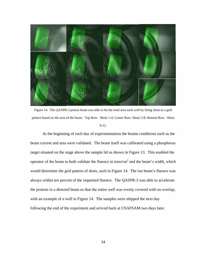
Figure 14. The QASPR-3 proton beam was able to hit the total area each well by firing
shots in a grid pattern based on the area of the beam. Top Row: Shots 1-4; Center
Row: Shots 5-8; Bottom Row: Shots 9-12. ............................................................... 34
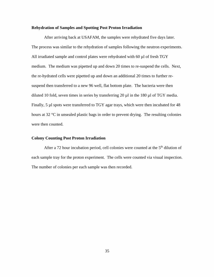
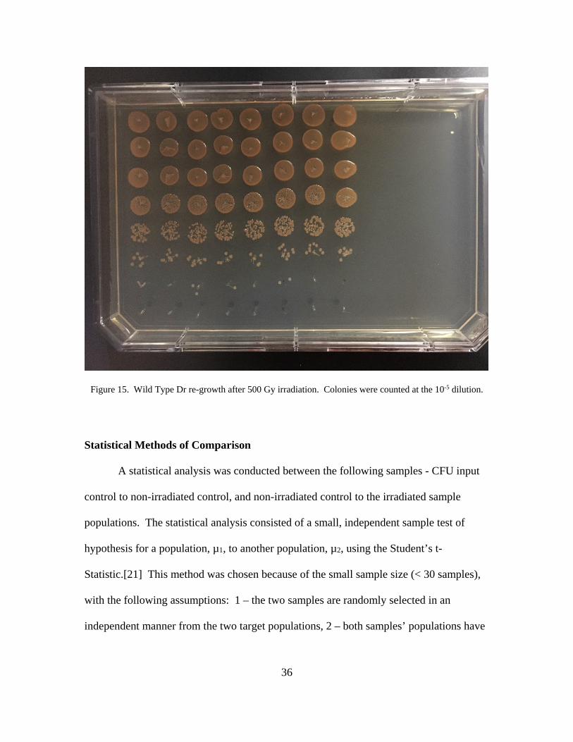
Figure 15. Wild Type Dr re-growth after 500 Gy irradiation. Colonies were counted at
the 10-5 dilution. ......................................................................................................... 36
Figure 16. Total CFU comparison for the 1st Neutron Experiment. ................................ 38
Figure 17. Dr Wild Type untreated with neutron radiation – 1st Neutron Experiment .... 40
Figure 18. Dr Wild Type neutron irradiated for 5 hours – 1st Neutron Experiment ........ 40
Figure 19. Total CFU comparison for the 2nd Neutron Experiment. ............................... 41
Figure 20. Total CFU comparison for the 3rd Neutron Experiment. ................................ 42
Figure 21. EC CFU input control, with countable colonies at the 10-5 dilution .............. 44
Figure 22. EC untreated control, with countable colonies at the 10-2 dilution. ............... 44
Figure 23. EC at 5 hours of neutron treatment. ................................................................ 45
Figure 24. Total CFU comparison for the Proton Experiment. ....................................... 46
x
List of Tables
Page
Table 1. Deinococcus radiodurans R1 Stain List ............................................................ 12
Table 2. Deinococcus radiodurans Cell Composition ..................................................... 22
Table 3. Neutron Dose per Well ....................................................................................... 23
Table 4. Proton Dose per Well .......................................................................................... 32
Table 5. 1st Neutron Experiment Statistically Significant Population Comparisons ....... 39
Table 6. 2nd Neutron Experiment Statistically Significant Population Comparisons ...... 41
Table 7. 3rd Neutron Experiment Statistically Significant Population Comparisons ....... 43
Table 8. Proton Experiment Statistically Significant Population Comparisons .............. 47
Table 9. Estimated Number of Deinococcus radiodurans DSBs at an LET of 8.5 keV/µm
.................................................................................................................................... 49
Table 10. Estimated Number of Deinococcus radiodurans DSBs at an LET of 62.4
keV/µm ....................................................................................................................... 50
Table 11. Initial Dr Optical Densities and Required Culture for an OD600 of 0.25 for 1st
Neutron Experiment ................................................................................................... 53
Table 12. Initial Dr Optical Densities and Required Culture for an OD600 of 0.25 for 2nd
Neutron Experiment ................................................................................................... 53
Table 13. Initial Dr Optical Densities and Required Culture for an OD600 of 0.25 for 3rd
Neutron Experiment ................................................................................................... 54
Table 14. Initial Dr Optical Densities and Required Culture for an OD600 of 0.25 for
Proton Irradiation Experiment .................................................................................... 54
xi
Table 15. Post 4 Hour Incubation Optical Density and Amount of TGY required to
achieve an OD600 of 5 for 1st Neutron Experiment .................................................... 55
Table 16. Post 4 Hour Incubation Optical Density and Amount of TGY required to
achieve an OD600 of 5 for 2nd Neutron Experiment .................................................... 55
Table 17. Post 4 Hour Incubation Optical Density and Amount of TGY required to
achieve an OD600 of 5 for 3rd Neutron Experiment .................................................... 56
Table 18. Post 4 Hour Incubation Optical Density and Amount of TGY required to
achieve an OD600 of 5 for Proton Irradiation Experiment .......................................... 56
1
CHARACTERIZATION OF NEUTRON AND PROTON EXPOSURE ON
THE RADIATION RESISTANT BACTERIUM, DEINOCOCCUS RADIODURANS
I. Introduction
General Issue
Successfully surviving and navigating an irradiated battlefield, searching for
survivors at the location of a nuclear reactor meltdown, or continuing to explore our solar
system all involve exposure to ionizing radiation. As such, there continues to be a need
within the United States Department of Defense and other governmental organizations to
develop medical capabilities to either prevent or neutralize the biological damage caused
by ionizing radiation. The Defense Threat Reduction Agency has a multiyear BAA for
Basic Research for Combating Weapons of Mass Destruction (HDTRA-11-12-
BRCWMD-BAA) to include “advancing knowledge to protect life.”[1] The National
Institute of Health also has research goals aligned to this endeavor, with “Determining
mechanisms for radiation protection, mitigation and treatment.”[1]
By investigating the mechanisms behind Deinococcus radiodurans’s (Dr)
remarkable ability to resist ionizing radiation, we may further the understanding of how
to protect human cells from the dangers of ionizing radiation. Specifically, investigations
will be made into Dr’s survivability in a neutron and proton environment, experiencing
high linear energy transfer (LET) radiation.
2
Problem Statement
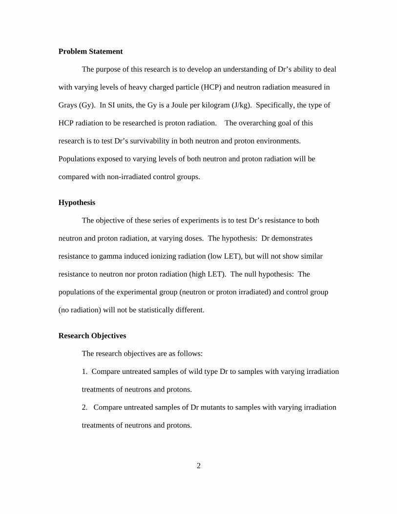
The purpose of this research is to develop an understanding of Dr’s ability to deal
with varying levels of heavy charged particle (HCP) and neutron radiation measured in
Grays (Gy). In SI units, the Gy is a Joule per kilogram (J/kg). Specifically, the type of
HCP radiation to be researched is proton radiation. The overarching goal of this
research is to test Dr’s survivability in both neutron and proton environments.
Populations exposed to varying levels of both neutron and proton radiation will be
compared with non-irradiated control groups.
Hypothesis
The objective of these series of experiments is to test Dr’s resistance to both
neutron and proton radiation, at varying doses. The hypothesis: Dr demonstrates
resistance to gamma induced ionizing radiation (low LET), but will not show similar
resistance to neutron nor proton radiation (high LET). The null hypothesis: The
populations of the experimental group (neutron or proton irradiated) and control group
(no radiation) will not be statistically different.
Research Objectives
The research objectives are as follows:
1. Compare untreated samples of wild type Dr to samples with varying irradiation
treatments of neutrons and protons.
2. Compare untreated samples of Dr mutants to samples with varying irradiation
treatments of neutrons and protons.
3
Assumptions/Limitations
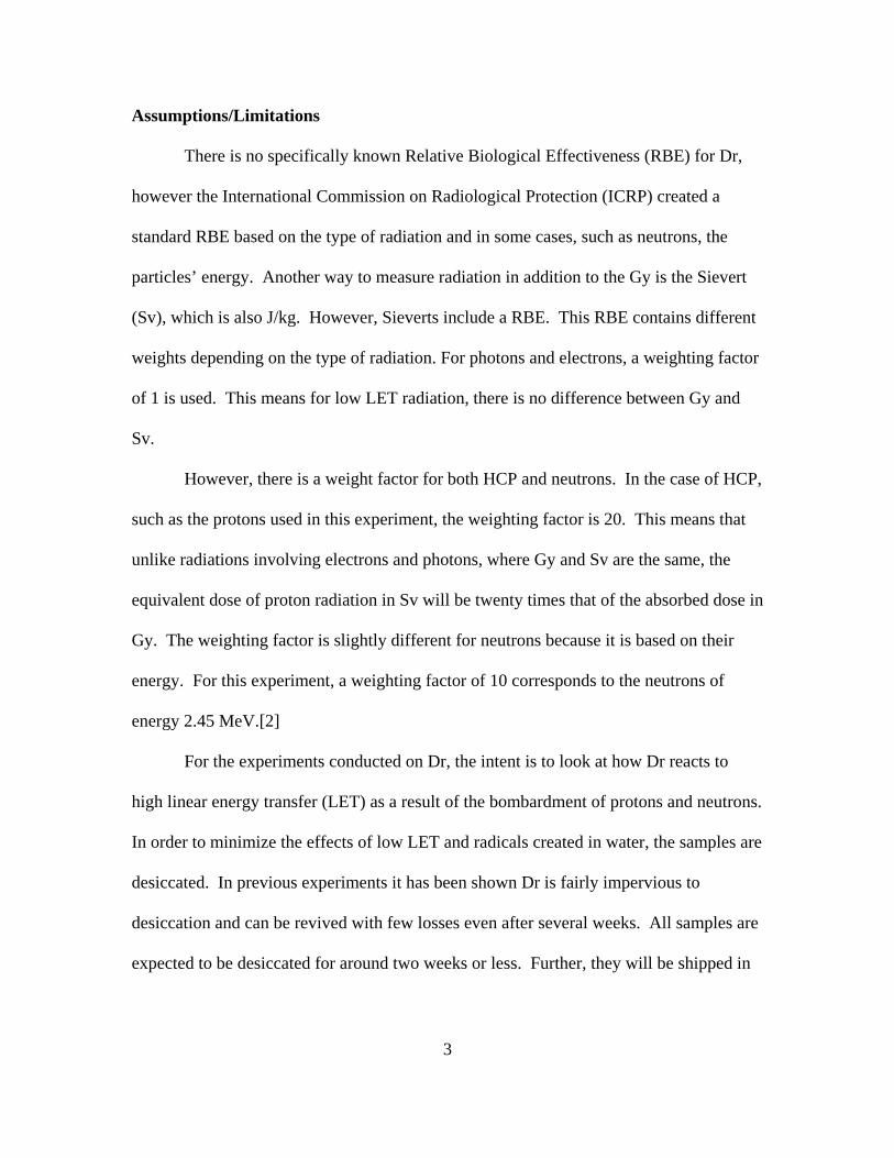
There is no specifically known Relative Biological Effectiveness (RBE) for Dr,
however the International Commission on Radiological Protection (ICRP) created a
standard RBE based on the type of radiation and in some cases, such as neutrons, the
particles’ energy. Another way to measure radiation in addition to the Gy is the Sievert
(Sv), which is also J/kg. However, Sieverts include a RBE. This RBE contains different
weights depending on the type of radiation. For photons and electrons, a weighting factor
of 1 is used. This means for low LET radiation, there is no difference between Gy and
Sv.
However, there is a weight factor for both HCP and neutrons. In the case of HCP,
such as the protons used in this experiment, the weighting factor is 20. This means that
unlike radiations involving electrons and photons, where Gy and Sv are the same, the
equivalent dose of proton radiation in Sv will be twenty times that of the absorbed dose in
Gy. The weighting factor is slightly different for neutrons because it is based on their
energy. For this experiment, a weighting factor of 10 corresponds to the neutrons of
energy 2.45 MeV.[2]
For the experiments conducted on Dr, the intent is to look at how Dr reacts to
high linear energy transfer (LET) as a result of the bombardment of protons and neutrons.
In order to minimize the effects of low LET and radicals created in water, the samples are
desiccated. In previous experiments it has been shown Dr is fairly impervious to
desiccation and can be revived with few losses even after several weeks. All samples are
expected to be desiccated for around two weeks or less. Further, they will be shipped in
4
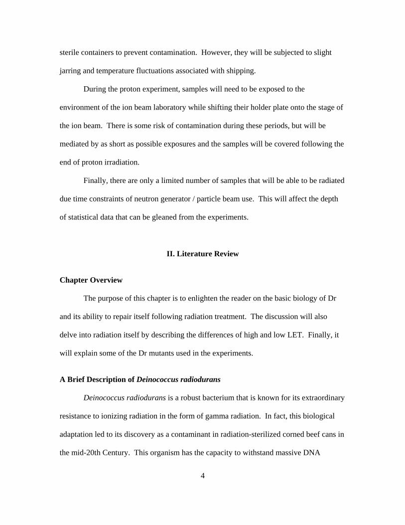
sterile containers to prevent contamination. However, they will be subjected to slight
jarring and temperature fluctuations associated with shipping.
During the proton experiment, samples will need to be exposed to the
environment of the ion beam laboratory while shifting their holder plate onto the stage of
the ion beam. There is some risk of contamination during these periods, but will be
mediated by as short as possible exposures and the samples will be covered following the
end of proton irradiation.
Finally, there are only a limited number of samples that will be able to be radiated
due time constraints of neutron generator / particle beam use. This will affect the depth
of statistical data that can be gleaned from the experiments.
II. Literature Review
Chapter Overview
The purpose of this chapter is to enlighten the reader on the basic biology of Dr
and its ability to repair itself following radiation treatment. The discussion will also
delve into radiation itself by describing the differences of high and low LET. Finally, it
will explain some of the Dr mutants used in the experiments.
A Brief Description of Deinococcus radiodurans
Deinococcus radiodurans is a robust bacterium that is known for its extraordinary
resistance to ionizing radiation in the form of gamma radiation. In fact, this biological
adaptation led to its discovery as a contaminant in radiation-sterilized corned beef cans in
the mid-20th Century. This organism has the capacity to withstand massive DNA
5
damage inflicted by ionizing radiation. For example, Bruch, et al. tested a Mn(II)
speciation of Dr with doses up to 10 kGy of gamma rays with only a two log kill
lethality.[3] “Well-aerated, exponential-phase cultures...will survive 5000 Gy of gamma
radiation without loss of viability, and survivors are routinely recovered from cultures
exposed to as much as 20 kGy”.[4] The mechanisms for this biological adaptation are
still being investigated, though they are suspected to be related to its DNA, its protective
proteins, or as a by-product of its ability to overcome severe desiccation.[5]
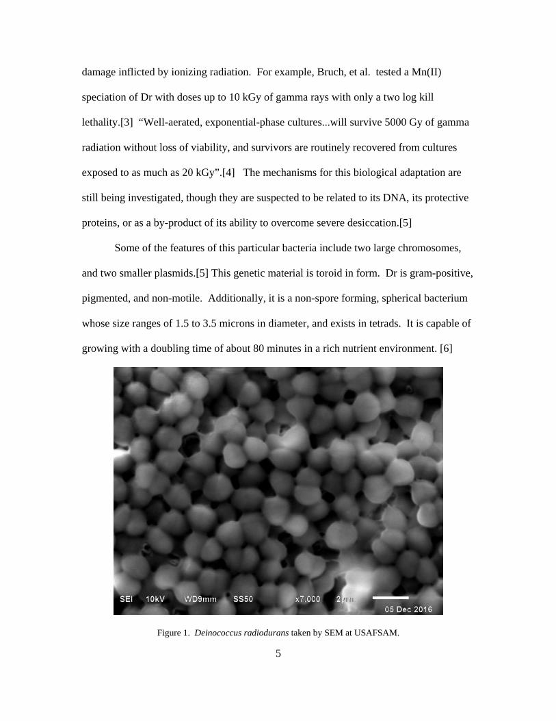
Some of the features of this particular bacteria include two large chromosomes,
and two smaller plasmids.[5] This genetic material is toroid in form. Dr is gram-positive,
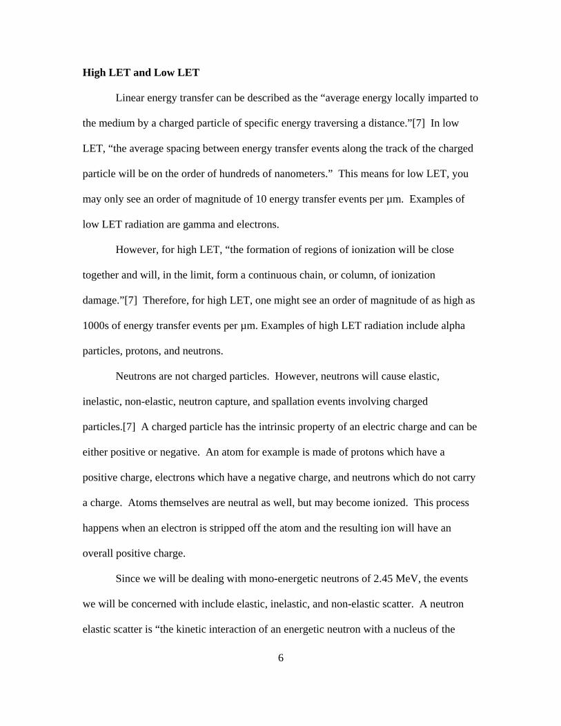
pigmented, and non-motile. Additionally, it is a non-spore forming, spherical bacterium
whose size ranges of 1.5 to 3.5 microns in diameter, and exists in tetrads. It is capable of
growing with a doubling time of about 80 minutes in a rich nutrient environment. [6]
Figure 1. Deinococcus radiodurans taken by SEM at USAFSAM.
6
High LET and Low LET
Linear energy transfer can be described as the “average energy locally imparted to
the medium by a charged particle of specific energy traversing a distance.”[7] In low
LET, “the average spacing between energy transfer events along the track of the charged
particle will be on the order of hundreds of nanometers.” This means for low LET, you
may only see an order of magnitude of 10 energy transfer events per µm. Examples of
low LET radiation are gamma and electrons.
However, for high LET, “the formation of regions of ionization will be close
together and will, in the limit, form a continuous chain, or column, of ionization
damage.”[7] Therefore, for high LET, one might see an order of magnitude of as high as
1000s of energy transfer events per µm. Examples of high LET radiation include alpha
particles, protons, and neutrons.
Neutrons are not charged particles. However, neutrons will cause elastic,
inelastic, non-elastic, neutron capture, and spallation events involving charged
particles.[7] A charged particle has the intrinsic property of an electric charge and can be
either positive or negative. An atom for example is made of protons which have a
positive charge, electrons which have a negative charge, and neutrons which do not carry
a charge. Atoms themselves are neutral as well, but may become ionized. This process
happens when an electron is stripped off the atom and the resulting ion will have an
overall positive charge.
Since we will be dealing with mono-energetic neutrons of 2.45 MeV, the events
we will be concerned with include elastic, inelastic, and non-elastic scatter. A neutron
elastic scatter is “the kinetic interaction of an energetic neutron with a nucleus of the
7
absorbing medium in which classical kinematics describes the energy transfer. The
elastic scattering process is important for neutrons with energies up to 14 MeV or so.”[7]
For neutrons that undergo inelastic scatter, the process is slightly different. In this case,
an initial neutron will be absorbed within a target nucleus, creating a short-lived
compound nucleus which then re-emits a neutron. This reaction will only occur if the
initial neutron’s energy “is greater than the threshold energy necessary for conservation
of energy and momentum.”[7] Finally, a non-elastic scatter is similar to an inelastic
scatter, but after the neutron is captured, the re-emitted particle is not another neutron.[7]
At this time, there has been very little experimentation involving high LET radiation and
Dr.
Direct and Indirect Action
Both high LET and low LET can result in either direct or indirect action. In the
case of indirect damage, the ionization and excitation of water by beta (electrons),
gamma (photons), and HCP radiation result in the creation of radical species. For
example, energetic photons may cause water to enter an excited state, then dissociate in
H∙ and OH∙ radicals. Likewise, ionization of water results in H20+ and e-. These products
will go on to interact with other water molecules and hydrogen to form other radicals
such as H20-, H∙, and eaq-.[7] These radicals then attack cellular components including
DNA.
In regards to direct damage, Alpen states, “Of greater importance with high LET
radiations is the high likelihood that an ionizing event will occur directly in the important
8
target bioactive molecule.”[7] In this study, the bioactive molecule of consideration is
deoxyribonucleic acid (DNA).
DNA
DNA is the genetic code found in all living organisms. The complex molecule’s
shape is that of a double-helix whose spiral is made up of two strands of monomer
nucleotides. These nucleotides consist of a deoxyribose sugar molecule that is covalently
bonded to a phosphate molecule, forming a sort of phosphate-sugar backbone. Like the
rungs on a twisted ladder, this backbone also has base pair steps. Each base pair is a
combination of a purine and a pyrimidine bound through hydrogen bonding. The purine
Adenine bonds with the pyrimidine Thymine. Likewise, the purine Guanine bonds with
the pyrimidine Cytosine. The order of the bases pairs forms the genetic code which tells
a cell how to form the proteins necessary for cellular functions.[8]
The bases and sugar molecules of the DNA present targets, which both can
undergo chemical reactions from the radicals mentioned in the previous section. The
more damaging attack however, is when these radicals break the covalent bond between
the sugar and phosphate molecules on the backbone. If this type of damage occurs to the
DNA, the result may be either a single strand break (SSB) or a double strand break
(DSB). In the case of a SSB, one of the two strands of DNA are severed. For DSBs,
both DNA strands are severed in proximity of each other, usually within 10 base pairs or
less. If a cell is unable to repair either a SSB or a DSB, the genetic code may be unusable
by the cell. Without this information, mutations may occur or the cell may be unable to
produce proteins needed for survival, resulting in cell death. Specifically, “for simpler
9
organisms, such as bacteriophages and viruses...measurement of DSBs in organisms with
double-stranded DNA precisely correlate with biological inactivation.”[7]
DNA Damage from Direct and Indirect Actions
DNA damage may result from either direct or indirect damage. In general, a
cell’s DNA exposed to high LET often receives numerous DSBs, which completely sever
the DNA. This is due to the more numerous events per distance as mentioned earlier.
DSBs are “far more serious in the consequences for a cell…and repair of DSBs is an
error-prone process that will frequently lead to mutation in the genome and/or loss of
reproductive capacity.”[7]
Indirect damage to DNA is the result of radicals created during indirect events.
Low LET is usually the cause of the “indirect action of the products of radiolysis” which
can result in SSBs.[7] SSBs are more readily repaired, though multiple SSBs in
proximity can result in DSBs. Alpen further states, “it has been suggested that the high
LET radiation…produces its damaging effect by production of double-strand breaks as
single events, whereas low LET radiation is thought to produce a preponderance of
damage through interaction of two sublethal events.”[7]
Numerous studies involving low LET radiation (such as gamma and electrons)
have led to further questions about Dr’s radio-resistance. Is Dr able to survive due to
having several copies of DNA available, the production of unique proteins which provide
more protection to the DNA from radicals, a higher amount of scavengers which remove
the radicals before they can attack its DNA, a higher functionality of repair enzymes
10
capable of high fidelity DSB repair, presence of Manganese which seems to provide
resistance, or some combination of the above?
Deinococcus radiodurans DNA Damage and Repair
Both high LET and low LET radiation affect a cell’s DNA, causing either SSBs
or DSBs. In order to repair SSBs, Dr uses a method of repair called excision repair. In
this method, “the nucleotide excision repair removes pyrimidine dimers and oxidatively
damaged DNA.”[9] This is accomplished when the UvrA-UvrB protein complex, found
in bacteria, locates and verifies the damage. The damaged area is removed and is filled
by polymerase I. The repair is completed when DNA ligase I “seals the nick.”[10]
Polymerase I and ligase are enzymes involved in DNA repair.
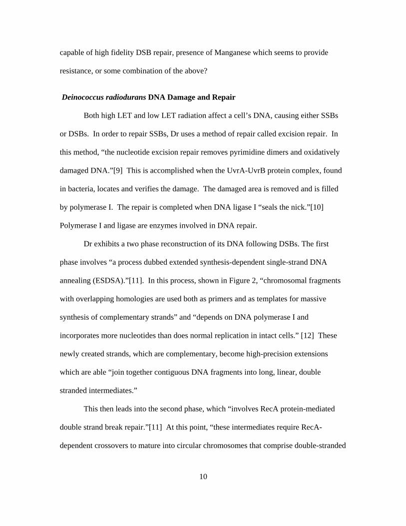
Dr exhibits a two phase reconstruction of its DNA following DSBs. The first
phase involves “a process dubbed extended synthesis-dependent single-strand DNA
annealing (ESDSA).”[11]. In this process, shown in Figure 2, “chromosomal fragments
with overlapping homologies are used both as primers and as templates for massive
synthesis of complementary strands” and “depends on DNA polymerase I and
incorporates more nucleotides than does normal replication in intact cells.” [12] These
newly created strands, which are complementary, become high-precision extensions
which are able “join together contiguous DNA fragments into long, linear, double
stranded intermediates.”
This then leads into the second phase, which “involves RecA protein-mediated
double strand break repair.”[11] At this point, “these intermediates require RecA-
dependent crossovers to mature into circular chromosomes that comprise double-stranded
11
patchworks of numerous DNA blocks synthesized before radiation, connected by DNA
blocks synthesized after radiation.”[12]
Figure 2. Two stages of genome reconstitution in Deinococcus radiodurans.[11]
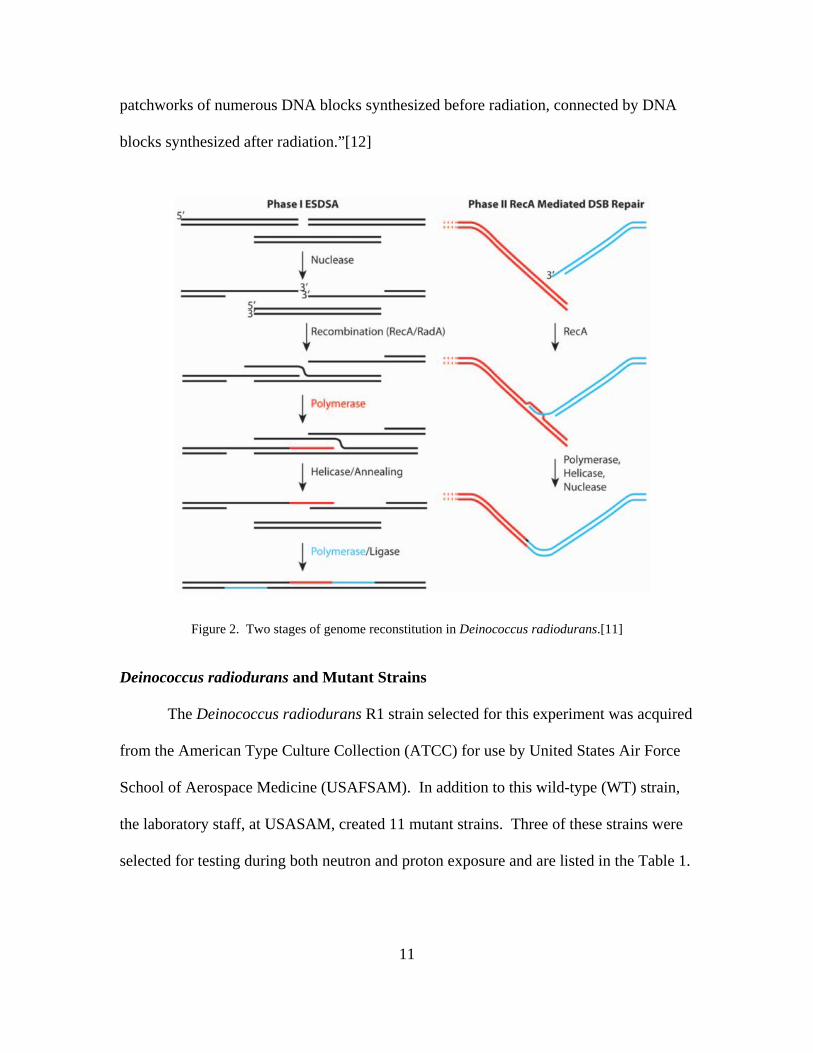
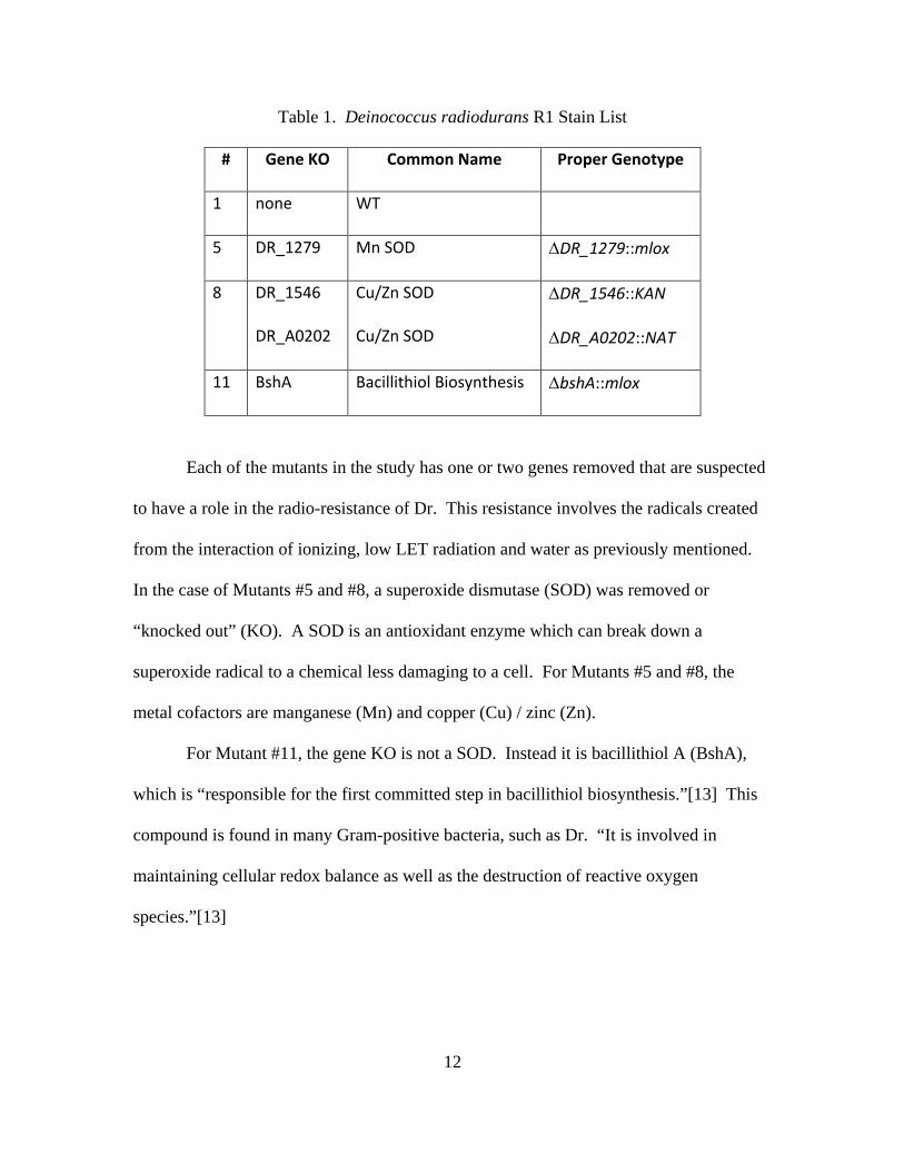
Deinococcus radiodurans and Mutant Strains
The Deinococcus radiodurans R1 strain selected for this experiment was acquired
from the American Type Culture Collection (ATCC) for use by United States Air Force
School of Aerospace Medicine (USAFSAM). In addition to this wild-type (WT) strain,
the laboratory staff, at USASAM, created 11 mutant strains. Three of these strains were
selected for testing during both neutron and proton exposure and are listed in the Table 1.
12
Table 1. Deinococcus radiodurans R1 Stain List
# Gene KO Common Name Proper Genotype
1 none WT
5 DR_1279 Mn SOD ∆DR_1279::mlox
8 DR_1546
DR_A0202
Cu/Zn SOD
Cu/Zn SOD
∆DR_1546::KAN
∆DR_A0202::NAT
11 BshA Bacillithiol Biosynthesis ∆bshA::mlox
Each of the mutants in the study has one or two genes removed that are suspected
to have a role in the radio-resistance of Dr. This resistance involves the radicals created
from the interaction of ionizing, low LET radiation and water as previously mentioned.
In the case of Mutants #5 and #8, a superoxide dismutase (SOD) was removed or
“knocked out” (KO). A SOD is an antioxidant enzyme which can break down a
superoxide radical to a chemical less damaging to a cell. For Mutants #5 and #8, the
metal cofactors are manganese (Mn) and copper (Cu) / zinc (Zn).
For Mutant #11, the gene KO is not a SOD. Instead it is bacillithiol A (BshA),
which is “responsible for the first committed step in bacillithiol biosynthesis.”[13] This
compound is found in many Gram-positive bacteria, such as Dr. “It is involved in
maintaining cellular redox balance as well as the destruction of reactive oxygen
species.”[13]
13
Additionally, a laboratory strain of Escherichia coli (EC), common name DH5A,
acquired from Protein Express, Inc. was used during the 3rd neutron irradiation
experiment.
III. Methodology
Chapter Overview
The purpose of this chapter is to describe the methods used to conduct
experimental procedures on Dr to test the hypothesis listed in the first chapter. This
section begins with how Dr was prepared prior to irradiation. Next, a brief description of
both neutron and proton generation is given. The next subsection looks at irradiation and
rehydration of samples. Finally, an explanation on the methods of statistical analysis is
given.
Deinococcus Radiodurans Sample Preparation
Initial Sample Growth
The bacteria preparation consisted of several steps, ultimately yielding a Dr
sample that was 2-5 x 10⁸ CFU/ml. These steps were conducted at USAFSAM. Initially,
WT and the selected mutants were grown in a tryptone-glucose-yeast extract (TGY, with
antibiotic selection of Nourseothricin (NAT) and Kanamycin (KAN) for mutant #8 only)
culture medium (0.5 % tryptone, 0.3% yeast extract, 0.1% glucose). Colonies were
streaked for isolation and incubated for 48 hours at 32 °C in unsealed plastic bags in
order to prevent drying. After the 48 hours, a single colony per strain was inoculated into
5 ml of TGY culture medium using 14 ml round bottom tubes, again with antibiotics for
14
mutant #8. The inoculated colonies were incubated overnight at 32 °C and 220 RPM for
aeration. The following day, the cultures were diluted 1:100 (200 µl of overnight cell
culture) into 20 ml of fresh TGY culture medium within a 150 ml flask with appropriate
selection of antibiotics for mutant #8. The flasks were incubated overnight at 32 °C and
220 RPM.
After approximately 24 hours, the cultures were diluted to an optical density
(OD600) of 0.25 in 40 ml of TGY culture medium into 250 ml flasks. This was achieved
using the Thermo Scientific NanoDrop 2000c Spectrophotometer and accompanying
software. A 1:10 dilution sample of each Dr strain (100 µl of culture, 900 µl TGY) was
added to a cuvette. The NanoDrop 2000c then took readings based on a 10mm
pathlength of light. Below is a sample calculation showing how much culture needed to
be added to achieve the OD600 of 0.25. The initial OD600 was multiplied by 10 to account
for a 1:10 dilution. Tables of these measurements for each experiment appear in
Appendix A.
40 𝑚𝑚𝑚𝑚 ∗ . 254.97
= 2.0 𝑚𝑚𝑚𝑚
The flasks were then incubated four hours at 32 °C and 220 RPM to achieve early log
phase.
After the incubation period was completed, the cultures were concentrated 10x by
centrifugation, with 30 ml of the cultures transferred into 50 ml conical tubes, set to 3500
RPM for 20 minutes in a table top centrifuge. During the spin, OD600 readings were
taken to determine the CFU/ml post four hour incubation. A calculation was done to
15
determine the amount of media to achieve an OD600 of 5. Tables of these calculations are
found in Appendix A.
30 𝑚𝑚𝑚𝑚 ∗ . 624
5= 3.7 𝑚𝑚𝑚𝑚
Next, the supernatant was poured off completely and the remaining pellets were re-
suspended into fresh TGY culture media to achieve an OD600 of 5, which corresponds to
2-5 x 10⁸ CFU/ml.
Sample Plate Preparation
In a biosafety cabinet, the samples were transferred to the wells of a 96 well plate
column in order to easily deposit the samples onto the 96 well, flat bottom plate lids. The
procedure was utilized for the first and second neutron experiments.
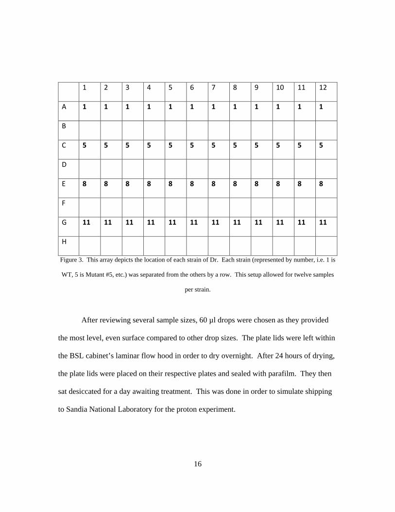
Using a multi-channel pipet, 60 µl of cells were transferred to the lid “wells” of
three 96 well, flat bottom plate lids as shown in Figure 3. One plate lid was used as an
untreated control, while the other two plate lids were irradiated. The lid wells were used
instead of the actual wells because of the follow on experiments. Specifically, at Sandia
National Lab using the QASPR-3 (Qualification Alternative to the Sandia Pulse Reactor
3) tandem ion beam, only a 96 well plate lid, not the plate, was initially thought to fit the
sample stage in the QASPR-3’s irradiation chamber, so all experimentation was
completed using the lid wells.
16
1 2 3 4 5 6 7 8 9 10 11 12
A 1 1 1 1 1 1 1 1 1 1 1 1
B
C 5 5 5 5 5 5 5 5 5 5 5 5
D
E 8 8 8 8 8 8 8 8 8 8 8 8
F
G 11 11 11 11 11 11 11 11 11 11 11 11
H
Figure 3. This array depicts the location of each strain of Dr. Each strain (represented by number, i.e. 1 is
WT, 5 is Mutant #5, etc.) was separated from the others by a row. This setup allowed for twelve samples
per strain.
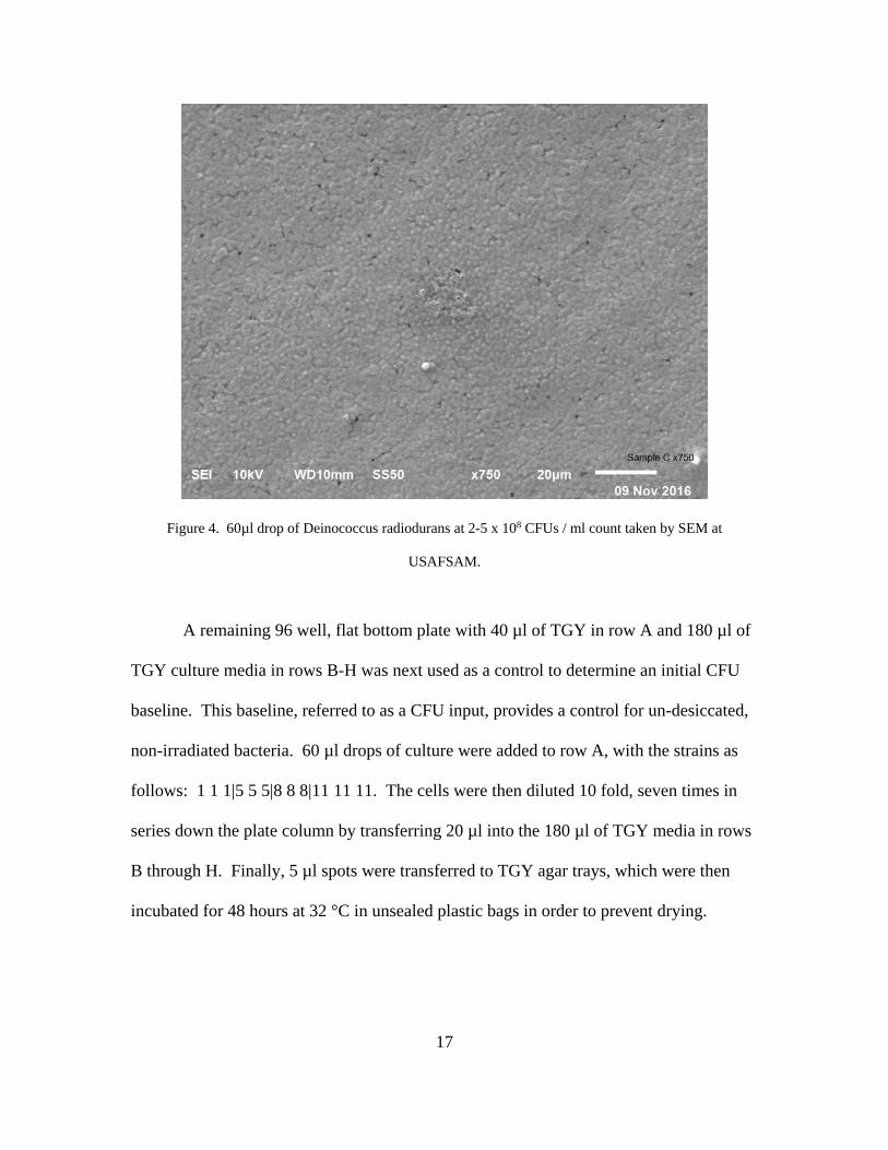
After reviewing several sample sizes, 60 µl drops were chosen as they provided
the most level, even surface compared to other drop sizes. The plate lids were left within
the BSL cabinet’s laminar flow hood in order to dry overnight. After 24 hours of drying,
the plate lids were placed on their respective plates and sealed with parafilm. They then
sat desiccated for a day awaiting treatment. This was done in order to simulate shipping
to Sandia National Laboratory for the proton experiment.
17
Figure 4. 60µl drop of Deinococcus radiodurans at 2-5 x 10⁸ CFUs / ml count taken by SEM at
USAFSAM.
A remaining 96 well, flat bottom plate with 40 µl of TGY in row A and 180 µl of
TGY culture media in rows B-H was next used as a control to determine an initial CFU
baseline. This baseline, referred to as a CFU input, provides a control for un-desiccated,
non-irradiated bacteria. 60 µl drops of culture were added to row A, with the strains as
follows: 1 1 1|5 5 5|8 8 8|11 11 11. The cells were then diluted 10 fold, seven times in
series down the plate column by transferring 20 µl into the 180 µl of TGY media in rows
B through H. Finally, 5 µl spots were transferred to TGY agar trays, which were then
incubated for 48 hours at 32 °C in unsealed plastic bags in order to prevent drying.
18
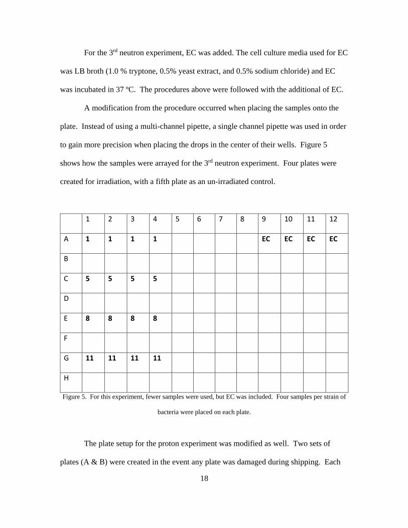
For the 3rd neutron experiment, EC was added. The cell culture media used for EC
was LB broth (1.0 % tryptone, 0.5% yeast extract, and 0.5% sodium chloride) and EC
was incubated in 37 ºC. The procedures above were followed with the additional of EC.
A modification from the procedure occurred when placing the samples onto the
plate. Instead of using a multi-channel pipette, a single channel pipette was used in order
to gain more precision when placing the drops in the center of their wells. Figure 5
shows how the samples were arrayed for the 3rd neutron experiment. Four plates were
created for irradiation, with a fifth plate as an un-irradiated control.
1 2 3 4 5 6 7 8 9 10 11 12
A 1 1 1 1 EC EC EC EC
B
C 5 5 5 5
D
E 8 8 8 8
F
G 11 11 11 11
H
Figure 5. For this experiment, fewer samples were used, but EC was included. Four samples per strain of
bacteria were placed on each plate.
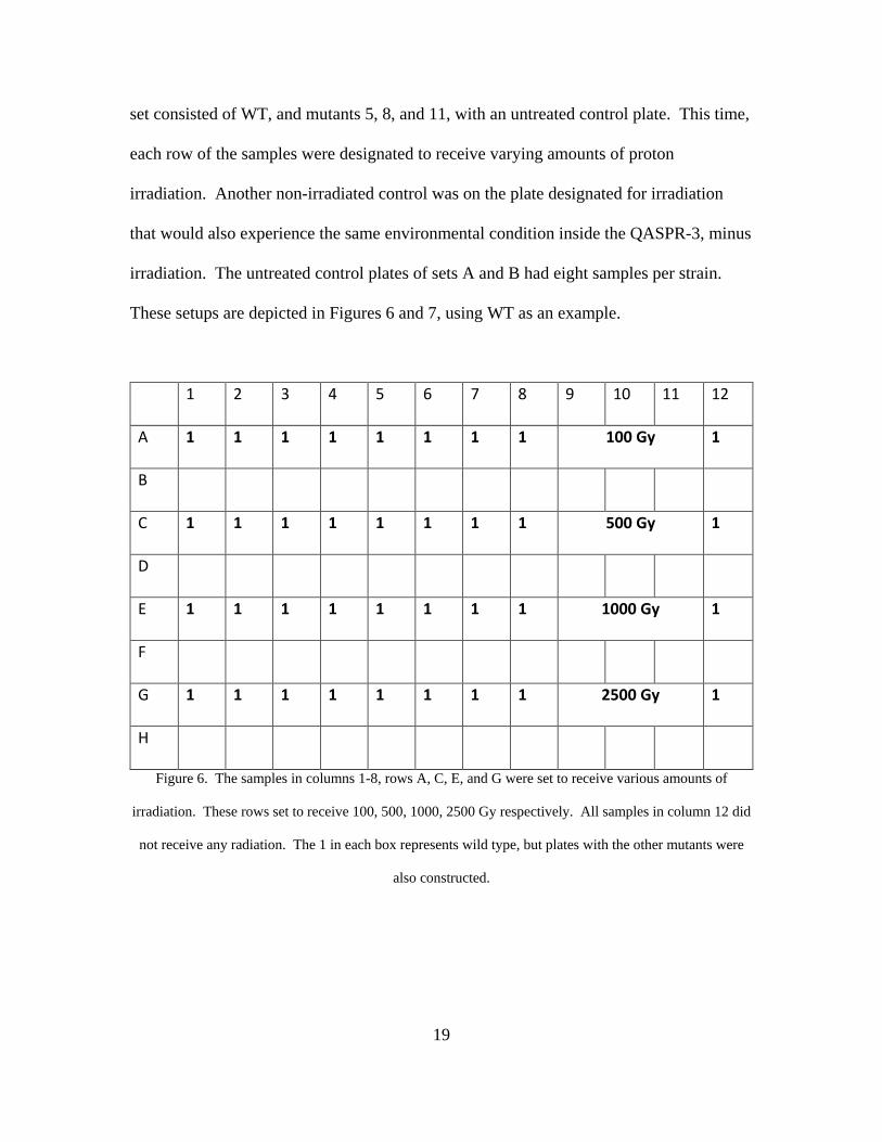
The plate setup for the proton experiment was modified as well. Two sets of
plates (A & B) were created in the event any plate was damaged during shipping. Each
19
set consisted of WT, and mutants 5, 8, and 11, with an untreated control plate. This time,
each row of the samples were designated to receive varying amounts of proton
irradiation. Another non-irradiated control was on the plate designated for irradiation
that would also experience the same environmental condition inside the QASPR-3, minus
irradiation. The untreated control plates of sets A and B had eight samples per strain.
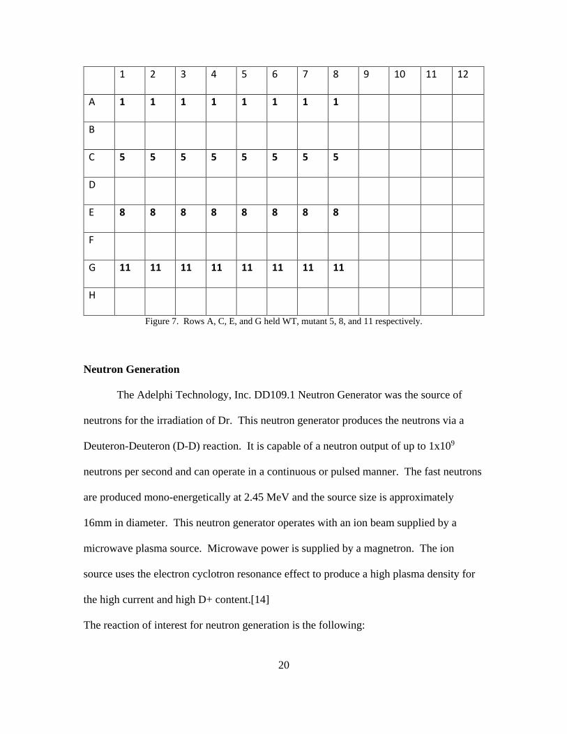
These setups are depicted in Figures 6 and 7, using WT as an example.
1 2 3 4 5 6 7 8 9 10 11 12
A 1 1 1 1 1 1 1 1 100 Gy 1
B
C 1 1 1 1 1 1 1 1 500 Gy 1
D
E 1 1 1 1 1 1 1 1 1000 Gy 1
F
G 1 1 1 1 1 1 1 1 2500 Gy 1
H
Figure 6. The samples in columns 1-8, rows A, C, E, and G were set to receive various amounts of
irradiation. These rows set to receive 100, 500, 1000, 2500 Gy respectively. All samples in column 12 did
not receive any radiation. The 1 in each box represents wild type, but plates with the other mutants were
also constructed.
20
1 2 3 4 5 6 7 8 9 10 11 12
A 1 1 1 1 1 1 1 1
B
C 5 5 5 5 5 5 5 5
D
E 8 8 8 8 8 8 8 8
F
G 11 11 11 11 11 11 11 11
H
Figure 7. Rows A, C, E, and G held WT, mutant 5, 8, and 11 respectively.
Neutron Generation
The Adelphi Technology, Inc. DD109.1 Neutron Generator was the source of
neutrons for the irradiation of Dr. This neutron generator produces the neutrons via a
Deuteron-Deuteron (D-D) reaction. It is capable of a neutron output of up to 1x10⁹
neutrons per second and can operate in a continuous or pulsed manner. The fast neutrons
are produced mono-energetically at 2.45 MeV and the source size is approximately
16mm in diameter. This neutron generator operates with an ion beam supplied by a
microwave plasma source. Microwave power is supplied by a magnetron. The ion
source uses the electron cyclotron resonance effect to produce a high plasma density for
the high current and high D+ content.[14]
The reaction of interest for neutron generation is the following:
21
2D + 2D → 3He (0.87 MeV) + n (2.45 MeV)
The generator is able to do this by using a titanium hydride target, which is
impregnated with deuterium atoms. Deuterium gas is injected into the plasma chamber,
which is ionized by the microwave source. A sufficient voltage, which overcomes the
Coulomb barrier, is applied between the ion chamber and target. This accelerates the
deuterium ions to the target, enabling them to fuse with the deuterons in the titanium.
The products of this fusion are the 2.45 MeV neutrons and He. However, this reaction
only occurs 50% of the time. The other 50% of the time the following reaction occurs
[15]:
2D + 2D → T + H
Neutron Dose Calculations
In order to calculate the dose of radiation via neutron exposures, the method as
outlined by Cember in Introduction to Health Physics was followed. [16] Using N, the
number of atoms/kg, f, the mean fractional energy transferred from neutron to scattered
atom during collision with the neutron, and σ, the scattering cross section of the element
for neutrons of energy E (2.45 MeV), the following value was found, as shown in Table
2.
22
Table 2. Deinococcus radiodurans Cell Composition
Element
% Mass
N,
atoms/kg f σ, cm2 Nσf
Oxygen 0.13 2.69E+25 0.111 8.45410E-25 2.524E+00
Carbon 0.31 6.41E+24 0.142 1.58290E-24 1.441E+00
Hydrogen 0.49 5.98E+25 0.5 2.59131E-24 7.748E+01
Nitrogen 0.07 1.49E+24 0.124 1.30501E-24 2.411E-01
Σ Nσf 8.169E+01 cm2/kg
The following references apply to the values on this table: % Mass[17], N [16], f[16], and σ[18]
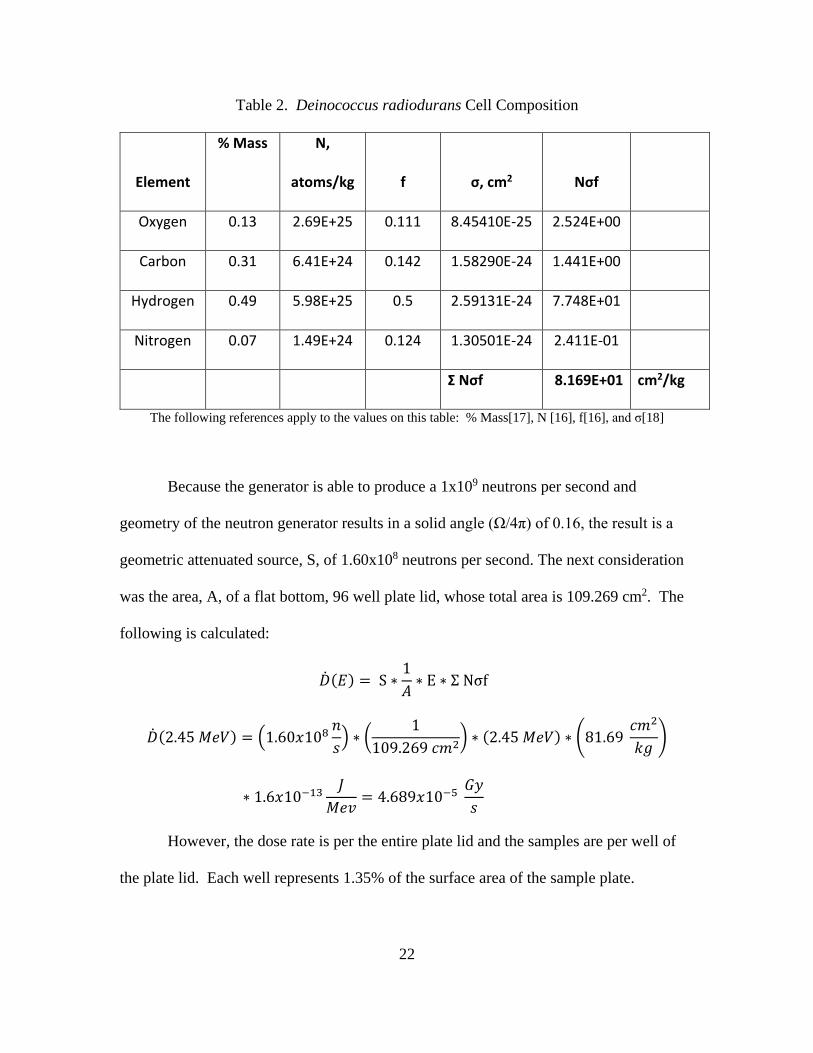
Because the generator is able to produce a 1x10⁹ neutrons per second and
geometry of the neutron generator results in a solid angle (Ω/4π) of 0.16, the result is a
geometric attenuated source, S, of 1.60x10⁸ neutrons per second. The next consideration
was the area, A, of a flat bottom, 96 well plate lid, whose total area is 109.269 cm2. The
following is calculated:
�̇�𝐷(𝐸𝐸) = S ∗1𝐴𝐴∗ E ∗ Σ Nσf
�̇�𝐷(2.45 𝑀𝑀𝑀𝑀𝑀𝑀) = �1.60𝑥𝑥108𝑛𝑛𝑠𝑠� ∗ �
1109.269 𝑐𝑐𝑚𝑚2� ∗ (2.45 𝑀𝑀𝑀𝑀𝑀𝑀) ∗ �81.69
𝑐𝑐𝑚𝑚2
𝑘𝑘𝑘𝑘�
∗ 1.6𝑥𝑥10−13𝐽𝐽
𝑀𝑀𝑀𝑀𝑀𝑀= 4.689𝑥𝑥10−5
𝐺𝐺𝐺𝐺𝑠𝑠
However, the dose rate is per the entire plate lid and the samples are per well of
the plate lid. Each well represents 1.35% of the surface area of the sample plate.
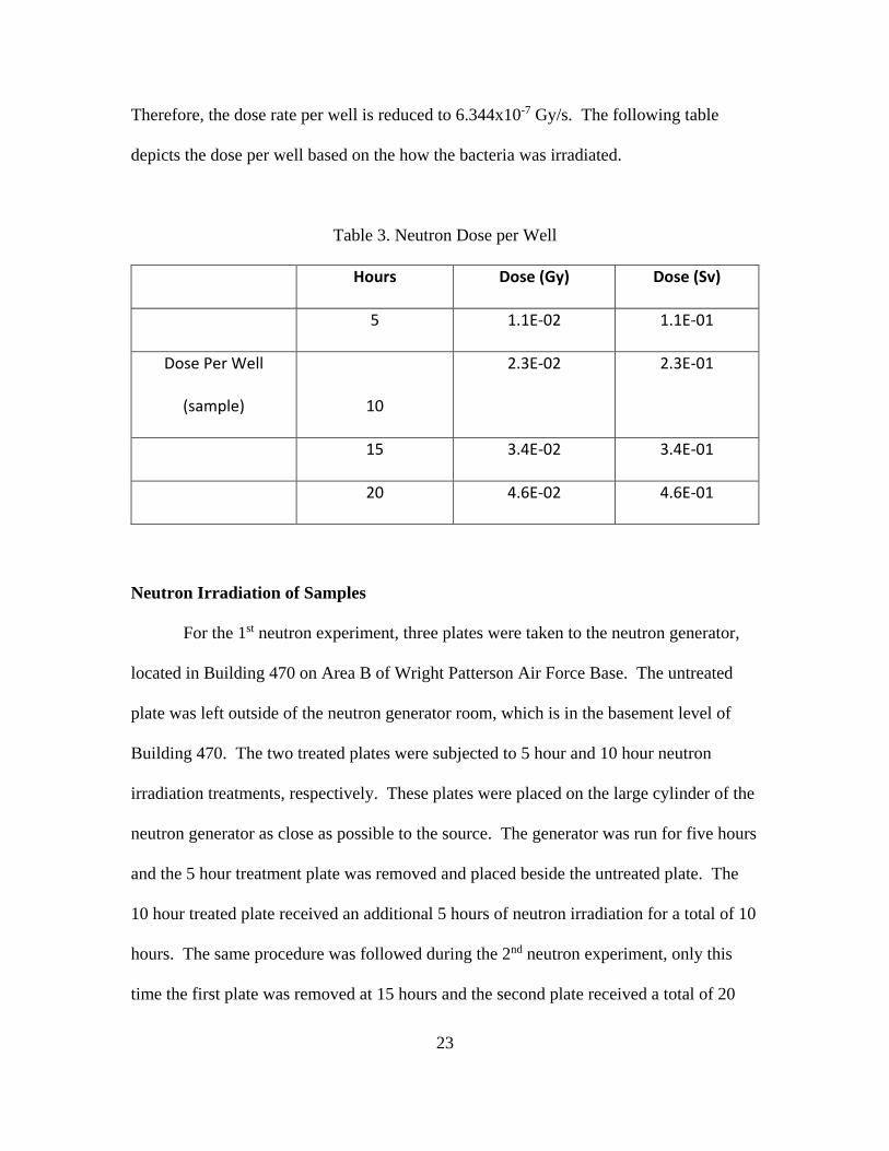
23
Therefore, the dose rate per well is reduced to 6.344x10⁻⁷ Gy/s. The following table
depicts the dose per well based on the how the bacteria was irradiated.
Table 3. Neutron Dose per Well
Hours Dose (Gy) Dose (Sv)
5 1.1E-02 1.1E-01
Dose Per Well
(sample) 10
2.3E-02 2.3E-01
15 3.4E-02 3.4E-01
20 4.6E-02 4.6E-01
Neutron Irradiation of Samples
For the 1st neutron experiment, three plates were taken to the neutron generator,
located in Building 470 on Area B of Wright Patterson Air Force Base. The untreated
plate was left outside of the neutron generator room, which is in the basement level of
Building 470. The two treated plates were subjected to 5 hour and 10 hour neutron
irradiation treatments, respectively. These plates were placed on the large cylinder of the
neutron generator as close as possible to the source. The generator was run for five hours
and the 5 hour treatment plate was removed and placed beside the untreated plate. The
10 hour treated plate received an additional 5 hours of neutron irradiation for a total of 10
hours. The same procedure was followed during the 2nd neutron experiment, only this
time the first plate was removed at 15 hours and the second plate received a total of 20
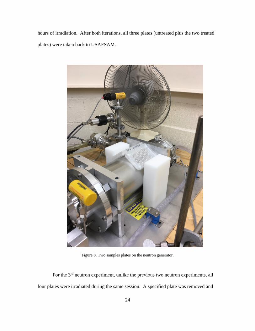
24
hours of irradiation. After both iterations, all three plates (untreated plus the two treated
plates) were taken back to USAFSAM.
Figure 8. Two samples plates on the neutron generator.
For the 3rd neutron experiment, unlike the previous two neutron experiments, all
four plates were irradiated during the same session. A specified plate was removed and
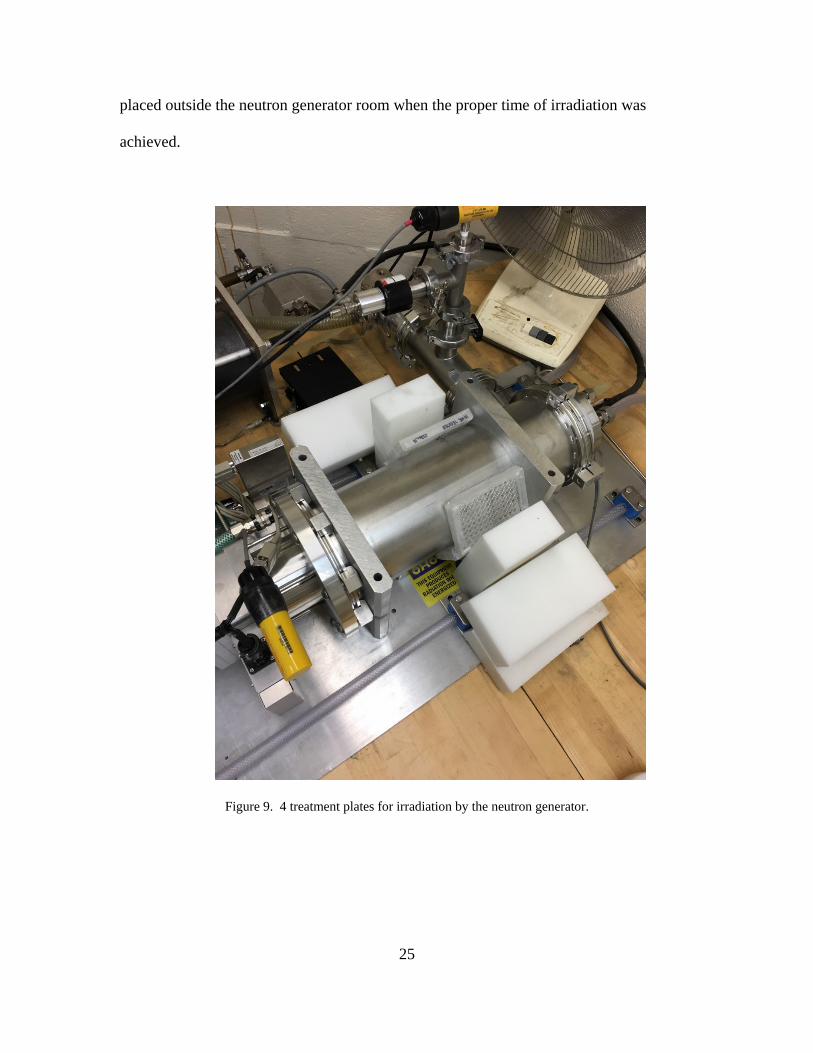
25
placed outside the neutron generator room when the proper time of irradiation was
achieved.
Figure 9. 4 treatment plates for irradiation by the neutron generator.
26
Rehydration of Samples and Spotting Post Neutron Irradiation
After an approximate 24 hour waiting period to again to simulate shipping
conditions, all three sample plates for the first and second neutron experiments were
rehydrated with 60 µl of fresh TGY medium. The medium was pipetted up and down 20
times to re-suspend the cells. Next, the re-hydrated cells were pipetted up and down an
additional 20 times to further re-suspend then transferred to a new 96 well, flat bottom
plate. Another 40 µl of fresh TGY culture medium was added for a total of 100 µl of cell
culture. The bacteria were then diluted 10 fold, seven times in series by transferring 20
µl in the 180 µl of TGY media. Finally, 5 µl spots were transferred to TGY agar trays,
which were then incubated for 48 hours at 32 °C in unsealed plastic bags in order to
prevent drying. The resulting colonies were then counted. This was the same serial
dilution procedure as previously mentioned for the CFU input control.
In the case of the 3rd neutron experiment, a modification involved the re-hydration
of the cells. The cells were diluted 10 fold, seven times in series down the plate column
as previously mentioned. However, the additional 40 µl of TGY was not added to the 60
µl rehydrated spots in row A of the column well plate this time, resulting in all counts
conducted at the 10-5, not 10-4 dilution. Next, EC was spotted in 5 µl spots on LB agar,
incubated for 24 hours, then the resulting colonies were counted. In addition to the 5 µl
spots, 100 µl of Dr was spread on round TGY plates. This was done in order to decrease
the variability of the experiment if possible. These trays were incubated for 48 hours.
27
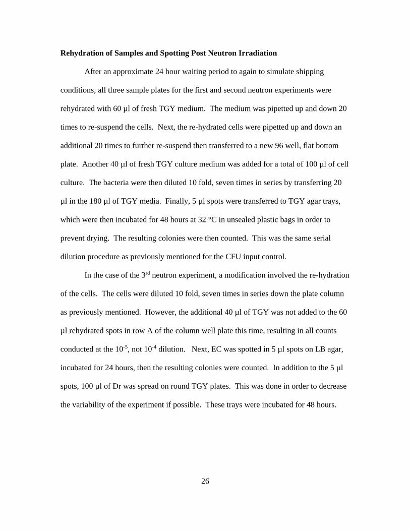
Colony Counting Post Neutron Irradiation
After the 48 hour incubation period, cell colonies were counted at the 4th dilution
of each sample tray for the first and second neutron experiment. The cells were counted
via visual inspection. The number of colonies per each sample was then recorded.
Following the 3rd neutron experiment, the 100 µl spread plates were counted and
recorded.
Figure 10. Wild Type Deinococcus radiodurans following a five hour neutron treatment in the 1st Neutron
experiment.
28
Proton Generation
The protons used for irradiation of Dr samples were generated by one of the
Sandia National Laboratory’s ion beams, QASPR-3. This device is a located at the
Sandia National Laboratory’s Ion Beam Lab located on Kirtland Air Force Base, New
Mexico. This lab was opened in 2010 and is a “state-of-the-art facility using ion and
electron accelerators to study and modify materials.”[19] The QASPR-3 is a HVE 6 MV
Tandem ion accelerator which “can accelerate most elements from hydrogen to gold. It
is used for in-situ electrical testing, optical testing, and mechanical testing to determine
the response of materials to radiation damage at various temperatures from -230 ºC to
1200 ºC. There is also a microbeam with a spot size of approximately 1 µm.” [19] In
the case of this experiment, the ion beam was used as proton radiation source.
Proton Dose Calculations
As mentioned earlier, a 60 μl drop, desiccated, is the target layer for the beam.
Since the cells are spherical, ranging from 1.5 to 3.5 μm in diameter, an average diameter
of 2.5 μm and an average radius is 1.25 μm was used for calculations. The 60 μl drop is
taken from concentration of 2-5x10⁸ CFU/ml. Again, taking the average, the concentration
is 3.5x10⁸ CFU/ml.
60 𝜇𝜇𝑚𝑚 ∗ 1 𝑚𝑚𝑚𝑚
1000 𝜇𝜇𝑚𝑚 ∗ 3.5 𝑥𝑥 108
𝐶𝐶𝐶𝐶𝐶𝐶𝑚𝑚𝑚𝑚
= 2.1 𝑥𝑥 107𝐶𝐶𝐶𝐶𝐶𝐶
So, in a 60 µl drop, it is expected to have 2.1 x 10⁷ CFUs. Based on the average
size and shape of Dr, the volume Dr in the drop is determined by the following:
𝑀𝑀𝑉𝑉𝑚𝑚𝑉𝑉𝑚𝑚𝑀𝑀 𝑉𝑉𝑜𝑜 𝐷𝐷𝐷𝐷 = 43∗ 𝜋𝜋 ∗ (1.25 𝑥𝑥 10−6𝑚𝑚)3 ∗ 4 ∗ 2.1𝑥𝑥107 = 6.87 𝑥𝑥 10−10 𝑚𝑚3
29
Assuming, at most, the layer will take up the entire lid plate well, whose area is
3.165 x 10⁻⁵ m2, the layer depth is demonstrated via the follow equation:
𝐿𝐿𝐿𝐿𝐺𝐺𝑀𝑀𝐷𝐷 𝐷𝐷𝑀𝑀𝐷𝐷𝐷𝐷ℎ 𝑉𝑉𝑜𝑜 𝐷𝐷𝐷𝐷 = 𝑀𝑀𝑉𝑉𝑚𝑚𝑉𝑉𝑚𝑚𝑀𝑀 𝑉𝑉𝑜𝑜 𝐷𝐷𝐷𝐷
3.165 𝑥𝑥 10−5 𝑚𝑚2 = 0.0000217 𝑚𝑚
This means that the 60 µl drop as a layer depth of 21.7 µm. The polystyrene plate lid has a
thickness of 1.27 mm. The density of Dr is 0.9392 g/cm3. [17]
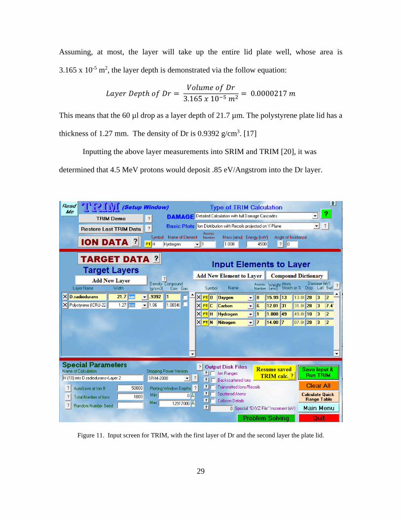
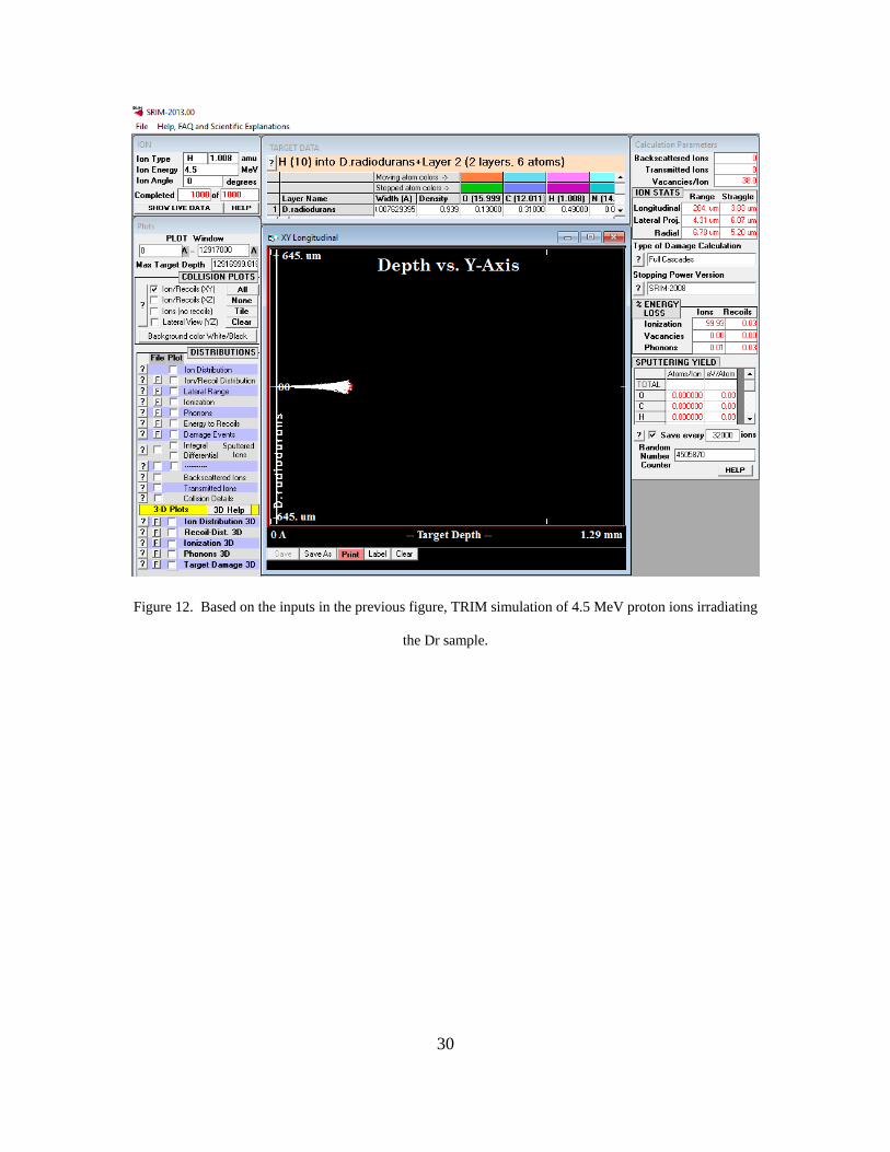
Inputting the above layer measurements into SRIM and TRIM [20], it was
determined that 4.5 MeV protons would deposit .85 eV/Angstrom into the Dr layer.
Figure 11. Input screen for TRIM, with the first layer of Dr and the second layer the plate lid.
30
Figure 12. Based on the inputs in the previous figure, TRIM simulation of 4.5 MeV proton ions irradiating
the Dr sample.
31
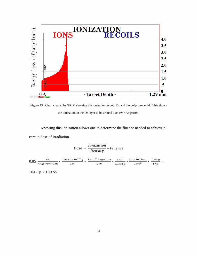
Figure 13. Chart created by TRIM showing the ionization in both Dr and the polystyrene lid. This shows
the ionization in the Dr layer to be around 0.85 eV / Angstrom.
Knowing this ionization allows one to determine the fluence needed to achieve a
certain dose of irradiation.
𝐷𝐷𝑉𝑉𝑠𝑠𝑀𝑀 = 𝐼𝐼𝑉𝑉𝑛𝑛𝐼𝐼𝐼𝐼𝐿𝐿𝐷𝐷𝐼𝐼𝑉𝑉𝑛𝑛𝐷𝐷𝑀𝑀𝑛𝑛𝑠𝑠𝐼𝐼𝐷𝐷𝐺𝐺
∗ 𝐶𝐶𝑚𝑚𝑉𝑉𝑀𝑀𝑛𝑛𝑐𝑐𝑀𝑀
0.85 𝑒𝑒𝑒𝑒𝐴𝐴𝐴𝐴𝐴𝐴𝐴𝐴𝐴𝐴𝐴𝐴𝐴𝐴𝐴𝐴−𝐼𝐼𝐴𝐴𝐴𝐴
∗ 1.6022 𝑥𝑥 10−19 𝐽𝐽1 𝑒𝑒𝑒𝑒
∗ 1 𝑥𝑥 108 𝐴𝐴𝐴𝐴𝐴𝐴𝐴𝐴𝐴𝐴𝐴𝐴𝐴𝐴𝐴𝐴1 𝑐𝑐𝐴𝐴
∗ 𝑐𝑐𝐴𝐴3
0.9392 𝐴𝐴∗ 7.2 𝑥𝑥 109 𝐼𝐼𝐴𝐴𝐴𝐴𝐴𝐴
1 𝑐𝑐𝐴𝐴2 ∗ 1000 𝐴𝐴1 𝑘𝑘𝐴𝐴
=
104 𝐺𝐺𝐺𝐺 ~ 100 𝐺𝐺𝐺𝐺
32
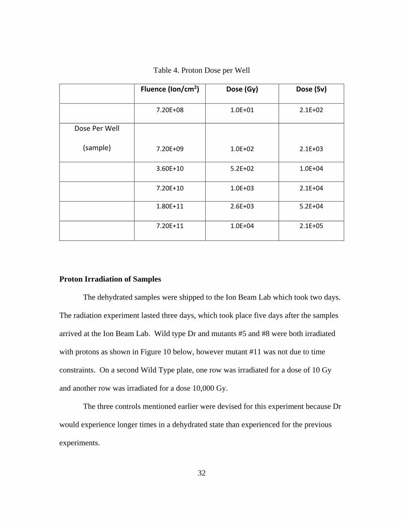
Table 4. Proton Dose per Well
Fluence (Ion/cm2) Dose (Gy) Dose (Sv)
7.20E+08 1.0E+01 2.1E+02
Dose Per Well
(sample) 7.20E+09 1.0E+02 2.1E+03
3.60E+10 5.2E+02 1.0E+04
7.20E+10 1.0E+03 2.1E+04
1.80E+11 2.6E+03 5.2E+04
7.20E+11 1.0E+04 2.1E+05
Proton Irradiation of Samples
The dehydrated samples were shipped to the Ion Beam Lab which took two days.
The radiation experiment lasted three days, which took place five days after the samples
arrived at the Ion Beam Lab. Wild type Dr and mutants #5 and #8 were both irradiated
with protons as shown in Figure 10 below, however mutant #11 was not due to time
constraints. On a second Wild Type plate, one row was irradiated for a dose of 10 Gy
and another row was irradiated for a dose 10,000 Gy.
The three controls mentioned earlier were devised for this experiment because Dr
would experience longer times in a dehydrated state than experienced for the previous
experiments.
33
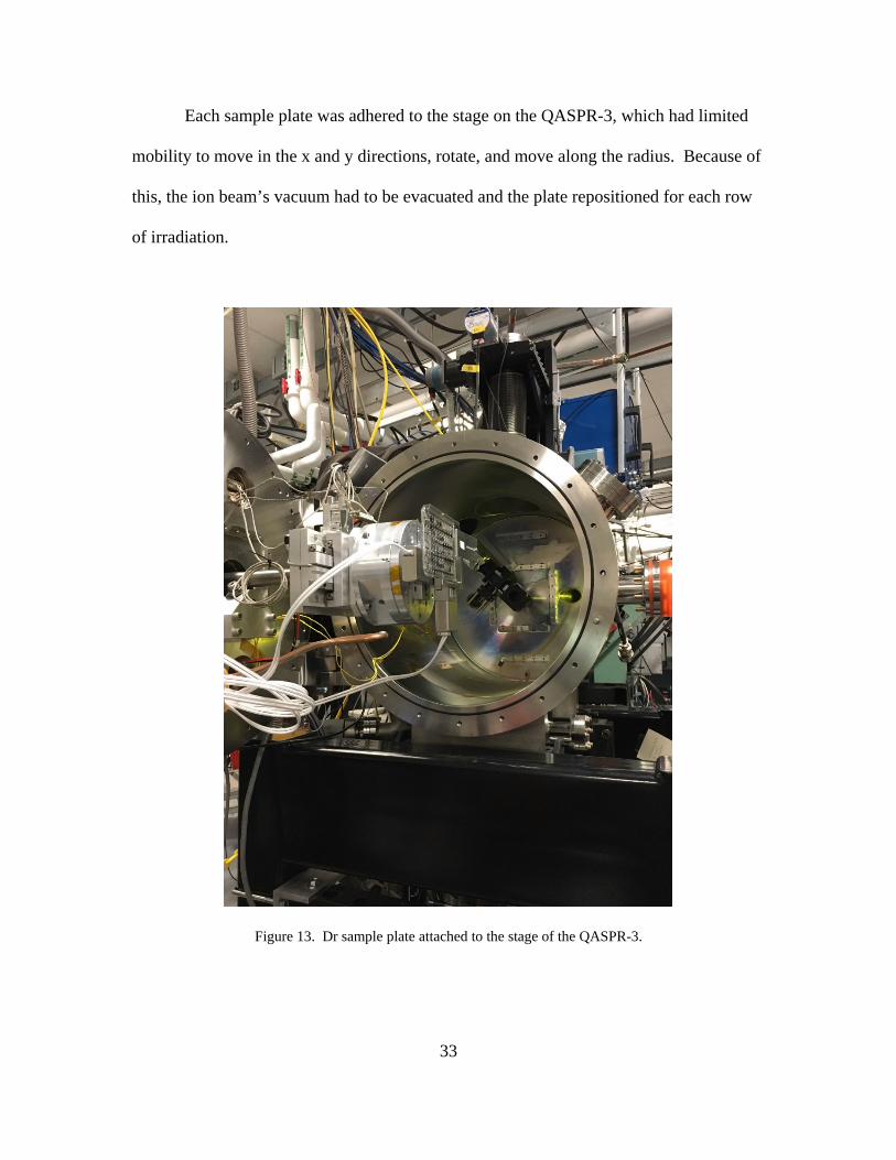
Each sample plate was adhered to the stage on the QASPR-3, which had limited
mobility to move in the x and y directions, rotate, and move along the radius. Because of
this, the ion beam’s vacuum had to be evacuated and the plate repositioned for each row
of irradiation.
Figure 13. Dr sample plate attached to the stage of the QASPR-3.
34
Figure 14. The QASPR-3 proton beam was able to hit the total area each well by firing shots in a grid
pattern based on the area of the beam. Top Row: Shots 1-4; Center Row: Shots 5-8; Bottom Row: Shots
9-12.
At the beginning of each day of experimentation the beams conditions such as the
beam current and area were validated. The beam itself was calibrated using a phosphorus
target situated on the stage above the sample lid as shown in Figure 13. This enabled the
operator of the beam to both validate the fluence in ions/cm2 and the beam’s width, which
would determine the grid pattern of shots, such in Figure 14. The ion beam’s fluence was
always within ten percent of the requested fluence. The QASPR-3 was able to accelerate
the protons in a directed beam so that the entire well was evenly covered with no overlap,
with an example of a well in Figure 14. The samples were shipped the next day
following the end of the experiment and arrived back at USAFSAM two days later.
35
Rehydration of Samples and Spotting Post Proton Irradiation
After arriving back at USAFAM, the samples were rehydrated five days later.
The process was similar to the rehydration of samples following the neutron experiments.
All irradiated sample and control plates were rehydrated with 60 µl of fresh TGY
medium. The medium was pipetted up and down 20 times to re-suspend the cells. Next,
the re-hydrated cells were pipetted up and down an additional 20 times to further re-
suspend then transferred to a new 96 well, flat bottom plate. The bacteria were then
diluted 10 fold, seven times in series by transferring 20 µl in the 180 µl of TGY media.
Finally, 5 µl spots were transferred to TGY agar trays, which were then incubated for 48
hours at 32 °C in unsealed plastic bags in order to prevent drying. The resulting colonies
were then counted.
Colony Counting Post Proton Irradiation
After a 72 hour incubation period, cell colonies were counted at the 5th dilution of
each sample tray for the proton experiment. The cells were counted via visual inspection.
The number of colonies per each sample was then recorded.
36
Figure 15. Wild Type Dr re-growth after 500 Gy irradiation. Colonies were counted at the 10-5 dilution.
Statistical Methods of Comparison
A statistical analysis was conducted between the following samples - CFU input
control to non-irradiated control, and non-irradiated control to the irradiated sample
populations. The statistical analysis consisted of a small, independent sample test of
hypothesis for a population, µ1, to another population, µ2, using the Student’s t-
Statistic.[21] This method was chosen because of the small sample size (< 30 samples),
with the following assumptions: 1 – the two samples are randomly selected in an
independent manner from the two target populations, 2 – both samples’ populations have
37
distributions that are approximately normal, and 3 – the population variances are equal.
Due to this, a pooled sample estimator, sp2, was used. This was calculated the following
way:
𝑠𝑠𝑝𝑝2 = (𝑛𝑛1 − 1)𝑠𝑠12 + (𝑛𝑛2 − 1)𝑠𝑠22
𝑛𝑛1 + 𝑛𝑛2 − 2
where n is the number of samples per strain irradiation treatment and s2 is the sample
variance.
The populations were then compared using a one-tailed test, with the subsequent
equations showing the null hypothesis, H0, the alternate hypothesis, Ha, the test statistic, t,
each samples mean colony counts, x-bar1 and x-bar2, and the rejection region, ta, which is
based on (n1 + n2 – 2) degrees of freedom. The variable, a, was 0.05 to reflect a 95 %
confidence.[21]
𝐻𝐻0: (𝜇𝜇1 − 𝜇𝜇1) = 0
𝐻𝐻𝑎𝑎: (𝜇𝜇1 − 𝜇𝜇1) > 0
𝐷𝐷 =( 𝑥𝑥1 − 𝑥𝑥2 )
�𝑠𝑠𝑝𝑝2( 1𝑛𝑛1
+ 1𝑛𝑛2
)
𝑅𝑅𝑀𝑀𝑅𝑅𝑀𝑀𝑐𝑐𝐷𝐷𝐼𝐼𝑉𝑉𝑛𝑛 𝑅𝑅𝑀𝑀𝑘𝑘𝐼𝐼𝑉𝑉𝑛𝑛: 𝐷𝐷 > 𝐷𝐷𝑎𝑎
IV. Analysis and Results
Chapter Overview
The purpose of this chapter is to review the statistical analysis conducted between
the irradiated sample colonies and their controls. All populations were compared with
95% certainty. The comparisons are broken down by experiment, with only the cases of
38
statistical difference or close to statistical difference appearing the Tables 5 - 8. Close to
statistical difference is defined as a difference of 0.1 or less between the t-statistics and
the rejection region.
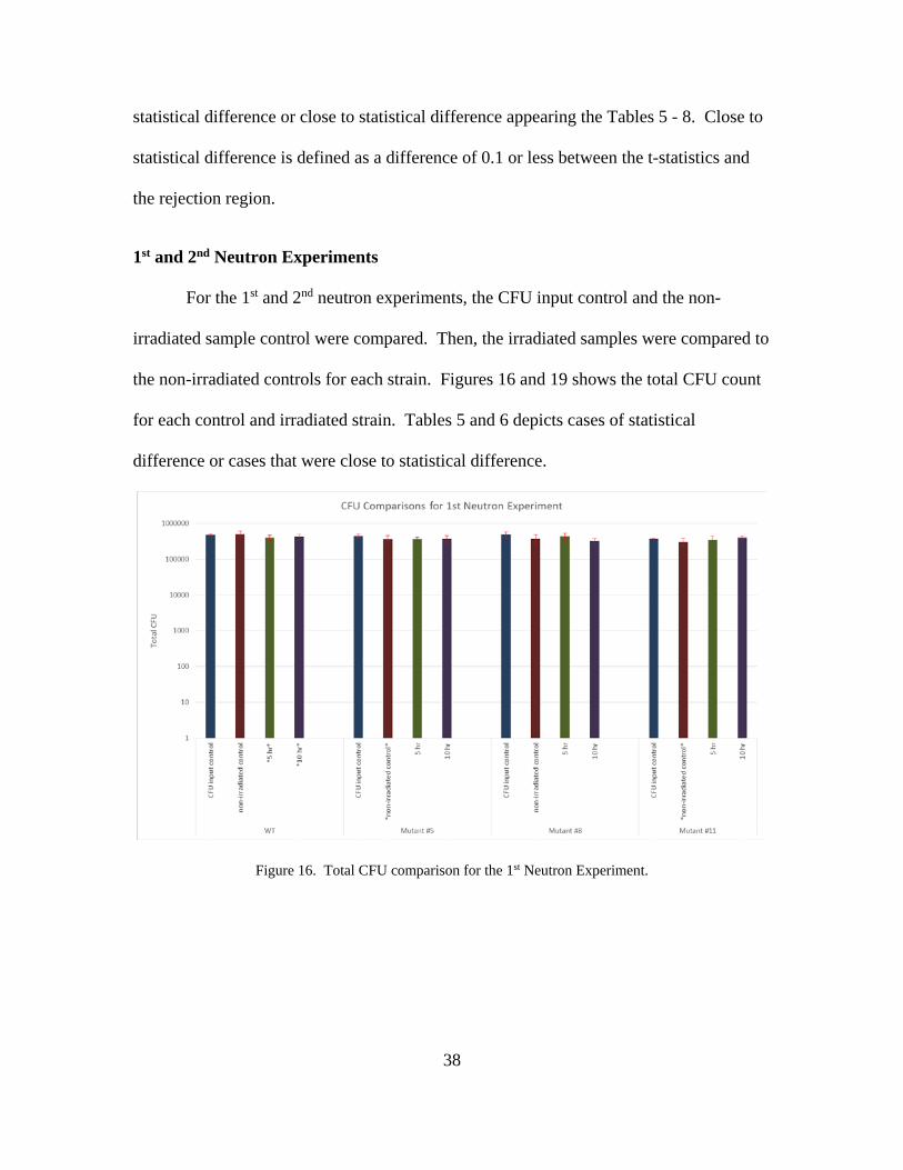
1st and 2nd Neutron Experiments
For the 1st and 2nd neutron experiments, the CFU input control and the non-
irradiated sample control were compared. Then, the irradiated samples were compared to
the non-irradiated controls for each strain. Figures 16 and 19 shows the total CFU count
for each control and irradiated strain. Tables 5 and 6 depicts cases of statistical
difference or cases that were close to statistical difference.
Figure 16. Total CFU comparison for the 1st Neutron Experiment.
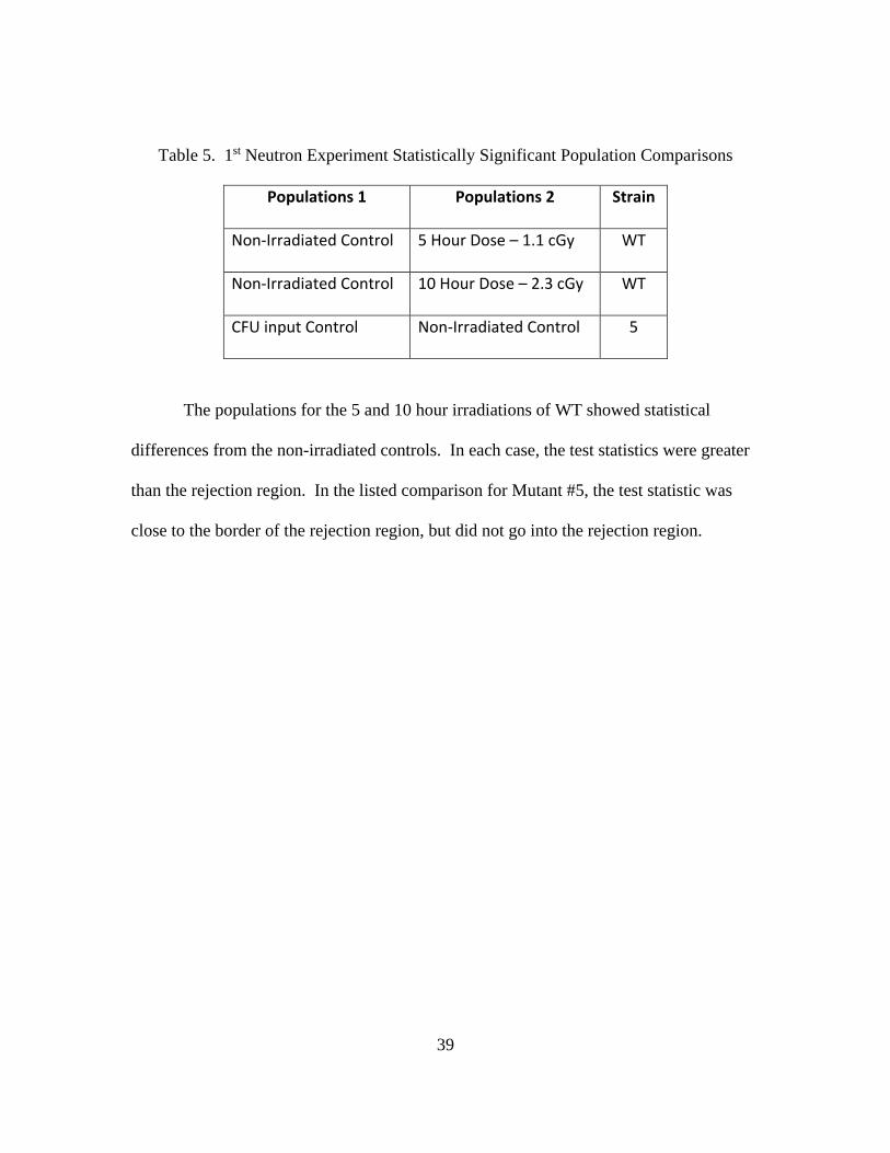
39
Table 5. 1st Neutron Experiment Statistically Significant Population Comparisons
Populations 1 Populations 2 Strain
Non-Irradiated Control 5 Hour Dose – 1.1 cGy WT
Non-Irradiated Control 10 Hour Dose – 2.3 cGy WT
CFU input Control Non-Irradiated Control 5
The populations for the 5 and 10 hour irradiations of WT showed statistical
differences from the non-irradiated controls. In each case, the test statistics were greater
than the rejection region. In the listed comparison for Mutant #5, the test statistic was
close to the border of the rejection region, but did not go into the rejection region.
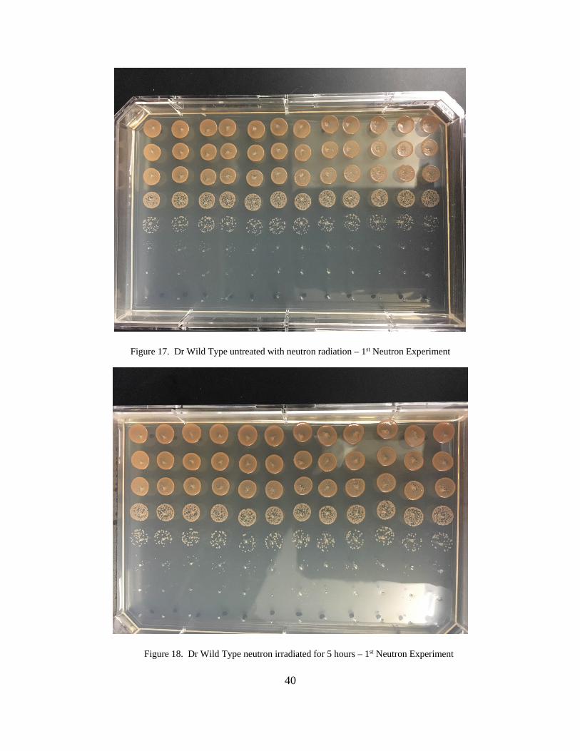
40
Figure 17. Dr Wild Type untreated with neutron radiation – 1st Neutron Experiment
Figure 18. Dr Wild Type neutron irradiated for 5 hours – 1st Neutron Experiment
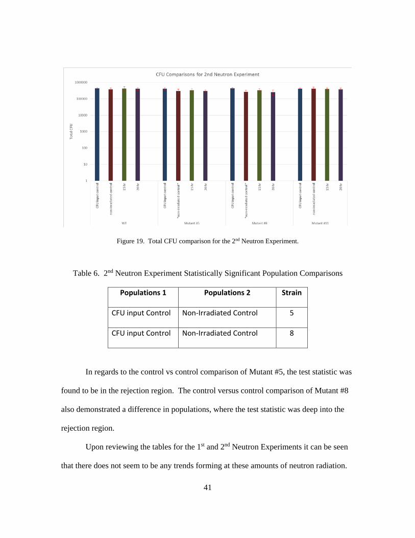
41
Figure 19. Total CFU comparison for the 2nd Neutron Experiment.
Table 6. 2nd Neutron Experiment Statistically Significant Population Comparisons
Populations 1 Populations 2 Strain
CFU input Control Non-Irradiated Control 5
CFU input Control Non-Irradiated Control 8
In regards to the control vs control comparison of Mutant #5, the test statistic was
found to be in the rejection region. The control versus control comparison of Mutant #8
also demonstrated a difference in populations, where the test statistic was deep into the
rejection region.
Upon reviewing the tables for the 1st and 2nd Neutron Experiments it can be seen
that there does not seem to be any trends forming at these amounts of neutron radiation.
42
Of all comparisons that showed a statistical difference or close to a statistical difference
populations for these first two experiments, the latter two did not involve radiation, only
dehydration.
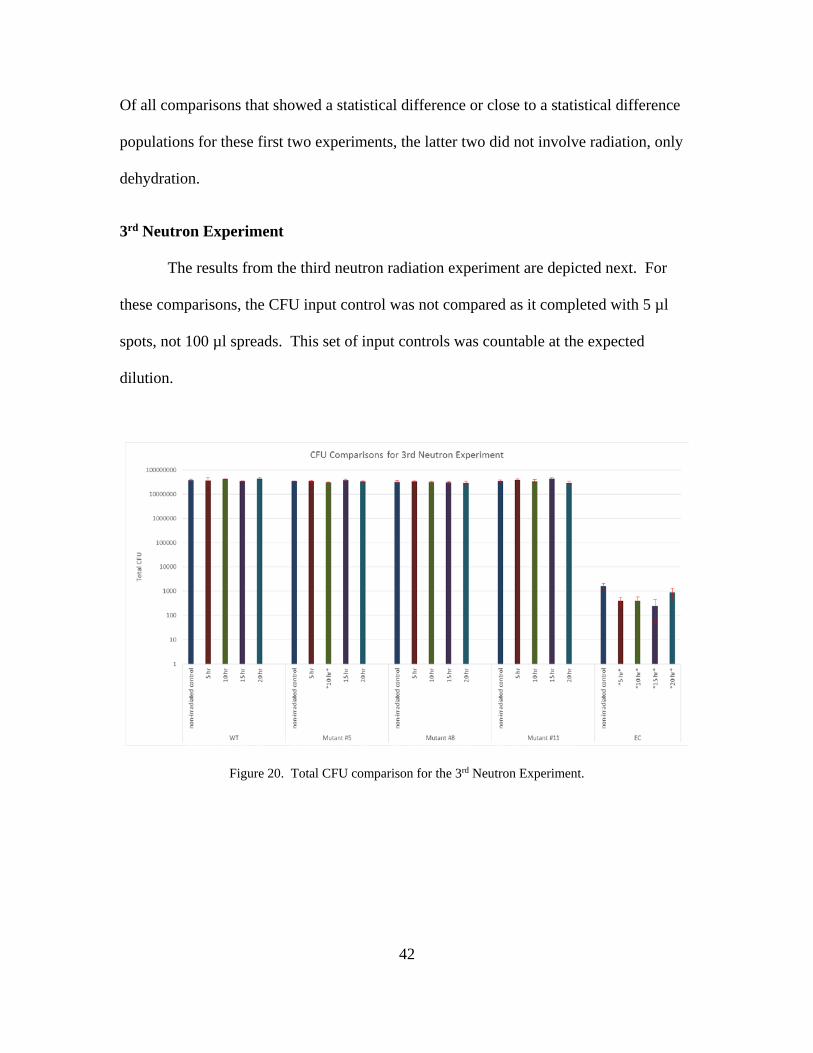
3rd Neutron Experiment
The results from the third neutron radiation experiment are depicted next. For
these comparisons, the CFU input control was not compared as it completed with 5 µl
spots, not 100 µl spreads. This set of input controls was countable at the expected
dilution.
Figure 20. Total CFU comparison for the 3rd Neutron Experiment.

43
Table 7. 3rd Neutron Experiment Statistically Significant Population Comparisons
Populations 1 Populations 2 Strain
Non-Irradiated Control 10 Hour Dose – 2.3 cGy 5
Non-Irradiated Control 5 Hour Dose – 1.1 cGy EC
Non-Irradiated Control 10 Hour Dose – 2.3 cGy EC
Non-Irradiated Control 15 Hour Dose – 3.4 cGy EC
Non-Irradiated Control 20 Hour Dose – 4.6 cGy EC
In regards to Mutant #5’s entry, the test statistic was deeply within the rejection
region. Like the previous experiments, no trends are readily apparent. This time, the
only the difference between populations occurred between the non-irradiated control and
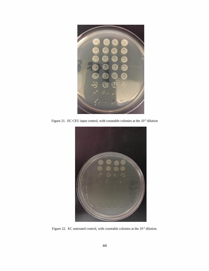
10 hour dose to Mutant #5’s samples. However, E. coli did show a sensitivity to both
desiccation and neutron treatment. EC’s CFU input controls showed countable colonies
starting at a 10-5 dilution, but the untreated control only had countable colonies at the 10-2
dilution. Additionally, the neutron radiation also had an effect on EC, unlike Dr.
44
Figure 21. EC CFU input control, with countable colonies at the 10-5 dilution
Figure 22. EC untreated control, with countable colonies at the 10-2 dilution.
45
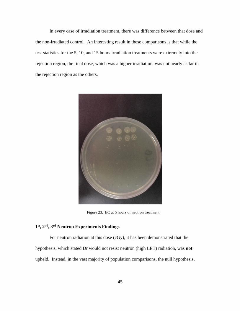
In every case of irradiation treatment, there was difference between that dose and
the non-irradiated control. An interesting result in these comparisons is that while the
test statistics for the 5, 10, and 15 hours irradiation treatments were extremely into the
rejection region, the final dose, which was a higher irradiation, was not nearly as far in
the rejection region as the others.
Figure 23. EC at 5 hours of neutron treatment.
1st, 2nd, 3rd Neutron Experiments Findings
For neutron radiation at this dose (cGy), it has been demonstrated that the
hypothesis, which stated Dr would not resist neutron (high LET) radiation, was not
upheld. Instead, in the vast majority of population comparisons, the null hypothesis,
46
which stated the populations of the experimental groups (neutron radiated) and control
groups (no radiation) would not be statistically different, could not be disproved.
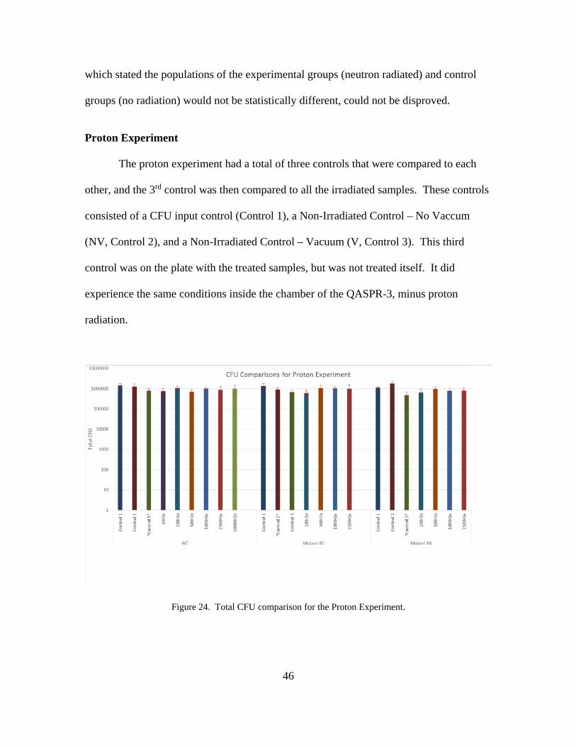
Proton Experiment
The proton experiment had a total of three controls that were compared to each
other, and the 3rd control was then compared to all the irradiated samples. These controls
consisted of a CFU input control (Control 1), a Non-Irradiated Control – No Vaccum
(NV, Control 2), and a Non-Irradiated Control – Vacuum (V, Control 3). This third
control was on the plate with the treated samples, but was not treated itself. It did
experience the same conditions inside the chamber of the QASPR-3, minus proton
radiation.
Figure 24. Total CFU comparison for the Proton Experiment.
47
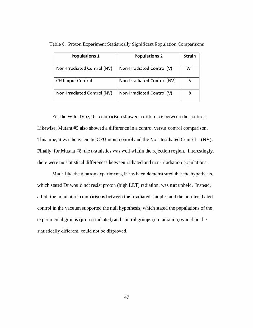
Table 8. Proton Experiment Statistically Significant Population Comparisons
Populations 1 Populations 2 Strain
Non-Irradiated Control (NV) Non-Irradiated Control (V) WT
CFU Input Control Non-Irradiated Control (NV) 5
Non-Irradiated Control (NV) Non-Irradiated Control (V) 8
For the Wild Type, the comparison showed a difference between the controls.
Likewise, Mutant #5 also showed a difference in a control versus control comparison.
This time, it was between the CFU input control and the Non-Irradiated Control – (NV).
Finally, for Mutant #8, the t-statistics was well within the rejection region. Interestingly,
there were no statistical differences between radiated and non-irradiation populations.
Much like the neutron experiments, it has been demonstrated that the hypothesis,
which stated Dr would not resist proton (high LET) radiation, was not upheld. Instead,
all of the population comparisons between the irradiated samples and the non-irradiated
control in the vacuum supported the null hypothesis, which stated the populations of the
experimental groups (proton radiated) and control groups (no radiation) would not be
statistically different, could not be disproved.
48
V. Conclusions and Recommendations
Conclusions of Research
These experiments have shown that not only is Dr resistant low LET radiation,
but high LET radiation as well. For the neutron experiments, the low amount of radiation
(no greater than cGy), seems to account for the lack of consistent effect of neutron
irradiation. It was already demonstrated that Dr can receive a dose of 5 kGy of ionizing
radiation of low LET with no lethality. [11] Likewise, previous experiments have shown
a gamma dose of 10 kGy will still result in survival close to only 10-2 lethality.[3] It is
reasonable to assume that the low amount of radiation is why the neutron irradiation
resulted in no lethality.
However, at the surface, the proton experiment seems to be at odds with the
findings of Paulino-Lima et al. In their study in regards to proton irradiation found in
solar winds, the researchers used lower energy protons (200 keV protons, not 4.5 MeV
protons) and had a greater LET (6.24 eV / Angstrom, compared to .86 eV / Angstrom).
Taking this a step further, researchers found that dried plasmids exposed to 10 MeV
protons, with 6.39 keV/µm LET resulted in 2.8 DSB/1000 Mbp-Gy.[22] The Mbp is the
number of mega base pairs per plasmid. If you combine Dr’s number of base pairs per
DNA (3.06 Mbp) and plasmids (233 Kbp)[5], you get a total of 3.293 Mbp. Since both
the energy and LET of the protons are on about the same order of magnitude (the LET for
the proton experiment was .85 eV/Angstrom = 8.5 keV/ µm, and the energy of the
protons was 4.5 MeV), an estimate of the number of DSB based on the number of Dr’s
49
Mbp and the irradiation dosage it received. This estimate is an upper level estimate, as
the plasmids presented no other biological targets, unlike the cells of Dr.
2.8 𝐷𝐷𝐷𝐷𝐷𝐷1000 𝑀𝑀𝑀𝑀𝐷𝐷 − 𝐺𝐺𝐺𝐺
∗ 3.293 𝑀𝑀𝑀𝑀𝐷𝐷 ∗ 10 𝐺𝐺𝐺𝐺 = .09 𝐷𝐷𝐷𝐷𝐷𝐷
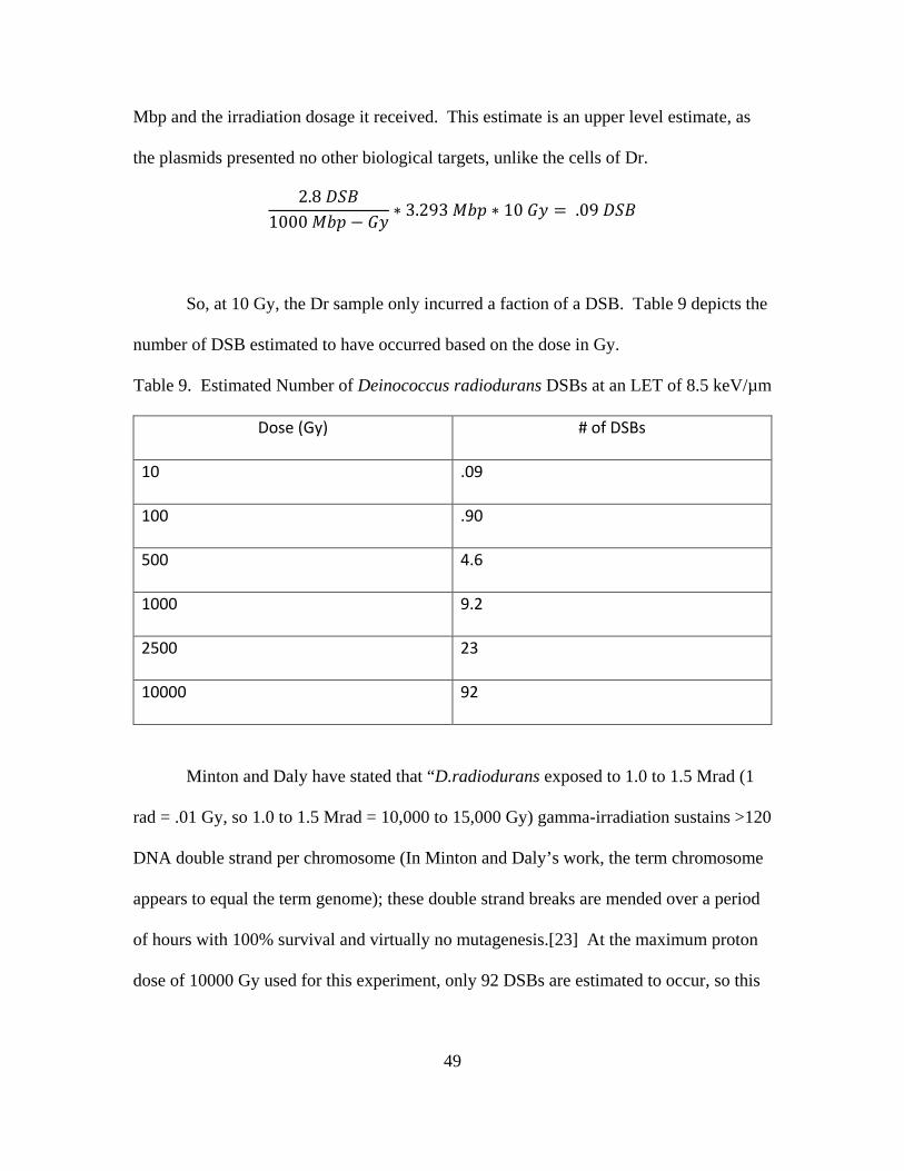
So, at 10 Gy, the Dr sample only incurred a faction of a DSB. Table 9 depicts the
number of DSB estimated to have occurred based on the dose in Gy.
Table 9. Estimated Number of Deinococcus radiodurans DSBs at an LET of 8.5 keV/µm
Dose (Gy) # of DSBs
10 .09
100 .90
500 4.6
1000 9.2
2500 23
10000 92
Minton and Daly have stated that “D.radiodurans exposed to 1.0 to 1.5 Mrad (1
rad = .01 Gy, so 1.0 to 1.5 Mrad = 10,000 to 15,000 Gy) gamma-irradiation sustains >120
DNA double strand per chromosome (In Minton and Daly’s work, the term chromosome
appears to equal the term genome); these double strand breaks are mended over a period
of hours with 100% survival and virtually no mutagenesis.[23] At the maximum proton
dose of 10000 Gy used for this experiment, only 92 DSBs are estimated to occur, so this
50
may be why there were no differences between the non-irradiated controls and the proton
irradiated samples.
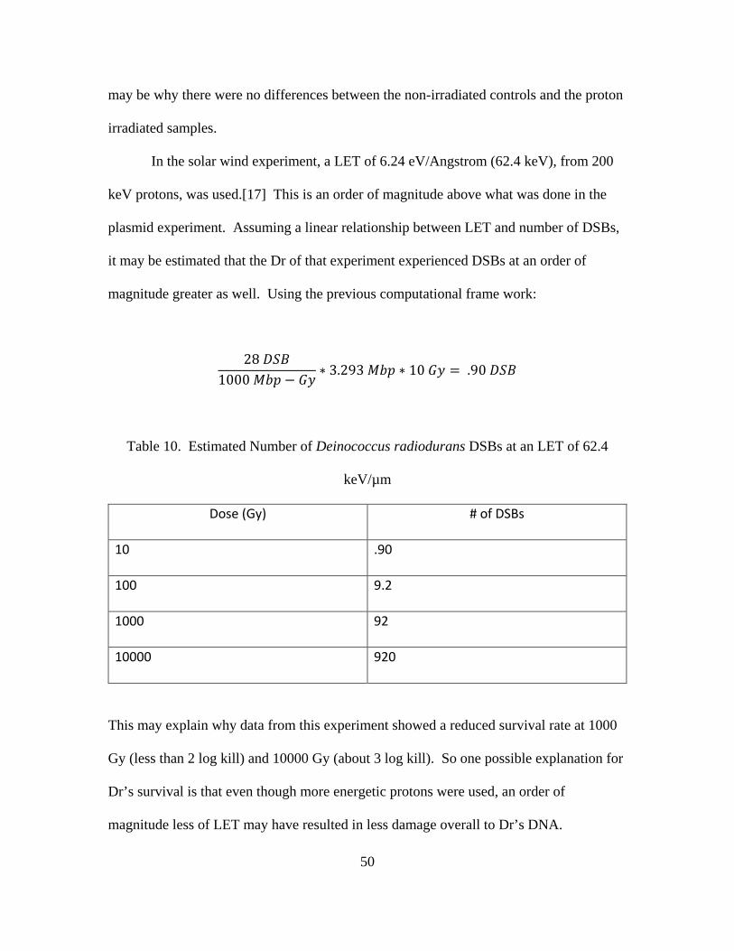
In the solar wind experiment, a LET of 6.24 eV/Angstrom (62.4 keV), from 200
keV protons, was used.[17] This is an order of magnitude above what was done in the
plasmid experiment. Assuming a linear relationship between LET and number of DSBs,
it may be estimated that the Dr of that experiment experienced DSBs at an order of
magnitude greater as well. Using the previous computational frame work:
28 𝐷𝐷𝐷𝐷𝐷𝐷1000 𝑀𝑀𝑀𝑀𝐷𝐷 − 𝐺𝐺𝐺𝐺
∗ 3.293 𝑀𝑀𝑀𝑀𝐷𝐷 ∗ 10 𝐺𝐺𝐺𝐺 = .90 𝐷𝐷𝐷𝐷𝐷𝐷
Table 10. Estimated Number of Deinococcus radiodurans DSBs at an LET of 62.4
keV/µm
Dose (Gy) # of DSBs
10 .90
100 9.2
1000 92
10000 920
This may explain why data from this experiment showed a reduced survival rate at 1000
Gy (less than 2 log kill) and 10000 Gy (about 3 log kill). So one possible explanation for
Dr’s survival is that even though more energetic protons were used, an order of
magnitude less of LET may have resulted in less damage overall to Dr’s DNA.
51
Interestingly, no single mutant stood out as being more sensitive to the proton
irradiation. The mutant gene KOs were devised to disrupt pathways which protected
against radicals resulting from indirect damage caused by low LET. This adds validity to
the idea that indirect damage is more detrimental to Dr’s ability to repair itself than direct
damage.[22] Because of the ability to survive around a hundred DSBs, the protective
mechanism at play seems to be Dr’s capability to repair DNA DSBs.
Another major difference between the experiments was in the method used to
create a sample. The researchers in Survival of Deinococcus radiodurans Against
Laboratory-Simulated Solar Wind Charged Particles used a monolayer of cells. This
was done to prevent irradiation shielding from dead cells. Because this experiment had
more layers, there may have been some shielding. Likewise, some shielding may have
occurred from the organic molecules of the TGY cell medium that did not evaporate
while Dr was left to dehydrate under the biosafety cabinet.
Finally, the mechanisms normally associated with desiccation may have already
been up-regulated during the de-hydration process. As such, this may have given Dr an
advantage in repair during rehydration and re-growth.
Recommendations for Future Research
The results of these experiments certainly lead to more questions for future
research. On such question is in regards to the neutron research. The neutron generator
available at the Air Force Institute of Technology was somewhat limited in that it could
only produce a 109 neutrons per second, without consideration of geometric attenuation.
If possible, subjecting Dr to greater neutron fluxes may result in greater lethality than
52
demonstrated in this experiment. Possible neutron sources include the Ohio State
University Research Reactor, which is capable of neutron fluxes in the order of
magnitude of 1013 n/cm2/s, though these neutrons are thermal neutrons, not fast neutrons
like those used in this experiment.[24] Another venue for greater neutron flux is the
Spallation Neutron Source located at Oak Ridge National Laboratory.
Another interesting aspect of this research would be looking at another type of
high LET radiation, such as alpha particles, which are essentially helium ions. The
QASAR-3 is also able to produce this type of ion as well. If feasible, changing the
sample preparation to a monolayer and washing of the cells to prevent shielding may also
yield different results then were shown in the proton experiment during this research.
Further researcher may also need to consider the LET, not the just the energy of the
particles used for irradiation.
53
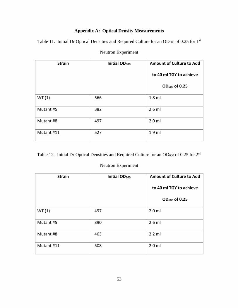
Appendix A: Optical Density Measurements
Table 11. Initial Dr Optical Densities and Required Culture for an OD600 of 0.25 for 1st
Neutron Experiment
Strain Initial OD600 Amount of Culture to Add
to 40 ml TGY to achieve
OD600 of 0.25
WT (1) .566 1.8 ml
Mutant #5 .382 2.6 ml
Mutant #8 .497 2.0 ml
Mutant #11 .527 1.9 ml
Table 12. Initial Dr Optical Densities and Required Culture for an OD600 of 0.25 for 2nd
Neutron Experiment
Strain Initial OD600 Amount of Culture to Add
to 40 ml TGY to achieve
OD600 of 0.25
WT (1) .497 2.0 ml
Mutant #5 .390 2.6 ml
Mutant #8 .463 2.2 ml
Mutant #11 .508 2.0 ml
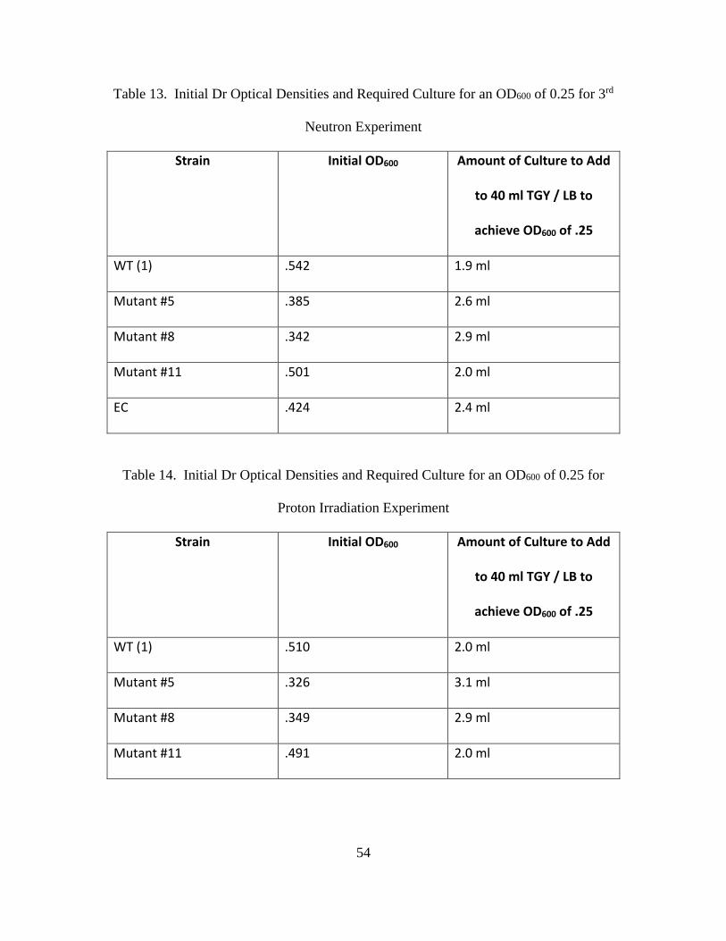
54
Table 13. Initial Dr Optical Densities and Required Culture for an OD600 of 0.25 for 3rd
Neutron Experiment
Strain Initial OD600 Amount of Culture to Add
to 40 ml TGY / LB to
achieve OD600 of .25
WT (1) .542 1.9 ml
Mutant #5 .385 2.6 ml
Mutant #8 .342 2.9 ml
Mutant #11 .501 2.0 ml
EC .424 2.4 ml
Table 14. Initial Dr Optical Densities and Required Culture for an OD600 of 0.25 for
Proton Irradiation Experiment
Strain Initial OD600 Amount of Culture to Add
to 40 ml TGY / LB to
achieve OD600 of .25
WT (1) .510 2.0 ml
Mutant #5 .326 3.1 ml
Mutant #8 .349 2.9 ml
Mutant #11 .491 2.0 ml
55
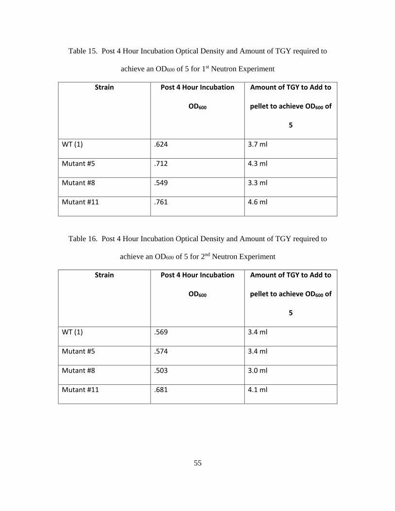
Table 15. Post 4 Hour Incubation Optical Density and Amount of TGY required to
achieve an OD600 of 5 for 1st Neutron Experiment
Strain Post 4 Hour Incubation
OD600
Amount of TGY to Add to
pellet to achieve OD600 of
5
WT (1) .624 3.7 ml
Mutant #5 .712 4.3 ml
Mutant #8 .549 3.3 ml
Mutant #11 .761 4.6 ml
Table 16. Post 4 Hour Incubation Optical Density and Amount of TGY required to
achieve an OD600 of 5 for 2nd Neutron Experiment
Strain Post 4 Hour Incubation
OD600
Amount of TGY to Add to
pellet to achieve OD600 of
5
WT (1) .569 3.4 ml
Mutant #5 .574 3.4 ml
Mutant #8 .503 3.0 ml
Mutant #11 .681 4.1 ml
56
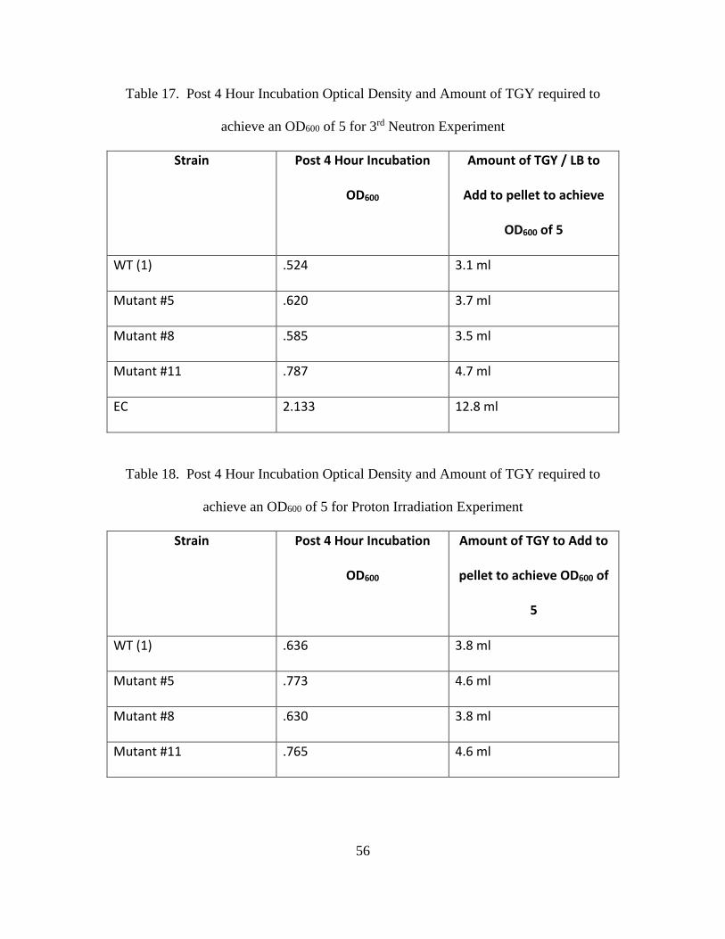
Table 17. Post 4 Hour Incubation Optical Density and Amount of TGY required to
achieve an OD600 of 5 for 3rd Neutron Experiment
Strain Post 4 Hour Incubation
OD600
Amount of TGY / LB to
Add to pellet to achieve
OD600 of 5
WT (1) .524 3.1 ml
Mutant #5 .620 3.7 ml
Mutant #8 .585 3.5 ml
Mutant #11 .787 4.7 ml
EC 2.133 12.8 ml
Table 18. Post 4 Hour Incubation Optical Density and Amount of TGY required to
achieve an OD600 of 5 for Proton Irradiation Experiment
Strain Post 4 Hour Incubation
OD600
Amount of TGY to Add to
pellet to achieve OD600 of
5
WT (1) .636 3.8 ml
Mutant #5 .773 4.6 ml
Mutant #8 .630 3.8 ml
Mutant #11 .765 4.6 ml
57
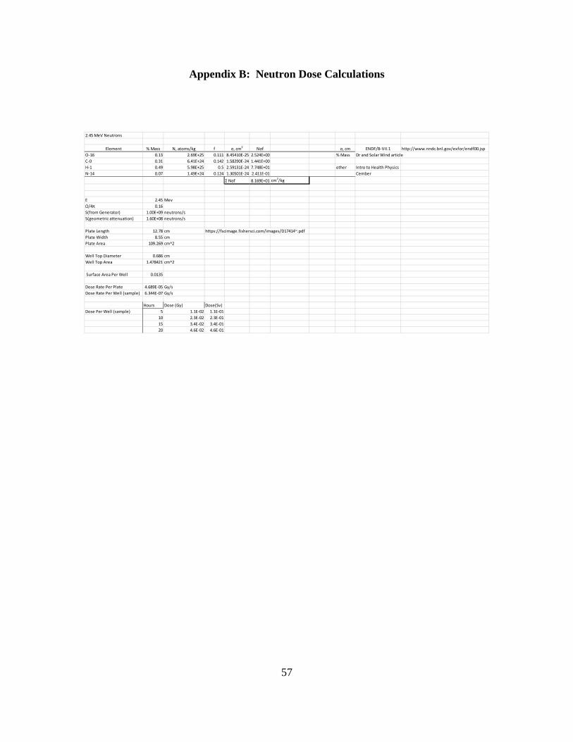
Appendix B: Neutron Dose Calculations
2.45 MeV Neutrons
Element % Mass N, atoms/kg f σ, cm2 Nσf σ, cm ENDF/B-VII.1 http://www.nndc.bnl.gov/exfor/endf00.jspO-16 0.13 2.69E+25 0.111 8.45410E-25 2.524E+00 % Mass Dr and Solar Wind articleC-0 0.31 6.41E+24 0.142 1.58290E-24 1.441E+00H-1 0.49 5.98E+25 0.5 2.59131E-24 7.748E+01 other Intro to Health PhysicsN-14 0.07 1.49E+24 0.124 1.30501E-24 2.411E-01 Cember
Σ Nσf 8.169E+01 cm2/kg
E 2.45 MevΩ/4π 0.16S(from Generator) 1.00E+09 neutrons/sS(geometric attenuation) 1.60E+08 neutrons/s
Plate Length 12.78 cm https://fscimage.fishersci.com/images/D17414~.pdfPlate Width 8.55 cmPlate Area 109.269 cm^2
Well Top Diameter 0.686 cmWell Top Area 1.478421 cm^2
Surface Area Per Well 0.0135
Dose Rate Per Plate 4.689E-05 Gy/sDose Rate Per Well (sample) 6.344E-07 Gy/s
Hours Dose (Gy) Dose(Sv)Dose Per Well (sample) 5 1.1E-02 1.1E-01
10 2.3E-02 2.3E-0115 3.4E-02 3.4E-0120 4.6E-02 4.6E-01
58
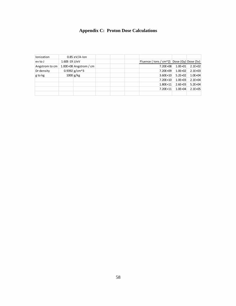
Appendix C: Proton Dose Calculations
Ionization 0.85 eV/A-Ionev to J 1.60E-19 J/eV Fluence ( Ions / cm^2) Dose (Gy) Dose (Sv)Angstrom to cm 1.00E+08 Angstrom / cm 7.20E+08 1.0E+01 2.1E+02Dr density 0.9392 g/cm^3 7.20E+09 1.0E+02 2.1E+03g to kg 1000 g/kg 3.60E+10 5.2E+02 1.0E+04
7.20E+10 1.0E+03 2.1E+041.80E+11 2.6E+03 5.2E+047.20E+11 1.0E+04 2.1E+05
59
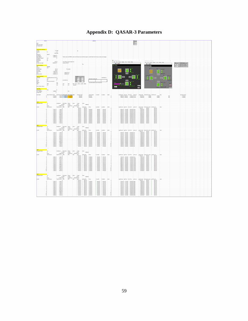
Appendix D: QASAR-3 Parameters
170117 1.00E+09
AFITMaj. Ron LenkerDr. Adam Cahil
Accelerator conditionsEnergy 4.5 MeV apSpecies H 1+tv 1.435 MeVBeamline qaspr3Ext Magnet -1.00E+03 GMain Magnet 6.24E-02 G Tried to steer with MM in order to shift beam over with Ext magnet, since BL Obj slit all the way out does not engage.45 degree magnet n/a GLE Blanker onHE Blanker onBHE bl 4.25 µs set to 30 usec pulse alignmentfaraday cup suppr 2.606E+02 V checked 161122
Apbeam conditionstest DRBugs!camera DS-1camera mag 9.6 err 0.1 µm/pxovl pulse 100 µsarea pulse 7.73E-02 µsarea 7.73E-02 err 5.93E-04 cm2beam current 4.50E+01 err 3.00E+00 nA
device conditionsDRbugA5 multiple positions on row 1 marking locnIe n/a uA Die matrix location #stemp RT K no control on 3 2 1posn first one on the left 6 5 4M2 thk µm very thin bottom strip not exposedVBB VRB VEE VCC VRC VBC = (VCC - |VRC|) – (VBB - |VRB|)
n/a n/a n/a n/a #VALUE!Set A, Plate 5, Row 1
test shotsDrbug-test2 test #TIA - K428 gain 1.00E+06 V/Acharge state 2
test shot# device fluence /cm2 avg fluence targepulse (nom) pulse target (sec) TIA gain (V/A) pulse (meas) k_fact(1) k_fact(n) index avg fluence avg fl err dev fl err pulse err pulse (calc) fluence/us error calc fl/us err freq dev/avg fl ratio0 5.55E+08 7.20E+09 1.000E-04 1.957E-03 1.00E+08 99.1473u 0 3.68E+08 5.84E+06 4.11E+07 247.1n 9.9147E-05 0.000% 0.000% 100 1.51E+001 1.10E+10 7.29E+09 1.000E-04 1.000E-04 1.00E+08 1.96146m 0 7.29E+09 2.43E+08 8.76E+08 11.45u 1.9615E-03 0.000% 0.000% 100 1.51E+00
SHOTDRbugA5-R1W1 _# irradiation 4x3 matrix Xstep 2mm ystep 3mm
H 4.5 MeV charge 1 gain 1.00E+06Pulse 1.960E-03 sec target fluenc 7.29E+09 /cm2
shot # Shot Fluence Total Fluence VRB VRC VRE Gain delta(1/G) Pulse k_fact(1) k_fact(n) index avg fluence avg fl err dev fl err pulse err pulse (calc) fluence/us error calc fl/us err note- 0 #DIV/0! #DIV/0! 0 #VALUE! #DIV/0! #DIV/0!
0 1.18E+10 1.18E+10 #DIV/0! #DIV/0! 2.00134m #DIV/0! #VALUE! 1 7.82E+09 1.61E+08 8.87E+08 16.4u 2.0013E-03 #DIV/0! #DIV/0!1 1.18E+10 2.36E+10 #DIV/0! #DIV/0! 2.00134m #DIV/0! #VALUE! 2 7.82E+09 1.61E+08 8.87E+08 16.4u 2.0013E-03 #DIV/0! #DIV/0!2 1.18E+10 3.54E+10 #DIV/0! #DIV/0! 2.00134m #DIV/0! #VALUE! 3 7.82E+09 1.61E+08 8.87E+08 16.4u 2.0013E-03 #DIV/0! #DIV/0!3 1.18E+10 4.72E+10 #DIV/0! #DIV/0! 2.00134m #DIV/0! #VALUE! 4 7.82E+09 1.61E+08 8.87E+08 16.4u 2.0013E-03 #DIV/0! #DIV/0!4 1.18E+10 5.90E+10 #DIV/0! #DIV/0! 2.00134m #DIV/0! #VALUE! 5 7.82E+09 1.61E+08 8.87E+08 16.4u 2.0013E-03 #DIV/0! #DIV/0!5 1.18E+10 7.07E+10 #DIV/0! #DIV/0! 2.00134m #DIV/0! #VALUE! 6 7.82E+09 1.61E+08 8.87E+08 16.4u 2.0013E-03 #DIV/0! #DIV/0!6 1.18E+10 8.25E+10 #DIV/0! #DIV/0! 2.00134m #DIV/0! #VALUE! 7 7.82E+09 1.61E+08 8.87E+08 16.4u 2.0013E-03 #DIV/0! #DIV/0!7 1.18E+10 9.43E+10 #DIV/0! #DIV/0! 2.00134m #DIV/0! #VALUE! 8 7.82E+09 1.61E+08 8.87E+08 16.4u 2.0013E-03 #DIV/0! #DIV/0!8 1.18E+10 1.06E+11 #DIV/0! #DIV/0! 2.00134m #DIV/0! #VALUE! 9 7.82E+09 1.61E+08 8.87E+08 16.4u 2.0013E-03 #DIV/0! #DIV/0!9 1.18E+10 1.18E+11 #DIV/0! #DIV/0! 2.00134m #DIV/0! #VALUE! 10 7.82E+09 1.61E+08 8.87E+08 16.4u 2.0013E-03 #DIV/0! #DIV/0!
10 1.18E+10 1.30E+11 #DIV/0! #DIV/0! 2.00134m #DIV/0! #VALUE! 11 7.82E+09 1.61E+08 8.87E+08 16.4u 2.0013E-03 #DIV/0! #DIV/0!11 1.18E+10 1.41E+11 #DIV/0! #DIV/0! 2.00134m #DIV/0! #VALUE! 12 7.82E+09 1.61E+08 8.87E+08 16.4u 2.0013E-03 #DIV/0! #DIV/0!
SHOTDRbugA5-R1W2 _# irradiation 4x3 matrix Xstep 2mm ystep 3mm
H 4.5 MeV charge 1 gain 1.00E+06Pulse 1.960E-03 sec target fluenc 7.29E+09 /cm2
shot # Shot Fluence Total Fluence VRB VRC VRE Gain delta(1/G) Pulse k_fact(1) k_fact(n) index avg fluence avg fl err dev fl err pulse err pulse (calc) fluence/us error calc fl/us err note- 0 #DIV/0! #DIV/0! 0 #VALUE! #DIV/0! #DIV/0!
0 1.10E+10 1.10E+10 #DIV/0! #DIV/0! 1.96176m #DIV/0! #VALUE! 1 7.32E+09 2.40E+08 8.76E+08 13u 1.9618E-03 #DIV/0! #DIV/0!1 1.10E+10 2.21E+10 #DIV/0! #DIV/0! 1.96176m #DIV/0! #VALUE! 2 7.32E+09 2.40E+08 8.76E+08 13u 1.9618E-03 #DIV/0! #DIV/0!2 1.10E+10 3.31E+10 #DIV/0! #DIV/0! 1.96176m #DIV/0! #VALUE! 3 7.32E+09 2.40E+08 8.76E+08 13u 1.9618E-03 #DIV/0! #DIV/0!3 1.10E+10 4.41E+10 #DIV/0! #DIV/0! 1.96176m #DIV/0! #VALUE! 4 7.32E+09 2.40E+08 8.76E+08 13u 1.9618E-03 #DIV/0! #DIV/0!4 1.10E+10 5.52E+10 #DIV/0! #DIV/0! 1.96176m #DIV/0! #VALUE! 5 7.32E+09 2.40E+08 8.76E+08 13u 1.9618E-03 #DIV/0! #DIV/0!5 1.10E+10 6.62E+10 #DIV/0! #DIV/0! 1.96176m #DIV/0! #VALUE! 6 7.32E+09 2.40E+08 8.76E+08 13u 1.9618E-03 #DIV/0! #DIV/0!6 1.10E+10 7.72E+10 #DIV/0! #DIV/0! 1.96176m #DIV/0! #VALUE! 7 7.32E+09 2.40E+08 8.76E+08 13u 1.9618E-03 #DIV/0! #DIV/0!7 1.10E+10 8.82E+10 #DIV/0! #DIV/0! 1.96176m #DIV/0! #VALUE! 8 7.32E+09 2.40E+08 8.76E+08 13u 1.9618E-03 #DIV/0! #DIV/0!8 1.10E+10 9.93E+10 #DIV/0! #DIV/0! 1.96176m #DIV/0! #VALUE! 9 7.32E+09 2.40E+08 8.76E+08 13u 1.9618E-03 #DIV/0! #DIV/0!9 1.10E+10 1.10E+11 #DIV/0! #DIV/0! 1.96176m #DIV/0! #VALUE! 10 7.32E+09 2.40E+08 8.76E+08 13u 1.9618E-03 #DIV/0! #DIV/0!
10 1.10E+10 1.21E+11 #DIV/0! #DIV/0! 1.96176m #DIV/0! #VALUE! 11 7.32E+09 2.40E+08 8.76E+08 13u 1.9618E-03 #DIV/0! #DIV/0!11 1.10E+10 1.32E+11 #DIV/0! #DIV/0! 1.96176m #DIV/0! #VALUE! 12 7.32E+09 2.40E+08 8.76E+08 13u 1.9618E-03 #DIV/0! #DIV/0!
SHOTDRbugA5-R1W3 _# irradiation 4x3 matrix Xstep 2mm ystep 3mm
H 4.5 MeV charge 1 gain 1.00E+06Pulse 1.960E-03 sec target fluenc 7.29E+09 /cm2
shot # Shot Fluence Total Fluence VRB VRC VRE Gain delta(1/G) Pulse k_fact(1) k_fact(n) index avg fluence avg fl err dev fl err pulse err pulse (calc) fluence/us error calc fl/us err note- 0 #DIV/0! #DIV/0! 0 #VALUE! #DIV/0! #DIV/0!
0 1.08E+10 1.08E+10 #DIV/0! #DIV/0! 1.95506m #DIV/0! #VALUE! 1 7.16E+09 2.02E+08 8.39E+08 10.2u 1.9551E-03 #DIV/0! #DIV/0!1 7.29E+10 8.37E+10 #DIV/0! #DIV/0! 1.07633m #DIV/0! #VALUE! 2 4.48E+10 7.66E+08 2.43E+09 1.053u 1.0763E-03 #DIV/0! #DIV/0!2 7.29E+10 1.57E+11 #DIV/0! #DIV/0! 1.07633m #DIV/0! #VALUE! 3 4.48E+10 7.66E+08 2.43E+09 1.053u 1.0763E-03 #DIV/0! #DIV/0!3 7.29E+10 2.30E+11 #DIV/0! #DIV/0! 1.07633m #DIV/0! #VALUE! 4 4.48E+10 7.66E+08 2.43E+09 1.053u 1.0763E-03 #DIV/0! #DIV/0!4 7.29E+10 3.03E+11 #DIV/0! #DIV/0! 1.07633m #DIV/0! #VALUE! 5 4.48E+10 7.66E+08 2.43E+09 1.053u 1.0763E-03 #DIV/0! #DIV/0!5 7.29E+10 3.76E+11 #DIV/0! #DIV/0! 1.07633m #DIV/0! #VALUE! 6 4.48E+10 7.66E+08 2.43E+09 1.053u 1.0763E-03 #DIV/0! #DIV/0!6 7.29E+10 4.48E+11 #DIV/0! #DIV/0! 1.07633m #DIV/0! #VALUE! 7 4.48E+10 7.66E+08 2.43E+09 1.053u 1.0763E-03 #DIV/0! #DIV/0!7 7.29E+10 5.21E+11 #DIV/0! #DIV/0! 1.07633m #DIV/0! #VALUE! 8 4.48E+10 7.66E+08 2.43E+09 1.053u 1.0763E-03 #DIV/0! #DIV/0!8 7.29E+10 5.94E+11 #DIV/0! #DIV/0! 1.07633m #DIV/0! #VALUE! 9 4.48E+10 7.66E+08 2.43E+09 1.053u 1.0763E-03 #DIV/0! #DIV/0!9 7.29E+10 6.67E+11 #DIV/0! #DIV/0! 1.07633m #DIV/0! #VALUE! 10 4.48E+10 7.66E+08 2.43E+09 1.053u 1.0763E-03 #DIV/0! #DIV/0!
10 7.29E+10 7.40E+11 #DIV/0! #DIV/0! 1.07633m #DIV/0! #VALUE! 11 4.48E+10 7.66E+08 2.43E+09 1.053u 1.0763E-03 #DIV/0! #DIV/0!11 7.29E+10 8.13E+11 #DIV/0! #DIV/0! 1.07633m #DIV/0! #VALUE! 12 4.48E+10 7.66E+08 2.43E+09 1.053u 1.0763E-03 #DIV/0! #DIV/0!
SHOTDRbugA5-R1W4 _# irradiation 4x3 matrix Xstep 2mm ystep 3mm
H 4.5 MeV charge 1 gain 1.00E+06Pulse 1.960E-03 sec target fluenc 7.29E+09 /cm2
shot # Shot Fluence Total Fluence VRB VRC VRE Gain delta(1/G) Pulse k_fact(1) k_fact(n) index avg fluence avg fl err dev fl err pulse err pulse (calc) fluence/us error calc fl/us err note- 0 #DIV/0! #DIV/0! 0 #VALUE! #DIV/0! #DIV/0!
0 1.09E+10 1.09E+10 #DIV/0! #DIV/0! 1.95535m #DIV/0! #VALUE! 1 7.25E+09 2.17E+08 8.56E+08 9.84u 1.9554E-03 #DIV/0! #DIV/0!1 1.09E+10 2.19E+10 #DIV/0! #DIV/0! 1.95535m #DIV/0! #VALUE! 2 7.25E+09 2.17E+08 8.56E+08 9.84u 1.9554E-03 #DIV/0! #DIV/0!2 1.09E+10 3.28E+10 #DIV/0! #DIV/0! 1.95535m #DIV/0! #VALUE! 3 7.25E+09 2.17E+08 8.56E+08 9.84u 1.9554E-03 #DIV/0! #DIV/0!3 1.09E+10 4.37E+10 #DIV/0! #DIV/0! 1.95535m #DIV/0! #VALUE! 4 7.25E+09 2.17E+08 8.56E+08 9.84u 1.9554E-03 #DIV/0! #DIV/0!4 1.09E+10 5.47E+10 #DIV/0! #DIV/0! 1.95535m #DIV/0! #VALUE! 5 7.25E+09 2.17E+08 8.56E+08 9.84u 1.9554E-03 #DIV/0! #DIV/0!5 1.09E+10 6.56E+10 #DIV/0! #DIV/0! 1.95535m #DIV/0! #VALUE! 6 7.25E+09 2.17E+08 8.56E+08 9.84u 1.9554E-03 #DIV/0! #DIV/0!6 1.09E+10 7.65E+10 #DIV/0! #DIV/0! 1.95535m #DIV/0! #VALUE! 7 7.25E+09 2.17E+08 8.56E+08 9.84u 1.9554E-03 #DIV/0! #DIV/0!7 1.09E+10 8.74E+10 #DIV/0! #DIV/0! 1.95535m #DIV/0! #VALUE! 8 7.25E+09 2.17E+08 8.56E+08 9.84u 1.9554E-03 #DIV/0! #DIV/0!8 1.09E+10 9.84E+10 #DIV/0! #DIV/0! 1.95535m #DIV/0! #VALUE! 9 7.25E+09 2.17E+08 8.56E+08 9.84u 1.9554E-03 #DIV/0! #DIV/0!9 1.09E+10 1.09E+11 #DIV/0! #DIV/0! 1.95535m #DIV/0! #VALUE! 10 7.25E+09 2.17E+08 8.56E+08 9.84u 1.9554E-03 #DIV/0! #DIV/0!
10 1.09E+10 1.20E+11 #DIV/0! #DIV/0! 1.95535m #DIV/0! #VALUE! 11 7.25E+09 2.17E+08 8.56E+08 9.84u 1.9554E-03 #DIV/0! #DIV/0!11 1.09E+10 1.31E+11 #DIV/0! #DIV/0! 1.95535m #DIV/0! #VALUE! 12 7.25E+09 2.17E+08 8.56E+08 9.84u 1.9554E-03 #DIV/0! #DIV/0!
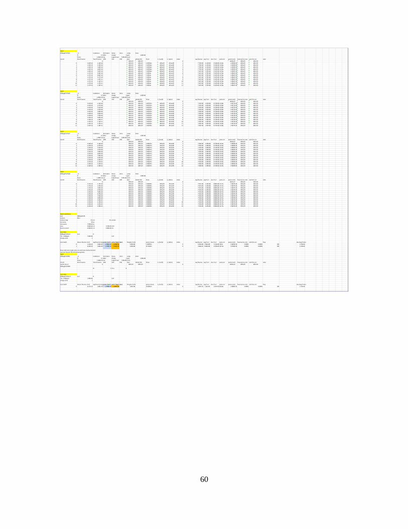
60
SHOTDRbugA5-R1W5 _# irradiation 4x3 matrix Xstep 2mm ystep 3mm
H 4.5 MeV charge 1 gain 1.00E+06Pulse 1.960E-03 sec target fluenc 7.29E+09 /cm2
shot # Shot Fluence Total Fluence VRB VRC VRE Gain delta(1/G) Pulse k_fact(1) k_fact(n) index avg fluence avg fl err dev fl err pulse err pulse (calc) fluence/us error calc fl/us err note- 0 #DIV/0! #DIV/0! 0 #VALUE! #DIV/0! #DIV/0!
0 1.16E+10 1.16E+10 #DIV/0! #DIV/0! 1.96354m #DIV/0! #VALUE! 1 7.72E+09 2.13E+08 9.01E+08 13.28u 1.9635E-03 #DIV/0! #DIV/0!1 1.16E+10 2.33E+10 #DIV/0! #DIV/0! 1.96354m #DIV/0! #VALUE! 2 7.72E+09 2.13E+08 9.01E+08 13.28u 1.9635E-03 #DIV/0! #DIV/0!2 1.16E+10 3.49E+10 #DIV/0! #DIV/0! 1.96354m #DIV/0! #VALUE! 3 7.72E+09 2.13E+08 9.01E+08 13.28u 1.9635E-03 #DIV/0! #DIV/0!3 1.16E+10 4.66E+10 #DIV/0! #DIV/0! 1.96354m #DIV/0! #VALUE! 4 7.72E+09 2.13E+08 9.01E+08 13.28u 1.9635E-03 #DIV/0! #DIV/0!4 1.16E+10 5.82E+10 #DIV/0! #DIV/0! 1.96354m #DIV/0! #VALUE! 5 7.41E+09 2.76E+08 9.10E+08 13.28u 1.9635E-03 #DIV/0! #DIV/0!5 1.12E+10 6.94E+10 #DIV/0! #DIV/0! 1.9601m #DIV/0! #VALUE! 6 7.41E+09 2.76E+08 9.10E+08 13.28u 1.9601E-03 #DIV/0! #DIV/0!6 1.12E+10 8.06E+10 #DIV/0! #DIV/0! 1.9601m #DIV/0! #VALUE! 7 7.41E+09 2.76E+08 9.10E+08 13.28u 1.9601E-03 #DIV/0! #DIV/0!7 1.12E+10 9.17E+10 #DIV/0! #DIV/0! 1.9601m #DIV/0! #VALUE! 8 7.41E+09 2.76E+08 9.10E+08 13.28u 1.9601E-03 #DIV/0! #DIV/0!8 1.12E+10 1.03E+11 #DIV/0! #DIV/0! 1.9601m #DIV/0! #VALUE! 9 7.41E+09 2.76E+08 9.10E+08 13.28u 1.9601E-03 #DIV/0! #DIV/0!9 1.12E+10 1.14E+11 #DIV/0! #DIV/0! 1.9601m #DIV/0! #VALUE! 10 7.41E+09 2.76E+08 9.10E+08 13.28u 1.9601E-03 #DIV/0! #DIV/0!
10 1.12E+10 1.25E+11 #DIV/0! #DIV/0! 1.9601m #DIV/0! #VALUE! 11 7.41E+09 2.76E+08 9.10E+08 13.28u 1.9601E-03 #DIV/0! #DIV/0!11 1.12E+10 1.36E+11 #DIV/0! #DIV/0! 1.9601m #DIV/0! #VALUE! 12 7.41E+09 2.76E+08 9.10E+08 13.28u 1.9601E-03 #DIV/0! #DIV/0!
SHOTDRbugA5-R1W6 _# irradiation 4x3 matrix Xstep 2mm ystep 3mm
H 4.5 MeV charge 1 gain 1.00E+06Pulse 1.960E-03 sec target fluenc 7.29E+09 /cm2
shot # Shot Fluence Total Fluence VRB VRC VRE Gain delta(1/G) Pulse k_fact(1) k_fact(n) index avg fluence avg fl err dev fl err pulse err pulse (calc) fluence/us error calc fl/us err note- 0 #DIV/0! #DIV/0! 0 #VALUE! #DIV/0! #DIV/0!
0 1.14E+10 1.14E+10 #DIV/0! #DIV/0! 1.96765m #DIV/0! #VALUE! 1 7.54E+09 1.95E+08 8.73E+08 15.08u 1.9677E-03 #DIV/0! #DIV/0!1 1.14E+10 2.27E+10 #DIV/0! #DIV/0! 1.96765m #DIV/0! #VALUE! 2 7.54E+09 1.95E+08 8.73E+08 15.08u 1.9677E-03 #DIV/0! #DIV/0!2 1.14E+10 3.41E+10 #DIV/0! #DIV/0! 1.96765m #DIV/0! #VALUE! 3 7.54E+09 1.95E+08 8.73E+08 15.08u 1.9677E-03 #DIV/0! #DIV/0!3 1.14E+10 4.54E+10 #DIV/0! #DIV/0! 1.96765m #DIV/0! #VALUE! 4 7.54E+09 1.95E+08 8.73E+08 15.08u 1.9677E-03 #DIV/0! #DIV/0!4 1.14E+10 5.68E+10 #DIV/0! #DIV/0! 1.96765m #DIV/0! #VALUE! 5 7.54E+09 1.95E+08 8.73E+08 15.08u 1.9677E-03 #DIV/0! #DIV/0!5 1.14E+10 6.82E+10 #DIV/0! #DIV/0! 1.96765m #DIV/0! #VALUE! 6 7.54E+09 1.95E+08 8.73E+08 15.08u 1.9677E-03 #DIV/0! #DIV/0!6 1.14E+10 7.95E+10 #DIV/0! #DIV/0! 1.96765m #DIV/0! #VALUE! 7 7.54E+09 1.95E+08 8.73E+08 15.08u 1.9677E-03 #DIV/0! #DIV/0!7 1.14E+10 9.09E+10 #DIV/0! #DIV/0! 1.96765m #DIV/0! #VALUE! 8 7.54E+09 1.95E+08 8.73E+08 15.08u 1.9677E-03 #DIV/0! #DIV/0!8 1.14E+10 1.02E+11 #DIV/0! #DIV/0! 1.96765m #DIV/0! #VALUE! 9 7.54E+09 1.95E+08 8.73E+08 15.08u 1.9677E-03 #DIV/0! #DIV/0!9 1.14E+10 1.14E+11 #DIV/0! #DIV/0! 1.96765m #DIV/0! #VALUE! 10 7.54E+09 1.95E+08 8.73E+08 15.08u 1.9677E-03 #DIV/0! #DIV/0!
10 1.14E+10 1.25E+11 #DIV/0! #DIV/0! 1.96765m #DIV/0! #VALUE! 11 7.54E+09 1.95E+08 8.73E+08 15.08u 1.9677E-03 #DIV/0! #DIV/0!11 1.14E+10 1.36E+11 #DIV/0! #DIV/0! 1.96765m #DIV/0! #VALUE! 12 7.54E+09 1.95E+08 8.73E+08 15.08u 1.9677E-03 #DIV/0! #DIV/0!
SHOTDRbugA5-R1W7 _# irradiation 4x3 matrix Xstep 2mm ystep 3mm
H 4.5 MeV charge 1 gain 1.00E+06Pulse 1.960E-03 sec target fluenc 7.29E+09 /cm2
shot # Shot Fluence Total Fluence VRB VRC VRE Gain delta(1/G) Pulse k_fact(1) k_fact(n) index avg fluence avg fl err dev fl err pulse err pulse (calc) fluence/us error calc fl/us err note- 0 #DIV/0! #DIV/0! 0 #VALUE! #DIV/0! #DIV/0!
0 1.14E+10 1.14E+10 #DIV/0! #DIV/0! 1.96627m #DIV/0! #VALUE! 1 7.54E+09 1.93E+08 8.73E+08 14.03u 1.9663E-03 #DIV/0! #DIV/0!1 1.14E+10 2.27E+10 #DIV/0! #DIV/0! 1.96627m #DIV/0! #VALUE! 2 7.54E+09 1.93E+08 8.73E+08 14.03u 1.9663E-03 #DIV/0! #DIV/0!2 1.14E+10 3.41E+10 #DIV/0! #DIV/0! 1.96627m #DIV/0! #VALUE! 3 7.54E+09 1.93E+08 8.73E+08 14.03u 1.9663E-03 #DIV/0! #DIV/0!3 1.14E+10 4.55E+10 #DIV/0! #DIV/0! 1.96627m #DIV/0! #VALUE! 4 7.54E+09 1.93E+08 8.73E+08 14.03u 1.9663E-03 #DIV/0! #DIV/0!4 1.14E+10 5.69E+10 #DIV/0! #DIV/0! 1.96627m #DIV/0! #VALUE! 5 7.54E+09 1.93E+08 8.73E+08 14.03u 1.9663E-03 #DIV/0! #DIV/0!5 1.14E+10 6.82E+10 #DIV/0! #DIV/0! 1.96627m #DIV/0! #VALUE! 6 7.54E+09 1.93E+08 8.73E+08 14.03u 1.9663E-03 #DIV/0! #DIV/0!6 1.14E+10 7.96E+10 #DIV/0! #DIV/0! 1.96627m #DIV/0! #VALUE! 7 7.54E+09 1.93E+08 8.73E+08 14.03u 1.9663E-03 #DIV/0! #DIV/0!7 1.14E+10 9.10E+10 #DIV/0! #DIV/0! 1.96627m #DIV/0! #VALUE! 8 7.54E+09 1.93E+08 8.73E+08 14.03u 1.9663E-03 #DIV/0! #DIV/0!8 1.14E+10 1.02E+11 #DIV/0! #DIV/0! 1.96627m #DIV/0! #VALUE! 9 7.54E+09 1.93E+08 8.73E+08 14.03u 1.9663E-03 #DIV/0! #DIV/0!9 1.14E+10 1.14E+11 #DIV/0! #DIV/0! 1.96627m #DIV/0! #VALUE! 10 7.54E+09 1.93E+08 8.73E+08 14.03u 1.9663E-03 #DIV/0! #DIV/0!
10 1.14E+10 1.25E+11 #DIV/0! #DIV/0! 1.96627m #DIV/0! #VALUE! 11 7.54E+09 1.93E+08 8.73E+08 14.03u 1.9663E-03 #DIV/0! #DIV/0!11 1.14E+10 1.36E+11 #DIV/0! #DIV/0! 1.96627m #DIV/0! #VALUE! 12 7.54E+09 1.93E+08 8.73E+08 14.03u 1.9663E-03 #DIV/0! #DIV/0!
SHOTDRbugA5-R1W8 _# irradiation 4x3 matrix Xstep 2mm ystep 3mm
H 4.5 MeV charge 1 gain 1.00E+06Pulse 1.960E-03 sec target fluenc 7.29E+09 /cm2
shot # Shot Fluence Total Fluence VRB VRC VRE Gain delta(1/G) Pulse k_fact(1) k_fact(n) index avg fluence avg fl err dev fl err pulse err pulse (calc) fluence/us error calc fl/us err note- 0 #DIV/0! #DIV/0! 0 #VALUE! #DIV/0! #DIV/0!
0 1.13E+10 1.13E+10 #DIV/0! #DIV/0! 1.96269m #DIV/0! #VALUE! 1 7.51E+09 2.24E+08 8.86E+08 12.72u 1.9627E-03 #DIV/0! #DIV/0!1 1.13E+10 2.26E+10 #DIV/0! #DIV/0! 1.96269m #DIV/0! #VALUE! 2 7.51E+09 2.24E+08 8.86E+08 12.72u 1.9627E-03 #DIV/0! #DIV/0!2 1.13E+10 3.40E+10 #DIV/0! #DIV/0! 1.96269m #DIV/0! #VALUE! 3 7.51E+09 2.24E+08 8.86E+08 12.72u 1.9627E-03 #DIV/0! #DIV/0!3 1.13E+10 4.53E+10 #DIV/0! #DIV/0! 1.96269m #DIV/0! #VALUE! 4 7.51E+09 2.24E+08 8.86E+08 12.72u 1.9627E-03 #DIV/0! #DIV/0!4 1.13E+10 5.66E+10 #DIV/0! #DIV/0! 1.96269m #DIV/0! #VALUE! 5 7.51E+09 2.24E+08 8.86E+08 12.72u 1.9627E-03 #DIV/0! #DIV/0!5 1.13E+10 6.79E+10 #DIV/0! #DIV/0! 1.96269m #DIV/0! #VALUE! 6 7.51E+09 2.24E+08 8.86E+08 12.72u 1.9627E-03 #DIV/0! #DIV/0!6 1.13E+10 7.92E+10 #DIV/0! #DIV/0! 1.96269m #DIV/0! #VALUE! 7 7.51E+09 2.24E+08 8.86E+08 12.72u 1.9627E-03 #DIV/0! #DIV/0!7 1.13E+10 9.06E+10 #DIV/0! #DIV/0! 1.96269m #DIV/0! #VALUE! 8 7.51E+09 2.24E+08 8.86E+08 12.72u 1.9627E-03 #DIV/0! #DIV/0!8 1.13E+10 1.02E+11 #DIV/0! #DIV/0! 1.96269m #DIV/0! #VALUE! 9 7.51E+09 2.24E+08 8.86E+08 12.72u 1.9627E-03 #DIV/0! #DIV/0!9 1.13E+10 1.13E+11 #DIV/0! #DIV/0! 1.96269m #DIV/0! #VALUE! 10 7.51E+09 2.24E+08 8.86E+08 12.72u 1.9627E-03 #DIV/0! #DIV/0!
10 1.13E+10 1.25E+11 #DIV/0! #DIV/0! 1.96269m #DIV/0! #VALUE! 11 7.51E+09 2.24E+08 8.86E+08 12.72u 1.9627E-03 #DIV/0! #DIV/0!11 1.13E+10 1.36E+11 #DIV/0! #DIV/0! 1.96269m #DIV/0! #VALUE! 12 7.51E+09 2.24E+08 8.86E+08 12.72u 1.9627E-03 #DIV/0! #DIV/0!
beam conditionstest DRBugA5-R3camera DS-1camera mag 9.6 err 0.1 µm/pxovl pulse 50 µsarea pulse 1.50E+02 µsarea 8.66E-02 err 9.13E-04 cm2beam current 4.50E+01 err 3.00E+00 nA
test shotsDRBugA5-R3test test #TIA - K428 gain 1.00E+06 V/Acharge state 2
test shot# device fluence /cm2 avg fluence targepulse (nom) pulse target (sec) TIA gain (V/A) pulse (meas) k_fact(1) k_fact(n) index avg fluence avg fl err dev fl err pulse err pulse (calc) fluence/us error calc fl/us err freq dev/avg fl ratio0 1.13E+10 3.60E+10 1.960E-03 1.078E-02 1.00E+08 1.96787m 0 6.55E+09 2.56E+08 7.21E+08 18.9u 1.9679E-03 0.000% 0.000% 100 1.73E+001 6.32E+10 3.60E+10 1.078E-02 1.061E-02 1.00E+08 10.7423m 0 3.66E+10 8.69E+08 3.52E+09 317.4u 1.0742E-02 0.000% 0.000% 100 1.73E+00
New code puts single pulse on each scan matrix element.use test fluence ffor all following shots.SHOTDRbugA5-R3W1 _# irradiation 4x3 matrix Xstep 2mm ystep 3mm
H 4.5 MeV charge 1 gain 1.00E+06Pulse 1.960E-03 sec target fluenc 7.29E+09 /cm2
shot # Shot Fluence Total Fluence VRB VRC VRE Gain delta(1/G) Pulse k_fact(1) k_fact(n) index avg fluence avg fl err dev fl err pulse err pulse (calc) fluence/us error calc fl/us err notewells1 thru 8 0 #DIV/0! #DIV/0! 0 #VALUE! #DIV/0! #DIV/0!DRbugA5-R3W#
#= 1 thru 8
test shotsDRBugA5-R3post test #TIA - K428 gain 1.00E+06 V/Acharge state 2
test shot# device fluence /cm2 avg fluence targepulse (nom) pulse target (sec) TIA gain (V/A) pulse (meas) k_fact(1) k_fact(n) index avg fluence avg fl err dev fl err pulse err pulse (calc) fluence/us error calc fl/us err freq dev/avg fl ratio0 6.12E+10 3.60E+10 1.078E-02 1.097E-02 1.00E+08 10.8991m 0 3.54E+10 1.16E+09 3.67E+09 69.56u 1.0899E-02 0.000% 0.000% 100 1.73E+00

61
170118 1.00E+09
Accelerator conditionsEnergy 4.5 MeV apSpecies H 1+tv 2.289 MeVBeamline qaspr3Ext Magnet -9.99E+02 GMain Magnet -1.57E+00 G Tried to steer with MM in order to shift beam over with Ext magnet, since BL Obj slit all the way out does not engage.45 degree magnet n/a GLE Blanker onHE Blanker onBHE bl 4.25 µs set to 30 usec pulse alignmentfaraday cup suppr 2.610E+02 V checked 170118
Apbeam conditionstest DRBugs!camera DS-1camera mag 9.6 err 0.1 µm/pxovl pulse 60 µsarea pulse 1.20E+02 µsarea 7.91E-02 err 5.93E-04 cm2beam current 7.00E+01 err 3.00E+00 nA
device conditionsDRbugA5-R7 multiple positions on row 1 marking locnIe n/a uA Die matrix location #stemp RT K no control on 3 2 1posn first one on the left 6 5 4M2 thk µm very thin bottom strip not exposedVBB VRB VEE VCC VRC VBC = (VCC - |VRC|) – (VBB - |VRB|)
n/a n/a n/a n/a #VALUE!Set A, Plate 5, Row 7
test shotsDRbugA5-R7test test #TIA - K428 gain 1.00E+06 V/Acharge state 1
test shot# device fluence /cm2 avg fluence targ pulse (nom) pulse target (sec) TIA gain (V/A) pulse (meas) k_fact(1) k_fact(n) index avg fluence avg fl err dev fl err pulse err pulse (calc) fluence/us error calc fl/us err freq dev/avg fl ratio0 1.76E+10 1.80E+11 2.000E-03 3.209E-02 1.00E+08 2.00882m 0 1.12E+10 1.78E+08 8.34E+08 3.881u 2.0088E-03 0.000% 0.000% 100 1.57E+001 2.83E+11 7.29E+09 3.210E-02 1.297E-03 1.00E+08 32.0807m 0 1.81E+11 4.18E+09 1.42E+10 231.8u 3.2081E-02 0.000% 0.000% 100 1.57E+00
New code puts single pulse on each scan matrix element.use test fluence ffor all following shots.SHOTDRbugA5-R7W# _# irradiation 4x3 matrix Xstep 2mm ystep 3mm
H 4.5 MeV charge 1 gain 1.00E+06Pulse 3.210E-02 sec target fluenc 1.80E+11 /cm2
shot # Shot Fluence Total Fluence VRB VRC VRE Gain delta(1/G) Pulse k_fact(1) k_fact(n) index avg fluence avg fl err dev fl err pulse err pulse (calc) fluence/us error calc fl/us err notewells1 thru 4 0 #DIV/0! #DIV/0! 0 #VALUE! #DIV/0! #DIV/0!DRbugA5-R3W# #= 1 thru 8
test shotsDRbugA5-R7W4testTIA - K428 gain test #charge state 1.00E+06 V/A
1test shot#
0 device fluence /cm2 avg fluence targ pulse (nom) pulse target (sec) TIA gain (V/A) pulse (meas) k_fact(1) k_fact(n) index avg fluence avg fl err dev fl err pulse err pulse (calc) fluence/us error calc fl/us err freq dev/avg fl ratio2.69E+11 1.80E+11 2.000E-03 2.102E-03 1.00E+08 2.00882m 0 1.71E+11 3.23E+09 1.30E+10 3.881u 2.0088E-03 0.000% 0.000% 100 1.57E+00
New code puts single pulse on each scan matrix element.use test fluence ffor all following shots.
SHOTDRbugA5-R7W# _# irradiation 4x3 matrix Xstep 2mm ystep 3mm
H 4.5 MeV charge 1 gain 1.00E+06Pulse 3.210E-02 sec target fluenc 1.80E+11 /cm2
shot # Shot Fluence Total Fluence VRB VRC VRE Gain delta(1/G) Pulse k_fact(1) k_fact(n) index avg fluence avg fl err dev fl err pulse err pulse (calc) fluence/us error calc fl/us err notewells5 thru 8 0 #DIV/0! #DIV/0! 0 #VALUE! #DIV/0! #DIV/0!DRbugA5-R7W#
#= 1 thru 8
test shotsDRbugA5-R7W4testTIA - K428 gain test #charge state 1.00E+06 V/A
1test shot#
0 device fluence /cm2 avg fluence targ pulse (nom) pulse target (sec) TIA gain (V/A) pulse (meas) k_fact(1) k_fact(n) index avg fluence avg fl err dev fl err pulse err pulse (calc) fluence/us error calc fl/us err freq dev/avg fl ratio2.51E+11 1.80E+11 2.000E-03 2.250E-03 1.00E+08 32.1481m 0 1.60E+11 3.62E+09 1.26E+10 127.4u 3.2148E-02 0.000% 0.000% 100 1.57E+00
device conditionsDRbugA5-R5Ie multiple positions on row 1 marking locntemp n/a uA Die matrix location #sposn RT K no control on 3 2 1M2 thk first one on the left 6 5 4VBB µm very thin bottom strip not exposed
VRB VEE VCC VRC VBC = (VCC - |VRC|) – (VBB - |VRB|)Set A, Plate 5, Row 5 n/a n/a n/a n/a #VALUE!
test shotsDRbugA5-R5testTIA - K428 gain test #charge state 1.00E+06 V/A
1test shot#
0 device fluence /cm2 avg fluence targ pulse (nom) pulse target (sec) TIA gain (V/A) pulse (meas) k_fact(1) k_fact(n) index avg fluence avg fl err dev fl err pulse err pulse (calc) fluence/us error calc fl/us err freq dev/avg fl ratio1 1.21E+11 7.20E+10 1.600E-02 1.489E-02 1.00E+08 16.0748m 0 7.74E+10 1.42E+09 5.86E+09 70.11u 1.6075E-02 0.000% 0.000% 100 1.57E+001 1.18E+11 7.20E+10 1.490E-02 1.427E-02 1.00E+08 15.0716m 0 7.52E+10 1.93E+09 6.07E+09 287.3u 1.5072E-02 0.000% 0.000% 100 1.57E+00
varuies a bit 1.08E+11 7.20E+10 1.420E-02 1.480E-02 1.00E+08 15.0716m 0 6.91E+10 2.57E+09 6.29E+09 287.3u 1.5072E-02 0.000% 0.000% 100 1.57E+00use pulse target average 1.465E-02
New code puts single pulse on each scan matrix element.use test fluence on eac well before exposure serieswells 1 thru 8
well 1 shot 0well 2 shot 1 etc
SHOTDRbugA5-R5W# _# irradiation 4x3 matrix Xstep 2mm ystep 3mm
H 4.5 MeV charge 1 gain 1.00E+06W# Pulse 1.665E-02 sec target fluenc 7.20E+10 /cm2
Shot Fluence Total Fluence VRB VRC VRE Gain delta(1/G) Pulse k_fact(1) k_fact(n) index avg fluence avg fl err dev fl err pulse err pulse (calc) fluence/us error calc fl/us err note0 #DIV/0! #DIV/0! 0 #VALUE! #DIV/0! #DIV/0!
1 1.12E+11 1.12E+11 #DIV/0! #DIV/0! 14.548m #DIV/0! #VALUE! 1 7.14E+10 2.36E+09 6.23E+09 308.4u 1.4548E-02 #DIV/0! #DIV/0!2 1.12E+11 2.24E+11 #DIV/0! #DIV/0! 14.548m #DIV/0! #VALUE! 2 7.14E+10 2.36E+09 6.23E+09 308.4u 1.4548E-02 #DIV/0! #DIV/0!3 1.13E+11 3.37E+11 #DIV/0! #DIV/0! 14.7731m #DIV/0! #VALUE! 3 7.17E+10 1.81E+09 5.77E+09 308.4u 1.4773E-02 #DIV/0! #DIV/0!4 1.13E+11 4.49E+11 #DIV/0! #DIV/0! 14.7731m #DIV/0! #VALUE! 4 7.17E+10 1.81E+09 5.77E+09 308.4u 1.4773E-02 #DIV/0! #DIV/0!5 1.13E+11 5.62E+11 #DIV/0! #DIV/0! 14.7731m #DIV/0! #VALUE! 5 7.17E+10 1.81E+09 5.77E+09 308.4u 1.4773E-02 #DIV/0! #DIV/0!6 1.13E+11 6.75E+11 #DIV/0! #DIV/0! 14.7731m #DIV/0! #VALUE! 6 7.17E+10 1.81E+09 5.77E+09 308.4u 1.4773E-02 #DIV/0! #DIV/0!7 1.13E+11 7.87E+11 #DIV/0! #DIV/0! 14.7731m #DIV/0! #VALUE! 7 7.17E+10 1.81E+09 5.77E+09 308.4u 1.4773E-02 #DIV/0! #DIV/0!8 1.10E+11 8.97E+11 #DIV/0! #DIV/0! 14.7169m #DIV/0! #VALUE! 8 6.99E+10 1.66E+09 5.54E+09 155.4u 1.4717E-02 #DIV/0! #DIV/0!
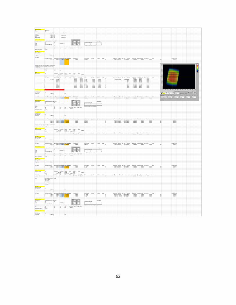
62
beam conditionstest DRBugsA1-R1camera DS-1camera mag 9.6 err 0.1 µm/pxovl pulse 6.00E+01 µsarea pulse 1.60E+02 µs 5.93E-04 cm2area 7.98E-02 errbeam current 6.00E+01 err 3.00E+00 nA
device conditionsDRBugsA1-R1 multiple positions on row 1,3,5,7 marking locnIe n/a uA Die matrix location #stemp RT K no control on 3 2 1posn first one on the left 6 5 4M2 thk µm very thin bottom strip not exposedVBB VRB VEE VCC VRC VBC = (VCC - |VRC|) – (VBB - |VRB|)
n/a n/a n/a n/a #VALUE!Set A, Plate 1, Row 1 to start
test shotsDRBugsA1-R1testTIA - K428 gain test #charge state 1.00E+06 V/A
1test shot#
0 device fluence /cm2 avg fluence targ pulse (nom) pulse target (sec) TIA gain (V/A) pulse (meas) k_fact(1) k_fact(n) index avg fluence avg fl err dev fl err pulse err pulse (calc) fluence/us error calc fl/us err freq dev/avg fl ratio1.12E+10 7.20E+09 1.600E-03 1.584E-03 1.00E+08 1.59999m 0 7.27E+09 2.62E+08 7.14E+08 13.95u 1.6000E-03 0.000% 0.000% 100 1.54E+00
New code puts single pulse on each scan matrix element.use test fluence on eac well before exposure serieswells 1 thru 8
well 1 shot 0well 2 shot 1 etc
SHOTDRBugsA1-R1 _# irradiation 4x3 matrix Xstep 2mm ystep 3mm
H 4.5 MeV charge 1 gain 1.00E+06W# Pulse 1.665E-02 sec target fluenc 7.20E+10 /cm2
Shot Fluence Total Fluence VRB VRC VRE Gain delta(1/G) Pulse k_fact(1) k_fact(n) index avg fluence avg fl err dev fl err pulse err pulse (calc) fluence/us error calc fl/us err note0 #DIV/0! #DIV/0! 0 #VALUE! #DIV/0! #DIV/0!
1 1.12E+10 1.12E+10 #DIV/0! #DIV/0! 14.548m #DIV/0! #VALUE! 1 7.27E+09 2.62E+08 7.14E+08 13.95u 1.4548E-02 #DIV/0! #DIV/0!2 1.12E+10 #DIV/0! #DIV/0! 14.548m #DIV/0! #VALUE! 2 308.4u 1.4548E-02 #DIV/0! #DIV/0!3 1.12E+10 #DIV/0! #DIV/0! 14.7731m #DIV/0! #VALUE! 3 308.4u 1.4773E-02 #DIV/0! #DIV/0!4 1.12E+10 #DIV/0! #DIV/0! 14.7731m #DIV/0! #VALUE! 4 308.4u 1.4773E-02 #DIV/0! #DIV/0!5 1.12E+10 #DIV/0! #DIV/0! 14.7731m #DIV/0! #VALUE! 5 308.4u 1.4773E-02 #DIV/0! #DIV/0!6 1.12E+10 #DIV/0! #DIV/0! 14.7731m #DIV/0! #VALUE! 6 308.4u 1.4773E-02 #DIV/0! #DIV/0!7 1.12E+10 #DIV/0! #DIV/0! 14.7731m #DIV/0! #VALUE! 7 308.4u 1.4773E-02 #DIV/0! #DIV/0!8 1.12E+10 #DIV/0! #DIV/0! 14.7169m #DIV/0! #VALUE! 8 155.4u 1.4717E-02 #DIV/0! #DIV/0!
test shots FILES NOT SAVED!!!!! - see next test shot _0DRBugsA1-R1W8TIA - K428 gain test #charge state 1.00E+06 V/A
1
test shot# device fluence /cm2 avg fluence targ pulse (nom) pulse target (sec) TIA gain (V/A) pulse (meas) k_fact(1) k_fact(n) index avg fluence avg fl err dev fl err pulse err pulse (calc) fluence/us error calc fl/us err freq dev/avg fl ratio0 1.12E+10 7.20E+09 1.600E-03 1.584E-03 1.00E+08 1.59999m 0 7.27E+09 2.62E+08 7.14E+08 13.95u 1.6000E-03 0.000% 0.000% 100 1.54E+00
device conditionsDRBugsA1-R3 multiple positions on row 1,3,5,7 marking locnIe n/a uA Die matrix location #stemp RT K no control on 3 2 1posn first one on the left 6 5 4M2 thk µm very thin bottom strip not exposedVBB VRB VEE VCC VRC VBC = (VCC - |VRC|) – (VBB - |VRB|)
n/a n/a n/a n/a #VALUE!Set A, Plate 1, Row 3 to start
test shotsDRBugsA1-R3testTIA - K428 gain test #charge state 1.00E+06 V/A
1
test shot# device fluence /cm2 avg fluence targ pulse (nom) pulse target (sec) TIA gain (V/A) pulse (meas) k_fact(1) k_fact(n) index avg fluence avg fl err dev fl err pulse err pulse (calc) fluence/us error calc fl/us err freq dev/avg fl ratio0 1.07E+10 3.60E+10 1.600E-03 8.273E-03 1.00E+08 1.59252m 0 6.96E+09 2.29E+08 7.14E+08 12.03u 1.5925E-03 0.000% 0.000% 100 1.54E+001 5.90E+10 3.60E+10 8.270E+03 7.773E+03 1.00E+08 8.26544m 0 3.83E+10 1.18E+09 3.59E+09 16.69u 8.2654E-03 0.000% 0.000% 100 1.54E+002 5.90E+10 3.60E+10 7.800E+00 7.332E+00 1.00E+08 8.26544m 0 3.83E+10 1.18E+09 3.59E+09 16.69u 8.2654E-03 0.000% 0.000% 100 1.54E+00
New code puts single pulse on each scan matrix element.use test fluence ffor all following shots.
SHOTDRBugsA1-R3W# _# irradiation 4x3 matrix Xstep 2mm ystep 3mm
H 4.5 MeV charge 1 gain 1.00E+06Pulse 7.800E-03 sec target fluenc 3.60E+10 /cm2
shot # Shot Fluence Total Fluence VRB VRC VRE Gain delta(1/G) Pulse k_fact(1) k_fact(n) index avg fluence avg fl err dev fl err pulse err pulse (calc) fluence/us error calc fl/us err notewells1 thru 8 0 #DIV/0! #DIV/0! 0 #VALUE! #DIV/0! #DIV/0!
test shotsDRBugsA1-R3W8TIA - K428 gain test #charge state 1.00E+06 V/A
1
test shot# device fluence /cm2 avg fluence targ pulse (nom) pulse target (sec) TIA gain (V/A) pulse (meas) k_fact(1) k_fact(n) index avg fluence avg fl err dev fl err pulse err pulse (calc) fluence/us error calc fl/us err freq dev/avg fl ratio0 5.44E+10 3.60E+10 7.800E-03 7.950E-03 1.00E+08 7.80174m 0 3.53E+10 9.71E+08 3.23E+09 21.25u 7.8017E-03 0.000% 0.000% 100 1.54E+00
device conditionsDRBugsA1-R5 multiple positions on row 1,3,5,7 marking locnIe n/a uA Die matrix location #stemp RT K no control on 3 2 1posn first one on the left 6 5 4M2 thk µm very thin bottom strip not exposedVBB VRB VEE VCC VRC VBC = (VCC - |VRC|) – (VBB - |VRB|)
n/a n/a n/a n/a #VALUE!Set A, Plate 1, Row 5 to start
test shotsDRBugsA1-R5testTIA - K428 gain test #charge state 1.00E+06 V/A
1
test shot# device fluence /cm2 avg fluence targ pulse (nom) pulse target (sec) TIA gain (V/A) pulse (meas) k_fact(1) k_fact(n) index avg fluence avg fl err dev fl err pulse err pulse (calc) fluence/us error calc fl/us err freq dev/avg fl ratio0 1.04E+11 7.20E+10 1.590E-02 1.702E-02 1.00E+08 16.3248m 0 6.73E+10 2.79E+09 6.94E+09 389.8u 1.6325E-02 0.000% 0.000% 100 1.54E+001 1.10E+11 7.20E+10 1.590E-02 1.603E-02 1.00E+08 16.9839m 0 7.14E+10 4.43E+09 8.94E+09 545.5u 1.6984E-02 0.000% 0.000% 100 1.54E+00
SHOTDRBugsA1-R5W# _# irradiation 4x3 matrix Xstep 2mm ystep 3mm
H 4.5 MeV charge 1 gain 1.00E+06Pulse 7.800E-03 sec target fluenc 3.60E+10 /cm2
shot # Shot Fluence Total Fluence VRB VRC VRE Gain delta(1/G) Pulse k_fact(1) k_fact(n) index avg fluence avg fl err dev fl err pulse err pulse (calc) fluence/us error calc fl/us err notewells1 thru 8 0 #DIV/0! #DIV/0! 0 #VALUE! #DIV/0! #DIV/0!
note insim keeps messing file savingwells 1,2 savedwells 3,4 lostcode restartedwells 5, 6, 7 savedwell 8 lost
test shotsDRBugsA1-R5W8TIA - K428 gain test #charge state 1.00E+06 V/A
1
test shot# device fluence /cm2 avg fluence targ pulse (nom) pulse target (sec) TIA gain (V/A) pulse (meas) k_fact(1) k_fact(n) index avg fluence avg fl err dev fl err pulse err pulse (calc) fluence/us error calc fl/us err freq dev/avg fl ratio0 1.04E+11 1.80E+11 1.590E-02 4.256E-02 1.00E+08 16.3248m 0 6.73E+10 2.79E+09 6.94E+09 389.8u 1.6325E-02 0.000% 0.000% 100 1.54E+001 1.04E+11 1.80E+11 1.590E-02 4.276E-02 1.00E+08 16.1579m 0 6.69E+10 2.56E+09 6.69E+09 229.6u 1.6158E-02 0.000% 0.000% 100 1.55E+002 1.04E+11 1.80E+11 1.590E-02 4.276E-02 1.00E+08 16.1579m 0 6.69E+10 2.56E+09 6.69E+09 229.6u 1.6158E-02 0.000% 0.000% 100 1.55E+00
device conditionsDRBugsA1-R7 multiple positions on row 1,3,5,7 marking locnIe n/a uA Die matrix location #stemp RT K no control on 3 2 1posn first one on the left 6 5 4M2 thk µm very thin bottom strip not exposedVBB VRB VEE VCC VRC VBC = (VCC - |VRC|) – (VBB - |VRB|)
n/a n/a n/a n/a #VALUE!Set A, Plate 1, Row 7 to start
test shotsDRBugsA1-R7testTIA - K428 gain test #charge state 1.00E+06 V/A
1
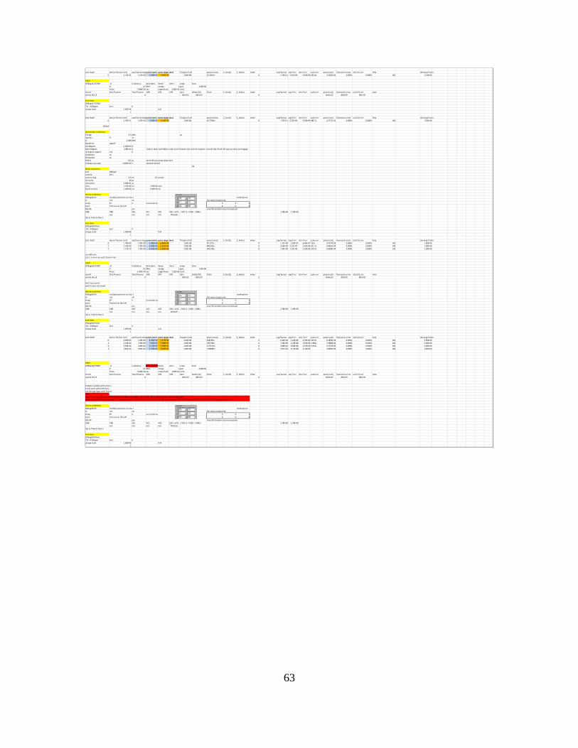
63
test shot# device fluence /cm2 avg fluence targepulse (nom) pulse target (sec) TIA gain (V/A) pulse (meas) k_fact(1) k_fact(n) index avg fluence avg fl err dev fl err pulse err pulse (calc) fluence/us error calc fl/us err freq dev/avg fl ratio0 2.71E+11 1.67E+10 1.590E-02 1.507E-03 1.00E+08 42.5654m 0 1.76E+11 5.65E+09 6.94E+09 235.8u 4.2565E-02 0.000% 0.000% 100 1.54E+00
SHOTDRBugsA1-R7W# _# irradiation 4x3 matrix Xstep 2mm ystep 3mm
H 4.5 MeV charge 1 gain 1.00E+06Pulse 7.800E-03 sec target fluenc 3.60E+10 /cm2
shot # Shot Fluence Total Fluence VRB VRC VRE Gain delta(1/G) Pulse k_fact(1) k_fact(n) index avg fluence avg fl err dev fl err pulse err pulse (calc) fluence/us error calc fl/us err notewells1 thru 8 0 #DIV/0! #DIV/0! 0 #VALUE! #DIV/0! #DIV/0!
test shotsDRBugsA1-R7W8TIA - K428 gain test #charge state 1.00E+06 V/A
1
test shot# device fluence /cm2 avg fluence targepulse (nom) pulse target (sec) TIA gain (V/A) pulse (meas) k_fact(1) k_fact(n) index avg fluence avg fl err dev fl err pulse err pulse (calc) fluence/us error calc fl/us err freq dev/avg fl ratio0 2.70E+11 1.67E+10 1.590E-02 1.515E-03 1.00E+08 42.7706m 0 1.75E+11 5.72E+09 6.94E+09 385.7u 4.2771E-02 0.000% 0.000% 100 1.54E+00
170119
Accelerator conditionsEnergy 4.5 MeV apSpecies H 1+tv 2.289 MeVBeamline qaspr3Ext Magnet -1.00E+03 GMain Magnet 4.08E-02 G Tried to steer with MM in order to shift beam over with Ext magnet, since BL Obj slit all the way out does not engage.45 degree magnet n/a GLE Blanker onHE Blanker onBHE bl 4.25 µs set to 30 usec pulse alignmentfaraday cup suppr 2.606E+02 V checked 161122
Apbeam conditionstest DRBugs!camera DS-1camera mag 9.6 err 0.1 µm/pxovl pulse 20 µsarea pulse 6.00E+01 µsarea 7.51E-02 err 7.91E-04 cm2beam current 1.20E+02 err 3.00E+00 nA
device conditionsDRbugA8-R1 multiple positions on row 1 marking locnIe n/a uA Die matrix location #stemp RT K no control on 3 2 1posn first one on the left 6 5 4M2 thk µm very thin bottom strip not exposedVBB VRB VEE VCC VRC VBC = (VCC - |VRC|) – (VBB - |VRB|) 1.78E+09 1.78E+09
n/a n/a n/a n/a #VALUE!Set A, Plate 8, Row 1
test shotsDRbugA8-R1testTIA - K428 gain test #charge state 1.00E+06 V/A
1
test shot# device fluence /cm2 avg fluence targepulse (nom) pulse target (sec) TIA gain (V/A) pulse (meas) k_fact(1) k_fact(n) index avg fluence avg fl err dev fl err pulse err pulse (calc) fluence/us error calc fl/us err freq dev/avg fl ratio0 1.78E+09 7.20E+09 1.000E-04 6.481E-04 1.00E+08 99.1771u 0 1.11E+09 2.28E+07 8.40E+07 133n 9.9177E-05 0.000% 0.000% 100 1.60E+001 7.33E+09 7.20E+09 4.056E-04 6.361E-04 1.00E+08 404.813u 0 4.59E+09 9.12E+07 3.45E+08 422.1n 4.0481E-04 0.000% 0.000% 100 1.60E+002 1.17E+10 7.20E+09 6.420E-04 6.300E-04 1.00E+08 640.976u 0 7.34E+09 1.19E+08 5.34E+08 379.5n 6.4098E-04 0.000% 0.000% 100 1.60E+00
use 630 usecuse 2.1 mm x incr and 2.9 mm Y incr
SHOTDRBugsA8-R1W# _# irradiation 4x3 matrix Xstep 2mm ystep 3mm
H 4.5 MeV charge 1 gain 1.00E+06Pulse 6.300E-04 sec target fluenc 7.20E+09 /cm2
shot # Shot Fluence Total Fluence VRB VRC VRE Gain delta(1/G) Pulse k_fact(1) k_fact(n) index avg fluence avg fl err dev fl err pulse err pulse (calc) fluence/us error calc fl/us err notewells1 thru 8 0 #DIV/0! #DIV/0! 0 #VALUE! #DIV/0! #DIV/0!
well 1 pic savedwell 2-3 pics not saved
device conditionsDRbugA8-R3 multiple positions on row 1 marking locnIe n/a uA Die matrix location #stemp RT K no control on 3 2 1posn first one on the left 6 5 4M2 thk µm very thin bottom strip not exposedVBB VRB VEE VCC VRC VBC = (VCC - |VRC|) – (VBB - |VRB|) 1.78E+09 1.78E+09
n/a n/a n/a n/a #VALUE!Set A, Plate 8, Row 3
test shotsDRbugA8-R1testTIA - K428 gain test #charge state 1.00E+06 V/A
1
test shot# device fluence /cm2 avg fluence targepulse (nom) pulse target (sec) TIA gain (V/A) pulse (meas) k_fact(1) k_fact(n) index avg fluence avg fl err dev fl err pulse err pulse (calc) fluence/us error calc fl/us err freq dev/avg fl ratio0 9.96E+09 7.20E+09 6.300E-04 7.275E-04 1.00E+08 628.905u 0 6.24E+09 1.26E+08 4.70E+08 313.9n 6.2891E-04 0.000% 0.000% 100 1.60E+001 1.14E+10 7.20E+09 7.250E-05 7.289E-05 1.00E+08 726.799u 0 7.16E+09 1.22E+08 5.25E+08 1.284u 7.2680E-04 0.000% 0.000% 100 1.60E+002 4.93E+10 3.60E+10 3.170E-03 3.700E-03 1.00E+08 3.17174m 0 3.08E+10 6.84E+08 2.37E+09 5.041u 3.1717E-03 0.000% 0.000% 100 1.60E+003 5.85E+10 3.60E+10 3.700E-03 3.634E-03 1.00E+08 3.69848m 0 3.67E+10 6.71E+08 2.72E+09 3.6985E-03 0.000% 0.000% 100 1.60E+00
SHOTDRBugsA8-R3W# _# irradiation 4x3 matrix***Xstep 2mm ystep 3mm
H 4.5 MeV charge 1 gain 1.00E+06Pulse 3.630E-03 sec target fluenc 3.60E+10 /cm2
shot # Shot Fluence Total Fluence VRB VRC VRE Gain delta(1/G) Pulse k_fact(1) k_fact(n) index avg fluence avg fl err dev fl err pulse err pulse (calc) fluence/us error calc fl/us err notewells1 thru 8 0 #DIV/0! #DIV/0! 0 #VALUE! #DIV/0! #DIV/0!
forgot to update pulse times!hit all wells with 0.63 msecran through again with 3 msec***On well 4 it was discovered that the beam width was 1.9 mm, not 2.1 mm. So 2.1 mm step size was leaving a gap.So for wells 4-8 the scan settings were changed to a 5 x 3 matrix and the left and right edges were allowed to extend out a little further towards the neighbouring wells.
device conditionsDRbugA8-R5 multiple positions on row 1 marking locnIe n/a uA Die matrix location #stemp RT K no control on 3 2 1posn first one on the left 6 5 4M2 thk µm very thin bottom strip not exposedVBB VRB VEE VCC VRC VBC = (VCC - |VRC|) – (VBB - |VRB|) 1.78E+09 1.78E+09
n/a n/a n/a n/a #VALUE!Set A, Plate 8, Row 5
test shotsDRbugA8-R5testTIA - K428 gain test #charge state 1.00E+06 V/A
1
64
test shot# device fluence /cm2 avg fluence targepulse (nom) pulse target (sec) TIA gain (V/A) pulse (meas) k_fact(1) k_fact(n) index avg fluence avg fl err dev fl err pulse err pulse (calc) fluence/us error calc fl/us err freq dev/avg fl ratio0 9.74E+10 7.20E+10 7.270E-03 8.581E-03 1.00E+08 7.25906m 0 6.10E+10 1.36E+09 4.68E+09 31.22u 7.2591E-03 0.000% 0.000% 100 1.60E+001 1.16E+11 7.20E+10 8.580E+00 8.546E+00 1.00E+08 8.57231m 0 7.23E+10 1.54E+09 5.50E+09 10.07u 8.5723E-03 0.000% 0.000% 100 1.60E+00
SHOTDRBugsA8-R5W# _# irradiation 5x3 matrix Xstep 1.9 ystep 2.9
H 4.5 MeV charge 1 gain 1.00E+06Pulse 8.550E-03 sec target fluenc 7.20E+10 /cm2
shot # Shot Fluence Total Fluence VRB VRC VRE Gain delta(1/G) Pulse k_fact(1) k_fact(n) index avg fluence avg fl err dev fl err pulse err pulse (calc) fluence/us error calc fl/us err notewells1 thru 8 0 #DIV/0! #DIV/0! 0 #VALUE! #DIV/0! #DIV/0!
test shotsDRbugA8-R5W8TIA - K428 gain test #charge state 1.00E+06 V/A
1
test shot# device fluence /cm2 avg fluence targepulse (nom) pulse target (sec) TIA gain (V/A) pulse (meas) k_fact(1) k_fact(n) index avg fluence avg fl err dev fl err pulse err pulse (calc) fluence/us error calc fl/us err freq dev/avg fl ratio0 1.07E+11 7.20E+10 8.580E+00 9.194E+00 1.00E+08 8.58599m 0 6.72E+10 1.80E+09 5.40E+09 33.82u 8.5860E-03 0.000% 0.000% 100 1.60E+00
device conditionsDRbugA8-R7 multiple positions on row 1 marking locnIe n/a uA Die matrix location #stemp RT K no control on 3 2 1posn first one on the left 6 5 4M2 thk µm very thin bottom strip not exposedVBB VRB VEE VCC VRC VBC = (VCC - |VRC|) – (VBB - |VRB|) 1.78E+09 1.78E+09
n/a n/a n/a n/a #VALUE!Set A, Plate 8, Row 7
test shotsDRbugA8-R5W8TIA - K428 gain test #charge state 1.00E+06 V/A
1
test shot# device fluence /cm2 avg fluence targepulse (nom) pulse target (sec) TIA gain (V/A) pulse (meas) k_fact(1) k_fact(n) index avg fluence avg fl err dev fl err pulse err pulse (calc) fluence/us error calc fl/us err freq dev/avg fl ratio0 2.87E+11 1.80E+11 2.300E-02 2.308E-02 1.00E+08 23.1275m 0 1.79E+11 4.64E+09 1.43E+10 185.9u 2.3128E-02 0.000% 0.000% 100 1.60E+00
SHOTDRBugsA8-R7W# _# irradiation 5x3 matrix Xstep 1.9 ystep 2.9
H 4.5 MeV charge 1 gain 1.00E+06Pulse 2.300E-02 sec target fluenc 1.80E+11 /cm2
shot # Shot Fluence Total Fluence VRB VRC VRE Gain delta(1/G) Pulse k_fact(1) k_fact(n) index avg fluence avg fl err dev fl err pulse err pulse (calc) fluence/us error calc fl/us err notewells1 thru 8 0 #DIV/0! #DIV/0! 0 #VALUE! #DIV/0! #DIV/0!
post shot beam check upon loading of B1 plate red show original beam spot outline
possibly quad got bumped when we were trying to figure out the matrix to use.area calc was 8.2e-2 cm2
beam conditionstest DRBugs!camera DS-1camera mag 9.6 err 0.1 µm/pxovl pulse 20 µsarea pulse 6.00E+01 µsarea 8.84E-02 err 9.32E-04 cm2beam current 7.80E+01 err 3.00E+00 nA
device conditionsDRbugB1-R1 multiple positions on row 1 marking locnIe n/a uA Die matrix location #stemp RT K no control on 3 2 1posn first one on the left 6 5 4M2 thk µm very thin bottom strip not exposedVBB VRB VEE VCC VRC VBC = (VCC - |VRC|) – (VBB - |VRB|) 1.78E+09 1.78E+09
n/a n/a n/a n/a #VALUE!Set B, Plate 1, Row 1
test shotsDRbugB1-R1testTIA - K428 gain test #charge state 1.00E+06 V/A
1
test shot# device fluence /cm2 avg fluence targepulse (nom) pulse target (sec) TIA gain (V/A) pulse (meas) k_fact(1) k_fact(n) index avg fluence avg fl err dev fl err pulse err pulse (calc) fluence/us error calc fl/us err freq dev/avg fl ratio0 8.29E+08 7.20E+08 1.000E-04 1.344E-04 1.00E+08 99.1321u 0 5.36E+08 1.20E+07 4.08E+07 152.8n 9.9132E-05 0.000% 0.000% 100 1.55E+001 1.13E+09 7.20E+08 1.344E-04 1.329E-04 1.00E+08 133.311u 0 7.28E+08 1.50E+07 5.45E+07 109.2n 1.3331E-04 0.000% 0.000% 100 1.55E+00
SHOTDRbugB1-R1W1 _# irradiation 4x3 Xstep 2.15 ystep 3.1
H 4.5 MeV charge 1 gain 1.00E+06Pulse 1.330E-04 sec target fluenc 7.20E+08 /cm2
shot # Shot Fluence Total Fluence VRB VRC VRE Gain delta(1/G) Pulse k_fact(1) k_fact(n) index avg fluence avg fl err dev fl err pulse err pulse (calc) fluence/us error calc fl/us err notewells1 thru 8 0 #DIV/0! #DIV/0! 0 #VALUE! #DIV/0! #DIV/0!
lost well 5 picsprobaly the beam line valve was closed for wells 5, 6, 7, and 8
device conditionsDRbugB1-R3 multiple positions on row 1 marking locnIe n/a uA Die matrix location #stemp RT K no control on 3 2 1posn first one on the left 6 5 4M2 thk µm very thin bottom strip not exposedVBB VRB VEE VCC VRC VBC = (VCC - |VRC|) – (VBB - |VRB|) 1.78E+09 1.78E+09
n/a n/a n/a n/a #VALUE!Set B, Plate 1, Row 7
checked beam posn on phosphor - looks good
test shotsDRbugB1-R7testTIA - K428 gain test #charge state 1.00E+06 V/A
1
test shot# device fluence /cm2 avg fluence targepulse (nom) pulse target (sec) TIA gain (V/A) pulse (meas) k_fact(1) k_fact(n) index avg fluence avg fl err dev fl err pulse err pulse (calc) fluence/us error calc fl/us err freq dev/avg fl ratio0 1.08E+11 7.20E+11 1.330E+01 1.376E+02 1.00E+08 13.3889m 0 6.96E+10 1.65E+09 5.45E+07 36.43u 1.3389E-02 0.000% 0.000% 100 1.55E+001 1.06E+11 7.20E+11 1.380E+01 1.449E+02 1.00E+08 13.8871m 0 6.86E+10 1.99E+09 5.57E+09 48.35u 1.3887E-02 0.000% 0.000% 100 1.55E+002 1.13E+11 7.20E+11 1.450E-02 1.425E-01 1.00E+08 14.5792m 0 7.33E+10 2.15E+09 5.98E+09 150.8u 1.4579E-02 0.000% 0.000% 100 1.55E+00
Actual fluence 10 times higher Use Scaled pulse time 10X
SHOTDRbugB1-R7W1 _# irradiation 4x3 Xstep 2.15 ystep 3.1
H 4.5 MeV charge 1 gain 1.00E+06Pulse 1.425E-01 sec target fluenc 7.20E+11 /cm2
shot # Shot Fluence Total Fluence VRB VRC VRE Gain delta(1/G) Pulse k_fact(1) k_fact(n) index avg fluence avg fl err dev fl err pulse err pulse (calc) fluence/us error calc fl/us err notewells1 thru 8 0 #DIV/0! #DIV/0! 0 #VALUE! #DIV/0! #DIV/0!
2 extra pulse in well 1 in the center; no pics; no visible damage
test shot# device fluence /cm2 avg fluence targepulse (nom) pulse target (sec) TIA gain (V/A) pulse (meas) k_fact(1) k_fact(n) index avg fluence avg fl err dev fl err pulse err pulse (calc) fluence/us error calc fl/us err freq dev/avg fl ratio0 1.14E+11 7.20E+11 1.450E+01 1.421E+02 1.00E+08 14.6117m 0 7.35E+10 1.51E+09 5.45E+07 205.3u 1.4612E-02 0.000% 0.000% 100 1.55E+00
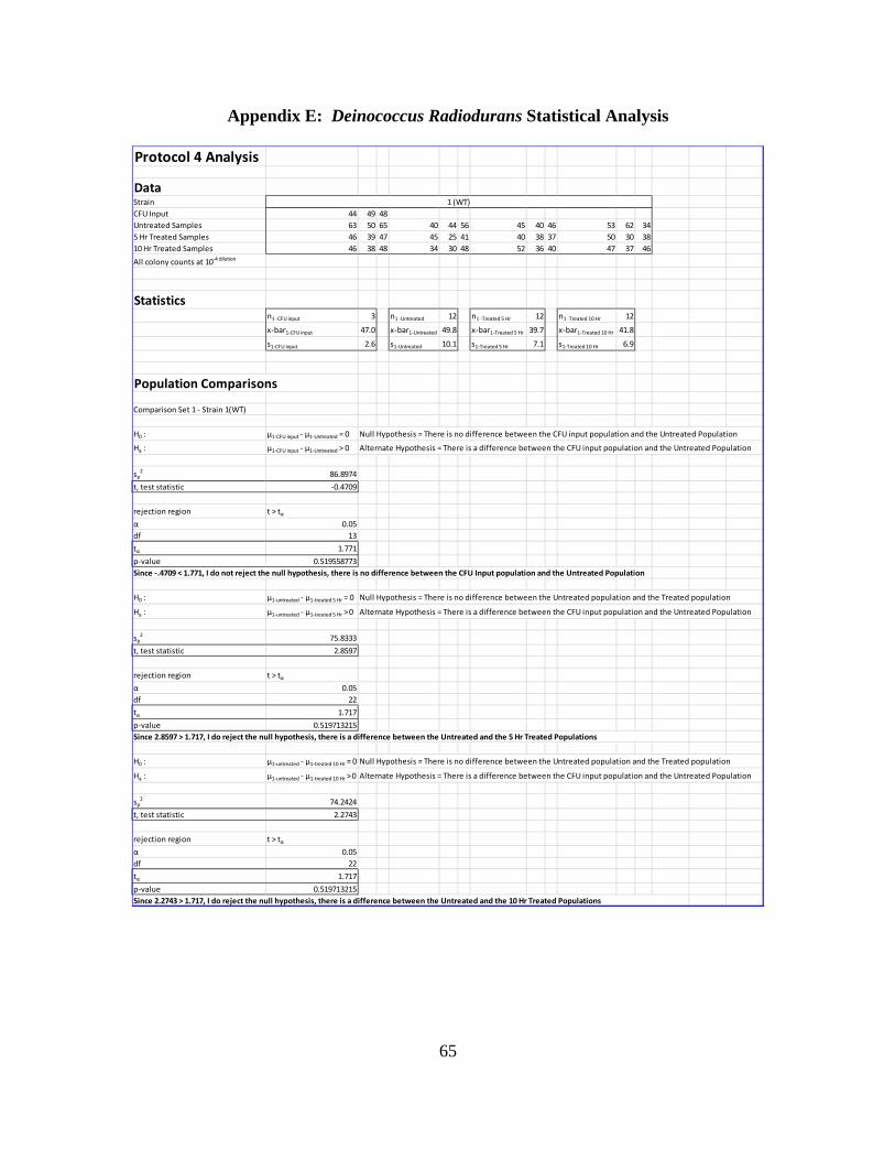
65
Appendix E: Deinococcus Radiodurans Statistical Analysis
Protocol 4 Analysis
DataStrainCFU Input 44 49 48Untreated Samples 63 50 65 40 44 56 45 40 46 53 62 345 Hr Treated Samples 46 39 47 45 25 41 40 38 37 50 30 3810 Hr Treated Samples 46 38 48 34 30 48 52 36 40 47 37 46All colony counts at 10-4 dilution
Statisticsn1 -CFU input 3 n1 -Untreated 12 n1 -Treated 5 Hr 12 n1 -Treated 10 Hr 12
x-bar1-CFU input 47.0 x-bar1-Untreated 49.8 x-bar1-Treated 5 Hr 39.7 x-bar1-Treated 10 Hr 41.8
s1-CFU input 2.6 s1-Untreated 10.1 s1-Treated 5 Hr 7.1 s1-Treated 10 Hr 6.9
Population Comparisons
Comparison Set 1 - Strain 1(WT)
H0 : µ1-CFU input - µ1-Untreated = 0
Ha : µ1-CFU input - µ1-Untreated > 0
sp2 86.8974
t, test statistic -0.4709
rejection region t > tα
α 0.05df 13tα 1.771p-value 0.519558773
H0 : µ1-untreated - µ1-treated 5 Hr = 0
Ha : µ1-untreated - µ1-treated 5 Hr > 0
sp2 75.8333
t, test statistic 2.8597
rejection region t > tα
α 0.05df 22tα 1.717p-value 0.519713215
H0 : µ1-untreated - µ1-treated 10 Hr = 0
Ha : µ1-untreated - µ1-treated 10 Hr > 0
sp2 74.2424
t, test statistic 2.2743
rejection region t > tα
α 0.05df 22tα 1.717p-value 0.519713215
Since 2.8597 > 1.717, I do reject the null hypothesis, there is a difference between the Untreated and the 5 Hr Treated Populations
Null Hypothesis = There is no difference between the Untreated population and the Treated population
Alternate Hypothesis = There is a difference between the CFU input population and the Untreated Population
Since 2.2743 > 1.717, I do reject the null hypothesis, there is a difference between the Untreated and the 10 Hr Treated Populations
1 (WT)
Null Hypothesis = There is no difference between the CFU input population and the Untreated Population
Alternate Hypothesis = There is a difference between the CFU input population and the Untreated Population
Null Hypothesis = There is no difference between the Untreated population and the Treated population
Alternate Hypothesis = There is a difference between the CFU input population and the Untreated Population
Since -.4709 < 1.771, I do not reject the null hypothesis, there is no difference between the CFU Input population and the Untreated Population
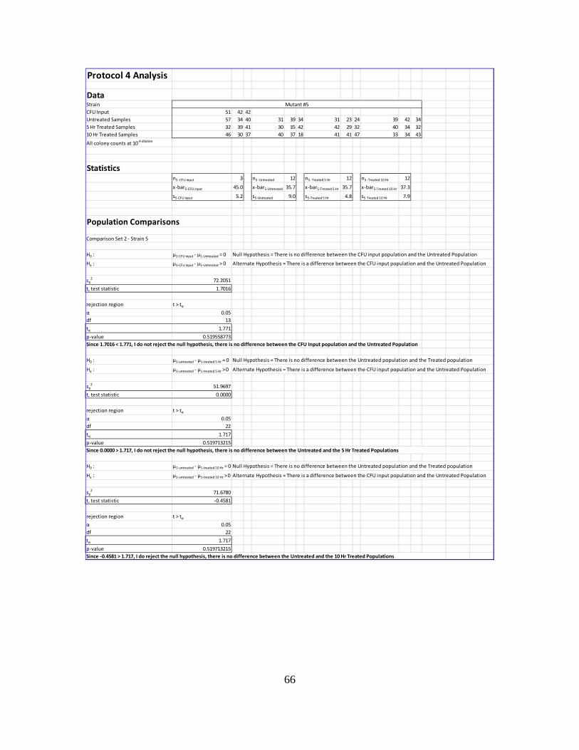
66
Protocol 4 Analysis
DataStrainCFU Input 51 42 42Untreated Samples 57 34 40 31 39 34 31 23 24 39 42 345 Hr Treated Samples 32 39 41 30 35 42 42 29 32 40 34 3210 Hr Treated Samples 46 30 37 40 37 18 41 41 47 33 34 43All colony counts at 10-4 dilution
Statisticsn5 -CFU input 3 n5 -Untreated 12 n5 -Treated 5 Hr 12 n5 -Treated 10 Hr 12
x-bar5-CFU input 45.0 x-bar5-Untreated 35.7 x-bar5-Treated 5 Hr 35.7 x-bar5-Treated 10 Hr 37.3
s5-CFU input 5.2 s5-Untreated 9.0 s5-Treated 5 Hr 4.8 s5-Treated 10 Hr 7.9
Population Comparisons
Comparison Set 2 - Strain 5
H0 : µ1-CFU input - µ1-Untreated = 0
Ha : µ1-CFU input - µ1-Untreated > 0
sp2 72.2051
t, test statistic 1.7016
rejection region t > tα
α 0.05df 13tα 1.771p-value 0.519558773
H0 : µ1-untreated - µ1-treated 5 Hr = 0
Ha : µ1-untreated - µ1-treated 5 Hr > 0
sp2 51.9697
t, test statistic 0.0000
rejection region t > tα
α 0.05df 22tα 1.717p-value 0.519713215
H0 : µ1-untreated - µ1-treated 10 Hr = 0
Ha : µ1-untreated - µ1-treated 10 Hr > 0
sp2 71.6780
t, test statistic -0.4581
rejection region t > tα
α 0.05df 22tα 1.717p-value 0.519713215
Null Hypothesis = There is no difference between the Untreated population and the Treated population
Mutant #5
Null Hypothesis = There is no difference between the CFU input population and the Untreated Population
Alternate Hypothesis = There is a difference between the CFU input population and the Untreated Population
Since 1.7016 < 1.771, I do not reject the null hypothesis, there is no difference between the CFU Input population and the Untreated Population
Alternate Hypothesis = There is a difference between the CFU input population and the Untreated Population
Since 0.0000 > 1.717, I do not reject the null hypothesis, there is no difference between the Untreated and the 5 Hr Treated Populations
Null Hypothesis = There is no difference between the Untreated population and the Treated population
Alternate Hypothesis = There is a difference between the CFU input population and the Untreated Population
Since -0.4581 > 1.717, I do reject the null hypothesis, there is no difference between the Untreated and the 10 Hr Treated Populations

67
Protocol 4 Analysis
DataStrainCFU Input 43 58 42Untreated Samples 58 43 42 38 25 28 26 26 41 33 45 445 Hr Treated Samples 48 46 39 37 39 37 45 54 41 67 35 3410 Hr Treated Samples 26 26 31 30 43 28 37 33 31 26 39 36All colony counts at 10-4 dilution
Statisticsn8 -CFU input 3 n8 -Untreated 12 n8 -Treated 5 Hr 12 n8 -Treated 10 Hr 12
x-bar8-CFU input 47.7 x-bar8-Untreated 37.4 x-bar8-Treated 5 Hr 43.5 x-bar8-Treated 10 Hr 32.2
s8-CFU input 9.0 s8-Untreated 10.1 s8-Treated 5 Hr 9.5 s8-Treated 10 Hr 5.6
Population Comparisons
Comparison Set 3 - Strain 8
H0 : µ1-CFU input - µ1-Untreated = 0
Ha : µ1-CFU input - µ1-Untreated > 0
sp2 97.9679
t, test statistic 1.6043
rejection region t > tα
α 0.05df 13tα 1.771p-value 0.519558773
H0 : µ1-untreated - µ1-treated 5 Hr = 0
Ha : µ1-untreated - µ1-treated 5 Hr > 0
sp2 95.3598
t, test statistic -1.5259
rejection region t > tα
α 0.05df 22tα 1.717p-value 0.519713215
H0 : µ1-untreated - µ1-treated 10 Hr = 0
Ha : µ1-untreated - µ1-treated 10 Hr > 0
sp2 66.1174
t, test statistic 1.5815
rejection region t > tα
α 0.05df 22tα 1.717p-value 0.519713215
Null Hypothesis = There is no difference between the Untreated population and the Treated population
Mutant #8
Null Hypothesis = There is no difference between the CFU input population and the Untreated Population
Alternate Hypothesis = There is a difference between the CFU input population and the Untreated Population
Since 1.6043 < 1.771, I do not reject the null hypothesis, there is no difference between the CFU Input population and the Untreated Population
Alternate Hypothesis = There is a difference between the CFU input population and the Untreated Population
Since -1.5259 > 1.717, I do not reject the null hypothesis, there is no difference between the Untreated and the 5 Hr Treated Populations
Null Hypothesis = There is no difference between the Untreated population and the Treated population
Alternate Hypothesis = There is a difference between the CFU input population and the Untreated Population
Since 1.5815 > 1.717, I do reject the null hypothesis, there is no difference between the Untreated and the 10 Hr Treated Populations

68
Protocol 4 Analysis
DataStrainCFU Input 37 37 38Untreated Samples 43 30 32 42 21 32 30 25 21 32 20 335 Hr Treated Samples 31 31 26 28 42 44 38 37 29 47 40 2110 Hr Treated Samples 44 36 34 38 42 44 39 46 38 42 40 33All colony counts at 10-4 dilution
Statisticsn11 -CFU input 3 n11 -Untreated 12 n11 -Treated 5 Hr 12 n11 -Treated 10 Hr 12
x-bar11-CFU input 37.3 x-bar11-Untreated 30.1 x-bar11-Treated 5 Hr 34.5 x-bar11-Treated 10 Hr 39.7
s11-CFU input 0.6 s11-Untreated 7.5 s11-Treated 5 Hr 8.0 s11-Treated 10 Hr 4.1
Population Comparisons
Comparison Set 4 - Strain 11
H0 : µ1-CFU input - µ1-Untreated = 0
Ha : µ1-CFU input - µ1-Untreated > 0
sp2 47.8141
t, test statistic 1.6243
rejection region t > tα
α 0.05df 13tα 1.771p-value 0.519558773
H0 : µ1-untreated - µ1-treated 5 Hr = 0
Ha : µ1-untreated - µ1-treated 5 Hr > 0
sp2 60.1780
t, test statistic -1.3946
rejection region t > tα
α 0.05df 22tα 1.717p-value 0.519713215
H0 : µ1-untreated - µ1-treated 10 Hr = 0
Ha : µ1-untreated - µ1-treated 10 Hr > 0
sp2 36.6174
t, test statistic -3.8793
rejection region t > tα
α 0.05df 22tα 1.717p-value 0.519713215
Null Hypothesis = There is no difference between the Untreated population and the Treated population
Mutant #11
Null Hypothesis = There is no difference between the CFU input population and the Untreated Population
Alternate Hypothesis = There is a difference between the CFU input population and the Untreated Population
Since 1.6243 < 1.771, I do not reject the null hypothesis, there is no difference between the CFU Input population and the Untreated Population
Alternate Hypothesis = There is a difference between the CFU input population and the Untreated Population
Since -1.3946 > 1.717, I do not reject the null hypothesis, there is no difference between the Untreated and the 5 Hr Treated Populations
Null Hypothesis = There is no difference between the Untreated population and the Treated population
Alternate Hypothesis = There is a difference between the CFU input population and the Untreated Population
Since -3.8793 > 1.717, I do reject the null hypothesis, there is no difference between the Untreated and the 10 Hr Treated Populations
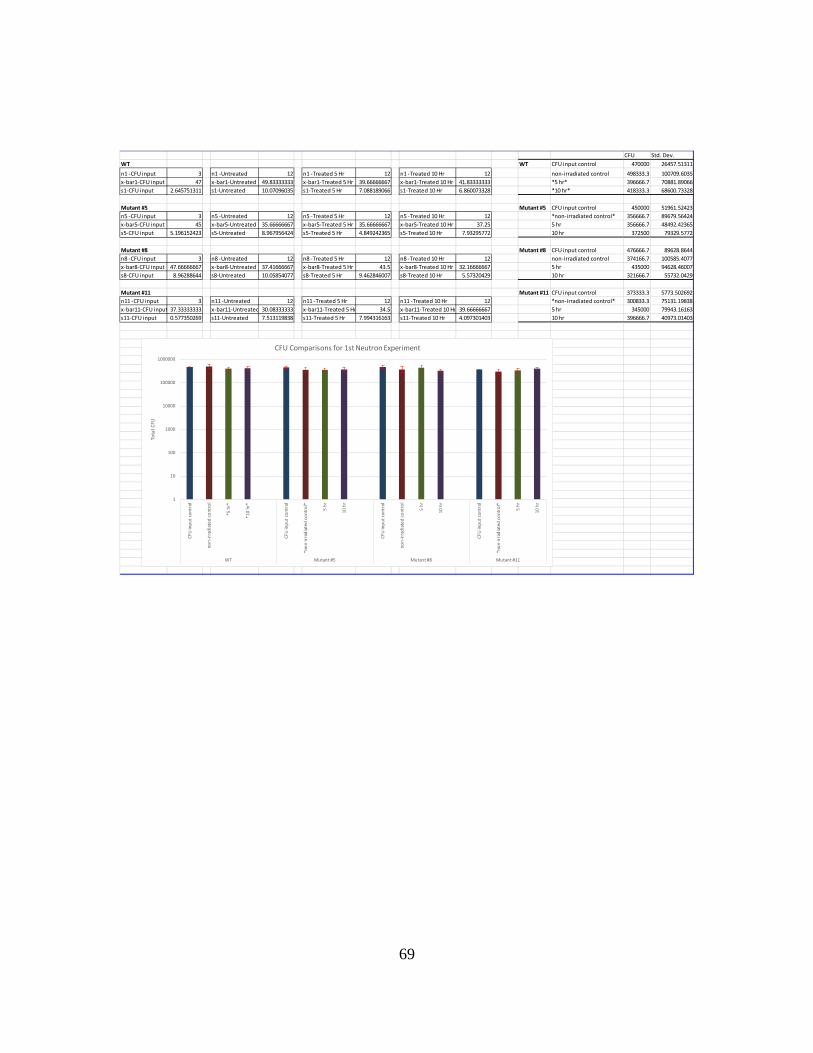
69
CFU Std. Dev.WT WT CFU input control 470000 26457.51311n1 -CFU input 3 n1 -Untreated 12 n1 -Treated 5 Hr 12 n1 -Treated 10 Hr 12 non-irradiated control 498333.3 100709.6035x-bar1-CFU input 47 x-bar1-Untreated 49.83333333 x-bar1-Treated 5 Hr 39.66666667 x-bar1-Treated 10 Hr 41.83333333 *5 hr* 396666.7 70881.89066s1-CFU input 2.645751311 s1-Untreated 10.07096035 s1-Treated 5 Hr 7.088189066 s1-Treated 10 Hr 6.860073328 *10 hr* 418333.3 68600.73328
Mutant #5 Mutant #5 CFU input control 450000 51961.52423n5 -CFU input 3 n5 -Untreated 12 n5 -Treated 5 Hr 12 n5 -Treated 10 Hr 12 *non-irradiated control* 356666.7 89679.56424x-bar5-CFU input 45 x-bar5-Untreated 35.66666667 x-bar5-Treated 5 Hr 35.66666667 x-bar5-Treated 10 Hr 37.25 5 hr 356666.7 48492.42365s5-CFU input 5.196152423 s5-Untreated 8.967956424 s5-Treated 5 Hr 4.849242365 s5-Treated 10 Hr 7.93295772 10 hr 372500 79329.5772
Mutant #8 Mutant #8 CFU input control 476666.7 89628.8644n8 -CFU input 3 n8 -Untreated 12 n8 -Treated 5 Hr 12 n8 -Treated 10 Hr 12 non-irradiated control 374166.7 100585.4077x-bar8-CFU input 47.66666667 x-bar8-Untreated 37.41666667 x-bar8-Treated 5 Hr 43.5 x-bar8-Treated 10 Hr 32.16666667 5 hr 435000 94628.46007s8-CFU input 8.96288644 s8-Untreated 10.05854077 s8-Treated 5 Hr 9.462846007 s8-Treated 10 Hr 5.57320429 10 hr 321666.7 55732.0429
Mutant #11 Mutant #11 CFU input control 373333.3 5773.502692n11 -CFU input 3 n11 -Untreated 12 n11 -Treated 5 Hr 12 n11 -Treated 10 Hr 12 *non-irradiated control* 300833.3 75131.19838x-bar11-CFU input 37.33333333 x-bar11-Untreated 30.08333333 x-bar11-Treated 5 Hr 34.5 x-bar11-Treated 10 Hr 39.66666667 5 hr 345000 79943.16163s11-CFU input 0.577350269 s11-Untreated 7.513119838 s11-Treated 5 Hr 7.994316163 s11-Treated 10 Hr 4.097301403 10 hr 396666.7 40973.01403
1
10
100
1000
10000
100000
1000000
CFU
inpu
t con
trol
non-
irrad
iate
d co
ntro
l
*5 h
r*
*10
hr*
CFU
inpu
t con
trol
*non
-irra
diat
ed co
ntro
l*
5 hr
10 h
r
CFU
inpu
t con
trol
non-
irrad
iate
d co
ntro
l
5 hr
10 h
r
CFU
inpu
t con
trol
*non
-irra
diat
ed co
ntro
l*
5 hr
10 h
r
WT Mutant #5 Mutant #8 Mutant #11
Tota
l CFU
CFU Comparisons for 1st Neutron Experiment
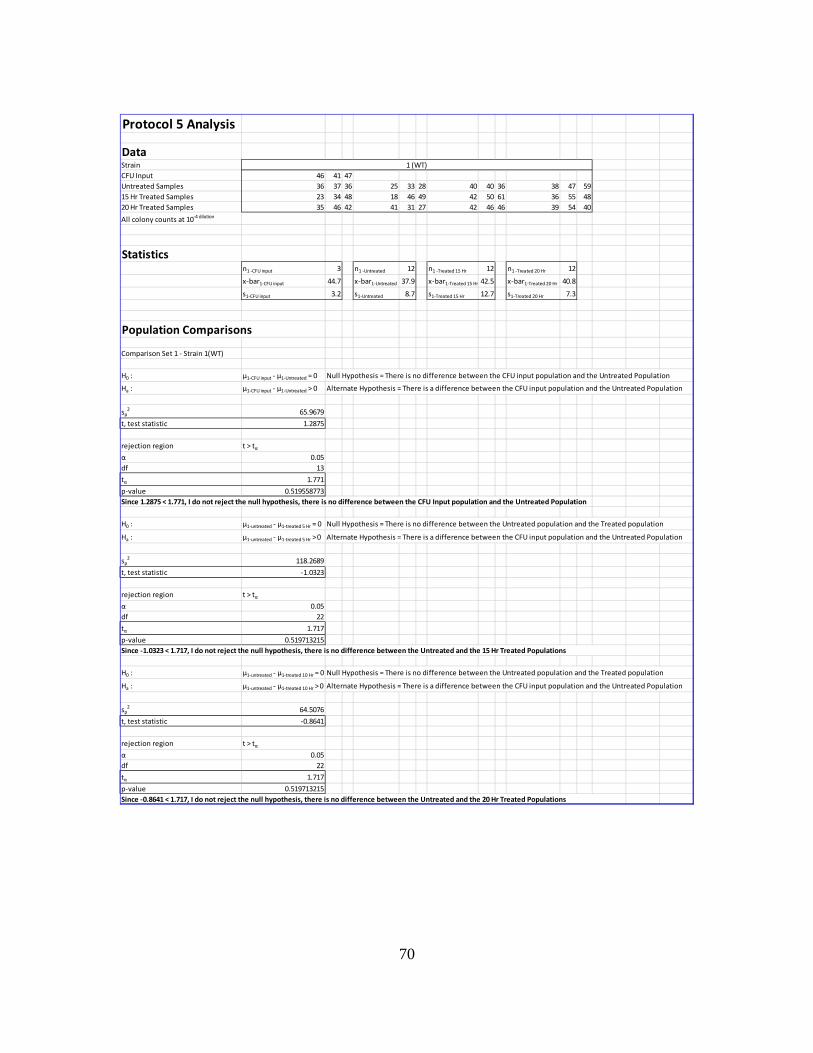
70
Protocol 5 Analysis
DataStrainCFU Input 46 41 47Untreated Samples 36 37 36 25 33 28 40 40 36 38 47 5915 Hr Treated Samples 23 34 48 18 46 49 42 50 61 36 55 4820 Hr Treated Samples 35 46 42 41 31 27 42 46 46 39 54 40All colony counts at 10-4 dilution
Statisticsn1 -CFU input 3 n1 -Untreated 12 n1 -Treated 15 Hr 12 n1 -Treated 20 Hr 12
x-bar1-CFU input 44.7 x-bar1-Untreated 37.9 x-bar1-Treated 15 Hr 42.5 x-bar1-Treated 20 Hr 40.8
s1-CFU input 3.2 s1-Untreated 8.7 s1-Treated 15 Hr 12.7 s1-Treated 20 Hr 7.3
Population Comparisons
Comparison Set 1 - Strain 1(WT)
H0 : µ1-CFU input - µ1-Untreated = 0
Ha : µ1-CFU input - µ1-Untreated > 0
sp2 65.9679
t, test statistic 1.2875
rejection region t > tα
α 0.05df 13tα 1.771p-value 0.519558773
H0 : µ1-untreated - µ1-treated 5 Hr = 0
Ha : µ1-untreated - µ1-treated 5 Hr > 0
sp2 118.2689
t, test statistic -1.0323
rejection region t > tα
α 0.05df 22tα 1.717p-value 0.519713215
H0 : µ1-untreated - µ1-treated 10 Hr = 0
Ha : µ1-untreated - µ1-treated 10 Hr > 0
sp2 64.5076
t, test statistic -0.8641
rejection region t > tα
α 0.05df 22tα 1.717p-value 0.519713215
Alternate Hypothesis = There is a difference between the CFU input population and the Untreated Population
Since -1.0323 < 1.717, I do not reject the null hypothesis, there is no difference between the Untreated and the 15 Hr Treated Populations
Null Hypothesis = There is no difference between the Untreated population and the Treated population
Alternate Hypothesis = There is a difference between the CFU input population and the Untreated Population
Since -0.8641 < 1.717, I do not reject the null hypothesis, there is no difference between the Untreated and the 20 Hr Treated Populations
Null Hypothesis = There is no difference between the Untreated population and the Treated population
1 (WT)
Null Hypothesis = There is no difference between the CFU input population and the Untreated Population
Alternate Hypothesis = There is a difference between the CFU input population and the Untreated Population
Since 1.2875 < 1.771, I do not reject the null hypothesis, there is no difference between the CFU Input population and the Untreated Population
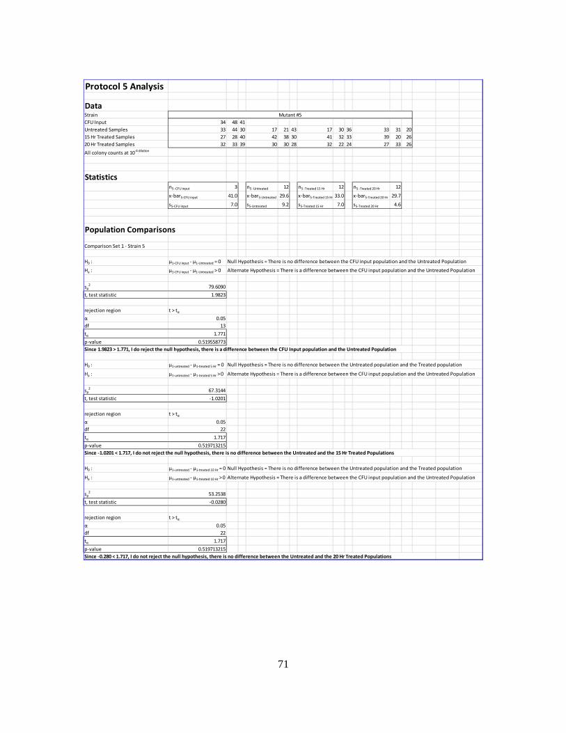
71
Protocol 5 Analysis
DataStrainCFU Input 34 48 41Untreated Samples 33 44 30 17 21 43 17 30 36 33 31 2015 Hr Treated Samples 27 28 40 42 38 30 41 32 33 39 20 2620 Hr Treated Samples 32 33 39 30 30 28 32 22 24 27 33 26All colony counts at 10-4 dilution
Statisticsn5 -CFU input 3 n5 -Untreated 12 n5 -Treated 15 Hr 12 n5 -Treated 20 Hr 12
x-bar5-CFU input 41.0 x-bar5-Untreated 29.6 x-bar5-Treated 15 Hr 33.0 x-bar5-Treated 20 Hr 29.7
s5-CFU input 7.0 s5-Untreated 9.2 s5-Treated 15 Hr 7.0 s5-Treated 20 Hr 4.6
Population Comparisons
Comparison Set 1 - Strain 5
H0 : µ1-CFU input - µ1-Untreated = 0
Ha : µ1-CFU input - µ1-Untreated > 0
sp2 79.6090
t, test statistic 1.9823
rejection region t > tα
α 0.05df 13tα 1.771p-value 0.519558773
H0 : µ1-untreated - µ1-treated 5 Hr = 0
Ha : µ1-untreated - µ1-treated 5 Hr > 0
sp2 67.3144
t, test statistic -1.0201
rejection region t > tα
α 0.05df 22tα 1.717p-value 0.519713215
H0 : µ1-untreated - µ1-treated 10 Hr = 0
Ha : µ1-untreated - µ1-treated 10 Hr > 0
sp2 53.2538
t, test statistic -0.0280
rejection region t > tα
α 0.05df 22tα 1.717p-value 0.519713215
Alternate Hypothesis = There is a difference between the CFU input population and the Untreated Population
Since -1.0201 < 1.717, I do not reject the null hypothesis, there is no difference between the Untreated and the 15 Hr Treated Populations
Null Hypothesis = There is no difference between the Untreated population and the Treated population
Alternate Hypothesis = There is a difference between the CFU input population and the Untreated Population
Since -0.280 < 1.717, I do not reject the null hypothesis, there is no difference between the Untreated and the 20 Hr Treated Populations
Null Hypothesis = There is no difference between the Untreated population and the Treated population
Mutant #5
Null Hypothesis = There is no difference between the CFU input population and the Untreated Population
Alternate Hypothesis = There is a difference between the CFU input population and the Untreated Population
Since 1.9823 > 1.771, I do reject the null hypothesis, there is a difference between the CFU Input population and the Untreated Population

72
Protocol 5 Analysis
DataStrainCFU Input 47 39 46Untreated Samples 22 20 31 20 20 29 30 21 27 31 40 3415 Hr Treated Samples 37 43 23 31 40 54 36 31 27 32 24 2020 Hr Treated Samples 28 36 29 33 26 35 18 18 5 18 30 31All colony counts at 10-4 dilution
Statisticsn8 -CFU input 3 n8 -Untreated 12 n8 -Treated 15 Hr 12 n8 -Treated 20 Hr 12
x-bar8-CFU input 44.0 x-bar8-Untreated 27.1 x-bar8-Treated 15 Hr 33.2 x-bar8-Treated 20 Hr 25.6
s8-CFU input 4.4 s8-Untreated 6.5 s8-Treated 15 Hr 9.6 s8-Treated 20 Hr 9.1
Population Comparisons
Comparison Set 3 - Strain 8
H0 : µ1-CFU input - µ1-Untreated = 0
Ha : µ1-CFU input - µ1-Untreated > 0
sp2 39.1474
t, test statistic 4.1886
rejection region t > tα
α 0.05df 13tα 1.771p-value 0.519558773
H0 : µ1-untreated - µ1-treated 5 Hr = 0
Ha : µ1-untreated - µ1-treated 5 Hr > 0
sp2 67.2992
t, test statistic -1.8164
rejection region t > tα
α 0.05df 22tα 1.717p-value 0.519713215
H0 : µ1-untreated - µ1-treated 10 Hr = 0
Ha : µ1-untreated - µ1-treated 10 Hr > 0
sp2 62.9924
t, test statistic 0.4629
rejection region t > tα
α 0.05df 22tα 1.717p-value 0.519713215
Alternate Hypothesis = There is a difference between the CFU input population and the Untreated Population
Since -1.8164 < 1.717, I do not reject the null hypothesis, there is no difference between the Untreated and the 15 Hr Treated Populations
Null Hypothesis = There is no difference between the Untreated population and the Treated population
Alternate Hypothesis = There is a difference between the CFU input population and the Untreated Population
Since .4629 < 1.717, I do not reject the null hypothesis, there is no difference between the Untreated and the 10 Hr Treated Populations
Null Hypothesis = There is no difference between the Untreated population and the Treated population
Mutant #8
Null Hypothesis = There is no difference between the CFU input population and the Untreated Population
Alternate Hypothesis = There is a difference between the CFU input population and the Untreated Population
Since 4.1886 > 1.771, I do reject the null hypothesis, there is a difference between the CFU Input population and the Untreated Population
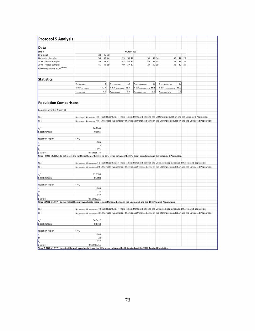
73
Protocol 5 Analysis
DataStrainCFU Input 38 46 38Untreated Samples 50 37 44 33 38 42 56 42 34 52 47 2015 Hr Treated Samples 36 33 37 55 43 34 46 35 43 38 36 3020 Hr Treated Samples 41 45 39 40 37 37 29 50 39 46 30 25All colony counts at 10-4 dilution
Statisticsn11 -CFU input 3 n11 -Untreated 12 n11 -Treated 15 Hr 12 n11 -Treated 20 Hr 12
x-bar11-CFU input 40.7 x-bar11-Untreated 41.3 x-bar11-Treated 15 Hr 38.8 x-bar11-Treated 20 Hr 38.2
s11-CFU input 4.6 s11-Untreated 9.8 s11-Treated 15 Hr 6.9 s11-Treated 20 Hr 7.3
Population Comparisons
Comparison Set 4 - Strain 11
H0 : µ1-CFU input - µ1-Untreated = 0
Ha : µ1-CFU input - µ1-Untreated > 0
sp2 84.2244
t, test statistic -0.0985
rejection region t > tα
α 0.05df 13tα 1.771p-value 0.519558773
H0 : µ1-untreated - µ1-treated 5 Hr = 0
Ha : µ1-untreated - µ1-treated 5 Hr > 0
sp2 71.3598
t, test statistic 0.7008
rejection region t > tα
α 0.05df 22tα 1.717p-value 0.519713215
H0 : µ1-untreated - µ1-treated 10 Hr = 0
Ha : µ1-untreated - µ1-treated 10 Hr > 0
sp2 74.5417
t, test statistic 0.8748
rejection region t > tα
α 0.05df 22tα 1.717p-value 0.519713215
Alternate Hypothesis = There is a difference between the CFU input population and the Untreated Population
Since .07008 < 1.717, I do not reject the null hypothesis, there is no difference between the Untreated and the 15 Hr Treated Populations
Null Hypothesis = There is no difference between the Untreated population and the Treated population
Alternate Hypothesis = There is a difference between the CFU input population and the Untreated Population
Since 0.8748 > 1.717, I do reject the null hypothesis, there is a difference between the Untreated and the 20 Hr Treated Populations
Null Hypothesis = There is no difference between the Untreated population and the Treated population
Mutant #11
Null Hypothesis = There is no difference between the CFU input population and the Untreated Population
Alternate Hypothesis = There is a difference between the CFU input population and the Untreated Population
Since -.0985 < 1.771, I do not reject the null hypothesis, there is no difference between the CFU Input population and the Untreated Population
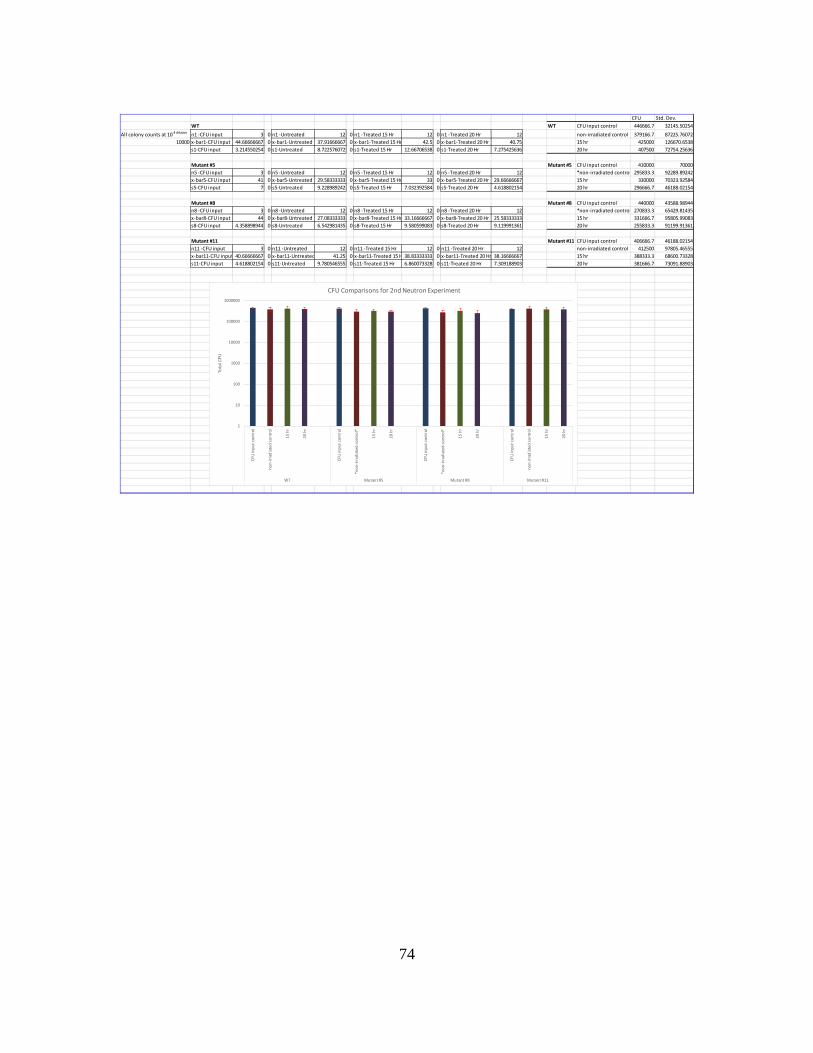
74
CFU Std. Dev.WT WT CFU input control 446666.7 32145.50254
All colony counts at 10-4 dilution n1 -CFU input 3 0 n1 -Untreated 12 0 n1 -Treated 15 Hr 12 0 n1 -Treated 20 Hr 12 non-irradiated control 379166.7 87225.7607210000 x-bar1-CFU input 44.66666667 0 x-bar1-Untreated 37.91666667 0 x-bar1-Treated 15 Hr 42.5 0 x-bar1-Treated 20 Hr 40.75 15 hr 425000 126670.6538
s1-CFU input 3.214550254 0 s1-Untreated 8.722576072 0 s1-Treated 15 Hr 12.66706538 0 s1-Treated 20 Hr 7.275425636 20 hr 407500 72754.25636
Mutant #5 Mutant #5 CFU input control 410000 70000n5 -CFU input 3 0 n5 -Untreated 12 0 n5 -Treated 15 Hr 12 0 n5 -Treated 20 Hr 12 *non-irradiated control 295833.3 92289.89242x-bar5-CFU input 41 0 x-bar5-Untreated 29.58333333 0 x-bar5-Treated 15 Hr 33 0 x-bar5-Treated 20 Hr 29.66666667 15 hr 330000 70323.92584s5-CFU input 7 0 s5-Untreated 9.228989242 0 s5-Treated 15 Hr 7.032392584 0 s5-Treated 20 Hr 4.618802154 20 hr 296666.7 46188.02154
Mutant #8 Mutant #8 CFU input control 440000 43588.98944n8 -CFU input 3 0 n8 -Untreated 12 0 n8 -Treated 15 Hr 12 0 n8 -Treated 20 Hr 12 *non-irradiated control 270833.3 65429.81435x-bar8-CFU input 44 0 x-bar8-Untreated 27.08333333 0 x-bar8-Treated 15 Hr 33.16666667 0 x-bar8-Treated 20 Hr 25.58333333 15 hr 331666.7 95805.99083s8-CFU input 4.358898944 0 s8-Untreated 6.542981435 0 s8-Treated 15 Hr 9.580599083 0 s8-Treated 20 Hr 9.119991361 20 hr 255833.3 91199.91361
Mutant #11 Mutant #11 CFU input control 406666.7 46188.02154n11 -CFU input 3 0 n11 -Untreated 12 0 n11 -Treated 15 Hr 12 0 n11 -Treated 20 Hr 12 non-irradiated control 412500 97805.46555x-bar11-CFU input 40.66666667 0 x-bar11-Untreated 41.25 0 x-bar11-Treated 15 H 38.83333333 0 x-bar11-Treated 20 Hr 38.16666667 15 hr 388333.3 68600.73328s11-CFU input 4.618802154 0 s11-Untreated 9.780546555 0 s11-Treated 15 Hr 6.860073328 0 s11-Treated 20 Hr 7.309188903 20 hr 381666.7 73091.88903
1
10
100
1000
10000
100000
1000000
CFU
inpu
t con
trol
non-
irrad
iate
d co
ntro
l
15 h
r
20 h
r
CFU
inpu
t con
trol
*non
-irra
diat
ed co
ntro
l*
15 h
r
20 h
r
CFU
inpu
t con
trol
*non
-irra
diat
ed co
ntro
l*
15 h
r
20 h
r
CFU
inpu
t con
trol
non-
irrad
iate
d co
ntro
l
15 h
r
20 h
r
WT Mutant #5 Mutant #8 Mutant #11
Tota
l CFU
CFU Comparisons for 2nd Neutron Experiment
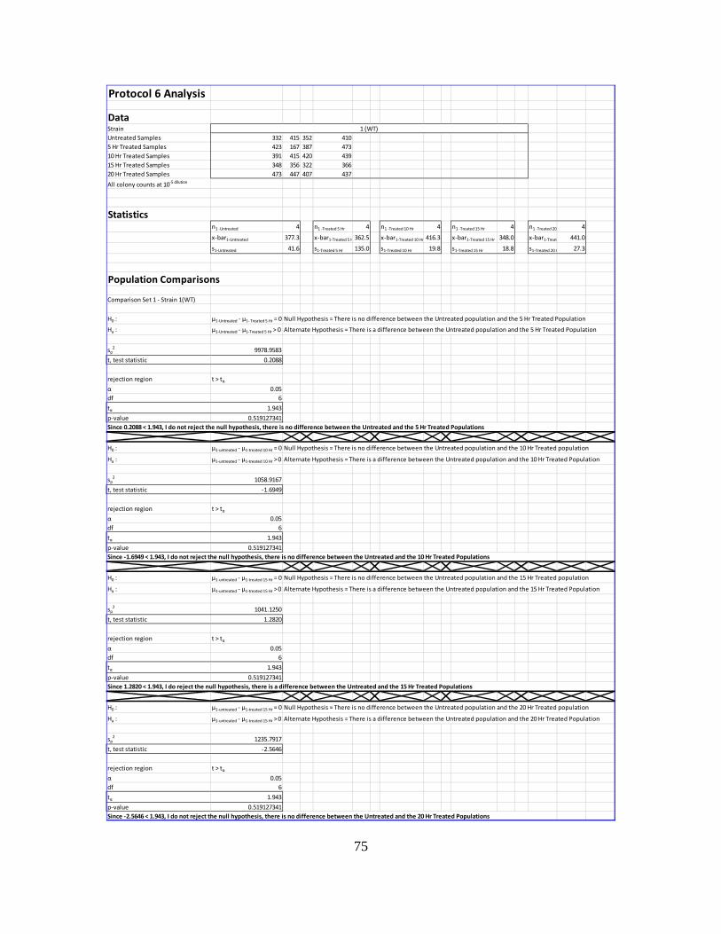
75
Protocol 6 Analysis
DataStrainUntreated Samples 332 415 352 4105 Hr Treated Samples 423 167 387 47310 Hr Treated Samples 391 415 420 43915 Hr Treated Samples 348 356 322 36620 Hr Treated Samples 473 447 407 437All colony counts at 10-5 dilution
Statisticsn1 -Untreated 4 n1 -Treated 5 Hr 4 n1 -Treated 10 Hr 4 n1 -Treated 15 Hr 4 n1 -Treated 20 4
x-bar1-Untreated 377.3 x-bar1-Treated 5 H 362.5 x-bar1-Treated 10 Hr 416.3 x-bar1-Treated 15 Hr 348.0 x-bar1-Treat 441.0
s1-Untreated 41.6 s1-Treated 5 Hr 135.0 s1-Treated 10 Hr 19.8 s1-Treated 15 Hr 18.8 s1-Treated 20 H 27.3
Population Comparisons
Comparison Set 1 - Strain 1(WT)
H0 : µ1-Untreated - µ1- Treated 5 Hr = 0
Ha : µ1-Untreated - µ1-Treated 5 Hr > 0
sp2 9978.9583
t, test statistic 0.2088
rejection region t > tα
α 0.05df 6tα 1.943p-value 0.519127341
H0 : µ1-untreated - µ1-treated 10 Hr = 0
Ha : µ1-untreated - µ1-treated 10 Hr > 0
sp2 1058.9167
t, test statistic -1.6949
rejection region t > tα
α 0.05df 6tα 1.943p-value 0.519127341
H0 : µ1-untreated - µ1-treated 15 Hr = 0
Ha : µ1-untreated - µ1-treated 15 Hr > 0
sp2 1041.1250
t, test statistic 1.2820
rejection region t > tα
α 0.05df 6tα 1.943p-value 0.519127341
H0 : µ1-untreated - µ1-treated 15 Hr = 0
Ha : µ1-untreated - µ1-treated 15 Hr > 0
sp2 1235.7917
t, test statistic -2.5646
rejection region t > tα
α 0.05df 6tα 1.943p-value 0.519127341
Alternate Hypothesis = There is a difference between the Untreated population and the 10 Hr Treated Population
1 (WT)
Null Hypothesis = There is no difference between the Untreated population and the 5 Hr Treated Population
Alternate Hypothesis = There is a difference between the Untreated population and the 5 Hr Treated Population
Since 0.2088 < 1.943, I do not reject the null hypothesis, there is no difference between the Untreated and the 5 Hr Treated Populations
Null Hypothesis = There is no difference between the Untreated population and the 10 Hr Treated population
Since -2.5646 < 1.943, I do not reject the null hypothesis, there is no difference between the Untreated and the 20 Hr Treated Populations
Since -1.6949 < 1.943, I do not reject the null hypothesis, there is no difference between the Untreated and the 10 Hr Treated Populations
Null Hypothesis = There is no difference between the Untreated population and the 15 Hr Treated population
Alternate Hypothesis = There is a difference between the Untreated population and the 15 Hr Treated Population
Since 1.2820 < 1.943, I do reject the null hypothesis, there is a difference between the Untreated and the 15 Hr Treated Populations
Null Hypothesis = There is no difference between the Untreated population and the 20 Hr Treated population
Alternate Hypothesis = There is a difference between the Untreated population and the 20 Hr Treated Population
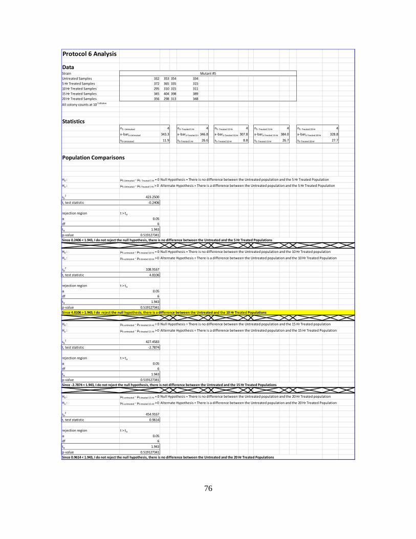
76
Protocol 6 Analysis
DataStrainUntreated Samples 332 353 354 3345 Hr Treated Samples 372 365 335 31510 Hr Treated Samples 295 310 315 31115 Hr Treated Samples 345 404 398 38920 Hr Treated Samples 356 298 313 348All colony counts at 10-5 dilution
Statisticsn5 -Untreated 4 n5 -Treated 5 Hr 4 n5 -Treated 10 Hr 4 n5 -Treated 15 Hr 4 n5 -Treated 20 Hr 4
x-bar5-Untreated 343.3 x-bar5-Treated 5 H 346.8 x-bar5-Treated 10 Hr 307.8 x-bar5-Treated 15 Hr 384.0 x-bar5-Treated 20 Hr 328.8
s5-Untreated 11.9 s5-Treated 5 Hr 26.6 s5-Treated 10 Hr 8.8 s5-Treated 15 Hr 26.7 s5-Treated 20 Hr 27.7
Population Comparisons
H0 : µ5-Untreated - µ5- Treated 5 Hr = 0
Ha : µ5-Untreated - µ5-Treated 5 Hr > 0
sp2 423.2500
t, test statistic -0.2406
rejection region t > tα
α 0.05df 6tα 1.943p-value 0.519127341
H0 : µ5-untreated - µ5-treated 10 Hr = 0
Ha : µ5-untreated - µ5-treated 10 Hr > 0
sp2 108.9167
t, test statistic 4.8106
rejection region t > tα
α 0.05df 6tα 1.943p-value 0.519127341
H0 : µ5-untreated - µ5-treated 15 Hr = 0
Ha : µ5-untreated - µ5-treated 15 Hr > 0
sp2 427.4583
t, test statistic -2.7874
rejection region t > tα
α 0.05df 6tα 1.943p-value 0.519127341
H0 : µ5-untreated - µ5-treated 15 Hr = 0
Ha : µ5-untreated - µ5-treated 15 Hr > 0
sp2 454.9167
t, test statistic 0.9614
rejection region t > tα
α 0.05df 6tα 1.943p-value 0.519127341
Alternate Hypothesis = There is a difference between the Untreated population and the 10 Hr Treated Population
Mutant #5
Null Hypothesis = There is no difference between the Untreated population and the 5 Hr Treated Population
Alternate Hypothesis = There is a difference between the Untreated population and the 5 Hr Treated Population
Since 0.2406 < 1.943, I do not reject the null hypothesis, there is no difference between the Untreated and the 5 Hr Treated Populations
Null Hypothesis = There is no difference between the Untreated population and the 10 Hr Treated population
Since 0.9614 < 1.943, I do not reject the null hypothesis, there is no difference between the Untreated and the 20 Hr Treated Populations
Since 4.8106 > 1.943, I do reject the null hypothesis, there is a difference between the Untreated and the 10 Hr Treated Populations
Null Hypothesis = There is no difference between the Untreated population and the 15 Hr Treated population
Alternate Hypothesis = There is a difference between the Untreated population and the 15 Hr Treated Population
Since -2.7874 < 1.943, I do not reject the null hypothesis, there is not difference between the Untreated and the 15 Hr Treated Populations
Null Hypothesis = There is no difference between the Untreated population and the 20 Hr Treated population
Alternate Hypothesis = There is a difference between the Untreated population and the 20 Hr Treated Population
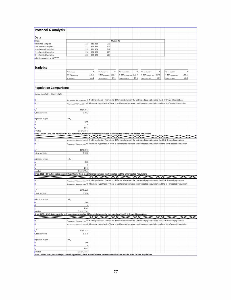
77
Protocol 6 Analysis
DataStrainUntreated Samples 333 311 382 2765 Hr Treated Samples 317 364 345 30710 Hr Treated Samples 333 331 304 31715 Hr Treated Samples 316 329 300 28520 Hr Treated Samples 233 332 320 269All colony counts at 10-5 dilution
Statisticsn8 -Untreated 4 n8 -Treated 5 Hr 4 n8 -Treated 10 Hr 4 n8 -Treated 15 Hr 4 n8 -Treated 20 Hr 4
x-bar8-Untreated 325.5 x-bar8-Treated 5 H 333.3 x-bar8-Treated 10 Hr 321.3 x-bar8-Treated 15 Hr 307.5 x-bar8-Treated 20 Hr 288.5
s8-Untreated 44.4 s8-Treated 5 Hr 26.1 s8-Treated 10 Hr 13.5 s8-Treated 15 Hr 19.1 s8-Treated 20 Hr 46.0
Population Comparisons
Comparison Set 1 - Strain 1(WT)
H0 : µ8-Untreated - µ8- Treated 5 Hr = 0
Ha : µ8-Untreated - µ8-Treated 5 Hr > 0
sp2 1324.2917
t, test statistic -0.3012
rejection region t > tα
α 0.05df 6tα 1.943p-value 0.519127341
H0 : µ8-untreated - µ8-treated 10 Hr = 0
Ha : µ8-untreated - µ8-treated 10 Hr > 0
sp2 1076.2917
t, test statistic 0.1832
rejection region t > tα
α 0.05df 6tα 1.943p-value 0.519127341
H0 : µ8-untreated - µ8-treated 15 Hr = 0
Ha : µ8-untreated - µ8-treated 15 Hr > 0
sp2 1167.6667
t, test statistic 0.7450
rejection region t > tα
α 0.05df 6tα 1.943p-value 0.519127341
H0 : µ8-untreated - µ8-treated 15 Hr = 0
Ha : µ8-untreated - µ8-treated 15 Hr > 0
sp2 2042.3333
t, test statistic 1.1579
rejection region t > tα
α 0.05df 6tα 1.943p-value 0.519127341
Alternate Hypothesis = There is a difference between the Untreated population and the 10 Hr Treated Population
Mutant #8
Null Hypothesis = There is no difference between the Untreated population and the 5 Hr Treated Population
Alternate Hypothesis = There is a difference between the Untreated population and the 5 Hr Treated Population
Since -.3012 < 1.943, I do not reject the null hypothesis, there is no difference between the Untreated and the 5 Hr Treated Populations
Null Hypothesis = There is no difference between the Untreated population and the 10 Hr Treated population
Since 1.1579 < 1.943, I do not reject the null hypothesis, there is no difference between the Untreated and the 20 Hr Treated Populations
Since .1832 < 1.943, I do reject the null hypothesis, there is a difference between the Untreated and the 10 Hr Treated Populations
Null Hypothesis = There is no difference between the Untreated population and the 15 Hr Treated population
Alternate Hypothesis = There is a difference between the Untreated population and the 15 Hr Treated Population
Since .7450 < 1.943, I do reject the null hypothesis, there is a difference between the Untreated and the 15 Hr Treated Populations
Null Hypothesis = There is no difference between the Untreated population and the 20 Hr Treated population
Alternate Hypothesis = There is a difference between the Untreated population and the 20 Hr Treated Population
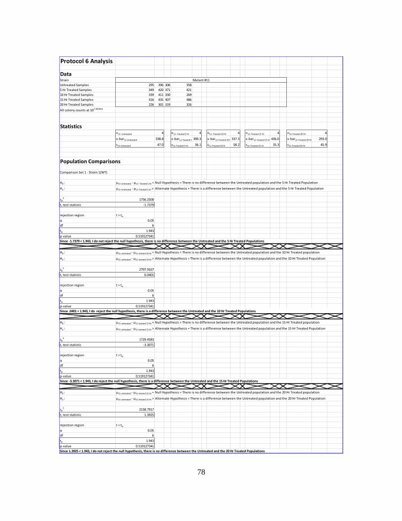
78
Protocol 6 Analysis
DataStrainUntreated Samples 295 396 306 3585 Hr Treated Samples 349 420 371 42110 Hr Treated Samples 339 411 330 26915 Hr Treated Samples 416 435 407 48620 Hr Treated Samples 226 301 319 326All colony counts at 10-5 dilution
Statisticsn11 -Untreated 4 n11 -Treated 5 Hr 4 n11 -Treated 10 Hr 4 n11-Treated 15 Hr 4 n11-Treated 20 Hr 4
x-bar11-Untreated 338.8 x-bar11-Treated 5 390.3 x-bar11-Treated 10 H 337.3 x-bar11-Treated 15 Hr 436.0 x-bar11-Treated 20 Hr 293.0
s11-Untreated 47.0 s11-Treated 5 Hr 36.1 s11-Treated 10 Hr 58.2 s11-Treated 15 Hr 35.3 s11-Treated 20 Hr 45.9
Population Comparisons
Comparison Set 1 - Strain 1(WT)
H0 : µ11-Untreated - µ11- Treated 5 Hr =
Ha : µ11-Untreated - µ11-Treated 5 Hr > 0
sp2 1756.2500
t, test statistic -1.7379
rejection region t > tα
α 0.05df 6tα 1.943p-value 0.519127341
H0 : µ11-untreated - µ11-treated 10 Hr =
Ha : µ11-untreated - µ11-treated 10 Hr >
sp2 2797.9167
t, test statistic 0.0401
rejection region t > tα
α 0.05df 6tα 1.943p-value 0.519127341
H0 : µ11-untreated - µ11-treated 15 Hr =
Ha : µ11-untreated - µ11-treated 15 Hr >
sp2 1729.4583
t, test statistic -3.3071
rejection region t > tα
α 0.05df 6tα 1.943p-value 0.519127341
H0 : µ11-untreated - µ11-treated 15 Hr =
Ha : µ11-untreated - µ11-treated 15 Hr >
sp2 2158.7917
t, test statistic 1.3925
rejection region t > tα
α 0.05df 6tα 1.943p-value 0.519127341
Alternate Hypothesis = There is a difference between the Untreated population and the 10 Hr Treated Population
Mutant #11
Null Hypothesis = There is no difference between the Untreated population and the 5 Hr Treated Population
Alternate Hypothesis = There is a difference between the Untreated population and the 5 Hr Treated Population
Since -1.7379 < 1.943, I do not reject the null hypothesis, there is no difference between the Untreated and the 5 Hr Treated Populations
Null Hypothesis = There is no difference between the Untreated population and the 10 Hr Treated population
Since 1.3925 < 1.943, I do not reject the null hypothesis, there is no difference between the Untreated and the 20 Hr Treated Populations
Since .0401 < 1.943, I do reject the null hypothesis, there is a difference between the Untreated and the 10 Hr Treated Populations
Null Hypothesis = There is no difference between the Untreated population and the 15 Hr Treated population
Alternate Hypothesis = There is a difference between the Untreated population and the 15 Hr Treated Population
Since -3.3071 < 1.943, I do reject the null hypothesis, there is a difference between the Untreated and the 15 Hr Treated Populations
Null Hypothesis = There is no difference between the Untreated population and the 20 Hr Treated population
Alternate Hypothesis = There is a difference between the Untreated population and the 20 Hr Treated Population

79
Protocol 6 Analysis
DataStrainUntreated Samples 15 23 11 16 24 11 13 13 colony counts at 10-2 dilution
5 Hr Treated Samples 2 4 3 3 5 7 4 4 colony counts at 10-2 dilution
10 Hr Treated Samples 2 5 3 4 8 4 2 4 colony counts at 10-2 dilution
15 Hr Treated Samples 1 1 7 3 2 1 3 2 colony counts at 10-2 dilution
20 Hr Treated Samples 8 5 10 12 7 3 17 9 colony counts at 10-2 dilution
StatisticsnEC -Untreated 8 nEC -Treated 5 Hr 8 nEC -Treated 10 Hr 8 nEC-Treated 15 Hr 8 nEC-Treated 20 Hr 8
x-barEC-Untreated 15.8 x-barEC-Treated 5 4.0 x-barEC-Treated 10 H 4.0 x-barEC-Treated 15 Hr 2.5 x-barEC-Treated 20 Hr 8.9
sEC-Untreated 5.1 sEC-Treated 5 Hr 1.5 sEC-Treated 10 Hr 1.9 sEC-Treated 15 Hr 2.0 sEC-Treated 20 Hr 4.3
Population Comparisons
Comparison Set 1 - Strain 1(WT)
H0 : µEC-Untreated - µEC- Treated 5 Hr =
Ha : µEC-Untreated - µEC-Treated 5 Hr > 0
sp2 14.1071
t, test statistic 6.2567
rejection region t > tα
α 0.05df 14tα 1.761p-value 0.519585629
H0 : µEC-untreated - µEC-treated 10 Hr =
Ha : µEC-untreated - µEC-treated 10 Hr >
sp2 14.8214
t, test statistic 6.1041
rejection region t > tα
α 0.05df 14tα 1.761p-value 0.519585629
H0 : µEC-untreated - µEC-treated 15 Hr =
Ha : µEC-untreated - µEC-treated 15 Hr >
sp2 14.9643
t, test statistic 6.8504
rejection region t > tα
α 0.05df 14tα 1.761p-value 0.519585629
H0 : µEC-untreated - µ-ECtreated 15 Hr =
Ha : µEC-untreated - µEC-treated 15 Hr >
sp2 22.3125
t, test statistic 2.9109
rejection region t > tα
α 0.05df 14tα 1.761p-value 0.519585629
Alternate Hypothesis = There is a difference between the Untreated population and the 10 Hr Treated Population
EC
Null Hypothesis = There is no difference between the Untreated population and the 5 Hr Treated Population
Alternate Hypothesis = There is a difference between the Untreated population and the 5 Hr Treated Population
Since 6.2567 > 1.761, I do reject the null hypothesis, there is a difference between the Untreated and the 5 Hr Treated Populations
Null Hypothesis = There is no difference between the Untreated population and the 10 Hr Treated population
Since 2.9109 > 1.761 I do reject the null hypothesis, there is a difference between the Untreated and the 20 Hr Treated Populations
Since 6.1041 > 1.761, I do reject the null hypothesis, there is a difference between the Untreated and the 10 Hr Treated Populations
Null Hypothesis = There is no difference between the Untreated population and the 15 Hr Treated population
Alternate Hypothesis = There is a difference between the Untreated population and the 15 Hr Treated Population
Since 6.8504 > 1.761, I do reject the null hypothesis, there is a difference between the Untreated and the 15 Hr Treated Populations
Null Hypothesis = There is no difference between the Untreated population and the 20 Hr Treated population
Alternate Hypothesis = There is a difference between the Untreated population and the 20 Hr Treated Population
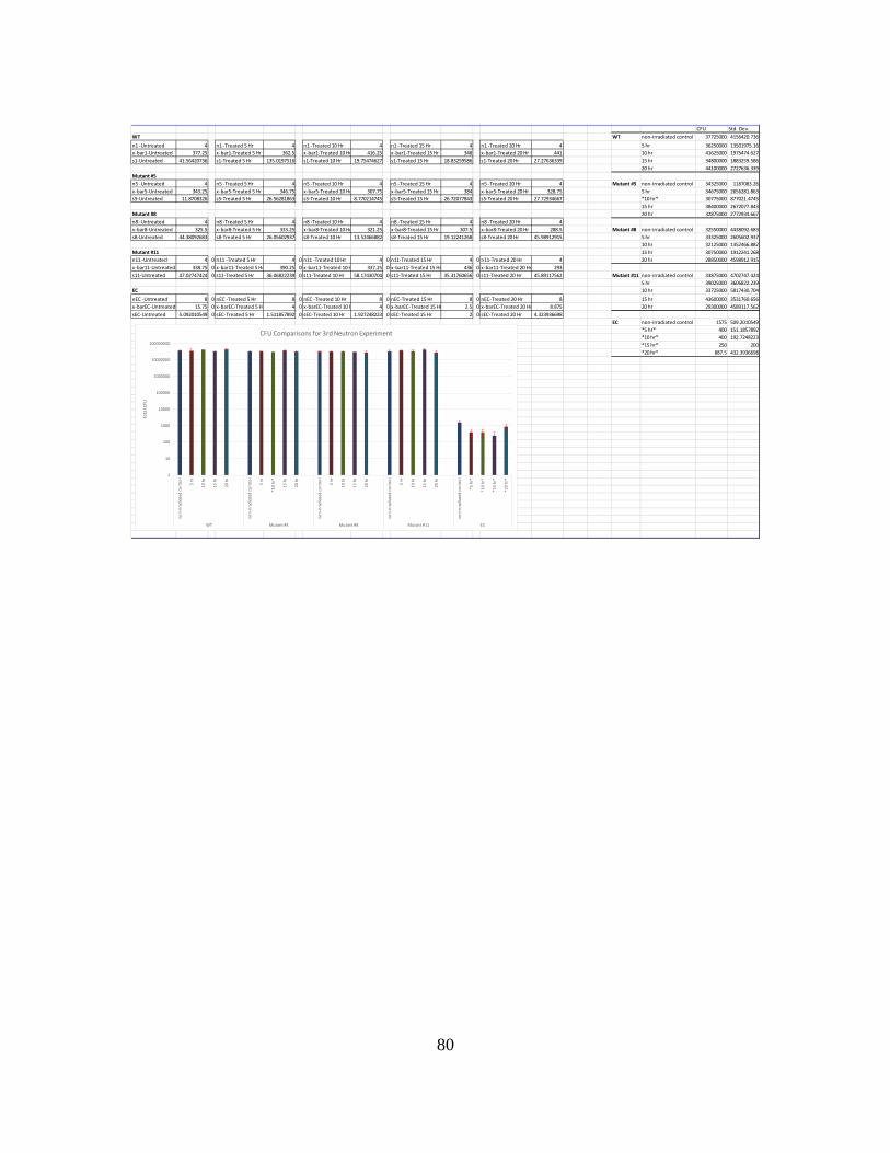
80
CFU Std. Dev.WT WT non-irradiated control 37725000 4156420.736n1 -Untreated 4 n1 -Treated 5 Hr 4 n1 -Treated 10 Hr 4 n1 -Treated 15 Hr 4 n1 -Treated 20 Hr 4 5 hr 36250000 13501975.16x-bar1-Untreated 377.25 x-bar1-Treated 5 Hr 362.5 x-bar1-Treated 10 Hr 416.25 x-bar1-Treated 15 Hr 348 x-bar1-Treated 20 Hr 441 10 hr 41625000 1975474.627s1-Untreated 41.56420736 s1-Treated 5 Hr 135.0197516 s1-Treated 10 Hr 19.75474627 s1-Treated 15 Hr 18.83259586 s1-Treated 20 Hr 27.27636339 15 hr 34800000 1883259.586
20 hr 44100000 2727636.339Mutant #5n5 -Untreated 4 n5 -Treated 5 Hr 4 n5 -Treated 10 Hr 4 n5 -Treated 15 Hr 4 n5 -Treated 20 Hr 4 Mutant #5 non-irradiated control 34325000 1187083.26x-bar5-Untreated 343.25 x-bar5-Treated 5 Hr 346.75 x-bar5-Treated 10 Hr 307.75 x-bar5-Treated 15 Hr 384 x-bar5-Treated 20 Hr 328.75 5 hr 34675000 2656281.863s5-Untreated 11.8708326 s5-Treated 5 Hr 26.56281863 s5-Treated 10 Hr 8.770214745 s5-Treated 15 Hr 26.72077843 s5-Treated 20 Hr 27.72934667 *10 hr* 30775000 877021.4745
15 hr 38400000 2672077.843Mutant #8 20 hr 32875000 2772934.667n8 -Untreated 4 n8 -Treated 5 Hr 4 n8 -Treated 10 Hr 4 n8 -Treated 15 Hr 4 n8 -Treated 20 Hr 4x-bar8-Untreated 325.5 x-bar8-Treated 5 Hr 333.25 x-bar8-Treated 10 Hr 321.25 x-bar8-Treated 15 Hr 307.5 x-bar8-Treated 20 Hr 288.5 Mutant #8 non-irradiated control 32550000 4438092.683s8-Untreated 44.38092683 s8-Treated 5 Hr 26.05602937 s8-Treated 10 Hr 13.52466882 s8-Treated 15 Hr 19.12241268 s8-Treated 20 Hr 45.98912915 5 hr 33325000 2605602.937
10 hr 32125000 1352466.882Mutant #11 15 hr 30750000 1912241.268n11 -Untreated 4 0 n11 -Treated 5 Hr 4 0 n11 -Treated 10 Hr 4 0 n11-Treated 15 Hr 4 0 n11-Treated 20 Hr 4 20 hr 28850000 4598912.915x-bar11-Untreated 338.75 0 x-bar11-Treated 5 Hr 390.25 0 x-bar11-Treated 10 H 337.25 0 x-bar11-Treated 15 Hr 436 0 x-bar11-Treated 20 Hr 293s11-Untreated 47.02747424 0 s11-Treated 5 Hr 36.06822239 0 s11-Treated 10 Hr 58.17430704 0 s11-Treated 15 Hr 35.31760656 0 s11-Treated 20 Hr 45.89117562 Mutant #11 non-irradiated control 33875000 4702747.424
5 hr 39025000 3606822.239EC 10 hr 33725000 5817430.704nEC -Untreated 8 0 nEC -Treated 5 Hr 8 0 nEC -Treated 10 Hr 8 0 nEC-Treated 15 Hr 8 0 nEC-Treated 20 Hr 8 15 hr 43600000 3531760.656x-barEC-Untreated 15.75 0 x-barEC-Treated 5 Hr 4 0 x-barEC-Treated 10 H 4 0 x-barEC-Treated 15 Hr 2.5 0 x-barEC-Treated 20 Hr 8.875 20 hr 29300000 4589117.562sEC-Untreated 5.092010549 0 sEC-Treated 5 Hr 1.511857892 0 sEC-Treated 10 Hr 1.927248223 0 sEC-Treated 15 Hr 2 0 sEC-Treated 20 Hr 4.323936698
EC non-irradiated control 1575 509.2010549*5 hr* 400 151.1857892*10 hr* 400 192.7248223*15 hr* 250 200*20 hr* 887.5 432.3936698
1
10
100
1000
10000
100000
1000000
10000000
100000000
non-
irrad
iate
d co
ntro
l
5 hr
10 h
r
15 h
r
20 h
r
non-
irrad
iate
d co
ntro
l
5 hr
*10
hr*
15 h
r
20 h
r
non-
irrad
iate
d co
ntro
l
5 hr
10 h
r
15 h
r
20 h
r
non-
irrad
iate
d co
ntro
l
5 hr
10 h
r
15 h
r
20 h
r
non-
irrad
iate
d co
ntro
l
*5 h
r*
*10
hr*
*15
hr*
*20
hr*
WT Mutant #5 Mutant #8 Mutant #11 EC
Tota
l CFU
CFU Comparisons for 3rd Neutron Experiment
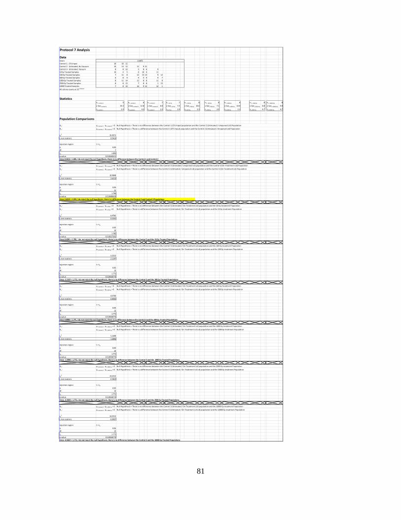
81
Protocol 7 Analysis
DataStrainControl 1 - CFU Input 16 16 11Control 2 - Untreated, No Vacuum 10 13 12 12 9 21Control 3 - Untreated. Vacuum 8 8 12 5 8 6 910 Gy Treated Samples 10 4 5 6 10 6 11100 Gy Treated Samples 7 11 8 12 13 13 9 12500 Gy Treated Samples 6 8 9 4 5 9 9 71000 Gy Treated Samples 8 11 14 12 8 8 11 82500 Gy Treated Samples 8 8 15 7 8 8 1 1510000 Treated Samples 7 8 14 16 9 12 12 1All colony counts at 10-5 dilution
Statisticsn1 -control 1 3 n1 -control 2 6 n1 -control 3 7 n1 -10 Gy 7 n1 -100 Gy 8 n1 - 500 Gy 8 n1 -1000 Gy 8 n1 - 2500 Gy 8 n1 -10000 Gy 8
x-bar1-control 1 14.3 x-bar1-control 2 12.8 x-bar1-control 3 8.0 x-bar1-10 Gy 7.4 x-bar1-100 Gy 10.6 x-bar1-500 Gy 7.1 x-bar1-1000 Gy 10.0 x-bar1-2500 Gy 8.8 x-bar1-10000 Gy 9.9
s1-control 1 2.9 s1-control 2 4.3 s1-control 3 2.2 s1-10 Gy 2.8 s1-100 Gy 2.3 s1-500 Gy 2.0 s1-1000 Gy 2.3 s1-2500 Gy 4.7 s1-10000 Gy 4.7
Population Comparisons
H0 : µ1-Control 1 - µ1-Control 2 = 0
Ha : µ1-Control 1 - µ1-Control 2 > 0
sp2 15.3571
t, test statistic 0.5413
rejection region t > tα
α 0.05df 7tα 1.895p-value 0.519240411
H0 : µ1-Control 2 - µ1-Control 3 = 0
Ha : µ1-Control 2 - µ1-Control 3 > 0
sp2 10.9848
t, test statistic 2.6212
rejection region t > tα
α 0.05df 11tα 1.796p-value 0.519490629
H0 : µ1-Control 3 - µ1-10 Gy = 0
Ha : µ1-Control 3 - µ1-10 Gy > 0
sp2 6.4762
t, test statistic 0.4201
rejection region t > tα
α 0.05df 12tα 1.782p-value 0.519527501
H0 : µ1-Control 3 - µ1-100 Gy = 0
Ha : µ1-Control 3 - µ1-100 Gy > 0
sp2 5.2212
t, test statistic -2.2197
rejection region t > tα
α 0.05df 13tα 1.771p-value 0.519558773
H0 : µ1-Control 3 - µ1-500 Gy = 0
Ha : µ1-Control 3 - µ1-500 Gy > 0
sp2 4.3750
t, test statistic 0.8083
rejection region t > tα
α 0.05df 13tα 1.771p-value 0.519558773
H0 : µ1-Control 3 - µ1-1000 Gy = 0
Ha : µ1-Control 3 - µ1-1000 Gy > 0
sp2 5.2308
t, test statistic -1.6896
rejection region t > tα
α 0.05df 13tα 1.771p-value 0.519558773
H0 : µ1-Control 3 - µ1-1000 Gy = 0
Ha : µ1-Control 3 - µ1-1000 Gy > 0
sp2 14.2212
t, test statistic -0.3843
rejection region t > tα
α 0.05df 13tα 1.771p-value 0.519558773
H0 : µ1-Control 3 - µ1-1000 Gy = 0
Ha : µ1-Control 3 - µ1-1000 Gy > 0
sp2 14.2212
t, test statistic -0.9607
rejection region t > tα
α 0.05df 13tα 1.771p-value 0.519558773
1 (WT)
Since 0.5413 < 1.895, I do not reject the null hypothesis, there is no difference between the Control 1 and Control 2
Since -2.2197 < 1.771, I do not reject the null hypothesis, there is no difference between the Control 3 and the 100 Gy Treated Populations
Since 2.6212 > 1.943, I do reject the null hypothesis, there is s difference between the Control 2 and Control 3 Populations
Since 0.4201 < 1.782, I do not reject the null hypothesis, there is no difference between the Control 3 and the 10 Gy Treated Populations
Null Hypothesis = There is no difference between the Control 1 (CFU Input) population and the Control 2 (Untreated / Unopened Lid) Population
Null Hypothesis = There is a difference between the Control 1 (CFU Input) population and the Control 2 (Untreated / Unopened Lid) Population
Null Hypothesis = There is no difference between the Control 2 (Untreated / Unopened Lid) population and the Control 3 (On Treatment Lid) Population
Null Hypothesis = There is a difference between the Control 2 (Untreated / Unopened Lid) population and the Control 3 (On Treatment Lid) Population
Null Hypothesis = There is no difference between the Control 3 (Untreated / On Treatment Lid) population and the 10 Gy treatment Population
Null Hypothesis = There is a difference between the Control 3 (Untreated / On Treatment Lid Lid) population and the 10 Gy treatment Population
Null Hypothesis = There is no difference between the Control 3 (Untreated / On Treatment Lid) population and the 100 Gy treatment Population
Null Hypothesis = There is a difference between the Control 3 (Untreated / On Treatment Lid Lid) population and the 100 Gy treatment Population
Since -0.9607 < 1.771, I do not reject the null hypothesis, there is no difference between the Control 3 and the 10000 Gy Treated Populations
Since 0.8083 < 1.771, I do not reject the null hypothesis, there is no difference between the Control 3 and the 500 Gy Treated Populations
Since -1.5896 < 1.771, I do not reject the null hypothesis, there is no difference between the Control 3 and the 1000 Gy Treated Populations
Since -0.3843 < 1.771, I do not reject the null hypothesis, there is no difference between the Control 3 and the 2500 Gy Treated Populations
Null Hypothesis = There is no difference between the Control 3 (Untreated / On Treatment Lid) population and the 500 Gy treatment Population
Null Hypothesis = There is a difference between the Control 3 (Untreated / On Treatment Lid Lid) population and the 500 Gy treatment Population
Null Hypothesis = There is no difference between the Control 3 (Untreated / On Treatment Lid) population and the 1000 Gy treatment Population
Null Hypothesis = There is a difference between the Control 3 (Untreated / On Treatment Lid Lid) population and the 1000 Gy treatment Population
Null Hypothesis = There is no difference between the Control 3 (Untreated / On Treatment Lid) population and the 2500 Gy treatment Population
Null Hypothesis = There is a difference between the Control 3 (Untreated / On Treatment Lid Lid) population and the 2500 Gy treatment Population
Null Hypothesis = There is no difference between the Control 3 (Untreated / On Treatment Lid) population and the 10000 Gy treatment Population
Null Hypothesis = There is a difference between the Control 3 (Untreated / On Treatment Lid Lid) population and the 10000 Gy treatment Population
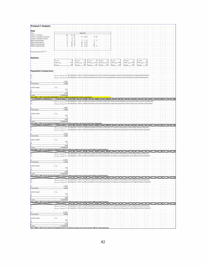
82
Protocol 7 Analysis
DataStrainControl 1 - CFU Input 18 11 12Control 2 - Untreated, No Vacuum 4 7 11 11 10 10 8 10Control 3 - Untreated. Vacuum 7 8 5100 Gy Treated Samples 3 3 8 5 7 9 7 7500 Gy Treated Samples 8 10 8 16 11 16 51000 Gy Treated Samples 9 14 10 13 8 8 102500 Gy Treated Samples 4 10 7 12 8 10 21 6
All colony counts at 10-5 dilution
Statisticsn5 -control 1 3 n5 -control 2 8 n5 -control 3 3 n5 -100 Gy 8 n5- 500 Gy 7 n5 -1000 Gy 7 n5 - 2500 Gy 8
x-bar5-control 1 13.7 x-bar5-control 2 8.9 x-bar5-control 3 6.7 x-bar5-100 Gy 6.1 x-bar5-500 Gy 10.6 x-bar5-1000 Gy 10.3 x-bar5-2500 Gy 9.8
s5-control 1 3.8 s5-control 2 2.4 s5-control 3 1.5 s5-100 Gy 2.2 s5-500 Gy 4.2 s5-1000 Gy 2.4 s5-2500 Gy 5.2
Population Comparisons
H0 : µ5-Control 1 - µ5-Control 2 = 0
Ha : µ5-Control 1 - µ5-Control 2 > 0
sp2 7.7269
t, test statistic 2.5462
rejection region t > tα
α 0.05df 9tα 1.833p-value 0.519392768
H0 : µ5-Control 2 - µ5-Control 3 = 0
Ha : µ5-Control 2 - µ5-Control 3 > 0
sp2 5.0602
t, test statistic 1.4501
rejection region t > tα
α 0.05df 9tα 1.833p-value 0.519392768
H0 : µ5-Control 3 - µ5-100 Gy = 0
Ha : µ5-Control 3 - µ5-100 Gy > 0
sp2 4.3935
t, test statistic 0.3817
rejection region t > tα
α 0.05df 9tα 1.833p-value 0.519392768
H0 : µ5-Control 3 - µ5-500 Gy = 0
Ha : µ5-Control 3 - µ5-500 Gy > 0
sp2 13.5476
t, test statistic -1.5373
rejection region t > tα
α 0.05df 8tα 1.860p-value 0.519325892
H0 : µ5-Control 3 - µ5-1000 Gy = 0
Ha : µ5-Control 3 - µ5-1000 Gy > 0
sp2 4.7619
t, test statistic -2.4033
rejection region t > tα
α 0.05df 8tα 1.860p-value 0.519325892
H0 : µ5-Control 3 - µ5-2500 Gy = 0
Ha : µ5-Control 3 - µ5-2500 Gy > 0
sp2 21.5741
t, test statistic -0.9805
rejection region t > tα
α 0.05df 9tα 1.833p-value 0.519392768
Null Hypothesis = There is a difference between the Control 2 (Untreated / Unopened Lid) population and the Control 3 (On Treatment Lid) Population
Since 1.4501 < 1.833, I do not reject the null hypothesis, there is no difference between the Control 2 and Control 3 Populations
Since -1.5373 < 1.860, I do not reject the null hypothesis, there is no difference between the Control 3 and the 500 Gy Treated Populations
Null Hypothesis = There is no difference between the Control 3 (Untreated / On Treatment Lid) population and the 1000 Gy treatment Population
Null Hypothesis = There is a difference between the Control 3 (Untreated / On Treatment Lid Lid) population and the 1000 Gy treatment Population
Mutant #5
Null Hypothesis = There is no difference between the Control 1 (CFU Input) population and the Control 2 (Untreated / Unopened Lid) Population
Null Hypothesis = There is a difference between the Control 1 (CFU Input) population and the Control 2 (Untreated / Unopened Lid) Population
Since 2.5462 > 1.833, I do reject the null hypothesis, there is a difference between the Control 1 and Control 2
Null Hypothesis = There is no difference between the Control 2 (Untreated / Unopened Lid) population and the Control 3 (On Treatment Lid) Population
Since -0.9805 < 1.833, I do not reject the null hypothesis, there is no difference between the Control 3 and the 2500 Gy Treated Populations
Null Hypothesis = There is no difference between the Control 3 (Untreated / On Treatment Lid) population and the 100 Gy treatment Population
Null Hypothesis = There is a difference between the Control 3 (Untreated / On Treatment Lid Lid) population and the 100 Gy treatment Population
Since 0.3817 < 1.833, I do not reject the null hypothesis, there is no difference between the Control 3 and the 100 Gy Treated Populations
Null Hypothesis = There is no difference between the Control 3 (Untreated / On Treatment Lid) population and the 500 Gy treatment Population
Null Hypothesis = There is a difference between the Control 3 (Untreated / On Treatment Lid Lid) population and the 500 Gy treatment Population
Since -2.4033 < 1.860, I do not reject the null hypothesis, there is no difference between the Control 3 and the 1000 Gy Treated Populations
Null Hypothesis = There is no difference between the Control 3 (Untreated / On Treatment Lid) population and the 2500 Gy treatment Population
Null Hypothesis = There is a difference between the Control 3 (Untreated / On Treatment Lid Lid) population and the 2500 Gy treatment Population
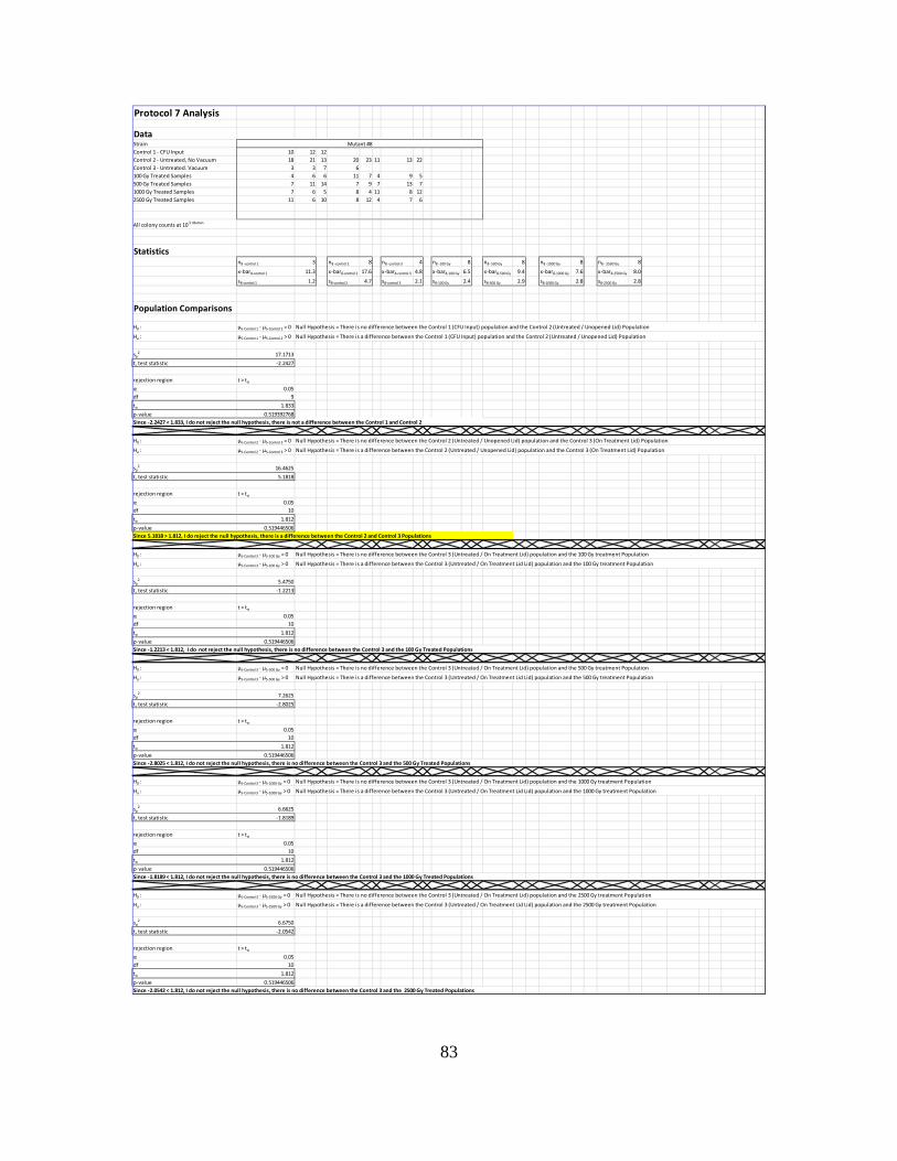
83
Protocol 7 Analysis
DataStrainControl 1 - CFU Input 10 12 12Control 2 - Untreated, No Vacuum 18 21 13 20 23 11 13 22Control 3 - Untreated. Vacuum 3 3 7 6100 Gy Treated Samples 4 6 6 11 7 4 9 5500 Gy Treated Samples 7 11 14 7 9 7 13 71000 Gy Treated Samples 7 6 5 8 4 11 8 122500 Gy Treated Samples 11 6 10 8 12 4 7 6
All colony counts at 10-5 dilution
Statisticsn8 -control 1 3 n8 -control 2 8 n8 -control 3 4 n8 -100 Gy 8 n8- 500 Gy 8 n8 -1000 Gy 8 n8 - 2500 Gy 8
x-bar8-control 1 11.3 x-bar8-control 2 17.6 x-bar8-control 3 4.8 x-bar8-100 Gy 6.5 x-bar8-500 Gy 9.4 x-bar8-1000 Gy 7.6 x-bar8-2500 Gy 8.0
s8-control 1 1.2 s8-control 2 4.7 s8-control 3 2.1 s8-100 Gy 2.4 s8-500 Gy 2.9 s8-1000 Gy 2.8 s8-2500 Gy 2.8
Population Comparisons
H0 : µ5-Control 1 - µ5-Control 2 = 0
Ha : µ5-Control 1 - µ5-Control 2 > 0
sp2 17.1713
t, test statistic -2.2427
rejection region t > tα
α 0.05df 9tα 1.833p-value 0.519392768
H0 : µ5-Control 2 - µ5-Control 3 = 0
Ha : µ5-Control 2 - µ5-Control 3 > 0
sp2 16.4625
t, test statistic 5.1818
rejection region t > tα
α 0.05df 10tα 1.812p-value 0.519446506
H0 : µ5-Control 3 - µ5-100 Gy = 0
Ha : µ5-Control 3 - µ5-100 Gy > 0
sp2 5.4750
t, test statistic -1.2213
rejection region t > tα
α 0.05df 10tα 1.812p-value 0.519446506
H0 : µ5-Control 3 - µ5-500 Gy = 0
Ha : µ5-Control 3 - µ5-500 Gy > 0
sp2 7.2625
t, test statistic -2.8025
rejection region t > tα
α 0.05df 10tα 1.812p-value 0.519446506
H0 : µ5-Control 3 - µ5-1000 Gy = 0
Ha : µ5-Control 3 - µ5-1000 Gy > 0
sp2 6.6625
t, test statistic -1.8189
rejection region t > tα
α 0.05df 10tα 1.812p-value 0.519446506
H0 : µ5-Control 3 - µ5-2500 Gy = 0
Ha : µ5-Control 3 - µ5-2500 Gy > 0
sp2 6.6750
t, test statistic -2.0542
rejection region t > tα
α 0.05df 10tα 1.812p-value 0.519446506
Null Hypothesis = There is no difference between the Control 1 (CFU Input) population and the Control 2 (Untreated / Unopened Lid) Population
Null Hypothesis = There is a difference between the Control 1 (CFU Input) population and the Control 2 (Untreated / Unopened Lid) Population
Since -2.2427 < 1.833, I do not reject the null hypothesis, there is not a difference between the Control 1 and Control 2
Null Hypothesis = There is no difference between the Control 2 (Untreated / Unopened Lid) population and the Control 3 (On Treatment Lid) Population
Mutant #8
Since -2.0542 < 1.812, I do not reject the null hypothesis, there is no difference between the Control 3 and the 2500 Gy Treated Populations
Null Hypothesis = There is a difference between the Control 2 (Untreated / Unopened Lid) population and the Control 3 (On Treatment Lid) Population
Since 5.1818 > 1.812, I do reject the null hypothesis, there is a difference between the Control 2 and Control 3 Populations
Null Hypothesis = There is no difference between the Control 3 (Untreated / On Treatment Lid) population and the 100 Gy treatment Population
Null Hypothesis = There is a difference between the Control 3 (Untreated / On Treatment Lid Lid) population and the 100 Gy treatment Population
Since -1.2213 < 1.812, I do not reject the null hypothesis, there is no difference between the Control 3 and the 100 Gy Treated Populations
Null Hypothesis = There is no difference between the Control 3 (Untreated / On Treatment Lid) population and the 500 Gy treatment Population
Null Hypothesis = There is a difference between the Control 3 (Untreated / On Treatment Lid Lid) population and the 500 Gy treatment Population
Since -2.8025 < 1.812, I do not reject the null hypothesis, there is no difference between the Control 3 and the 500 Gy Treated Populations
Null Hypothesis = There is no difference between the Control 3 (Untreated / On Treatment Lid) population and the 1000 Gy treatment Population
Null Hypothesis = There is a difference between the Control 3 (Untreated / On Treatment Lid Lid) population and the 1000 Gy treatment Population
Since -1.8189 < 1.812, I do not reject the null hypothesis, there is no difference between the Control 3 and the 1000 Gy Treated Populations
Null Hypothesis = There is no difference between the Control 3 (Untreated / On Treatment Lid) population and the 2500 Gy treatment Population
Null Hypothesis = There is a difference between the Control 3 (Untreated / On Treatment Lid Lid) population and the 2500 Gy treatment Population
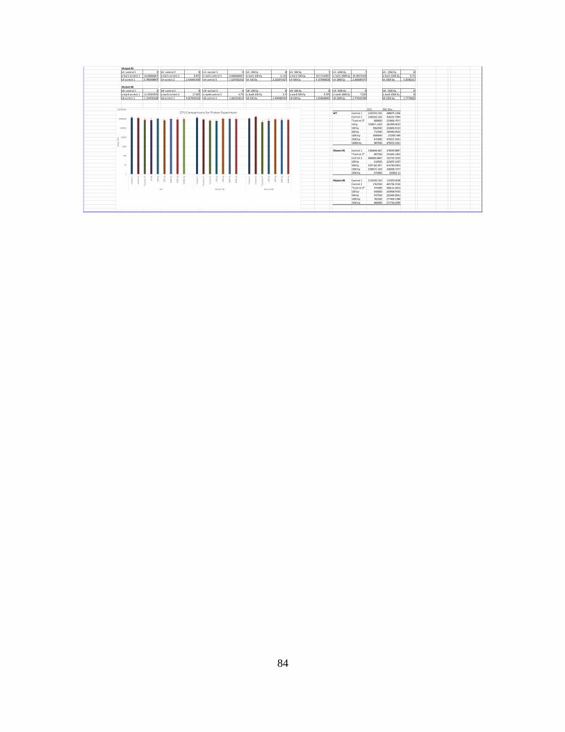
84
Mutant #5n5 -control 1 3 n5 -control 2 8 n5 -control 3 3 n5 -100 Gy 8 n5- 500 Gy 7 n5 -1000 Gy 7 n5 - 2500 Gy 8x-bar5-control 1 13.66666667 x-bar5-control 2 8.875 x-bar5-control 3 6.666666667 x-bar5-100 Gy 6.125 x-bar5-500 Gy 10.57142857 x-bar5-1000 Gy 10.28571429 x-bar5-2500 Gy 9.75s5-control 1 3.785938897 s5-control 2 2.416461403 s5-control 3 1.527525232 s5-100 Gy 2.232071427 s5-500 Gy 4.157609203 s5-1000 Gy 2.360387377 s5-2500 Gy 5.2030211
Mutant #8n8 -control 1 3 n8 -control 2 8 n8 -control 3 4 n8 -100 Gy 8 n8- 500 Gy 8 n8 -1000 Gy 8 n8 - 2500 Gy 8x-bar8-control 1 11.33333333 x-bar8-control 2 17.625 x-bar8-control 3 4.75 x-bar8-100 Gy 6.5 x-bar8-500 Gy 9.375 x-bar8-1000 Gy 7.625 x-bar8-2500 Gy 8s8-control 1 1.154700538 s8-control 2 4.657942526 s8-control 3 2.061552813 s8-100 Gy 2.449489743 s8-500 Gy 2.924648941 s8-1000 Gy 2.774243784 s8-2500 Gy 2.7774603
CFU Std. Dev.WT Control 1 1433333.333 288675.1346
Control 2 1283333.333 426223.7284*Control 3* 800000 223606.797710 Gy 742857.1429 281999.6623100 Gy 1062500 232609.4213500 Gy 712500 195940.95321000 Gy 1000000 232992.9492500 Gy 875000 470372.193110000 Gy 987500 470372.1931
Mutant #5 Control 1 1366666.667 378593.8897*Control 2* 887500 241646.1403Control 3 666666.6667 152752.5232100 Gy 612500 223207.1427500 Gy 1057142.857 415760.92031000 Gy 1028571.429 236038.73772500 Gy 975000 520302.11
Mutant #8 Control 1 1133333.333 115470.0538Control 2 1762500 465794.2526*Control 3* 475000 206155.2813100 Gy 650000 244948.9743500 Gy 937500 292464.89411000 Gy 762500 277424.37842500 Gy 800000 277746.0299
1
10
100
1000
10000
100000
1000000
10000000
Cont
rol 1
Cont
rol 2
*Con
trol
3*
10 G
y
100
Gy
500
Gy
1000
Gy
2500
Gy
1000
0 G
y
Cont
rol 1
*Con
trol
2*
Cont
rol 3
100
Gy
500
Gy
1000
Gy
2500
Gy
Cont
rol 1
Cont
rol 2
*Con
trol
3*
100
Gy
500
Gy
1000
Gy
2500
Gy
WT Mutant #5 Mutant #8
Tota
l CFU
CFU Comparisons for Proton Experiment
85
Bibliography
[1] D. R. Lewis, “711 HPW Research, Studies, Analysis, and Assessments Intramural
Proposal.” 2016. [2] H. Paganetti et al., “Relative biological effectiveness (RBE) values for proton
beam therapy,” Int. J. Radiat. Oncol., vol. 53, no. 2, pp. 407–421, 2002. [3] E. M. Bruch, A. de Groot, S. Un, and L. C. Tabares, “The effect of gamma-ray
irradiation on the Mn(II) speciation in Deinococcus radiodurans and the potential role of Mn(II)-orthophosphates,” Metallomics, vol. 7, no. 5, pp. 908–916, 2015.
[4] V. Mattimore and J. R. Battista, “Radioresistance of Deinococcus radiodurans: functions necessary to survive ionizing radiation are also necessary to survive prolonged desiccation.,” J. Bacteriol., vol. 178, no. 3, pp. 633–637, Feb. 1996.
[5] A. Krisko and M. Radman, “Biology of extreme radiation resistance: The way of Deinococcus radiodurans,” Cold Spring Harb. Perspect. Biol., vol. 5, no. 7, 2013.
[6] H. S. Misra, Y. S. Rajpurohit, and S. Kota, “Physiological and molecular basis of extreme radioresistance in Deinococcus radiodurans,” Curr. Sci., vol. 104, no. 2, pp. 194–205, 2013.
[7] E. L. Alpen, Radiation Biophysics, Second Edi. San Diego: Academic Press, 1990. [8] “DNA | Facts & Structure | Britannica.com.” [Online]. Available:
https://www.britannica.com/science/DNA. [Accessed: 04-Feb-2017]. [9] Y. M. Zhang, J. K. Liu, and T. Y. Wong, “The DNA excision repair system of the
highly radioresistant bacterium Deinococcus radiodurans is facilitated by the pentose phosphate pathway,” Mol. Microbiol., vol. 48, no. 5, pp. 1317–1323, 2003.
[10] M. Jaciuk, E. Nowak, K. Skowronek, A. Tańska, and M. Nowotny, “Structure of UvrA nucleotide excision repair protein in complex with modified DNA.,” Nat. Struct. Mol. Biol., vol. 18, no. 2, pp. 191–7, 2011.
[11] M. M. Cox, J. L. Keck, and J. R. Battista, “Rising from the ashes: DNA repair in Deinococcus radiodurans,” PLoS Genet., vol. 6, no. 1, pp. 1–2, 2010.
[12] K. Zahradka et al., “Reassembly of shattered chromosomes in Deinococcus radiodurans.,” Nature, vol. 443, no. 7111, pp. 569–73, 2006.
[13] K. R. Winchell, P. W. Egeler, A. J. VanDuinen, L. B. Jackson, M. E. Karpen, and P. D. Cook, “A Structural, Functional, and Computational Analysis of BshA, the First Enzyme in the Bacillithiol Biosynthesis Pathway.,” Biochemistry, vol. 55, no. 33, pp. 4654–65, Aug. 2016.
[14] A. T. Inc, “DD109.1,” 2016. [Online]. Available: http://www.adelphitech.com/products/dd109-1.html. [Accessed: 01-May-2016].
[15] J. Clinton and B. Singleton, “Laboratory Exercise 7: Neutron Detection and Measurement.” Wright Patterson Airforce Base, 2017.
[16] H. Cember, Introduction to Health Physics, 3rd Editio. New York: McGraw-Hill, 1996.
[17] I. Gla et al., “Survival of Deinococcus radiodurans Against Laboratory-Simulated Solar Wind Charged Particles,” vol. 11, no. 9, pp. 875–882, 2011.
[18] “Evaluated Nuclear Data File (ENDF).” [Online]. Available: http://www.nndc.bnl.gov/exfor/endf00.jsp. [Accessed: 05-Feb-2017].
86
[19] S. N. Laboratory, “Ion Beam Laboratory.” [Online]. Available: http://www.sandia.gov/research/facilities/technology_deployment_centers/ion_beam_lab/. [Accessed: 01-Jan-2017].
[20] J. Zeigler, “SRIM-The Stopping and Range of Ions in Matter.” [Online]. Available: http://www.srim.org/.
[21] J. T. Mclave, P. G. Benson, and T. Sincich, Statistics for Business and Economics, 12th ed. Pearson, 2014.
[22] L. Vysin et al., “Proton-induced direct and indirect damage of plasmid DNA,” Radiat. Environ. Biophys., vol. 54, no. 3, pp. 343–352, 2015.
[23] K. W. Minton and M. J. Daly, “A model for repair of radiation-induced DNA double-strand breaks in the extreme radiophile Deinococcus radiodurans,” BioEssays, vol. 17, no. 5, pp. 457–464, 1995.
[24] “Research Reactor | Nuclear Reactor Lab.” [Online]. Available: https://reactor.osu.edu/research-reactor. [Accessed: 05-Feb-2017].
87
REPORT DOCUMENTATION PAGE Form Approved OMB No. 074-0188
The public reporting burden for this collection of information is estimated to average 1 hour per response, including the time for reviewing instructions, searching existing data sources, gathering and maintaining the data needed, and completing and reviewing the collection of information. Send comments regarding this burden estimate or any other aspect of the collection of information, including suggestions for reducing this burden to Department of Defense, Washington Headquarters Services, Directorate for Information Operations and Reports (0704-0188), 1215 Jefferson Davis Highway, Suite 1204, Arlington, VA 22202-4302. Respondents should be aware that notwithstanding any other provision of law, no person shall be subject to an penalty for failing to comply with a collection of information if it does not display a currently valid OMB control number. PLEASE DO NOT RETURN YOUR FORM TO THE ABOVE ADDRESS. 1. REPORT DATE (DD-MM-YYYY)
21-02-2017 2. REPORT TYPE
Master’s Thesis 3. DATES COVERED (From – To)
March 2016 – March 2017
TITLE AND SUBTITLE Characterization of neutron and proton exposure on the radiation resistant bacterium, deinococcus radiodurans
5a. CONTRACT NUMBER
5b. GRANT NUMBER 5c. PROGRAM ELEMENT NUMBER
6. AUTHOR(S) Lenker, Ronald C., Major, USA
5d. PROJECT NUMBER
5e. TASK NUMBER
5f. WORK UNIT NUMBER
7. PERFORMING ORGANIZATION NAMES(S) AND ADDRESS(S) Air Force Institute of Technology Graduate School of Engineering and Management (AFIT/ENP) 2950 Hobson Way, Building 640 WPAFB OH 45433-8865
8. PERFORMING ORGANIZATION REPORT NUMBER AFIT-ENP-MS-17-M-100
9. SPONSORING/MONITORING AGENCY NAME(S) AND ADDRESS(ES) AFIT/Faculty Research Council 2950 Hobson Way Wright-Patterson AFB, OH 45433-7765 937-255-3633 ATTN: Office of Research and Sponsored Program
10. SPONSOR/MONITOR’S ACRONYM(S) AFRL/RHIQ (example) 11. SPONSOR/MONITOR’S REPORT NUMBER(S)
12. DISTRIBUTION/AVAILABILITY STATEMENT DISTRUBTION STATEMENT A. APPROVED FOR PUBLIC RELEASE; DISTRIBUTION UNLIMITED.
13. SUPPLEMENTARY NOTES This material is declared a work of the U.S. Government and is not subject to copyright protection in the United States. 14. ABSTRACT Deinococcus radiodurans is a robust bacterium that is known for its extraordinary resistance to ionizing radiation. In general, many of the investigations of this bacterium’s resistance have revolved around low linear energy transfer radiation, such as gamma and electron radiation. This study explored Deinococcus radiodurans’s ability to survive high linear energy transfer radiation, specifically proton and neutron radiation. Deinococcus radiodurans was dehydrated to reduce the effects of low linear energy transfer radiation. The bacteria were exposed to both neutron and proton radiation of varying amounts and rehydrated. The resulting colonies were counted and compared to colonies of non-irradiated control samples using a two population, t-statistic test. With few, non-trend forming exceptions, the results of these comparisons showed, with 95% certainty, that there was no statistical difference between the non-irradiated controls and the irradiated samples. 15. SUBJECT TERMS Deinococcus radiodurans, proton, neutron, linear energy transfer 16. SECURITY CLASSIFICATION OF:
17. LIMITATION OF ABSTRACT
UU
18. NUMBER OF PAGES
98
19a. NAME OF RESPONSIBLE PERSON LTC Douglas R. Lewis, AFIT/ENP
a. REPORT
U
b. ABSTRACT
U
c. THIS PAGE
U
19b. TELEPHONE NUMBER (Include area code) (937) 255-6565, ext 4569 ([email protected])
Standard Form 298 (Rev. 8-98) Prescribed by ANSI Std. Z39-18