Characterization of Natural Organic Matter in Drinking Water by

Fluorescence Spectroscopy

Cláudia Paiva e Cunha1

1Master Student in Biological Engineer at Instituto Superior Técnico Universidade de Lisboa, Av. Rovisco Pais 1, 1049-001 Lisboa,

Portugal

The main focus of this thesis was the use of fluorescence spectroscopy, in particular excitation emission matrices (EEMs) as a tool for characterization of natural organic matter in water samples. The extracted information could differentiate the waters according to their origin (surface or groundwater) and according to the treatment processes that had already undergone (raw or treated water).The reactivity of the chlorine was also evaluated, as maintaining residual chlorine concentrations between 0.2 and 1.0 mg/L in drinking water is a practice commonly used to ensure water quality and is a matter of human health. However, the chlorine concentration decays as the water travels through the systems due to chemical reactions between the disinfectant agent and natural organic matter (NOM) dissolved in the water. The wide diversity of compounds that constitute NOM intricate the study of these reactions and the use of advanced characterization tools, such as fluorescence spectroscopy, is essential to extract chemical information.

Keywords: Natural organic matter; Fluorescence spectroscopy; Excitation-emission matrices; Chlorine

INTRODUCTION Natural Organic Matter

Natural organic matter refers to a complex and diversified mixture of organic compounds that result from natural processes occuring in the environment. Dead and live plants, animals, microorganisms and their decomposition products may be the precursors of NOM (CHOW et al. 1999). Thus, NOM occurs as a consequence of the contact between water and dead or living organic matter present in the hydrological cycle (Bridgeman et al. 2011).

NOM is present in all fresh water sources, especially in surface waters and its composition varies in time and space, depending on the material that was in the basis of its genesis and the modifications it went through (Lankes et al. 2008). NOM prevenient from aquatic algae has high nitrogen content and the presence of aromatic carbon and phenolic compound is low, although terrestrially derived NOM has relatively low nitrogen content but large amounts of aromatic carbon and phenolic carbon (Fabris et al. 2008). This comparison proves NOM characteristics are intrinsically related with its origin. Besides its source, NOM concentration, composition and chemistry also depends on the physicochemical characteristics of the water column (e.g., pH, temperature, ionic strength), the surface chemistry of sediments and the occurrence of photolytic and microbiological degradation processes (Leenheer et al. 2003). NOM is not a passive agent in the aquatic system, playing multiple roles such as, acting as a carbon source for the metabolism of living organism and being an important part of ecological and geochemical functions, such as proton binding, influencing biogeochemical processes and photochemical reactions, transportation of inorganic

and organic substrates and aggregation and photochemical reactivity (Bridgeman et al. 2011).

Several studies have been conducted through the years in order to understand which the major components of NOM are and these include humic substances (HS). Humic substances are complex macromolecules and some consist in a mixture between many organic acids with variable functional groups as carboxylic and phenolic groups. HS contribute to 30 to 50 percent of the Dissolved Organic Carbon (DOC) in water (Thurman 1985). These multivariate groups can be divided in humic acids (HA) and fulvic acids (FA). The main difference between HA e FA is that HA are insoluble at pH less than 1, while FA are soluble at the all range of pH (Baghoth 2012). The non-humic fraction of organic matter or hydrophilic matter consists of less refractory molecules such as carbohydrates, proteins, sugars and aminoacids. Other compounds, such as amino acids, sugars and carboxylic acids are usually present in freshwaters although in smaller amounts, as well as a heterogeneous mixture of compounds that represent the hydrophilic acid fraction of dissolved organic matter (DOM) , also called “hydrophilic humic substances”(Thurman 1985).

Relevance in water systems

NOM presence is undesirable when it comes to drinking water due to aesthetic, operational and economical factors. The presence of some components causes a brownish yellow color and a disagreeable taste and odor (Leenheer et al. 2003). Moreover, NOM has the ability to act as a substrate,

promoting microbial growth and compromising the water safety. Hence, water abstracted from reservoirs and rivers (surface water) is treated in water treatment plants (WTP), where a large fraction of NOM is removed. However, treated water still has NOM in a variable concentration, depending on the initial NOM concentration and the effective removal capacity of the treatment plant. The removal of HS can be achieved using conventional methods for drinking water treatment, such as as flocculation, sedimentation and filtration. Removal of NOM of hydrophilic nature is more challenging. This fraction is a major contributor of easily biodegradable organic carbon, which promotes microbiological regrowth in the water distribution systems. There are some strategies that can be included in the treatment of potable water in order to remove the majority of NOM, however, some NOM characteristics, such as molecular weight distribution, carboxylic acidity and humic substances content may compromise the removal efficiency. Generally, high molecular weight compounds are easier to remove than low molecular weight components, especially the NOM fraction with MW of 500 Dalton (Da). NOM components with the highest carboxylic functionality and therefore, the highest charge density, show some resistance to removal by conventional treatment. Conventional treatment, direct filtration, and dissolved air flotation are some coagulation-based methods that can be used. The use of metal salts to induce NOM molecules to agglomerate, so that they can be removed using clarification or filtration, is also a valid alternative. Oxidation processes, such as ozonation, transform NOM into smaller and/or less reactive species that are less likely to form disinfection by-products (DBPs). High pressure membrane filtration processes can remove NOM molecules through size exclusion.

NOM may also compromise operational efficiency of treatment processes because it may foul membranes, block activated carbon pores and compete with taste and odors compounds for available adsorption sites, compromising the technique´s efficiency. The concentration of NOM that water contains may also influence the coagulant and disinfectant demand.

In order to combat waterborne diseases, different disinfectants are used to inactivate pathogens at the WTP, such as chlorine, ozone and chlorine dioxide. Chlorination of potable water is widely used worldwide because is economical viable and provides residual disinfecting capacity downstream from the treatment site. However, the use of chlorine does not eradicate Giardia and Cryptosporidium and the disinfectant reacts with NOM, leading to the appearance of potentially carcinogenic disinfection by-products, DBPs. This is the major concern related with the existence of NOM in WTP and in distribution systems. The reaction between NOM and disinfectant agents leads

to the formation of disinfection by-products and causes the decrease of disinfectant concentration, compromising water quality and safety (Matilainen et al. 2011). These by-products consist of trihalomethanes (THMs), haloacetic acids (HAAs), halo-acetonitriles (HANs) and other halogenated DBPs, and, due to its toxic and possibly carcinogenic nature, DBPs concentration obeys to a legal concentration limit. Moreover, NOM oxidation results on the formation of low weight compounds, which are easily assimilated by microorganisms (AOC – assimilable organic carbon), promoting microbiological growth in water systems, especially in the form of biofilms.

Reactivity of NOM towards chlorine

Chlorine is the most used disinfectant worldwide, and although it prevents waterborne diseases, it reacts with water’s NOM, leading to the formation of DBP’s and compromising the water safety for human health. Hence, prediction of NOM reactivity towards chlorine is a matter of public health.

Two distinct types of reactive functionalities exist in NOM resulting in two parallel first order reactions. One NOM

R functionality, possibly attributed to

aldehyde and phenolic hydroxyl groups, results in a very rapid rate of chlorine consumption. The other NOM

S functionality is less reactive, such as expected

for activated double bonds and methyl groups, and results in a slow, long-term chlorine consumption (Gang et al. 2003).

NOM reactivity to disinfectants is directly linked to its physical and chemical properties such as molecular weight (Cabaniss et al. 2000), aromaticity (Westerhoff et al. 1999), elemental composition and functional groups content (Perdue et al. 2003). According to Deborde et al. (2008), chlorine reactivity usually decreases in the following order: reduced sulfur components > primary and secondary amines > phenols and tertiary amines > double bonds, other aromatic components, carbonyls, amides. Nevertheless, (Korshin et al. 2007) refer to polyhydroxyaromatic (PHA) moieties as being the major chlorination sites in NOM, followed by esters and ketones.

Chlorine added to water disappears by four reaction types: oxidation, addition, substitution and catalyzed or light decomposition (Gang et al. 2003). According to (Kastl et al. 1999), most of the chlorine reacting in water is consumed by partial oxidation of NOM, while a small fraction of chlorine is consumed by the chlorination of organic compounds.

Measurement and Characterization of NOM

Several techniques can be used in order to measure and characterize NOM content in water samples. Total Organic Carbon (TOC) and Dissolved Organic Carbon (DOC) measurements are parameters

measured by standard analytical techniques largely used to determine the amount of organic carbon in a water sample. However, they only provide information about the amount of C atoms in the water samples and do not infer anything about the molecular structure of the substances they belong to. Operational parameters such as size, hydrophobicity and biodegradability can also be used to study NOM content in a water sample. Optic methods such as UV-Vis spectroscopy and fluorescence spectroscopy are also valuable techniques to infer about NOM structure. Regarding UV-Vis spectroscopy, in water samples, the inorganic chemicals do not absorb light significantly at wavelengths higher than 230 nm, whereas NOM components absorb in an extensive range of wavelengths. Therefore, light absorbance is a trustworthy semi-quantitative indicator of the concentration of NOM in natural waters (Li, Chi-Wang, Korshin, Gregory V, Benjamin 1997). In surface waters, absorbance is mainly attributed to aromatic chromophores, mostly humic, that are dissolved in the water (Leenheer et al. 2003). However, water spectra are broad and have no distinctive features (Leenheer et al. 2003) because they are the consequence of the superposition of the spectrum of many different chromophores, none of them possessing a particularly unique and discernible spectrum (Li, Chi-Wang, Korshin, Gregory V, Benjamin 1997; Perdue et al. 2003; Carter et al. 2012). Absorbance intensity at a single wavelength represents information at a specific point in the spectrum and, as such, is not a useful characteristic for structural understanding and highly limited for NOM characterization. Absorbance based-techniques are prone to have interference from several impediments present in water, such as UV-absorbing contaminations, pH, iron and nitrate. Thus, it is difficult to find a straight correlation between NOM reactivity and treatability parameters (i.e. reactivity with coagulants and disinfectants) based on absorbance-derived surrogates, because the results may only refer to a specific NOM fraction. This limitation can be overcome to a large extent by the use of fluorescence spectroscopy due to its sensitivity and selectivity (Bieroza et al. 2010).

In NOM, compounds which absorb light are known as chromophores and the ones which absorb and re-emit energy are called fluorophores. This intrinsic spectral property can be utilized in fingerprinting of NOM with fluorescence spectroscopy technique. With the recent technological advances in spectroscopy techniques, fluorescence spectroscopy has been received increased attention in the domain of drinking water treatment, because of its advantages such as fast, sensitive and selective NOM characterization, no need of a pre-treatment step, small sample volume and potential use for online monitoring (Bridgeman et al. 2011).

At room temperature, most molecules occupy the lowest vibrational level of the ground electronic

state (S0), however, when a light beam is absorbed, the molecules are elevated to generate excited states. Generally, the excited electronic state is usually the first excited singlet state (S1). Once the molecule is in a vibrational level of an electronic state, it rapidly loses the vibrational energy excess by collision and falls to the lowest vibrational level of the same electronic state. Every molecule that reside in an electronic level higher that the second suffers an internal conversion and collapses from the lowest vibrational level to the highest vibrational level of the electronic excited state immediately below, which has the same energy. From this point, the molecule loses energy until it reaches the lowest vibrational level of S1 for a period of nanoseconds, which is the fluorescence lifetime. Then, the molecule remains in the lowest vibrational level of S1, the molecule can return to any of the vibrational levels of the ground state, emitting its energy in the form of fluorescence. Fluorescence spectra are much more highly structured than absorbance spectra, often exhibiting several distinct maxima of fluorescence intensity with respect to both excitation and emission wavelength. Fluorescence techniques are widely used for NOM characterization in several types of waters (e.g., freshwaters, urban waters, seawater) (Stedmon et al. 2003; Chen et al. 2003; Bieroza et al. 2010; Carstea et al. 2010; Coble 1996; Hambly et al. 2010; Hudson et al. 2007; Peuravuori et al. 2002; Santos et al. 2009). These techniques have been used for monitoring and understanding NOM transformations in aquatic systems (Hudson et al. 2007), for the identification of the relative source of DOM (Rosario-Ortiz et al. 2007; Xu-jing et al. 2011), for the differentiation of NOM fractions (Marhaba et al. 2000; Chen et al. 2003) and for the identification of THM precursors (Hua et al. 2010).

Excitation-emission matrices (EEM) are the mostly used method to access NOM characteristics in several applications (Her et al. 2003; Hudson et al. 2007; Beggs et al. 2009; Carstea et al. 2010; Hambly et al. 2010; Seredynska-Sobecka et al. 2011). EEMs provide information on both the number and the type of fluorophores present as well as their abundance (Stedmon et al. 2003). This technique measures water sample´s fluorescence in a broad range of excitation and emission wavelengths. By simultaneously determining three fluorescence parameters, excitation wavelength, emission wavelength and fluorescence intensity, it is possible to obtain the entire fluorescence profile of a water sample. The results are arranged in a grid (excitation x emission x intensity) and the measured peak intensity is directly related to the concentration of the responsible fluorophore in the sample. EEM contains a considerable amount of information about NOM composition and structure and its interpretation allows a proper fingerprinting of water samples since specific excitation-emission wavelengths can be associated with a certain molecular conformation. Each EEM demonstrates a

specific combination of fluorescence intensities over a range of excitation and emission wavelengths. Thus, it is a much more explanatory technique than the single-scan methods (Bridgeman et al. 2011; Matilainen et al. 2011). EEMs are a very strong tool due to its non-destructivity of sample, and simplicity.

Excitation-Emission Matrices

NOM contains a variety of fluorophores and the two major NOM components that have been found to fluoresce are humic substances and protein-like substances (Coble 1996).

As said before, EEMs allow assessing the type of NOM that is dissolved in the water and can be easily interpreted if the intensity peaks are compared to the ranges of excitation and emission wavelengths of maximum intensity of fluorescence of pure compounds. Coble (1996) has suggested an alternative organization for the fluorescent regions: humic-like fluorescence consists of two peaks, one stimulated by UV excitation (peak A) and one by visible excitation (peak C), protein-like fluorescence is responsible for the appearance of peak B (tyrosine-like) and peak-T (tryptophan-like). According to McKnight et al. (2001), peak T can be used as an indicator of the aromaticity degree. 1 shows a fluorescence excitation-emission matrix with typical fluorescence features (peak A, C, B, T, Rayleigh-Tyndall effect and Raman scatter) as named by (Coble 1996).

Figure 1- Common EEM features and position of peaks A, C, B and T reported by (Coble 1996).

Adapted from (Hudson et al. 2007)

Quantitative analysis of EEM-Parallel Factor Analysis

Analysis of EEMs often requires the use of advanced statistical methods, being Parallel Factor Analysis (PARAFAC) the most used (Bro 1997). PARAFAC belongs to a family of multi-way methods used to explore data arranged in the form of a three-or higher-order array, which is the case of EEMs. PARAFAC of a three-way dataset decomposes the data signal into a set of trilinear terms and a residual array. PARAFAC is a multi-way method that provides both quantitative and qualitative information and facilitates the identification and quantification of

independent underlying signals, the components. Concerning the aim of this thesis, a three way array can be a matrix of sample x excitation x emission and, by using PARAFAC the three way dataset is splited in more specific three way arrays and a residual array. The following expression explains in a mathematical perspective PARAFAC inputs and outputs.

𝑥𝑖𝑗𝑘 = ∑ 𝑎𝑖𝑓𝑏𝑗𝑓𝑐𝑘𝑓 + 𝑒𝑖𝑗𝑘𝐹𝑓=1 𝑊ℎ𝑒𝑟𝑒 𝑖 =

1, … , 𝐼; 𝑗 = 1, … , 𝐽; 𝑘 = 1, … , 𝐾 (1)

In the case of EEMs, xijk symbolizes the fluorescence intensity of sample I, measured at the emission wavelength j and excitation wavelength k. The final term, eijk represents the unexplained signal, i.e., residuals that contain noise and other unmodeled variation. The model returns the parameters a, b and c, which, ideally, represent the concentration, emission and excitation spectra of the fluorophores. The equation above assumes that the fluorophores behave according the Lambert-Beer law and do not interact with each other. The measured signal is thus the sum of the contribution of each fluorophore (f).

Figure 2-EEMs of several samples splited into five

components (Murphy et al. 2013)

Each f corresponds to a PARAFAC component and every component as I a-values (scores), one for each sample. Each component also has J b-values, one for each emission wavelength as well as K c-values, one for each excitation wavelength. Only one fluorescence feature of the fluorophores varies and it is fluorescence intensity, which depends on its concentration in the respective sample. This means that the wavelength position of the fluorescence peaks of each fluorophore do not “shift,” however, the fluorescence maximum of the mixture will shift depending on the relative contribution (concentration) of each fluorophores (Stedmon et al. 2008).

EXPERIMENTAL SETUP AND PROCEDURES The general approach used for this work consisted on EEMs acquisition, lab-scale chlorination experiments with several water samples provided by two water utilities and EEMs analysis.It started with the development of a standardized procedure for EEM acquisition and correction with the existing spectrofluorometer. Then, several EEMs of waters samples from different sources and treatments were acquired and analyzed in order to identify the main fluorophores in each water and to test the ability of

this technique to assess the water’s NOM reactivity towards chlorine. Finally, a multi-way decomposition method (PARAFAC) was tested for quantitative analysis of the obtained EEMs and identification of NOM components that contribute to differences in fluorescence intensity.

Water Samples Water samples used were kindly provided by EPAL and Águas do Algarve. EPAL provided samples from Tagus River-Valada, Castelo do Bode dam, Ota and Lezíria. Samples from Odelouca dam were provided by Águas do Algarve. Tagus River-Valada, Castelo do Bode dam and Odelouca dam are from superficial abstractions and Lezíria and Ota are from underground abstractions.

In Asseiceira treatment plant, water from Castelo do Bode dam is treated according to the following treatment steps: pre-chlorination, remineralization, coagulation-flocculation-dissolved air flotation, ozonation, rapid sand filtration, pH adjustment and disinfection (chlorine). In Vale da Pedra treatment plant, water from Tagus River-Valada passes through several treatment steps: pre-chlorination, remineralization, coagulation-flocculation-sedimentation, rapid sand filtration, pH adjustment and disinfection (chlorine). The water collected in Ota and Lezíria wells is treated with gaseous chlorine.

Alcantarilha treatment plant receives water from Odelouca dam and the water treatment line is: pre-ozonation, coagulation-adsorption/flocculation/sedimentation, filtration and disinfection (chlorine).

Water samples were collected from different from different origins. Prior to all laboratory analyses, samples were stored cool in the dark.

Water samples handle In order to guarantee satisfactory outputs, a series of good laboratory practices have been established. All water samples were filtered in order to remove particles from the water samples, because particles can interfere with measurements and can also contain live organisms which produce or metabolize CDOM. Waters were filtered with hydrophilic polypropylene membrane filters with a pore size of 0.45 µm (PALL Corporation). Samples were stored refrigerated in the dark. Sample storage was made in suitable cleaned containers and samples were analyzed as soon as possible after sampling. Before every fluorescence reading in AquaLog®, the cuvette was washed with a solution of 0.5M of nitric acid (Merck, 65%) one time and three times with Milli-Q water. Gloves were used during samples handling.

Samples Chlorination Chlorination effect on NOM fluorescence was studied on three sets of experiments: the first set of experiments was conducted with real waters and an initial chlorine concentration of 1 mg/L, the second

batch was also conducted with real waters but with Cl/DOC of 3. In the third group of experiments was performed with the synthetic water samples diluted to 1mg C/L and Cl/DOC ratio of 3. In the first two experiments, the goal was to compare the EEM before chlorination with the EEM after chlorination. The third experiments aimed the evaluation of the fast and slow phase decay of chlorine. Samples were chlorinated with a NaClO stock solution (Panreac, 5% w/v QP). To determine chlorine concentration, 100 mL of Milli-Q water were chlorinated with a specific volume and the achieved concentration was measured according the DPD colorimetric method. During the experiments, samples were stored at 20 °C in an incubator (Leec, P3C).

Fluorescence Spectra Acquisition For the experiments described in this work, excitation-emission fluorescence matrices were recorded in a fluorospectrometer, AquaLog® from HORIBA Jobin Yvon Inc.. Aqualog® is the only instrument available in the market that simultaneously measures both absorbance spectra and fluorescence excitation-emission matrices in water quality analysis. Regarding this work, Aqualog® was used to develop excitation-emission matrices of multiple water samples: the spectroflurometer measures the fluorescence intensity at a specific excitation/emission pair and the information in rearranged in a three-dimensional matrix, where the x axis represents the excitation wavelength, emission wavelength is represented by the y axis and z axis relates with the absolute intensity values. The excitation range was from 240 to 450 nm and the emission wavelengths covered the range between 215 and 621 nm. In order to obtain representative EEMs, a study of the proper integration time was developed before every analysis. The EEMs were corrected for the inner-filter effect, Rayleigh and Raman scatters.

Qualitative Analysis The EEMs were analyzed regarding the existence of peaks C, A, B and T. Figure 1 was used as a model to evaluate the EEMs acquired.

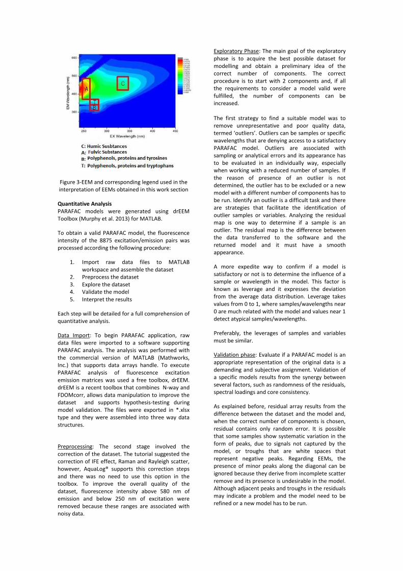
Figure 3-EEM and corresponding legend used in the interpretation of EEMs obtained in this work section

Quantitative Analysis PARAFAC models were generated using drEEM Toolbox (Murphy et al. 2013) for MATLAB.

To obtain a valid PARAFAC model, the fluorescence intensity of the 8875 excitation/emission pairs was processed according the following procedure:

1. Import raw data files to MATLAB workspace and assemble the dataset

2. Preprocess the dataset 3. Explore the dataset 4. Validate the model 5. Interpret the results

Each step will be detailed for a full comprehension of quantitative analysis.

Data Import: To begin PARAFAC application, raw data files were imported to a software supporting PARAFAC analysis. The analysis was performed with the commercial version of MATLAB (Mathworks, Inc.) that supports data arrays handle. To execute PARAFAC analysis of fluorescence excitation emission matrices was used a free toolbox, drEEM. drEEM is a recent toolbox that combines N-way and FDOMcorr, allows data manipulation to improve the dataset and supports hypothesis-testing during model validation. The files were exported in *.xlsx type and they were assembled into three way data structures.

Preprocessing: The second stage involved the correction of the dataset. The tutorial suggested the correction of IFE effect, Raman and Rayleigh scatter, however, AquaLog® supports this correction steps and there was no need to use this option in the toolbox. To improve the overall quality of the dataset, fluorescence intensity above 580 nm of emission and below 250 nm of excitation were removed because these ranges are associated with noisy data.

Exploratory Phase: The main goal of the exploratory phase is to acquire the best possible dataset for modelling and obtain a preliminary idea of the correct number of components. The correct procedure is to start with 2 components and, if all the requirements to consider a model valid were fulfilled, the number of components can be increased. The first strategy to find a suitable model was to remove unrepresentative and poor quality data, termed ‘outliers’. Outliers can be samples or specific wavelengths that are denying access to a satisfactory PARAFAC model. Outliers are associated with sampling or analytical errors and its appearance has to be evaluated in an individually way, especially when working with a reduced number of samples. If the reason of presence of an outlier is not determined, the outlier has to be excluded or a new model with a different number of components has to be run. Identify an outlier is a difficult task and there are strategies that facilitate the identification of outlier samples or variables. Analyzing the residual map is one way to determine if a sample is an outlier. The residual map is the difference between the data transferred to the software and the returned model and it must have a smooth appearance.

A more expedite way to confirm if a model is satisfactory or not is to determine the influence of a sample or wavelength in the model. This factor is known as leverage and it expresses the deviation from the average data distribution. Leverage takes values from 0 to 1, where samples/wavelengths near 0 are much related with the model and values near 1 detect atypical samples/wavelengths.

Preferably, the leverages of samples and variables must be similar.

Validation phase: Evaluate if a PARAFAC model is an appropriate representation of the original data is a demanding and subjective assignment. Validation of a specific models results from the synergy between several factors, such as randomness of the residuals, spectral loadings and core consistency.

As explained before, residual array results from the difference between the dataset and the model and, when the correct number of components is chosen, residual contains only random error. It is possible that some samples show systematic variation in the form of peaks, due to signals not captured by the model, or troughs that are white spaces that represent negative peaks. Regarding EEMs, the presence of minor peaks along the diagonal can be ignored because they derive from incomplete scatter remove and its presence is undesirable in the model. Although adjacent peaks and troughs in the residuals may indicate a problem and the model need to be refined or a new model has to be run.

A correct spectral appearance is also an indicator of the model aptness and when visualizing spectral loadings, some aspects need to be taken into account:

Ideally, the excitation and emission spectra cannot overlap more than 50 nm;

The excitation spectra can have various peaks, however, the emission spectra can only have one peak;

When an excitation spectrum has two or more peaks, indicating consecutive excited state absorption bands, some absorption (excitation) occurs between those peaks;

Excitation and emission spectra do not exhibit sudden changes at very close wavelengths.

This phase is not complete until the core consistency test is done. This test evaluates the appropriateness of the model and during this thesis the core consistency test was used as tie-breaking factor. When more than one model matched the criteria described above, was chosen the model with the highest core consistency percentage. Split half analysis is often used to confirm if the model is valid, however its application is datasets with few samples may not return positive outputs and this validation method was discarded in this quantitative analysis (Murphy et al. 2013).

RESULTS AND DISCUSSION

NOM characterization One goal of this study was to use fluorescence spectroscopy as a tool to differentiate water samples regarding their provenience (surface or groundwater) and the treatment steps that they have undergone (raw or treated waters). EEMs were obtained for water from Castelo do Bode (surface water and raw), Asseiceira (treated water from Castelo do Bode) and Lezíria-15 (groundwater), as figure 4 shows.

Figure 4-EEM of water sample from Castelo do Bode

and EEM of water sample from Asseceira

Analyzing the two EEMs, it is possible to see the effect of the conventional treatment, since the EEM of water sample from Asseiceira is less intense than EEM of water from Castelo do Bode. The more intense peak corresponds to the existence of humic

acids in both EEMs, however, in the second EEM the peak is less intense, since water from Asseiceira is less reactive that water from Castelo do Bode dam. It is possible to see that NOM a part of NOM was removed after the conventional treatment.

Figure 5 shows the EEMs obtained for surface and groundwater.

Figure 5- EEM of water sample from Castelo do Bode and EEM of water sample from Lezíria-15

The obvious difference between the two EEMs is the location of the most intense peak. In Castelo do Bode water sample, peak A, associated with the existence of humic acids, show the highest fluorescence intensity. In EEM of water from Lezíria-15, aminoacids seems to be the most relevant components, since peak B and T have the highest fluorescence intensities.

EEMs are a valuable tool to distinguish between raw and treated waters and surface and groundwater, since NOM fluorescence profile depends on the water origin and on the treatment steps applied.

Initial chlorine concentration of 1.0 mg/L In order to study and identify NOM fractions that show potential to react with chlorine, a chlorine decay experiment was conducted. Figure 6 and Figure 7 show the EEMs obtained before and after chlorination with two different waters.

Figure 6-EEMs of water from Lezíria-15, before and after chlorination. Lezíria-15 is a groundwater with

pH of 7.7 and DOC of 0.37 ppm

Analyzing Figure 4, the effect of chlorine is visible, since the second EEM does not exhibit the presence of NOM. The initial chlorine concentration was sufficient to promote the oxidation of NOM that fluoresces.

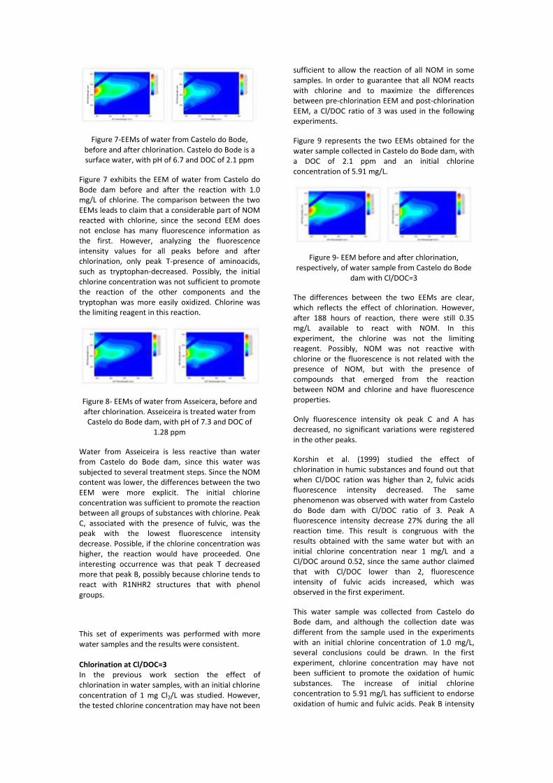
Figure 7-EEMs of water from Castelo do Bode, before and after chlorination. Castelo do Bode is a surface water, with pH of 6.7 and DOC of 2.1 ppm

Figure 7 exhibits the EEM of water from Castelo do Bode dam before and after the reaction with 1.0 mg/L of chlorine. The comparison between the two EEMs leads to claim that a considerable part of NOM reacted with chlorine, since the second EEM does not enclose has many fluorescence information as the first. However, analyzing the fluorescence intensity values for all peaks before and after chlorination, only peak T-presence of aminoacids, such as tryptophan-decreased. Possibly, the initial chlorine concentration was not sufficient to promote the reaction of the other components and the tryptophan was more easily oxidized. Chlorine was the limiting reagent in this reaction.

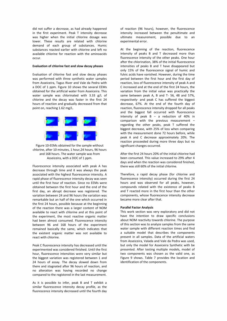
Figure 8- EEMs of water from Asseicera, before and after chlorination. Asseiceira is treated water from Castelo do Bode dam, with pH of 7.3 and DOC of

1.28 ppm

Water from Asseiceira is less reactive than water from Castelo do Bode dam, since this water was subjected to several treatment steps. Since the NOM content was lower, the differences between the two EEM were more explicit. The initial chlorine concentration was sufficient to promote the reaction between all groups of substances with chlorine. Peak C, associated with the presence of fulvic, was the peak with the lowest fluorescence intensity decrease. Possible, if the chlorine concentration was higher, the reaction would have proceeded. One interesting occurrence was that peak T decreased more that peak B, possibly because chlorine tends to react with R1NHR2 structures that with phenol groups.

This set of experiments was performed with more water samples and the results were consistent. Chlorination at Cl/DOC=3 In the previous work section the effect of chlorination in water samples, with an initial chlorine concentration of 1 mg Cl2/L was studied. However, the tested chlorine concentration may have not been

sufficient to allow the reaction of all NOM in some samples. In order to guarantee that all NOM reacts with chlorine and to maximize the differences between pre-chlorination EEM and post-chlorination EEM, a Cl/DOC ratio of 3 was used in the following experiments.

Figure 9 represents the two EEMs obtained for the water sample collected in Castelo do Bode dam, with a DOC of 2.1 ppm and an initial chlorine concentration of 5.91 mg/L.

Figure 9- EEM before and after chlorination, respectively, of water sample from Castelo do Bode

dam with Cl/DOC=3

The differences between the two EEMs are clear, which reflects the effect of chlorination. However, after 188 hours of reaction, there were still 0.35 mg/L available to react with NOM. In this experiment, the chlorine was not the limiting reagent. Possibly, NOM was not reactive with chlorine or the fluorescence is not related with the presence of NOM, but with the presence of compounds that emerged from the reaction between NOM and chlorine and have fluorescence properties.

Only fluorescence intensity ok peak C and A has decreased, no significant variations were registered in the other peaks.

Korshin et al. (1999) studied the effect of chlorination in humic substances and found out that when Cl/DOC ration was higher than 2, fulvic acids fluorescence intensity decreased. The same phenomenon was observed with water from Castelo do Bode dam with Cl/DOC ratio of 3. Peak A fluorescence intensity decrease 27% during the all reaction time. This result is congruous with the results obtained with the same water but with an initial chlorine concentration near 1 mg/L and a Cl/DOC around 0.52, since the same author claimed that with Cl/DOC lower than 2, fluorescence intensity of fulvic acids increased, which was observed in the first experiment.

This water sample was collected from Castelo do Bode dam, and although the collection date was different from the sample used in the experiments with an initial chlorine concentration of 1.0 mg/L, several conclusions could be drawn. In the first experiment, chlorine concentration may have not been sufficient to promote the oxidation of humic substances. The increase of initial chlorine concentration to 5.91 mg/L has sufficient to endorse oxidation of humic and fulvic acids. Peak B intensity

did not suffer a decrease, as had already happened in the first experiment. Peak T intensity decrease was higher when the initial chlorine dosage was lower. These results are related with chlorine demand of each group of substances. Humic substances reacted earlier with chlorine and left no available chlorine for reaction with the aminoacids occur.

Evaluation of chlorine fast and slow decay phases Evaluation of chlorine fast and slow decay phases was performed with three synthetic water samples from Asseiceira, Tagus River and Vale da Pedra with a DOC of 1 ppm. Figure 10 shows the sevaral EEMs obtained for the artificial water from Asseiceira. This water sample was chlorinated with 3.33 g/L of chlorine and the decay was faster in the first 24 hours of reaction and gradually decreased from that point on, reaching 1.62 mg/L.

Figure 10-EEMs obtained for the sample without

chlorine, after 10 minutes, 1 hour,24 hours, 96 hours and 168 hours. The water sample was from

Asseiceira, with a DOC of 1 ppm.

Fluorescence intensity associated with peak A has decrease through time and it was always the peak associated with the highest fluorescence intensity. A rapid phase of fluorescence intensity decay was seen until the first hour of reaction. Since no EEMs were obtained between the first hour and the end of the first day, an abrupt decrease was registered. The variation between 24 and 96 hours the variation was remarkable but an half of the one which occurred in the first 24 hours, possible because at the beginning of the reaction there was a larger content of NOM available to react with chlorine and at this point of the experiment, the most reactive organic matter had been almost consumed. Fluorescence intensity between 96 and 168 hours of the experiment remained basically the same, which indicates that the existent organic matter was not available to react with chlorine.

Peak C fluorescence intensity has decreased until the experimented was considered finished. Until the first hour, fluorescence intensities were very similar but the biggest variation was registered between 1 and 24 hours of assay. The decay slowed down from there and stagnated after 96 hours of reaction, and no alteration was having recorded no change compared to the registered in the last measurement.

As it is possible to infer, peak B and T exhibit a similar fluorescence intensity decay profile, as the fluorescence intensity decreased until the fourth day

of reaction (96 hours), however, the fluorescence intensity increased between the penultimate and ultimate measurement, possible due to an experimental error.

At the beginning of the reaction, fluorescence intensity of peaks B and T decreased more than fluorescence intensity of the other peaks. One hour after the chlorination, 38% of the initial fluorescence intensities of peaks B and T have disappeared but only 15% of the fluorescence signal of humic and fulvic acids have vanished. However, during the time period between the first hour and the first day of reaction, loss of fluorescence intensity of peak A and C increased and at the end of the first 24 hours, the variation from the initial value was practically the same between peak A, B and T- 56, 48 and 57%, respectively- and peak C has suffered the biggest decrease, 67%. At the end of the fourth day of reaction, fluorescence intensity dropped for all peaks and the biggest fall occurred with fluorescence intensity of peak B – a reduction of 40% in comparison with the previous measurement – regarding the other peaks, peak T suffered the biggest decrease, with 25% of loss when comparing with the measurement done 72 hours before, while peak A and C decrease approximately 20%. The reaction proceeded during more three days but no significant changes occurred.

After the first 24 hours 20% of the initial chlorine had been consumed. This value increased to 29% after 4 days and when the reaction was considered finished, there was still 60% of the initial chlorine.

Therefore, a rapid decay phase (for chlorine and fluorescence intensity) occurred during the first 24 hours and was observed for all peaks, however, compounds related with the existence of peaks B and T reacted more in the first hour than the other components, whose fluorescence intensity decrease became more clear after that.

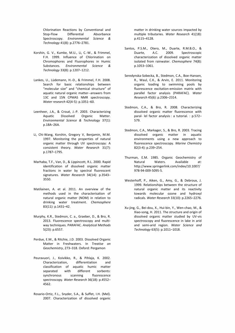
Parallel Factor Analysis This work section was very exploratory and did not have the intention to draw specific conclusions about NOM reactivity towards chlorine. The purpose of this section was to analyze samples from the same water sample with different reaction times and find a suitable model that describes the components present in all samples. Data of the artificial waters from Asseiceira, Valada and Vale da Pedra was used, but only the model for Asseiceira Synthetic with be presented. After testing multiple models, model of two components was chosen as the valid one, as Figure 9 shows. Table 7 provides the location and identification of the components.

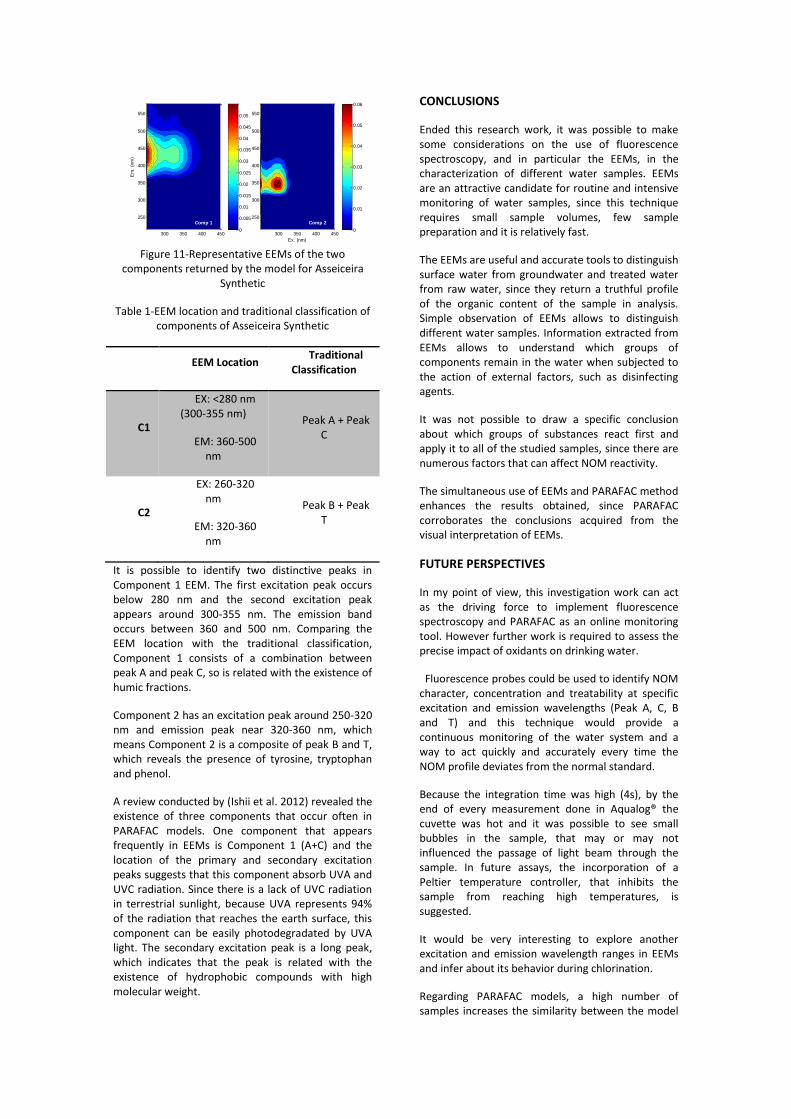
Figure 11-Representative EEMs of the two components returned by the model for Asseiceira

Synthetic

Table 1-EEM location and traditional classification of components of Asseiceira Synthetic

EEM Location Traditional

Classification

C1

EX: <280 nm (300-355 nm)

EM: 360-500 nm

Peak A + Peak C

C2

EX: 260-320 nm

EM: 320-360 nm

Peak B + Peak T

It is possible to identify two distinctive peaks in Component 1 EEM. The first excitation peak occurs below 280 nm and the second excitation peak appears around 300-355 nm. The emission band occurs between 360 and 500 nm. Comparing the EEM location with the traditional classification, Component 1 consists of a combination between peak A and peak C, so is related with the existence of humic fractions.

Component 2 has an excitation peak around 250-320 nm and emission peak near 320-360 nm, which means Component 2 is a composite of peak B and T, which reveals the presence of tyrosine, tryptophan and phenol.

A review conducted by (Ishii et al. 2012) revealed the existence of three components that occur often in PARAFAC models. One component that appears frequently in EEMs is Component 1 (A+C) and the location of the primary and secondary excitation peaks suggests that this component absorb UVA and UVC radiation. Since there is a lack of UVC radiation in terrestrial sunlight, because UVA represents 94% of the radiation that reaches the earth surface, this component can be easily photodegradated by UVA light. The secondary excitation peak is a long peak, which indicates that the peak is related with the existence of hydrophobic compounds with high molecular weight.

CONCLUSIONS

Ended this research work, it was possible to make some considerations on the use of fluorescence spectroscopy, and in particular the EEMs, in the characterization of different water samples. EEMs are an attractive candidate for routine and intensive monitoring of water samples, since this technique requires small sample volumes, few sample preparation and it is relatively fast.

The EEMs are useful and accurate tools to distinguish surface water from groundwater and treated water from raw water, since they return a truthful profile of the organic content of the sample in analysis. Simple observation of EEMs allows to distinguish different water samples. Information extracted from EEMs allows to understand which groups of components remain in the water when subjected to the action of external factors, such as disinfecting agents.

It was not possible to draw a specific conclusion about which groups of substances react first and apply it to all of the studied samples, since there are numerous factors that can affect NOM reactivity.

The simultaneous use of EEMs and PARAFAC method enhances the results obtained, since PARAFAC corroborates the conclusions acquired from the visual interpretation of EEMs.

FUTURE PERSPECTIVES

In my point of view, this investigation work can act as the driving force to implement fluorescence spectroscopy and PARAFAC as an online monitoring tool. However further work is required to assess the precise impact of oxidants on drinking water.

Fluorescence probes could be used to identify NOM character, concentration and treatability at specific excitation and emission wavelengths (Peak A, C, B and T) and this technique would provide a continuous monitoring of the water system and a way to act quickly and accurately every time the NOM profile deviates from the normal standard.

Because the integration time was high (4s), by the end of every measurement done in Aqualog® the cuvette was hot and it was possible to see small bubbles in the sample, that may or may not influenced the passage of light beam through the sample. In future assays, the incorporation of a Peltier temperature controller, that inhibits the sample from reaching high temperatures, is suggested.

It would be very interesting to explore another excitation and emission wavelength ranges in EEMs and infer about its behavior during chlorination.

Regarding PARAFAC models, a high number of samples increases the similarity between the model

Comp 1

Em

. (n

m)

300 350 400 450

250

300

350

400

450

500

550

Comp 2

Ex. (nm)

300 350 400 450

250

300

350

400

450

500

550

0

0.005

0.01

0.015

0.02

0.025

0.03

0.035

0.04

0.045

0.05

0

0.01

0.02

0.03

0.04

0.05

0.06

and the original data, and it would be recommend to generate a model with the largest possible number of samples.

REFERENCES

Baghoth, S.A. 2012. Characterizing natural organic matter in drinking water treatment processes and trains. UNESCO-IHE Institute for Water Education.

Beggs, K.M.H., Summers, R.S., & McKnight, D.M. 2009. Characterizing chlorine oxidation of dissolved organic matter and disinfection by-product formation with fluorescence spectroscopy and parallel factor analysis. Journal of Geophysical Research 114(G4): p.G04001.

Bieroza, M.Z., Bridgeman, J., & Baker, a. 2010. Fluorescence spectroscopy as a tool for determination of organic matter removal efficiency at water treatment works. Drinking Water Engineering and Science 3(1): p.63–70..

Bridgeman, J., Bieroza, M., & Baker, A. 2011. The application of fluorescence spectroscopy to organic matter characterisation in drinking water treatment. Reviews in Environmental Science and Bio/Technology 10(3): p.277–290. Bro, R. 1997. PARAFAC . Tutorial and applications. 38: p.149–171.

Cabaniss, S.E., Zhou, Q., Maurice, P.A., Chin, Y.-P., & Aiken, G.R. 2000. A Log-Normal Distribution Model for the Molecular Weight of Aquatic Fulvic Acids. Environmental Science & Technology 34(6): p.1103–1109.

Carstea, E.M., Baker, A., Bieroza, M., & Reynolds, D. 2010. Continuous fluorescence excitation-emission matrix monitoring of river organic matter. Water research 44(18): p.5356–66.

Carter, H.T. et al. 2012. Freshwater DOM quantity and quality from a two-component model of UV absorbance. Water research 46(14): p.4532–42. Chen, J., LeBoeuf, E.J., Dai, S., & Gu, B. 2003. Fluorescence spectroscopic studies of natural organic matter fractions. Chemosphere 50(5): p.639–47.

CHOW, C. et al. 1999. The impact of the character of natural organic matter in conventional treatment with alum. Water Science and Technology 40(9): p.97–104. Coble, P.G. 1996. Characterization of marine and terrestrial DOM in seawater using excitation-emission matrix spectroscopy. Marine Chemistry 51(4): p.325–346.

Deborde, M., & von Gunten, U. 2008. Reactions of chlorine with inorganic and organic compounds during water treatment--Kinetics and mechanisms: A critical review. Water Research 42(1-2): p.13–51.

Fabris, R., Chow, C.W.K., Drikas, M., & Eikebrokk, B. 2008. Comparison of NOM character in selected Australian and Norwegian drinking waters. Water research 42(15): p.4188–96. Available at: http://www.ncbi.nlm.nih.gov/pubmed/18706670 [Accessed February 11, 2014].

Gang, D., Clevenger, T.E., & Banerji, S.K. 2003. Modeling Chlorine Decay in Surface Water. Journal of Environmental Informatics 1(1): p.21–27.

Hambly, A.C. et al. 2010. Fluorescence monitoring at a recycled water treatment plant and associated dual distribution system - Implications for cross-connection detection. Water Research 44(18): p.5323–5333.

Her, N., Amy, G., McKnight, D., Sohn, J., & Yoon, Y. 2003. Characterization of DOM as a function of MW by fluorescence EEM and HPLC-SEC using UVA, DOC, and fluorescence detection. Water research 37(17): p.4295–303.

Hua, B., Veum, K., Yang, J., Jones, J., & Deng, B. 2010. Parallel factor analysis of fluorescence EEM spectra to identify THM precursors in lake waters. Environmental monitoring and assessment 161(1-4): p.71–81.

Hudson, N., Baker, A., & Reynolds, D. 2007. Fluorescence analysis of dissolved organic matter in natural, waste and polluted waters—a review. River Research and Applications 23(6): p.631–649.

Ishii, S.K.L., & Boyer, T.H. 2012. Critical Review.

Kastl, G.J., Fisher, I.H., & Jegatheesan, V. 1999. Evaluation of chlorine decay kinetics expressions for drinking water distribution systems modelling. Journal of Water Supply: Research and Technology - Aqua 48(6): p.219–226.

Korshin, G. V., Benjamin, M.M., Chang, H.-S., & Gallard, H. 2007. Examination of NOM

Chlorination Reactions by Conventional and Stop-Flow Differential Absorbance Spectroscopy. Environmental Science & Technology 41(8): p.2776–2781.

Korshin, G. V., Kumke, M.U., Li, C.-W., & Frimmel, F.H. 1999. Influence of Chlorination on Chromophores and Fluorophores in Humic Substances. Environmental Science & Technology 33(8): p.1207–1212.

Lankes, U., Lüdemann, H.-D., & Frimmel, F.H. 2008. Search for basic relationships between “molecular size” and “chemical structure” of aquatic natural organic matter--answers from 13C and 15N CPMAS NMR spectroscopy. Water research 42(4-5): p.1051–60.

Leenheer, J.A., & Croué, J.-P. 2003. Characterizing Aquatic Dissolved Organic Matter. Environmental Science & Technology 37(1): p.18A–26A.

Li, Chi-Wang, Korshin, Gregory V, Benjamin, M.M. 1997. Monitoring the properties of natural organic matter through UV spectroscopy: A consistent theory. Water Research 31(7): p.1787–1795.

Marhaba, T.F., Van, D., & Lippincott, R.L. 2000. Rapid identification of dissolved organic matter fractions in water by spectral fluorescent signatures. Water Research 34(14): p.3543–3550.

Matilainen, A. et al. 2011. An overview of the methods used in the characterisation of natural organic matter (NOM) in relation to drinking water treatment. Chemosphere 83(11): p.1431–42.

Murphy, K.R., Stedmon, C. a., Graeber, D., & Bro, R. 2013. Fluorescence spectroscopy and multi-way techniques. PARAFAC. Analytical Methods 5(23): p.6557.

Perdue, E.M., & Ritchie, J.D. 2003. Dissolved Organic Matter in Freshwaters. In Treatise on Geochemistry, 273–318. Oxford: Pergamon

Peuravuori, J., Koivikko, R., & Pihlaja, K. 2002. Characterization, differentiation and classification of aquatic humic matter separated with different sorbents: synchronous scanning fluorescence spectroscopy. Water Research 36(18): p.4552–4562.

Rosario-Ortiz, F.L., Snyder, S.A., & Suffet, I.H. (Mel). 2007. Characterization of dissolved organic

matter in drinking water sources impacted by multiple tributaries. Water Research 41(18): p.4115–4128.

Santos, P.S.M., Otero, M., Duarte, R.M.B.O., & Duarte, A.C. 2009. Spectroscopic characterization of dissolved organic matter isolated from rainwater. Chemosphere 74(8): p.1053–1061.

Seredynska-Sobecka, B., Stedmon, C.A., Boe-Hansen, R., Waul, C.K., & Arvin, E. 2011. Monitoring organic loading to swimming pools by fluorescence excitation-emission matrix with parallel factor analysis (PARAFAC). Water Research 45(6): p.2306–2314.

Stedmon, C.A., & Bro, R. 2008. Characterizing dissolved organic matter fluorescence with paral- lel factor analysis : a tutorial. : p.572–579.

Stedmon, C.A., Markager, S., & Bro, R. 2003. Tracing dissolved organic matter in aquatic environments using a new approach to fluorescence spectroscopy. Marine Chemistry 82(3-4): p.239–254.

Thurman, E.M. 1985. Organic Geochemistry of Natural Waters. Available at: http://www.springerlink.com/index/10.1007/978-94-009-5095-5.

Westerhoff, P., Aiken, G., Amy, G., & Debroux, J. 1999. Relationships between the structure of natural organic matter and its reactivity towards molecular ozone and hydroxyl radicals. Water Research 33(10): p.2265–2276.

Xu-jing, G., Bei-dou, X., Hui-bin, Y., Wen-chao, M., & Xiao-song, H. 2011. The structure and origin of dissolved organic matter studied by UV-vis spectroscopy and fluorescence in lake in arid and semi-arid region. Water Science and Technology 63(5): p.1011–1018.