characterization of high intensity focused ultrasound ... of high intensity focused ultrasound...

Characterization of high intensity focused ultrasoundtransducers using acoustic streaming

Prasanna HariharanDivision of Solid and Fluid Mechanics, Center for Devices and Radiological Health, U. S. Foodand Drug Administration, Silver Spring, Maryland 20993, USA and Mechanical, Industrial, and NuclearEngineering Department, University of Cincinnati, Cincinnati, Ohio 45221, USA

Matthew R. Myers,a� Ronald A. Robinson, and Subha H. MaruvadaDivision of Solid and Fluid Mechanics, Center for Devices and Radiological Health, U. S. Foodand Drug Administration, Silver Spring, Maryland 20993, USA

Jack SliwaSt. Jude Medical, AF Division, 240 Santa Ana Court, Sunnyvale, California 94085, USA

Rupak K. BanerjeeMechanical, Industrial and Nuclear Engineering Department and Biomedical Engineering Department,598 Rhodes Hall, P.O. Box 210072, University of Cincinnati, Cincinnati, Ohio 45221, USA

�Received 3 August 2007; revised 20 December 2007; accepted 26 December 2007�

A new approach for characterizing high intensity focused ultrasound �HIFU� transducers ispresented. The technique is based upon the acoustic streaming field generated by absorption of theHIFU beam in a liquid medium. The streaming field is quantified using digital particle imagevelocimetry, and a numerical algorithm is employed to compute the acoustic intensity field givingrise to the observed streaming field. The method as presented here is applicable to moderateintensity regimes, above the intensities which may be damaging to conventional hydrophones, butbelow the levels where nonlinear propagation effects are appreciable. Intensity fields and acousticpowers predicted using the streaming method were found to agree within 10% with measurementsobtained using hydrophones and radiation force balances. Besides acoustic intensity fields, thestreaming technique may be used to determine other important HIFU parameters, such as beam tiltangle or absorption of the propagation medium. © 2008 Acoustical Society of America.�DOI: 10.1121/1.2835662�

PACS number�s�: 43.80.Ev, 43.35.Yb, 43.25.Nm �CCC� Pages: 1706–1719

I. INTRODUCTION

Most therapeutic ultrasound procedures, including tumorablation, hemostasis, and gene activation, rely on the abilityof high intensity focused ultrasound �HIFU� to rapidly el-evate tissue temperatures. In order to maximize the effective-ness of the procedure, as well as to avoid collateral tissuedamage, it is desirable to predict the energy distribution ofthe HIFU beam within the propagation medium. An impor-tant first step in this process is the characterization of theultrasound beam in a liquid medium. In this characterization,the acoustic intensity is determined throughout the spatialvolume of interest, for transducer power levels of practicalimportance.

Currently, HIFU fields are often characterized using ra-diation force balance and hydrophone techniques, whichmeasure the ultrasonic power and intensity distribution, re-spectively �Shaw and ter Haar, 2006; Harris 2005�. Althoughthese two techniques are well established and widely used,there are known limitations to both of these methods, includ-ing: �i� sensor damage due to heating and cavitation; �ii�

inaccuracies due to strong focusing; and �iii� inaccurate fre-quency response due to generation of higher harmonics�Shaw and ter Haar, 2006�. Consequently, these techniquescan accurately characterize HIFU transducers only at lowpower. For clinically relevant high powers, there are no al-ternative measurement standards available to accuratelycharacterize medical ultrasound fields generated by HIFUtransducers �Shaw and ter Haar, 2006; Harris 2005�.

Several new methods for measuring HIFU fields are be-ing researched, including development of robust sensors andhydrophones �Wang et al., 1999; Shaw, 2004; Schafer et al.,2006; Zanelli and Howard, 2006; Shaw and ter Haar, 2006�.An alternative approach to overcome the sensor-induced in-accuracies is to eliminate the use of sensors, and noninva-sively measure the pressure field. One such commerciallyavailable noninvasive method is the schlieren imaging tech-nique �Harland et al., 2002; Theobald et al., 2004�, whichutilizes changes in the optical index of refraction to qualita-tively define the ultrasound field. However, for quantitativeevaluation, the pressure field must be reconstructed tomo-graphically. Other than schlieren imaging, there are no non-intrusive techniques reported in recent literature capable ofmeasuring ultrasound field at high powers.

a�Author to whom correspondence should be addressed. Electronic mail:[email protected]

1706 J. Acoust. Soc. Am. 123 �3�, March 2008 © 2008 Acoustical Society of America0001-4966/2008/123�3�/1706/14/$23.00

This paper describes a noninvasive method that is ca-pable of measuring the acoustic intensity in a free field. Themethod incorporates acoustic streaming, the steady fluidmovement generated when propagating acoustic waves areattenuated by viscosity of the fluid medium �Nyborg, 1965�.Acoustic streaming arising from ultrasound absorption wasfirst discussed by Eckart �1948�, who derived an expressionfor the streaming velocity by applying the method of succes-sive approximations to the Navier-Stokes equations. Accord-ing to Eckart’s theory, the acoustic streaming velocity is di-rectly proportional to the square of acoustic pressure, andinversely proportional to the shear viscosity. However, Eck-art’s expression was derived ignoring the hydrodynamic non-linearity term in the Navier-Stokes equation. Later, Lighthill�1978a, b� established that this steady streaming motion isdue to the mean momentum flux �Reynolds stress� created bythe viscous dissipation of acoustic energy in the fluid me-dium. Subsequently, Starritt et al. �1989, 1991�, Tjotta andTjotta �1993�, and Kamakura et al. �1995� investigated, bothexperimentally and numerically, the effect of acoustic andhydrodynamic nonlinearity on the streaming velocity for afocused ultrasound source. Results obtained from their ex-periments and computations suggest that both acoustic andhydrodynamic nonlinearities can play a major role in genera-tion of acoustic streaming.

Previous studies have exploited the relationship betweenthe acoustic streaming field and the ultrasound intensity tovarious degrees. Nowicki et al. �1998� used both particleimage velocimetry �PIV� and Doppler ultrasound to measurestreaming motion generated by a weakly focused ultrasoundbeam in a solution of water and cornstarch. They found thatsimilar streaming velocities were obtained for both the meth-ods and the velocity magnitude was directly proportional tothe acoustic power emitted by the transducer. Hartley et al.�1997� and Shi et al. �2002�used Doppler ultrasound to quan-titatively measure acoustic streaming velocity in blood whenexposed to an ultrasound source. They used streaming as apotential tool for improving hemorrhage diagnosis. Hartleyet al. �1997� found that the streaming velocity increases withacoustic power and reduces with increase in viscosity duringblood coagulation. Choi et al. �2004� used PIV to character-ize streaming motion induced by a lithotripter. They ob-served that the streaming velocity correlated linearly with thepeak negative pressure of the acoustic field measured at thefocus. More recently, Madelin et al. �2006� used MRI tomeasure streaming velocity in a Glycerol water mixture.From the streaming velocity they tried to estimate the fluidproperties such as attenuation and bulk viscosity. They usedthe expression derived by Eckart �1948� to calculate theacoustic field and time-averaged acoustic power of a planeultrasound transducer from the streaming velocity data.While all of these experimental studies have observed a cor-relation between the acoustic intensity field �and acousticpower� and the acoustic streaming field, none of them at-tempted to use this correlation to accurately predict theacoustic intensity field.

Our characterization technique employs a predictor-corrector type method that back calculates the total ultra-sonic power and acoustic intensity field from the streaming

velocity field generated by the HIFU transducers. The acous-tic streaming field set up by the HIFU beam with unknownenergy distribution is measured experimentally using digitalparticle image velocimetry �DPIV� �Prasad, 2000�. Then, aninitial guess for the unknown acoustic intensity field is made.Based upon the Reynolds stress derived from this intensity,the streaming velocity is computed and compared with theexperimental values. Using the error between the computedand observed velocity fields, an optimization routine is em-ployed to refine the guess for the intensity field and the com-putation procedure is repeated. When the difference betweenthe computed and measured velocity fields falls below athreshold value, the final estimate for the ultrasound intensityfield is obtained. This inverse method can also be used toestimate physical properties of the fluid medium such as ul-trasound absorption coefficient, or properties of the beamsuch as tilt angle.

The acoustic intensities of interest in this paper are thosethat are low enough that nonlinear propagation may beneglected, yet high enough to produce temperature increasesin tissue of a few degrees per second. We label this rangethe “moderate” temperature regime �Hariharan et al., 2007�.An order-of-magnitude estimate of this regime is100–1000 W /cm2, with precise values depending upon theamount of focusing, nonlinear parameter of the tissue, etc.Despite the assumption of linear propagation, intensities inthe moderate regime may be damaging to conventional hy-drophones, and hence good candidates for measurement viathe streaming method. In terms of transducer powers, thevalues considered were in the range 5–30 W.

The streaming technique is described in Sec. II. In Sec.III, the intensity field and acoustic power calculated usingthis approach are compared with measurements made usingstandard measurement techniques such as hydrophone scansand radiation force balance �RFB�. The applicability of thetechnique is summarized in Sec. IV.

II. MATERIALS AND METHODS

The transducer-characterization method utilizes an opti-mization algorithm, in which the difference between the ex-perimental streaming velocity and the computed velocity isminimized as a parameter �or parameter set� characterizingthe acoustic field is varied. The parameter of interest is oftenthe total power, though quantities such as the transducer fo-cal length, transducer effective diameter, or medium attenu-ation may also be determined. A flow chart of the algorithmis shown in Fig. 1. The following sections describe the stepsof the flow chart.

A. Experimental measurement of streaming velocity

Figure 2 shows the experimental apparatus. Our experi-mental setup combines two different systems—�i� acousticstreaming generation system �Fig. 2�a�� and �ii� DPIV mea-surement system �Integrated Design Tools, Tallahassee, FL��Fig. 2�b��.

In the streaming generation system, the HIFU transducerto be characterized is mounted vertically in a Plexiglas™tank using a triaxis positioning system �Fig. 2�a��. Sound

J. Acoust. Soc. Am., Vol. 123, No. 3, March 2008 Hariharan et al.: Transducer characterization using acoustic streaming 1707

sources considered in this study are single element, spheri-cally focused, piezoceramic transducers with diameter rang-ing from 6.4 to 10.0 cm and focal length varying between6.3 and 15.0 cm �Table I�. The central frequency of the trans-ducers ranges from 1.1 to 1.5 MHz. The driving signal forthe transducer comes from a wave form generator �Wavetek81, Fluke Corp., Everett, WA� in conjunction with an rf am-plifier �Model 150A 100B, Amplifier Research, Souderton,PA�. The output signal from the amplifier was monitoredusing an oscilloscope �Model 54615B, Agilent, Santa Clara,CA�.

The measurement system employs a cubical Plexiglastank �20�20�20 cm� filled with water or other appropriatefluid medium. The fluid medium was seeded with 10 �mhollow glass spheres �Dantec Dynamics Inc., Ramsey, NJ�which act as tracer particles for capturing the flow. The spe-cific gravity of the spheres was approximately 1.1. Radiationforce acting on the tracer particles was calculated using theexpressions derived by King �1934� and Doinikov �1994�.Using the radiation force data, the terminal velocity of hol-low glass sphere particles was calculated to be negligiblewith respect to the measured streaming velocity �from DPIVsystem�. This suggests that the tracer particles used in thisstudy do not undergo motion relative to the streaming flow.In the experiments, particles were added until 5 to 10 particlepairs per interrogation area were obtained.

The DPIV system incorporates a dual pulsed15 mJ /pulse Q-switched multimode Nd:YAG laser ��=532 nm�, with a beam diameter of 2.5 mm, repetition rateof 15 Hz, and a measured pulse width of 10�1 ns, as the

illumination source �New Wave Solo 1, New Wave Corp.,Freemont, CA�. A 100 mm focusing lens was used as laser-to-fiber coupler �Fig. 2�b�� for focusing the 2.5 mm laser onto the fiber face. The focal spot diameter at the fiber face wasmeasured as 178 �m�1 �m.

Instead of solid silica-core fibers, which are not suitablefor higher power delivery, this system incorporated a700 �m core diameter hollow waveguide �HW� delivery fi-ber �Robinson and Ilev, 2004�. This fiber was coated withcyclic olefin polymer to minimize the HW attenuation lossesat the 532 nm wavelength. The output of the fiber was thendirected through the microscope objective lens �4� �. Thelaser beam was then passed through the final Powell lensoptics, which produced a thin laser sheet for illumination ofthe flow model.

Flow visualization and recording were done using an8 bit 1K�1K CCD camera �double exposure Kodak ES1.0�, which has a field of view of 2 cm�2 cm. The CCDcamera was connected to a computer via frame grabber tostore and process the recorded images. The computer alsosynchronizes the camera with the laser pulse source. Thetime between consecutive image pairs, which is the inverseof laser pulse repetition rate, was set at 1 /15 s. The pulsedelay time or the time between the images was varied be-tween 1000 and 10 000 �s depending on the streaming ve-locity.

Measurement of the streaming field was initiated withthe positioning of the axis of the HIFU beam within the lasersheet. To perform this alignment, a hydrophone was placedin the laser sheet, which was parallel to the beam axis �z axisin Fig. 2�a��. The transducer was then moved using a posi-tioning system, so that the beam axis traversed a path per-pendicular to the sheet �x axis in Fig. 2�a��. When the hydro-phone registered a maximum value, it was assumed that thebeam axis resided in the plane of the laser sheet. As an al-ternative to hydrophone measurements, the transducer couldbe moved in the x direction until the maximum streamingvelocity was observed.

After the beam axis was aligned with the laser sheet, theultrasound was turned off and the fluid motion was allowed

FIG. 1. �Color online� Flow chartsummarizing the inverse methodologyused to determine acoustic power andintensity.

TABLE I. Physical characteristics of HIFU transducers used in the experi-ments.

Parameters Transducers

HIFU-1 HIFU-2 HIFU-3

Transducer radius 5 cm 3.8 3.2Operating frequency 1.5 MHz 1.107 MHz 1.1 MHzFocal distance 15 cm 11 cm 6.264 cm

1708 J. Acoust. Soc. Am., Vol. 123, No. 3, March 2008 Hariharan et al.: Transducer characterization using acoustic streaming

to dissipate. The ultrasound was turned on and the flow fieldnear the focus was allowed to reach steady state. Our nu-merical calculations predicted that flow near the focusreaches steady state in �3 s, while outside the focus it takeslonger depending on the boundary conditions. Thus, after6.6 s the CCD camera was triggered to capture images of theflow field. Our PIV data also showed that velocity fieldscaptured after 5, 10, and 15 s were the same.

Though a single image pair can give the instantaneousflow field, in order to avoid random errors, 50 image pairswere captured in a 5 s duration. For the 50 image pairs, therelative standard deviation in the velocity was less than 2%.All the image pairs were processed using a standard cross-correlation algorithm �IDT Provision, Tallahassee, FL� to getthe streaming velocity field. Both the magnitude and direc-tion of the velocity are provided by the algorithm. Addition-ally, no out-of-sheet components need to be resolved, sincethe flow is axisymmetric �no flow through the laser sheet� foraxisymmetric transducers.

B. Numerical computation of streaming velocity

The first step in calculating the streaming velocity wasto compute the momentum transferred to the test fluid by theacoustic field. Predictions of the acoustic pressure were madeby solving the Khokhlov–Zabolotskaya–Kuznetsov �KZK�nonlinear parabolic wave equation. The KZK equation for anaxisymmetric sound beam propagating in the z direction is�Hamilton and Morfey, 1998�

�

�t�� p

�z+

D

2c03

�2p

�t�2 +�

2�0c03

�p2

�t�� =

c0

2� �2p

�r2 +1

r

�p

�r . �1�

Here p is the acoustic pressure, t�= t−zc0

is the retarded time, tis the time, c0 is the speed of sound in the medium, r=x2+y2 is the radial distance from the axis of the beam, �0

is the ambient density of medium, D is the sound diffusivityof fluid medium, and � is the coefficient of nonlinearity de-fined by �=1+B /2A, where B /A is the nonlinearity param-eter for the fluid medium. As indicated by the second tem-

FIG. 2. �a� Schematic of the acousticstreaming generation system. �b�Block diagram of the DPIV measure-ment system.


poral derivative in the time-domain representation, the modelemploys the classic thermoviscous model of absorption, pro-portional to the square of the frequency in a frequency-domain representation �Hamilton and Morfey, 1998�. Thenumerical solution is implemented using the time-domaincode KZKTEXAS2 developed by Lee �1993�. In the executionof the code the pressure was assumed to be constant acrossthe transducer face, and the transducer characteristics weretaken from Table I.

A steady streaming motion is generated by the absorbedacoustic energy through the spatial variation in the Reynoldsstress associated with the acoustic field �Lighthill, 1978a, b�.In terms of the acoustic particle velocity ui, the Reynoldsstress is given by �uiuj, where the overbar denotes a timeaverage. The force �per unit volume� associated with theReynolds stress �Lighthill, 1978a, b� is

Fj = −��uiuj�

�xi. �2�

Here repeated indices denote summation. The streaming mo-tion satisfies the equation of motion expressed as �Lighthill,1978a, b�,

�0�ui�ui

�xi = Fj −

� p

�xj+ ��2uj �3�

along with the conservation of mass equation

��ui

�xi= 0 �4�

for an incompressible fluid.Of primary interest in transducer characterization is the

acoustic intensity in the focal region. In the focal region, theacoustic field may be modeled as a beam of locally planarwaves traveling in the z direction. For this quasiplanar field,the force associated with the Reynolds stress �Eq. �2�� is inthe axial direction and has the form �Nyborg, 1965�

Fz =2�

��0c0�2 p2 =2�

�0c0I , �5a�

where � is the absorption coefficient of the medium, and

I =p2

��0c0��5b�

is the time averaged acoustic intensity which is calculated bysolving Eq. �1�. In principle, a more complex intensity rela-tion than Eq. �5b� that accounts for the motion of the me-dium must be used �Morse and Ingard, 1968� in intensitycalculations for a streaming medium. However, the error in-curred in using Eq. �5b� is on the order of the Mach numberv0 /c0, v0 being a measure of the streaming speed. The Machnumber for the streaming jets reported on in this paper is onthe order of 0.0001 �Figs. 5 and 8�, and hence the use Eq.�5b� for a stationary medium expression is justified.

For an axisymmetric �e.g. spherically concave� trans-ducer in an infinite medium, the governing equations for thestreaming field �Eqs. �3� and �4�� may be rewritten as

�uz

�z+

1

r

��rur��r

= 0, �6�

ur�uz

�r+ uz

�uz

�z=

Fz

�0−

1

�0

� P

�z+ �� 2uz

�z2 +1

r

�

�r�r

�uz

�r� ,

�7�

ur�ur

�r+ uz

�ur

�z= −

1

�0

� P

�r+ �� 2ur

�z2 +1

r

�

�r�r

�ur

�r� . �8�

Equations �6�–�8� were solved using the Galerkin finite ele-ment method �Fluent Inc., 2002�, in a geometry that simu-lated the tank of Fig. 2�a�.

C. Iterative characterization

To illustrate the iterative approach, we take the unknownparameter of interest to be the acoustic power. For the firstiteration, a guess is made for the power, enabling the KZKequation to be solved for the first iterate of the acoustic field.From the KZK equation, the axial component of the drivingforce Fz is calculated from Eq. �5�. Equations �6�–�8� arethen solved to obtain the first iterate of the velocity field.

Streaming velocity fields obtained from both experimentand computation are then input to a Nelder Mead multidi-mension optimization algorithm �Lagarias et al., 1995; Math-works, 2002�. The objective function in this algorithm is

Errorrms =�i=1

n

�ui,exp − ui,num�2, �9�

where n is the number of velocity nodes in the camera’s fieldof view. Errorrms measures the deviation of numerical veloc-ity profile from the experimental values. The optimizationroutine then attempts to reduce the error by adjusting thepower estimate and recalculating the intensity field. The en-tire procedure is repeated until the rms error is minimized.�Further iterations produce no reduction in error.� Providedthe numerical velocity field approximates the experimentalone reasonably well, the acoustic power is taken to be thelast iterate of the power, and the intensity field given by themost recent output of the KZK equation. The total number ofiterations required for convergence of the optimization algo-rithm is typically 30–40, and the duration for the entire back-calculation procedure is of the order of 3 h. Computationswere conducted on a 3 GHz processor with 2.0 GbytesRAM.

D. Validation experiments

The total acoustic power and intensity field estimatedfrom the inverse approach were compared with the measure-ments from radiation force balance �RFB� and hydrophone-scanning techniques. The RFB used in this study consists ofa highly absorbing target suspended in a water bath �Maru-vada et al., 2007�. The transducer to be calibrated wasmounted directly above the target. When the ultrasound isturned on, the target experiences a net force arising due tothe momentum associated with the ultrasound wave. The tar-get was connected to a sensitive balance which measures the


force acting on it. From the measured force, acoustic powerwas obtained by multiplying it with the sound speed, and thefactor 1+ �a /2d�2 �atransducer radius, dfocal length� toaccount for focusing effects �IEC 2005�. Powers determinedfrom the RFB were estimated to have an uncertainty of lessthan 10%.

Pressure measurements were made using 0.6 mm piezo-electric ceramic hydrophones �Dapco Industries, Ridgefield,CT�. The hydrophones were calibrated using a planar scan-ning technique �Herman and Harris, 1982�. The uncertaintyin the pressure measurements acquired using these hydro-phones was approximately 20% �Herman and Harris, 1982�.The transducer to be characterized was mounted horizontallyin a Plexiglas tank surrounded with sound absorbing materi-als, and the hydrophone was moved within the HIFU beam.The movement of the hydrophone in all three coordinateswas monitored and controlled using computer controlledstepper motors. A scanning step size of 0.4 and 1 mm wasused along radial and axial directions, respectively. At eachstep, measurements of the peak positive pressure were made.

Since the hydrophone scanning method is accurate only atlow power levels, this validation was done at acoustic pow-ers less than 5 W.

III. RESULTS

In Sec. III A, computed streaming velocities are com-pared with previously published results. Computed and mea-sured streaming fields are also compared using a knownsound source. Additionally, the stability of the streaming jetis analyzed. In Sec. III B our inverse algorithm is used todetermine acoustic power and intensity in water, at lowpower. The inverse method is then used to determine theabsorption of a more viscous medium, at moderate power.Characterization of a transducer of unknown power is thenperformed in the higher-viscosity medium.

A. Forward problem: Experimental and numericalstreaming velocity fields

Figure 3 shows a single raw photographic image ob-tained from DPIV measurements and the correspondingstreaming velocity contour obtained after postprocessing us-ing a standard cross-correlation algorithm �IDT Provision,Tallahassee, FL�. This velocity contour is the average of 50image pairs captured in a 5 s duration. The standard devia-tion in peak velocity magnitude for 50 images, divided bythe mean velocity of the 50 images, was 1.93%. This flowfield was obtained in degassed water using HIFU-2 as thesound source for an input acoustic power of 3.6 W, as mea-sured using a radiation force balance �Maruvada et al.,2007�. The contour origin, which is the center of field ofview of the camera, does not coincide with ultrasound focus.The velocity field at focus has the cigar shape characteristicof focused ultrasound beams.

1. Validation of numerical model

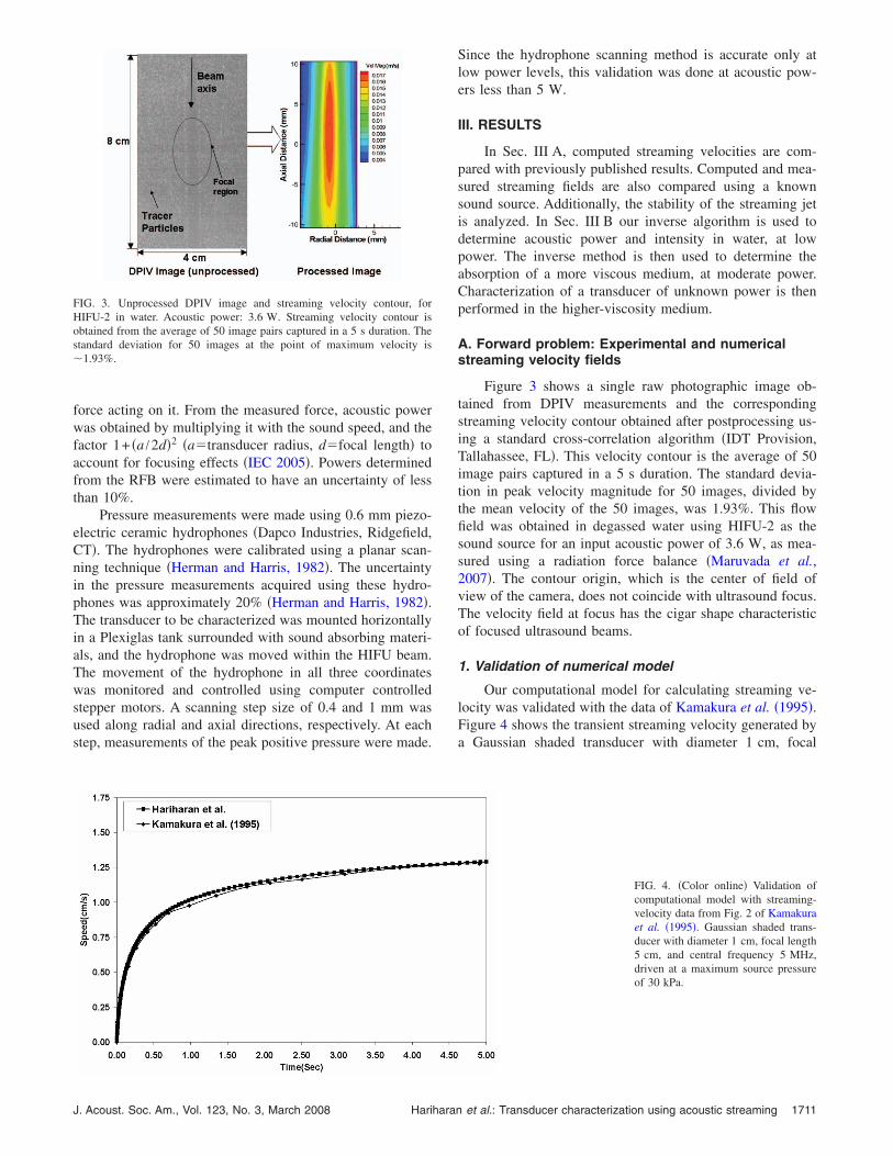
Our computational model for calculating streaming ve-locity was validated with the data of Kamakura et al. �1995�.Figure 4 shows the transient streaming velocity generated bya Gaussian shaded transducer with diameter 1 cm, focal

FIG. 3. Unprocessed DPIV image and streaming velocity contour, forHIFU-2 in water. Acoustic power: 3.6 W. Streaming velocity contour isobtained from the average of 50 image pairs captured in a 5 s duration. Thestandard deviation for 50 images at the point of maximum velocity is�1.93%.

FIG. 4. �Color online� Validation ofcomputational model with streaming-velocity data from Fig. 2 of Kamakuraet al. �1995�. Gaussian shaded trans-ducer with diameter 1 cm, focal length5 cm, and central frequency 5 MHz,driven at a maximum source pressureof 30 kPa.


length 5 cm, and central frequency 5 MHz, driven at a maxi-mum source pressure of 30 kPa. The transient speed calcu-lated using the present model matches with the result pub-lished by Kamakura et al. �Fig. 2 of Kamakura et al., 1995�to within about 1%.

2. Comparison of experimental and numericalstreaming fields

Figure 5�a� compares the radial speed profiles obtainedexperimentally using DPIV, and computationally by solvingEqs. �6�–�8� �highest and lowest curves in Fig. 5�a�, middlecurve containing “averaged data” will be discussed subse-quently�. The sound source used for this validation experi-ment is the HIFU-2 transducer �Table I�, driven at a knownacoustic power of 5.4 W, as measured using the RFB. Thepeak velocity profile calculated from the computationalmodel is �15% higher than the peak velocity measured us-ing the DPIV system. A similar trend is observed for othertransducers and other power levels.

The reason for this offset involves the finite thickness ofthe laser sheet. As mentioned earlier, the thickness of thelaser sheet �Fig. 2�a�� when it exits the Powell lens is around0.5–1 mm. However, as the laser passes through the flowmedium, the sheet diverges gradually and becomes �2 mmthick when it reaches the ultrasound beam axis �Fig. 5�b��.Therefore, instead of visualizing a single plane �2�2 cm�,the CCD camera captures particle motion in a three-

dimensional space of size 2�2�0.2 cm. As a result, thestreaming velocity measured at a particular point in the YZplane �Fig. 2�a�� is essentially the spatial average of the ve-locity occurring along the thickness of 0.2 cm of the sheet inthe x direction.

In order to account for this measurement error in ournumerical algorithm, the velocity field obtained numericallywas averaged over the 0.2 cm thickness of the laser sheet inthe x direction �Fig. 5�b��:

uaveraged =1

L�

0

L

u�r,z�dx, r = x2 + y2, �10�

where u is the velocity estimated from the computations andL is the half thickness of the laser sheet ��1 mm�. Thisaveraged velocity, uaveraged, was then used in the optimizationroutine to compute Errorrms in Eq. �9�. Figure 5 �middlecurve� shows the velocity profile calculated from our com-putations after doing the spatial averaging. The averaged ve-locity profile more closely matches the experimental data;the difference is approximately 6%.

3. Higher-viscosity streaming medium

DPIV experiments performed in water at higher acousticpowers �5–30 W� revealed the onset of instability in thestreaming jet. This instability was manifested in the form ofsmall puffs occurring at irregular times, just below the focus.This behavior was observed for all three HIFU transducers.As a result of the behavior, unrepeatable velocity fields wereobtained.

To overcome the stability problem, the viscosity of themedium was increased �Reynolds number decreased�. An al-ternative fluid medium composed of degassed water mixedwith Natrosol-L �Hydroxy ethyl cellulose, Hercules, Wilm-ington, DE� in various concentrations was developed, andused in experiments where the acoustic power exceeded5 W. The mixture was degassed using a vacuum pump priorto sonication. The viscosities of 1.4% �1.4 g /100 ml water�,2.4% and 3.4% Natrosol-L solutions were measured using aCannon type-E viscometer to be �5, �12, and �25 cp, re-spectively. Speed of sound for the 2.4% Natrosol solutionwas measured using an ultrasonic time delayed spectrometrysystem �Harris et al., 2004� to be 1480 m /s �same as fordegassed water�. Finally, as discussed in Sec. III B, the at-tenuation coefficient of the 2.4% Natrosol solution wasfound using our streaming method to be roughly twice thatof water.

Figure 6 shows radial speed profiles obtained using wa-ter as well as 1.4%, 2.4%, and 3.4% Natrosol solutions as theflow medium. The transducer used in this comparison studyis HIFU-1 excited at an output power of 30 W. Broader,smoother, and more axisymmetric profiles can be seen withincreasing Natrosol content. As the fluid viscosity increasesfrom 1 �water� to 25 cp, the peak velocity reduces from 8.2to 5.8 cm /s.

Figure 7 shows the fluid speed obtained in a 2.4% Na-trosol solution for three different transducers driven at samevoltage �42 Vrms�. The plot shows that the velocity distribu-tion at the focal region depends upon the focusing character-istics of the transducer. Focusing gain, 3, and 6 dB beam

FIG. 5. �a� Radial plot of streaming velocity in water. Transducer is HIFU-2;power5.4 W. �b� Photograph of the experimental apparatus showing thethickness of the laser sheet.


dimensions �measured from hydrophone scans� of the trans-ducers are listed in Table II. The focusing gain �Lee, 1993�,given by the expression a2

2c0d � being the central frequencyof the transducer, a the transducer radius, c0 the speed ofsound in the medium, and d the focal length�, is the highestfor HIFU-1. The corresponding peak streaming velocity ismaximum for this transducer. The velocity contours forHIFU-1 are relatively narrow, in accordance with the small6 dB beam width �Table II�. In contrast, the velocity con-tours for HIFU-3 are short in axial direction, consistent withthe smaller 6 dB width in the axial direction �Table II�. Fromthe 6 dB dimensions shown in Table II, it can be seen thatfocal region of HIFU-2 is larger than HIFU-1 and HIFU-3.Consequently, velocity contours obtained using this trans-ducer are elongated.

Figure 8 compares the streaming velocity profile ob-tained numerically and experimentally while driving HIFU-3at an input voltage of 35 Vrms, in a 12 cp medium. The cor-responding acoustic power measured using the RFB is 19 W.It can be seen that experimental and numerical velocity pro-files match closely ��1% � in both the axial and radial direc-tions.

The width of the velocity distribution in Fig. 8�b�, basedupon the distances at which the speed has dropped to half itsmaximum value �kinetic energy reduced to 1

4 the maximum�,is around 0.5 cm. By contrast, the intensity width for thesame transducer �HIFU-3� is about 0.2 cm �Table II�. In gen-eral, the width of the velocity distribution is larger than thatof the intensity distribution, and the effect becomes morepronounced as the viscosity of the medium increases. In Fig.6, for example, the width of the velocity profile for HIFU-1in the 2.4% Natrosol solution �viscosity 12 cp� is about5.4 mm. The width of the velocity profile in water �viscosity1 cp� is between 2.4 and 3.3 mm, depending upon how theasymmetry is treated. Within the limits of linear acoustics,the width of the intensity distribution is independent of vis-cosity, with the value of about 1.7 mm for HIFU-1.

B. Inverse problem: Total acoustic power and HIFUbeam characteristics

In the following, the optimization algorithm is used tobackcalculate various parameters characterizing the trans-ducer and the propagation medium.

FIG. 6. �Color online� Velocity magni-tude vs radial distance for �i� water,�ii� 1.4% Natrosol solution, �iii� 2.4%Natrosol solution, and �iv� 3.4% Na-trosol solution.

FIG. 7. Speed contours obtained in 2.4% Natrosol solution for �i� HIFU-1, �ii� HIFU-2, and �iii� HIFU-3 transducers. Transducer input voltage42 Vrms.


1. Characterizing acoustic field at low power levels„<5 W…

Since current field hydrophone mapping techniques arepractical only at low power levels, characterization was firstperformed at low input voltages with water as the fluid me-dium. Figure 9 compares the source pressure �p0

=W�2�0c0 /�a2, p0 being the peak source pressure inN /m2, W being the acoustic power in watts, and a the trans-ducer radius in m� obtained using RFB and streaming back-calculation methods. Using the procedure outlined in Fig. 1

and discussed in Sec. II, acoustic power was calculated fromthe streaming velocity for driving voltages of 15 and 18 Vrms.The source pressure of HIFU-2 was 0.048 and 0.058 MPafor driving voltages of 15 and 18 Vrms, respectively. Theinverse method predicted the source pressure to be 0.046 and0.056 MPa, which is within 5% of the values obtained fromthe RFB measurements. When the averaging prescribed byEq. �10� is not done, this deviation was �10%.

Figure 10 compares the axial and radial intensity fieldsof HIFU-2, obtained via hydrophone scanning and the in-verse method for a transducer voltage of 10 Vrms. Peak inten-sity at the focus measured by the inverse method is65 W /cm2, approximately 4% below the peak intensity mea-sured by hydrophone �67.8 W /cm2�. The 6 dB length andwidth, backcalculated from the streaming velocities, are2.7 cm�2.7 mm; the corresponding values obtained fromhydrophone scanning are 2.95 cm�3 mm.

2. Characterizing acoustic field at moderate powerlevels „<30 W…

As noted earlier, a Natrosol-based solution is the pre-ferred medium for characterization when the acoustic powerexceeds about 5 W. However, unlike water, little is knownregarding the absorption properties of Natrosol solutions.Equation �5� shows that the Reynolds stress, which accountsfor momentum transfer from the sound field to fluid, is pro-portional to the absorption coefficient of the medium. Usinga transducer of known intensity, this parameter can be treatedas the unknown in the optimization algorithm, in the follow-ing manner.

Figure 11�a� summarizes the procedure for calculatingthe acoustic absorption coefficient of the medium. UsingDPIV, the streaming velocity generated by the HIFU-2 trans-ducer in the 2.4% Natrosol-L solution was measured. First,an initial guess for the unknown � was made. In these deter-minations of absorption coefficient using the inverse algo-rithm, the attenuation coefficient of water �2.52�10−4 Np cm−1 MHz−2� was taken as the first guess for �.Then, the forcing term was calculated using Eq. �5� and thestreaming velocity was calculated numerically by solvingEqs. �6�–�8�. The Errorrms value was then computed from theexperiment and numerical velocity profiles and input into theoptimization routine. The procedure was repeated until therelative error was reduced to a value of 10−3.

The absorption coefficient of 2.4% Natrosol measuredusing this procedure is shown in Fig. 11�b�. The � valuesmeasured at the power levels 3.6, 5.8, and 11.8 W werefairly constant, approximately 5.65�10−4 Np /cm for the1.1 MHz frequency considered. This value of � is used in thesubsequent calculations to characterize transducer output atmoderate and high power/intensity levels.

Figure 12 compares the power measurements made us-ing the RFB and streaming in the 2.4% Natrosol medium.Transducers HIFU-1 and HIFU-3 were driven at voltagesranging from 19 Vrms to 42 Vrms. The inverse method wasable to measure the acoustic power with a maximum error ofabout 10%. Computed intensity profiles in the Natrosol me-dium are shown in Fig. 13, for a power of 30 W. The 6 dBlength and width, backcalculated from the streaming veloci-

TABLE II. Focusing characteristics of HIFU transducers used in the experi-ments.

Transducer 6 dB dimension �axial� radial� Focusing gain

HIFU-1 2.4 cm�1.7 mm 53HIFU-2 2.95 cm�3 mm 31HIFU-3 1.35 cm�2 mm 38

FIG. 8. �Color online� Velocity profiles obtained from computations andexperiments in 2.4% Natrosol solution; �a� velocity profile along axial di-rection and �b� velocity profile along radial direction. Transducer is HIFU-3;input voltage35 Vrms �19 W�. For the experimental data, standard devia-tion error bars for five trials are also shown. The maximum standard devia-tion for five trials is 0.02 cm /s.


ties, are 1.2 cm�1.85 mm. The values determined using hy-drophone scanning at low power, both in water and Natrosol,are 1.35 cm�2 mm �Table II�.

IV. DISCUSSION

The streaming technique as presented in this paper isuseful for characterizing HIFU transducers in the “moderate”intensity regime, roughly 100 to 1000 W /cm2. The intensi-ties are low enough that linear acoustic propagation is a rea-sonable assumption, yet high enough to possibly damageconventional hydrophones.

At low powers—around 3 W or 70 W /cm2 focal inten-sity, close agreement with piezoceramic hydrophones �Fig.10� was obtained. At focal intensities above about1000 W /cm2 �transducer powers around 20 W�, divergencebetween the measured and predicted power levels can beseen �Fig. 12�, probably due to nonlinear propagation effects.While the KZK equation can predict the generation of addi-tional frequency components by nonlinear mechanisms, theabsorption model used in our iterative method does not ac-count for the frequency dependence of the absorption. Amore comprehensive model of the absorbed acoustic energywould involve a sum of the form ��nIn, where In is theintensity of the nth acoustic harmonic and �n the correspond-ing absorption. The iterative scheme would then involve op-timization over an n-dimensional space containing the inten-sity modes. These nonlinear-propagation effects will betreated in a future generation of the model.

The inverse method was first used to determine un-known transducer power. Because we employed the linear-ized version of the KZK equation, the intensity field is lin-early proportional to the transducer power, and the KZKequation actually needed to be solved only once. Subsequentintensity fields required in the iteration process �iteration isstill required due to the more complex dependence of veloc-ity upon intensity in the Navier-Stokes equations� could beobtained by simply multiplying the first intensity field by ascaling factor dependent upon the current value of the acous-tic power. This would not be true for other transducer-

characterization parameters, such as focal length, beam tiltangle relative to the desired axis, or the absorption of themedium.

Determining an unknown absorption �Fig. 11� is a char-acterization problem for which the streaming technique iswell suited. Conventional absorption-measurement tech-niques such as time delay spectroscopy �Peters and Petit,2003� measure attenuation over a prescribed propagation dis-tance. When the attenuation is small over the given distance,these techniques are susceptible to large error. With thestreaming-based technique, however, even slight attenuationssuch as that of water can yield readily measurable fluid ve-locities. Mathematically, the forcing term in the momentumequation �Eq. �5�� contains a factor of �, producing relativechanges in the fluid velocity field that are commensuratewith relative changes in the absorption coefficient. This com-mensurate change in velocity with variation in � also allowsfor stable operation of the optimization algorithm; nonu-niqueness issues arise when the streaming field is insensitiveto changes in the parameters being determined.

The optimization technique may be used to estimatemultiple parameters simultaneously, though the computationtime increases significantly, and convergence can be moredifficult to achieve. For example, determining the transducerintensity simultaneously with the absorption coefficientwould be difficult, since the two quantities � and I0 appearprimarily as a product �Eq. �5��. The absorption coefficientalso appears in the exponential attenuating factor of the in-tensity but, as is the case with conventional absorption mea-surement techniques, this exponential factor is relatively in-sensitive to changes in �.

The streaming algorithm in this paper assumes an axi-symmetric ultrasound beam. The technique can be extendedto three-dimensional �x ,y ,z�, nonsymmetric beams with nochange in the procedures performed �Fig. 1� in the algorithm.A three-dimensional propagation code and fluid-flow simula-tor would be necessary, and an increase in computation timewould result. The three-dimensional version of the techniquewould be useful in diagnosing imperfections or problems intransducer fabrication, such as a misfiring array element or apropagation axis that was skewed relative to the axis of sym-

FIG. 9. Comparison of source pres-sure for HIFU-2 in water, obtained viathe streaming method and by radiationforce balance. Results based upon thestreaming technique are shown withand without averaging over the 2 mmlaser sheet thickness. Standard devia-tion error bars for three trials are alsoshown. For RFB measurements, themaximum standard deviation for threetrials is less than 1% of the meanvalue. For the streaming measure-ments, the maximum standard devia-tion for three trials is 3% of the mean.


metry of the transducer face. The problem would first bemanifested in an asymmetry of the experimental streamingvelocity field. The three-dimensional inverse algorithm couldbe used to help predict the transducer characteristics givingrise to the asymmetric velocity field that was observed. Forexample, the location of a nonfunctioning array elementcould be left as a free parameter in the optimization proce-dure, to be determined as part of the iterative solution.

Figure 6 illustrates the complex dependence of velocityupon fluid viscosity in a streaming medium. An increase inviscosity increases acoustic absorption, i.e., produces a largertransfer of momentum from the acoustic field to the hydro-dynamic field, resulting in a higher peak �on-axis� velocity.However, the higher viscosity also serves to radially diffusemomentum, resulting in a lower peak velocity. Thus, thepeak velocity in Fig. 6 is essentially unchanged as the vis-cosity is increased by a factor of 5 from 1 to 5 cp, but dropsabout 25% when the viscosity is doubled from 12 to 25 cp.

The higher viscosity test fluids are essential at higherstreaming velocities �higher intensities� due to stability re-quirements for the streaming jet. The higher viscosity testfluids also yield more symmetric velocity profiles, as can beseen by comparing the natrosol-based curves in Fig. 6 withthat for water. An upper limit on the viscosity of the test fluidis imposed by the low resulting velocities resulting at highviscosities. These velocities can become difficult to quantifyaccurately using DPIV systems. For the intensity range con-sidered in our studies, the agreement between experimentaland computational velocity profiles was best for the 12 cpfluid �Fig. 8�.

The KZK equation was used in our simulations, how-ever, any beam propagation code can be used in the iterativealgorithm outlined in Fig. 1. As noted by Tjotta and Tjotta�1993�, the accuracy of the KZK degrades when the beambecomes highly focused �large aperature transducers�. Tjottaand Tjotta �1993� noted that the ratio a /d of transducer ra-

FIG. 10. �Color online� Acoustic in-tensity profiles as a function of �a�axial and �b� radial distances �cm�, ob-tained from backcalculation and hy-drophone scanning in water forHIFU-2 transducer. Transducer inputvoltage10 Vrms �3.2 W�.


dius to focal length should be small in order to ensure accu-racy of the KZK approach. For our transducers HIFU-1,HIFU-2, and HIFU-3, the a /d values were 0.33, 0.35, and

0.51, respectively. While the a /d value for HIFU-3 was rela-tively large, the agreement with experimental measurementsof streaming velocity �Fig. 8� and total power �Fig. 12� indi-

FIG. 11. �Color online� �a� Flow chartof the inverse problem to estimateacoustic absorption coefficient, � �Np/cm�, of the 2.4% Natrosol fluid me-dium. �b� Absorption coefficient of2.4% Natrosol fluid obtained using theinverse method, for different powersusing HIFU-2 transducer. Standard de-viation error bars for three trials arealso shown. The maximum standarddeviation for three trials is less than1% of the mean.

FIG. 12. �Color online� Comparisonof acoustic power obtained from back-calculation and RFB in 2.4% Natrosolmedium, for transducers HIFU-1 andHIFU-3.


cates that the criterion of Tjotta may be conservative. In anyevent, when high accuracy is required, a full-wave modelsuch as the Helmholtz equation in the linear propagationregime or the Westervelt equation in the nonlinear regimeshould be employed in the iterative algorithm. The tradeoff isthe increase in computation time associated with using a full-wave model compared to a parabolic equation.

A limitation of our inverse methodology is that the re-petitive solution of the acoustic propagation equation andfluid-flow equations can involve significant computationtime ��3 h�. Our technique is also limited by the accuracy ofthe sound propagation code. For example, the KZK codecurrently employed by our model degrades in accuracy whenthe transducer gain becomes large. The above-mentioneddrawbacks can be circumvented by developing an alternatemethod which determines the acoustic field directly from theexperimental streaming velocity. In subsequent studies, anattempt will be made to estimate the acoustic field directlyfrom the experimental streaming velocity data.

V. CONCLUSION

The streaming technique presented in this paper allowsfree-field characterization of HIFU transducers to be per-formed in an intensity range that may be hazardous to con-ventional hydrophones. The method is noninvasive andagrees well with hydrophone and radiation-force balancetechniques in common ranges of applicability. In addition topredicting acoustic intensity fields, the approach may also beused to determine other important HIFU parameters, such asmedium absorption, transducer focal length, or beam tiltangle.

ACKNOWLEDGMENTS

The mention of commercial products, their sources, ortheir use in connection with material reported herein is not tobe construed as either an actual or implied endorsement ofsuch products by the U. S. Department of Health and Human

FIG. 13. �Color online� Acoustic intensity as a function of �a� axial and �b� radial distances obtained using HIFU-3 transducer in 2.4% Natrosol solution.Acoustic power30 W.


Services. Financial support from the FDA Center for Deviceand Radiological Health and the National Science Founda-tion �Grant No. 0552036� is gratefully acknowledged.

Choi, M. J., Doh, D. H., Kang, K. S., Paeng, D. G., Ko, N. H., Kim, K. S.,Rim, G. H., and Coleman, A. J. �2004�. “Visualization of acoustic stream-ing produced by lithotripsy field using a PIV method,” J. Phys.: Conf. Ser.1, 217–223.

Doinikov, A. A. �1994�. “Acoustic radiation pressure on a rigid sphere in aviscous fluid,” Proc. R. Soc. London, Ser. A 447, 447–466.

Eckart, C. �1948�. “Vortices and streams caused by sound waves,” Phys.Rev. 73, 68–76.

Fluent Inc. �2002�. FIDAP User Manual ver. 8.6.2 �Fluent, Inc., Lebanon,NH�.

Hamilton, M. F., and Morfey, C. L. �1998�. “Model equations,” in NonlinearAcoustics, edited by M. F. Hamilton and D. T. Blackstock �Academic,New York�, Chap. 3.

Hariharan, P., Banerjee, R. K., and Myers, M. R. �2007�. “HIFU proceduresat moderate intensities: Effect of large blood vessels,” Phys. Med. Biol.52, 3493–3513.

Harland, A. R., Petzing, J. N., and Tyrer, J. R. �2002�. “Non-invasive mea-surements of underwater pressure fields using laser Doppler velocimetry,”J. Sound Vib. 252, 169–177.

Harris, G. R. �2005�. “Progress in medical ultrasound exposimetry,” IEEETrans. Ultrason. Ferroelectr. Freq. Control 52, 717–736.

Harris, G. R., Gammell, P. M., Lewin, P. A., and Radulescu, E. �2004�.“Interlaboratory evaluation of hydrophone sensitivity calibration from0.1 MHz to 2 MHz via time delay spectrometry,” Ultrasonics 42, 349–353.

Hartley, C. J. �1997�. “Characteristics of acoustic streaming created andmeasured by pulsed Doppler ultrasound,” IEEE Trans. Ultrason. Ferro-electr. Freq. Control 44, 1278–1285.

Herman, B., and Harris, G. R. �1982�. “Calibration of miniature ultrasonictransducers using a planar scanning technique,” J. Acoust. Soc. Am. 72,1357–1362.

International Electrotechnical Commission �IEC�. �2005�. “Powermeasurement—Radiation force balances and performance requirements upto 1 W in the frequency range 0.5 MHz to 25 MHz and up to 20 W in thefrequency range 0.75 MHz and 5 MHz,” Ultrasonics 87, 1–44.

Kamakura, T., Kazuhisa, M., Kumamoto, Y., and Breazeale, M. A. �1995�.“Acoustic streaming induced in focused Gaussian beams,” J. Acoust. Soc.Am. 97, 2740–2746.

King, L. V. �1934�. “On the acoustic radiation pressure on spheres,” Proc. R.Soc. London, Ser. A 147, 212–240.

Lagarias, J. C., Reeds, J. A., Wright, M. H., and Wright, P. E. �1995�.“Convergence properties of the Nelder-Mead algorithm in low dimen-sions,” AT&T Bell Laboratories, Technical Report, Murray Hill, NJ.

Lee, Y. S. �1993�. “Numerical solution of the KZK equation for pulsed finiteamplitude sound beams in thermoviscous fluids,” Ph.D. dissertation, Uni-versity of Texas at Austin, Austin, TX.

Lighthill, J. �1978a�. “Acoustic streaming,” J. Sound Vib. 61, 391–418.Lighthill, J. �1978b�. Waves in Fluids �Cambridge University Press, Cam-

bridge, U.K�.

Madelin, G., Grucker, D., Franconi, J. M., and Thiaudiere, E. �2006�. “Mag-netic resonance imaging of acoustic streaming: Absorption coefficient andacoustic field shape estimation,” Ultrasonics 44, 272–278.

Maruvada, S., Harris, G. R., Herman, B. A., and King, R. L. �2007�.“Acoustic power calibration of high-intensity focused ultrasound transduc-ers using a radiation force technique,” J. Acoust. Soc. Am. 121, 1434–1439.

Mathworks Inc. �2002�. Matlab Manual �Mathworks, Inc., Natick, MA�, ver.6.5.

Morse, P. M., and Ingard, K. U. �1968�. Theoretical Acoustics �McGraw-Hill, New York�.

Nowicki, A., Kowalewski, T., Secomski, W., and Wojcik, J. �1998�. “Esti-mation of acoustical streaming: Theoretical model, Doppler measurementsand optical visualization,” Eur. J. Ultrasound 7, 73–81.

Nyborg, W. L. �1965�. Physical Acoustics �Academic, New York�, Vol 2B.Peters, F., and Petit, L. �2003�. “A broad band spectroscopy method for

ultrasound wave velocity and attenuation measurement in dispersive me-dia,” Ultrasonics 41, 357–363.

Prasad, A. K. �2000�. “Particle image velocimetry,” Eur. Trans Telecommun.Relat. Technol. 79, 51–60.

Robinson, R. A., and Ilev, I. K. �2004�. “Design and optimization of aflexible high-peak-power laser-to-fiber coupled illumination system usedin digital particle image velocimetry,” Rev. Sci. Instrum. 75, 4856–4863.

Schafer, M. E., Gessert, J. E., and Moore, W. �2006�. “Development of ahigh intensity focused ultrasound �HIFU� hydrophone system,” Proc. Int.Symp. Therapeutic Ultrasound 829, 609–613.

Shaw, A. �2004�. “Delivering the right dose, advanced metrology for ultra-sound in medicine,” J. Phys.: Conf. Ser. 1, 174–179.

Shaw, A., and ter Haar, G. R. �2006�. “Requirements for measurement stan-dards in high intensity focused �HIFU� ultrasound fields,” National Physi-cal Laboratory �NPL� Report, ISSN 1744-0599.

Shi, X., Martin, R. W., Vaezy, S., and Crum, L. A. �2002�. “Quantitativeestimation of acoustic streaming in blood,” J. Acoust. Soc. Am. 111, 1110–1121.

Starritt, H. C., Duck, F. A., and Humphrey, V. F. �1989�. “An experimentalinvestigation of streaming in pulsed diagnostic ultrasound beams,” Ultra-sound Med. Biol. 15, 363–373.

Starritt, H. C., Duck, F. A., and Humphrey, V. F. �1991�. “Force acting in thedirection of propagation in pulsed ultrasound fields,” Phys. Med. Biol. 36,1465–1474.

Theobald, P., Thompson, A., Robinson, S., Preston, R., Lepper, P., Swift, C.,Yuebing, W., and Tyrer, J. �2004�. “Fundamental standards for acousticsbased on optical methods–Phase three report for sound in water,” ReportNo. CAIR9 ISSN 1740-0953, National Physical Laboratory �NPL�, Ted-dington, England.

Tjotta, S., and Tjotta, N. J. �1993�. “Acoustic streaming in ultrasoundbeams,” in Advances in Nonlinear Acoustics, 13th International Sympo-sium on Nonlinear Acoustics, edited by H. Hobaek �World Scientific, Sin-gapore�, pp. 601–606.

Wang, Z. Q., Lauxmann, P., Wurster, C., Kohler, M., Gompf, B., and Eisen-menger, W. �1999�. “Impulse response of a fiber optic hydrophone deter-mined with shock waves in water,” J. Appl. Phys. 85, 2514–2516.

Zanelli, C. I., and Howard, S. M. �2006�. “A robust hydrophone for HIFUMetrology,” Proc. Int. Symp. Therapeutic Ultrasound 829, 618–622.


characterization of high intensity focused ultrasound ... of high intensity focused ultrasound...

Documents