characterization of a variable diameter bioreactor (vdb) by
TRANSCRIPT
i
Characterization of a Variable Diameter Bioreactor (VDB)
BY
ZHE SU
B.S., Liaoning Shihua University, 2016
Master’s Thesis
Submitted to the University of New Hampshire
in Partial Fulfillment of
the Requirements for the Degree of
Master of Science
in
Chemical Engineering
September 2020
ii
This dissertation was examined and approved in partial fulfillment of the requirements for the
degree of Master of Science in Chemical Engineering by:
Thesis Director, Dr. Kang Wu, Associate
Professor of Chemical Engineering
Dr. Young Jo Kim, Assistant Professor of
Chemical Engineering
Dr. Nan Yi, Assistant Professor of Chemical
Engineering
On July 27th, 2020
Approval signatures are on file with the University of New Hampshire Graduate School.
iii
DEDICATION
I dedicate this work with love to my parents, Qinglian Su and Meiling Huang who have
supported me throughout my education. Thanks for making me see this adventure through the
end.
iv
ACKNOWLEDGEMENTS
I would like to acknowledge my advisor with sincere gratitude and respect, Kang Wu who taught
me everything I know in molecular cloning and spore surface display system. Your generous
support over the years inspired me in countless ways academically, professionally, and
personally.
I would also like to acknowledge my other committee members, Dr. Kim and Dr. Yi. I would
like to thank Dr. Kim for teaching me everything I know about heat transfer. Also, thank you to
Dr. Yi not only for teaching me everything I know about kinetics, but also give me valuable
suggestions for the future.
I would also like to acknowledge the past and present students of the Wu lab group; Guo Wu,
Adam Rosenbaum and Griffin Kane. I could not ask for better lab mates and I wish them the best
of luck in their endeavors. A tender expression of acknowledgement and gratitude to my
girlfriend, Cuihong Song, for providing me with the grounding, good care and emotional support
that sustained me through the journey. Finally, I would like to acknowledge my parents, Qinglian
Su and Meiling Huang, for unconditionally loving me and encouraging all of my pursuits.
v
Table of Contents
ACKNOWLEDGEMENTS ................................................................................................................................. iv
LIST OF TABLES.............................................................................................................................................. vii
LIST OF FIGURES ........................................................................................................................................... viii
ABSTRACT ......................................................................................................................................................... xi
Chapter 1: Introduction ....................................................................................................................................... 1
1.1 Background of bioreactors ........................................................................................................................... 1
1.2 Types of bioreactors ..................................................................................................................................... 4 1.2.1 Continuous Stirred Tank Bioreactors (CSTR) ........................................................................................ 4 1.2.2 Bubble Column Bioreactors .................................................................................................................. 5 1.2.3 Airlift Bioreactor .................................................................................................................................. 6 1.2.4 Fluidized Bed Bioreactor ...................................................................................................................... 8 1.2.5 Packed Bed Bioreactor .......................................................................................................................... 9 1.2.6 Photo Bioreactor ................................................................................................................................. 10
1.3 Scale Up of Bioreactors.............................................................................................................................. 11
1.4 Variable Diameter Bioreactor (VDB) ......................................................................................................... 13
1.5 Objectives .................................................................................................................................................. 15
Chapter 2: Material and Method ....................................................................................................................... 16
2.1 Solution ..................................................................................................................................................... 16 2.1.1 Mixing Time....................................................................................................................................... 16 2.1.2 Mass Transfer Coefficient (kLa) .......................................................................................................... 17
2.2 Fabrication of Bioreactor ........................................................................................................................... 17 2.2.1 Fabrication and Assembly ................................................................................................................... 17 2.2.2 Assembly............................................................................................................................................ 19 2.2.3 Data Collection ................................................................................................................................... 20
2.3 Method of mixing time calculation. ............................................................................................................. 20
2.4 Method of kLa calculation. .......................................................................................................................... 20
Chapter 3: Results and Discussion ..................................................................................................................... 22
3.1 Mixing Time ............................................................................................................................................... 22 3.1.1 Determination of the Mixing Time Point ............................................................................................. 22 3.1.2 Mixing Time Results and Discussion .................................................................................................. 25
3.2 Mass Transfer Coefficient (kLa) .................................................................................................................. 45 3.2.1 Characterization of Mass Transfer Coefficient (kLa) in 100L, 40L, 20L and 5L VDB ........................... 46 3.2.2 Characterization of Mass Transfer Coefficient (kLa) in 100L and 20L Conventional Reactor with
Continuous Impeller .................................................................................................................................... 51 3.2.3 Characterization of Mass Transfer Coefficient (kLa) in 100L and 40L Conventional Reactor with
Conventional Impeller ................................................................................................................................. 54 3.2.4 Characterization of Mass Transfer Coefficient (kLa) in 100L VDB, 100L Conventional Reactor with
Continuous Impeller and 100L Conventional Reactor with Conventional Impeller. ....................................... 56
vi
3.2.5 Characterization of Mass Transfer Coefficient (kLa) in 40L VDB and 40L Conventional Reactor with
Conventional Impeller. ................................................................................................................................ 59 3.2.6 Characterization of Mass Transfer Coefficient (kLa) in 20L VDB and 20L Conventional Reactor with
Continuous Impeller. ................................................................................................................................... 61
Chapter 4: Biosynthesis of Antimicrobial Peptides (AMPs) ............................................................................. 64
4.1 Introduction ............................................................................................................................................... 64 4.1.1 Antimicrobial Peptides (AMPs) .......................................................................................................... 64 4.1.2 B. subtilis, Spores and Spore Surface Display ...................................................................................... 68 4.1.3 Intein .................................................................................................................................................. 71
4.2 Material and Method .................................................................................................................................. 72 4.2.1 Media and Solutions ........................................................................................................................... 72 4.2.2 Plasmid, Synthesized DNA and Primers .............................................................................................. 73 4.2.3 Polymerase Chain Reaction (PCR) ...................................................................................................... 75 4.2.4 Gel electrophoresis and DNA recovery................................................................................................ 76 4.2.5 DNA Concentration Measurement ...................................................................................................... 77 4.2.6 E. coli Transformation ........................................................................................................................ 77 4.2.7 B. subtilis Integration and Sporulation ................................................................................................. 78 4.2.8 SDS-PAGE......................................................................................................................................... 79
5.3 Results and Discussion ............................................................................................................................... 80 5.3.1 Plasmids Construction ........................................................................................................................ 80 5.3.2 Sporulation ......................................................................................................................................... 84
LIST OF REFERENCE ..................................................................................................................................... 86
vii
LIST OF TABLES
Table 3- 1 Mixing for conventional reactor with continuous impeller, 40L, 180 agitation, 16704
mL/min airflow rate. ................................................................................................................. 22
Table 3- 2 Parameters for characterization of mixing time in 100L prototypes. .......................... 26
Table 3- 3 Parameters for characterization of mass transfer coefficient (kLa) in 100L prototypes.
................................................................................................................................................. 46
Table 4- 1 Plasmids used in this study ....................................................................................... 73
Table 4- 2 Synthesized Gene Sequences .................................................................................... 74
Table 4- 3 Primers used in this work. ........................................................................................ 75
Table 4- 4 PCR Reaction Solutions for GoTaq Green Master Mix and LongAmp Taq DNA
Polymerase................................................................................................................................ 75
Table 4- 5 Thermocycling Working Conditions for PCR ........................................................... 75
Table 4- 6 DNA Concentration Measurement Solutions ............................................................ 77
Table 4- 7 B. subtilis Integration Solutions ................................................................................ 78
Table 4- 8 DNA fragments amplify list ..................................................................................... 80
viii
LIST OF FIGURES
Figure 1- 1 Continuous Stirred Tank Reactor (CSTR) .................................................................5
Figure 1- 2 Bubble Column Bioreactors ......................................................................................6
Figure 1- 3 Airlift Bioreactor(Mahmood et al., 2015) ..................................................................7
Figure 1- 4 Fluidized Bed Bioreactor...........................................................................................9
Figure 1- 5 Packed Bed Bioreactor ............................................................................................ 10
Figure 1- 6 Photo Bioreactor(Chen et al., 2011)......................................................................... 11
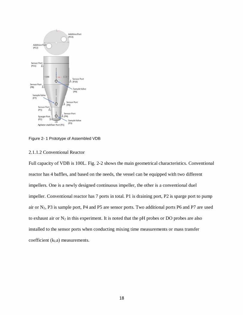
Figure 2- 1 Prototype of Assembled VDB ................................................................................. 18
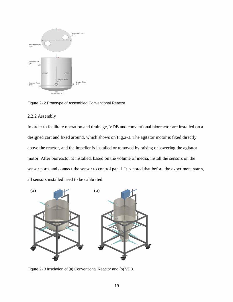
Figure 2- 2 Prototype of Assembled Conventional Reactor ........................................................ 19
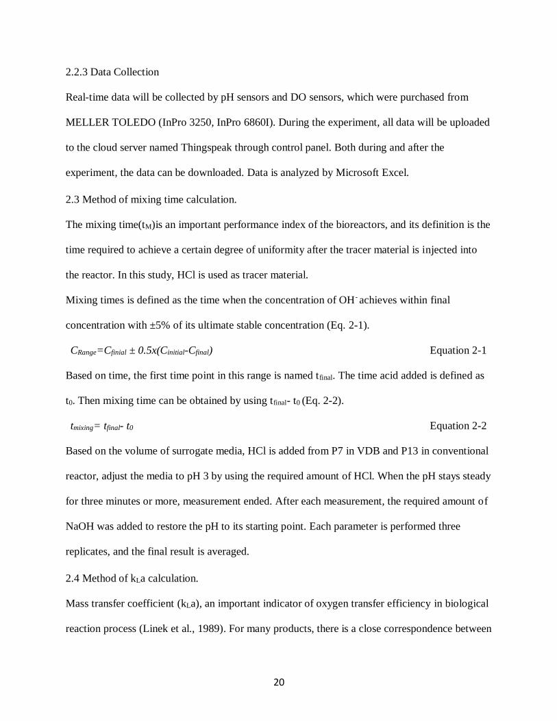
Figure 2- 3 Insolation of (a) Conventional Reactor and (b) VDB. .............................................. 19
Figure 3- 1 Mixing time for conventional reactor with continuous impeller, 40L, 150 RPM,
16704 mL/min airflow rate. ....................................................................................................... 23
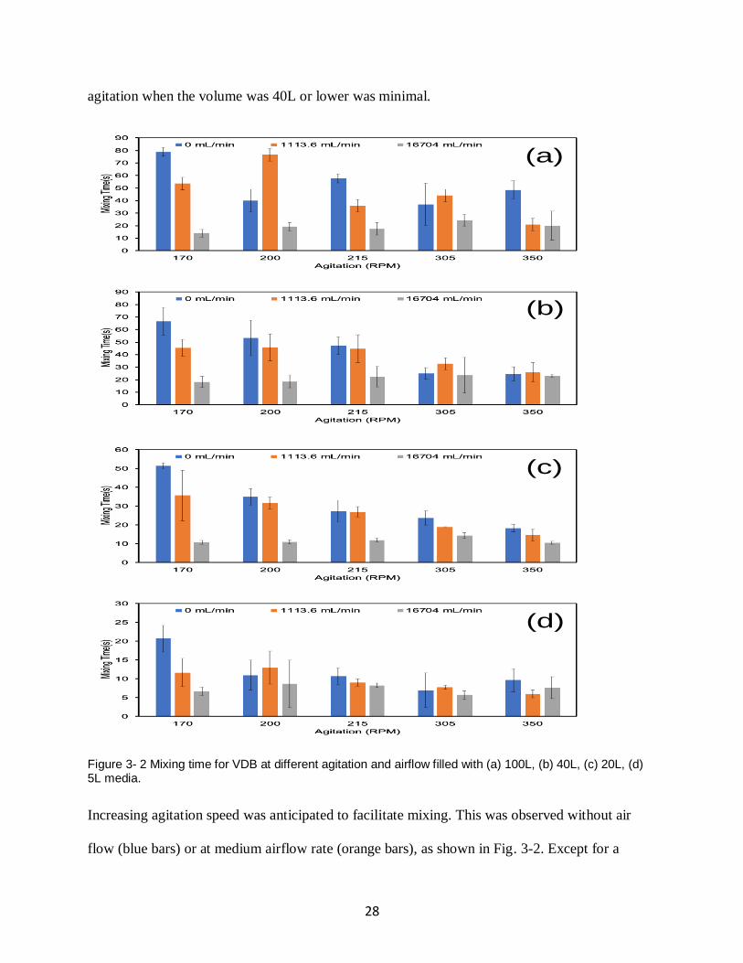
Figure 3- 2 Mixing time for VDB at different agitation and airflow filled with (a) 100L, (b) 40L,
(c) 20L, (d) 5L media. ............................................................................................................... 28
Figure 3- 3 Mixing time for VDB at different volumes and airflow in (a) 170 RPM, (b) 200
RPM, (c) 215 RPM, (d) 305 RPM, (e) 350 RPM. ...................................................................... 30
Figure 3- 4 Mixing time for conventional reactor with continuous impeller at different agitation
and airflow filled with (a) 100L, (b) 20L media. ........................................................................ 33
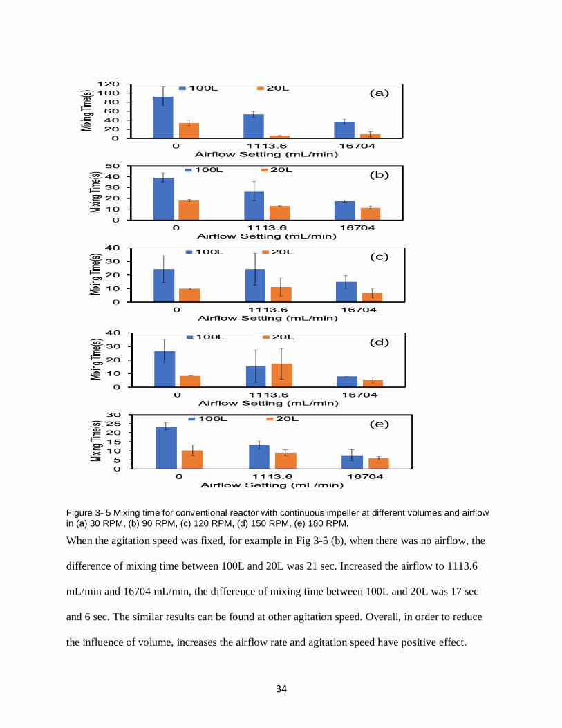
Figure 3- 5 Mixing time for conventional reactor with continuous impeller at different volumes
and airflow in (a) 30 RPM, (b) 90 RPM, (c) 120 RPM, (d) 150 RPM, (e) 180 RPM. ................. 34
Figure 3- 6 Mixing time for conventional reactor with conventional impeller at different agitation
and airflow filled with (a) 100L, (b) 40L media. ........................................................................ 36
ix
Figure 3- 7 Mixing time for conventional reactor with conventional impeller at different volumes
and airflow in (a) 30 RPM, (b) 90 RPM, (c) 120 RPM, (d) 150 RPM, (e) 180 RPM. ................. 37
Figure 3- 8 Mixing time for VDB, conventional reactor with continuous impeller and
conventional reactor with conventional impeller in 100L, (a) 0 airflow, (b) 1113.6 mL/min
airflow and (c) 16704 mL/min airflow. ...................................................................................... 40
Figure 3- 9 Mixing time for VDB and conventional reactor with conventional impeller in 40L,
(a) 0 airflow, (b) 1113.6 mL/min airflow and (c) 16704 mL/min airflow. .................................. 42
Figure 3- 10 Mixing time for VDB and conventional reactor with continuous impeller in 20L, (a)
0 airflow, (b) 1113.6 mL/min airflow and (c) 16704 mL/min airflow. ....................................... 44
Figure 3- 11 Mass transfer coefficient (kLa) for VDB at different agitation and airflow filled with
(a) 100L, (b) 40L, (c) 20L, (d) 5L media. .................................................................................. 48
Figure 3- 12 Mass transfer coefficient (kLa) for VDB at different volumes and airflow (a) 170
RPM, (b) 200 RPM, (c) 215 RPM, (d) 305 RPM, (e) 350 RPM. ................................................ 50
Figure 3- 13 Mass Transfer Coefficient (kLa) for conventional reactor with continuous impeller
at different agitation and airflow filled with (a) 100L, (b) 20L media. ....................................... 52
Figure 3- 14 Mass Transfer Coefficient (kLa) for conventional reactor with continuous impeller
at different volumes and airflow in (a) 30 RPM, (b) 90 RPM, (c) 120 RPM, (d) 150 RPM, (e)
180 RPM. .................................................................................................................................. 53
Figure 3- 15 Mass Transfer Coefficient (kLa) for conventional reactor with conventional impeller
at different agitation and airflow filled with (a) 100L, (b) 40L media. ....................................... 54
Figure 3- 16 Mass Transfer Coefficient (kLa) for conventional reactor with conventional impeller
at different volumes and airflow in (a) 30 RPM, (b) 90 RPM, (c) 120 RPM, (d) 150 RPM, (e)
180 RPM. .................................................................................................................................. 56
x
Figure 3- 17 Mass transfer coefficient (kLa) for VDB, conventional reactor with continuous
impeller and conventional reactor with conventional impeller in 100L, (a) 0 airflow, (b) 10
airflow and (c) 150 airflow. ....................................................................................................... 58
Figure 3- 18 Mass transfer coefficient (kLa) for VDB and conventional reactor with conventional
impeller in 40L, (a) 1113.6 mL/min airflow, (b) 5568 mL/min, (c) 11136 mL/min airflow and (d)
16704 mL/min airflow. ............................................................................................................. 60
Figure 3- 19 Mass transfer coefficient (kLa) for VDB and conventional reactor with continuous
impeller in 20L, (a) 0 airflow, (b) 1113.6 mL/min airflow and (c) 16704 mL/min airflow. ........ 62
Figure 4- 1 Protentional problems, a) antimicrobial peptides kill host cell, b) antimicrobial
peptides degrade in host cell by using E. coli as host cell. .......................................................... 67
Figure 4- 2 (a) B. subtilis image(Chen, R. et al., 2009) and (b) sporulation ................................ 69
Figure 4- 3 (a) Wild type spore, (b) AMPs fused with coat protein gene sequence, c) engineered
spore with AMPs on spore surface. ........................................................................................... 70
Figure 4- 4 pDG1662 Plasmid Map. .......................................................................................... 74
Figure 4- 5 Colony PCR gel image of AMP1, AMP1, AMP2, AMP2 and AMP3, AMP3 in E.
coli (top to bottom). .................................................................................................................. 81
Figure 4- 6 Colony PCR gel image of AMP4, AMP4, AMP5, AMP5 and AMP6, AMP6 in E.
coli (top to bottom). .................................................................................................................. 82
Figure 4- 7 Colony PCR gel image of AMP7, AMP8 and AMP9 in E. coli (top to bottom). ...... 83
Figure 4- 8 Plate image of positive control, negative control, AMP8 and AMP9........................ 83
Figure 4- 9 Colony PCR gel image of AMP8 colony 1, 2, 3, 4 and AMP9 colony 1, 2 in B.
Subtilis (top to bottom). ............................................................................................................. 83
Figure 4- 10 Spore image of AMP8 and AMP9 (left to right). ................................................... 84
xi
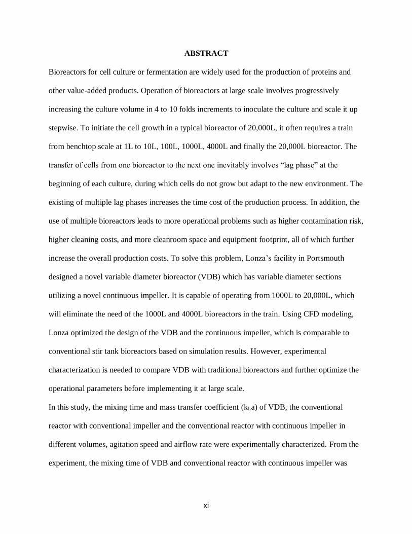
ABSTRACT
Bioreactors for cell culture or fermentation are widely used for the production of proteins and
other value-added products. Operation of bioreactors at large scale involves progressively
increasing the culture volume in 4 to 10 folds increments to inoculate the culture and scale it up
stepwise. To initiate the cell growth in a typical bioreactor of 20,000L, it often requires a train
from benchtop scale at 1L to 10L, 100L, 1000L, 4000L and finally the 20,000L bioreactor. The
transfer of cells from one bioreactor to the next one inevitably involves “lag phase” at the
beginning of each culture, during which cells do not grow but adapt to the new environment. The
existing of multiple lag phases increases the time cost of the production process. In addition, the
use of multiple bioreactors leads to more operational problems such as higher contamination risk,
higher cleaning costs, and more cleanroom space and equipment footprint, all of which further
increase the overall production costs. To solve this problem, Lonza’s facility in Portsmouth
designed a novel variable diameter bioreactor (VDB) which has variable diameter sections
utilizing a novel continuous impeller. It is capable of operating from 1000L to 20,000L, which
will eliminate the need of the 1000L and 4000L bioreactors in the train. Using CFD modeling,
Lonza optimized the design of the VDB and the continuous impeller, which is comparable to
conventional stir tank bioreactors based on simulation results. However, experimental
characterization is needed to compare VDB with traditional bioreactors and further optimize the
operational parameters before implementing it at large scale.
In this study, the mixing time and mass transfer coefficient (kLa) of VDB, the conventional
reactor with conventional impeller and the conventional reactor with continuous impeller in
different volumes, agitation speed and airflow rate were experimentally characterized. From the
experiment, the mixing time of VDB and conventional reactor with continuous impeller was
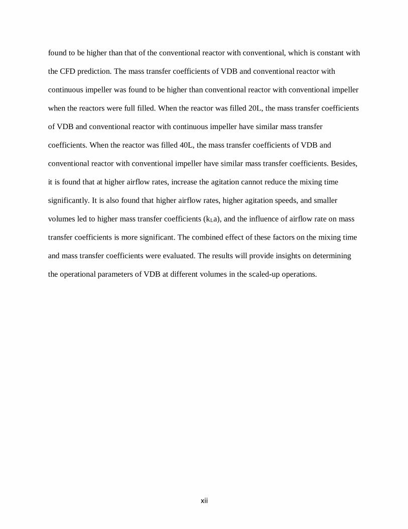
xii
found to be higher than that of the conventional reactor with conventional, which is constant with
the CFD prediction. The mass transfer coefficients of VDB and conventional reactor with
continuous impeller was found to be higher than conventional reactor with conventional impeller
when the reactors were full filled. When the reactor was filled 20L, the mass transfer coefficients
of VDB and conventional reactor with continuous impeller have similar mass transfer
coefficients. When the reactor was filled 40L, the mass transfer coefficients of VDB and
conventional reactor with conventional impeller have similar mass transfer coefficients. Besides,
it is found that at higher airflow rates, increase the agitation cannot reduce the mixing time
significantly. It is also found that higher airflow rates, higher agitation speeds, and smaller
volumes led to higher mass transfer coefficients (kLa), and the influence of airflow rate on mass
transfer coefficients is more significant. The combined effect of these factors on the mixing time
and mass transfer coefficients were evaluated. The results will provide insights on determining
the operational parameters of VDB at different volumes in the scaled-up operations.
1
Chapter 1: Introduction
1.1 Background of bioreactors
A bioreactor is a device system that uses enzymes or organisms to perform biochemical reactions
in vitro. It is a bio function simulator, such as a fermentation tank, immobilized enzyme or
immobilized cell reactor. It has essential applications in the production of alcohol, medicine,
concentrated jams, fermentation of fruit juices, and organic degradation (Van't Riet and Tramper,
1991).
Bioreactors are essential technologies for the development of the biotechnology industry.
Because the bioreactor energy consumption is not high, and the product can be produced with the
participation of enzymes and microorganisms under normal temperatures and pressures, the
production of various products through cell culture in bioreactors is an important part of the
industrialization of biotechnology in the world, involving a variety of industries, such as
medicine, chemical industry, light industry, food, agriculture, marine, environmental protection,
and other industries (Kim et al., 2002). At this stage, microorganisms and different types of cells,
such as animal cells, plant cells, and algae cells can also be cultured through biotechnology, have
gradually attracted enormous attention and have shown encouraging prospects. And with the
development of biotechnology, many biologically active substances discovered by humans in the
future can be obtained by means of cell culture methods. Through genetic engineering, genes
from different origins can be combined according to pre-designed blueprints, and then
introduced them into a host cell to change the original genetic characteristics of the organisms,
give it new properties, and/or used to produce new products (Daniell et al., 2002; Mantell et al.,
1985). These new products can be cell metabolites, enzymes, or gene expression products. Then
the company can produce the new product in a large scale through bioreactor to improve the
2
economic benefit. For example, the vitamins, erythromycin, and cinnamic we eat, penicillin,
streptomycin, and gentamicin for injection are biological products obtained by fermentation of
different microorganisms (Warnock and Al‐Rubeai, 2006). The vast majority of antibiotics used
in medicine come from microorganisms, and each product has strict production standards. Other
medicine which is used in the treatment of cancer, AIDS, coronary heart disease, anemia,
dysplasia, diabetes, and other diseases, also can be produced through fermentation in bioreactors
(Altman et al., 2002; Liu et al., 2018).
The goal of the bioreactors is to create an optimal environment where microorganisms or cells
can express their function and produce products with impurities within the standard. Therefore,
in the production process, the control of temperature, pH, oxygen solubility and other parameters
which will affect the growth of organisms and cells are important (Simutis and Lübbert, 2015).
Temperature is a critical parameter, which can influence the manufacturing process significantly.
For example, the suitable temperature for mammalian and avian cell culture is 37~38℃, low
temperature in the bioreactor may cause cells to grow slowly and even lead to the death (Lee,
1996). Therefore, controlling the temperature in the bioreactor is important. The temperature that
affects the bioreactor can be maintained by using a cooling jacket, a coil, or both (Broadley and
Benton, 2010; Nagel et al., 2001). A cooling jacket is essential for large industrial fermentation
tanks. Industrial fermentation tanks are almost always made of stainless steel. The fermentation
tank is a large cylinder with closed top and bottom, and various pipes and valves at the same
time. The fermentation tank is externally inserted with a cooling jacket, and cold or hot water is
run through the cooling jacket to achieve the purpose of temperature control. For very large
bioreactors, the heat transfer through the jacket is not enough. Therefore, an internal coil is
provided to help the cooling jacket to control the temperature. By using the cooling jacket and/or
3
coil, the temperature is controlled within a range suitable for cell growth. In addition, after the
manufacture process is completed, steam can also go through cooling jackets or coils for the
purpose of sterilization.
The control of pH is also a crucial step in the production process. In the industrial manufacturing
process, various cells have different requirements for pH in different bioreactions. Most cells are
suitable for growth under pH between 7.2 and 7.4, below pH 6.8 or above pH 7.6 is harmful to
cells, even degeneration or death (Horiuchi et al., 2003). However, during the growth of cells,
with the increase of the number of cells and the enhancement of metabolic activity, carbon
dioxide is continuously released. After carbon dioxide dissolves in the culture, it results in the
change of pH value (Fradette and Ruel, 2009). Therefore, pH sensors are used to detect the
changes of pH value. And when the pH value in the culture is not conducive to cell growth, a
small amount of acid or alkali is added to adjust the pH to the suitable value.
Oxygen is one of the essential elements for cell growth. Dissolved oxygen is detected by DO
sensors. Insufficient oxygen supply can cause cells to grow slowly or even die, especially when
the density of cells in the bioreactor is high (Lee et al., 2008). Due to the low solubility of
oxygen in water and the low oxygen content (20.95%) in the air, so air or pure oxygen must be
continuously added to the reaction system through an aeration system. Appropriately aeration
systems can ensure sufficient oxygen supply throughout the cultivation process. The aeration
system is consisted of two parts, sparger and impeller. The sparger is usually just a series of
holes in the metal ring or nozzle (Polli et al., 2002), and the impeller is a tool used to break the
bubbles and evenly distributed throughout the container (Tunac, 1991). When the air or oxygen
sterilized by the filter enters the cell culture through the high-pressure hole on sparger, the
impeller will distribute the air or oxygen throughout the bioreactor rapidly. In addition to support
4
the growth of cells, the rising bubbles in the culture can help the mixing of nutrient in
bioreactors, and also can exhaust the waste gas, such as carbon dioxide. Therefore, the oxygen
supply not only maintains the growth of the cells, but also maintains the condition of the culture
medium.
In addition, the agitation speed of the impeller in reactor is also very important. If the agitation
speed is slow, the cells tend to clump, sink and adhere, which is not conducive to the growth of
cells. If the agitation speed is high, the culture will foam, and the cells will suffocate to death
(Kunas and Papoutsakis, 1990). Besides, vigorous agitation can cause cells to rupture due to
mechanical damage. Therefore, it is important to choose a suitable stirring speed.
1.2 Types of bioreactors
The following six types of bioreactors are commonly used in biotechnology (Asenjo, 1994; Spier
et al., 2011). They are (1) Continuous Stirred Tank Bioreactors (2) Bubble Column Bioreactors
(3) Airlift Bioreactors (4) Fluidized Bed Bioreactors (5) Packed Bed Bioreactors and (6) Photo-
Bioreactors.
1.2.1 Continuous Stirred Tank Bioreactors (CSTR)
A continuous stirred tank reactor (CSTR) refers to a tank reactor with a stirring paddle. The
structure of the CSTR reactors are shown in Figure 1-1. The purpose of stirring is to make the
material system reach a uniform state, which is beneficial to the reaction and heat transfer
uniformity. The reaction process includes the physical and chemical changes of the materials in
the system, and the parameters characterized in the system include temperature, pressure, liquid
level, and system components (Trambouze and Piret, 1959). The purpose of the reactor's reaction
is to complete the fermentation of feed liquid and produce biogas in a closed tank (Boe and
Angelidaki, 2009). Because the stirring device is installed in the reactor, the fermentation raw
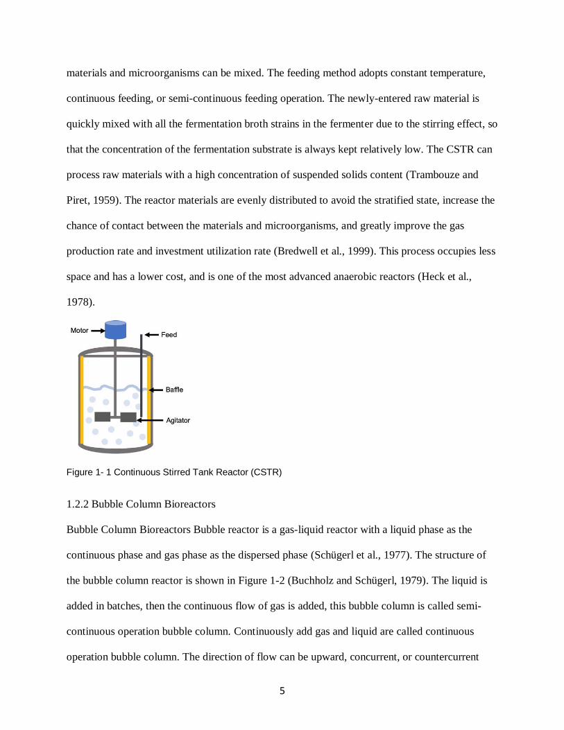
5
materials and microorganisms can be mixed. The feeding method adopts constant temperature,
continuous feeding, or semi-continuous feeding operation. The newly-entered raw material is
quickly mixed with all the fermentation broth strains in the fermenter due to the stirring effect, so
that the concentration of the fermentation substrate is always kept relatively low. The CSTR can
process raw materials with a high concentration of suspended solids content (Trambouze and
Piret, 1959). The reactor materials are evenly distributed to avoid the stratified state, increase the
chance of contact between the materials and microorganisms, and greatly improve the gas
production rate and investment utilization rate (Bredwell et al., 1999). This process occupies less
space and has a lower cost, and is one of the most advanced anaerobic reactors (Heck et al.,
1978).
Figure 1- 1 Continuous Stirred Tank Reactor (CSTR)
1.2.2 Bubble Column Bioreactors
Bubble Column Bioreactors Bubble reactor is a gas-liquid reactor with a liquid phase as the
continuous phase and gas phase as the dispersed phase (Schügerl et al., 1977). The structure of
the bubble column reactor is shown in Figure 1-2 (Buchholz and Schügerl, 1979). The liquid is
added in batches, then the continuous flow of gas is added, this bubble column is called semi-
continuous operation bubble column. Continuously add gas and liquid are called continuous
operation bubble column. The direction of flow can be upward, concurrent, or countercurrent
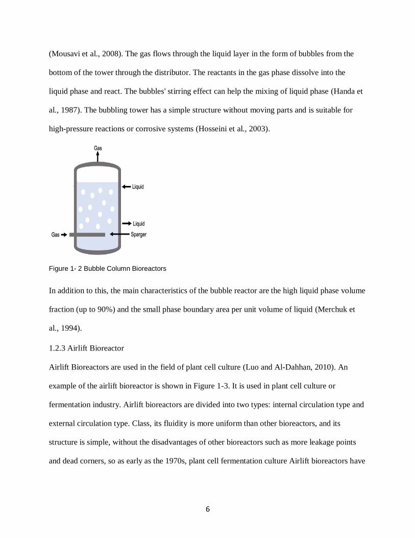
6
(Mousavi et al., 2008). The gas flows through the liquid layer in the form of bubbles from the
bottom of the tower through the distributor. The reactants in the gas phase dissolve into the
liquid phase and react. The bubbles' stirring effect can help the mixing of liquid phase (Handa et
al., 1987). The bubbling tower has a simple structure without moving parts and is suitable for
high-pressure reactions or corrosive systems (Hosseini et al., 2003).
Figure 1- 2 Bubble Column Bioreactors
In addition to this, the main characteristics of the bubble reactor are the high liquid phase volume
fraction (up to 90%) and the small phase boundary area per unit volume of liquid (Merchuk et
al., 1994).
1.2.3 Airlift Bioreactor
Airlift Bioreactors are used in the field of plant cell culture (Luo and Al-Dahhan, 2010). An
example of the airlift bioreactor is shown in Figure 1-3. It is used in plant cell culture or
fermentation industry. Airlift bioreactors are divided into two types: internal circulation type and
external circulation type. Class, its fluidity is more uniform than other bioreactors, and its
structure is simple, without the disadvantages of other bioreactors such as more leakage points
and dead corners, so as early as the 1970s, plant cell fermentation culture Airlift bioreactors have
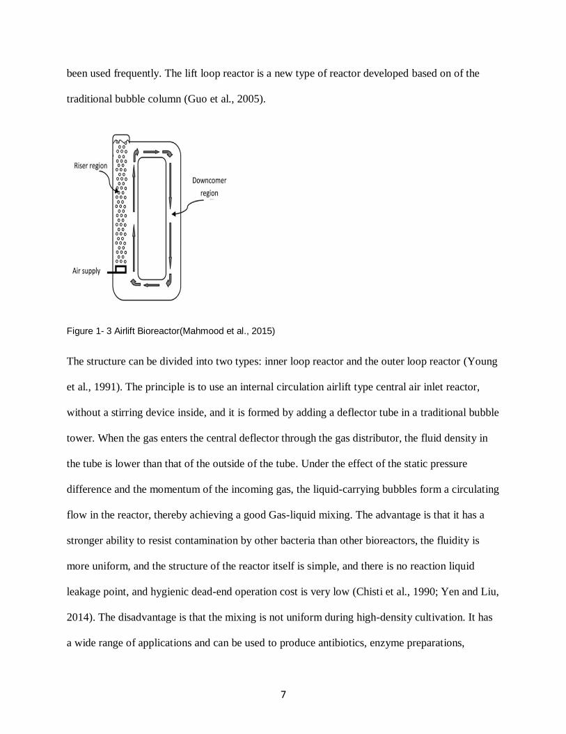
7
been used frequently. The lift loop reactor is a new type of reactor developed based on of the
traditional bubble column (Guo et al., 2005).
Figure 1- 3 Airlift Bioreactor(Mahmood et al., 2015)
The structure can be divided into two types: inner loop reactor and the outer loop reactor (Young
et al., 1991). The principle is to use an internal circulation airlift type central air inlet reactor,
without a stirring device inside, and it is formed by adding a deflector tube in a traditional bubble
tower. When the gas enters the central deflector through the gas distributor, the fluid density in
the tube is lower than that of the outside of the tube. Under the effect of the static pressure
difference and the momentum of the incoming gas, the liquid-carrying bubbles form a circulating
flow in the reactor, thereby achieving a good Gas-liquid mixing. The advantage is that it has a
stronger ability to resist contamination by other bacteria than other bioreactors, the fluidity is
more uniform, and the structure of the reactor itself is simple, and there is no reaction liquid
leakage point, and hygienic dead-end operation cost is very low (Chisti et al., 1990; Yen and Liu,
2014). The disadvantage is that the mixing is not uniform during high-density cultivation. It has
a wide range of applications and can be used to produce antibiotics, enzyme preparations,
8
organic acids, biological pesticides, edible fungi, single-cell protein production, etc (Yen and
Liu, 2014).
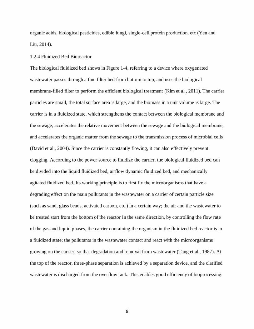
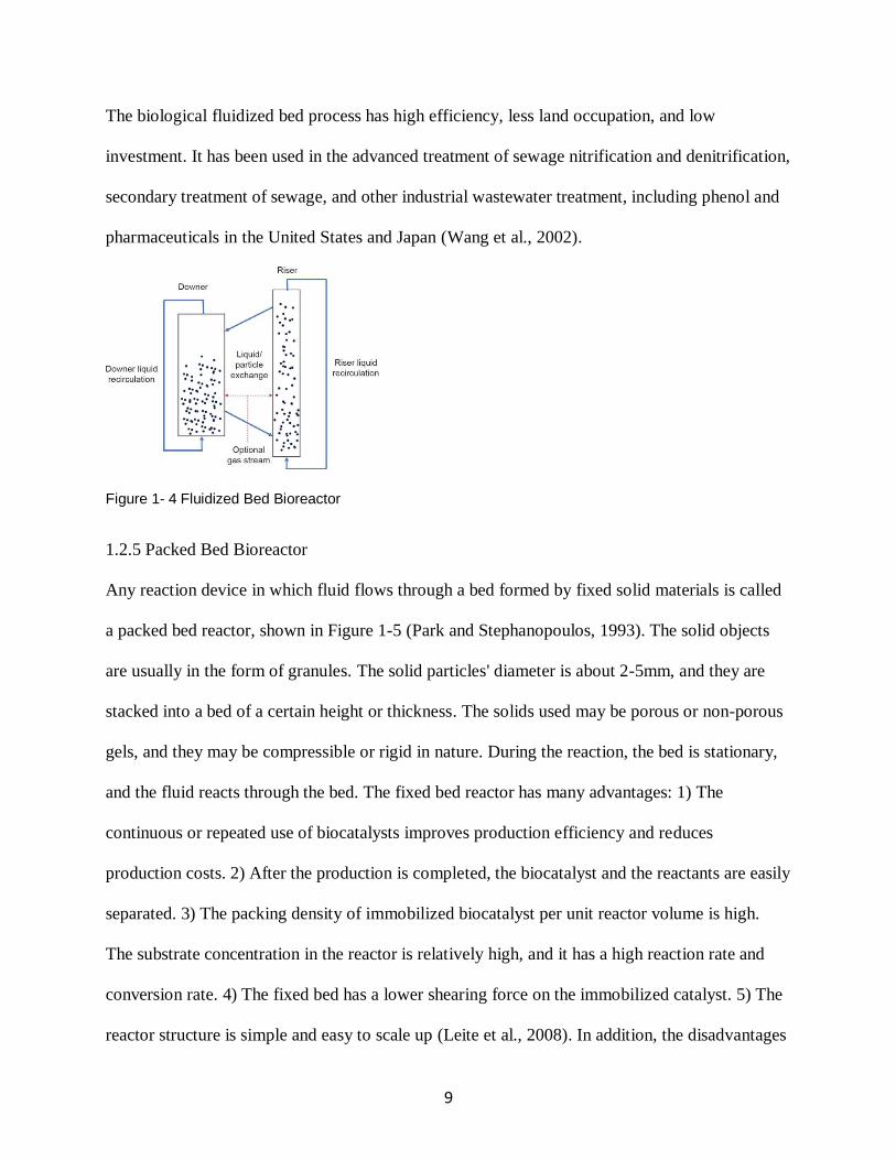
1.2.4 Fluidized Bed Bioreactor
The biological fluidized bed shows in Figure 1-4, referring to a device where oxygenated
wastewater passes through a fine filter bed from bottom to top, and uses the biological
membrane-filled filter to perform the efficient biological treatment (Kim et al., 2011). The carrier
particles are small, the total surface area is large, and the biomass in a unit volume is large. The
carrier is in a fluidized state, which strengthens the contact between the biological membrane and
the sewage, accelerates the relative movement between the sewage and the biological membrane,
and accelerates the organic matter from the sewage to the transmission process of microbial cells
(David et al., 2004). Since the carrier is constantly flowing, it can also effectively prevent
clogging. According to the power source to fluidize the carrier, the biological fluidized bed can
be divided into the liquid fluidized bed, airflow dynamic fluidized bed, and mechanically
agitated fluidized bed. Its working principle is to first fix the microorganisms that have a
degrading effect on the main pollutants in the wastewater on a carrier of certain particle size
(such as sand, glass beads, activated carbon, etc.) in a certain way; the air and the wastewater to
be treated start from the bottom of the reactor In the same direction, by controlling the flow rate
of the gas and liquid phases, the carrier containing the organism in the fluidized bed reactor is in
a fluidized state; the pollutants in the wastewater contact and react with the microorganisms
growing on the carrier, so that degradation and removal from wastewater (Tang et al., 1987). At
the top of the reactor, three-phase separation is achieved by a separation device, and the clarified
wastewater is discharged from the overflow tank. This enables good efficiency of bioprocessing.
9
The biological fluidized bed process has high efficiency, less land occupation, and low
investment. It has been used in the advanced treatment of sewage nitrification and denitrification,
secondary treatment of sewage, and other industrial wastewater treatment, including phenol and
pharmaceuticals in the United States and Japan (Wang et al., 2002).
Figure 1- 4 Fluidized Bed Bioreactor
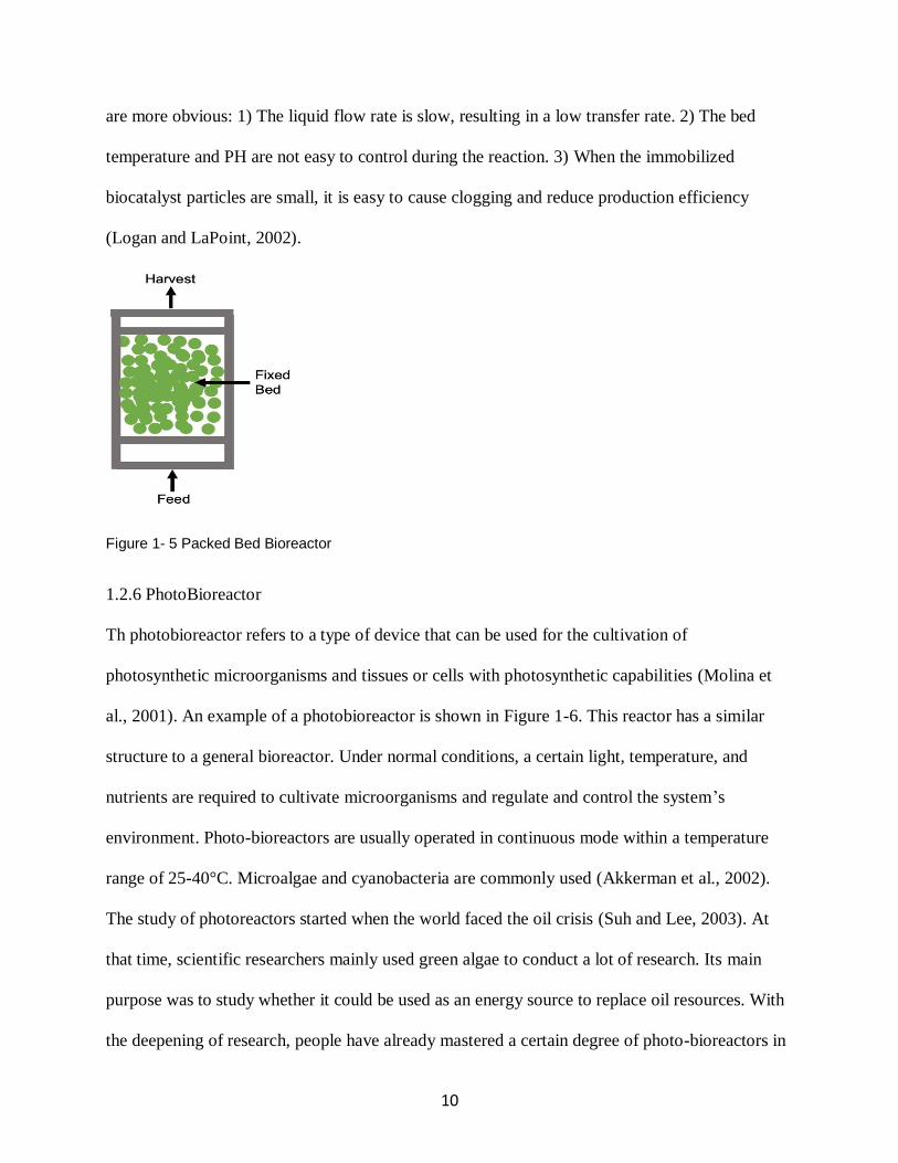
1.2.5 Packed Bed Bioreactor
Any reaction device in which fluid flows through a bed formed by fixed solid materials is called
a packed bed reactor, shown in Figure 1-5 (Park and Stephanopoulos, 1993). The solid objects
are usually in the form of granules. The solid particles' diameter is about 2-5mm, and they are
stacked into a bed of a certain height or thickness. The solids used may be porous or non-porous
gels, and they may be compressible or rigid in nature. During the reaction, the bed is stationary,
and the fluid reacts through the bed. The fixed bed reactor has many advantages: 1) The
continuous or repeated use of biocatalysts improves production efficiency and reduces
production costs. 2) After the production is completed, the biocatalyst and the reactants are easily
separated. 3) The packing density of immobilized biocatalyst per unit reactor volume is high.
The substrate concentration in the reactor is relatively high, and it has a high reaction rate and
conversion rate. 4) The fixed bed has a lower shearing force on the immobilized catalyst. 5) The
reactor structure is simple and easy to scale up (Leite et al., 2008). In addition, the disadvantages
10
are more obvious: 1) The liquid flow rate is slow, resulting in a low transfer rate. 2) The bed
temperature and PH are not easy to control during the reaction. 3) When the immobilized
biocatalyst particles are small, it is easy to cause clogging and reduce production efficiency
(Logan and LaPoint, 2002).
Figure 1- 5 Packed Bed Bioreactor
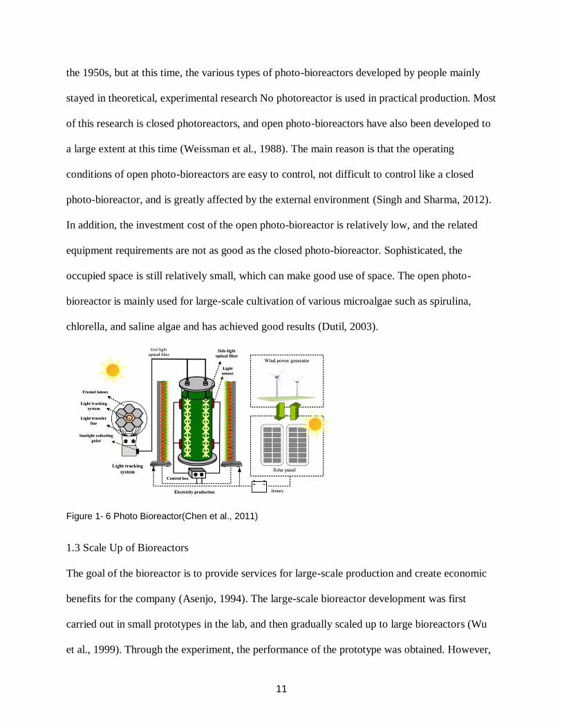
1.2.6 PhotoBioreactor
Th photobioreactor refers to a type of device that can be used for the cultivation of
photosynthetic microorganisms and tissues or cells with photosynthetic capabilities (Molina et
al., 2001). An example of a photobioreactor is shown in Figure 1-6. This reactor has a similar
structure to a general bioreactor. Under normal conditions, a certain light, temperature, and
nutrients are required to cultivate microorganisms and regulate and control the system’s
environment. Photo-bioreactors are usually operated in continuous mode within a temperature
range of 25-40°C. Microalgae and cyanobacteria are commonly used (Akkerman et al., 2002).
The study of photoreactors started when the world faced the oil crisis (Suh and Lee, 2003). At
that time, scientific researchers mainly used green algae to conduct a lot of research. Its main
purpose was to study whether it could be used as an energy source to replace oil resources. With
the deepening of research, people have already mastered a certain degree of photo-bioreactors in
11
the 1950s, but at this time, the various types of photo-bioreactors developed by people mainly
stayed in theoretical, experimental research No photoreactor is used in practical production. Most
of this research is closed photoreactors, and open photo-bioreactors have also been developed to
a large extent at this time (Weissman et al., 1988). The main reason is that the operating
conditions of open photo-bioreactors are easy to control, not difficult to control like a closed
photo-bioreactor, and is greatly affected by the external environment (Singh and Sharma, 2012).
In addition, the investment cost of the open photo-bioreactor is relatively low, and the related
equipment requirements are not as good as the closed photo-bioreactor. Sophisticated, the
occupied space is still relatively small, which can make good use of space. The open photo-
bioreactor is mainly used for large-scale cultivation of various microalgae such as spirulina,
chlorella, and saline algae and has achieved good results (Dutil, 2003).
Figure 1- 6 Photo Bioreactor(Chen et al., 2011)
1.3 Scale Up of Bioreactors
The goal of the bioreactor is to provide services for large-scale production and create economic
benefits for the company (Asenjo, 1994). The large-scale bioreactor development was first
carried out in small prototypes in the lab, and then gradually scaled up to large bioreactors (Wu
et al., 1999). Through the experiment, the performance of the prototype was obtained. However,
12
the data obtained from the prototype cannot often be obtained again in large-scale bioreactors.
This involves the problem of the reactor scale-up (Catapano et al., 2009). The bioreactor's scale-
up refers to the technology of transferring the optimized results in the research equipment to the
large-scale equipment. This is an important part of the biotechnology development process, and
also the industrialization of biotechnological achievements. The mixing time and mass transfer
coefficient (kLa) of the reactor show the performance of a bioreactor, so these two parameters are
particularly important in the scale-up of the bioreactor (Garcia-Ochoa and Gomez, 2009).
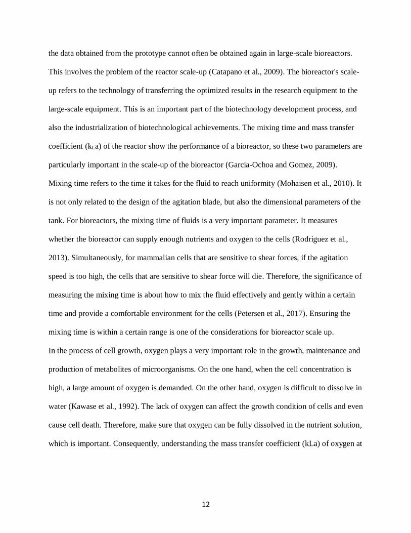
Mixing time refers to the time it takes for the fluid to reach uniformity (Mohaisen et al., 2010). It
is not only related to the design of the agitation blade, but also the dimensional parameters of the
tank. For bioreactors, the mixing time of fluids is a very important parameter. It measures
whether the bioreactor can supply enough nutrients and oxygen to the cells (Rodriguez et al.,
2013). Simultaneously, for mammalian cells that are sensitive to shear forces, if the agitation
speed is too high, the cells that are sensitive to shear force will die. Therefore, the significance of
measuring the mixing time is about how to mix the fluid effectively and gently within a certain
time and provide a comfortable environment for the cells (Petersen et al., 2017). Ensuring the
mixing time is within a certain range is one of the considerations for bioreactor scale up.
In the process of cell growth, oxygen plays a very important role in the growth, maintenance and
production of metabolites of microorganisms. On the one hand, when the cell concentration is
high, a large amount of oxygen is demanded. On the other hand, oxygen is difficult to dissolve in
water (Kawase et al., 1992). The lack of oxygen can affect the growth condition of cells and even
cause cell death. Therefore, make sure that oxygen can be fully dissolved in the nutrient solution,
which is important. Consequently, understanding the mass transfer coefficient (kLa) of oxygen at
13
different scales and different operating conditions plays an important role for the prediction the
growth of cell. And the prediction is critical to the scale-up of the reactor (Galaction et al., 2004).
In this study, through the experiment, mixing time and mass transfer coefficient (kLa) of 100L
prototype VDB, 100L prototype conventional reactor with continuous impeller and 100L
prototype conventional reactor with conventional impeller were characterized at different
volumes of simulated media, agitation speed and airflow rate, which provide a reference for the
scale-up and improvement of the reactors and impellers.
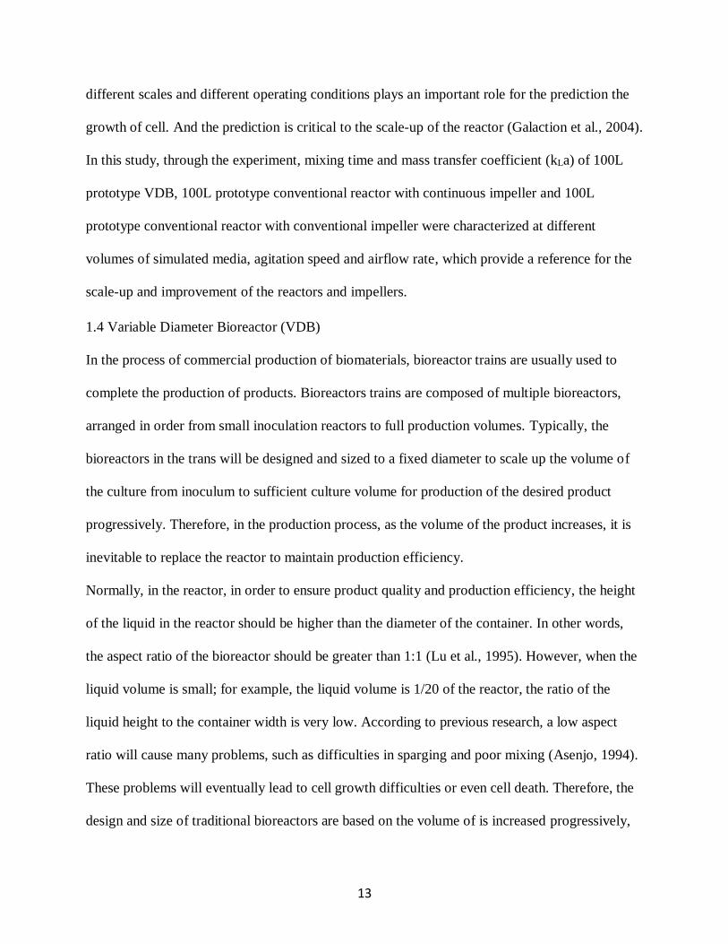
1.4 Variable Diameter Bioreactor (VDB)
In the process of commercial production of biomaterials, bioreactor trains are usually used to
complete the production of products. Bioreactors trains are composed of multiple bioreactors,
arranged in order from small inoculation reactors to full production volumes. Typically, the
bioreactors in the trans will be designed and sized to a fixed diameter to scale up the volume of
the culture from inoculum to sufficient culture volume for production of the desired product
progressively. Therefore, in the production process, as the volume of the product increases, it is
inevitable to replace the reactor to maintain production efficiency.
Normally, in the reactor, in order to ensure product quality and production efficiency, the height
of the liquid in the reactor should be higher than the diameter of the container. In other words,
the aspect ratio of the bioreactor should be greater than 1:1 (Lu et al., 1995). However, when the
liquid volume is small; for example, the liquid volume is 1/20 of the reactor, the ratio of the
liquid height to the container width is very low. According to previous research, a low aspect
ratio will cause many problems, such as difficulties in sparging and poor mixing (Asenjo, 1994).
These problems will eventually lead to cell growth difficulties or even cell death. Therefore, the
design and size of traditional bioreactors are based on the volume of is increased progressively,
14
until the volume of products in the bioreactor reaches the volume required for production. Since
the bioreactor is usually composed of stainless tanks, the volume is not variable, so multiple
bioreactors need to be used in the production process.
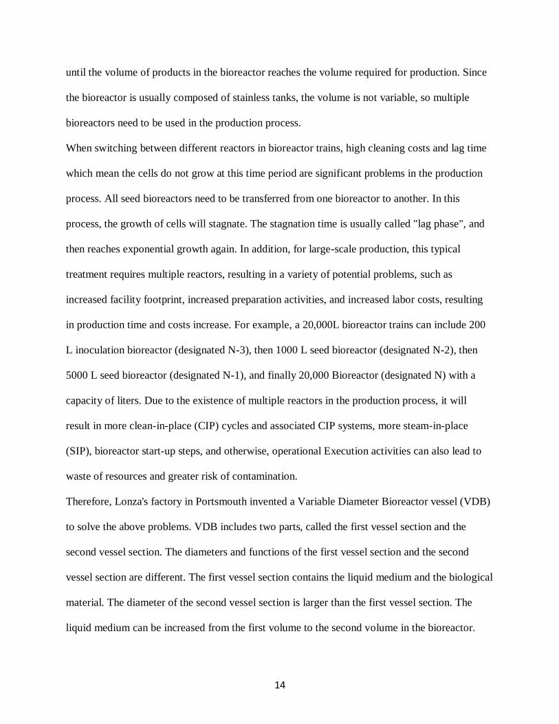
When switching between different reactors in bioreactor trains, high cleaning costs and lag time
which mean the cells do not grow at this time period are significant problems in the production
process. All seed bioreactors need to be transferred from one bioreactor to another. In this
process, the growth of cells will stagnate. The stagnation time is usually called "lag phase", and
then reaches exponential growth again. In addition, for large-scale production, this typical
treatment requires multiple reactors, resulting in a variety of potential problems, such as
increased facility footprint, increased preparation activities, and increased labor costs, resulting
in production time and costs increase. For example, a 20,000L bioreactor trains can include 200
L inoculation bioreactor (designated N-3), then 1000 L seed bioreactor (designated N-2), then
5000 L seed bioreactor (designated N-1), and finally 20,000 Bioreactor (designated N) with a
capacity of liters. Due to the existence of multiple reactors in the production process, it will
result in more clean-in-place (CIP) cycles and associated CIP systems, more steam-in-place
(SIP), bioreactor start-up steps, and otherwise, operational Execution activities can also lead to
waste of resources and greater risk of contamination.
Therefore, Lonza's factory in Portsmouth invented a Variable Diameter Bioreactor vessel (VDB)
to solve the above problems. VDB includes two parts, called the first vessel section and the
second vessel section. The diameters and functions of the first vessel section and the second
vessel section are different. The first vessel section contains the liquid medium and the biological
material. The diameter of the second vessel section is larger than the first vessel section. The
liquid medium can be increased from the first volume to the second volume in the bioreactor.
15
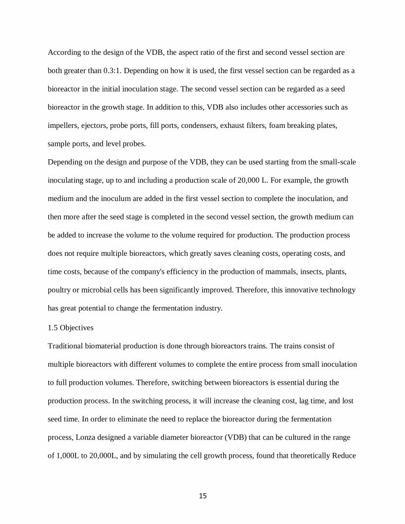
According to the design of the VDB, the aspect ratio of the first and second vessel section are
both greater than 0.3:1. Depending on how it is used, the first vessel section can be regarded as a
bioreactor in the initial inoculation stage. The second vessel section can be regarded as a seed
bioreactor in the growth stage. In addition to this, VDB also includes other accessories such as
impellers, ejectors, probe ports, fill ports, condensers, exhaust filters, foam breaking plates,
sample ports, and level probes.
Depending on the design and purpose of the VDB, they can be used starting from the small-scale
inoculating stage, up to and including a production scale of 20,000 L. For example, the growth
medium and the inoculum are added in the first vessel section to complete the inoculation, and
then more after the seed stage is completed in the second vessel section, the growth medium can
be added to increase the volume to the volume required for production. The production process
does not require multiple bioreactors, which greatly saves cleaning costs, operating costs, and
time costs, because of the company's efficiency in the production of mammals, insects, plants,
poultry or microbial cells has been significantly improved. Therefore, this innovative technology
has great potential to change the fermentation industry.
1.5 Objectives
Traditional biomaterial production is done through bioreactors trains. The trains consist of
multiple bioreactors with different volumes to complete the entire process from small inoculation
to full production volumes. Therefore, switching between bioreactors is essential during the
production process. In the switching process, it will increase the cleaning cost, lag time, and lost
seed time. In order to eliminate the need to replace the bioreactor during the fermentation
process, Lonza designed a variable diameter bioreactor (VDB) that can be cultured in the range
of 1,000L to 20,000L, and by simulating the cell growth process, found that theoretically Reduce
16
cell growth time by 2-5 days. This is very meaningful for industrial production. The long-term
goal of the project is to use this new bioreactor named VDB in the expansion facility of the
Lonza in Portsmouth after comprehensively evaluating its performance and improving the
design. Through CFD modeling, Lonza improved the design of VDB and continuous impeller,
then determined the final design. CFD modeling also shows that the fluid dynamic properties of
VDB are comparable to traditional bioreactors. But there is always a lack of experimental data to
verify it. In addition, parameters such as mass transfer coefficients (kLa) and mixing
characteristics, which are closely related to bioreactor properties, also need to be characterized.
Therefore, Lonza collaborated with the University of New Hampshire (UNH) to experimentally
characterize the properties of 100L VDB, 100L conventional reactor, and 100L conventional
reactor with novel continuous impeller, also compare the experimental results of three different
bioreactors, provide information for VDB's developing.
Chapter 2: Material and Method
2.1 Solution
Chemicals in this study is focusing on evaluating mixing time and mass transfer coefficient (kLa)
for VDB, conventional reactor with Continuous impeller and conventional reactor with
conventional impeller. 99% minimum Sodium Chloride (NaCl) purchased from Fisher, Pluronic
F68 contains oxyethylene, 79.9-83.7% purchased from Sigma, Sodium bicarbonate (NaHCO3)
contains 0.02% Calcium and 0.003% Chloride, 6M HCl and 1N NaOH purchased from Fisher.
2.1.1 Mixing Time
Vessel was filled with water, Sodium Chloride (NaCl) and Pluronic F68 were purchased from
Fisher (cat. S271-50) and SIGMA (cat. 15759) as surrogate media. pH standard from Radiometer
(cat. S11M002) was used to calibrate the pH sensors. HCl and NaOH from Fisher (cat. 60-047-

17
420, cat. 18-606-405) were used to adjust the pH value of the media. Air from Airgas is used to
adjust airflow according to testing parameters.
2.1.2 Mass Transfer Coefficient (kLa)
Vessel was filled with water, Sodium Chloride (NaCl), Pluronic F68 and Sodium bicarbonate
(NaHCO3) were purchased from Fisher (cat. S271-50) and SIGMA (cat. 15759) as surrogate
media. Air and pure N2 were purchased from Airgas to adjust dissolved oxygen (DO). Antifoam
media purchased from SIGMA (cat. A5757) was added when surrogate media overflowed from
vessel. In order not to affect the experimental results, add a minimum amount of antifoam media
according to the actual situation.
2.2 Fabrication of Bioreactor
2.2.1 Fabrication and Assembly
VDB, conventional bioreactor and impellers were designed and assembled by Lonza,
Portsmouth. Experiments were performed in University of New Hampshire.
2.1.1.1 VDB
Full capacity of VDB is 100L. Fig. 2.1 shows the Structure of VDB. The vessel is equipped with
a continuous tapered helix impeller and 4 baffles. VDB has 13 ports and valves in total, named
from P1 to P13. Where P4, P5, P6, P8, P10, P11 are sensor ports, P3, P7, P9 are sample ports.
Besides, P2 is sparger port to purge air or N2, P1 is agitator stabilizer port to hold impeller and
draining. P12 and P13 are additional ports, in this experiment, P13 was used to exhaust N2. It is
noted that the pH probes or DO probes are also installed to the sensor ports when conducting
mixing time measurements or mass transfer coefficient (kLa) measurements.
18
Figure 2- 1 Prototype of Assembled VDB
2.1.1.2 Conventional Reactor
Full capacity of VDB is 100L. Fig. 2-2 shows the main geometrical characteristics. Conventional
reactor has 4 baffles, and based on the needs, the vessel can be equipped with two different
impellers. One is a newly designed continuous impeller, the other is a conventional duel
impeller. Conventional reactor has 7 ports in total. P1 is draining port, P2 is sparge port to pump
air or N2, P3 is sample port, P4 and P5 are sensor ports. Two additional ports P6 and P7 are used
to exhaust air or N2 in this experiment. It is noted that the pH probes or DO probes are also
installed to the sensor ports when conducting mixing time measurements or mass transfer
coefficient (kLa) measurements.
19
Figure 2- 2 Prototype of Assembled Conventional Reactor
2.2.2 Assembly
In order to facilitate operation and drainage, VDB and conventional bioreactor are installed on a
designed cart and fixed around, which shows on Fig.2-3. The agitator motor is fixed directly
above the reactor, and the impeller is installed or removed by raising or lowering the agitator
motor. After bioreactor is installed, based on the volume of media, install the sensors on the
sensor ports and connect the sensor to control panel. It is noted that before the experiment starts,
all sensors installed need to be calibrated.
Figure 2- 3 Insolation of (a) Conventional Reactor and (b) VDB.
20
2.2.3 Data Collection
Real-time data will be collected by pH sensors and DO sensors, which were purchased from
MELLER TOLEDO (InPro 3250, InPro 6860I). During the experiment, all data will be uploaded
to the cloud server named Thingspeak through control panel. Both during and after the
experiment, the data can be downloaded. Data is analyzed by Microsoft Excel.
2.3 Method of mixing time calculation.
The mixing time(tM)is an important performance index of the bioreactors, and its definition is the
time required to achieve a certain degree of uniformity after the tracer material is injected into
the reactor. In this study, HCl is used as tracer material.
Mixing times is defined as the time when the concentration of OH- achieves within final
concentration with ±5% of its ultimate stable concentration (Eq. 2-1).
CRange=Cfinial ± 0.5x(Cinitial-Cfinal) Equation 2-1
Based on time, the first time point in this range is named tfinal. The time acid added is defined as
t0. Then mixing time can be obtained by using tfinal- t0 (Eq. 2-2).
tmixing= tfinal- t0 Equation 2-2
Based on the volume of surrogate media, HCl is added from P7 in VDB and P13 in conventional
reactor, adjust the media to pH 3 by using the required amount of HCl. When the pH stays steady
for three minutes or more, measurement ended. After each measurement, the required amount of
NaOH was added to restore the pH to its starting point. Each parameter is performed three
replicates, and the final result is averaged.
2.4 Method of kLa calculation.
Mass transfer coefficient (kLa), an important indicator of oxygen transfer efficiency in biological
reaction process (Linek et al., 1989). For many products, there is a close correspondence between
21
the oxygen transfer coefficient and the fermentation result (Puskeiler and Weuster-Botz, 2005).
Therefore, using KLa as the amplification criterion has become a widely accepted view in the
biochemical industry.
In literature, oxygen mass transfer is usually described by a simple transport law (Eq. 2-3)
(Gogate and Pandit, 1999; Özbek and Gayik, 2001).
dC/dt=OTR-OUR= kLa(C*-CL) Equation 2-3
dC/dt: the accumulation rate of oxygen in the liquid
OTR: the oxygen mass transfer rate from the gas bubble to the liquid
OUR: the oxygen uptake rate by the cells
kL: oxygen mass transfer coefficient
a: specific interfacial area
C*: saturated oxygen concentration
CL: dissolved oxygen concentration in the liquid
kLa is the product of the oxygen mass transfer coefficient KL and the gas-liquid specific surface
area “a”. Because it is difficult to measure the foam gas-liquid specific surface area “a” in
practical applications, kLa is treated as a factor to facilitate actual fermentation control (Damiani
et al., 2014).
In this study, kLa is measured by dynamic method. Experimental determination of kLa can be
achieved by recording the dissolved oxygen (DO) at different times after purging the bioreactor
with nitrogen (Wang and Zhong, 1996). Surrogate media is designed by Lonza and having
similar properties to the culture broth, chemicals are listed in Table 3. Because no cells are added
during the experiment, the oxygen consumption term OUR in Equation 1 is zero. After
22
integration of Equation 1, Equation 2 is for calculation KLa for a process with increasing DO
concentration from an initial value C0.
ln((C*-CL)/ C*-C0) = -kLat Equation 2-4
For each test, after vessel is filled with surrogate media, since kLa is related to temperature, the
temperature was controlled between 34.5°C and 38.5°C during the experiment. N2 will be purged
into vessel from P2 in VDB and conventional reactor until the control panel shows the DO is
lower than 5%. Then air will be sparged into the vessel from P2 until DO reaches 80% or higher.
Then measurement end. for each measurement, repeat the steps. Each parameter is performed
three replicates, and the final result is averaged.
Chapter 3: Results and Discussion
3.1 Mixing Time
3.1.1 Determination of the Mixing Time Point
We transfer the pH value received from the sensors into the ion concentration to find the mixing
time. pH value is transferred to the concentration of H+ and OH- by using the equation 10(-pH) and
10(-14+ pH). When the ion concentration reaches the range and stable, the time point the ion
concentration reached the range was recorded as the end of the test. The range was shown in
Eq.3-1.
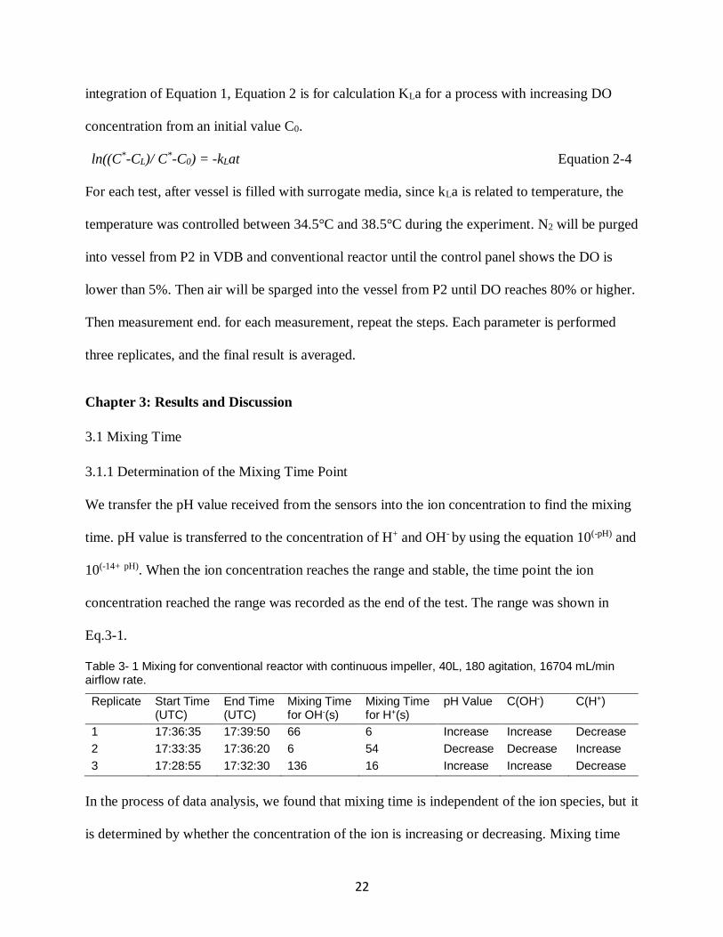
Table 3- 1 Mixing for conventional reactor with continuous impeller, 40L, 180 agitation, 16704 mL/min airflow rate.
Replicate Start Time (UTC)
End Time (UTC)
Mixing Time for OH-(s)
Mixing Time for H+(s)
pH Value
C(OH-)
C(H+)
1 17:36:35 17:39:50 66 6 Increase Increase Decrease
2 17:33:35 17:36:20 6 54 Decrease Decrease Increase
3 17:28:55 17:32:30 136 16 Increase Increase Decrease
In the process of data analysis, we found that mixing time is independent of the ion species, but it
is determined by whether the concentration of the ion is increasing or decreasing. Mixing time
23
derived from the ion with decreasing concentration is much shorter; while that from the ion with
increasing concentration is longer and often has overshooting peaks. For example, as we shown
in Table 3-1, conventional reactor with continuous impeller at 40L, 180 RPM, 16704mL/min
airflow rate was selected. In replicate 1, NaOH was used as pH tracer material. The
concentration of OH- increase and H- decrease. When the concentration of OH- and H+ reached
the range, the mixing time was determined as 66 seconds and 6 seconds. Mixing time derived
from the H+ with decreasing concentration is much shorter. In replicate 2, HCl was used as pH
tracer material, the concentration of OH- decrease and H- increase. When the concentration of
OH- and H+ reached the range, the mixing time was determined as 6 seconds and 54 seconds.
Mixing time derived from the OH- with decreasing concentration is much shorter. Same results
can be found in replicate 3, mixing time derived from the H+ with decreasing concentration is
much shorter, which is 16 seconds.
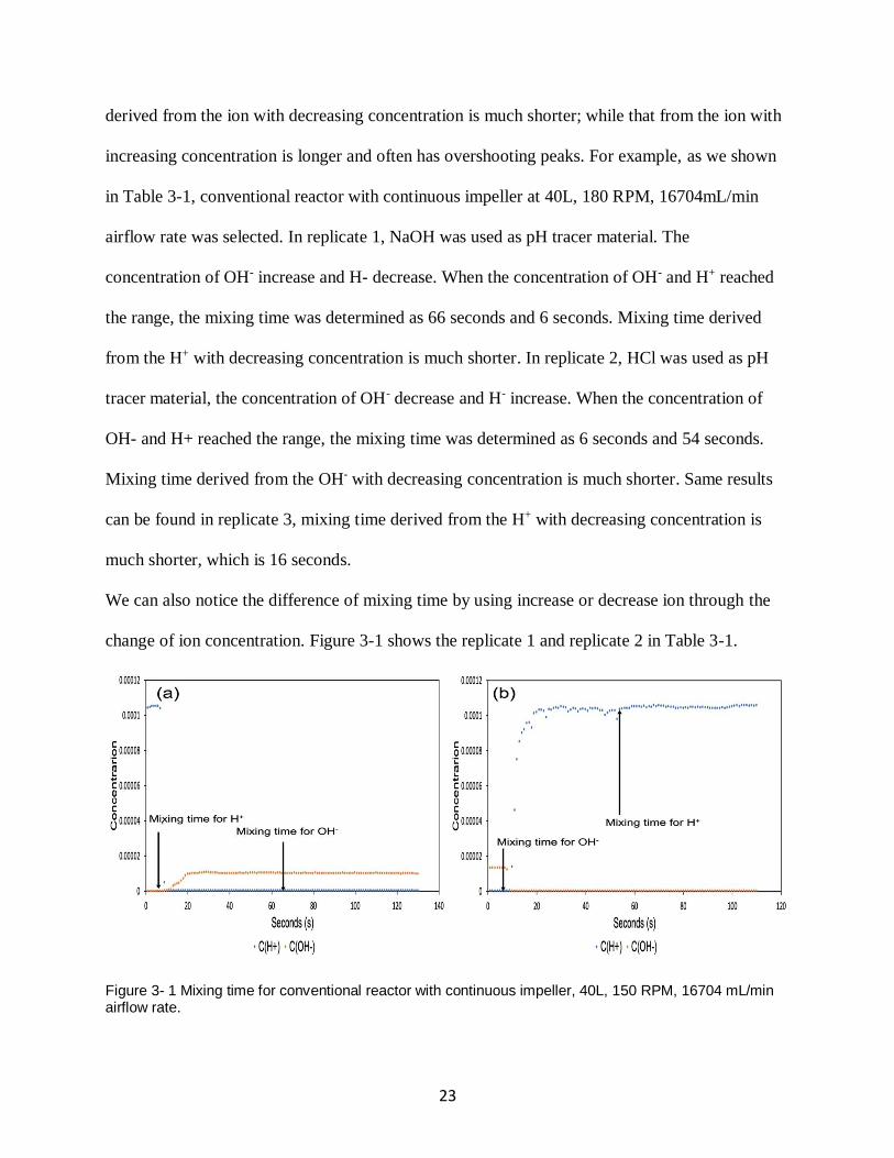
We can also notice the difference of mixing time by using increase or decrease ion through the
change of ion concentration. Figure 3-1 shows the replicate 1 and replicate 2 in Table 3-1.
Figure 3- 1 Mixing time for conventional reactor with continuous impeller, 40L, 150 RPM, 16704 mL/min airflow rate.
24
In replicate 1, the concentration of OH- increase and the concentration of H+ decrease. After we
plot the change of centration and marked the mixing time, we can notice that the mixing time for
H+ is shorter. In replicate 2, the concentration of H+ increase and the concentration of OH-
decrease. After we plot the change of centration and marked the mixing time, we can notice that
the mixing time for OH- is shorter. Therefore, mixing time is independent of the ion species, but
it is determined by whether the concentration of the ion is increasing or decreasing. This result
can be proved by the mathematic way.
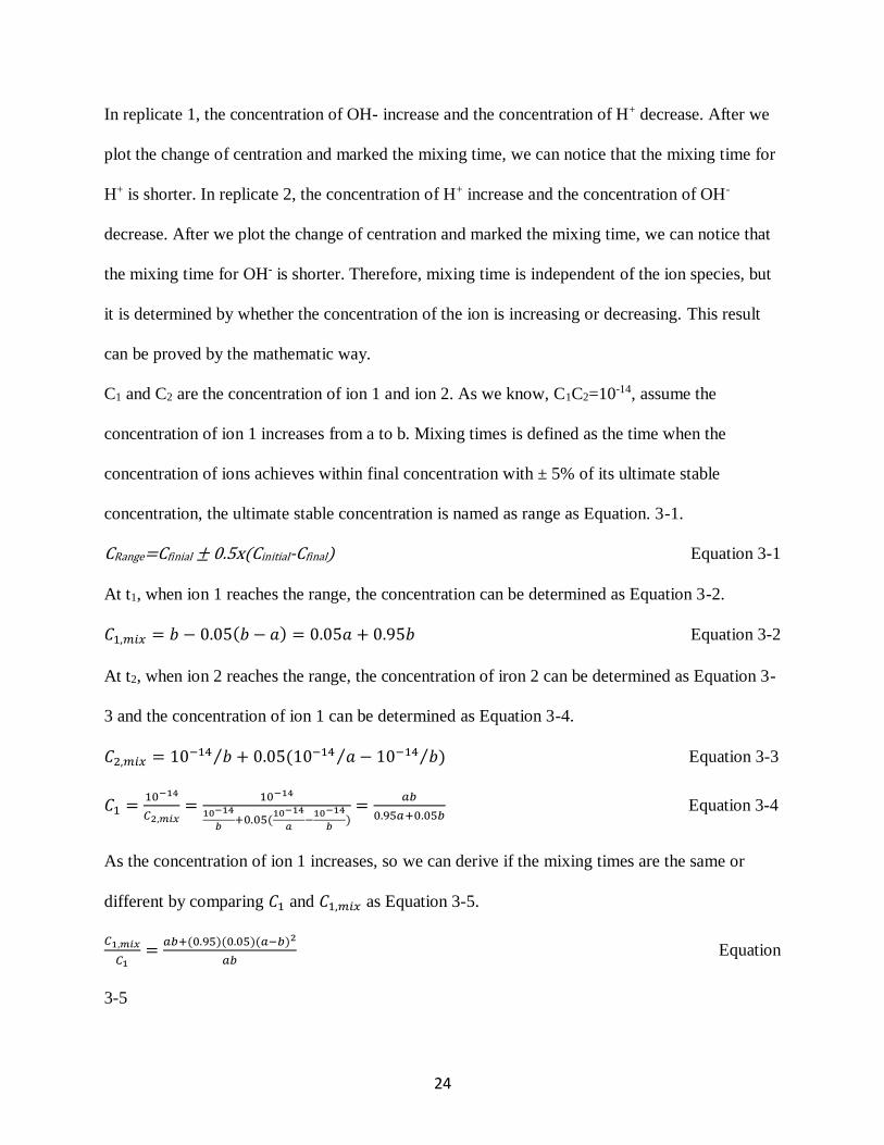
C1 and C2 are the concentration of ion 1 and ion 2. As we know, C1C2=10-14, assume the
concentration of ion 1 increases from a to b. Mixing times is defined as the time when the
concentration of ions achieves within final concentration with ± 5% of its ultimate stable
concentration, the ultimate stable concentration is named as range as Equation. 3-1.
CRange=Cfinial ± 0.5x(Cinitial-Cfinal) Equation 3-1
At t1, when ion 1 reaches the range, the concentration can be determined as Equation 3-2.
𝐶1,𝑚𝑖𝑥 = 𝑏 − 0.05(𝑏 − 𝑎) = 0.05𝑎 + 0.95𝑏 Equation 3-2
At t2, when ion 2 reaches the range, the concentration of iron 2 can be determined as Equation 3-
3 and the concentration of ion 1 can be determined as Equation 3-4.
𝐶2,𝑚𝑖𝑥 = 10−14 𝑏⁄ + 0.05(10−14 𝑎⁄ − 10−14 𝑏⁄ ) Equation 3-3
𝐶1 =10−14
𝐶2,𝑚𝑖𝑥=
10−14
10−14
𝑏+0.05(
10−14
𝑎−
10−14
𝑏)
=𝑎𝑏
0.95𝑎+0.05𝑏 Equation 3-4
As the concentration of ion 1 increases, so we can derive if the mixing times are the same or
different by comparing 𝐶1 and 𝐶1,𝑚𝑖𝑥 as Equation 3-5.
𝐶1,𝑚𝑖𝑥
𝐶1=
𝑎𝑏+(0.95)(0.05)(𝑎−𝑏)2
𝑎𝑏 Equation
3-5
25
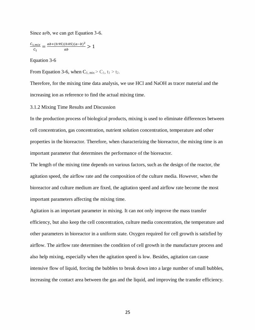
Since a≠b, we can get Equation 3-6.
𝐶1,𝑚𝑖𝑥
𝐶1=
𝑎𝑏+(0.95)(0.05)(𝑎−𝑏)2
𝑎𝑏> 1
Equation 3-6
From Equation 3-6, when C1, mix > C1, t1 > t2.
Therefore, for the mixing time data analysis, we use HCl and NaOH as tracer material and the
increasing ion as reference to find the actual mixing time.
3.1.2 Mixing Time Results and Discussion
In the production process of biological products, mixing is used to eliminate differences between
cell concentration, gas concentration, nutrient solution concentration, temperature and other
properties in the bioreactor. Therefore, when characterizing the bioreactor, the mixing time is an
important parameter that determines the performance of the bioreactor.
The length of the mixing time depends on various factors, such as the design of the reactor, the
agitation speed, the airflow rate and the composition of the culture media. However, when the
bioreactor and culture medium are fixed, the agitation speed and airflow rate become the most
important parameters affecting the mixing time.
Agitation is an important parameter in mixing. It can not only improve the mass transfer
efficiency, but also keep the cell concentration, culture media concentration, the temperature and
other parameters in bioreactor in a uniform state. Oxygen required for cell growth is satisfied by
airflow. The airflow rate determines the condition of cell growth in the manufacture process and
also help mixing, especially when the agitation speed is low. Besides, agitation can cause
intensive flow of liquid, forcing the bubbles to break down into a large number of small bubbles,
increasing the contact area between the gas and the liquid, and improving the transfer efficiency.
26
Therefore, the proper combination of impeller speed and aeration rate is significant important to
increase the manufacture efficiency of the product.
Since VDB and conventional reactor with continuous impeller are new designs, and there is no
experimental data reflecting their mixing efficiency. Therefore, the purpose of the mixing time
test is to compare the mixing efficiency between VDB, conventional reactor with continuous
impeller and conventional reactor with conventional impeller to find the best combination of
agitation speed and airflow rate. The agitation speed was selected based on the same power of
volume (P/V) in actual manufacture process, scale down the agitation speed to fit the test (Gill et
al., 2008). Combined with no airflow rate, low airflow rate and high airflow rate, collect
experimental data to achieve the purpose of the experiment. Different working conditions for
reactors, including volumes, airflow rates, and agitation speed are selected and shown in Table 3-
2.
Table 3- 2 Parameters for characterization of mixing time in 100L prototypes.
Bioreactor Type Agitation Speed (RPM)
Filling Volumes (L)
Airflow Setting (mL/min)
100L VDB 170, 200, 215, 305, 350
100L, 40L, 20L, 5L
0, 1113.6, 16704
100L conventional bioreactor with conventional impeller
30, 90, 120, 150, 180
100L, 40L 0, 1113.6, 16704
100L conventional bioreactor with continuous impeller
30, 90, 120, 150, 180
100L, 20L 0, 1113.6, 16704
3.1.2.1 Characterization of Mixing Time in 100L, 40L, 20L and 5L VDB
We first characterized the mixing time for VDB and evaluated the effect of agitation, airflow,
and volume on the mixing time. VDB filled with 100L, 40L, 20L, and 5L of the simulated
medium was used and the results were shown in Fig. 3-2. Generally, the mixing time decreases
as the agitation speed or the air flow rate goes up or the volume of VDB decreases, which is
anticipated since each of them is supposed to bring down the mixing time. However, when the
27
three factors work together, the extent one factor can reduce the mixing time is affected by the
other two.
Take the air flow rate as an example. The increase in the air flow rate significantly decrease the
mixing time when agitation is low (170 RPM) and the VDB is at the full volume of 100L. Under
this condition (Fig. 3-2(a)), the mixing time was 79 sec when there was no air. It drops sharply to
52 sec when the airflow rate was 1113.6 mL/min and further drops to 13 sec when the airflow
rate was16704 mL/min. The introduction of high airflow rate decreased the mixing time of full
volume VDB by 66 seconds when the agitation was 170 RPM. When the agitation speed
increased to 350 RPM for the VDB at the same full volume, the mixing time was 50 sec without
air, and it drops by 60% to 20 sec at high airflow rate. Similar effect can be seen from VDB run
at other volumes. At 40L (Fig. 3-2(b)) and low agitation (170 RPM), the mixing time is 67 sec
without air and it decreases by 50 sec to 17 sec, while at high agitation of 350 RPM under the
same volume, the mixing time was 25 sec without air, and slightly increases to 26 sec with
medium air flow and fluctuates to 24 sec with high airflow. The effect of air flow rate at high
28
agitation when the volume was 40L or lower was minimal.
Figure 3- 2 Mixing time for VDB at different agitation and airflow filled with (a) 100L, (b) 40L, (c) 20L, (d) 5L media.
Increasing agitation speed was anticipated to facilitate mixing. This was observed without air
flow (blue bars) or at medium airflow rate (orange bars), as shown in Fig. 3-2. Except for a
(a)
(b)
(c)
(d)
29
couple of outliers, the mixing time decreases as the agitation goes up from 170 RPM to 350
RPM, regardless of the volume. When there is no airflow, the mixing time drops from 79 sec to
48 sec with increasing rpm at full volume of 100L, 66 sec to 21 sec at 40L, 51 sec to 16 sec at
20L, and 21 sec to 9 sec at 5L. At medium airflow rate, the mixing time, as illustrated by the
orange bars, the mixing time drops from 51 sec to 19 sec at full volume of 100L, 42 sec to 21 sec
at 40L, 35 sec to 12 sec at 20L, and 12 sec to 5 sec at 5L. However, when the airflow rate was
high, as shown by the grey bars, the effect of agitation on the mixing time is not obvious. The
mixing time under high airflow rate with the same volume fluctuates within a small range. The
results show that the effect of airflow rate and agitation speed on the mixing time ties with each
other. The air flow rate can significantly reduce the mixing time under the low agitation speed,
but did not change it much under the high agitation speed. Similarly, the increase in agitation
speed results in a remarkable decrease in the mixing time with no or low airflow, while the
mixing time is not affected much by the agitation speed with high air flow rate. Both agitation
and air bubbling can facilitate the mixing until the mixing time reaches a lower limit.
30
Figure 3- 3 Mixing time for VDB at different volumes and airflow in (a) 170 RPM, (b) 200 RPM, (c) 215 RPM, (d) 305 RPM, (e) 350 RPM.
(d)
(c)
(a)
(b)
(e)
31
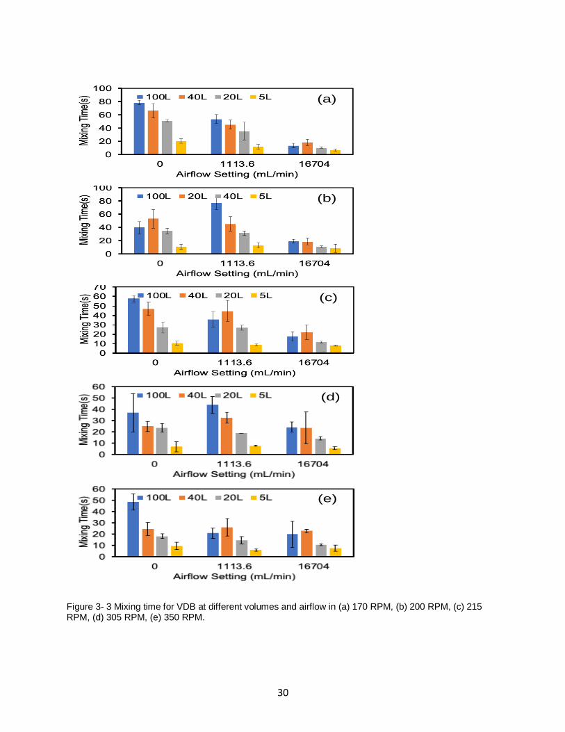
4 different volumes were tested. Fig. 3-3 showed the mixing time results for VDB at different
volumes and airflow in the agitation of 170 RPM, 200 RPM, 215 RPM, 305 RPM and 350 RPM.
As we described before, it can be seen from Fig.3-3 that when the airflow rate was low,
decreased the volume of simulated media in VDB can decrease the mixing time obviously. But
as the airflow rate increased from low to high, the effect of the volume on the mixing time
decreased.
Take the VDB at 170 RPM as the example in Fig 3-3 (a). When the agitation was set at 170
RPM, for the VDB filled with100L and 5L simulated media (blue bar and orange bar), mixing
time was 79 seconds and 18 seconds when there was no airflow. The mixing time reduced 61
seconds when the volume decreased from 100L to 5L. When the airflow rate increased to 16704
mL / min, when the volume decreased from 100L to 5L (blue bar and orange bar), the mixing
time always kept very close, which was about 10 seconds.
Similar results can be found at other agitation speed. For example, when the agitation speed was
305 RPM in Fig 3-3 (d), the mixing time for 100L and 5L VDB was 36 seconds and 8 seconds
when there was no airflow. The difference was 26 seconds. As the airflow rate increased to
1113.6 mL/min, the difference of mixing time was 31 seconds. Increased the airflow to 16704
mL/min, the difference of mixing time was 16 seconds. The results showed that when the
agitation speed was set, at high airflow rate, the influence of volume is slightly.
3.1.2.2 Characterization of Mixing Time in 100L and 20L Conventional Reactor with
Continuous Impeller
We characterized the mixing time for conventional reactor with continuous impeller and
evaluated the effect of agitation, airflow, and volume on the mixing time. Conventional reactor
filled with 100L, 20L of the simulated medium was used and the results were shown in Fig. 3-4.
32
Generally, the mixing time decreased as the airflow increase when the agitation speed was low.
And when the airflow rate was low, increased the agitation speed can reduce the mixing time
evidently. However, as the increase of agitation, the influence of airflow rate is decreased.
Besides, when the volume of conventional reactor is low, increased the agitation speed or airflow
rate cannot reduce the mixing time when there was airflow.
Take airflow rate as example. Fig. 3-4 (a) indicates that mixing time decreased when the airflow
increased, especially in 30 RPM, when the airflow increased from 0 to 16704 mL/min, mixing
time reduces 50 seconds. When the agitation speed increased to 90 RPM, the results showed that
increased the airflow rate from 0 to 16704 mL/min, the mixing time only reduced 21 seconds.
Continued to increase the agitation speed to 180 RPM, the difference of mixing time at no
airflow and high airflow was only 12 seconds. Similar results can be found when the
conventional reactor was filled with 40L simulated media in Fig 3-4 (b). When the agitation
speed was higher than 30 RPM, no matter the condition of airflow, the mixing time was always
about 9 seconds. Collectively, the influence of airflow rate decreased as the increasing of
agitation speed.
Increasing agitation speed can reduce mixing time when the reactor was filled with 100L or 20L
media. This was observed without airflow (blue bars) as shown in Fig. 3-4 (a) and Fig. 3-4 (b).
When there is no air flow, the mixing time drops from 92 sec to 21 sec with increasing agitation
speed at full volume of 100L and 34 sec to 10 sec at 20L. When the agitation speed was 30 RPM
and the volume was 20L, the mixing time dropped from 34 sec to 6 sec when increased airflow
rate from 0 to 1113.6 mL/min. Kept increasing airflow, the mixing time was still about 7 sec.
Both increased the airflow rate and agitation speed, the mixing time reduced slightly and was
always about 8 sec.
33
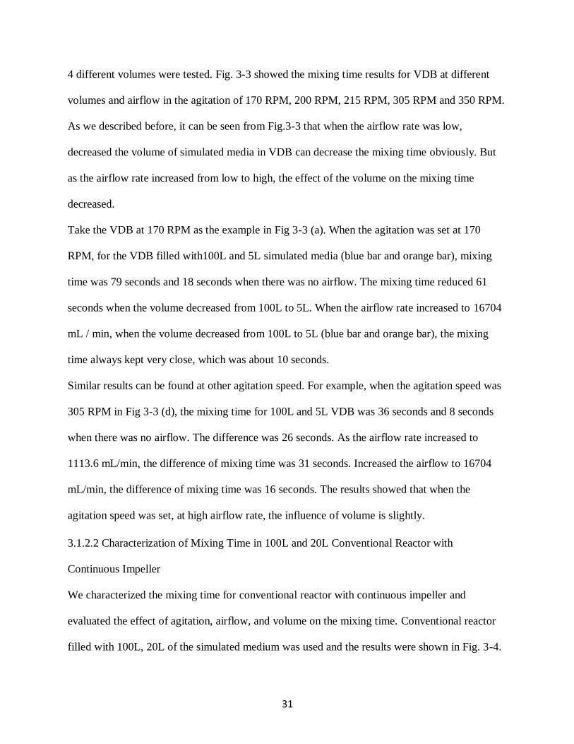
Figure 3- 4 Mixing time for conventional reactor with continuous impeller at different agitation and airflow filled with (a) 100L, (b) 20L media.
Fig.3-5 showed the mixing time results for conventional reactor with continuous impeller at
different volumes and airflow in the agitation of 30 RPM, 90 RPM, 120 RPM, 150 RPM and 180
RPM. The results suggested that increased the agitation speed or the airflow rate, the influence of
volume in mixing time can be reduced.
When there was no airflow (blue bar), the difference of mixing time between 100L and 20L was
61 sec in Fig 3-5 (a). Increased the agitation speed to 180 RPM, in Fig 3-5 (e), the difference of
mixing time between 100L and 20L was 14 sec.
34
Figure 3- 5 Mixing time for conventional reactor with continuous impeller at different volumes and airflow in (a) 30 RPM, (b) 90 RPM, (c) 120 RPM, (d) 150 RPM, (e) 180 RPM.
When the agitation speed was fixed, for example in Fig 3-5 (b), when there was no airflow, the
difference of mixing time between 100L and 20L was 21 sec. Increased the airflow to 1113.6
mL/min and 16704 mL/min, the difference of mixing time between 100L and 20L was 17 sec
and 6 sec. The similar results can be found at other agitation speed. Overall, in order to reduce
the influence of volume, increases the airflow rate and agitation speed have positive effect.
(d)
(c)
(b)
(a)
(e)
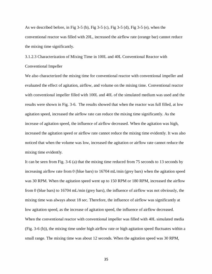
35
As we described before, in Fig 3-5 (b), Fig 3-5 (c), Fig 3-5 (d), Fig 3-5 (e), when the
conventional reactor was filled with 20L, increased the airflow rate (orange bar) cannot reduce
the mixing time significantly.
3.1.2.3 Characterization of Mixing Time in 100L and 40L Conventional Reactor with
Conventional Impeller
We also characterized the mixing time for conventional reactor with conventional impeller and
evaluated the effect of agitation, airflow, and volume on the mixing time. Conventional reactor
with conventional impeller filled with 100L and 40L of the simulated medium was used and the
results were shown in Fig. 3-6. The results showed that when the reactor was full filled, at low
agitation speed, increased the airflow rate can reduce the mixing time significantly. As the
increase of agitation speed, the influence of airflow decreased. When the agitation was high,
increased the agitation speed or airflow rate cannot reduce the mixing time evidently. It was also
noticed that when the volume was low, increased the agitation or airflow rate cannot reduce the
mixing time evidently.
It can be seen from Fig. 3-6 (a) that the mixing time reduced from 75 seconds to 13 seconds by
increasing airflow rate from 0 (blue bars) to 16704 mL/min (grey bars) when the agitation speed
was 30 RPM. When the agitation speed went up to 150 RPM or 180 RPM, increased the airflow
from 0 (blue bars) to 16704 mL/min (grey bars), the influence of airflow was not obviously, the
mixing time was always about 18 sec. Therefore, the influence of airflow was significantly at
low agitation speed, as the increase of agitation speed, the influence of airflow decreased.
When the conventional reactor with conventional impeller was filled with 40L simulated media
(Fig. 3-6 (b)), the mixing time under high airflow rate or high agitation speed fluctuates within a
small range. The mixing time was about 12 seconds. When the agitation speed was 30 RPM,
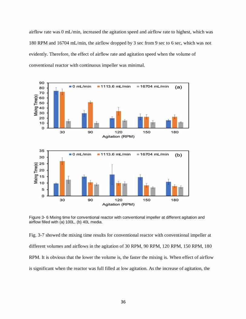
36
airflow rate was 0 mL/min, increased the agitation speed and airflow rate to highest, which was
180 RPM and 16704 mL/min, the airflow dropped by 3 sec from 9 sec to 6 sec, which was not
evidently. Therefore, the effect of airflow rate and agitation speed when the volume of
conventional reactor with continuous impeller was minimal.
Figure 3- 6 Mixing time for conventional reactor with conventional impeller at different agitation and airflow filled with (a) 100L, (b) 40L media.
Fig. 3-7 showed the mixing time results for conventional reactor with conventional impeller at
different volumes and airflows in the agitation of 30 RPM, 90 RPM, 120 RPM, 150 RPM, 180
RPM. It is obvious that the lower the volume is, the faster the mixing is. When effect of airflow
is significant when the reactor was full filled at low agitation. As the increase of agitation, the
37
effect of airflow rate was low. And it was noticed that when the volume was low, the effect of
agitation speed or airflow rate on mixing time was not obviously.
Figure 3- 7 Mixing time for conventional reactor with conventional impeller at different volumes and airflow in (a) 30 RPM, (b) 90 RPM, (c) 120 RPM, (d) 150 RPM, (e) 180 RPM.
Take the airflow rate as an example. In Fig 3-7 (a), when the reactor was full filled, increased the
airflow from 0 mL/ min to 16704 mL/ min, the mixing time reduced by 66 sec from 76 sec to 9
(c)
(b)
(a)
(d)
(e)
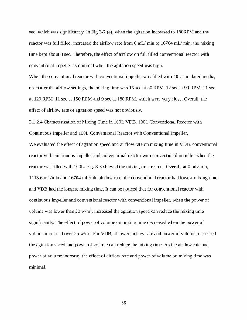
38
sec, which was significantly. In Fig 3-7 (e), when the agitation increased to 180RPM and the
reactor was full filled, increased the airflow rate from 0 mL/ min to 16704 mL/ min, the mixing
time kept about 8 sec. Therefore, the effect of airflow on full filled conventional reactor with
conventional impeller as minimal when the agitation speed was high.
When the conventional reactor with conventional impeller was filled with 40L simulated media,
no matter the airflow settings, the mixing time was 15 sec at 30 RPM, 12 sec at 90 RPM, 11 sec
at 120 RPM, 11 sec at 150 RPM and 9 sec at 180 RPM, which were very close. Overall, the
effect of airflow rate or agitation speed was not obviously.
3.1.2.4 Characterization of Mixing Time in 100L VDB, 100L Conventional Reactor with
Continuous Impeller and 100L Conventional Reactor with Conventional Impeller.
We evaluated the effect of agitation speed and airflow rate on mixing time in VDB, conventional
reactor with continuous impeller and conventional reactor with conventional impeller when the
reactor was filled with 100L. Fig. 3-8 showed the mixing time results. Overall, at 0 mL/min,
1113.6 mL/min and 16704 mL/min airflow rate, the conventional reactor had lowest mixing time
and VDB had the longest mixing time. It can be noticed that for conventional reactor with
continuous impeller and conventional reactor with conventional impeller, when the power of
volume was lower than 20 w/m3, increased the agitation speed can reduce the mixing time
significantly. The effect of power of volume on mixing time decreased when the power of
volume increased over 25 w/m3. For VDB, at lower airflow rate and power of volume, increased
the agitation speed and power of volume can reduce the mixing time. As the airflow rate and
power of volume increase, the effect of airflow rate and power of volume on mixing time was
minimal.
39
Fig. 3-8 (a) showed that for conventional reactor with continuous impeller and conventional
reactor with conventional impeller, when the power of volume increased from 0 w/m3 to 20
w/m3, mixing time for reduced by 40 seconds to 50 seconds, which was about 30. Continued to
increase the power of volume, the change of mixing time was minimal and always kept about 22
seconds. When the airflow rate was 0 mL/min, increased the power of volume from 10 w/m3 to
20 w/m3, the mixing time in VDB decreased from 80 seconds to 40 seconds. Continued to
increase the power of volume, the mixing time was always kept about 48 seconds. It was clearly
to see that when the airflow rate was 0, conventional reactor with continuous impeller always
had the lowest mixing time.
For all bioreactors at 1113.6 mL/min airflow rate (Fig. 3-8 (b)), the trend of mixing time results
was similar to the mixing time at 0 airflow. But there was an outlier for VDB when the power of
volume was 19 w/m3, and the mixing time went up to 80 seconds. It should be noticed that when
the airflow rate increased to 1113.6 mL/min, the conventional reactor with continuous impeller
had the lowest mixing time.
Fig. 3-8 (c) showed at 16704 mL/min airflow rate, 10 w/m3, mixing time in conventional reactor
with continuous impeller was high which was 37 seconds. When the power of volume increased
to 20 w/m3 and higher, the change of mixing time for conventional reactor with continuous
impeller and conventional reactor with conventional impeller was minimal and was always
maintained at 8 seconds. And conventional reactor with continuous impeller had the lowest
mixing time. Compared with the other two reactors, the mixing time of VDB cannot be affected
by power of volume, which was 20 seconds.
40
Figure 3- 8 Mixing time for VDB, conventional reactor with continuous impeller and conventional reactor with conventional impeller in 100L, (a) 0 airflow, (b) 1113.6 mL/min airflow and (c) 16704 mL/min airflow.
Overall, the mixing time of VDB was longer than conventional reactor with conventional
impeller and conventional reactor with continuous impeller. When the airflow rate was 0 and
1113.6 mL/min, the mixing time for conventional reactor with conventional impeller
conventional reactor with continuous impeller was close. Increased the airflow rate to 16704
mL/min, when the power of volume was higher than 10 w/m3, the mixing time for 3 bioreactors
was close.
41
3.1.2.5 Characterization of Mixing Time in 40L VDB and 40L Conventional Reactor with
Conventional Impeller.
Fig. 3-9 showed that mixing time for VDB was longer than conventional reactor with
conventional impeller at all power of volume setting and airflow settings in 40L. The results
suggested for VDB, when the airflow rate was low, as the increase of power of volume, the
mixing time decreased. For conventional reactor with conventional impeller, the effect of power
of volume and airflow rate on the mixing time was minimum. Overall, when the reactors were
filled with 40L, conventional reactor with conventional impeller had lower mixing time.
Fig. 3-9 (a) showed that as the increase of the power of volume, the mixing time for VDB
reduced significantly, the mixing time for conventional reactor with conventional impeller
maintained about 15 seconds, which makes the mixing time became close. But VDB always had
a longer mixing time. For example, at 20 w/m3, the difference of mixing time between two
reactors was about 60 seconds. But the mixing time gradually approached along with the
increase of power of volume. The difference of mixing time between VDB and conventional
reactor with conventional impeller was 10 seconds when the power of volume went up to 140
w/m3. And mixing time for VDB was 25 seconds, still 15 seconds higher than the mixing time in
conventional reactor with conventional impeller.
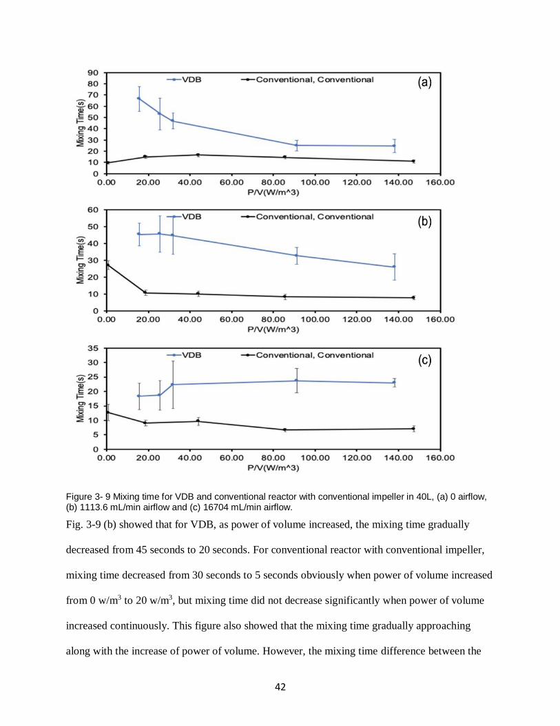
42
Figure 3- 9 Mixing time for VDB and conventional reactor with conventional impeller in 40L, (a) 0 airflow, (b) 1113.6 mL/min airflow and (c) 16704 mL/min airflow.
Fig. 3-9 (b) showed that for VDB, as power of volume increased, the mixing time gradually
decreased from 45 seconds to 20 seconds. For conventional reactor with conventional impeller,
mixing time decreased from 30 seconds to 5 seconds obviously when power of volume increased
from 0 w/m3 to 20 w/m3, but mixing time did not decrease significantly when power of volume
increased continuously. This figure also showed that the mixing time gradually approaching
along with the increase of power of volume. However, the mixing time difference between the
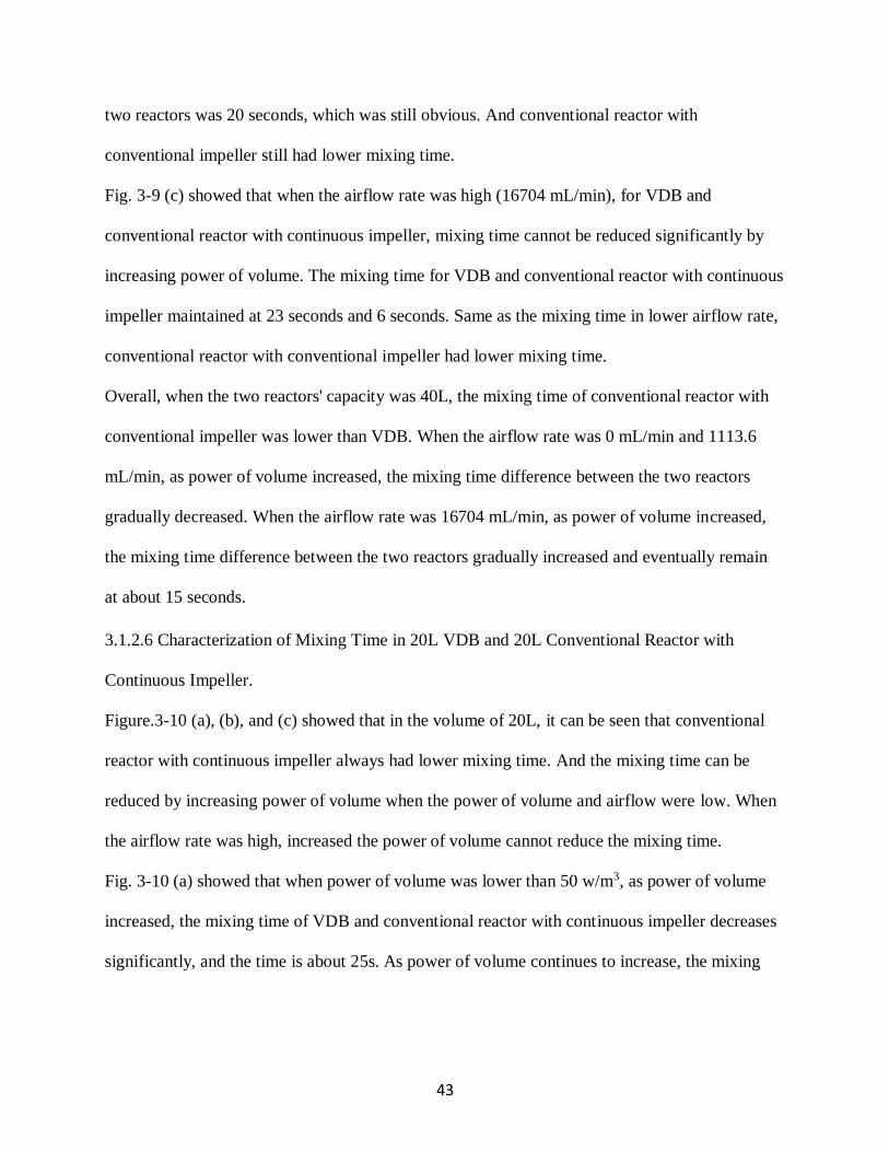
43
two reactors was 20 seconds, which was still obvious. And conventional reactor with
conventional impeller still had lower mixing time.
Fig. 3-9 (c) showed that when the airflow rate was high (16704 mL/min), for VDB and
conventional reactor with continuous impeller, mixing time cannot be reduced significantly by
increasing power of volume. The mixing time for VDB and conventional reactor with continuous
impeller maintained at 23 seconds and 6 seconds. Same as the mixing time in lower airflow rate,
conventional reactor with conventional impeller had lower mixing time.
Overall, when the two reactors' capacity was 40L, the mixing time of conventional reactor with
conventional impeller was lower than VDB. When the airflow rate was 0 mL/min and 1113.6
mL/min, as power of volume increased, the mixing time difference between the two reactors
gradually decreased. When the airflow rate was 16704 mL/min, as power of volume increased,
the mixing time difference between the two reactors gradually increased and eventually remain
at about 15 seconds.
3.1.2.6 Characterization of Mixing Time in 20L VDB and 20L Conventional Reactor with
Continuous Impeller.
Figure.3-10 (a), (b), and (c) showed that in the volume of 20L, it can be seen that conventional
reactor with continuous impeller always had lower mixing time. And the mixing time can be
reduced by increasing power of volume when the power of volume and airflow were low. When
the airflow rate was high, increased the power of volume cannot reduce the mixing time.
Fig. 3-10 (a) showed that when power of volume was lower than 50 w/m3, as power of volume
increased, the mixing time of VDB and conventional reactor with continuous impeller decreases
significantly, and the time is about 25s. As power of volume continues to increase, the mixing
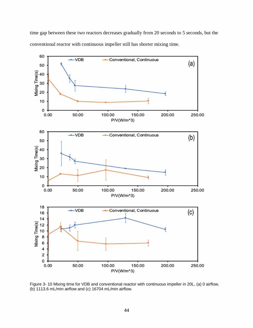
44
time gap between these two reactors decreases gradually from 20 seconds to 5 seconds, but the
conventional reactor with continuous impeller still has shorter mixing time.
Figure 3- 10 Mixing time for VDB and conventional reactor with continuous impeller in 20L, (a) 0 airflow, (b) 1113.6 mL/min airflow and (c) 16704 mL/min airflow.
45
Fig. 3-10 (b) showed that when the power of volume was lower than 50 w/m3, the mixing time
for the two bioreactors had a significant difference, which was 25 seconds. As power of volume
increased over 150 w/m3, the mixing time difference gradually decreased. The difference was
only 3 seconds. And it should be noticed that the effect of power of volume on mixing time was
minimum. For example, increased the power of volume from 0 to 170, for conventional reactor
with continuous impeller, the mixing time was about 5 seconds. Conventional reactor with
continuous impeller had lower mixing time.
It was shown in figure.3-10 (c) that the mixing time for VDB and conventional reactor with
continuous impeller was close when the power of volume was lower than 50 w/m3, the mixing
time was about 10 seconds. As the increased power of volume, the mixing time of the
conventional reactor with continuous impeller dropped 6 seconds from 12 seconds to 6 seconds.
The mixing time of VDB maintained at 12 seconds. The mixing time in two reactors cannot be
reduced by increasing the power of volume, and conventional reactor with continuous impeller
had lower mixing time.
Overall, when the capacity of the two reactors was 20L, the mixing time performance of
conventional reactor with continuous impeller was better than VDB. When the airflow rate was
high, the mixing time for VDB and conventional reactor with continuous impeller cannot be
reduced significantly by increasing power of volume.
3.2 Mass Transfer Coefficient (kLa)
During the production of biological products, the oxygen in the air must be dissolved in the liquid
first and then used by the microorganisms. There is a close correspondence between the oxygen
transfer coefficient (kLa) and the fermentation result for many products. One of the bioreactor
functions is to provide sufficient dissolved oxygen to meet the needs of microorganisms. Therefore,

46
the oxygen transfer efficiency is usually considered to be the main problem in the selection and
design of bioreactors. As an important character of oxygen transfer efficiency in biological
reaction process, kLa has been widely accepted by biochemical industry to analyze oxygen transfer
efficiency.
Many factors affect kLa, such as the structure of the reactor, the agitation speed and the airflow
rate. Therefore, this experiment uses different agitation speeds and airflow rates to characterize
kLa of new designed VDB, conventional reactor with continuous impeller and conventional
reactor with conventional impeller in different volumes, agitation speed and airflow rate. By
comparing the kLa between the three reactors, provides a reference for the design of the reactor
in the future. The agitation speed was selected based on the same power of volume (P/V) in
actual manufacture process, scale down the agitation speed to fit the test. Combined with
different airflow rates, collect experimental data to achieve the purpose of the experiment. The
measured parameters are listed in the Table 3-3.
Table 3- 3 Parameters for characterization of mass transfer coefficient (kLa) in 100L prototypes.
Bioreactor Type Agitation Speed (RPM)
Filling Volumes (L)
Airflow Setting (mL/min)
100L VDB 170, 200, 215,
305, 350
100L, 40L, 20L,
5L
1113.6, 5568, 11136,
16704 100L conventional bioreactor
with conventional impeller
30, 90, 120, 150,
180
100L, 40L 1113.6, 5568, 11136,
16704
100L conventional bioreactor
with continuous impeller
30, 90, 120, 150,
180
100L, 20L 1113.6, 5568, 11136,
16704
3.2.1 Characterization of Mass Transfer Coefficient (kLa) in 100L, 40L, 20L and 5L VDB
We first characterized the kLa for VDB and evaluated the effect of agitation and airflow on the
kLa. VDB filled with 100L, 40L, 20L, and 5L of the simulated medium was used and the results
were shown in Fig. 3-11. Generally, the kLa increased as the agitation speed or the airflow rate
went up, which is anticipated since each of them is supposed to have a positive effect on kLa.
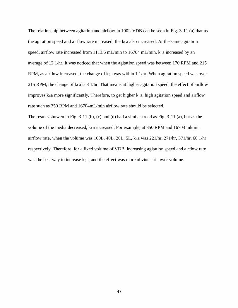
47
The relationship between agitation and airflow in 100L VDB can be seen in Fig. 3-11 (a) that as
the agitation speed and airflow rate increased, the kLa also increased. At the same agitation
speed, airflow rate increased from 1113.6 mL/min to 16704 mL/min, kLa increased by an
average of 12 1/hr. It was noticed that when the agitation speed was between 170 RPM and 215
RPM, as airflow increased, the change of kLa was within 1 1/hr. When agitation speed was over
215 RPM, the change of kLa is 8 1/hr. That means at higher agitation speed, the effect of airflow
improves kLa more significantly. Therefore, to get higher kLa, high agitation speed and airflow
rate such as 350 RPM and 16704mL/min airflow rate should be selected.
The results showen in Fig. 3-11 (b), (c) and (d) had a similar trend as Fig. 3-11 (a), but as the
volume of the media decreased, kLa increased. For example, at 350 RPM and 16704 ml/min
airflow rate, when the volume was 100L, 40L, 20L, 5L, kLa was 221/hr, 271/hr, 371/hr, 60 1/hr
respectively. Therefore, for a fixed volume of VDB, increasing agitation speed and airflow rate
was the best way to increase kLa, and the effect was more obvious at lower volume.
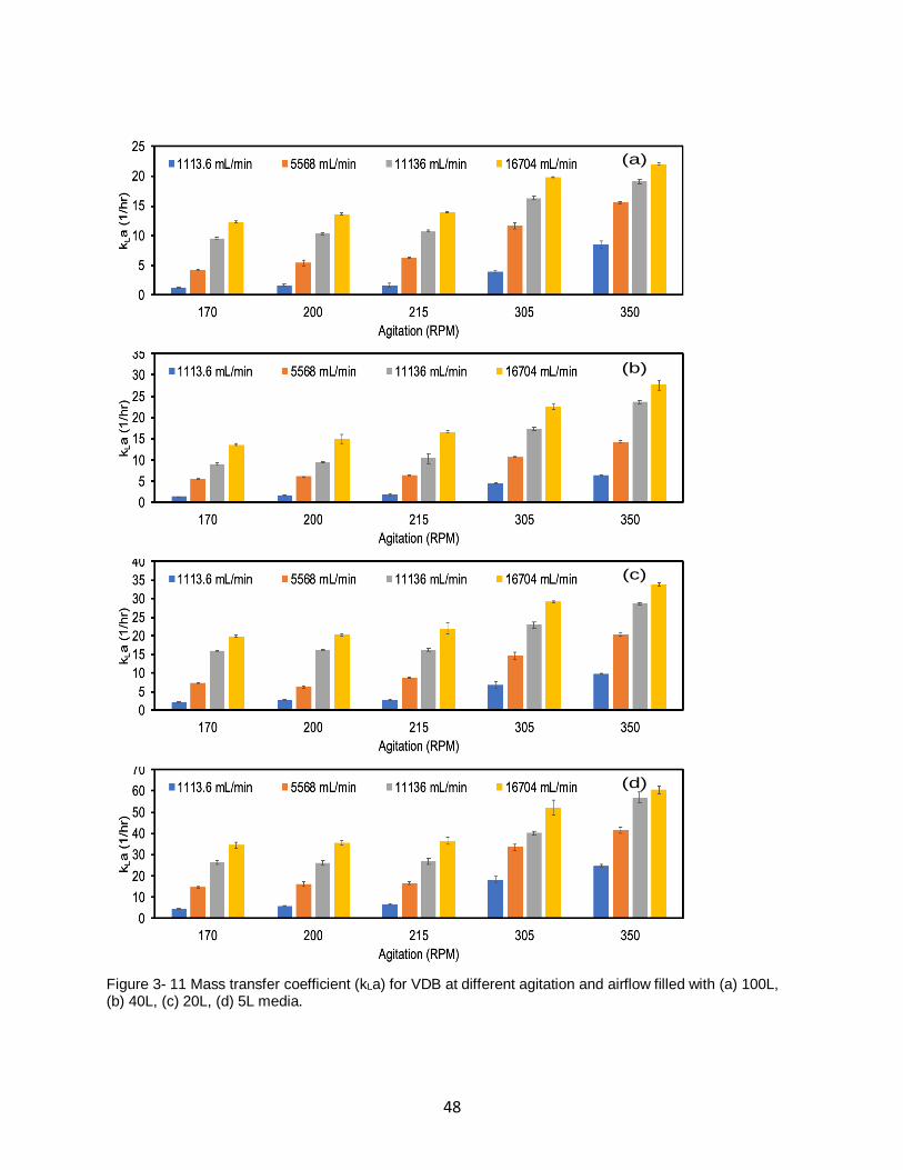
48
Figure 3- 11 Mass transfer coefficient (kLa) for VDB at different agitation and airflow filled with (a) 100L, (b) 40L, (c) 20L, (d) 5L media.
(d)
(c)
(a)
(b)
(a)
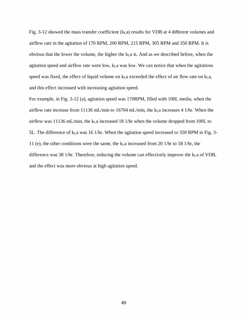
49
Fig. 3-12 showed the mass transfer coefficient (kLa) results for VDB at 4 different volumes and
airflow rate in the agitation of 170 RPM, 200 RPM, 215 RPM, 305 RPM and 350 RPM. It is
obvious that the lower the volume, the higher the kLa is. And as we described before, when the
agitation speed and airflow rate were low, kLa was low. We can notice that when the agitations
speed was fixed, the effect of liquid volume on kLa exceeded the effect of air flow rate on kLa,
and this effect increased with increasing agitation speed.
For example, in Fig. 3-12 (a), agitation speed was 170RPM, filled with 100L media, when the
airflow rate increase from 11136 mL/min to 16704 mL/min, the kLa increases 4 1/hr. When the
airflow was 11136 mL/min, the kLa increased 18 1/hr when the volume dropped from 100L to
5L. The difference of kLa was 16 1/hr. When the agitation speed increased to 350 RPM in Fig. 3-
11 (e), the other conditions were the same, the kLa increased from 20 1/hr to 58 1/hr, the
difference was 38 1/hr. Therefore, reducing the volume can effectively improve the kLa of VDB,
and the effect was more obvious at high agitation speed.
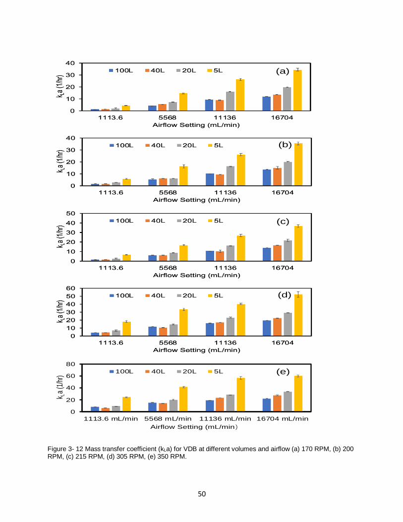
50
Figure 3- 12 Mass transfer coefficient (kLa) for VDB at different volumes and airflow (a) 170 RPM, (b) 200 RPM, (c) 215 RPM, (d) 305 RPM, (e) 350 RPM.
0
20
40
60
80
1113.6 mL/min 5568 mL/min 11136 mL/min 16704 mL/min
k La (1
/hr)
Airflow Setting (mL/min
100L 40L 20L 5L (e)
(d)
(c)
(b)
(a)

51
3.2.2 Characterization of Mass Transfer Coefficient (kLa) in 100L and 20L Conventional Reactor
with Continuous Impeller
Fig. 3-13 showed the mass transfer coefficient (kLa) results for conventional reactor with
continuous impeller at different agitation and airflow settings in the volumes of 100L and 20L.
Overall, the relationship between airflow rate and agitation speed was more linear in 100L
conventional reactor with continuous impeller. As the increases of airflow and agitation speed,
the kLa increases.
When the conventional reactor filled with 100L simulated media, the effect of airflow on kLa
was more obvious when the agitation speed was high. Similarly, when the air flow was high, the
effect of the agitation speed on kLa was also obvious. For example, in Fig. 3-13 (a), when the
agitation speed was 30 RPM, increased the airflow rate from 1113.6 mL/min to 16704 mL/min,
the kLa increased by 3 1/hr, from 1 1/hr to 4 1/hr. When the agitation speed went up to 180 RPM,
the kLa increased by 19 1/hr, from 10 1/hr to 29 1/hr.
Fig. 3-13 (b) showed increasing the agitation speed and airflow rate cannot always increase kLa
when the volume was 20L. The results suggested that when the agitation speed was between 30
RPM and 90 RPM, increased the airflow rate can improve the kLa efficiently. However, when
the agitation was 150RPM, the kLa increased from 5 1/hr to 18 1/hr when the airflow increased
from 1113.6 mL/min to 5568 mL/min. Continued increasing airflow, the kLa decreased first and
then increased, and the change was not obvious. When the agitation speed was 180 RPM, the
kLa remained 10 1/hr when airflow increased from 1113.6 mL/min to 5568 mL/min. It continued
increasing airflow rate up to 16704 mL/min, the kLa increased to 18 1/hr.
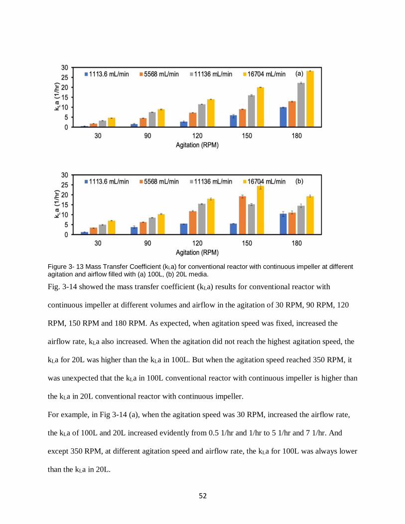
52
Figure 3- 13 Mass Transfer Coefficient (kLa) for conventional reactor with continuous impeller at different agitation and airflow filled with (a) 100L, (b) 20L media.
Fig. 3-14 showed the mass transfer coefficient (kLa) results for conventional reactor with
continuous impeller at different volumes and airflow in the agitation of 30 RPM, 90 RPM, 120
RPM, 150 RPM and 180 RPM. As expected, when agitation speed was fixed, increased the
airflow rate, kLa also increased. When the agitation did not reach the highest agitation speed, the
kLa for 20L was higher than the kLa in 100L. But when the agitation speed reached 350 RPM, it
was unexpected that the kLa in 100L conventional reactor with continuous impeller is higher than
the kLa in 20L conventional reactor with continuous impeller.
For example, in Fig 3-14 (a), when the agitation speed was 30 RPM, increased the airflow rate,
the kLa of 100L and 20L increased evidently from 0.5 1/hr and 1/hr to 5 1/hr and 7 1/hr. And
except 350 RPM, at different agitation speed and airflow rate, the kLa for 100L was always lower
than the kLa in 20L.
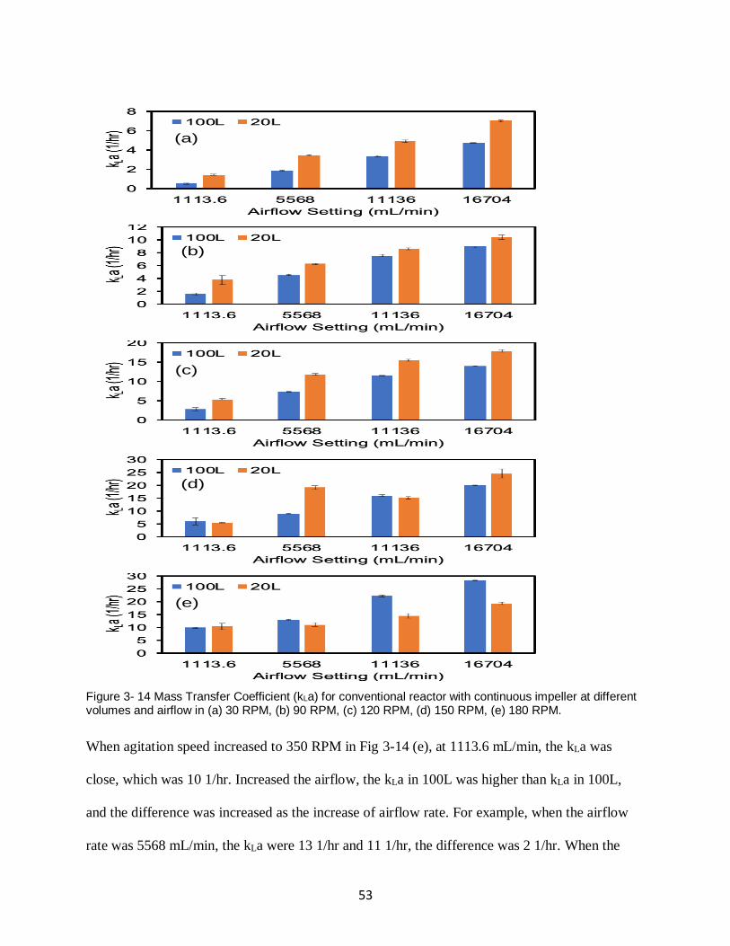
53
Figure 3- 14 Mass Transfer Coefficient (kLa) for conventional reactor with continuous impeller at different volumes and airflow in (a) 30 RPM, (b) 90 RPM, (c) 120 RPM, (d) 150 RPM, (e) 180 RPM.
When agitation speed increased to 350 RPM in Fig 3-14 (e), at 1113.6 mL/min, the kLa was
close, which was 10 1/hr. Increased the airflow, the kLa in 100L was higher than kLa in 100L,
and the difference was increased as the increase of airflow rate. For example, when the airflow
rate was 5568 mL/min, the kLa were 13 1/hr and 11 1/hr, the difference was 2 1/hr. When the
(e)
(d)
(c)
(b)
(a)
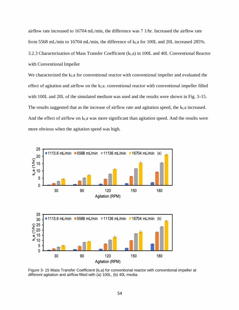
54
airflow rate increased to 16704 mL/min, the difference was 7 1/hr. Increased the airflow rate
from 5568 mL/min to 16704 mL/min, the difference of kLa for 100L and 20L increased 285%.
3.2.3 Characterization of Mass Transfer Coefficient (kLa) in 100L and 40L Conventional Reactor
with Conventional Impeller
We characterized the kLa for conventional reactor with conventional impeller and evaluated the
effect of agitation and airflow on the kLa. conventional reactor with conventional impeller filled
with 100L and 20L of the simulated medium was used and the results were shown in Fig. 3-15.
The results suggested that as the increase of airflow rate and agitation speed, the kLa increased.
And the effect of airflow on kLa was more significant than agitation speed. And the results were
more obvious when the agitation speed was high.
Figure 3- 15 Mass Transfer Coefficient (kLa) for conventional reactor with conventional impeller at different agitation and airflow filled with (a) 100L, (b) 40L media.
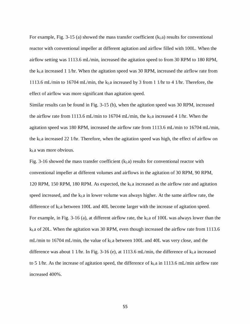
55
For example, Fig. 3-15 (a) showed the mass transfer coefficient (kLa) results for conventional
reactor with conventional impeller at different agitation and airflow filled with 100L. When the
airflow setting was 1113.6 mL/min, increased the agitation speed to from 30 RPM to 180 RPM,
the kLa increased 1 1/hr. When the agitation speed was 30 RPM, increased the airflow rate from
1113.6 mL/min to 16704 mL/min, the kLa increased by 3 from 1 1/hr to 4 1/hr. Therefore, the
effect of airflow was more significant than agitation speed.
Similar results can be found in Fig. 3-15 (b), when the agitation speed was 30 RPM, increased
the airflow rate from 1113.6 mL/min to 16704 mL/min, the kLa increased 4 1/hr. When the
agitation speed was 180 RPM, increased the airflow rate from 1113.6 mL/min to 16704 mL/min,
the kLa increased 22 1/hr. Therefore, when the agitation speed was high, the effect of airflow on
kLa was more obvious.
Fig. 3-16 showed the mass transfer coefficient (kLa) results for conventional reactor with
conventional impeller at different volumes and airflows in the agitation of 30 RPM, 90 RPM,
120 RPM, 150 RPM, 180 RPM. As expected, the kLa increased as the airflow rate and agitation
speed increased, and the kLa in lower volume was always higher. At the same airflow rate, the
difference of kLa between 100L and 40L become larger with the increase of agitation speed.
For example, in Fig. 3-16 (a), at different airflow rate, the kLa of 100L was always lower than the
kLa of 20L. When the agitation was 30 RPM, even though increased the airflow rate from 1113.6
mL/min to 16704 mL/min, the value of kLa between 100L and 40L was very close, and the
difference was about 1 1/hr. In Fig. 3-16 (e), at 1113.6 mL/min, the difference of kLa increased
to 5 1/hr. As the increase of agitation speed, the difference of kLa in 1113.6 mL/min airflow rate
increased 400%.
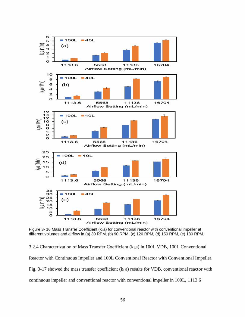
56
Figure 3- 16 Mass Transfer Coefficient (kLa) for conventional reactor with conventional impeller at different volumes and airflow in (a) 30 RPM, (b) 90 RPM, (c) 120 RPM, (d) 150 RPM, (e) 180 RPM.
3.2.4 Characterization of Mass Transfer Coefficient (kLa) in 100L VDB, 100L Conventional
Reactor with Continuous Impeller and 100L Conventional Reactor with Conventional Impeller.
Fig. 3-17 showed the mass transfer coefficient (kLa) results for VDB, conventional reactor with
continuous impeller and conventional reactor with conventional impeller in 100L, 1113.6
(e)
(d)
(c)
(b)
(a)
(a)
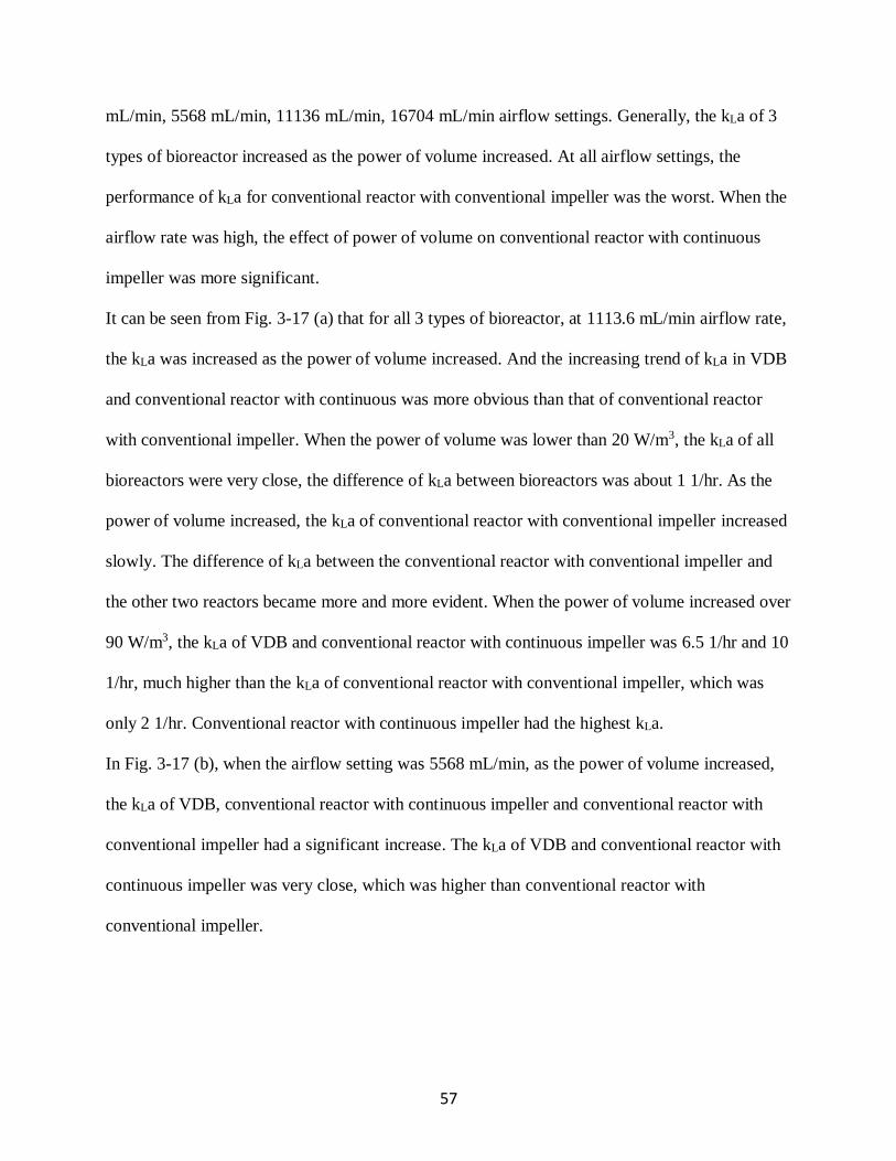
57
mL/min, 5568 mL/min, 11136 mL/min, 16704 mL/min airflow settings. Generally, the kLa of 3
types of bioreactor increased as the power of volume increased. At all airflow settings, the
performance of kLa for conventional reactor with conventional impeller was the worst. When the
airflow rate was high, the effect of power of volume on conventional reactor with continuous
impeller was more significant.
It can be seen from Fig. 3-17 (a) that for all 3 types of bioreactor, at 1113.6 mL/min airflow rate,
the kLa was increased as the power of volume increased. And the increasing trend of kLa in VDB
and conventional reactor with continuous was more obvious than that of conventional reactor
with conventional impeller. When the power of volume was lower than 20 W/m3, the kLa of all
bioreactors were very close, the difference of kLa between bioreactors was about 1 1/hr. As the
power of volume increased, the kLa of conventional reactor with conventional impeller increased
slowly. The difference of kLa between the conventional reactor with conventional impeller and
the other two reactors became more and more evident. When the power of volume increased over
90 W/m3, the kLa of VDB and conventional reactor with continuous impeller was 6.5 1/hr and 10
1/hr, much higher than the kLa of conventional reactor with conventional impeller, which was
only 2 1/hr. Conventional reactor with continuous impeller had the highest kLa.
In Fig. 3-17 (b), when the airflow setting was 5568 mL/min, as the power of volume increased,
the kLa of VDB, conventional reactor with continuous impeller and conventional reactor with
conventional impeller had a significant increase. The kLa of VDB and conventional reactor with
continuous impeller was very close, which was higher than conventional reactor with
conventional impeller.
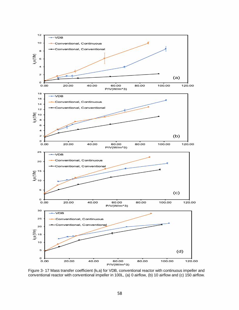
58
Figure 3- 17 Mass transfer coefficient (kLa) for VDB, conventional reactor with continuous impeller and conventional reactor with conventional impeller in 100L, (a) 0 airflow, (b) 10 airflow and (c) 150 airflow.
(d)
(c)
(b)
(a)
59
When the airflow increased to 11136 mL/min and 16704 mL/min in Fig. 3-17 (c) and Fig. 3-17
(d), as the increase of power of volume, the value of kLa increased. And the kLa of conventional
reactor with continuous impeller and conventional impeller had an evident increased when the
power of volume increased from 0 W/m3 to 20 W/m3. When the power of volume was higher
than 22 W/m3, it can be noticed that the kLa in conventional reactor with continuous impeller was
higher than the kLa in VDB, and the increasing rate was higher. Conventional reactor with
conventional impeller still had the lowest kLa.
Overall, as the increase of airflow rate, for all bioreactors, the kLa increased. And under any
condition of power of volume and airflow rate, VDB and conventional reactor with continuous
impeller always had a higher value of kLa. When the airflow rate was high, the power of volume
was lower than 20 W/m3, VDB had higher kLa than conventional reactor with continuous
impeller. As the effect of power of volume on conventional reactor with continuous impeller was
significant, the kLa in conventional reactor with continuous impeller was higher when the power
of volume was higher than 20 W/m3.
3.2.5 Characterization of Mass Transfer Coefficient (kLa) in 40L VDB and 40L Conventional
Reactor with Conventional Impeller.
Fig. 3-18 showed when VDB and conventional reactor with conventional impeller were filled
with 40L. As the increase of power of volume, the kLa of VDB and conventional reactor with
conventional impeller increased. And the kLa was very close in all power of volumes at different
airflow rates.
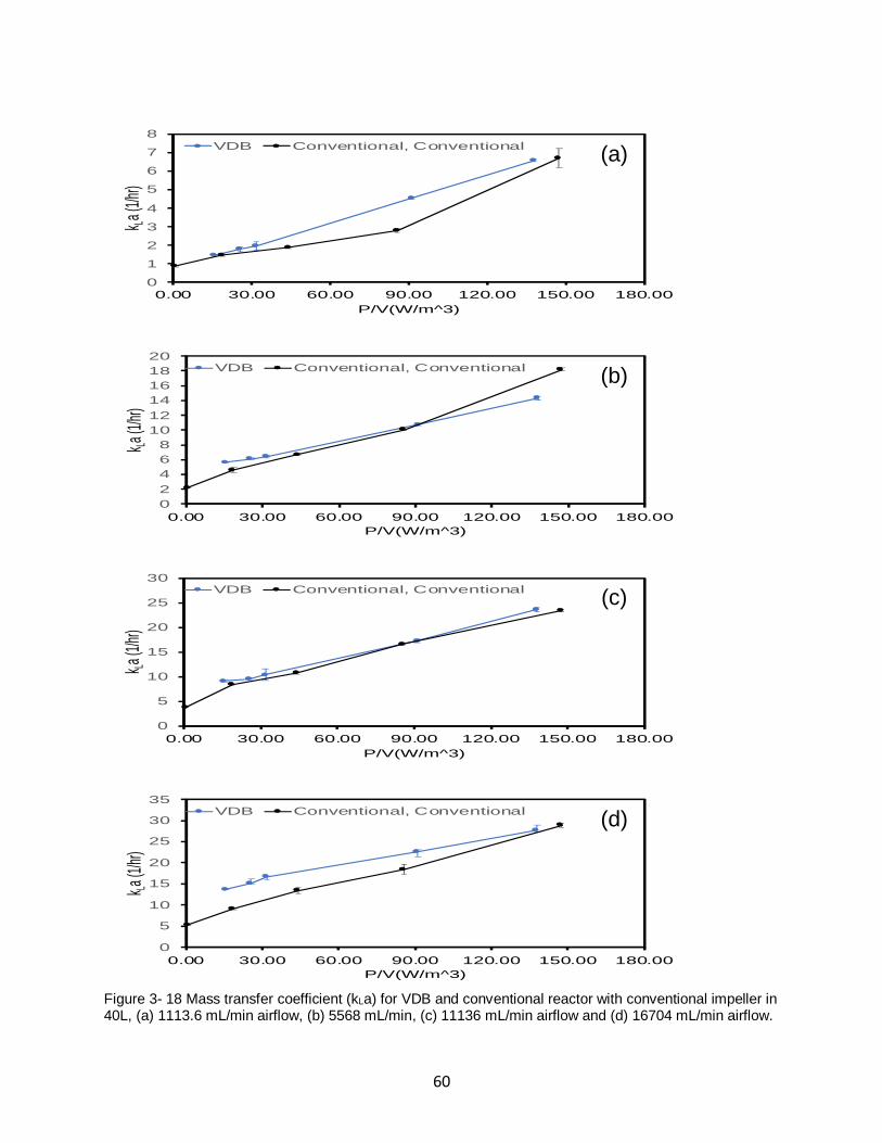
60
Figure 3- 18 Mass transfer coefficient (kLa) for VDB and conventional reactor with conventional impeller in 40L, (a) 1113.6 mL/min airflow, (b) 5568 mL/min, (c) 11136 mL/min airflow and (d) 16704 mL/min airflow.
0
1
2
3
4
5
6
7
8
0.00 30.00 60.00 90.00 120.00 150.00 180.00
k La (1
/hr)
P/V(W/m^3)
VDB Conventional, Conventional
0
2
4
6
8
10
12
14
16
18
20
0.00 30.00 60.00 90.00 120.00 150.00 180.00
k La (1
/hr)
P/V(W/m^3)
VDB Conventional, Conventional
0
5
10
15
20
25
30
0.00 30.00 60.00 90.00 120.00 150.00 180.00
k La (1
/hr)
P/V(W/m^3)
VDB Conventional, Conventional
0
5
10
15
20
25
30
35
0.00 30.00 60.00 90.00 120.00 150.00 180.00
k La (1
/hr)
P/V(W/m^3)
VDB Conventional, Conventional
(a)
(b)
(c)
(d)
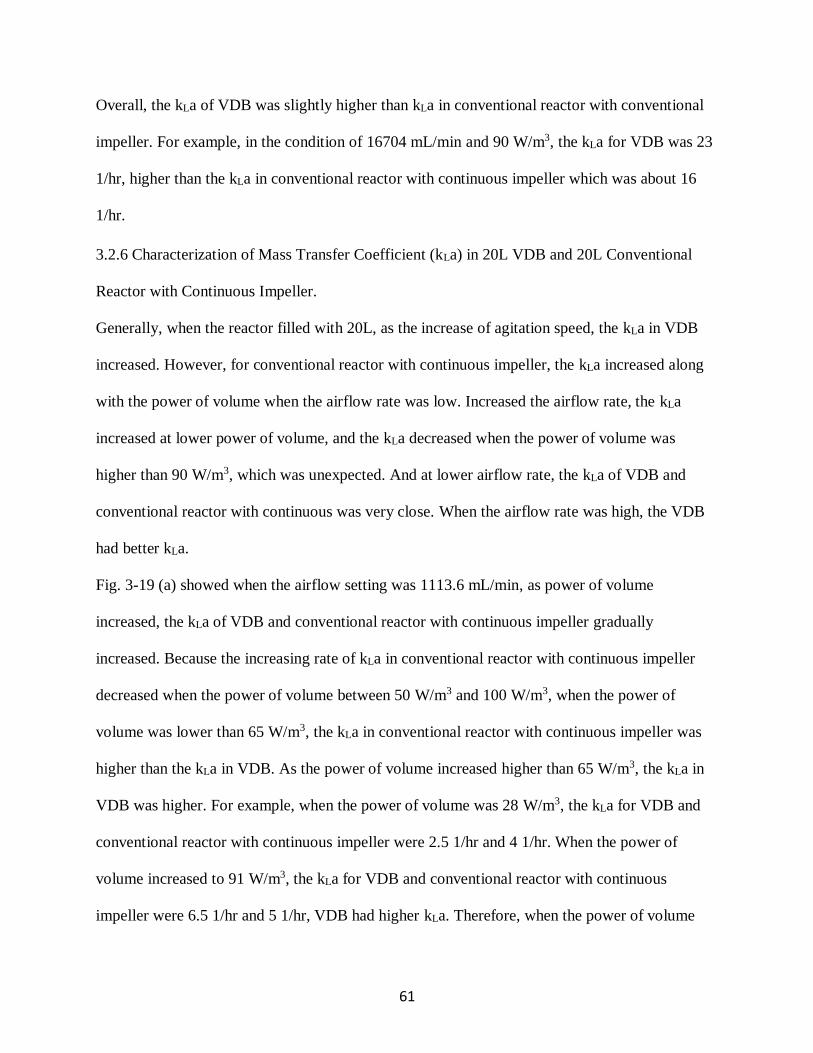
61
Overall, the kLa of VDB was slightly higher than kLa in conventional reactor with conventional
impeller. For example, in the condition of 16704 mL/min and 90 W/m3, the kLa for VDB was 23
1/hr, higher than the kLa in conventional reactor with continuous impeller which was about 16
1/hr.
3.2.6 Characterization of Mass Transfer Coefficient (kLa) in 20L VDB and 20L Conventional
Reactor with Continuous Impeller.
Generally, when the reactor filled with 20L, as the increase of agitation speed, the kLa in VDB
increased. However, for conventional reactor with continuous impeller, the kLa increased along
with the power of volume when the airflow rate was low. Increased the airflow rate, the kLa
increased at lower power of volume, and the kLa decreased when the power of volume was
higher than 90 W/m3, which was unexpected. And at lower airflow rate, the kLa of VDB and
conventional reactor with continuous was very close. When the airflow rate was high, the VDB
had better kLa.
Fig. 3-19 (a) showed when the airflow setting was 1113.6 mL/min, as power of volume
increased, the kLa of VDB and conventional reactor with continuous impeller gradually
increased. Because the increasing rate of kLa in conventional reactor with continuous impeller
decreased when the power of volume between 50 W/m3 and 100 W/m3, when the power of
volume was lower than 65 W/m3, the kLa in conventional reactor with continuous impeller was
higher than the kLa in VDB. As the power of volume increased higher than 65 W/m3, the kLa in
VDB was higher. For example, when the power of volume was 28 W/m3, the kLa for VDB and
conventional reactor with continuous impeller were 2.5 1/hr and 4 1/hr. When the power of
volume increased to 91 W/m3, the kLa for VDB and conventional reactor with continuous
impeller were 6.5 1/hr and 5 1/hr, VDB had higher kLa. Therefore, when the power of volume
62
was low, VDB had better value of kLa. When the power of volume was high, conventional
reactor with continuous impeller had better kLa.
Figure 3- 19 Mass transfer coefficient (kLa) for VDB and conventional reactor with continuous impeller in 20L, (a) 0 airflow, (b) 1113.6 mL/min airflow and (c) 16704 mL/min airflow.
0
2
4
6
8
10
12
14
0.00 30.00 60.00 90.00 120.00 150.00 180.00
k La(1/h
r)
P/V(W/m^3)
VDB Conventional, Continuous
0
5
10
15
20
25
0.00 30.00 60.00 90.00 120.00 150.00 180.00
k La(1/h
r)
P/V(W/m^3)
VDB Conventional, Continuous
0
5
10
15
20
25
30
35
0.00 30.00 60.00 90.00 120.00 150.00 180.00
k La(1/h
r)
P/V(W/m^3)
VDB Conventional, Continuous
0
5
10
15
20
25
30
35
40
0.00 30.00 60.00 90.00 120.00 150.00 180.00
k La(1/h
r)
P/V(W/m^3)
VDB Conventional, Continuous
(a)
(b)
(c)
(d)
63
Fig. 3-19 (b) showed when the power of volume was lower than 30 W/m3, the kLa of VDB and
conventional reactor with continuous impeller was close. Increased power of volume from 30
W/m3 to 90 W/m3, the value of kLa in conventional reactor with continuous impeller exceeded
the value of kLa in VDB, and the difference was about 5 1/hr at 90 W/m3. When power of
volume increased from 90 W/m3 to 140 W/m3, the kLa in conventional reactor with continuous
impeller significantly decreased from 19 1/hr to 11 1/hr. However, the kLa in VDB kept
increasing from 14 1/hr to 20 1/hr, and reached the highest kLa in VDB at 5568 mL/min. At 90
W/m3, the conventional reactor with continuous impeller reached the highest kLa.
Fig. 3-19 (c) showed at 11136 mL/min airflow rate, the kLa of VDB increased with the increase
of power of volume. The kLa of conventional reactor with continuous impeller increased at a
lower power of volume almost unchanged when the power of volume increased. And at any
power of volume, we can find the kLa of VDB was higher than the kLa of conventional reactor
with continuous impeller. When the power of volume was 15 W/m3, the kLa of VDB and
conventional reactor with continuous impeller were 16 1/hr and 7 1/hr, the difference was
evident. Increased power of volume to 50 W/m3, the kLa of two reactors were very close, which
was about 16 1/hr. While increasing power of volume, the kLa of VDB increased from 16 1/hr to
25 1/hr, and the kLa of conventional reactor with continuous impeller decreased slightly from 15
1/hr to 13 1/hr.
When the airflow setting was 16704 mL/min, the results showed in Fig. 3-19 (d). It can be seen
that the kLa of VDB is higher than conventional reactor with continuous impeller at all power of
volume, and the kLa increased with the increase of power of volume. When the power of volume
was lower than 30 W/m3, similar to Fig. 3-19 (c), the kLa of conventional reactor with continuous
impeller increased evidently. In continuing to increase power of volume to 90 W/m3, kLa still had
64
a slightly increase. However, when the power of volume went up from 90 W/m3 to 170 W/m3,
the kLa decreased from 24 1/hr to 19 1/hr.
Overall, the kLa of VDB increased at all airflow settings. When the airflow setting was 5568
mL/min, 11136 mL/min and 16704 mL/min, the kLa of conventional reactor with continuous
impeller increased first and then decreased with the increase of power of volume. And when the
airflow setting was 1113.6 mL/min or 5568 mL/min, the kLa of two bioreactors were very close,
when the airflow setting was 11136 mL/min or 16704 mL/min, the kLa of VDB had a significant
advantage than the kLa of conventional reactor with continuous impeller.
Chapter 4: Biosynthesis of Antimicrobial Peptides (AMPs)
4.1 Introduction
4.1.1 Antimicrobial Peptides (AMPs)
Antimicrobial peptides (AMPs) are part of the innate immune response found among all classes
of life, witch a molecular weight of about 2000 to 7000 and composed of 20 to 60 amino acids
(Bulet et al., 1999). Most of these peptides have the characteristics of thermal stability and
broad-spectrum antibacterial activities (Broekaert et al., 1997).
Since the discovery of antimicrobial peptides, a large number of studies have been conducted on
the mechanism of action of antimicrobial peptides. It is currently known that antimicrobial
peptides act by acting on bacterial cell membranes (Epand and Vogel, 1999; Sanders et al.,
2007). On this basis, a variety of models of the interaction of antimicrobial peptides and cell
membranes have been proposed. At present, it is generally believed that antimicrobial peptides
act on cell membranes to form transmembrane ion channels on the membrane, destroying the
integrity of the membrane, causing cell rupture, and thereby killing the cells (Chen, L. et al.,
2009). With the deepening of research work, it was found that some antibacterial peptides have a
65
strong killing effect on some fungi, protozoa, viruses and cancer cells. Because of the wide
biological activity, antibacterial peptide shows the great potential in medicine application
prospects to instead antibiotics in the future (Bahar and Ren, 2013).
Since bacterial resistance and emerging infectious diseases have become potential threats to
humans, the synthesis of antimicrobial peptides has become a promising focus area for antibiotic
research. However, antimicrobial peptides are minimal in animals. The production of
antimicrobial peptides from animal cells have a low yield, time-consuming, complicated process,
and high cost, and large-scale production cannot be achieved (Izadpanah and Gallo, 2005). This
has become the biggest obstacle restricting the entry of antimicrobial peptides into practical
applications. Therefore, how to obtain a large number of antibacterial peptides with better
antibacterial activity has always been the main content of the development and production of
antibacterial peptides.
Antimicrobial peptides can be synthesized by the method of chemical synthesis, such as glycyl
glycin (Fischer and Fourneau, 1906) and octadecapeptide (Fischer, 1907). However, the process
of chemical synthesis is complicated, the conditions are harsh, and the cost is high. In addition,
because there are many by-products in the reaction process, the product purification is
complicated. More and more studies have shown that, compared with the chemical synthesis
method, the use of genetic engineering technology is an effective method to develop and produce
antimicrobial peptides (Sablon et al., 2000). On the one hand, the antibacterial peptides obtained
through genetic engineering technology can be identified and developed as products; on the other
hand, compared with other methods, the genetic engineering method has the potential advantages
of large-scale production and low cost. And the development of molecular biology and DNA
66
recombination technology in recent years has also provided good technical support for the
genetic engineering of antimicrobial peptides (Ingram et al., 1987).
The traditional method for cellular production of proteins/peptides using recombinant DNA
technology has been attempted for the production of AMPs. The gene encoding for the target
protein/peptide is inserted into a host for the expression for the protein/peptide. E. coli
expression systems are the most common among all methods of genetically engineered bacteria
to produce antimicrobial peptides (Plückthun, 1991). The clear genetic background, mature
expression technology and rapid growth of bacteria make it widely used. This also enables the
expression of various types of antimicrobial peptides in E. coli. Studies have shown that the
expression level of general antimicrobial peptides in E. coli varies according to the type of
carrier and the type of antimicrobial peptide, and the expression yield of human antimicrobial
peptides is mostly high. For example, the compound antimicrobial peptide AL32-P113 and the
recombinant antimicrobial peptide UBI 18-35 achieved expression in E. coli, and obtained
considerable expression levels of 12.1 mg/L and 6 mg/L (Ashcheulova et al., 2018; Wanmakok
et al., 2018). At present, using E. coli as host cells to produce antimicrobial peptides is
developed.
However, because of the killing effect and small size of antimicrobial peptides, use E. coli as
host cells to produce antimicrobial peptides still have problems. There are many factors affecting
the production of antibacterial peptides in E. coli. For example, Fig 4-1 shows the protentional
problems by using E. coli to produce antimicrobial peptides. As shown in Fig 4-1(a), it is easy to
produce endotoxin, which will cause the antimicrobial peptides to easily cause "suicide" to the
host during the later expression process (Rosano and Ceccarelli, 2014). In other words, after the
host cell express the antimicrobial peptides, because of the killing effect of the antimicrobial
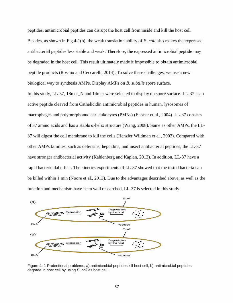
67
peptides, antimicrobial peptides can disrupt the host cell from inside and kill the host cell.
Besides, as shown in Fig 4-1(b), the weak translation ability of E. coli also makes the expressed
antibacterial peptides less stable and weak. Therefore, the expressed antimicrobial peptide may
be degraded in the host cell. This result ultimately made it impossible to obtain antimicrobial
peptide products (Rosano and Ceccarelli, 2014). To solve these challenges, we use a new
biological way to synthesis AMPs. Display AMPs on B. subtilis spore surface.
In this study, LL-37, 18mer_N and 14mer were selected to display on spore surface. LL-37 is an
active peptide cleaved from Cathelicidin antimicrobial peptides in human, lysosomes of
macrophages and polymorphonuclear leukocytes (PMNs) (Elssner et al., 2004). LL-37 consists
of 37 amino acids and has a stable α-helix structure (Wang, 2008). Same as other AMPs, the LL-
37 will digest the cell membrane to kill the cells (Henzler Wildman et al., 2003). Compared with
other AMPs families, such as defensins, hepcidins, and insect antibacterial peptides, the LL-37
have stronger antibacterial activity (Kahlenberg and Kaplan, 2013). In addition, LL-37 have a
rapid bactericidal effect. The kinetics experiments of LL-37 showed that the tested bacteria can
be killed within 1 min (Noore et al., 2013). Due to the advantages described above, as well as the
function and mechanism have been well researched, LL-37 is selected in this study.
Figure 4- 1 Protentional problems, a) antimicrobial peptides kill host cell, b) antimicrobial peptides degrade in host cell by using E. coli as host cell.
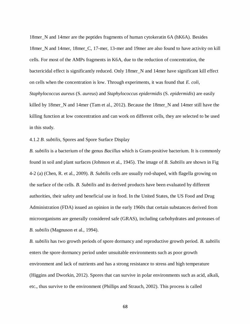
68
18mer_N and 14mer are the peptides fragments of human cytokeratin 6A (hK6A). Besides
18mer_N and 14mer, 18mer_C, 17-mer, 13-mer and 19mer are also found to have activity on kill
cells. For most of the AMPs fragments in K6A, due to the reduction of concentration, the
bactericidal effect is significantly reduced. Only 18mer_N and 14mer have significant kill effect
on cells when the concentration is low. Through experiments, it was found that E. coli,
Staphylococcus aureus (S. aureus) and Staphylococcus epidermidis (S. epidermidis) are easily
killed by 18mer_N and 14mer (Tam et al., 2012). Because the 18mer_N and 14mer still have the
killing function at low concentration and can work on different cells, they are selected to be used
in this study.
4.1.2 B. subtilis, Spores and Spore Surface Display
B. subtilis is a bacterium of the genus Bacillus which is Gram-positive bacterium. It is commonly
found in soil and plant surfaces (Johnson et al., 1945). The image of B. Subtilis are shown in Fig
4-2 (a) (Chen, R. et al., 2009). B. Subtilis cells are usually rod-shaped, with flagella growing on
the surface of the cells. B. Subtilis and its derived products have been evaluated by different
authorities, their safety and beneficial use in food. In the United States, the US Food and Drug
Administration (FDA) issued an opinion in the early 1960s that certain substances derived from
microorganisms are generally considered safe (GRAS), including carbohydrates and proteases of
B. subtilis (Magnuson et al., 1994).
B. subtilis has two growth periods of spore dormancy and reproductive growth period. B. subtilis
enters the spore dormancy period under unsuitable environments such as poor growth
environment and lack of nutrients and has a strong resistance to stress and high temperature
(Higgins and Dworkin, 2012). Spores that can survive in polar environments such as acid, alkali,
etc., thus survive to the environment (Phillips and Strauch, 2002). This process is called
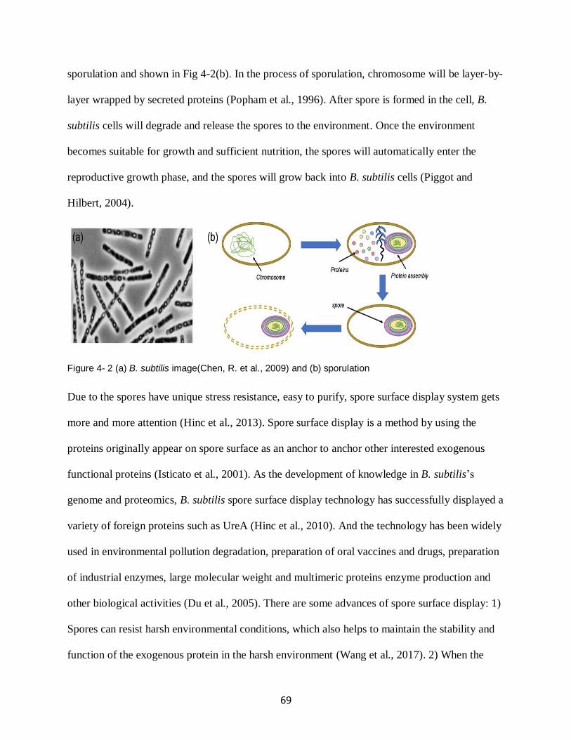
69
sporulation and shown in Fig 4-2(b). In the process of sporulation, chromosome will be layer-by-
layer wrapped by secreted proteins (Popham et al., 1996). After spore is formed in the cell, B.
subtilis cells will degrade and release the spores to the environment. Once the environment
becomes suitable for growth and sufficient nutrition, the spores will automatically enter the
reproductive growth phase, and the spores will grow back into B. subtilis cells (Piggot and
Hilbert, 2004).
Figure 4- 2 (a) B. subtilis image(Chen, R. et al., 2009) and (b) sporulation
Due to the spores have unique stress resistance, easy to purify, spore surface display system gets
more and more attention (Hinc et al., 2013). Spore surface display is a method by using the
proteins originally appear on spore surface as an anchor to anchor other interested exogenous
functional proteins (Isticato et al., 2001). As the development of knowledge in B. subtilis’s
genome and proteomics, B. subtilis spore surface display technology has successfully displayed a
variety of foreign proteins such as UreA (Hinc et al., 2010). And the technology has been widely
used in environmental pollution degradation, preparation of oral vaccines and drugs, preparation
of industrial enzymes, large molecular weight and multimeric proteins enzyme production and
other biological activities (Du et al., 2005). There are some advances of spore surface display: 1)
Spores can resist harsh environmental conditions, which also helps to maintain the stability and
function of the exogenous protein in the harsh environment (Wang et al., 2017). 2) When the
70
mother cell expresses the coat protein, the exogenous protein will also be expressed in the same
time. Naturally, the coat protein will appear on the surface of the spore, then the interested
protein will also be dragged to the surface of the spore, which avoid the interested protein cross
the cell membrane (Iwanicki et al., 2014). 3) Compared with other host cells such as E. coli,
displaying proteins on the surface of spores can avoid protein purification and protein separation,
which can reduce production costs, save time, and increase economic benefits (Isticato and
Ricca, 2016).
Figure 4- 3 (a) Wild type spore, (b) AMPs fused with coat protein gene sequence, c) engineered spore with AMPs on spore surface.
Fig 4-3 (a) shows the structure of wildtype spore. It can be seen that the spore is multilayers
structure, and the coat proteins are on spore surface (BAYLISS et al., 1981). In this study, we
selected CgeA or CotC as anchor protein from many coat proteins. As shown in Fig 4-3 (b), fuse
the AMPs on the N-terminal or C-terminal of cgeA or cotC. When the B. subtilis express CgeA
or CotC, originally, CgeA or CotC will appear on the spore surface. AMPs will be dragged to the
spore surface as well. Then we can get the engineered spore with AMPs on spore surface as
shown in Fig 4-3 (c). This process is called AMPs display on spore surface.
71
4.1.3 Intein
Intein is a sequence of amino acids present in the precursor protein (Perler et al., 1997). When
the precursor protein is converted into a mature protein, it is released from the precursor protein
by self-splicing, and the peptide chains at both ends are connected by peptide bonds (Mills and
Perler, 2005; Shemella et al., 2007). This process is the self-cutting of the protein. The first intein
was discovered in 1988 (Perler, 2002). They are distributed in the genomes of single-cell
eukaryotes, eukaryotes, archaebacteria, bacteriophages and viruses (Gogarten et al., 2002). The
types of Intein can be categorized into four classes: 1) Maxi-Intin, 2) Mini-Intein, 3) Alanine
Intein and 4) Trans-Splicing Intein. Maxi-inteins and mini-Intein are C-terminal and N-terminal
splicing domains, the difference is Maxi-inteins has an endonuclease domain, which does not
appear in mini-intein. Alanine intein can splicing in the splicing site which has alanine. In trans-
splicing intein, the intein can be spliced into two or more domains, then the domains will divide
into N-terminal and C-terminal (Shah et al., 2011).
The discovery of self-splicing mechanisms provides convenience for protein engineering,
especially in terms of protein purification, and is a pioneering breakthrough (Wood et al., 1999).
The uniqueness of the intein is its self-splicing function, which can connect two peptides with a
normal peptide bond, and then break down into N-terminal and C-terminal through the self-
splicing. Therefore, this characteristic of intein has a wide range of applications in metabolic
engineering, protein labeling, biomaterial construction, protein cyclization, and protein
purification. Due to the development of self-cleaving affinity tags, one of the main applications
of intein is for protein purification. Modified intein is fused to target protein and affinity tag.
Once the fusion is affinity-purified, intein can be incubated to splice target protein from the tag
and intein. After the target protein is separated from the intein and tag, a pure product can be
72
obtained. In this way, the purpose of protein purification is achieved. Intein can be used as
biosensors to detect protein-protein interactions also. Engineered split inteins are fused to the
target protein and reporter, respectively. An interaction between the target protein and reporter
brings the split intein fragments closely, leading to intein activation and then split from the target
protein. Based on this mechanism, Umezawa and co-workers designed several protein-protein
interaction biosensors using GFP and luciferase as reporters in single cell organisms and
transgenic animals. Besides, inteins are also used as biosensors to detect protease activity, small
molecules and protein-DNA interactions (Shah et al., 2011).
In this study, MXE GyrA intein (MXE) purchased from NEB (NEB #N6707) was used to
connect coat protein CotC and AMPs. MXE is a mini-intein has 198 amino acids from
Mycobacterium xenopi gyrA gene and have be modified to cleavage at its N-terminus (Kurpiers
and Mootz, 2008). MXE has been used to purify a wide range of target protein. We fused the
AMPs on the N-terminal of MXE, and fused cotC on the C-terminal of MXE, results in no extra
amino acids on the target protein (AMPs) after cleavage. AMPs can be cleaved and harvested
from spores. This method provides an idea for large scale production of yield ultra-pure AMPs
for practical applications.
4.2 Material and Method
4.2.1 Media and Solutions
Luria-Bertani (LB) media powder (tryptone 10g/L, yeast extract 5g/L, sodium chloride 10g/L),
1.5% agar and tryptose blood agar base (TBAB, tryptose 10g/L, beef extract 3g/L, sodium
chloride 5g/L, agar 15g/L) were purchased from Difco laboratories, VWR. Luria-Bertani (LB)
was used to culture Escherichia coli (E. coli) strains and Bacillus subtilis (B. subtilis) strains. LB
media powder and TBAB were made solution by adding deionized water. Solid LB media can
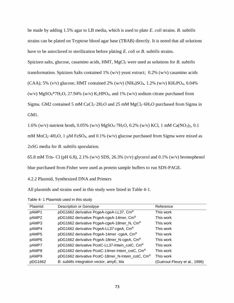
73
be made by adding 1.5% agar to LB media, which is used to plate E. coli strains. B. subtilis
strains can be plated on Tryptose blood agar base (TBAB) directly. It is noted that all solutions
have to be autoclaved to sterilization before plating E. coli or B. subtilis strains.
Spizizen salts, glucose, casamino acids, HMT, MgCl2 were used as solutions for B. subtilis
transformation. Spizizen Salts contained 1% (w/v) yeast extract; 0.2% (w/v) casamino acids
(CAA); 5% (v/v) glucose; HMT contained 2% (w/v) (NH4)SO4, 1.2% (w/v) KH2PO4, 0.04%
(w/v) MgSO4*7H2O, 27.94% (w/v) K2HPO4, and 1% (w/v) sodium citrate purchased from
Sigma. GM2 contained 5 mM CaCl2·2H2O and 25 mM MgCl2·6H2O purchased from Sigma in
GM1.
1.6% (w/v) nutrient broth, 0.05% (w/v) MgSO4·7H2O, 0.2% (w/v) KCl, 1 mM Ca(NO3)2, 0.1
mM MnCl2·4H2O, 1 μM FeSO4, and 0.1% (w/v) glucose purchased from Sigma were mixed as
2xSG media for B. subtilis sporulation.
65.8 mM Tris- Cl (pH 6.8), 2.1% (w/v) SDS, 26.3% (v/v) glycerol and 0.1% (w/v) bromophenol
blue purchased from Fisher were used as protein sample buffers to run SDS-PAGE.
4.2.2 Plasmid, Synthesized DNA and Primers
All plasmids and strains used in this study were listed in Table 4-1.
Table 4- 1 Plasmids used in this study
Plasmid Description or Genotpye Reference
pAMP1 pDG1662 derivative PcgeA-cgeA-LL37, CmR This work
pAMP2 pDG1662 derivative PcgeA-cgeA-14mer, CmR This work
pAMP3 pDG1662 derivative PcgeA-cgeA-18mer_N, CmR This work
pAMP4 pDG1662 derivative PcgeA-LL37-cgeA, CmR This work
pAMP5 pDG1662 derivative PcgeA-14mer -cgeA, CmR This work
pAMP6 pDG1662 derivative PcgeA-18mer_N-cgeA, CmR This work
pAMP7 pDG1662 derivative PcotC-LL37-Intein_cotC, CmR This work
pAMP8 pDG1662 derivative PcotC-14mer-Intein_cotC, CmR This work
pAMP9 pDG1662 derivative PcotC-18mer_N-Intein_cotC, CmR This work
pDG1662 B. subtilis integration vector, amyE, bla (Guérout-Fleury et al., 1996)
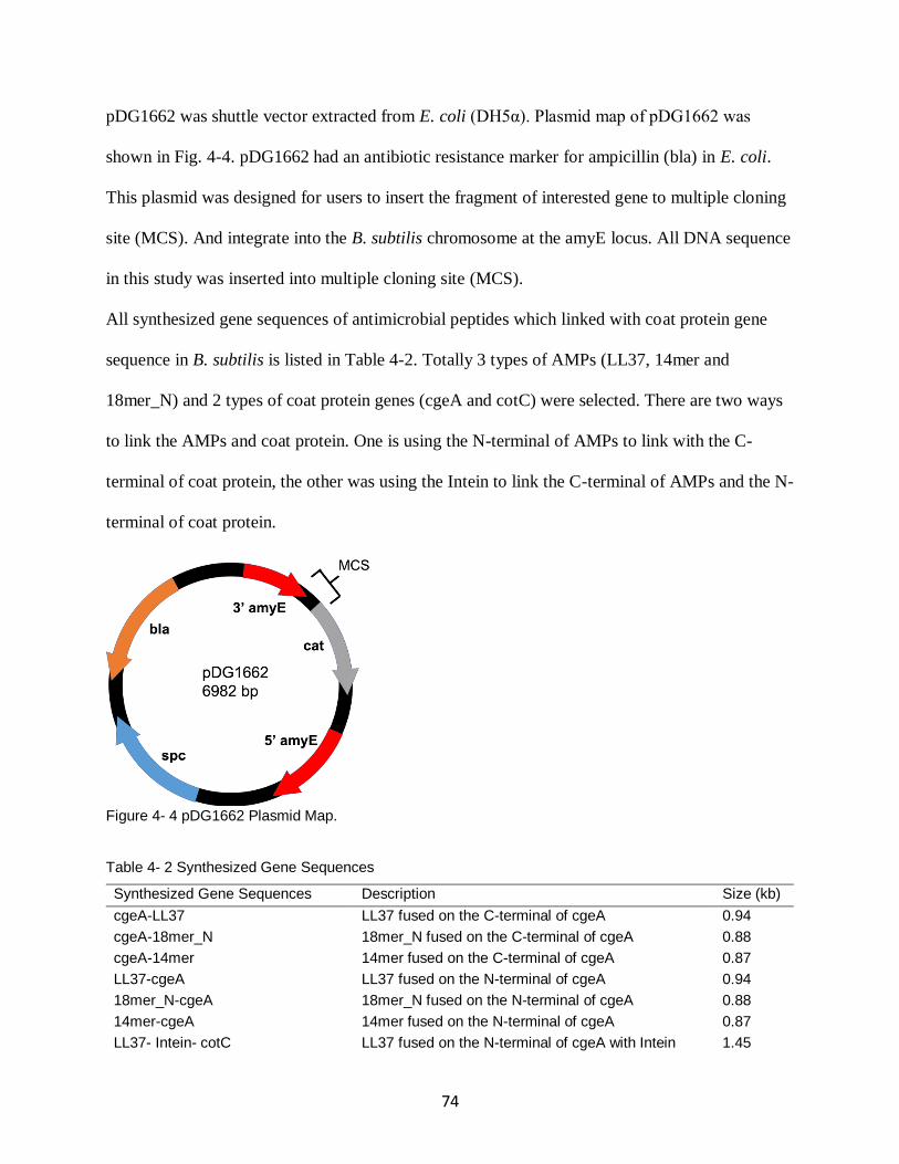
74
pDG1662 was shuttle vector extracted from E. coli (DH5α). Plasmid map of pDG1662 was
shown in Fig. 4-4. pDG1662 had an antibiotic resistance marker for ampicillin (bla) in E. coli.
This plasmid was designed for users to insert the fragment of interested gene to multiple cloning
site (MCS). And integrate into the B. subtilis chromosome at the amyE locus. All DNA sequence
in this study was inserted into multiple cloning site (MCS).
All synthesized gene sequences of antimicrobial peptides which linked with coat protein gene
sequence in B. subtilis is listed in Table 4-2. Totally 3 types of AMPs (LL37, 14mer and
18mer_N) and 2 types of coat protein genes (cgeA and cotC) were selected. There are two ways
to link the AMPs and coat protein. One is using the N-terminal of AMPs to link with the C-
terminal of coat protein, the other was using the Intein to link the C-terminal of AMPs and the N-
terminal of coat protein.
Figure 4- 4 pDG1662 Plasmid Map.
Table 4- 2 Synthesized Gene Sequences
Synthesized Gene Sequences Description Size (kb)
cgeA-LL37 LL37 fused on the C-terminal of cgeA 0.94
cgeA-18mer_N 18mer_N fused on the C-terminal of cgeA 0.88
cgeA-14mer 14mer fused on the C-terminal of cgeA 0.87
LL37-cgeA LL37 fused on the N-terminal of cgeA 0.94
18mer_N-cgeA 18mer_N fused on the N-terminal of cgeA 0.88
14mer-cgeA 14mer fused on the N-terminal of cgeA 0.87
LL37- Intein- cotC LL37 fused on the N-terminal of cgeA with Intein 1.45
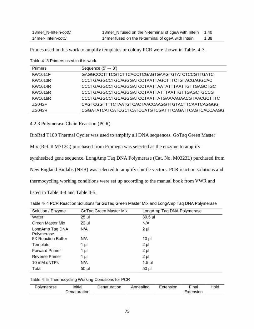
75
18mer_N-Intein-cotC 18mer_N fused on the N-terminal of cgeA with Intein 1.40
14mer- Intein-cotC 14mer fused on the N-terminal of cgeA with Intein 1.38
Primes used in this work to amplify templates or colony PCR were shown in Table. 4-3.
Table 4- 3 Primers used in this work.
Primers Sequence (5’ → 3’)
KW1611F GAGGCCCTTTCGTCTTCACCTCGAGTGAAGTGTATCTCCGTTGATC
KW1613R CCCTGAGGCCTGCAGGGATCCTAATTAGCTTTCTGTACGAGGCAC
KW1614R CCCTGAGGCCTGCAGGGATCCTAATTAATATTTAATTGTTGAGCTGC
KW1615R CCCTGAGGCCTGCAGGGATCCTAATTATTTAATTGTTGAGCTGCCG
KW1616R CCCTGAGGCCTGCAGGGATCCTAATTATGAAAAGAACGTAACGCTTTC
ZS042F CAGTCGGTTTTCTAATGTCACTAACCAAGGTTGTACTTCAATCAGGGG
ZS043R CGGATATCATCATCGCTCATCCATGTCGATTTCAGATTCAGTCACCAAGG
4.2.3 Polymerase Chain Reaction (PCR)
BioRad T100 Thermal Cycler was used to amplify all DNA sequences. GoTaq Green Master
Mix (Ref. # M712C) purchased from Promega was selected as the enzyme to amplify
synthesized gene sequence. LongAmp Taq DNA Polymerase (Cat. No. M0323L) purchased from
New England Biolabs (NEB) was selected to amplify shuttle vectors. PCR reaction solutions and
thermocycling working conditions were set up according to the manual book from VWR and
listed in Table 4-4 and Table 4-5.
Table 4- 4 PCR Reaction Solutions for GoTaq Green Master Mix and LongAmp Taq DNA Polymerase
Solution / Enzyme GoTaq Green Master Mix LongAmp Taq DNA Polymerase
Water 25 μl 30.5 μl
Green Master Mix 22 μl N/A
LongAmp Taq DNA Polymerase
N/A 2 μl
5X Reaction Buffer N/A 10 μl
Template 1 μl 2 μl
Forward Primer 1 μl 2 μl
Reverse Primer 1 μl 2 μl
10 mM dNTPs N/A 1.5 μl
Total 50 μl 50 μl
Table 4- 5 Thermocycling Working Conditions for PCR
Polymerase Initial Denaturation
Denaturation Annealing Extension Final Extension
Hold

76
GoTaq Green Master Mix
95°C, 2 mins
95°C, 30 seconds
5°C below the lowest primer Tm, 30 seconds
72°C, 1 min/kb
72°C, 5 mins
4°C
LongAmp Taq DNA Polymerase
94°C, 30 seconds
94°C, 30 seconds
5°C below the lowest primer Tm, 30 seconds
65°C, 50 sec/kb
65°C, 10 mins
4°C
4.2.4 Gel electrophoresis and DNA recovery
Gel electrophoresis was used to measure and purify DNA based on size. Agarose gel is made of
agarose with TAE buffer, 0.5 μg/ml ethidium bromide was used to stain agarose gel to visualize
DNA band and set in gel bed. Ladder purchased from NEB (Cat. No. N3232L) and samples
were loading in loading area and voltage was applied by using the PowerPac Basic unit from
BioRad for 120V, 30 mins to run sample. After running finished, gel was moved to UVP
Benchtop 2UV BioDoc-It Imaging System to be visualized at 365 nm.
DNA recovery was used to recover and purify DNA from agarose gel. Zymoclean Gel DNA
Recovery Kit (Cat. No. D4002) was used for gel recovery. Gel with DNA band was cut off and
move to autoclaved 1.5ml centrifuge tube. Add Agarose Dissolving Buffer (ADB) to the tube,
and the volume of ADB is 3 times than gel. Incubated tube at 50°C water bath until gel was fully
dissolved. Move liquid gel into Zymo-Spin column with collection tube, spined at 15000 RPM
for 30 seconds, discard filtrate. 200 μl DNA Wash Buffer was added, spined at 15000 RPM for
30 seconds again. Repeated this step and discard the filtrate. Moved Zymo-Spin column to a new
autoclaved 1.5ml centrifuge tube, 30 μl DNA Elution Buffer was added and spined at 15000
RPM for 30 seconds. Discarded Zymo-Spin column and stored DNA in centrifuge tube in -20°C
freezer.
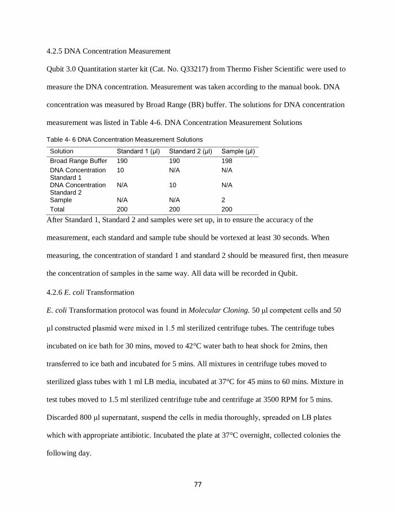
77
4.2.5 DNA Concentration Measurement
Qubit 3.0 Quantitation starter kit (Cat. No. Q33217) from Thermo Fisher Scientific were used to
measure the DNA concentration. Measurement was taken according to the manual book. DNA
concentration was measured by Broad Range (BR) buffer. The solutions for DNA concentration
measurement was listed in Table 4-6. DNA Concentration Measurement Solutions
Table 4- 6 DNA Concentration Measurement Solutions
Solution Standard 1 (μl) Standard 2 (μl) Sample (μl)
Broad Range Buffer 190 190 198
DNA Concentration Standard 1
10 N/A N/A
DNA Concentration Standard 2
N/A 10 N/A
Sample N/A N/A 2
Total 200 200 200
After Standard 1, Standard 2 and samples were set up, in to ensure the accuracy of the
measurement, each standard and sample tube should be vortexed at least 30 seconds. When
measuring, the concentration of standard 1 and standard 2 should be measured first, then measure
the concentration of samples in the same way. All data will be recorded in Qubit.
4.2.6 E. coli Transformation
E. coli Transformation protocol was found in Molecular Cloning. 50 μl competent cells and 50
μl constructed plasmid were mixed in 1.5 ml sterilized centrifuge tubes. The centrifuge tubes
incubated on ice bath for 30 mins, moved to 42°C water bath to heat shock for 2mins, then
transferred to ice bath and incubated for 5 mins. All mixtures in centrifuge tubes moved to
sterilized glass tubes with 1 ml LB media, incubated at 37°C for 45 mins to 60 mins. Mixture in
test tubes moved to 1.5 ml sterilized centrifuge tube and centrifuge at 3500 RPM for 5 mins.
Discarded 800 μl supernatant, suspend the cells in media thoroughly, spreaded on LB plates
which with appropriate antibiotic. Incubated the plate at 37°C overnight, collected colonies the
following day.
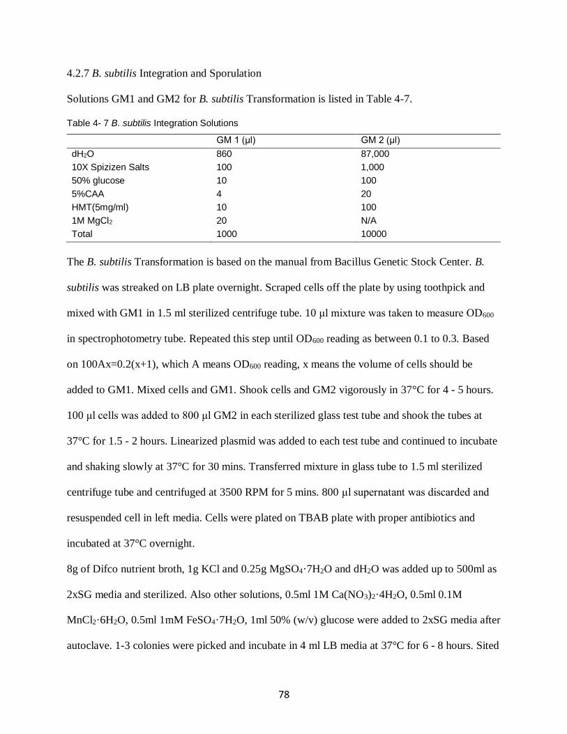
78
4.2.7 B. subtilis Integration and Sporulation
Solutions GM1 and GM2 for B. subtilis Transformation is listed in Table 4-7.
Table 4- 7 B. subtilis Integration Solutions
GM 1 (μl) GM 2 (μl)
dH2O 860 87,000
10X Spizizen Salts 100 1,000
50% glucose 10 100
5%CAA 4 20
HMT(5mg/ml) 10 100
1M MgCl2 20 N/A
Total 1000 10000
The B. subtilis Transformation is based on the manual from Bacillus Genetic Stock Center. B.
subtilis was streaked on LB plate overnight. Scraped cells off the plate by using toothpick and
mixed with GM1 in 1.5 ml sterilized centrifuge tube. 10 μl mixture was taken to measure OD600
in spectrophotometry tube. Repeated this step until OD600 reading as between 0.1 to 0.3. Based
on 100Ax=0.2(x+1), which A means OD600 reading, x means the volume of cells should be
added to GM1. Mixed cells and GM1. Shook cells and GM2 vigorously in 37°C for 4 - 5 hours.
100 μl cells was added to 800 μl GM2 in each sterilized glass test tube and shook the tubes at
37°C for 1.5 - 2 hours. Linearized plasmid was added to each test tube and continued to incubate
and shaking slowly at 37°C for 30 mins. Transferred mixture in glass tube to 1.5 ml sterilized
centrifuge tube and centrifuged at 3500 RPM for 5 mins. 800 μl supernatant was discarded and
resuspended cell in left media. Cells were plated on TBAB plate with proper antibiotics and
incubated at 37°C overnight.
8g of Difco nutrient broth, 1g KCl and 0.25g MgSO4·7H2O and dH2O was added up to 500ml as
2xSG media and sterilized. Also other solutions, 0.5ml 1M Ca(NO3)2·4H2O, 0.5ml 0.1M
MnCl2·6H2O, 0.5ml 1mM FeSO4·7H2O, 1ml 50% (w/v) glucose were added to 2xSG media after
autoclave. 1-3 colonies were picked and incubate in 4 ml LB media at 37°C for 6 - 8 hours. Sited
79
the solutions and 2xSG media at room temp for at least a couple of hours before starting the
culture. Transferred the LB media, 2xSG media to sterilized flask, incubated at 37°C with
shaking for 3 to 7 days. Transferred the spore culture to 50 ml sterilized centrifuge tubes and
centrifuged at 4000 rpm for 30-60 minutes at 4ºC. Carefully discarded the supernatant. Wash
spores by re-suspending the spores in sterile water, centrifuging for 30-60 minutes, and carefully
removing the supernatant. Repeated this steps for 5-8 times until supernatant was clear. Stored
spores in a small amount of sterile water at room temperature or 4ºC for short term use.
4.2.8 SDS-PAGE
Mini-PROTEAN TGX precast gels (Cat. No. 456-1094) purchased BioRad were used to run
Sodium Dodecyl Sulfate Polyacrylamide Gel Electrophoresis (SDS-PAGE). 65.8 mM Tris- Cl
(pH 6.8), 2.1% (w/v) SDS, 26.3% (v/v) glycerol and 0.1% (w/v) bromophenol blue were used as
buffer for samples. For each protein sample, 25 μl protein solution, 2 μl 2-mercaptoethanol and
23 μl freshly made buffer was mixed as working solutions. Set Mini-PROTEAN TGX precast
gel on BioRad Mini-PROTEAN Tetra System, running buffer which made with 2.5 mM Tris
base, 19.2 mM glycine, and 0.1% (w/v) SDS was added until the liquid level over loading area.
Working solutions and Benchmark His-tagged Protein Standard (Ref. No. LC5606) were loaded
into gel, running gel at 200V for 30 mins by using BioRad Mini-PROTEAN Tetra System. Gel
was removed after running finished, used SimplyBlue SafeStain purchased from Themo Fisher
Scientific (Cat. No. LC6060) to stain the gel and shaking slowly for 1 hour. Then moved the gel
to autoclaved water and let it stand still until protein bands can be visualized clearly.
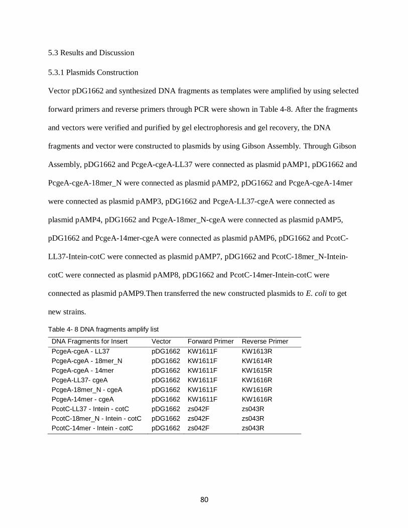
80
5.3 Results and Discussion
5.3.1 Plasmids Construction
Vector pDG1662 and synthesized DNA fragments as templates were amplified by using selected
forward primers and reverse primers through PCR were shown in Table 4-8. After the fragments
and vectors were verified and purified by gel electrophoresis and gel recovery, the DNA
fragments and vector were constructed to plasmids by using Gibson Assembly. Through Gibson
Assembly, pDG1662 and PcgeA-cgeA-LL37 were connected as plasmid pAMP1, pDG1662 and
PcgeA-cgeA-18mer_N were connected as plasmid pAMP2, pDG1662 and PcgeA-cgeA-14mer
were connected as plasmid pAMP3, pDG1662 and PcgeA-LL37-cgeA were connected as
plasmid pAMP4, pDG1662 and PcgeA-18mer_N-cgeA were connected as plasmid pAMP5,
pDG1662 and PcgeA-14mer-cgeA were connected as plasmid pAMP6, pDG1662 and PcotC-
LL37-Intein-cotC were connected as plasmid pAMP7, pDG1662 and PcotC-18mer_N-Intein-
cotC were connected as plasmid pAMP8, pDG1662 and PcotC-14mer-Intein-cotC were
connected as plasmid pAMP9.Then transferred the new constructed plasmids to E. coli to get
new strains.
Table 4- 8 DNA fragments amplify list
DNA Fragments for Insert Vector Forward Primer Reverse Primer
PcgeA-cgeA - LL37 pDG1662 KW1611F KW1613R
PcgeA-cgeA - 18mer_N pDG1662 KW1611F KW1614R
PcgeA-cgeA - 14mer pDG1662 KW1611F KW1615R
PcgeA-LL37- cgeA pDG1662 KW1611F KW1616R
PcgeA-18mer_N - cgeA pDG1662 KW1611F KW1616R
PcgeA-14mer - cgeA pDG1662 KW1611F KW1616R
PcotC-LL37 - Intein - cotC pDG1662 zs042F zs043R
PcotC-18mer_N - Intein - cotC pDG1662 zs042F zs043R
PcotC-14mer - Intein - cotC pDG1662 zs042F zs043R
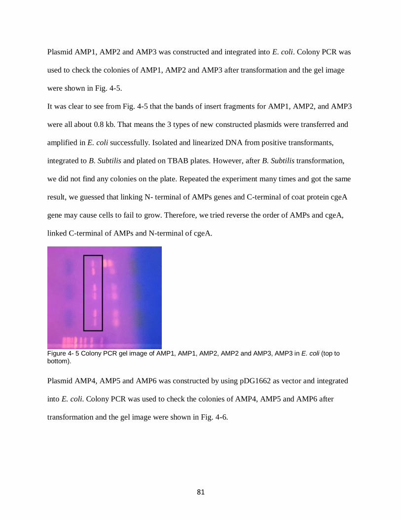
81
Plasmid AMP1, AMP2 and AMP3 was constructed and integrated into E. coli. Colony PCR was
used to check the colonies of AMP1, AMP2 and AMP3 after transformation and the gel image
were shown in Fig. 4-5.
It was clear to see from Fig. 4-5 that the bands of insert fragments for AMP1, AMP2, and AMP3
were all about 0.8 kb. That means the 3 types of new constructed plasmids were transferred and
amplified in E. coli successfully. Isolated and linearized DNA from positive transformants,
integrated to B. Subtilis and plated on TBAB plates. However, after B. Subtilis transformation,
we did not find any colonies on the plate. Repeated the experiment many times and got the same
result, we guessed that linking N- terminal of AMPs genes and C-terminal of coat protein cgeA
gene may cause cells to fail to grow. Therefore, we tried reverse the order of AMPs and cgeA,
linked C-terminal of AMPs and N-terminal of cgeA.
Figure 4- 5 Colony PCR gel image of AMP1, AMP1, AMP2, AMP2 and AMP3, AMP3 in E. coli (top to bottom).
Plasmid AMP4, AMP5 and AMP6 was constructed by using pDG1662 as vector and integrated
into E. coli. Colony PCR was used to check the colonies of AMP4, AMP5 and AMP6 after
transformation and the gel image were shown in Fig. 4-6.
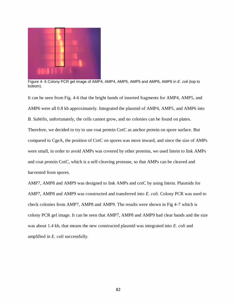
82
Figure 4- 6 Colony PCR gel image of AMP4, AMP4, AMP5, AMP5 and AMP6, AMP6 in E. coli (top to bottom).
It can be seen from Fig. 4-6 that the bright bands of inserted fragments for AMP4, AMP5, and
AMP6 were all 0.8 kb approximately. Integrated the plasmid of AMP4, AMP5, and AMP6 into
B. Subtilis, unfortunately, the cells cannot grow, and no colonies can be found on plates.
Therefore, we decided to try to use coat protein CotC as anchor protein on spore surface. But
compared to CgeA, the position of CotC on spores was more inward, and since the size of AMPs
were small, in order to avoid AMPs was covered by other proteins, we used Intein to link AMPs
and coat protein CotC, which is a self-cleaving protease, so that AMPs can be cleaved and
harvested from spores.
AMP7, AMP8 and AMP9 was designed to link AMPs and cotC by using Intein. Plasmids for
AMP7, AMP8 and AMP9 was constructed and transferred into E. coli. Colony PCR was used to
check colonies from AMP7, AMP8 and AMP9. The results were shown in Fig 4-7 which is
colony PCR gel image. It can be seen that AMP7, AMP8 and AMP9 had clear bands and the size
was about 1.4 kb, that means the new constructed plasmid was integrated into E. coli and
amplified in E. coli successfully.

83
Figure 4- 7 Colony PCR gel image of AMP7, AMP8 and AMP9 in E. coli (top to bottom).
Isolated and linearized DNA from positive transformants, integrated to B. Subtilis and plated on
TBAB plates. Fig. 4-8 showed that colonies were found on the TBAB plates which integrated by
using AMP8 and AMP9.
Figure 4- 8 Plate image of positive control, negative control, AMP8 and AMP9.
For each plate, colonies were selected randomly and did colony PCR. The results for colony
PCR were shown in Fig. 4-9 and indistinct bands can be found around 1.4 kb. That means the
plasmid of AMP8 and AMP9 had been integrated into B. Subtilis.
Figure 4- 9 Colony PCR gel image of AMP8 colony 1, 2, 3, 4 and AMP9 colony 1, 2 in B. Subtilis (top to bottom).
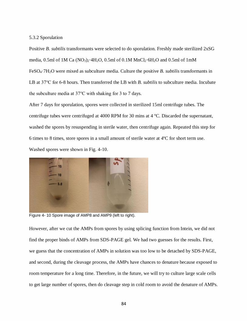
84
5.3.2 Sporulation
Positive B. subtilis transformants were selected to do sporulation. Freshly made sterilized 2xSG
media, 0.5ml of 1M Ca (NO3)2·4H2O, 0.5ml of 0.1M MnCl2·6H2O and 0.5ml of 1mM
FeSO4·7H2O were mixed as subculture media. Culture the positive B. subtilis transformants in
LB at 37℃ for 6-8 hours. Then transferred the LB with B. subtilis to subculture media. Incubate
the subculture media at 37℃ with shaking for 3 to 7 days.
After 7 days for sporulation, spores were collected in sterilized 15ml centrifuge tubes. The
centrifuge tubes were centrifuged at 4000 RPM for 30 mins at 4 ºC. Discarded the supernatant,
washed the spores by resuspending in sterile water, then centrifuge again. Repeated this step for
6 times to 8 times, store spores in a small amount of sterile water at 4ºC for short term use.
Washed spores were shown in Fig. 4-10.
Figure 4- 10 Spore image of AMP8 and AMP9 (left to right).
However, after we cut the AMPs from spores by using splicing function from Intein, we did not
find the proper binds of AMPs from SDS-PAGE gel. We had two guesses for the results. First,
we guess that the concentration of AMPs in solution was too low to be detached by SDS-PAGE,
and second, during the cleavage process, the AMPs have chances to denature because exposed to
room temperature for a long time. Therefore, in the future, we will try to culture large scale cells
to get large number of spores, then do cleavage step in cold room to avoid the denature of AMPs.
85
Concentrate AMPs solutions to obtain higher concentration products, then use SDS-PAGE to
detect the presence of AMPs.
86
LIST OF REFERENCE
Akkerman, I., Janssen, M., Rocha, J., Wijffels, R.H., 2002. Photobiological hydrogen production: photochemical efficiency and bioreactor design. International journal of hydrogen energy 27(11-12), 1195-1208. Altman, G.H., Lu, H.H., Horan, R.L., Calabro, T., Ryder, D., Kaplan, D.L., Stark, P., Martin, I., Richmond, J.C., Vunjak-Novakovic, G., 2002. Advanced bioreactor with controlled application of multi-dimensional strain for tissue engineering. J. Biomech. Eng. 124(6), 742-749. Asenjo, J.A., 1994. Bioreactor system design. CRC Press. Ashcheulova, D.O., Efimova, L.V., Lushchyk, A.Y., Yantsevich, A.V., Baikov, A.N., Pershina, A.G., 2018. Production of the recombinant antimicrobial peptide UBI18-35 in Escherichia coli. Protein Expression and Purification 143, 38-44. Bahar, A.A., Ren, D., 2013. Antimicrobial peptides. Pharmaceuticals 6(12), 1543-1575. BAYLISS, C.E., Waites, W., King, N., 1981. Resistance and structure of spores of Bacillus subtilis. Journal of Applied Bacteriology 50(2), 379-390. Boe, K., Angelidaki, I., 2009. Serial CSTR digester configuration for improving biogas production from manure. Water research 43(1), 166-172. Bredwell, M.D., Srivastava, P., Worden, R.M., 1999. Reactor design issues for synthesis‐gas fermentations. Biotechnology progress 15(5), 834-844. Broadley, S.T., Benton, P.R., 2010. Bioreactor jacket. Google Patents. Broekaert, W.F., Cammue, B.P., De Bolle, M.F., Thevissen, K., De Samblanx, G.W., Osborn, R.W., Nielson, K., 1997. Antimicrobial peptides from plants. Critical reviews in plant sciences 16(3), 297-323. Buchholz, R., Schügerl, K., 1979. Bubble column bioreactors. European journal of applied microbiology and biotechnology 6(4), 301-313. Bulet, P., Hetru, C., Dimarcq, J.-L., Hoffmann, D., 1999. Antimicrobial peptides in insects; structure and function. Developmental & Comparative Immunology 23(4-5), 329-344. Catapano, G., Czermak, P., Eibl, R., Eibl, D., Pörtner, R., 2009. Bioreactor design and scale-up, Cell and Tissue Reaction Engineering. Springer, pp. 173-259. Chen, C.-Y., Yeh, K.-L., Aisyah, R., Lee, D.-J., Chang, J.-S., 2011. Cultivation, photobioreactor design and harvesting of microalgae for biodiesel production: a critical review. Bioresource technology 102(1), 71-81. Chen, L., Jiao, Z.-H., Zheng, L.-S., Zhang, Y.-Y., Xie, S.-T., Wang, Z.-X., Wu, J.-W., 2009. Structural insight into the autoinhibition mechanism of AMP-activated protein kinase. Nature 459(7250), 1146-1149. Chen, R., Guttenplan, S.B., Blair, K.M., Kearns, D.B., 2009. Role of the σD-dependent autolysins in Bacillus subtilis population heterogeneity. Journal of bacteriology 191(18), 5775-5784. Chisti, Y., Kasper, M., Moo‐Young, M., 1990. Mass transfer in external‐loop airlift bioreactors using static mixers. The Canadian Journal of Chemical Engineering 68(1), 45-50. Damiani, A.L., Kim, M.H., Wang, J., 2014. An improved dynamic method to measure kLa in bioreactors. Biotechnology and bioengineering 111(10), 2120-2125. Daniell, H., Khan, M.S., Allison, L., 2002. Milestones in chloroplast genetic engineering: an environmentally friendly era in biotechnology. Trends in plant science 7(2), 84-91.
87
David, B., Dore, E., Jaffrin, M., Legallais, C., 2004. Mass transfers in a fluidized bed bioreactor using alginate beads for a future bioartificial liver. The International journal of artificial organs 27(4), 284-293. Du, C., Chan, W.C., McKeithan, T.W., Nickerson, K.W., 2005. Surface display of recombinant proteins on Bacillus thuringiensis spores. Applied and environmental microbiology 71(6), 3337-3341. Dutil, F., 2003. Photobioreactor. Google Patents. Elssner, A., Duncan, M., Gavrilin, M., Wewers, M.D., 2004. A novel P2X7 receptor activator, the human cathelicidin-derived peptide LL37, induces IL-1β processing and release. The Journal of Immunology 172(8), 4987-4994. Epand, R.M., Vogel, H.J., 1999. Diversity of antimicrobial peptides and their mechanisms of action. Biochimica et Biophysica Acta (BBA)-Biomembranes 1462(1-2), 11-28. Fischer, E., 1907. Synthetical chemistry in its relation to biology. Chemical Society. Fischer, E., Fourneau, E., 1906. Ueber einige derivate des glykocolls, Untersuchungen über Aminosäuren, Polypeptide und Proteïne (1899–1906). Springer, pp. 279-289. Fradette, S., Ruel, J., 2009. Process and a plant for recycling carbon dioxide emissions from power plants into useful carbonated species. Google Patents. Galaction, A.-I., Cascaval, D., Oniscu, C., Turnea, M., 2004. Prediction of oxygen mass transfer coefficients in stirred bioreactors for bacteria, yeasts and fungus broths. Biochemical Engineering Journal 20(1), 85-94. Garcia-Ochoa, F., Gomez, E., 2009. Bioreactor scale-up and oxygen transfer rate in microbial processes: an overview. Biotechnology advances 27(2), 153-176. Gill, N., Appleton, M., Baganz, F., Lye, G., 2008. Quantification of power consumption and oxygen transfer characteristics of a stirred miniature bioreactor for predictive fermentation scale‐up. Biotechnology and bioengineering 100(6), 1144-1155. Gogarten, J.P., Senejani, A.G., Zhaxybayeva, O., Olendzenski, L., Hilario, E., 2002. Inteins: structure, function, and evolution. Annual Reviews in Microbiology 56(1), 263-287. Gogate, P.R., Pandit, A.B., 1999. Survey of measurement techniques for gas–liquid mass transfer coefficient in bioreactors. Biochemical engineering journal 4(1), 7-15. Guérout-Fleury, A.-M., Frandsen, N., Stragier, P., 1996. Plasmids for ectopic integration in Bacillus subtilis. Gene 180(1-2), 57-61. Guo, H., Zhou, J., Su, J., Zhang, Z., 2005. Integration of nitrification and denitrification in airlift bioreactor. Biochemical Engineering Journal 23(1), 57-62. Handa, A., Emery, A., Spier, R., 1987. On the evaluation of gas-liquid interfacial effects on hybridoma viability in bubble column bioreactors. Developments in biological standardization 66, 241-253. Heck, W.W., Philbeck, R.B., Dunning, J.A., 1978. A continuous stirred tank reactor (CSTR) system for exposing plants to gaseous air contaminants: principles, specifications, construction, and operation. Department of Agriculture, Agricultural Research Service, Southern Region. Henzler Wildman, K.A., Lee, D.-K., Ramamoorthy, A., 2003. Mechanism of lipid bilayer disruption by the human antimicrobial peptide, LL-37. Biochemistry 42(21), 6545-6558. Higgins, D., Dworkin, J., 2012. Recent progress in Bacillus subtilis sporulation. FEMS microbiology reviews 36(1), 131-148.
88
Hinc, K., Isticato, R., Dembek, M., Karczewska, J., Iwanicki, A., Peszyńska-Sularz, G., De Felice, M., Obuchowski, M., Ricca, E., 2010. Expression and display of UreA of Helicobacter acinonychis on the surface of Bacillus subtilis spores. Microbial cell factories 9(1), 2. Hinc, K., Iwanicki, A., Obuchowski, M., 2013. New stable anchor protein and peptide linker suitable for successful spore surface display in B. subtilis. Microbial cell factories 12(1), 22. Horiuchi, J.-I., Ohba, I., Tada, K., Kobayashi, M., Kanno, T., Kishimoto, M., 2003. Effective cell harvesting of the halotolerant microalga Dunaliella tertiolecta with pH control. Journal of bioscience and bioengineering 95(4), 412-415. Hosseini, M., Shojaosadati, S.A., Towfighi, J., 2003. Application of a bubble-column reactor for the production of a single-cell protein from cheese whey. Industrial & engineering chemistry research 42(4), 764-766. Ingram, L., Conway, T., Clark, D., Sewell, G., Preston, J., 1987. Genetic engineering of ethanol production in Escherichia coli. Applied and Environmental Microbiology 53(10), 2420-2425. Isticato, R., Cangiano, G., Tran, H.T., Ciabattini, A., Medaglini, D., Oggioni, M.R., De Felice, M., Pozzi, G., Ricca, E., 2001. Surface display of recombinant proteins on Bacillus subtilis spores. Journal of Bacteriology 183(21), 6294-6301. Isticato, R., Ricca, E., 2016. Spore surface display. The Bacterial Spore: From Molecules to Systems, 349-366. Iwanicki, A., Piątek, I., Stasiłojć, M., Grela, A., Łęga, T., Obuchowski, M., Hinc, K., 2014. A system of vectors for Bacillus subtilis spore surface display. Microbial cell factories 13(1), 30. Izadpanah, A., Gallo, R.L., 2005. Antimicrobial peptides. Journal of the American Academy of Dermatology 52(3), 381-390. Johnson, B.A., Anker, H., Meleney, F.L., 1945. Bacitracin: a new antibiotic produced by a member of the B. subtilis group. Science 102(2650), 376-377. Kahlenberg, J.M., Kaplan, M.J., 2013. Little peptide, big effects: the role of LL-37 in inflammation and autoimmune disease. The Journal of Immunology 191(10), 4895-4901. Kawase, Y., Halard, B., Moo‐Young, M., 1992. Liquid‐phase mass transfer coefficients in bioreactors. Biotechnology and bioengineering 39(11), 1133-1140. Kim, J., Kim, K., Ye, H., Lee, E., Shin, C., McCarty, P.L., Bae, J., 2011. Anaerobic fluidized bed membrane bioreactor for wastewater treatment. Environmental science & technology 45(2), 576-581. Kim, S., Hahn, E., Paek, K., Murthy, H., 2002. Application of bioreactor culture for large scale production of Chrysanthemum transplants, XXVI International Horticultural Congress: Biotechnology in Horticultural Crop Improvement: Achievements, Opportunities and 625. pp. 187-191. Kunas, K.T., Papoutsakis, E.T., 1990. Damage mechanisms of suspended animal cells in agitated bioreactors with and without bubble entrainment. Biotechnology and bioengineering 36(5), 476-483. Kurpiers, T., Mootz, H.D., 2008. Site‐Specific Chemical Modification of Proteins with a Prelabelled Cysteine Tag Using the Artificially Split Mxe GyrA Intein. ChemBioChem 9(14), 2317-2325. Lee, S., Ibey, B.L., Coté, G.L., Pishko, M.V., 2008. Measurement of pH and dissolved oxygen within cell culture media using a hydrogel microarray sensor. Sensors and Actuators B: Chemical 128(2), 388-398.
89
Lee, S.Y., 1996. High cell-density culture of Escherichia coli. Trends in biotechnology 14(3), 98-105. Leite, J.A., Fernandes, B.S., Pozzi, E., Barboza, M., Zaiat, M., 2008. Application of an anaerobic packed-bed bioreactor for the production of hydrogen and organic acids. International Journal of Hydrogen Energy 33(2), 579-586. Linek, V., Beneš, P., Vacek, V., 1989. Dynamic pressure method for kla measurement in large‐scale bioreactors. Biotechnology and bioengineering 33(11), 1406-1412. Liu, C.-C., Wu, S.-C., Wu, S.-R., Lin, H.-Y., Guo, M.-S., Hu, A.Y.-C., Chow, Y.-H., Chiang, J.-R., Shieh, D.-B., Chong, P., 2018. Enhancing enterovirus A71 vaccine production yield by microcarrier profusion bioreactor culture. Vaccine 36(22), 3134-3139. Logan, B.E., LaPoint, D., 2002. Treatment of perchlorate-and nitrate-contaminated groundwater in an autotrophic, gas phase, packed-bed bioreactor. Water Research 36(14), 3647-3653. Lu, G.Z., Gray, M.R., Thompson, B.G., 1995. Cell culture bioreactor. Google Patents. Luo, H.-P., Al-Dahhan, M.H., 2010. Local gas holdup in a draft tube airlift bioreactor. Chemical engineering science 65(15), 4503-4510. Magnuson, R., Solomon, J., Grossman, A.D., 1994. Biochemical and genetic characterization of a competence pheromone from B. subtilis. Cell 77(2), 207-216. Mahmood, K.A., Wilkinson, S.J., Zimmerman, W.B., 2015. Airlift bioreactor for biological applications with microbubble mediated transport processes. Chemical Engineering Science 137, 243-253. Mantell, S.H., Matthews, J., McKee, R., 1985. Principles of plant biotechnology: an introduction to genetic engineering in plants. Blackwell Scientific Publications. Merchuk, J., Ben-Zvi, S., Niranjan, K., 1994. Why use bubble-column bioreactors? Trends in biotechnology 12(12), 501-511. Mills, K.V., Perler, F.B., 2005. The mechanism of intein-mediated protein splicing: variations on a theme. Protein and peptide letters 12(8), 751-755. Mohaisen, A., Yun, A., Kim, Y., 2010. Measuring the mixing time of social graphs, Proceedings of the 10th ACM SIGCOMM conference on Internet measurement. pp. 383-389. Molina, E., Fernández, J., Acién, F., Chisti, Y., 2001. Tubular photobioreactor design for algal cultures. Journal of biotechnology 92(2), 113-131. Mousavi, S.M., Jafari, A., Yaghmaei, S., Vossoughi, M., Turunen, I., 2008. Experiments and CFD simulation of ferrous biooxidation in a bubble column bioreactor. Computers & Chemical Engineering 32(8), 1681-1688. Nagel, F.J.J., Tramper, J., Bakker, M.S., Rinzema, A., 2001. Temperature control in a continuously mixed bioreactor for solid‐state fermentation. Biotechnology and Bioengineering 72(2), 219-230. Noore, J., Noore, A., Li, B., 2013. Cationic antimicrobial peptide LL-37 is effective against both extra-and intracellular Staphylococcus aureus. Antimicrobial agents and chemotherapy 57(3), 1283-1290. Özbek, B., Gayik, S., 2001. The studies on the oxygen mass transfer coefficient in a bioreactor. Process Biochemistry 36(8-9), 729-741. Park, S., Stephanopoulos, G., 1993. Packed bed bioreactor with porous ceramic beads for animal cell culture. Biotechnology and bioengineering 41(1), 25-34. Perler, F.B., 2002. InBase: the intein database. Nucleic acids research 30(1), 383-384.
90
Perler, F.B., Olsen, G.J., Adam, E., 1997. Compilation and analysis of intein sequences. Nucleic acids research 25(6), 1087-1093. Petersen, L.A., Villadsen, J., Jørgensen, S.B., Gernaey, K.V., 2017. Mixing and mass transfer in a pilot scale U‐loop bioreactor. Biotechnology and bioengineering 114(2), 344-354. Phillips, Z., Strauch, M., 2002. Bacillus subtilis sporulation and stationary phase gene expression. Cellular and Molecular Life Sciences CMLS 59(3), 392-402. Piggot, P.J., Hilbert, D.W., 2004. Sporulation of Bacillus subtilis. Current opinion in microbiology 7(6), 579-586. Plückthun, A., 1991. Antibody engineering: advances from the use of Escherichia coli expression systems. Bio/technology 9(6), 545-551. Polli, M., Di Stanislao, M., Bagatin, R., Bakr, E.A., Masi, M., 2002. Bubble size distribution in the sparger region of bubble columns. chemical Engineering science 57(1), 197-205. Popham, D.L., Helin, J., Costello, C.E., Setlow, P., 1996. Analysis of the peptidoglycan structure of Bacillus subtilis endospores. Journal of bacteriology 178(22), 6451-6458. Puskeiler, R., Weuster-Botz, D., 2005. Combined sulfite method for the measurement of the oxygen transfer coefficient kLa in bioreactors. Journal of biotechnology 120(4), 430-438. Rodriguez, G., Weheliye, W., Anderlei, T., Micheletti, M., Yianneskis, M., Ducci, A., 2013. Mixing time and kinetic energy measurements in a shaken cylindrical bioreactor. Chemical Engineering Research and Design 91(11), 2084-2097. Rosano, G.L., Ceccarelli, E.A., 2014. Recombinant protein expression in Escherichia coli: advances and challenges. Frontiers in microbiology 5, 172. Sablon, E., Contreras, B., Vandamme, E., 2000. Antimicrobial peptides of lactic acid bacteria: mode of action, genetics and biosynthesis, New Products and New Areas of Bioprocess Engineering. Springer, pp. 21-60. Sanders, M.J., Grondin, P.O., Hegarty, B.D., Snowden, M.A., Carling, D., 2007. Investigating the mechanism for AMP activation of the AMP-activated protein kinase cascade. Biochemical Journal 403(1), 139-148. Schügerl, K., Lücke, J., Oels, U., 1977. Bubble column bioreactors, Advances in Biochemical Engineering, Volume 7. Springer, pp. 1-84. Shah, N.H., Vila‐Perelló, M., Muir, T.W., 2011. Kinetic control of one‐pot trans‐splicing reactions by using a wild‐type and designed split intein. Angewandte Chemie International Edition 50(29), 6511-6515. Shemella, P., Pereira, B., Zhang, Y., Van Roey, P., Belfort, G., Garde, S., Nayak, S.K., 2007. Mechanism for intein C-terminal cleavage: a proposal from quantum mechanical calculations. Biophysical journal 92(3), 847-853. Simutis, R., Lübbert, A., 2015. Bioreactor control improves bioprocess performance. Biotechnology journal 10(8), 1115-1130. Singh, R., Sharma, S., 2012. Development of suitable photobioreactor for algae production–A review. Renewable and Sustainable Energy Reviews 16(4), 2347-2353. Spier, M.R., Vandenberghe, L., Medeiros, A.B.P., Soccol, C.R., 2011. Application of different types of bioreactors in bioprocesses. Bioreactors: design, properties and applications. Nova Science Publishers Inc: New York, 55-90. Suh, I.S., Lee, C.-G., 2003. Photobioreactor engineering: design and performance. Biotechnology and bioprocess engineering 8(6), 313.
91
Tam, C., Mun, J.J., Evans, D.J., Fleiszig, S.M., 2012. Cytokeratins mediate epithelial innate defense through their antimicrobial properties. The Journal of clinical investigation 122(10), 3665-3677. Tang, W.-T., Wisecarver, K., Fan, L.-S., 1987. Dynamics of a draft tube gas—liquid—solid fluidized bed bioreactor for phenol degradation. Chemical engineering science 42(9), 2123-2134. Trambouze, P., Piret, E.L., 1959. Continuous stirred tank reactors: Designs for maximum conversions of raw material to desired product. Homogeneous reactions. AIChE Journal 5(3), 384-390. Tunac, J., 1991. Fermentor/bioreactor systems having high aeration capacity. Google Patents. Van't Riet, K., Tramper, J., 1991. Basic bioreactor design. CRC press. Wang, G., 2008. Structures of human host defense cathelicidin LL-37 and its smallest antimicrobial peptide KR-12 in lipid micelles. Journal of Biological Chemistry 283(47), 32637-32643. Wang, H., Wang, Y., Yang, R., 2017. Recent progress in Bacillus subtilis spore-surface display: concept, progress, and future. Applied microbiology and biotechnology 101(3), 933-949. Wang, M.D., Yang, M., Huzel, N., Butler, M., 2002. Erythropoietin production from CHO cells grown by continuous culture in a fluidized‐bed bioreactor. Biotechnology and bioengineering 77(2), 194-203. Wang, S.J., Zhong, J.J., 1996. A novel centrifugal impeller bioreactor. II. Oxygen transfer and power consumption. Biotechnology and bioengineering 51(5), 520-527. Wanmakok, M., Orrapin, S., Intorasoot, A., Intorasoot, S., 2018. Expression in Escherichia coli of novel recombinant hybrid antimicrobial peptide AL32-P113 with enhanced antimicrobial activity in vitro. Gene 671, 1-9. Warnock, J.N., Al‐Rubeai, M., 2006. Bioreactor systems for the production of biopharmaceuticals from animal cells. Biotechnology and applied biochemistry 45(1), 1-12. Weissman, J.C., Goebel, R.P., Benemann, J.R., 1988. Photobioreactor design: mixing, carbon utilization, and oxygen accumulation. Biotechnology and bioengineering 31(4), 336-344. Wood, D.W., Wu, W., Belfort, G., Derbyshire, V., Belfort, M., 1999. A genetic system yields self-cleaving inteins for bioseparations. Nature biotechnology 17(9), 889-892. Wu, F., Dunkelman, N., Peterson, A., Davisson, T., de La Torre, R., Jain, D., 1999. Bioreactor development for tissue‐engineered cartilage. Annals of the New York Academy of Sciences 875(1), 405-411. Yen, H.-W., Liu, Y.X., 2014. Application of airlift bioreactor for the cultivation of aerobic oleaginous yeast Rhodotorula glutinis with different aeration rates. Journal of bioscience and bioengineering 118(2), 195-198. Young, M.A., Carbonell, R.G., Ollis, D.F., 1991. Airlift bioreactors: Analysis of local two‐phase hydrodynamics. AIChE journal 37(3), 403-428.