CHARACTERISTIC GENERA OF CLOSED ORIENTABLE

3-MANIFOLDS

AKIO KAWAUCHI

Osaka City University Advanced Mathematical Institute

Sugimoto, Sumiyoshi-ku, Osaka 558-8585, Japan

kawauchi@sci.osaka-cu.ac.jp

ABSTRACT

A complete invariant defined for (closed connected orientable) 3-manifoldsis an invariant defined for the 3-manifolds such that any two 3-manifolds withthe same invariant are homeomorphic. Further, if the 3-manifold itself canbe reconstructed from the data of the complete invariant, then it is calleda characteristic invariant defined for the 3-manifolds. In a previous work, acharacteristic lattice point invariant defined for the 3-manifolds was constructedby using an embedding of the prime links into the set of lattice points. Inthis paper, a characteristic rational invariant defined for the 3-manifolds calledthe characteristic genus defined for the 3-manifolds is constructed by using anembedding of a set of lattice points called the PDelta set into the set of rationalnumbers. The characteristic genus defined for the 3-manifolds is also comparedwith the Heegaard genus, the bridge genus and the braid genus defined forthe 3-manifolds. By using this characteristic rational invariant defined for the3-manifolds, a smooth real function with the definition interval (−1, 1) calledthe charactericstic genus function is constructed as a characteristic invariantdefined for the 3-manifolds.

Mathematical Subject Classification 2010: 57M25, 57M27

Keywords: Braid, 3-manifold, Prime link, Characteristic genus, Characteristicfunction

1. Introduction

1

It is classically well-known1 that every closed connected orientable surface F ischaracterized by the maximal number, say n(≧ 0) of mutually disjoint simple loopsωi (i = 1, 2, , n) in F such that the complement F \∪n

i=1ωi is connected. This numbern is called the genus of F . We consider the union L0 of n mutually disjoint 0-spheresS0i (i = 1, 2, . . . , n) in the 2-sphere S2 (namely, the set of 2n points in S2) as an

S0-link with n components. Then the surface characterization stated above is dualto the statement that the surface F of genus n is obtained as the 1-handle surgerymanifold χ(L0) of S2 along an S0-link L0 with n components. Let M2 be the setof (the unoriented types of) closed connected orientable surfaces, and L0 the set of(unoriented types of) S0-links. Since any two S0-links with the same number ofcomponents belong to the same type, we have a well-defined bijection

α0 : M2 → L0

sending a surface F ∈ M2 to an S0-link L0 ∈ L0 such that χ(L0) = F . Further, letX0 be the set of non-negative integers, and G0 the set of (the isomorphism classesof) “the link groups”π1(S

2 \ L0) of all S0-links L0 ∈ L0. Then we have further twonatural bijections

σ0 : L0 → X0, π0 : L0 → G0

such that σ0(L0) = n and π0(L0) = π1(S2 \L0) for an S0-link L0 with n components,

respectively, so that we have the composite bijections

g0 = σ0α = σ0α0 : M2 → X0, π0

α = π0α0 : M2 → G0.

For every surface F ∈ M2, the number g0(F ) = n is equal to the genus of F , andthe group π0

α(F ) is a free group of rank 2n− 1 (if n ≧ 1) or the trivial group {1} (ifn = 0). Thus, the genus g0(F ) determines the S0-link α0(F ), the group π0

α(F ) and thesurface F itself. As we discussed in the paper [5], an analogous argument is possible forclosed connected orientable 3-manifolds, although the existence of non-trivial linksin the 3-sphere S3 makes the classification complicated. Here, for convenience weexplain an idea of this argument of [5] briefly. Let M be the set of (unoriented typesof) closed connected orientable 3-manifolds. Let L be the set of (unoriented types of)links in S3 (including the knots as one-component links). A lattice point of length nis an element x of Zn for the natural number n where Z denotes the set of integers.

In this paper, the empty lattice point ϕ of length 0 and the empty knot ϕ are alsoconsidered. Let X be the set of all lattice points. We have a canonical map

clβ : X → L1cf. B. von Kerekjarto [15].

2

sending a lattice point x to a closed braid diagram clβ(x), which is surjective by theAlexander theorem (cf. J. S. Birman [1]). It was shown in [5] that every well-orderof the set X induces an injection

σ : L → X

which is a right inverse of the map clβ. In particular, by taking the caninical well-order which is explained in § 2, we consider the subset Lp ⊂ L consisting of prime linksas a well-ordered set with the order inherited from X by σ, where the two-componenttrivial link is excluded from Lp. The length ℓ(L) of a prime link L ∈ Lp is the lengthℓ(σ(L)) of the lattice point σ(L). Let G be the set of (isomorphism types of) the linkgroups π1(S

3 \L) for all links L in S3. Let π : L → G be the map sending a link L tothe link group π1(S

3 \ L). Let Lπ be the subset of Lp consisting of a π-minimal link,that is, a prime link L such that L is the initial element of the subset

{L′ ∈ Lp|π1(S3 \ L′) = π1(S

3 \ L)}.

We are interested in this subset Lπ because it has a crucial property that the restric-tion of π to Lπ is injective. Since the restriction of σ to Lπ is also injective, we canconsider Lπ as a well-ordered set by the order induced from the order of X. In [4], weshowed that the set

Lπ(M) = {L ∈ Lπ|χ(L, 0) = M}

is not empty for every 3-manifold M ∈ M, where χ(L, 0) denotes the 0-surgerymanifold of S3 along L and we define χ(L, 0) = S3 when L is the empty knot ϕ. ByR. Kirby’s theorem [16] on the Dehn surgeries of framed links, we note that the setLπ(M) is defined in terms of only links so that any two π-minimal links in Lπ(M)are related by two kinds of Kirby moves and choices of orientations of S3. Sendingevery 3-manifold M to the initial element of Lπ(M) induces an embedding

α : M → L

with χ(α(M), 0) = M for every 3-manifold M ∈ M, which further induces twoembeddings

σα = σα : M → X, πα = πα : M → G.

By a special featur of the 0-surgery, the S0-link α(M) ∩ S2 in S2 produces a surfaceχ(α(M)∩S2) naturally embedded in M with α0(χ(α(M)∩S2)) = α(M)∩S2 for every2-sphere S2 in S3 meeting the link α(M) transversely. In this sense, the embedding α

is an extension of the embedding α0. In this construction, we can reconstruct the linkα(M), the group πα(M) and the 3-manifold M itself from the lattice point σ(M) ∈ X.Thus, we have constructed the embeddings σ, σα and πα analogous to the embeddingsσ, σα and πα, respectively. The length ℓ(M) of a 3-manifold M ∈ M is the length

3

ℓ(σα(M)) of the lattice point σα(M). In [14], the 3-manifolds of lengths ≦ 10 areclassified (see also [9, 11, 12]). In this process, the prime links and their exteriors oflengths ≦ 10 have been earlier classified (See [6, 7, 8, 10]). In general, an invariantInv defined for a family of topological objects is complete if any two members A andA′ with Inv(A) = Inv(A′) are homeomorphic. The complete invariant Inv(A) is acharacteristic invariant if the object A can be reconstructed from data of Inv(A).For example, the group invariant πα(M) is a complete invariant defined for the 3-manifolds M ∈ M taking the value in finitely presented groups and the lattice pointσα(M) is a characteristic invariant defined for the 3-manifolds M ∈ M taking thevalue in lattice points. For an interval I ⊂ R, we put IQ = I ∩ Q, where R and Qdenote the sets of real numbers and rational numbers, respectively.

In this paper, we consider a lattice point set P∆ called the PDelta set such that

σα(M) ⊂ σ(Lp) ⊂ P∆ ⊂ X.

An embedding g : P∆ → [0,+∞)Q called the characteristic genus is constructed sothat the image g(S) of every subset S ⊂ P∆ containing the empty lattice point ∅and the zero lattice point 0 ∈ Z (called a PDelta subset) is a characteristic invariantdefined for the set S. By taking S = σ(Lp), the characteristic genus g(L) defined forthe prime links L ∈ Lp is obtained. By taking S = σα(M), the characteristic genusg(M) defined for the 3-manifolds M ∈ M is obtained.

An explanation of the PDelta set is made in § 2. A construction of the embeddingg is done in § 3. In § 4, some properties of the characteristic genera of the 3-manifoldsare stated together with the calculation results of the 3-manifolds of lengths ≦ 7. Inparticular, the characteristic genus g(M) for a 3-manifold M is compared with theHeegaard genus gh(M), the bridge genus gb(M) and the braid genus gbr(M). In§ 5, from the characteristic genus g, we construct a smooth real function GS(t) withthe definition interval (−1, 1) for every PDelta subset S which is a characteristicinvariant defined for the set S. By taking S = σ(Lp), the characteristic prime linkfunction GLp(t) is obtained as a characteristic invariant defined for the prime link setLp. By taking S = σα(M), the characteristic genus function GM(t) is obtained as acharacteristic invariant defined for the 3-manifold set M.

Concluding this introductory section, we mention here some analogous invariantsderived from different viewpoints. Y. Nakagawa defined in [18] a family of integer-valued characteristic invariants of the set of knots by using R. W. Ghrist’s universaltemplate (although a generalization to oriented links appears difficult). Also, J.Milnor and W. Thurston defined in [17] a non-negative real-valued invariant definedfor the closed connected 3-manifolds with the property that if N → N is a degreen(≧ 2) connected covering of a closed connected 3-manifold N , then the invariant ofN is n times the invariant of N , so that it does not classify lens spaces.

4

2. The range of the prime links in the set of lattice points

To investigate the image σ(Lp) ⊂ X, we need some notations on lattice pointsin [5, 6, 7, 8, 9, 10, 11, 12, 14]. For a lattice point x = (x1, x2, . . . , xn) of lengthℓ((x) = n, we denote the lattice points (xn, . . . , x2, x1) and (|x1|, |x2|, . . . , |xn|) byxT and |x|, respectively. Let |x|N be a permutation (|xj1 |, |xj2 |, . . . , |xjn |) of thecoordinates |xj| (j = 1, 2, . . . , n) of |x| such that

|xj1 | ≦ |xj2 | ≦ · · · ≦ |xjn|.

Let min |x| = min1≦i≦n |xi| and max |x| = max1≦i≦n |xi|. The dual lattice point of x isgiven by δ(x) = (x′

1, x′2, . . . , x

′n) where x

′i = sign(xi)(max| x|+1−|xi|) and sign(0) = 0

by convention.

Defining δ0(x) = x and δn(x) = δ(δn−1(x)) inductively, we note that δ2(x) = x ingeneral, but δn+2(x) = δn(x) for all n ≧ 1. For a lattice point y = (y1, y2, . . . , ym) oflength m, we denote by (x,y) the lattice point

(x1, x2, . . . , xn, y1, y2, . . . , ym).

of length n + m. For an integer m and a natural number n, we denote by mn thelattice point (m,m, . . . ,m) of length n. Also, we take −mn = (−m)n. A reason whywe do not consider L but Lp is because we can use the following lemma which isshown in [5]:

Lemma 2.1 We have clβ(x) = clβ(y) in L modulo split additions of trivial links ifand only if y is obtained from x by a finite number of the following transformations:

(1) (x, 0) ↔ x.

(2) (x,y,−yT ) ↔ x.

(3) (x, y) ↔ x when |y| > max |x|.(4) (x,y, z) ↔ (x, z,y) when min |y| > max |z|+ 1 or min |z| > max |y|+ 1.

(5) (x,±y, y + 1, y) ↔ (x, y + 1, y,±(y + 1)) when y(y + 1) = 0.

(6) (x,y) ↔ (y,x).

(7) x ↔ xT ↔ −x ↔ −xT .

(8) x ↔ x′ when clβ(x) is a disconnected link and clβ(x′) is obtained from clβ(x) bychanging the orientation of a component of clβ(x).

There is an algorithm to obtain clβ(x′) from clβ(x) in (8).

The canonical order of X is a well-order determined as follows: Namely, the well-order in Z is defined by 0 < 1 < −1 < 2 < −2 < 3 < −3 < . . . , and this order of Z

5

is extended to a well-order in Zn for every n ≧ 2 so that for x1,x2 ∈ Zn we definex1 < x2 if we have one of the following conditions (1)-(3):

(1) |x1|N < |x2|N by the lexicographic order (on the natural number order).(2) |x1|N = |x2|N and |x1| < |x2| by the lexicographic order (on the natural numberorder).(3) |x1| = |x2| and x1 < x2 by the lexicographic order on the well-order of Z definedabove.

Finally, for any two lattice points x1,x2 ∈ X with ℓ(x1) < ℓ(x2), we define x1 < x2.

For a subset S ⊂ X and a non-negative integer n, let

S(n) = {x ∈ S| ℓ(x) ≦ n}

and call it the n-fragment of S.The Delta set is the subset ∆ of X consisting of ∅,0 and all lattice points x of

lengths n ≧ 2 satisfying x1 = 1 and

1 ≦ minx ≦ max |x| ≦ n

2.2

An important property of the Delta set ∆ is that the n-fragment ∆(n) of the Deltaset ∆ is a finite set for every non-negative integer n.

In our argument, the special lattice point an of length n defined for every eveninteger n = 2m ≧ 4 is important. This lattice point an is defined inductively asfollows: Let a4 = (1,−2, 1,−2). Assuming that an = (a′

n, (−1)m−1m) is defined, wedefine

an+2 = (a′n, (−1)m(m+ 1), (−1)m−1m, (−1)m(m+ 1)).

It is noted that the nth coordinate of an is (−1)m−1m and clβ(an) is a 2-bridge knotor a 2-bridge link according to whether m is even or odd, respectively. The PDeltaset P∆ is the subset of the Delta set ∆ consisting of

∅,0, 12, an (for any evenn ≧ 4)

and all lattice points x of lengths n ≧ 3 satisfying x1 = 1 and

1 ≦ min |x| ≦ max |x| < n

2.

A sublattice point of a lattice point x is a lattice point x′ such that x = (u,x′,v)for some lattice points u,v (which may be the empty lattice point). When we write

2Further restricted subsets of the present Delta set are called Delta sets in [5, 6, 8, 9, 11, 12, 14].

6

|x|N = (1e1 , 2e2 , . . . ,mem) for m = max |x|, the non-negative integer ek is called theexponent of k in x and denoted by expk(x).

The DeltaStar set ∆∗ is the subset of P∆ consisting of

∅,0, 1n (for anyn ≧ 2), an (for any evenn ≧ 4)

and all the lattice points x = (x1, x2, . . . , xn) (n ≧ 5) which have all the followingconditions (1)-(8):

(1) x1 = 1, 2 ≦ |xn| ≦ max |x| < n2.

(2) expk(x) ≧ 2 for every k with 1 ≦ k ≦ max |x|.(3) Every lattice point obtained from x by permuting the coordinates of x cyclicallyis not of the form (x′,x′′) where 1 ≦ max |x′| < min |x′′|.(4) For every i < n, one of the following identities or inequality holds: |xi|−1 = |xi+1|,xi = xi+1 or |xi| < |xi+1|.(5) For a sublattice point x′ of x such that |x′| = (k, (k + 1)e, k) and expk x = 2 forsome k, e ≧ 1 or such that |x′| = (ke, k+1, k) or (k, k+1, ke) and expk(x) = e+1 forsome k, e ≧ 1, then x′ = ±(k,−ε(k+1)e, k), ±(εke,−(k+1), k) or ±(k,−(k+1), εke)for some ε = ±1, respectively. Further, if e = 1, then ε = 1.

(6) For a sublattice point x′ of x with |x′| = (k + 1, ke, k + 1) for some k, e ≧ 1, thenx′ = ±(k + 1, εke, k + 1) for some ε = ±1. Further if e = 1, then ε = −1.

(7) x is the initial element of the set of the lattice points obtained from every latticepoint of ±x, ±xT , ±δ(x) and ±δ(x)T by permuting the coordinates cyclically.

(8) |x| is not of the form (|x′|, k+1, k, (k+1)e, k) or (|x′|, k+1, k2, k+1, k) for e ≧ 1,k ≧ 2 and max |x′| ≦ k.

The following lemma is important to our argument:

Lemma 2.3. σα(M) ⊂ σ(Lp) ⊂ ∆∗ ⊂ P∆.

This lemma means that the collections of the links clβ(x) and the 3-manifoldsχ(clβ(x, 0) for all lattice points x ∈ P∆ contain all the prime links and all the 3-manifolds, respectively.

Proof of Lemm 2.3. In [5], the inclusions σα(M) ⊂ σ(Lp) ⊂ ∆ are shown exceptcounting the property (8). In [8, Lemma 3.6], we showed that σ(Lp) has (8). Thento complete the proof, it is sufficient to show that if x ∈ σ(Lp) has ℓ(x) = n ≧ 4 andmax |x| = n

2, then we have x = an. Since x is in ∆, we see that |x|N = (12, 22, . . . ,m2).

By the transformations (1)-(7) in Lemma 2.1, we see that unless |x| = |an|, we cantransform x into a smaller lattice point x′. Then considering x itself, we conclude

7

that unless x = an, the lattice point x is transformed into a smaller lattice pointx′′.

The DeltaStar set ∆∗ approximates the prime link lattice point set σ(Lp), butthey are different. For example, the lattice point (12, 2,−12, 2) ∈ ∆∗ does not belongto the prime link subset σ(Lp). In fact, the prime link L = clβ(12, 2,−12, 2) = 633appears as a smaller lattice point (12, 2, 12, 2) in the tables of [5, 8, 12, 14].

3. Embedding the PDelta set into the set of rational numbers

For a lattice point x = (x1, x2, . . . , xn) ∈ P∆ with n ≧ 2, we define the rationalnumbers

τ(x) =1

nn−1(x2 + x3n+ · · ·+ xnn

n−2),

g(x) = n+ τ(x).

For example, we have

τ(12) =1

2, g(12) = 2 +

1

2.

By convention, we put:

τ(∅) = g(∅) = 0, τ(0) = 0, g(0) = 1.

The rational number g(x) is called the characteristic genus or simply the genus ofx, and τ(x) the decimal part of the characteristic genus g(x) or the decimal torsionof x. According to whether the last coordinate xn is positive or negavtive, the latticepoint x is called to be ending-positive or ending-negative, respectively. We show thefollowing theorem:

Theorem 3.1. The map x 7→ g(x) induces an embedding

g : P∆ → [0,+∞)Q

such that for every x = (x1, x2, . . . , xn) ∈ P∆ with n ≧ 3 we have the followingproperties (1)-(3):

(1) According to whether x is ending-positive or ending-negative, we have respectively

g(x) ∈ (n, n+1

2)Q or g(x) ∈ (n− 1

2, n)Q

In particular, the length ℓ(x) is equal to the maximal integer not exceeding the numberg(x) + 1

2.

8

(2) The lattice point x ∈ P∆ is reconstructed from the value of g(x).(3) There are only finitely many x ∈ P∆ with

g(x) ∈ (n− 1

2, n+

1

2)Q.

Here is a note on the values on ∅, 0 and 12.

Remark 3.2. The values τ(∅) = g(∅) = 0, τ(0) = 0 and g(0) are not definitevalues. For example, As another choice, by a geometric meaning on the braids, thezero lattice point 0 may be considered as the lattice point (1,−1) where the valuesτ(1,−1) = −1

2and g(1,−1) = 2 − 1

2= 1 + 1

2are taken. On the other hand, the

lattice points (1,−1) and 12 are considered as exceptional ones in the sense that thecharacteristic genus does not determine the decimal torsion uniquely as follows:

g(1,−1) = 2− 1

2= 1 +

1

2and g(12) = 2 +

1

2= 3− 1

2.

Proof of Theorem 3.1. To show the first half of (1), first consider a lattice pointx ∈ P∆ with |xi| < n

2for all i. Then we have |xi| ≦ n−1

2and

|τ(x)− xn

n| ≦ n− 1

2· 1

nn−1(1 + n+ · · ·+ nn−3)

=n− 1

2· 1

nn−1· n

n−2 − 1

n− 1

1

2(1

n− 1

nn−1) <

1

2n.

Hence

− 1

2n< τ(x)− xn

n<

1

2n.

Since xn = 0, this shows the assertion of (1) except for the lattice points an. Letan = (a1, a2, . . . , an). It is directly checked that |g(an)−n| < 1

2and |τ(an)− an

n| < 1

2n

for n = 4. Let n ≧ 6 be even. Since |ai| < n2for all i except |an−2| = |an| = n

2and

|an−1| = n−22, we have

|τ(an)−(an−2

n3+

an−1

n2+

ann

)| ≦ n− 1

2· 1

nn−1

(1 + n+ · · ·+ nn−5

)=

n− 1

2· 1

nn−1· n

n−4 − 1

n− 1=

1

2n3− 1

2nn−1<

1

2n3.

For the sign ε of an, we have

an−2

n3+

an−1

n2+

ann

= ε(1

2n2− n− 2

2n2+

1

2=

ε(n− 1)(n+ 1)

2n2,

9

so that

− 1

2n3< τ(an)−

ε(n− 1)(n+ 1)

2n2<

1

2n3.

This shows that the assertion of (1) holds for the lattice points an.To show that g is an embedding, let ℓ(x) = n ≧ 3. Then g(x) is distinct from

g(∅) = 0, g(0) = 1 and g(12) = 2 + 12. If the value of g(x) is given, then the length

n(≧ 3) of x is uniquely determined by (1). For x′ = (x′1, x

′2, . . . , x

′n) ∈ P∆, assume

that

g(x) = g(x′) = n+x′2

nn−1+ · · ·+ x′

n

n.

If max |x| < n2or max |x′| < n

2, then we have inductively

x′i − xi ≡ 0 (mod n) and |x′

i − xi| ≦ |x′i|+ |xi| <

n

2+

n

2= n

for all i (i = 1, 2, . . . , n). Thus, we must have x′i−xi = 0 (i = 1, 2, . . . , n) and x = x′.

If max |x| = n2or max |x′| = n

2, then we obtain by definition and the argument above

x = x′ = an, showing (2). Since there are only finitely many lattice points withlength n in P∆, we have (3) by(1).

The decimal torsion and the characteristic genus of a prime link L ∈ Lp is definedto be τ(L) = τ(σ(L)) and g(L) = g(σ(L)), respectively. Then g(L) = ℓ(L) + τ(L).For the empty knot ϕ, the trivial knot O and the Hopf link 221, we have

τ(ϕ) = g(ϕ) = 0, τ(O) = 0, g(O) = 1, τ(221) =1

2, g(221) = 2 +

1

2.

Further, for every prime link L with ℓ(L) ≧ 3, we have

g(L) ∈ (ℓ(L)− 1

2, ℓ(L) +

1

2)Q

by Theorem 3.1. The decimal torsion and the characteristic genus of a 3-manifoldM ∈ M is defined to be τ(M) = τ(σα(M)) and g(M) = g(σα(M)), respectively,whose properties will be discussed in § 4.

It is also noted that there are many embeddings similar to g. For example, for alattice point x = (x1, x2, . . . , xn) ∈ ∆, we define the rational number

g′(x) = n+x2

(n+ 1)n−1+ · · ·+ xn

n+ 1.

By convention, we have g′(∅) = 0 and g′(0) = 1. The following embedding result isessentially a consequence of Theorem 3.1 and observed earlier in [8] (, although theDelta set was taken as a smaller set).

10

Corollary 3.3. The map x 7→ g′(x) induces an embedding

g′ : ∆ → [0,+∞)Q

such that for every x = (x1, x2, . . . , xn) ∈ ∆ with n ≧ 2 we have the followingproperties (1)-(3):

(1) |g′(x)− n| < 12.

(2) The lattice point x ∈ ∆ is reconstructed from the value of g′(x).

(3) There are only finitely many x ∈ ∆ with

g′(x) ∈ (n− 1

2, n+

1

2)Q.

In fact, this corollary is shown by an analogous argument of Theorem 3.1 takinga lattice point x of length n as a lattice point (x, 0) of length n + 1. Our argumentalso goes well by using Corollary 3.2, but there is a demerit that the denominator ofthe rational value becomes further large.

In the forthcoming paper [13], a joint work with T. Tayama, a subset of the Deltaset ∆, called the ADelta set A∆ which is different from the PDelta set P∆ discussedhere, is discussed as a complex number version of this paper by representing everylattice point of A∆ in the complex number plane with norm smaller than or equal to12.

4. Properties of the characteristic genus of a 3-manifold

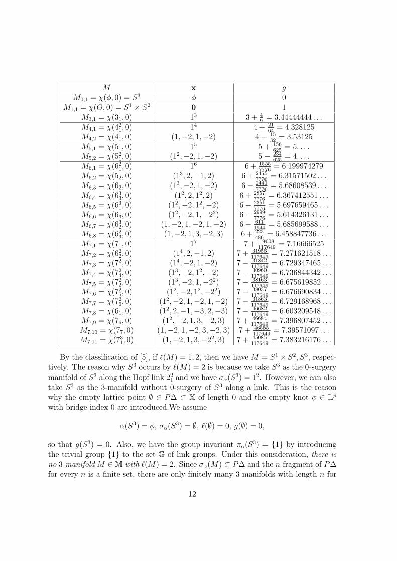
Table 4.1: The characteristic genera of 3-manifolds with lengths up to 7

11

M x gM0,1 = χ(ϕ, 0) = S3 ϕ 0

M1,1 = χ(O, 0) = S1 × S2 0 1M3,1 = χ(31, 0) 13 3 + 4

9= 3.44444444 . . .

M4,1 = χ(421, 0) 14 4 + 2164

= 4.328125M4,2 = χ(41, 0) (1,−2, 1,−2) 4− 15

32= 3.53125

M5,1 = χ(51, 0) 15 5 + 156625

= 5. . . .M5,2 = χ(521, 0) (12,−2, 1,−2) 5− 234

625= 4. . . .

M6,1 = χ(621, 0) 16 6 + 15557776

= 6.199974279M6,2 = χ(52, 0) (13, 2,−1, 2) 6 + 2455

7776= 6.31571502 . . .

M6,3 = χ(62, 0) (13,−2, 1,−2) 6− 24417776

= 5.68608539 . . .M6,4 = χ(633, 0) (12, 2, 12, 2) 6 + 2857

7776= 6.367412551 . . .

M6,5 = χ(631, 0) (12,−2, 12,−2) 6− 23517776

= 5.697659465 . . .M6,6 = χ(63, 0) (12,−2, 1,−22) 6− 2999

7776= 5.614326131 . . .

M6,7 = χ(632, 0) (1,−2, 1,−2, 1,−2) 6− 6111944

= 5.685699588 . . .M6,8 = χ(623, 0) (1,−2, 1, 3,−2, 3) 6 + 223

486= 6.458847736 . . .

M7,1 = χ(71, 0) 17 7 + 19608117649

= 7.16666525M7,2 = χ(622, 0) (14, 2,−1, 2) 7 + 31956

117649= 7.271621518 . . .

M7,3 = χ(721, 0) (14,−2, 1,−2) 7− 31842117649

= 6.729347465 . . .M7,4 = χ(724, 0) (13,−2, 12,−2) 7− 30960

117649= 6.736844342 . . .

M7,5 = χ(722, 0) (13,−2, 1,−22) 7− 38163117649

= 6.675619852 . . .M7,6 = χ(725, 0) (12,−2, 12,−22) 7− 38037

117649= 6.676690834 . . .

M7,7 = χ(726, 0) (12,−2, 1,−2, 1,−2) 7− 31863117649

= 6.729168968 . . .M7,8 = χ(61, 0) (12, 2,−1,−3, 2,−3) 7− 46682

117649= 6.603209548 . . .

M7,9 = χ(76, 0) (12,−2, 1, 3,−2, 3) 7 + 46684117649

= 7.396807452 . . .M7,10 = χ(77, 0) (1,−2, 1,−2, 3,−2, 3) 7 + 46555

117649= 7.39571097 . . .

M7,11 = χ(731, 0) (1,−2, 1, 3,−22, 3) 7 + 45085117649

= 7.383216176 . . .

By the classification of [5], if ℓ(M) = 1, 2, then we have M = S1 × S2, S3, respec-tively. The reason why S3 occurs by ℓ(M) = 2 is because we take S3 as the 0-surgerymanifold of S3 along the Hopf link 221 and we have σα(S

3) = 12. However, we can alsotake S3 as the 3-manifold without 0-surgery of S3 along a link. This is the reasonwhy the empty lattice point ∅ ∈ P∆ ⊂ X of length 0 and the empty knot ϕ ∈ Lp

with bridge index 0 are introduced.We assume

α(S3) = ϕ, σα(S3) = ∅, ℓ(∅) = 0, g(∅) = 0,

so that g(S3) = 0. Also, we have the group invariant πα(S3) = {1} by introducing

the trivial group {1} to the set G of link groups. Under this consideration, there isno 3-manifold M ∈ M with ℓ(M) = 2. Since σα(M) ⊂ P∆ and the n-fragment of P∆for every n is a finite set, there are only finitely many 3-manifolds with length n for

12

every n ≧ 0. According to the canonical well-order of X, the 3-manifolds of lengthn ≧ 1 are enumerated as follows:

Mn,1 < Mn,2 < · · · < Mn,mn

for a non-negative integer mn depending only on n. By the introduction of the emptyknot ϕ ∈ Lp, we put M0,1 = S3. By [5], we reconstruct from the lattice point σα(Mn,i)the link α(Mn,i) ∈ Lp, the group πα(Mn,i) ∈ G and the 3-manifold Mn,i itself. By(2) of Theorem 3.1, we reconstruct the lattice point σα(Mn,i) from the characteristicgenus g(Mn,i), so that we can construct from g(Mn,i) the lattice point σα(Mn,i), thelink α(Mn,i), the group πα(Mn,i) and the 3-manifold Mn,i itself.

In [KTB] the lattice points of the 3-manifolds Mn,i together with the geometricstructures for all n ≦ 10 are listed. In the following table, the characteristic generag(Mn,i) for all n ≦ 7 are given together with the data of the lattice point σα(Mn,i)and the link α(Mn,i) identified with a knot or a link in D. Rolfsen’s table [20], whereit is noted that there is no 3-manifold of length 2 by the reason stated above and atthis point the table is different from the tables of [5, 11, 12, 14].

For every 3-manifold M ∈ M with M = S3, S1 × S3, we have ℓ(M) ≧ 3. Every3-manifold M ∈ M has a Heegaard splitting, i.e., a union of two handlebodies bypasting along the boundaries. The Heegaard genus, gh(M) of M is the minimum ofthe genera of such handlebodies. The following lemma gives a relationship between abridge presentation of a link L ∈ L (see [3] for an explanation of bridge presentation)and Heegaard splittings of the Dehn surgery manifolds along L.

Lemma 4.2. Let a link L ∈ L have a g-bridge presentation. Then every Dehnsurgery manifold M of S3 along L admits a Heegaard splitting of genus g.

Proof. Since S3 is a union of two 3-balls B,B′ pasting along the boundary spheressuch that T = L ∩ B and T ′ = L ∩ B′ are trivial tangles of g proper arcs in B andB′, respectively. Let N(T ) be a tubular neighborhood of T in B, V = cl(B \N(T )),and V ′ = B′ ∪ N(T ). By construction, V and V ′ are handlebodies of genus g andforms a Heegaard splitting of S3. To complete the proof, it suffices to show that theDehn surgery from S3 to M along L just changes V ′ into another handlebody V ′′,so that V and V ′′ forms a Heegaard splitting of M of genus g. Since T ′ is a trivialtangle in B′ of g proper arcs, there are g − 1 proper disks Di (i = 1, 2, . . . , g − 1) inB′ which split B′ into a 3-manifold regarded as a tubular neighborhood N(T ′) of T ′

in B′. Then the union N(L) = N(T ) ∪N(T ′) is regarded as a tubular neighborhoodof L in S3. The Dehn surgery from S3 to M along L just changes N(L) into theunion of solid tori obtained from N(L) by the Dehn surgery without changing theboundary ∂N(L). Thus, we obtain the desired handlebody V ′′ by pasting along thedisks corresponding to Di (i = 1, 2, . . . , g − 1).

13

Let gb(M) and gbr(M) denote respectively the bridge genus and the braid genusof M , namely the minimal bridge index and the minimal braid index for links whose0-surgery manifolds are M . We define gb(S

3) = gbr(S3) = 0 by considering that S3 is

obtained from S3 by the 0-surgery along the empty knot ϕ. The 3-manifold M withℓ(M) ≧ 3 is ending-positive or ending-negative, respectively, according to whetherσα(M) is ending-positive or ending-negative. Then we have the following lemma:

Lemma 4.3. For every M ∈ M with ℓ(M) ≧ 3, we have

2gh(M)− 2 ≦ 2gb(M)− 2 ≦ 2gbr(M)− 2 ≦ ℓ(M) < g(M) + end(M),

where end(M) is 0 or 12, respectively, according to whether M is ending-positive or

ending-negative.

Proof. By Lemmas 2.3 and 4.2, we have

gh(M) ≦ gb(M) ≦ gbr(M) ≦ ℓ(M)

2+ 1.

By Theorem 3.1 (1), according to whether M is ending-positive or ending-negative,the inequality ℓ(M) < g(M) or ℓ(M) < g(M) + 1

2holds, respectively, from which the

result follows.

We show the following theorem:

Theorem 4.4. The characteristic genus g(M) of every M ∈ M is a characteristicinvariant defined for M such that

gh(S3) = gb(S

3) = gbr(S3) = g(S3) = ℓ(S3) = 0,

gh(S1 × S3) = gb(S

1 × S3) = gbr(S1 × S3) = g(S1 × S3) = ℓ(S1 × S3) = 1

and every M ∈ M withM = S3, S1 × S3 has the following properties:

(1) The 3-manifold M itself, the lattice point σα(M), the link α(M) and the groupπα(M) are reconstructed from the value of g(M).

(2) According to whether M is ending-positive or ending-negative, the characteristicgenus g(M) belongs to (n, n+ 1

2)Q or (n− 1

2, n)Q for n = ℓ(M).

(3) There are only finitely many 3-manifolds M ∈ M such that

g(M) ∈ (n− 1

2, n+

1

2)Q.

14

(4) The inequalities

2gh(M)− 2 ≦ 2gb(M)− 2 ≦ 2gbr(M)− 2 ≦ ℓ(M) < g(M) + end(M)

hold, where end(M) is 0 or 12, respectively, according to whether M is ending-positive

or ending-negative.

Proof. By definition, we have the values of S3 and S1×S2.By the property of σα in[5] and Theorem 3.1, it is seen that g(M) is a characteristic rational invariant definedfor M and the properties (1)-(3) hold. (4) is obtained in Lemma 4.3.

The following corollary is direct from Theorem 4.5 (3).

Corollary 4.5. For any infinite subset M′ ⊂ M, we have

sup{ℓ(M)|M ∈ M′} = +∞.

For every integer n > 1, since there are infinitely many 3-manifolds M ∈ M withgbr(M) ≦ n, we see from Corollary 4.5 that there are lots of 3-manifolds M ∈ M suchthat the difference ℓ(M)− gbr(M) is sufficiently large. However, exact calculations ofthe invariants gb(M), gbr(M), ℓ(M) for most 3-manifolds are not known and remainas an open problem. Here are some elementary examples.

Example 4.6. (1) Let M = χ(31, 0) = M3,1 for the trefoil knot 31. Since the braidindex of 31 is 2 and M is not the lens space, we see from Table 4.1 that

gh(M) = gb(M) = gbr(M) = 2 <ℓ(M)

2+ 1 = 2.5 and g(M) = 3 +

4

9= 3.444 . . . .

(2) Let M = χ(421, 0) = M4,1 for the (2, 4)-torus link 421. Since the braid index of421 is 2 and the first integral homology H1(M) has exactly 2 generators, we see fromTable 4.1 that

gh(M) = gb(M) = gbr(M) = 2 <ℓ(M)

2+ 1 = 3 and g(M) = 4 +

21

64= 4.328 . . . .

(3) Let M = χ(41, 0) = M4,2 for the figure eight knot 41. Since the bridge indexof 41 is 2 and M is not any lens space, we see that gh(M) = gb(M) = 2. If M isobtained from a knot or link of braid index 2, then M would be obtained from a(2k + 1)-half-twist knot K(k) by 0-surgery. However, this is impossible because theAlexander polynomial of the homology handles M and M(k) = χ(K(k), 0) are

AM(t) = t2 − 3t+ 1, AM(k) =t2k+1 + 1

t+ 1

15

and they are distinct. These results and Table 4.1 mean that

gh(M) = gb(M) = 2 < gbr(M) =ℓ(M)

2+ 1 = 3 < g(M) = 4− 15

32= 3.531 . . . .

We note here that the bridge genus behaves differently from the Heegaard genus,although gh(M) = gb(M) in Example 4.6. For example, if M is a lens space except S3

and S1×S2, then we have gb(M) ≧ 3 whereas gh(M) = 1. In fact, the first homologyH1(M) is a non-trivial finite cyclic group. Onthe other hand, if 1 ≦ gb(M) ≦ 2,then H1(M) would be isomorphic to the infinite cyclic group Z or a direct doubleZ/mZ⊕Z/mZ for some m ≧ 0, which is a contradiction. Concretly, the pro—ective3-space M = P 3 has σα(M) = (12, 2, 12, 2) (see [5, 14]) and hence gb(M) = 3. Bydeveloping a similar consideration, S. Okazaki[19] has observed a linear independenceon the Heegaard genus gh(M), the bridge genus gb(M) and the braid genus gbr(M).

5. Constructing a characteristic smooth real function defined for thePDelta set

A PDelta subset is a subset S of the PDelta set P∆ containing the lattice points∅ and 0.3 Let a and t be real numbers such that either −1 ≦ a ≦ 1 and −1 < t < 1or −1 < a < 1 and −1 ≦ t ≦ 1. Then the linear fraction

B(t; a) =t− a

1− at

is considered. If |t| < 1 and |a| < 1, then |B(t; a)| < 1, because we have

1− |B(t; a)|2 = (1− t2)(1− a2)

(1− at)2.

If |a| = 1 or |t| = 1, then it is easily checked that |B(t; a)| = 1. In fact, we haveB(t;±1) = B(∓1, a) = ∓1.

Noting that the decimal torsions of ∅, 0 and 12 are not definite values as it isexplained in Remark 3.2, we put the following definition for any x ∈ P∆:

Gx(t) =

B(t; τ(x)) (ℓ(x) ≧ 3)B(t; 1) = −1 (x = 12)B(t;−1) = 1 (x = ∅, 0)

For every n-fragment S(n) of a PDelta subset S ⊂ P∆, the function

G(n)S (t) =

∏x∈S(n)

Gx(t)

3This condition is imposed for simplicity.

16

is called a finite Blaschke product4 whose zero’s are precisely the decimal torsions τ(x)for all x ∈ S(n) except ∅,0 and 12. By the assumption of the set S, we have

G(0)S (t) = G

(1)S (t) = 1.

Further, according to whether the lattice point 12 belongs to S or not, we haveG

(2)S (t) = −1 or 1, respectively. For example, when we take S = Lp, the functions

G(n)Lp (t) for n = 0, 1, 2, 3, 4, 5 are calculated as follows:

G(0)Lp (t) = 1,

G(1)Lp (t) = 1,

G(2)Lp (t) = −1,

G(3)Lp (t) = −G13(t) = −B(t;

4

9),

G(4)Lp (t) = −G13(t)Q14(t)G(1,−2,1,−2)(t) = −B(t;

4

9)B(t;

21

64)B(t;

−15

32),

G(5)Lp (t) = −G13(t)G14(t)G(1,−2,1,−2)(t)G15(t)G(12,−2,1,−2)(t)

= −B(t;4

9)B(t;

21

64)B(t;

−15

32)B(t;

156

625)B(t;

−234

625).

We obtain the following theorem.

Theorem 5.1. For every PDelta subset S, the series function

GS(t) =+∞∑n=0

G(n)S (t)tn

is a smooth real function defined on the interval (−1, 1) which is a characteristicinvariant defined for the set S.

Proof. Since |G(n)S (t)| ≦ 1 for any n, we have

|GS(t)| ≦+∞∑n=0

|t|n =1

1− |t|.

This means that the series GS(t) defined on (−1, 1) is uniformly convergent in the

wide sense. Using that the function G(n)S (t) (t ∈ (−1, 1)) is uniformly convergent

in the wide sense, we see from the Weierstrass double series theorem that the series

4See Blaschke [2]. The author thanks to K. Sakan for suggesting the Blaschke product.

17

function GS(t) is a smooth real function defined on (−1, 1). To see that the functionGS(t) is characteristic for S, it suffices to see by induction on n ≧ 2 that the set of thedecimal torsions τ(x) for all lattice points x ∈ S(n) except ∅, 0 is determined by thefunction GS(t). According to whether 12 is in S or not, the second derivative d2

dt2GS(0)

is −2 or 2, respectively. Thus, S(2) is determined by the function GS(t). Assume thatall the lattice points of S(n−1) (n− 1 ≧ 2) are determined by the function GS(t). Let

G(n)S (t) = GS(t)−

n−1∑i=0

G(i)S (t)ti.

The function G(n)S (t) has the following splitting form:

G(n)S (t) = G

(n)S (t) · G(t) · tn,

where

G(t) = 1 + G(n+1)S (t)t+ G

(n+2)S (t)t2 + G

(n+3)S (t)t3 + . . .

for some finite Blaschke products G(n+i)S (t) with

G(n)S (t) · G(n+i)

S (t) = G(n+i)S (t)

for all i (i = 1, 2, 3, . . . ). We show that the function G(t) has no zero’s in the interval(−1

2, 12). In fact, we have

|G(t)| ≧ 1−+∞∑i=1

|t|i = 1− 2|t|1− |t|

> 0

for any t with |t| < 12. This means that the decimal torsions τ(x) for all lattice points

x ∈ S(n) except ∅, 0 and 12 are characterized by the zero’s of the function G(n)S (t) in

the interval (−12, 12) \ {0}.

It is noted that the series function GS(t) does not converge for t = ±1. This isbecause

limn→+∞

|G(n)S (±1) · (±1)n| = 1 = 0.

The function GS(t) is called the characteristic genus function defined for the PDeltasubset S. For example, for S = {∅,0}, we have

GS(t) = 1 + t+ t2 + t3 + · · · = 1

1− t.

18

For S = {∅,0, 12}, we have

GS(t) = 1 + t− (t2 + t3 + t4 + . . . ) = 1 + t− t2

1− t.

For a finite set S with the maximal length n,

GS(t) =n−1∑i=0

G(i)S (t)ti +G

(n)S (t)

tn

1− t.

For the subset S = σ(Lp), we denote G(n)S (t) and GS(t) by G

(n)Lp (t) and GLp(t),

respectively. The following corollary is direct from Theorem 5.1.

Corollary 5.2. The series function

GLp(t) =+∞∑n=0

G(n)Lp (t)tn

= 1 + t− t2 −B(t,4

9)t3 −B(t,

4

9)B(t,

21

64)B(t,

−15

32)t4

−B(t,4

9)B(t,

21

64)B(t,

−15

32)B(t,

156

625)B(t,

−234

625)t5 + . . .

is a smooth real function defined on the interval (-1, 1) which is a characteristicinvariant defined for the prime link set Lp.

For example, let L(2, ∗) be the set of (2, n)-torus links regarding the (2, 0)-toruslink as the empty knot ϕ. Since

σ(L(2, ∗)) = {1n|n = 0, 1, 2, 3, . . . },

where 10 = ϕ, 1 = 0 and τ(1n) = 1n−1

− 1nn−nn−1 for n ≧ 3, we have:

GL(2,∗)(t) = 1 + t− t2 −+∞∑n=3

(n∏

k=3

B

(t,

1

k − 1− 1

kk − kk−1

))tn.

For the subset S = σα(M), we denote G(n)S (t) and GS(t) by G

(n)M (t) and GM(t),

respectively. Noting that the lattice point 12 is excluded from σ(M) (by the reasonthat the empty lattice point ∅ is introduced), we have the following corollary obtainedfrom Theorem 5.1.

19

Corollary 5.3 The series function

GM(t) =+∞∑n=0

G(n)M (t)tn

= 1 + t+ t2 +B(t;4

9)t3 +B(t;

4

9)B(t;

21

64)B(t;

−15

32)t4

+B(t;4

9)B(t;

21

64)B(t;

−15

32)B(t;

156

625)B(t,

−234

625)t5 + . . . .

is a smooth real function defined on the interval (−1, 1) which is a characteristicinvariant defined for the 3-manifold set M.

Acknowledgements. This work was supported by JSPS KAKENHI Grant Number24244005.

References

[1] J. S. Birman, Braids, links, and mapping class groups, Ann. Math. Studies, 82(1974), Princeton Univ. Press.

[2] W. Blaschke, Eine Erweiterung des Satzes von Vitali uber Folgen analytis-cher Funktionen, Berichte Math.-Phys. Kl., Sachs. Gesell. der Wiss. Leipzig,67 (1915), 194-200.

[3] A. Kawauchi, A survey of knot theory, (1996), Birkhauser.

[4] A. Kawauchi, Topological imitation of a colored link with the same Dehn surgerymanifold, in: Proceedings of Topology in Matsue 2002, Topology Appl., 146-147(2005), 67-82.

[5] A. Kawauchi, A tabulation of 3-manifolds via Dehn surgery, Boletin de la So-ciedad Matematica Mexicana (3), 10 (2004), 279-304.

[6] A. Kawauchi and I. Tayama, Enumerating the prime knots and links bya canonical order, in: Proc. 1st East Asian School of Knots, Links, andRelated Topics (Seoul, Jan. 2004), (2004), 307-316. (http://www.sci.osaka-cu.ac.jp/˜kawauchi/index.htm)

[7] A. Kawauchi and I. Tayama, Enumerating the exteriors of prime links by acanonical order, in: Proc. Second East Asian School of Knots, Links, andRelated Topics in Geometric Topology (Darlian, Aug. 2005), (2005), 269-277.(http://www.sci.osaka-cu.ac.jp/˜kawauchi/index.htm)

20

[8] A. Kawauchi and I. Tayama, Enumerating prime links by a canonical order,Journal of Knot Theory and Its Ramifications, 15 (2006), 217-237.

[9] A. Kawauchi and I. Tayama, Enumerating 3-manifolds by a canonical order,Intelligence of low dimensional topology 2006, Series on Knots and Everything,40 (2007), 165-172.

[10] A. Kawauchi and I. Tayama, Enumerating prime link exteriors with lengths upto 10 by a canonical order, Proceedings of the joint conference of Intelligence ofLow Dimensional Topology 2008 and the Extended KOOK Seminar (Osaka, Oct.2008), (2008), 135-143. (http://www.sci.osaka-cu.ac.jp/ kawauchi/index.htm)

[11] A. Kawauchi and I. Tayama, Enumerating homology spheres with lengths up to10 by a canonical order, Proceedings of Intelligence of Low-Dimensional Topology2009 in honor of Professor Kunio Murasugi’s 80th birthday (Osaka, Nov. 2009),(2009), 83-92. (http://www.sci.osaka-cu.ac.jp/ kawauchi/index.htm)

[12] A. Kawauchi and I. Tayama, Enumerating 3-manifolds with lengths up to 9 bya canonical order, Topology Appl., 157 (2010), 261-268.

[13] A. Kawauchi and I. Tayama, Representing 3-manifolds in the complex numberplane, preprint. (http://www.sci.osaka-cu.ac.jp/˜kawauchi/index.htm)

[14] A. Kawauchi, I. Tayama and B. Burton, Tabulation of 3-manifolds of lengthsup to 10, Proceedings of International Conference on Topology and Geometry2013, joint with the 6th Japan-Mexico Topology Symposium, Topology and itsApplications (to appear). http://dx.doi.org/10.1016/j.topol.2015.05.036

[15] B. von Kerekjarto, Vorlesungen uber Topologie, Spinger, Berlin, 1923.

[16] R. Kirby, A calculus for framed links in S3, Invent. Math., 45(1978), 35-56.

[17] J. Milnor and W. Thurston, Characteristic numbers of 3-manifolds, EnseignmentMath., 23(1977), 249-254.

[18] Y. Nakagawa, A family of integer-valued complete invariants of oriented knottypes, J. Knot Theory Ramifications, 10(2001), 1160-1199.

[19] S. Okazaki, On Heegaard genus, bridge genus and braid genus for a3-manifold, J. Knot Theory Ramifications, 20 (2011), 1217-1227. DOI:10.1142/S0218216511009145

[20] D. Rolfsen, Knots and links, (1976), Publish or Perish.

21