characterisation and modelling of...

CHARACTERISATION AND MODELLING OF STATIC RECOVERY PROCESS OF ALUMINUM ALLOY

MOHD AZIZI BIN JUNIT

UNIVERSITI MALAYSIA PAHANG

CHARACTERISATION AND MODELLING OF STATIC RECOVERY PROCESS OF ALUMINUM ALLOY

MOHD AZIZI BIN JUNIT

A report submitted in partial fulfillmentof the requirements for the award of the degree of

Bachelor of Mechanical Engineering

Faculty of Mechanical EngineeringUNIVERSITI MALAYSIA PAHANG

NOVEMBER 2008

vii

ABSTRACT

A comprehensive study of the annealing behavior of aluminum alloy has been

carried out in this research. The primary objectives of this work have been to study

the effect of recovery on the annealing behavior and to validate the static recovery

process of aluminum alloy using Friedel’s model. Annealing is a heat treatment

process used to eliminate the residual stresses produced during cold work and static

recovery is one of the processes in annealing. This process is the most subtle stage of

annealing and no gross microstructure change occurred. In this research, aluminum

alloy were to undergo thermo-mechanical process which compression test and

annealing process took place. The experimental part has focused on characterisation

of the softening reaction. Through this test, the material was tested at different pre-

strain which is 2.5%,5%.7.5% and 10% to see the difference stress due to recovery

temperature(100oC,150oC,200oC,250oC) and time(1hour,2hour,3hour,4hour). Then,

the graph for relationship between degree of recovery,Xrec with temperature, time

and pre-strain are plotted. Friedel’s model equation is applied to the experimental

result to find the activation energy,Q. For the relationship between degree of

recovery,Xrec and temperature, the activation energy,Q is about 732.55 kJ/mol while

the activation energy,Q for relationship between degree of recovery,Xrec and time is

224.83 kJ/mol. Finally, the activation energy,Q value from the experimental result

are compared with literature review to validate the static recovery process of

aluminum alloy using Friedel’s model equation.

viii

ABSTRAK

Pembelajaran menyeluruh tentang sifat sepuh lindap untuk aloi aluminium telah

dilaksanakan di dalam kajian ini. Objektif utama kajian ini ialah mempelajari kesan

pemulihan ke atas sifat sepuh lindap dan untuk mengesahkan proses pemulihan statik

untuk aloi aluminium dengan menggunakan model Friedel. Sepuh lindap ialah

pemulihan haba untuk menyingkirkan sisa tekanan yang terhasil dari kerja sejuk dan

pemulihan statik ialah salah satu proses sepuh lindap. Proses ini merupakan

peringkat yang paling halus di dalam sepuh lindap dan tiada perubahan struktur

mikro yang kasar akan berlaku. Di dalam kajian ini, aloi aluminium akan melalui

proses thermo-mekanikal iaitu ujian tekanan dan proses sepuh lindap. Bahagian

eksperimental hanya tertumpu kepada ciri-ciri tindak balas kelembutan. Melalui

ujian ini, bahan akan diuji dengan pra-ketegangan yang berbeza iaitu 2.5%,5%,7.5%

dan 10% untuk melihat perbezaan tekanan dari segi pemulihan

suhu(100oC,150oC,200oC,250oC) dan masa(1jam,2jam,3jam,4jam). Selepas itu, graf

untuk hubungan darjah pemulihan,X dengan suhu,masa dan pra-ketegangan

dihubung kaitkan. Persamaan model Friedel digunakan ke atas hasil eksperimental

untuk mendapatkan tenaga pengaktifan,Q. Untuk hubungan di antara darjah

pemulihan,X dan suhu, nilai tenaga pengaktifan,Q ialah 732.55 kJ/mol manakala

nilai tenaga pengaktifan,Q untuk hubungan antara darjah pemulihan,X dan masa

ialah 224.83 kJ/mol. Akhirnya, nilai untuk tenaga pengaktifan,Q yang dikira

daripada eksperimental akan dibandingkan dengan rujukan untuk mengesahkan

proses pemulihan statik untuk aloi aluminium dengan menggunakan persamaan

model Friedel.

ix

TABLE OF CONTENTS

Page

SUPERVISOR’S DECLARATION iii

STUDENT’S DECLARATION iv

ACKNOWLEDGEMENTS vi

ABSTRACT vii

ABSTRAK viii

TABLE OF CONTENTS ix

LIST OF TABLES xii

LIST OF FIGURES xiii

LIST OF SYMBOLS xiv

LIST OF ABBREVIATIONS xv

CHAPTER 1 INTRODUCTION

1.1 Background 1

1.2 Problem Statements 2

1.3 Objectives 2

1.4 Scope of Project 2

1.5 Methodology 2

CHAPTER 2 LITERATURE REVIEW

2.1 Annealing 4

2.1.1 Recovery 5 2.1.2 Recrystallization 6 2.1.3 Grain Growth 6

2.2 Compression Test 7

2.3 Engineering Stress and Strain 7

2.3.1 Engineering Stress 7

x

2.3.2 Engineering Strain 7

2.4 Properties Obtained from Compression Test 8

2.4.1 Yield Strength 82.4.2 Ultimate Tensile Strength 92.4.3 Percent Elongation 92.4.4 Modulus of Elasticity 102.4.5 Percent Reduction in Area 10

2.5 Material 10

2.6 Friedel’s Model 11

2.7 Reverse Calculation from Published Result 12

CHAPTER 3 METHODOLOGY

3.1 Introduction 15

3.2 Machining Process 15

3.2.1 Bandsaw 153.2.2 Lathe Machine 16

3.2.2.1 Three important element 173.2.2.2 Precaution Steps 18

3.3 Annealing Process 19

3.3.1 Precaution Steps 19

3.4 Pre-Strain the Specimens 20

3.5 Recovery Process 20

3.6 Pre-Strain Recovered Specimens 21

3.7 Analyzing Data 21

3.8 Applying Friedel’s Model 22

3.9 Comparison 22

CHAPTER 4 RESULT AND DISCUSSIONS

4.1 Introduction 23

4.2 Result 23

4.2.1 Relationship between Xrec versus 1/T 244.2.1.1 Calculation from Graph 26

4.2.2 Relationship between Xrec versus ln t 274.2.2.1 Calculation from Graph 29

xi

4.2.3 Relationship between Xrec versus Pre-strain 304.2.3.1 Calculation from Graph 32

4.3 Discussion 33

4.3.1 Specimen Error 334.3.2 Time 344.3.3 Temperature 344.3.4 Environmental Aspect 34

4.4 Comparison 35

CHAPTER 5 CONCLUSION AND RECOMMENDATIONS

5.1 Summary 37

5.2 Conclusions 38

5.3 Recommendations 39

REFERENCES 40

APPENDICES A 41

APPENDICES B 43

xii

LIST OF TABLES

Table No. Page

2.1 Mechanical and physical properties of Aluminum alloy AA1100 10

4.1 Data for temperature 100oC at 5% and 1 hour 24




4.5 Data for time 1 hour at 5% and 150oC 27




4.9 Data for pre-strain 2.5% at 150oC and 1 hour 30

4.10 Data for pre-strain 5% at 150oC and 1 hour 30

4.11 Data for pre-strain 7.5% at 150oC and 1 hour 30

4.12 Data for pre-strain 10% at 150oC and 1 hour 31

4.13 Activation energy for graph Xrec vs ln t 35

4.14 Activation energy for graph Xrec vs 1/T 36

xiii

LIST OF FIGURES

Figure No. Page

1.1 Flowchart of research methodology 3

2.1 Effect of annealing on the structure and mechanical property changes 5

2.2 Example of recovery microstructure 6

2.3 Engineering stress-strain diagram 8

2.4 Determination of reloading flow stress and degree of softening by the back extrapolation(be) and offset(os) 12

2.5 Graph Xrec versus time with different temperature 12

2.6 Graph Xrec versus 1/T 13

3.1 Mechanical bandsaw 16

3.2 Mechanical lathe machine 16

3.3 Lathe machine process 17

3.4 Box furnace 19

3.5 Compression test 20

4.1 Graph Xrec versus 1/Temperature 25

4.2 Graph Xrec versus ln time 28

4.3 Graph Xrec versus pre-strain 31

4.4 Error resulting from machining 33

xiv

LIST OF SYMBOLS

Xrec Degree of recovery

σm Yield stress of the as deformed crystal

σr Yield stress of the recovered crystal

σo Yield stress of undeformed crystal

Q Activation energy

R Gas constant

T Temperature

t Time

C1 Constant

xv

LIST OF ABBREVIATIONS

Al Aluminum

be Back extrapolation

os Offset

CNC Computer numerical control

rpm Revolution per minute

CHAPTER 1

INTRODUCTION

Annealing is one of the most important processes in industry. The term

annealing refers to a heat treatment in which a material is exposed to an elevated

temperature for an extended time period and then slowly cooled. Annealing is a heat

treatment used to eliminate some or all of the effects of cold working. Ordinarily,

annealing is carried out to relieve stresses and produce a specific microstructure. It

also used to increase softness, ductility and toughness of metal.

Static recovery is one of the processes in annealing. The recovery

temperature is heated just below the recrystallization temperature range. This process

is the most subtle stage of annealing and no gross microstructure change occurs.

During recovery, sufficient thermal energy is supplied to allow the dislocations to

rearrange themselves into lower energy configurations. Recovery of many cold

worked metals produces a subgrain structure with low angle grain boundaries and is

this recovery process called polygonization. During recovery, the strength of a cold

worked metal is reduced only slightly but its ductility is usually increased.

1.1 BACKGROUND

Aluminum alloys have found wide acceptance in engineering design

primarily because they are relative lightweight and have a high strength to weight

ratio. They also have a superior corrosion resistance and comparatively inexpensive.

For some applications they are favored because of their high thermal and electrical

conductivity, ease of fabrication and ready availability. Generally, the strengths of

aluminum alloys decrease and toughness increases with increase in temperature and

2

with time at temperature above room temperature. Aluminum is easily fabricated. It

can be cast by any method like rolled to any reasonable thickness, stamped,

hammered, forged or extruded. It also readily turned, milled, bored or machined.

Pure aluminum has low compression strength but when combined with thermo-

mechanical processing aluminum alloy display a marked improvement in mechanical

properties. The main application of aluminum is used in aircraft and rockets.

1.2 PROBLEM STATEMENTS

The problem statements are:

(a) We want to find the different of stress before and after static recovery

process.

(b) Investigation of static recovery process due to influenced of pre strain,

temperature and time.

1.3 OBJECTIVES

The research objective is to validate the static recovery process of aluminum alloy

using Friedel’s Model.

1.4 SCOPES OF PROJECT

(a) In this research, the material used is limited to aluminum alloy only.

(b) Test the specimen using compression test.

(c) Varying pre-strain about 2.5%, 5%, 7.5% and 10%.

(d) Perform the annealing using the box furnace.

1.5 METHODOLOGY

This research is conducted under several main steps. The major steps for this

research are the material will go the compression test under a several pre-strain.

Then, perform the annealing process to specimens using the box furnace. After that,

3

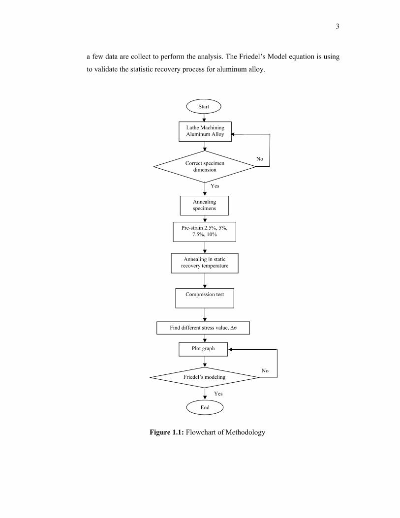
a few data are collect to perform the analysis. The Friedel’s Model equation is using

to validate the statistic recovery process for aluminum alloy.

Figure 1.1: Flowchart of Methodology

Lathe Machining Aluminum Alloy

Correct specimen dimension

Annealing specimens

Compression test

Find different stress value, ∆σ

Friedel’s modeling

Annealing in static recovery temperature

Plot graph

No

Pre-strain 2.5%, 5%, 7.5%, 10%

Start

Yes

End

Yes

No

CHAPTER 2

LITERATURE REVIEW

The literature review and background knowledge of static recovery process

and how it related with Friedel’s Model are presented in this chapter.

2.1 ANNEALING

Annealing is a heat treatment used to eliminate some or all of the effects of

cold working. Annealing at low temperature maybe used to eliminate the residual

stresses produced during cold working without affecting the mechanical properties of

the finish part. Annealing also may be used to complete eliminate the strain

hardening achieved during cold working. In this case, the final part is soft and ductile

but still has a good surface finish and dimensional accuracy. After annealing,

additional cold work could be done, since the ductility is restored by combining

repeated cycles of cold working and annealing, large total deformations maybe

achieved.

There are three stages in the annealing process, with the first being the

recovery phase, which results in softening of the metal through removal of crystal

defects (the primary type of which is the linear defect called a dislocation) and the

internal stresses which they cause. The second phase is recrystallization, where new

grains nucleate and grow to replace those deformed by internal stresses. If annealing

is allowed to continue once recrystallization has been completed, grain growth will

occur, in which the microstructure starts to coarsen and may cause the metal to have

less than satisfactory mechanical properties. [1]

5

Figure 2.1: Effect of annealing on the structure and mechanical property changes.[3]

2.1.1 Recovery

Recovery is one of the process in annealing.The original cold-worked

microstructure is composed of deformed grains containing a large number of tangled

dislocations. When we first heat the metal, the additional thermal energy permits the

dislocations to move and form the boundaries of a polygonized sub grain structure.

The dislocation density however is virtually unchanged. This low temperature

treatment removes the residual stresses due to cold working without causing a

change in dislocation density and is called recovery. The mechanical properties of

the metal are relatively unchanged because the number of dislocations is not reduced

during recovery. However, since residual stresses are reduced or even eliminated

when the dislocations are rearranged and is often called a stress relief anneals. [1]

6

Figure 2.2: Example of recovery microstructure. [5]

2.1.2 Recrystallization

When a cold worked metallic material is heated above a certain temperature,

rapid recovery eliminates residual stresses and produced a polygonized dislocation

structure. New small grains then nucleate at the cell boundaries of the polygonized

structure, eliminating most of the dislocations. Because the number of dislocations is

greatly reduced, the recrystallized metal has low strength but high ductility. The

temperature at which a microstructure of new grains that have very low dislocation

density appears is known as the recrystallization temperature. The process of

formation of new grains by heat treating a cold worked material is known as

recrystallization. [1]

2.1.3 Grain Growth

At still higher annealing temperatures, both recovery and recrystallization

occur rapidly, producing a fine recrystallized grain structure. If the temperature is

high enough, the grains begins to grow with favored grains consuming the smaller

grains. This phenomenon called grain growth is driven by the reduction in grain

boundary area. [1]

7

2.2 COMPRESSION TEST

The compression test is a method for determining behavior of materials under

crushing loads. Specimen is compressed and deformation at various loaded is

recorded. Compressive stress and strain are calculated and plotted as a stress-strain

diagram which is used to determine elastic limit, proportional limit, yield point, yield

strength and compressive strength. [3]

2.3 ENGINEERING STRESS AND STRAIN

The results of a compression test apply to all sizes and cross-sections of

specimens for given material if we convert the force to stress and the distance

between gage marks to strain.

2.3.1 Engineering Stress

oA

F

Where;

F = instantaneous load applied perpendicularly to the specimen cross section.

Ao = the original cross sectional area before any load is applied

2.3.2 Engineering Strain

ε =o

oi

l

ll )(

Where;

l o = original length before any load applied

l i = the instantaneous length

8

Figure 2.3: Engineering stress-strain diagram. [1]

2.4 PROPERTIES OBTAINED FROM COMPRESSION TEST

2.4.1 Yield Strength

As we apply stress to a material, the material initially exhibits elastic

deformation. The strain that develops is completely recovered when the applied

stress is removed. However, as we continue to increase the applied stress the

materials begins to exhibit both elastic and plastic deformation. The material

eventually yields to the applied stress. The critical stress value needed to initiate

plastic deformation is defined as the elastic limit of the material. The proportional

limit is defined as the level of the stress above which the relationship between stress

and strain is not linear. [1]

In most materials the elastic limit and proportional limit are quite close.

However, neither the elastic limit nor the proportional limit values can be determined

precisely. Measured values depend on the sensitivity of the equipment used and

defined as offset strain value (typically is 0.2%). Then, draw a line starting with this

offset value of strain and draw a line parallel to the linear portion of the engineering

stress-strain curve. The stress value corresponding to the intersection of this line and

9

the engineering stress-strain curve is defined as the offset yield strength, also often

stated as yield strength.

2.4.2 Ultimate Tensile Strength

The ultimate tensile strength is the maximum strength reached in the

engineering stress-strain curve. If the specimen develops a localized decrease in

cross-sectional area (commonly called necking), the engineering stress will decrease

with further strain until fracture occurs since the engineering stress is determined by

using the original cross-sectional area of the specimen. The more ductile a metal is,

the more the specimen will neck before fracture and hence the more the decrease in

the stress on the stress-strain curve beyond the maximum stress.

The ultimate tensile strength of a metal is determined by drawing a horizontal

line from the maximum point on the stress-strain curve to the stress axis. The stress

where this line intersects the stress axis is called the ultimate tensile strength or

sometimes just the tensile strength. The ultimate tensile strength is not used much in

engineering design for ductile alloys since too much plastic deformation takes place

before it is reached. However, the ultimate tensile strength can give some indication

of the presence of defects. If the metal contains porosity or inclusions, these defects

may cause the ultimate tensile strength of the metal to be lower than normal. [3]

2.4.3 Percent Elongation

The amount of elongation that a tensile specimen undergoes during testing

provides a value for the ductility of the metal. Ductility of the metals is most

commonly expressed as percent elongation, starting with a gage length usually of

5.1cm. In general, the higher the ductility (the more deformable the metal is), the

higher the percent elongation is.

The percent elongation at fracture is of the engineering importance not only

as a measure of ductility but also as an index of the quality of the metal. If porosity

or inclusions are present in the metal or if damage due to overheating the metal has

10

occurred, the percent elongation of the specimen tested may be decreased below

normal. [3]

2.4.4 Modulus of Elasticity

In the first part of tensile test, the material is deformed elastically. That is, if

the load on the specimen is released, the specimen will return to its original length.

For metals the maximum elastic deformation is usually less than 0.5 percent. The

modulus of elasticity is related to the bonding strength between the atoms in metal

and alloy. Metals with high elastic modules are relatively stiff and do not deflect

easily. In the elastic region of the stress-strain diagram, the modulus does not change

with increasing stress. [3]

2.4.5 Percent Reduction in Area

The ductility of a metal or alloy can also be expressed in terms of the percent

reduction in area. The percent reduction in area, like the percent elongation, is

measure of the ductility of the metal and is also an index of quality. The percent

reduction in area may be decreased if defects such as inclusions or porosity are

present in the metal specimen. [3]

2.5 MATERIAL

Table 2.1: Mechanical and physical properties of Aluminum alloy AA1100.

Properties Value

Yield strength 103MPa

Ultimate strength 110MPa

Elongation at break 12%

Modulus of elasticity 69GPa

Melting point 540.6oC – 643oC

Annealing temperature 413oC

Recovery temperature 150oC

11

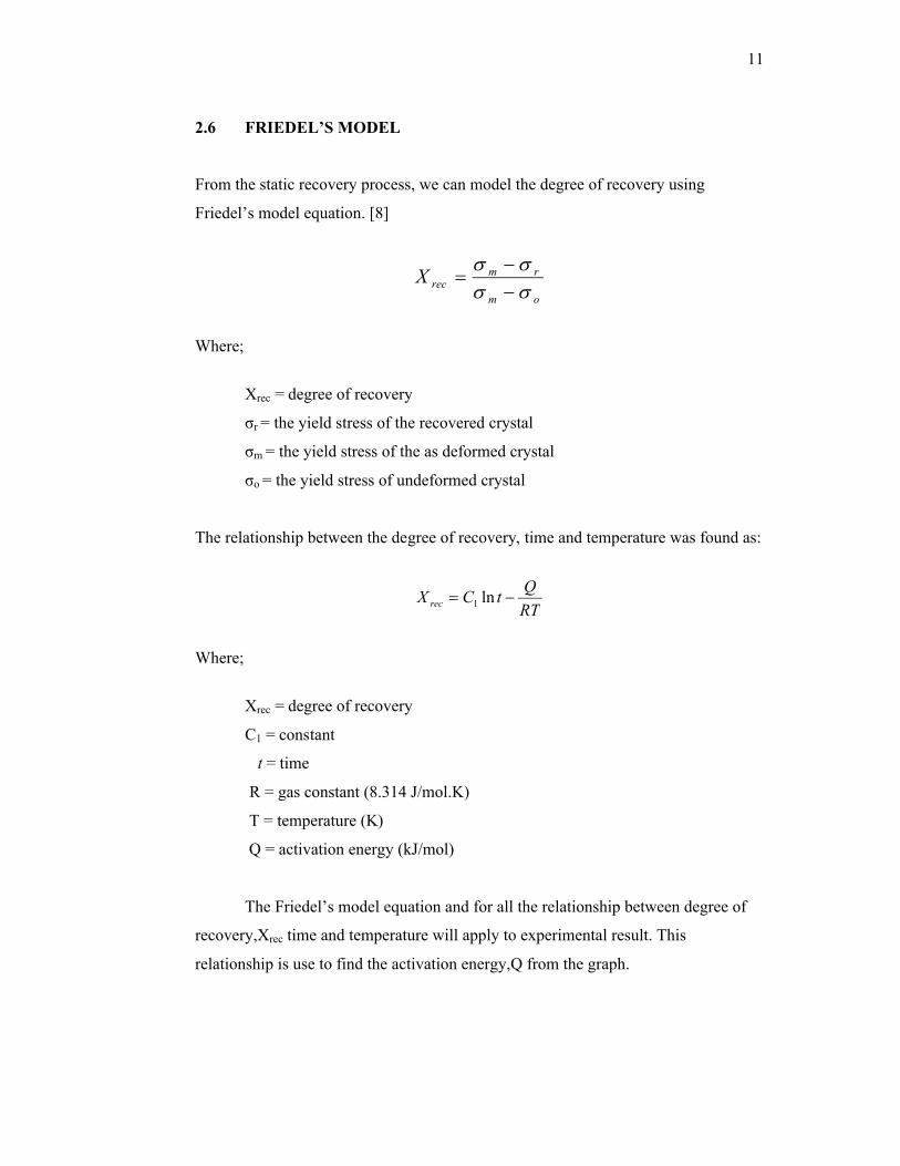
2.6 FRIEDEL’S MODEL

From the static recovery process, we can model the degree of recovery using

Friedel’s model equation. [8]

om

rmrecX

Where;

Xrec = degree of recovery

σr = the yield stress of the recovered crystal

σm = the yield stress of the as deformed crystal

σo = the yield stress of undeformed crystal

The relationship between the degree of recovery, time and temperature was found as:

RT

QtCX rec ln1

Where;

Xrec = degree of recovery

C1 = constant

t = time

R = gas constant (8.314 J/mol.K)

T = temperature (K)

Q = activation energy (kJ/mol)

The Friedel’s model equation and for all the relationship between degree of

recovery,Xrec time and temperature will apply to experimental result. This

relationship is use to find the activation energy,Q from the graph.

12

Figure 2.4: Determination of reloading flow stress and degree of softening

by the back extrapolation (be) and offset (os). [8]

2.7 REVERSE CALCULATION FROM PUBLISHED RESULT

From the journal E. Nes,Acta metall.metar.Recovery Revisited 43 (1994), the

Friedel’s model equation can be applied at graph Xrec Vs Time to find the value of

activation energy,Q.

Figure 2.5: Graph Xrec vs time with a different temperature. [9]

13

To find the value of activation energy,Q the value of recovery can be

measured at constant time (1 hour at red line) with a different temperatures

(100oC,200oC,300oC and 400oC). Then, the graph Xrec vs 1/Temperature can be

plotted.

Figure 2.6: Graph Xrec vs 1/Temperature.

From graph Xrec vs 1/T, the linear equation are plotted which is y = -62303x

+ 168.6. Then using Friedel’s model equation, the comparison can be made to find

the activation energy,Q.

y = mx + c

y = -62303x + 168.6 (1)

Applied Friedel’s model equation:

(2)RT

QtCX rec ln1

14

Then, made the comparison between equation (1) & (2) to find activation energy,Q:

62303R

Q

Q = 62303 x (8.314 J/mol.K)

= 517.987 kJ/mol.

Finally, this Q value from the literature review will used to compare with

experimental Q value.

xTR

Q62303

1

CHAPTER 3

METHODOLOGY

3.1 INTRODUCTION

In this chapter, detailed process about static recovery is presented. Start with

machining the specimens, annealing process and continue with compression test. In

annealing process we go through a different test which is against pre-strain,

temperature and time. Then the result from the compression test will use to validate

the Fridel’s model.

3.2 MACHINING PROCESS

Before we go through to a compression test, the specimens are started to be

made. The specimens needed in this project have a cylinder shape and must be made

around 50 specimens. The dimension for the diameter is 10mm while 25mm for the

length. To make this specimens, the aluminum material will go through a few

machining process.

3.2.1 Bandsaw

The raw material for aluminum alloys has a long dimension in length, so the

bandsaw machine is using to cut the material with desire dimension. The material

that we cut must have a tolerance (around +3mm), so the end of material can be

facing using a lathe machine.

16

Figure 3.1: Mechanical bandsaw

3.2.2 Lathe Machine

A lathe is a machine tool which turns cylindrical material, touches a cutting

tool to it, and cuts the material. The lathe is one of the machine tools most well used

by machining.

Figure 3.2: Mechanical lathe machine

17

There are some processes that involve during the specimen which is centre drill,

turning and facing.

1. Centre drill

Applied at both end surface of specimen to hold the work piece from

bending and vibrate.

2. Turning

This is a process to reduce the raw material dimension to become

10mm diameter of specimens.

3. Facing

This is a process to make a flat surface at the end of work piece and

the tolerance that we have at specimens can be cut to become our

desire length which is 25mm.

3.2.2.1 Three important element

In order to get an efficient process and beautiful surface at the lathe

machining, it is important to adjust a rotating speed, a cutting depth and a

sending speed.

Figure3.3: Lathe machine process

18

1. Rotating speed

It expresses with the number of rotations (rpm) of the chuck of a

lathe. When the rotating speed is high, processing speed becomes

quick, and a processing surface is finely finished. However, since a

little operation mistakes may lead to the serious accident, it is better to

set low rotating speed at the first stage.

2. Cutting Depth

The cutting depth of the tool affects to the processing speed and the

roughness of surface. When the cutting depth is big, the processing

speed becomes quick, but the surface temperature becomes high, and

it has rough surface. Moreover, a life of byte also becomes short. So,

it is better to set to small value.

3. Sending speed(feed)

The sending speed of the tool also affects to the processing speed and

the roughness of surface. When the sending speed is high, the

processing speed becomes quick. When the sending speed is low, the

surface is finished beautiful.

3.2.2.2 Precaution steps

1. Don't keep a chuck handle attached by the chuck. Next, it flies at the

moment of turning a lathe.

2. Don't touch the byte table into the rotating chuck. Not only a byte but

the table or the lathe is damaged.

19

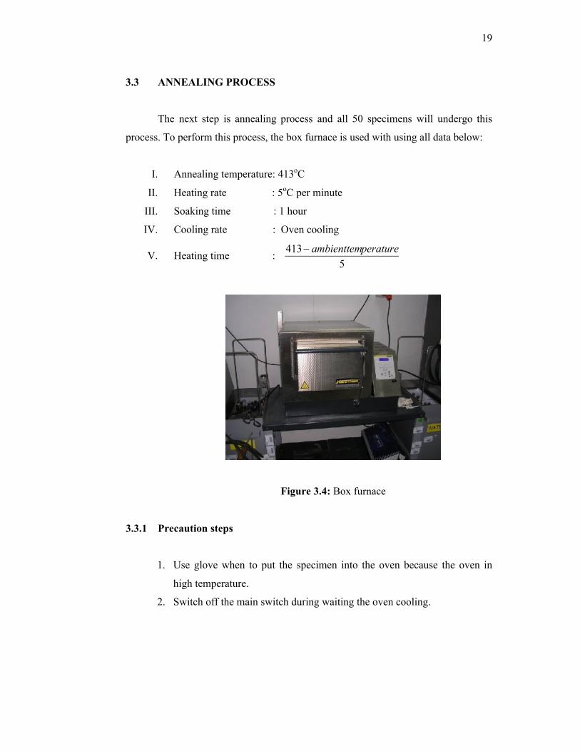
3.3 ANNEALING PROCESS

The next step is annealing process and all 50 specimens will undergo this

process. To perform this process, the box furnace is used with using all data below:

I. Annealing temperature: 413oC

II. Heating rate : 5oC per minute

III. Soaking time : 1 hour

IV. Cooling rate : Oven cooling

V. Heating time : 5

413 peratureambienttem

Figure 3.4: Box furnace

3.3.1 Precaution steps

1. Use glove when to put the specimen into the oven because the oven in

high temperature.

2. Switch off the main switch during waiting the oven cooling.

20

3.4 PRE-STRAIN THE SPECIMENS

In this process, the compression test machine is used to perform pre-strain for

all specimens. The yield strength and maximum strength of specimens will get from

this process. In this project, the maximum load that can be applied to compression

test is 50kN. So, the pre-strain value is varying with 2.5%, 5%, 7.5% and 10%. For a

different temperature and time, the pre-strain value applied just 5% only. Then for

each pre- strain, we are using 3 specimens to get the average value.

Figure 3.5: Compression test

3.5 RECOVERY PROCESS

This process is use to find the degree of recovery,X with different

temperature, time and pre-strain.

I. For different temperatures:

Varying temperature: 100oC, 150oC, 200oC and 250oC.

Recovery time : 1 hour

Heating rate : 5oC

21

II. For different time:

Varying recovery time: 1 hour, 2 hour, 3 hour and 4 hour.

Recovery temperature : 150oC

Heating rate : 5oC

III. For different pre-strain:

Recovery temperature: 150oC

Recovery time : 1 hour

Heating rate : 5oC

3.6 PRE-STRAIN RECOVERED SPECIMENS

In this process, the recovered specimens will pre-strain again to find the new

yield strength. The new yield strength is used to find degree of recovery,Xrec and all

the data will recorded using compression test machine. For a different pre-strain,

varying pre-strain with 2.5%, 5%, 7.5% and 10%. For a different temperature and

time, just 5% pre-strain was applied.

3.7 ANALYZING DATA

After collected the data such as yield strength, maximum strength and

recovery yield strength, we can find Xrec using equation below:

om

rmrecX

After that, we can plotted the graph using excel to find the relationship

between degree of recovery,Xrec with pre-strain, temperature and time.

22

3.8 APPLYING FRIEDEL’S MODEL

From the graph that we plotted, we can find the activation energy,Q using

relationship of equation below:

RT

QtCX rec ln1

3.9 COMPARISON

After we get the activation energy,Q from the plotted graph, we can compare

the Q value with a theory value of activation energy. From the comparison, we can

conclude weather we can validate the static recovery process using Friedel’s model

or not.

CHAPTER 4

RESULT AND DISCUSSION

4.1 INTRODUCTION

In this chapter, the result of relationship between degree of recovery,Xrec with

pre-strain, temperature and time are shown. The calculation of how to find the

activation energy,Q also will produce step by step. Then, some discussion is made

from the result to prove this project objective.

4.2 RESULT

From this experiment, 3 graphs can be plotted which is:

1. Degree of recovery,Xrec versus 1/Temperature at constant pre-strain 5% and

time for 1 hour.

2. Degree of recovery,Xrec versus lnt at constant pre-strain 5% and temperature

for 150oC.

3. Degree of recovery,Xrec versus pre-strain at constant time for 1 hour and

temperature for 150oC.

24

4.2.1 Relationship between Xrec vs 1/Temperature

The relationship between degree of recovery,Xrec and temperature can be

plotted using Friedel’s model equation. The data below has shown the characteristic

of softening before and after static recovery process using pre-strain 5% at different

temperature.

Table 4.1: Data for temperature 100oC at 5% and 1 hour

σo σm σr σm – σr σm - σo 1/T Xrec Xrec (%)

41.141 112.1 104.96 7.14 70.959 0.002681 0.100621 10.0621

39.5 111.2 106.2 5 71.7 0.002681 0.069735 6.9735

41.62 111.8 93.78 18.02 70.18 0.002681 0.256768 25.6768


σo σm σr σm – σr σm -σo 1/T Xrec Xrec (%)

22.83 112.9 97.199 15.701 90.07 0.002364 0.17432 17.432

43.49 110.7 97.72 12.98 67.21 0.002364 0.193126 19.3126

58.42 107.3 96.711 10.589 48.88 0.002364 0.216633 21.6633


σo σm σr σm – σr σm -σo 1/T Xrec Xrec (%)

46.9 113 77.558 35.442 66.1 0.002114 0.536188 53.6188

64.65 110.5 70.59 39.91 45.85 0.002114 0.870447 87.0447

45.11 111.9 68.64 43.26 66.79 0.002114 0.647702 64.7702

characterisation and modelling of...

Documents