chapter y: (0th level chapter heading)
TRANSCRIPT

Final Draft Technical Summary IPCC WG1 Fourth Assessment Report
1 2 3 4 5 6 7
Working Group I Contribution to the Intergovernmental Panel on Climate Change
Fourth Assessment Report
Climate Change 2007: The Physical Science Basis 8
9 10 11 12
Technical Summary 13
14 15 16 17 18 19 20 21 22 23 24 25 26 27 28 29 30 31 32 33 34 35 36 37 38 39 40
Coordinating Lead Authors: Susan Solomon (USA), Dahe Qin (China), Martin Manning (USA, New Zealand) Lead Authors: Richard Alley (USA), Terje Berntsen (Norway), Nathaniel L. Bindoff (Australia), Zhenlin Chen (China), Amnat Chidthaisong (Thailand), Jonathan Gregory (UK), Gabriele Hegerl (USA, Germany), Martin Heimann (Germany, Switzerland), Bruce Hewitson (South Africa), Brian Hoskins (UK), Fortunat Joos (Switzerland), Jean Jouzel (France), Vladimir Kattsov (Russia), Ulrike Lohmann (Switzerland), Taroh Matsuno (Japan), Mario Molina (USA, Mexico), Neville Nicholls (Australia), Jonathan Overpeck (USA), Graciela Raga (Mexico, Argentina), Venkatachalam Ramaswamy (USA), Jiawen Ren (China), Matilde Rusticucci (Argentina), Richard Somerville (USA), Thomas F. Stocker (Switzerland), Ronald J. Stouffer (USA), Penny Whetton (Australia), Richard A. Wood (UK), David Wratt (New Zealand) Contributing Authors: Julie Arblaster (USA, Australia), Guy Brasseur (USA, Germany), Jens Hesselbjerg Christensen (Denmark), Kenneth Denman (Canada), David Fahey (USA), Piers Forster (UK), James Haywood (UK), Eystein Jansen (Norway), Philip D. Jones (UK), Reto Knutti (Switzerland), Hervé Le Treut (France), Peter Lemke (Germany), Gerald Meehl (USA), David Randall (USA), Daíthí A. Stone (UK), Kevin E. Trenberth (USA), Jürgen Willebrand (Germany), Francis Zwiers (Canada) Review Editors: Kansri Boonpragob (Thailand), Filippo Giorgi (Italy), Bubu Pateh Jallow (The Gambia) Date of Draft: 27 October 2006
Do Not Cite or Quote TS-1 Total pages: 56

Final Draft Technical Summary IPCC WG1 Fourth Assessment Report
Table of Contents 1 2 3 4 5 6 7 8 9
10 11 12 13 14 15 16 17 18 19 20 21 22 23 24 25 26 27 28 29 30 31 32 33 34 35 36 37 38 39 40 41 42 43 44 45
TS.1 Introduction................................................................................................................................................................3
Box TS.1.1: Treatment of Uncertainties in the Working Group I Assessment ...........................................................3 TS.2 Changes in Human and Natural Drivers of Climate...................................................................................................5
TS.2.1 Greenhouse Gases.........................................................................................................................................5 TS.2.2 Aerosols......................................................................................................................................................10 TS.2.3 Aviation Contrails and Cirrus, Land Use, and Other Effects......................................................................10 TS.2.4 Radiative Forcing Due to Solar Activity and Volcanic Eruptions ..............................................................11 TS.2.5 Net Global Radiative Forcing, Global Warming Potentials, and Patterns of Forcing...............................12 TS 2.6 Surface Forcing and the Hydrologic Cycle.................................................................................................13
TS.3 Observations of Changes in Climate........................................................................................................................17 TS.3.1 Atmospheric Changes: Instrumental Record...............................................................................................17 Box TS.3.1: Patterns (modes) of Climate Variability ..............................................................................................19 TS.3.2 Changes in the Cryosphere: Instrumental Record ......................................................................................21 Box TS.3.2: Ice Sheet Dynamics and Stability .........................................................................................................23 TS.3.3 Changes in the Ocean: Instrumental Record ..............................................................................................24 Box TS.3.3: Sea Level ..............................................................................................................................................27 TS.3.4 Consistency Among Observations ...............................................................................................................28 Box.TS.3.4 Extreme Weather Events........................................................................................................................29 TS.3.5 A Paleoclimatic Perspective........................................................................................................................30 Box TS.3.5: Orbital Forcing ....................................................................................................................................32
TS.4 Understanding and Attributing Climate Change ......................................................................................................33 TS.4.1 Advances in Attribution of Changes in Global Scale Temperature in the Instrumental Period: Atmosphere, Ocean and Ice ..........................................................................................................................................................33 Box TS.4.1: Evaluation of Atmosphere-Ocean General Circulation Models ..........................................................34 TS.4.2 Attribution of Spatial and Temporal Changes in Temperature ...................................................................36 TS.4.3 Attribution of Changes in Circulation, Precipitation and Other Climate Variables...................................36 TS.4.4 Paleoclimate Studies of Attribution.............................................................................................................37 TS.4.5 Climate Response to Radiative Forcing......................................................................................................37
TS.5 Projections of Future Changes in Climate................................................................................................................38 Box TS.5.1: Hierarchy of Global Climate Models...................................................................................................39 TS.5.1 Understanding near Term Climate Change ................................................................................................40 Box TS.5.2: Committed Climate Change .................................................................................................................41 TS.5.2 Large Scale Projections for the 21st century ..............................................................................................41 TS.5.3 Regional Scale Projections .........................................................................................................................44 Box TS.5.3. Regional Downscaling..........................................................................................................................45 TS.5.4 Coupling Between Climate Change and Changes in Biogeochemical Cycles ............................................45 TS.5.5 Implications of Climate Processes and their Timescales for Long-Term Projections ................................47
TS.6 Robust Findings and Key Uncertainties...................................................................................................................48 TS.6.1 Changes in Human and Natural Drivers of Climate...................................................................................48 TS.6.2 Observations of Changes in Climate...........................................................................................................49 TS.6.3 Understanding and Attributing Climate Change ........................................................................................52 TS.6.4 Projections of Future Changes in Climate..................................................................................................53
Do Not Cite or Quote TS-2 Total pages: 56
Final Draft Technical Summary IPCC WG1 Fourth Assessment Report
TS.1 INTRODUCTION 1 2 3 4 5 6 7 8 9
10 11 12 13 14 15 16 17 18 19 20 21 22 23 24 25 26 27 28 29 30 31 32 33 34 35 36 37 38
In the last 6 years since the IPCC’s Third Assessment Report (TAR), significant progress has been made in understanding past and recent climate change and in projecting future changes. These advances have arisen from: large amounts of new data, more sophisticated analyses of data, improvements in the understanding and simulation of physical processes in climate models, and more extensive exploration of uncertainty ranges in model results. The increased confidence in climate science provided by these developments is evident in this Working Group I contribution to the IPCC’s Fourth Assessment Report. While this report provides new and important policy-relevant information on the scientific understanding of climate change, the complexity of the climate system and the multiple interactions that determine its behaviour impose limitations on our ability to understand fully the future course of Earth’s global climate. There is still an incomplete physical understanding of many components of the climate system and their role in climate change. Key uncertainties include aspects of the roles played by clouds, the cryosphere, the oceans, land-use, and couplings between climate and biogeochemical cycles. The areas of science covered in this report continue to undergo rapid progress and it should be recognized that the present assessment reflects scientific understanding based on the peer-reviewed literature available in mid-2006. The key findings of the IPCC Working Group I assessment are presented in the Summary for Policymakers. This Technical Summary provides a more detailed overview of the scientific basis for those findings and provides a road map to the chapters of the underlying report. It focuses on key findings, highlighting what is new since the TAR. The structure of the Technical Summary is as follows:
• Section 2: an overview of current scientific understanding of the natural and anthropogenic drivers of changes in climate;
• Section 3: an overview of observed changes in the climate system (including the atmosphere, oceans and cryosphere) and their relationships to physical processes;
• Section 4: an overview of explanations of observed climate changes based on climate models and physical understanding, the extent to which climate change can be attributed to specific causes, and a new evaluation of climate sensitivity to greenhouse gas increases;
• Section 5: an overview of projections for both near- and far-term climate changes including the time scales of responses to changes in forcing, and probabilistic information on future climate change;
• Section 6: a summary of the most robust findings and the remaining key uncertainties in current physical climate change science.
Each paragraph in the Technical Summary reporting substantive results is followed by a reference in curly brackets to the corresponding chapter section(s) of the underlying report where the detailed assessment of the scientific literature and additional information can be found.
39 BOX TS.1.1: TREATMENT OF UNCERTAINTIES IN THE WORKING GROUP I ASSESSMENT 40
The importance of consistent and transparent treatment of uncertainties is clearly recognized by the IPCC in 41 preparing its assessments of climate change. The increasing attention given to formal treatments of 42 uncertainty in previous assessments is addressed in Section 1.6. To promote consistency in the general 43 treatment of uncertainty across all three Working Groups, authors of the Fourth Assessment Report have 44 been asked to follow a brief set of guidance notes on determining and describing uncertainties in the context 45 of an assessment1. This box summarises the way in which those guidelines have been applied by Working 46 Group I and covers some aspects of the treatment of uncertainty specific to material assessed here. 47
48 Uncertainties can be classified in several different ways according to their origin. Two primary types are 49 value uncertainties and structural uncertainties. Value uncertainties arise from the incomplete determination 50 of particular values or results, e.g. when data are inaccurate or not fully representative of the phenomenon of 51 interest. Structural uncertainties arise from an incomplete understanding of the processes that control 52 particular values or results, e.g. when the conceptual framework or model used for analysis does not include 53 all the relevant processes or relationships. Value uncertainties are generally estimated using statistical 54
1 See Supplementary Material for this report Do Not Cite or Quote TS-3 Total pages: 56
Final Draft Technical Summary IPCC WG1 Fourth Assessment Report
techniques and expressed probabilistically. Structural uncertainties are generally described by giving the 1 authors’ collective judgment of their confidence in the correctness of a result. In both cases estimating 2 uncertainties is intrinsically about describing the limits to knowledge and for this reason involves expert 3 judgment about the state of that knowledge. A different type of uncertainty arises in systems that are either 4 chaotic or not fully deterministic in nature and this also limits our ability to project all aspects of climate 5 change. 6
7 The scientific literature assessed here uses a variety of other generic ways of categorizing uncertainties. 8 Uncertainties associated with random errors have the characteristic of decreasing as additional 9 measurements are accumulated, whereas those associated with systematic errors do not. In dealing with 10 climate records considerable attention has been given to the identification of systematic errors or unintended 11 biases arising from data sampling issues and methods of analysing and combining data. Specialized 12 statistical methods based on quantitative analysis have been developed for the detection and attribution of 13 climate change and for producing probabilistic projections of future climate parameters. These are 14 summarised in the relevant chapters. 15
16 The uncertainty guidance provided for the Fourth Assessment Report draws, for the first time, a careful 17 distinction between levels of confidence in our scientific understanding and the likelihoods of specific 18 results. This allows authors to express high confidence that an event is extremely unlikely (e.g., rolling a dice 19 twice and getting a six both times), as well as high confidence that an event is about as likely as not (e.g., a 20 tossed coin coming up heads). Confidence and likelihood as used here are distinct concepts but are often 21 linked in practice. 22
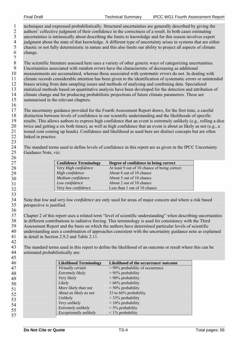
23 The standard terms used to define levels of confidence in this report are as given in the IPCC Uncertainty 24 Guidance Note, viz: 25
26 27
28 29 30 31
Confidence Terminology Degree of confidence in being correct Very High confidence At least 9 out of 10 chance of being correct High confidence About 8 out of 10 chance Medium confidence About 5 out of 10 chance Low confidence About 2 out of 10 chance Very low confidence Less than 1 out of 10 chance 32
33 Note that low and very low confidence are only used for areas of major concern and where a risk based 34 perspective is justified. 35 36 Chapter 2 of this report uses a related term “level of scientific understanding” when describing uncertainties 37 in different contributions to radiative forcing. This terminology is used for consistency with the Third 38 Assessment Report and the basis on which the authors have determined particular levels of scientific 39 understanding uses a combination of approaches consistent with the uncertainty guidance note as explained 40 in detail in Section 2.9.2 and Table 2.11. 41 42 The standard terms used in this report to define the likelihood of an outcome or result where this can be 43 estimated probabilistically are: 44 45
46 47 48 49 50 51 52 53 54 55
Likelihood Terminology Likelihood of the occurrence/ outcome Virtually certain > 99% probability of occurrence Extremely likely > 95% probability Very likely > 90% probability Likely > 66% probability More likely than not > 50% probability About as likely as not 33 to 66% probability Unlikely < 33% probability Very unlikely < 10% probability Extremely unlikely < 5% probability Exceptionally unlikely < 1% probability 57
Do Not Cite or Quote TS-4 Total pages: 56
Final Draft Technical Summary IPCC WG1 Fourth Assessment Report
The terms “Extremely likely/unlikely” and “More likely than not” as defined above have been added to 1 those given in the IPCC Uncertainty Guidance Note in order to provide a more specific assessment of 2 aspects including attribution and radiative forcing. 3
4 Unless noted otherwise, values given in this report are assessed best estimates and their uncertainty ranges 5 are 90% confidence intervals, i.e., there is an estimated 5% likelihood of the value being below the lower 6 end of the range or above the upper end of the range. Thus a value is very likely to lie in its given uncertainty 7 range. Note that in some cases the nature of the constraints on a value, or other information available, may 8 indicate an asymmetric distribution of the uncertainty range around a best estimate. In such cases the 9 uncertainty range is given in square brackets following the best estimate. 10
11 12 13 14 15 16 17 18 19 20 21 22 23 24 25 26 27 28 29 30 31 32 33 34 35 36 37 38 39 40 41 42 43 44 45 46 47 48 49 50 51 52
TS.2 CHANGES IN HUMAN AND NATURAL DRIVERS OF CLIMATE The Earth’s global mean climate is determined by incoming energy from the Sun and by the properties of the Earth and its atmosphere, namely the reflection, absorption, and emission of energy within the atmosphere and at the surface. Although changes in received solar energy (e.g., caused by variations in the Earth’s orbit around the Sun) inevitably affect the Earth’s energy budget, the properties of the atmosphere and surface are also important and these may be affected by climate feedbacks. The importance of climate feedbacks is evident in the nature of past climate changes as recorded in ice-cores up to 650,000 years old. Changes have occurred in several aspects of the atmosphere and surface that alter the global energy budget of the Earth and can therefore cause the climate to change. Among these are increases in greenhouse gas concentrations that act primarily to increase the atmospheric absorption of outgoing radiation, and increases in aerosols (microscopic airborne particles or droplets) that act to reflect and absorb incoming solar radiation and change cloud radiative properties. Such changes cause a radiative forcing of the climate system2. Forcing agents can differ considerably from one another in terms of the magnitudes of forcing, as well as spatial and temporal features. Positive and negative radiative forcings contribute to increases and decreases, respectively, in globally averaged surface temperature. This section updates the understanding of estimated anthropogenic and natural radiative forcings. The overall response of global climate to radiative forcing is complex due to a number of positive and negative feedbacks that can have a strong influence on the climate system (see e.g., Sections 4.5 and 5.4). Although water vapour is a strong greenhouse gas, its concentration in the atmosphere changes in response to changes in surface climate and these must be treated as a feedback effect and not as a radiative forcing. This section also summarises changes in the surface energy budget and its links to the hydrological cycle. Insights into the effects of agents such as aerosols on precipitation are also noted. TS.2.1 GREENHOUSE GASES The dominant factor in the radiative forcing of climate in the industrial era is the increasing concentration of various greenhouse gases in the atmosphere. Several of the major greenhouse gases occur naturally but increases in their atmospheric concentrations over the last 250 years are due largely to human activities. Other greenhouse gases are entirely the result of human activities. The contribution of each greenhouse gas to radiative forcing over a particular period of time is determined by the change in its concentration in the atmosphere over that period and the effectiveness of the gas in perturbing the radiative balance. Current atmospheric concentrations of the different greenhouse gases considered in this report vary by more than 8 orders of magnitude (factor of 108), and their radiative efficiencies vary by more than 4 orders of magnitude (factor of 104) reflecting the enormous diversity in their properties and origins. The current concentration of a greenhouse gas in the atmosphere is the net result of the history of its past emissions and removals from the atmosphere. The gases and aerosols considered here are emitted to the atmosphere by human activities or are formed from precursor species emitted to the atmosphere. These
2 Radiative forcing is a measure of the influence a factor has in altering the balance of incoming and outgoing energy in the Earth-atmosphere system and is an index of the importance of the factor as a potential climate change mechanism. In this report radiative forcing values are for changes relative to a pre-industrial background for 1750, are expressed in Watts per square meter (W m–2) and, unless otherwise noted, refer to a global and annual average value. See Glossary for further details. Do Not Cite or Quote TS-5 Total pages: 56
Final Draft Technical Summary IPCC WG1 Fourth Assessment Report
1 2 3 4 5 6 7 8 9
10 11 12 13 14 15 16 17 18 19 20 21 22 23 24 25 26 27 28 29 30 31 32 33 34 35 36 37 38 39 40 41 42 43 44 45 46 47 48 49 50 51 52 53 54 55 56 57
emissions are offset by chemical and physical removal processes. With the important exception of CO2, it is generally the case that these processes remove a specific fraction of the amount of a gas in the atmosphere each year and the inverse of this removal rate gives the mean lifetime for that gas. In some cases the removal rate may vary with gas concentration or other atmospheric properties, e.g. temperature or background chemical conditions. Long-lived greenhouse gases (LLGHGs), e.g. carbon dioxide, methane, and nitrous oxide, are chemically stable and persist in the atmosphere over time scales of a decade to centuries or longer, so that their emission has a long-term influence on climate. Because these gases are long-lived they become well-mixed throughout the atmosphere much faster than they are removed and their global concentrations can be accurately estimated from data at a few locations. Carbon dioxide (CO2) does not have a specific lifetime because it is continuously cycled between the atmosphere, oceans and land biosphere and its net removal from the atmosphere involves a range of processes with different timescales. Short-lived gases, e.g. sulphur dioxide and carbon monoxide, are chemically reactive and generally removed by natural oxidation processes in the atmosphere, by removal at the surface, or by washout in precipitation; their concentrations are hence highly variable. Ozone is a significant greenhouse gas that is formed and destroyed by chemical reactions involving other species in the atmosphere. In the troposphere, the human influence on ozone occurs primarily through changes in precursor gases that lead to its formation, while in the stratosphere, the human influence has been primarily through changes in ozone removal rates caused by chlorofluorocarbons (CFCs) and other ozone-depleting substances. TS.2.1.1 Changes in Atmospheric Carbon Dioxide, Methane, and Nitrous Oxide Current concentrations of atmospheric CO2 and methane (CH4) far exceed pre-industrial values found in polar ice core records of atmospheric composition dating back 650,000 years. Multiple lines of evidence confirm that the post-industrial rise in these gases does not stem from natural mechanisms (see Figure TS-1 and Figure TS-2). {2.3, 6.3, 6.4, 6.5, FAQ 7.1} [INSERT FIGURE TS-1 HERE] The total radiative forcing of the Earth's climate due to increases in the concentrations of the LLGHGs CO2, methane (CH4), and nitrous oxide (N2O), and very likely the rate of increase in the total forcing due to these gases over the period since 1750 are unprecedented in more than 10,000 years (Figure TS-2). It is very likely that the sustained rate of increase in the combined radiative forcing from these greenhouse gases of about 1 W m-2 over the past four decades is at least six times faster than at any time during the two millennia before the Industrial Era, the period for which ice core data have the required temporal resolution. The radiative forcing due to these long-lived greenhouse gases has the highest level of confidence of any forcing agent. {2.3, 6.4} [INSERT FIGURE TS-2 HERE] The concentration of atmospheric CO2 has increased from a pre-industrial value of about 280 ppm to 379 ppm in 2005. Atmospheric CO2 concentration increased by only 20 ppm over the 8,000 years prior to industrialization; multi-decadal to centennial scale variations were less than 10 ppm and likely due mostly to natural processes. However, since 1750, the CO2 concentration has risen by nearly 100 ppm. The annual CO2 growth-rate was larger during the last 10 years (1995–2005 average: 1.9 ppm yr–1), than it has been since continuous direct atmospheric measurements began (1960–2005 average: 1.4 ppm yr-1). {2.3, 6.4, 6.5} Increases in atmospheric CO2 since pre-industrial times are responsible for a radiative forcing of 1.66 ± 0.17 W m–2; a contribution which dominates all other radiative forcing agents considered in this report. For the 1995–2005 decade, the growth rate of CO2 in the atmosphere led to a 20% increase in its radiative forcing. {2.3, 6.4, 6.5} Emissions of CO2 from fossil fuel use and from the effects of land-use change (LUC) on plant and soil carbon are the primary sources of increased atmospheric CO2. Since 1750, it is estimated that about 65% of anthropogenic CO2 emissions have come from fossil fuel burning and about 35% from land use change.
Do Not Cite or Quote TS-6 Total pages: 56
Final Draft Technical Summary IPCC WG1 Fourth Assessment Report
About 45% of this CO2 has remained in the atmosphere, while about 30% has been taken up by the oceans and the remainder has been taken up by the terrestrial biosphere. About half of a CO
1 2 3 4 5 6 7 8 9
10 11 12 13 14 15 16 17 18 19 20
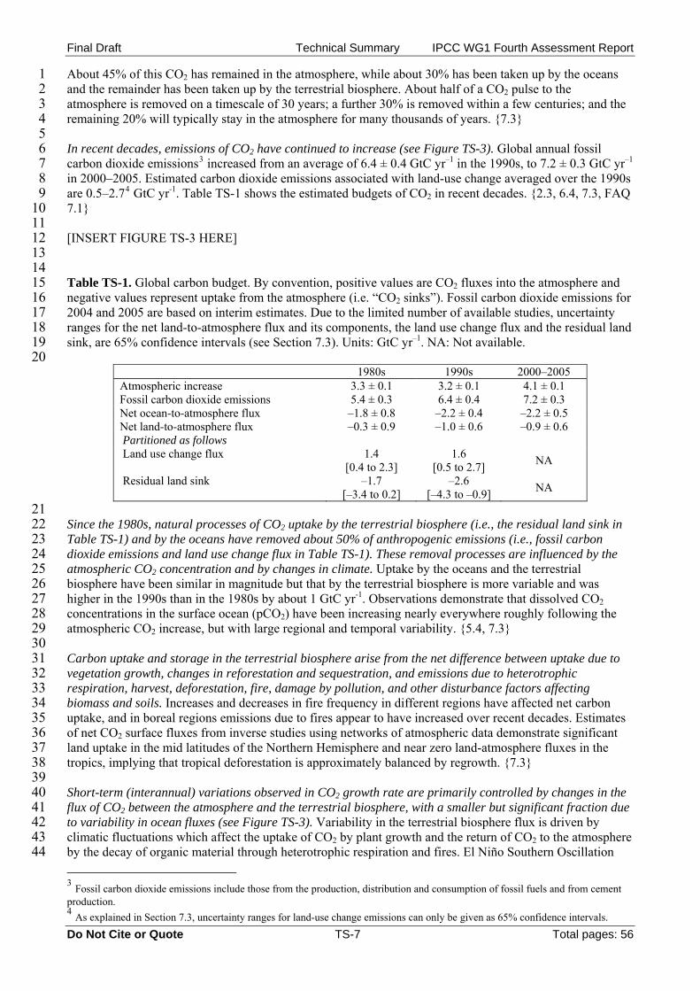
2 pulse to the atmosphere is removed on a timescale of 30 years; a further 30% is removed within a few centuries; and the remaining 20% will typically stay in the atmosphere for many thousands of years. {7.3} In recent decades, emissions of CO2 have continued to increase (see Figure TS-3). Global annual fossil carbon dioxide emissions3 increased from an average of 6.4 ± 0.4 GtC yr–1 in the 1990s, to 7.2 ± 0.3 GtC yr–1
in 2000–2005. Estimated carbon dioxide emissions associated with land-use change averaged over the 1990s are 0.5–2.74 GtC yr-1. Table TS-1 shows the estimated budgets of CO2 in recent decades. {2.3, 6.4, 7.3, FAQ 7.1} [INSERT FIGURE TS-3 HERE] Table TS-1. Global carbon budget. By convention, positive values are CO2 fluxes into the atmosphere and negative values represent uptake from the atmosphere (i.e. “CO2 sinks”). Fossil carbon dioxide emissions for 2004 and 2005 are based on interim estimates. Due to the limited number of available studies, uncertainty ranges for the net land-to-atmosphere flux and its components, the land use change flux and the residual land sink, are 65% confidence intervals (see Section 7.3). Units: GtC yr–1. NA: Not available.
1980s 1990s 2000–2005 Atmospheric increase 3.3 ± 0.1 3.2 ± 0.1 4.1 ± 0.1 Fossil carbon dioxide emissions 5.4 ± 0.3 6.4 ± 0.4 7.2 ± 0.3 Net ocean-to-atmosphere flux –1.8 ± 0.8 –2.2 ± 0.4 –2.2 ± 0.5 Net land-to-atmosphere flux –0.3 ± 0.9 –1.0 ± 0.6 –0.9 ± 0.6 Partitioned as follows Land use change flux 1.4
[0.4 to 2.3] 1.6
[0.5 to 2.7] NA
Residual land sink –1.7 [–3.4 to 0.2]
–2.6 [–4.3 to –0.9] NA
21 22 23 24 25 26 27 28 29 30 31 32 33 34 35 36 37 38 39 40 41 42 43 44
Since the 1980s, natural processes of CO2 uptake by the terrestrial biosphere (i.e., the residual land sink in Table TS-1) and by the oceans have removed about 50% of anthropogenic emissions (i.e., fossil carbon dioxide emissions and land use change flux in Table TS-1). These removal processes are influenced by the atmospheric CO2 concentration and by changes in climate. Uptake by the oceans and the terrestrial biosphere have been similar in magnitude but that by the terrestrial biosphere is more variable and was higher in the 1990s than in the 1980s by about 1 GtC yr-1. Observations demonstrate that dissolved CO2 concentrations in the surface ocean (pCO2) have been increasing nearly everywhere roughly following the atmospheric CO2 increase, but with large regional and temporal variability. {5.4, 7.3} Carbon uptake and storage in the terrestrial biosphere arise from the net difference between uptake due to vegetation growth, changes in reforestation and sequestration, and emissions due to heterotrophic respiration, harvest, deforestation, fire, damage by pollution, and other disturbance factors affecting biomass and soils. Increases and decreases in fire frequency in different regions have affected net carbon uptake, and in boreal regions emissions due to fires appear to have increased over recent decades. Estimates of net CO2 surface fluxes from inverse studies using networks of atmospheric data demonstrate significant land uptake in the mid latitudes of the Northern Hemisphere and near zero land-atmosphere fluxes in the tropics, implying that tropical deforestation is approximately balanced by regrowth. {7.3} Short-term (interannual) variations observed in CO2 growth rate are primarily controlled by changes in the flux of CO2 between the atmosphere and the terrestrial biosphere, with a smaller but significant fraction due to variability in ocean fluxes (see Figure TS-3). Variability in the terrestrial biosphere flux is driven by climatic fluctuations which affect the uptake of CO2 by plant growth and the return of CO2 to the atmosphere by the decay of organic material through heterotrophic respiration and fires. El Niño Southern Oscillation
3 Fossil carbon dioxide emissions include those from the production, distribution and consumption of fossil fuels and from cement production. 4 As explained in Section 7.3, uncertainty ranges for land-use change emissions can only be given as 65% confidence intervals.
Do Not Cite or Quote TS-7 Total pages: 56

Final Draft Technical Summary IPCC WG1 Fourth Assessment Report
1 2 3 4 5 6 7 8 9
10 11 12 13 14 15 16 17 18 19 20 21 22 23 24 25 26 27 28 29 30 31 32 33 34 35 36 37 38 39 40 41 42 43 44 45 46 47 48 49 50 51 52 53 54 55 56 57
(ENSO) events are a major source of inter-annual variability in CO2 growth rates due to their effects on fluxes through land and sea-surface temperatures, precipitation, and the incidence of fires. {7.3} The direct effects of increasing atmospheric CO2 on terrestrial carbon uptake on a large scale cannot be quantified reliably at present. Plant growth can be stimulated by increased atmospheric CO2 concentrations and by nutrient deposition (fertilization effects). However, most experiments and studies show that such responses appear to be relatively short lived and strongly coupled to other effects such as availability of water and nutrients. Likewise, experiments and studies of the effects of climate (temperature and moisture) on heterotrophic respiration of litter and soils are equivocal. Note that the effect of climate change on carbon uptake is dealt with separately in section TS.5.4. {7.3} The methane abundance in 2005 of about 1774 ppb is more than double its pre-industrial value. Atmospheric methane concentrations varied slowly between 580 and 730 ppb over the last 10,000 years, but increased by about 1000 ppb in the last two centuries, representing the fastest changes in this gas over at least the last 80,000 years. In the late 1970s and early 1980s methane growth rates displayed maxima above 1% yr-1 but since the early 1990s have decreased significantly and were close to zero for the 6-year period from 1999 to 2005. Increases in methane abundance occur when emissions exceed removals. The recent decline in growth rates implies that emissions now approximately match removals, which are due primarily to oxidation by the hydroxyl radical (OH). Since the TAR, new studies using two independent tracers (methyl chloroform and 14CO) suggest no significant long-term change in the global abundance of OH. Thus the slow down in atmospheric methane growth rate since about 1993 is likely due to the atmosphere approaching an equilibrium during a period of near-constant total emissions . {2.3, 7.4, FAQ 7.1} Increases in atmospheric methane concentrations since preindustrial times have contributed a radiative forcing of 0.48 ± 0.05 W m-2. Among greenhouse gases this forcing remains second only to that of CO2 in magnitude. {2.3} Current methane levels are due to continuing anthropogenic emissions of methane, which are greater than natural emissions. Total methane emissions can be well determined from observed concentrations and independent estimates of removal rates. Emissions from individual sources of methane are not as well quantified as the total emissions but are mostly biogenic and include wetlands, ruminant animals, rice agriculture and biomass burning, with smaller contributions from industrial sources including fossil fuel-related emissions. {2.3, 6.4, 7.4} In addition to its slowdown over the last 15 years, the growth rate of atmospheric methane has shown high interannual variability, which is not yet fully explained. The largest contributions to interannual variability during the 1996–2001 period appear to be variations in emissions from wetlands and biomass burning. Several studies indicate that wetland methane emissions are highly sensitive to temperature and are also affected by hydrological changes. Available model estimates all indicate increases in wetland emissions due to future climate change but vary widely in the magnitude of such a positive feedback effect. {7.4} The nitrous oxide concentration in 2005 was 319 ppb, about 18% higher than its pre-industrial value. Nitrous oxide increased approximately linearly by about 0.8 ppb yr–1 for the past few decades. Ice core data show that the atmospheric concentration of N2O varied by less than about 10 ppb for 11,500 years before the onset of the industrial period. {2.3, 6.4, 6.5} The increase in nitrous oxide since the pre-industrial era now contributes a radiative forcing of 0.16 ± 0.02 W m–2 and is due primarily to human activities, particularly agriculture and associated land use change. Current estimates are that about 40% of total N2O emissions are anthropogenic but individual source estimates remain subject to significant uncertainties. {2.3, 7.4} TS.2.1.3 Changes in Atmospheric Halocarbons, Stratospheric Ozone, Tropospheric Ozone and Other
Gases CFCs and HCFCs are greenhouse gases that are purely anthropogenic in origin and used in a wide variety of applications. Emissions of these gases have decreased due to their phaseout under the Montreal Protocol and the concentrations of CFC-11 and CFC-113 are now decreasing due to natural removal processes.
Do Not Cite or Quote TS-8 Total pages: 56
Final Draft Technical Summary IPCC WG1 Fourth Assessment Report
1 2 3 4 5 6 7 8 9
10 11 12 13 14 15 16 17 18 19 20 21 22 23 24 25 26 27 28 29 30 31 32 33 34 35 36 37 38 39 40 41 42 43 44 45 46 47 48 49 50 51 52 53 54 55 56 57
Observations in polar firn cores since the TAR have now extended the available time series information for some of these greenhouse gases. Ice core and in-situ data confirm that industrial sources are the cause of observed increases in CFCs and HCFCs. {2.3} The Montreal Protocol gases contributed 0.32 ± 0.03 W m–2 to direct radiative forcing in 2005 with CFC-12 continuing to be the third most important long-lived radiative forcing agent. These gases as a group contribute about 12% of the total forcing due to LLGHGs. {2.3} The concentrations of industrial fluorinated gases covered by the Kyoto Protocol (HFCs, PFCs, SF6) are relatively small but are increasing rapidly. Their total radiative forcing in 2005 was 0.017 W m–2. {2.3} Tropospheric ozone is a short-lived greenhouse gas produced by chemical reactions of precursor species in the atmosphere and with large spatial and temporal variability. Improved measurements and modelling have advanced the understanding of chemical precursors that lead to the formation of tropospheric ozone, including carbon monoxide, nitrogen oxides (including sources and possible long-term trends in lightning) and formaldehyde. Overall, current models are successful in describing the principal features of the present global tropospheric ozone distribution on the basis of underlying processes. New satellite and in-situ measurements provide important global constraints for these models; however, there is less confidence in their ability to reproduce the changes in ozone associated with large changes in emissions or climate, and in the simulation of observed long-term trends in ozone concentrations over the 20th century. {7.4} Tropospheric ozone radiative forcing is estimated to be 0.35 [+0.25 to +0.65] W m–2 with a medium level of scientific understanding. The best-estimate of this radiative forcing has not changed since the TAR. Observations show that trends in tropospheric ozone during the last few decades vary in sign and magnitude at many locations, but there are indications of significant upward trends at low latitudes. Model studies of the radiative forcing due to the increase in tropospheric ozone since preindustrial times have increased in complexity and comprehensiveness compared with models used in the TAR. {2.3, 7.4} Changes in tropospheric ozone are linked to air quality and climate change. A number of studies have shown that summer daytime ozone concentrations correlate strongly with temperature. This correlation appears to reflect contributions from temperature-dependent biogenic volatile organic carbon emissions, thermal decomposition of peroxyacetylnitrate, which acts as a reservoir for NOx, and association of high temperatures with regional stagnation. Anomalously hot and stagnant conditions in the summer of 1988 were responsible for the highest surface-level ozone year on record in the northeastern United States. The summer heat wave in Europe in 2003 was also associated with exceptionally high local ozone at the surface. {Box 7.4} The radiative forcing due to the destruction of stratospheric ozone is caused by the Montreal Protocol gases and is re-evaluated to be –0.05 ± 0.10 W m–2, weaker than in the TAR, with a medium level of scientific understanding. The trend of greater and greater depletion of global stratospheric ozone observed during the 1980s and 1990s is no longer occurring; however, global stratospheric ozone is still about 4% below pre-1980 values and it is not yet clear whether ozone recovery has begun. In addition to the chemical destruction of ozone, dynamical changes may have contributed to Northern Hemisphere mid-latitude ozone reduction. {2.3} Direct emission of water vapour by human activities makes a negligible contribution to radiative forcing. However, as global mean temperatures increase, tropospheric water vapour concentrations increase and this represents a key feedback but not a forcing of climate change. Direct emission of water to the atmosphere by anthropogenic activities, mainly irrigation, is a possible forcing factor but corresponds to less than 1% of the natural sources of atmospheric water vapour. The direct injection of water vapour into the atmosphere from fossil fuel combustion is significantly lower than that from agricultural activity. {2.5} Based on chemical transport model studies, the radiative forcing from increases in stratospheric water vapour due to oxidation of methane is estimated to be +0.07 ± 0.05 W m–2. The level of scientific understanding is low because methane's contribution to the corresponding vertical structure of the water vapour change near the tropopause is uncertain. Other potential human causes of stratospheric water vapour increases that could contribute to radiative forcing are poorly understood. {2.3}
Do Not Cite or Quote TS-9 Total pages: 56
Final Draft Technical Summary IPCC WG1 Fourth Assessment Report
1 2 3 4 5 6 7 8 9
10 11 12 13 14 15 16 17 18 19 20 21 22 23 24 25 26 27 28 29 30 31 32 33 34 35 36 37 38 39 40 41 42 43 44 45 46 47 48 49 50 51 52 53 54 55 56 57
TS.2.2 AEROSOLS Direct aerosol radiative forcing is now considerably better quantified than previously and represents a major advance in our understanding since the time of the TAR when several components had a very low level of scientific understanding. A total direct aerosol radiative forcing combined across all aerosol types can now be given for the first time as –0.5 ± 0.4 W m–2, with a medium-low level of scientific understanding.Atmospheric models have improved and many now represent all aerosol components of significance. Aerosols vary considerably in their properties which affect the extent to which they absorb and scatter radiation, and thus different types may have a net cooling or warming effect. Industrial aerosol consisting mainly of a mixture of sulphates, organic and black carbon, nitrates, and industrial dust is clearly discernible over many continental regions of the Northern Hemisphere. Improved in situ, satellite and surface-based measurements (see Figure TS-4) have enabled verification of global aerosol model simulations. These improvements allow quantification of the total direct aerosol radiative forcing for the first time, representing an important advance since the TAR. The direct radiative forcing for individual species remains less certain and is estimated from models to be: sulphate –0.4 ± 0.2 W m–2, fossil-fuel organic carbon –0.05 ± 0.05 W m–2, fossil-fuel black carbon +0.2 ± 0.15 W m–2, biomass burning +0.05 ± 0.13 W m –2, nitrate –0.1 ± 0.1 W m–2, mineral dust –0.1 ± 0.2 W m–2. Two recent emission inventory studies support data from ice cores and suggest that global anthropogenic sulphate emissions decreased over the 1980–2000 period and that the geographic distribution of sulphate forcing has also changed. {2.4, 6.6}
[INSERT FIGURE TS-4 HERE] Significant changes in the estimates of the direct radiative forcing due to biomass burning, nitrate and mineral dust aerosols have occurred since the TAR. For biomass burning aerosol the estimated direct radiative forcing is now revised from being negative to near zero due to the estimate being strongly influenced by the occurrence of these aerosols over clouds. For the first time, radiative forcings due to nitrate aerosol is given. For mineral dust, the range in the direct radiative forcing is reduced due to a reduction in the estimate of its anthropogenic fraction. {2.4} Anthropogenic aerosol effects on water clouds cause an indirect cloud albedo effect (referred to as the first indirect effect in the TAR) which has a best estimate for the first time of –0.7 W m–2 [–0.3 to –1.8] W m-2. The number of global model estimates of the albedo effect for liquid water clouds has increased substantially since the TAR, and the estimates have been evaluated in a more rigorous way. The estimate for this radiative forcing comes from multiple model studies incorporating more aerosol species and describing aerosol-cloud interaction processes in greater detail. Model studies including more aerosol species or constrained by satellite observations tend to yield a relatively weaker cloud albedo effect. Despite the advances and progress since the TAR and the reduction in the spread of the estimate of the forcing, there remain large uncertainties in both measurements and modeling of processes, leading to a low level of scientific understanding, which is an elevation from the very low rank in the TAR. {2.4, 7.5, 9.2} Other effects of aerosol include a cloud lifetime effect, semi-direct effect, and aerosol-ice cloud interactions. These are considered to be part of the climate response rather than radiative forcings. {2.4, 7.5} TS.2.3 AVIATION CONTRAILS AND CIRRUS, LAND USE, AND OTHER EFFECTS Persistent linear contrails from global aviation contribute a small radiative forcing of 0.01 [+0.003 to +0.03] W m–2, with a low level of scientific understanding. This best-estimate is smaller than the estimate in the TAR. This difference results from new observations of contrail cover and reduced estimates of contrail optical depth. No best estimates are available for the net forcing from spreading contrails. Their effects on cirrus cloudiness and the global effect of aviation aerosol on background cloudiness remain unknown. {2.6} Human induced changes to land-cover have increased the global surface albedo, leading to a radiative forcing of –0.2 ± 0.2 Wm-2, the same as in the TAR, with a medium-low level of scientific understanding. Black carbon aerosols deposited on snow reduce the surface albedo and are estimated to yield an associated radiative forcing of +0.1 ±0.1 W m-2, with a low level of scientific understanding. Since the TAR, a number of estimates of the forcing from land-use changes have been made, using better techniques, exclusion of
Do Not Cite or Quote TS-10 Total pages: 56

Final Draft Technical Summary IPCC WG1 Fourth Assessment Report
1 2 3 4 5 6 7 8 9
10 11 12 13 14 15 16 17 18 19 20 21 22 23 24 25 26 27 28 29 30 31 32 33 34 35 36 37 38 39 40 41 42 43 44 45 46 47 48 49 50 51 52 53 54 55 56 57
feedbacks in the evaluation and improved incorporation of large-scale observations. Uncertainties in the estimate include mapping and characterization of present-day vegetation and historical state, parameterization of surface radiation processes, and biases in models' climate variables. The presence of soot particles in snow leads to a decrease in the albedo of snow and a positive forcing, and could affect snowmelt. Uncertainties are large regarding the manner in which soot is incorporated in snow and the resulting optical properties. {2.5} The impacts of land-use change on climate are expected to be locally significant in some regions, but are small at the global scale in comparison with greenhouse gas warming. Changes in the land surface (vegetation, soils, water) resulting from human activities can significantly affect local climate through shifts in radiation, cloudiness, surface roughness, and surface temperatures. Changes in vegetation cover can also have a substantial effect on surface energy and water balance at the regional scale. These effects involve non-radiative processes (implying that they cannot be quantified by a radiative forcing), and have a very low level of scientific understanding. {2.5, 7.2, 9.3, Box 11.4} The release of heat from anthropogenic energy production can be significant over urban areas but is not significant globally. {2.5} TS.2.4 RADIATIVE FORCING DUE TO SOLAR ACTIVITY AND VOLCANIC ERUPTIONS Continuous monitoring of total solar irradiance now covers the last 28 years. The data show a well-established 11-year cycle of 0.08% from solar cycle minima to maxima, with no significant long-term trend. New data have more accurately quantified changes in solar spectral fluxes over a broad range of wavelengths in association with changing solar activity. Improved calibrations using high-quality overlapping measurements have also contributed to a better understanding. Current understanding of solar physics and the known sources of irradiance variability suggest comparable irradiance levels during the past two solar cycles, including at solar minima. The primary known cause of contemporary irradiance variability is the presence on the Sun’s disk of sunspots (compact, dark features where radiation is locally depleted) and faculae (extended bright features where radiation is locally enhanced).{2.7} The estimated direct radiative forcing due to changes in the solar output since 1750 is 0.12 [range 0.06 to 0.3] W m–2 which is less than half of the estimate given in the TAR, with a low level of scientific understanding. The reduced radiative forcing estimate comes from a re-evaluation of the long-term change in solar irradiance since 1610 (the Maunder Minimum) based upon: a new reconstruction using a model of solar magnetic flux variations that does not invoke geomagnetic, cosmogenic or stellar proxies; improved understanding of recent solar variations and its relationship to physical processes; and re-evaluation of the variations of Sun-like stars. While this leads to an elevation in the level of scientific understanding from very low in the TAR to low now, uncertainties remain large because of the lack of direct observations and incomplete understanding of solar variability mechanisms on long time scales. {2.7, 6.6} Empirical associations have been reported between solar-modulated cosmic ray ionization of the atmosphere and globally-averaged low-level cloud cover but evidence for a systematic indirect solar effect remains ambiguous. It has been suggested that galactic cosmic rays with sufficient energy to reach the troposphere could alter the population of cloud condensation nuclei and hence microphysical cloud properties (droplet number and concentration), inducing changes in cloud processes analogous to the indirect cloud albedo effect of tropospheric aerosols and thus cause an indirect solar forcing of climate. Studies have probed various correlations with clouds in particular regions or using limited cloud types or limited time periods; however,the cosmic ray time series does not appear to correspond to global total cloud cover after 1991 or to global low-level cloud cover after 1994. Together with the lack of a proven physical mechanism and the plausibility of other causal factors affecting changes in cloud cover, this makes the association between galactic cosmic ray-induced changes in aerosol and cloud formation controversial. {2.7} Explosive volcanic eruptions greatly increase the concentration of stratospheric sulphate aerosols. A single eruption can thereby cool global mean climate for a few years. Volcanic aerosols perturb both the stratosphere and surface troposphere radiative energy budgets and climate in an episodic manner, and many past events are evident in ice core observations of sulphate as well as temperature records. There have been no explosive volcanic events since the 1991 Pinatubo eruption capable of injecting significant material to the
Do Not Cite or Quote TS-11 Total pages: 56

Final Draft Technical Summary IPCC WG1 Fourth Assessment Report
1 2 3 4 5 6 7 8 9
10 11 12 13 14 15 16 17 18 19 20 21 22 23 24 25 26 27 28 29 30 31 32 33 34 35 36 37 38 39 40 41 42 43 44 45 46 47 48 49 50 51 52 53 54 55 56 57
stratosphere. However, the potential exists for volcanic eruptions much larger than the 1991 Pinatubo eruption, which could produce larger radiative forcing and longer-term cooling of the climate system. {2.7, 6.4, 6.6, 9.2} TS.2.5 NET GLOBAL RADIATIVE FORCING, GLOBAL WARMING POTENTIALS, AND PATTERNS OF FORCING The understanding of anthropogenic warming and cooling influences on climate has improved since the TAR, leading to very high confidence that the effect of human activities since 1750 has been a net positive forcing of +1.6 [+0.6 to +2.4] W m-2, and it has likely been at least five times greater than that due to solar output changes. Improved understanding and better quantification of the forcing mechanisms since the TAR make it possible to derive a combined net anthropogenic radiative forcing for the first time. Taking together the component values for each forcing agent and their uncertainties yields the probability distribution of the combined anthropogenic radiative forcing estimate shown in Figure TS-5; the most likely value far exceeds the estimated radiative forcing from changes in solar output. Since the range in the estimate is +0.6 to +2.4 W m-2, there is very high confidence in the net positive radiative forcing of the climate system due to human activity. The LLGHGs together contribute +2.63 ± 0.26 W m-2, which is the dominant radiative forcing term and has the highest level of scientific understanding. In contrast, the total direct aerosol, cloud albedo and surface albedo effects that contribute negative forcings are less well understood and have larger uncertainties. The range in the net estimate is increased by the negative forcing terms which have larger uncertainties than the positive terms. The nature of the uncertainty in the estimated cloud albedo effect introduces a noticeable asymmetry in the distribution. Uncertainties in the distribution include structural aspects (e.g., representation of extremes in the component values, absence of any weighting of the RF mechanisms, possibility of unaccounted for but as yet unquantified radiative forcings) and statistical aspects (e.g., assumptions about the types of distributions describing component uncertainties). {2.7, 2.9} [INSERT FIGURE TS-5 HERE] The Global Warming Potential (GWP) is a useful metric for comparing the potential climate impact of the emissions of different LLGHGs (see Table TS-2). GWPs compare the integrated radiative forcing over a specified period (e.g., 100 years) from a unit mass pulse emission and are a way of comparing the potential climate change associated with emissions of different greenhouse gases. There are well-documented shortcomings of the GWP concept, particularly in using it to assess the impact of short-lived species. {2.10} [INSERT TABLE TS-2 HERE] For the magnitude and range of realistic forcings considered, evidence suggests an approximately linear relationship between global mean radiative forcing and global mean surface temperature response. The spatial patterns of radiative forcing vary between different forcing agents. However, the spatial signature of the climate response is not generally expected to match that of the forcing. Spatial patterns of climate response are largely controlled by climate processes and feedbacks. For example, sea ice albedo feedbacks tend to enhance the high-latitude response. Spatial patterns of response are also affected by differences in thermal inertia between land and sea areas. {2.8, 9.2} The pattern of response to a radiative forcing can be altered substantially if its structure is favourable for affecting a particular aspect of the atmospheric structure or circulation. Modelling studies and data comparisons suggest that mid- to high-latitude circulation patterns are likely to be affected by some forcings such as volcanic eruptions, which have been linked to changes in the Northern Annular Mode (NAM) and North Atlantic Oscillation (NAO) (see Box TS.3.1). Simulations also suggest that absorbing aerosols, particularly black carbon, can reduce the solar radiation reaching the surface and can warm the atmosphere on regional scales, affecting the vertical temperature profile and the large-scale atmospheric circulation {2.8, 7.5, 9.2} The spatial patterns of radiative forcings for ozone, aerosol direct effects, aerosol-cloud interactions and land-use have considerable uncertainties. This is in contrast to the relatively high confidence in the spatial pattern of radiative forcing for the LLGHGs. The net positive radiative forcing in the Southern Hemisphere very likely exceeds that in the Northern Hemisphere because of smaller aerosol concentrations in the Southern Hemisphere. {2.9}
Do Not Cite or Quote TS-12 Total pages: 56

Final Draft Technical Summary IPCC WG1 Fourth Assessment Report
Do Not Cite or Quote TS-13 Total pages: 56
1 2 3 4 5 6 7 8 9
10 11 12 13 14 15 16
TS 2.6 SURFACE FORCING AND THE HYDROLOGIC CYCLE Observations and models indicate that changes in the radiative flux at the Earth's surface affect the surface heat and moisture budgets, thereby involving the hydrologic cycle. Recent studies indicate that some forcing agents can influence the hydrologic cycle differently than others through their interactions with clouds. In particular, changes in aerosols may have affected precipitation and other aspects of the hydrologic cycle more strongly than other anthropogenic forcing agents. Energy deposited at the surface directly affects evaporation and sensible heat transfer. The instantaneous radiative flux change at the surface (hereafter called “surface forcing”) is a useful diagnostic tool for understanding changes in the heat and moisture surface budgets and the accompanying climate change. However, unlike radiative forcing, it cannot be used to quantitatively compare the effects of different agents on the equilibrium global-mean surface temperature change. Net radiative forcing and surface forcing have different equator to pole gradients in the Northern Hemisphere, and are different between the Northern and Southern Hemisphere. {2.9, 7.2, 7.5, 9.5}

Government/Expert Review Technical Summary IPCC WG1 Fourth Assessment Report
1 2 3
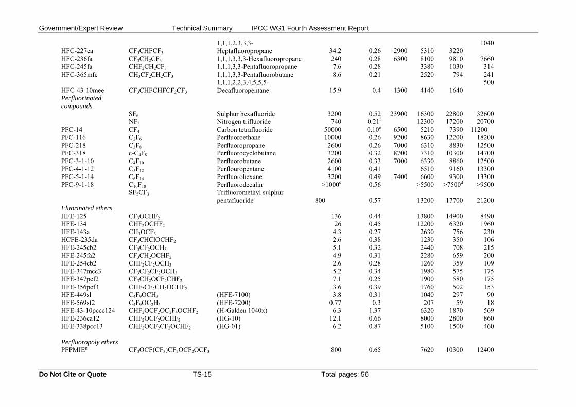
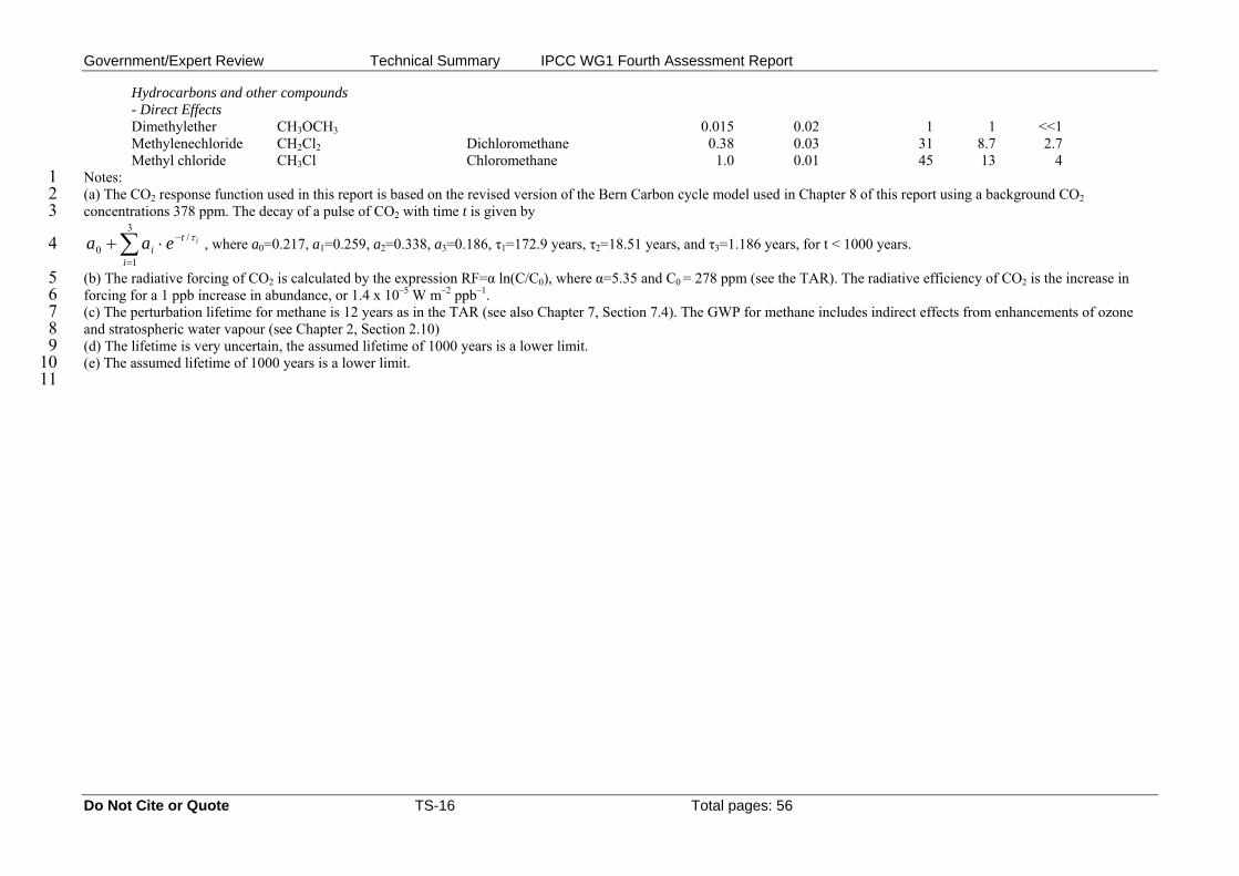
Table TS-2. (GWP Table, Table 2.14) Lifetimes, radiative efficiencies, and direct (except for methane) global warming potentials (GWP) relative to CO2. For ozone depleting substances and their replacements. Data are taken from IPCC/TEAP (2005) unless otherwise indicated.
Global Warming Potential for Given Time Horizon (years)
Industrial Designation or Common Name
Chemical Formula
Other Name
Lifetime (years)
Radiative Efficiency (W m-2 ppb-1) SAR
(100) 20 100 500Carbon dioxide CO2 See
belowa
b1.4x10-5 1 1 1 1
Methanec CH4 12c 3.7x10⁻⁴ 21 72 25 7.6 Nitrous oxide N2O 114c 3.03x10⁻³ 310 289 298 153 Substances controlled by the Montreal Protocol
CFC-11 CCl3F Trichlorofluoromethane 45 0.25 3800 6730 4750 1620CFC-12 CCl2F2 Dichlorodifluoromethane 100 0.32 8100 11000 10900 5200CFC-13 CClF3 Chlorotrifluoromethane 640 0.25 10800 14400 16400CFC-113 CCl2FCClF2 1,1,2-Trichlorotrifluoroethane 85 0.3 4800 6540 6130 2700CFC-114 CClF2CClF2 Dichlorotetrafluoroethane 300 0.31 8040 10000 8730CFC-115 CClF2CF3 Monochloropentafluoroethane 1700 0.18 5310 7370 9990Halon-1301 CBrF3 Bromotrifluoromethane 65 0.32 5400 8480 7140 2760Halon-1211 CBrClF2 Bromochlorodifluoromethane 16 0.3 4750 1890 575Halon-2402 CBrF2CBrF2 1,2-Dibromotettrafluoroethane 20 0.33 3680 1640 503Carbon tetrachloride CCl4 (Halon-104) 26 0.13 1400 2700 1400 435Methyl bromide CH3Br (Halon-1001) 0.7 0.01 17 5 1Methyl chloroform CH3CCl3 1,1,1-Trichloroethane 5 0.06 506 146 45HCFC-22 CHClF2 Chlorodifluoromethane 12 0.2 1500 5160 1810 549HCFC-123 CHCl2CF3 Dichlorotrifluoroethane 1.3 0.14 90 273 77 24HCFC-124 CHClFCF3 Chlorotetrafluoroethane 5.8 0.22 470 2070 609 185HCFC-141b CH3CCl2F Dichlorofluoroethane 9.3 0.14 2250 725 220HCFC-142b CH3CClF2 Chlorodifluoroethane 17.9 0.2 1800 5490 2310 705HCFC-225ca CHCl2CF2CF3 Dichloropentafluoropropane 1.9 0.2 429 122 37HCFC-225cb CHClFCF2CClF2 Dichloropentafluoropropane 5.8 0.32 2030 595 181Hydrofluorocarbons
HFC-23 CHF3 Trifluoromethane 270 0.19 11700 12000 14800 12200 HFC-32 CH2F2 Difluoromethane 4.9 0.11 650 2330 675 205 HFC-125 CHF2CF3 Pentafluoroethane 29 0.23 2800 6350 3500 1100 HFC-134a CH2FCF3 1,1,1,2-Tetrafluoroethane 14 0.16 1300 3830 1430 435 HFC-143a CH3CF3 1,1,1-Trifluoroethane 52 0.13 3800 5890 4470 1590 HFC-152a CH3CHF2 1,1-Difluoroethane 1.4 0.09 140 437 124 38
Do Not Cite or Quote TS-14 Total pages: 56
Government/Expert Review Technical Summary IPCC WG1 Fourth Assessment Report
HFC-227ea CF3CHFCF3
1,1,1,2,3,3,3-Heptafluoropropane 34.2 0.26 2900 5310 3220
1040
HFC-236fa CF3CH2CF3 1,1,1,3,3,3-Hexafluoropropane 240 0.28 6300 8100 9810 7660 HFC-245fa CHF2CH2CF3 1,1,1,3,3-Pentafluoropropane 7.6 0.28 3380 1030 314 HFC-365mfc CH3CF2CH2CF3 1,1,1,3,3-Pentafluorobutane 8.6 0.21 2520 794 241
HFC-43-10mee CF3CHFCHFCF2CF3
1,1,1,2,2,3,4,5,5,5-Decafluoropentane 15.9 0.4 1300 4140 1640
500
Perfluorinated compounds
SF6 Sulphur hexafluoride 3200 0.52 23900 16300 22800 32600 NF3 Nitrogen trifluoride 740 0.21f 12300 17200 20700 PFC-14 CF4 Carbon tetrafluoride 50000 0.10e 6500 5210 7390 11200 PFC-116 C2F6 Perfluoroethane 10000 0.26 9200 8630 12200 18200 PFC-218 C3F8 Perfluoropropane 2600 0.26 7000 6310 8830 12500 PFC-318 c-C4F8 Perfluorocyclobutane 3200 0.32 8700 7310 10300 14700 PFC-3-1-10 C4F10 Perfluorobutane 2600 0.33 7000 6330 8860 12500 PFC-4-1-12 C5F12 Perflouropentane 4100 0.41 6510 9160 13300 PFC-5-1-14 C6F14 Perfluorohexane 3200 0.49 7400 6600 9300 13300 PFC-9-1-18 C10F18 Perfluorodecalin >1000d 0.56 >5500 >7500d >9500
SF5CF3
Trifluoromethyl sulphur pentafluoride 800 0.57 13200 17700
21200
Fluorinated ethers HFE-125 CF3OCHF2 136 0.44 13800 14900 8490 HFE-134 CHF2OCHF2 26 0.45 12200 6320 1960 HFE-143a CH3OCF3 4.3 0.27 2630 756 230 HCFE-235da CF3CHClOCHF2 2.6 0.38 1230 350 106 HFE-245cb2 CF3CF2OCH3 5.1 0.32 2440 708 215 HFE-245fa2 CF3CH2OCHF2 4.9 0.31 2280 659 200 HFE-254cb2 CHF2CF2OCH3 2.6 0.28 1260 359 109 HFE-347mcc3 CF3CF2CF2OCH3 5.2 0.34 1980 575 175 HFE-347pcf2 CF3CH2OCF2CHF2 7.1 0.25 1900 580 175 HFE-356pcf3 CHF2CF2CH2OCHF2 3.6 0.39 1760 502 153 HFE-449sl C4F9OCH3 (HFE-7100) 3.8 0.31 1040 297 90HFE-569sf2 C4F9OC2H5 (HFE-7200) 0.77 0.3 207 59 18HFE-43-10pccc124 CHF2OCF2OC2F4OCHF2 (H-Galden 1040x) 6.3 1.37 6320 1870 569HFE-236ca12 CHF2OCF2OCHF2 (HG-10) 12.1 0.66 8000 2800 860HFE-338pcc13 CHF2OCF2CF2OCHF2 (HG-01) 6.2 0.87 5100 1500 460 Perfluoropoly ethers PFPMIEg CF3OCF(CF3)CF2OCF2OCF3 800 0.65 7620 10300 12400
Do Not Cite or Quote TS-15 Total pages: 56
Hydrocarbons and other compounds - Direct Effects
Dimethylether CH3OCH3 0.015 0.02 1 1 <<1Methylenechloride CH2Cl2 Dichloromethane 0.38 0.03 31 8.7 2.7Methyl chloride CH3Cl Chloromethane 1.0 0.01 45 13 4
ment/Expert Review Technical Summary IPCC WG1 Fourth Assessment Report
Do Not Cite or Quote TS-16 Total pages: 56
Notes: 1 2 3
4
5 6 7 8 9
10 11
(a) The CO2 response function used in this report is based on the revised version of the Bern Carbon cycle model used in Chapter 8 of this report using a background CO2 concentrations 378 ppm. The decay of a pulse of CO2 with time t is given by
∑=
−⋅+3
1
/0
i
ti
ieaa τ , where a0=0.217, a1=0.259, a2=0.338, a3=0.186, τ1=172.9 years, τ2=18.51 years, and τ3=1.186 years, for t < 1000 years.
(b) The radiative forcing of CO2 is calculated by the expression RF=α ln(C/C0), where α=5.35 and C0 = 278 ppm (see the TAR). The radiative efficiency of CO2 is the increase in forcing for a 1 ppb increase in abundance, or 1.4 x 10⁻⁵ W m–2 ppb–1. (c) The perturbation lifetime for methane is 12 years as in the TAR (see also Chapter 7, Section 7.4). The GWP for methane includes indirect effects from enhancements of ozone and stratospheric water vapour (see Chapter 2, Section 2.10) (d) The lifetime is very uncertain, the assumed lifetime of 1000 years is a lower limit. (e) The assumed lifetime of 1000 years is a lower limit.
Govern

Government/Expert Review Technical Summary IPCC WG1 Fourth Assessment Report
TS.3 OBSERVATIONS OF CHANGES IN CLIMATE 1 2 3 4 5 6 7 8 9
10 11 12 13 14 15 16 17 18 19 20 21 22 23 24 25 26 27 28 29 30 31 32 33 34 35 36 37 38 39 40 41 42 43 44 45 46 47 48 49 50 51 52 53 54 55 56
This assessment evaluates changes in the Earth’s climate system, considering not only the atmosphere, but also the ocean, and the cryosphere, as well as phenomena such as atmospheric circulation changes, in order to increase understanding of trends, variability, and processes of climate change at global and regional scales. Observational records employing direct methods are of variable length as described below, with global temperature estimates now beginning as early as 1850. Observations of extremes of weather and climate are discussed, and observed changes in extremes are described. The consistency of observed changes among different climate variables that allows an increasingly comprehensive picture to be drawn is also described. Finally, paleoclimatic information that generally employs indirect proxies to infer information about climate change on longer timescales up to millions of years is also assessed. TS.3.1 ATMOSPHERIC CHANGES: INSTRUMENTAL RECORD This assessment includes analysis of global and hemispheric means, changes over land and ocean, and distributions of trends in latitude, longitude, and altitude. Since the TAR, improvements in observations and their calibration, more detailed analysis of methods, and extended time series allow more in-depth analyses of changes including atmospheric temperature, precipitation, humidity, wind, and circulation. Extremes of climate are a key expression of climate variability, and this assessment also includes new data that permit improved insights into the changes in many types of extreme events including heat waves, droughts, heavy precipitation, and tropical cyclones (including hurricanes and typhoons). {3.2, 3.3, 3.4, 3.8} Furthermore, advances have occurred since the TAR in understanding how a number of seasonal and long-term anomalies can be described by patterns of climate variability. These patterns arise from internal interactions and from the differential effects on the atmosphere of land and ocean, mountains, and large changes in heating. Their response is often felt in regions far removed from their physical source through atmospheric teleconnections associated with large-scale waves in the atmosphere. Understanding temperature and precipitation anomalies associated with the dominant patterns of climate variability is essential to understanding many regional climate anomalies and why these may differ from those at the global scale. Changes in storm tracks, the jet streams, regions of preferred blocking anticyclones, and changes in monsoons can also occur in conjunction with these preferred patterns of variability. {3.5, 3.6, 3.7} TS.3.1.1 Globally Averaged Temperatures 2005 and 1998 were the warmest two years in the instrumental global air surface temperature record since 1850. Surface temperatures in 1998 were enhanced by the major 1997–1998 El Niño but no such strong anomaly was present in 2005. Eleven of the last twelve years (1995 to 2006) – the exception being 1996 – rank among the 12 warmest years on record since 1850. (Preliminary result for 2006 to be checked before the final WG1 plenary in 2007.) {3.2}
The global average surface temperature has increased, especially since about 1950. The updated 100-year trend (1906–2005) of 0.74 ± 0.18°C is larger than the 100-year warming trend at the time of the TAR (1901–2000) of 0.6 ± 0.2°C due to additional warm years. The rate of warming averaged over the last 50 years (0.13 ± 0.03°C per decade) is nearly twice that for the last 100 years. Three different global estimates all show consistent warming trends. There is also consistency between the datasets in their separate land and ocean domains, and between sea surface temperature (SST) and night-time marine air temperature. (See Figure TS-6) {3.2} [INSERT FIGURE TS-6 HERE] Recent studies confirm that effects of urbanization and land use change on the global temperature record (since 1950) are negligible as far as hemispheric- and continental-scale averages are concerned. All observations are subject to data quality and consistency checks to correct for potential biases. The real but local effects of urban areas are accounted for in the land temperature datasets used. Urbanization and land-use effects are not relevant to the widespread oceanic warming that has been observed. Increasing evidence
Do Not Cite or Quote TS-17 Total pages: 56
Government/Expert Review Technical Summary IPCC WG1 Fourth Assessment Report
1 2 3 4 5 6 7 8 9
10 11 12 13 14 15 16 17 18 19 20 21 22 23 24 25 26 27 28 29 30 31 32 33 34 35 36 37 38 39 40 41 42 43 44 45 46 47 48 49 50 51 52 53 54 55 56 57
suggests that urban heat island effects also affect precipitation, cloud, and diurnal temperature range (DTR). {3.2} The global average diurnal temperature range has stopped decreasing. The averaged DTR over land decreased by about 0.07ºC per decade from 1950 to 1980 but has since levelled off. {3.2} New analyses of radiosonde and satellite measurements of lower- and mid-tropospheric temperature show warming rates that are generally consistent with each other and with those in the surface temperature record within their respective uncertainties for the periods 1958–2005 and 1979 –2005. This largely resolves a discrepancy noted in the TAR (see Figure TS-7). The radiosonde record is markedly less spatially complete than the surface record and increasing evidence suggests a number of radiosonde datasets are unreliable, especially in the tropics. Disparities remain among different tropospheric temperature trends estimated from satellite microwave sounder unit (MSU) and advanced MSU (AMSU) measurements since 1979, and all likely still contain residual errors. However, trend estimates have been substantially improved and dataset differences reduced since the TAR through adjustments for changing satellites, orbit decay, and drift in local crossing time (diurnal cycle effects). It appears that the satellite tropospheric temperature record is broadly consistent with surface temperature trends provided that the stratospheric influence on MSU channel 2 is accounted for. The range across different datasets of global surface warming since 1979 is 0.16 to 0.18, compared to 0.12 to 0.19ºC per decade for MSU-derived estimates of tropospheric temperatures. It is likely that there is increased warming with altitude from the surface through much of the troposphere in the tropics, pronounced cooling in the stratosphere, and a trend towards a higher tropopause. {3.4} [INSERT FIGURE TS-7 HERE] Stratospheric temperature estimates from adjusted radiosondes, satellites, and reanalyses are all in qualitative agreement, with a cooling of between 0.3 and 0.6°C per decade since 1979 (see Figure TS-7). Longer radiosonde records (back to 1958) also indicate stratospheric cooling but are subject to substantial instrumental uncertainties. The rate of cooling increased after 1979 but has slowed in the last decade. It is likely that radiosonde records overestimate stratospheric cooling, owing to changes in sondes not yet taken into account. The trends are not monotonic, because of stratospheric warming episodes that follow major volcanic eruptions. {3.4} TS.3.1.2 Spatial Distribution of Changes in Temperature, Circulation and Related Variables Surface temperatures over land regions have warmed at a faster rate than over the oceans in both hemispheres. Longer records now available show significantly faster rates of warming over land than ocean in the past two decades (about 0.27 versus 0.13°C per decade). {3.2} The warming in the last 30 years is widespread over the globe, and is a maximum at higher northern latitudes. The greatest warming has occurred in the Northern Hemisphere winter (DJF) and spring (MAM). Average Arctic temperatures have been increasing at almost twice the rate of the rest of the world in the past 100 years. However, Arctic temperatures are highly variable. A slightly longer warm period, almost as warm as the present, was observed from 1925–1945, but its geographical extent appears to have been different from the recent warming. {3.2} There is evidence for long-term changes in the large-scale atmospheric circulation, such as a poleward shift and strengthening of the westerly winds. Regional climate trends can be very different from the global average, reflecting changes in the circulations and interactions of the atmosphere and ocean and the other components of the climate system. Stronger mid-latitude westerly wind maxima have occurred in both hemispheres in most seasons from at least 1979 to the late 1990s, and poleward displacements of corresponding Atlantic and southern polar front jet streams have been documented. The westerlies in the Northern Hemisphere increased from the 1960s to the 1990s but have since returned to values close to the long-term average. The increased strength of the westerlies in the Northern Hemisphere changes the flow from oceans to continents, and is a major factor in the observed wintertime changes in storm tracks and related patterns of precipitation and temperature trends at mid- and high-latitudes. Analyses of wind and significant wave height support reanalysis-based evidence for changes in extratropical storms in the Northern Hemisphere from the start of the reanalysis record in the late 1970s until the late 1990s. These changes are
Do Not Cite or Quote TS-18 Total pages: 56
Government/Expert Review Technical Summary IPCC WG1 Fourth Assessment Report
1 2 3 4 5 6 7 8 9
10 11 12 13 14 15 16 17 18 19 20 21 22 23 24 25
accompanied by a tendency toward stronger wintertime polar vortices throughout the troposphere and lower stratosphere. {3.2, 3.5} Many regional climate changes can be described in terms of preferred patterns of climate variability and therefore as changes in the occurrence of values of the indices of these. The importance on all time-scales of fluctuations in the westerlies and the storm-track in the North Atlantic have often been noted and described by the NAO (see Box TS.3.1 for an explanation of this and other preferred patterns). The characteristics of fluctuations in the zonally averaged westerlies in the two hemispheres has more recently been described by their respective “ annular modes”, the Northern and Southern Annular Modes (NAM and SAM). The observed changes can be expressed as a shift of the circulation towards the structure associated with one sign of these preferred patterns. The increased middle latitude westerlies in the North Atlantic can be largely viewed as reflecting either NAO or NAM changes; multi-decadal variability is also evident in the Atlantic, both in the atmosphere and the ocean. In the Southern Hemisphere, changes in circulation related to an increase in the SAM from the 1960s to the present are associated with strong warming over the Antarctic Peninsula and, to a lesser extent, cooling over parts of continental Antarctica. Changes have also been observed in ocean-atmosphere interactions in the Pacific. ENSO is the dominant mode of global-scale variability on interannual time scales although there have been times when it is less apparent. The 1976–1977 climate shift, related to the phase change in the Pacific Decadal Oscillation (PDO) toward more El Niño events and changes in the evolution of ENSO, has affected many areas, including most tropical monsoons. For instance, over North America, ENSO and PNA teleconnection-related changes appear to have led to contrasting changes across the continent, as the West has warmed more than the East, while the latter has become cloudier and wetter. There is substantial low-frequency atmospheric variability in the Pacific sector over the 20th century, with extended periods of weakened (1900–1924; 1947–1976) as well as strengthened circulation (1925–1946; 1977–2003). {3.2, 3.5, 3.6}
26 BOX TS.3.1: PATTERNS (MODES) OF CLIMATE VARIABILITY 27
Analysis of atmospheric/climate variability has shown that a significant component of it can be described in 28 terms of fluctuations in the amplitude and sign of indices of a relatively small number of preferred patterns 29 of variability. Some of the best known of these are: 30
31 • El Niño-Southern Oscillation (ENSO), a coupled fluctuation in the atmosphere and the equatorial Pacific 32
Ocean, with preferred times scales of 2 to about 7 years. ENSO is often measured by the surface pressure 33 anomaly difference between Tahiti and Darwin and the sea surface temperatures in the central and 34 eastern equatorial Pacific. ENSO has global teleconnections. 35
• North Atlantic Oscillation (NAO), a measure of the strength of the Icelandic Low and the Azores high, 36 and also of the westerly winds between them, mainly in winter. The NAO has associated fluctuations in 37 the storm-track, temperature and precipitation from the North Atlantic into Eurasia. (See Box TS.3.1, 38 Figure 1) 39
• Northern Annular Mode (NAM), a winter-time fluctuation in the amplitude of a pattern characterised by 40 low surface pressure in the Arctic and strong middle latitude westerlies. The NAM has links with the 41 northern polar vortex into the stratosphere. Its pattern has a bias to the North Atlantic and it has a high 42 correlation with the NAO. 43
• Southern Annular Mode (SAM), the fluctuation of a pattern with low Antarctic surface pressure and 44 strong mid-latitude westerlies, analogous to the NAM, but present year-round. 45
• Pacific North American (PNA) pattern, an atmospheric large-scale wave pattern featuring a sequence of 46 tropospheric high and low pressure anomalies stretching from the subtropical west Pacific to the east 47 coast of North America. 48
• Pacific Decadal Oscillation (PDO), a measure of the sea surface temperatures in the North Pacific that 49 has a very strong correlation with the North Pacific Index (NPI) measure of the depth of the Aleutian 50 Low. However, it has a signature throughout much of the Pacific. 51
52 53 [INSERT FIGURE BOX TS.3.1, FIGURE 1 HERE] 54
The extent to which all these preferred patterns of variability can be considered to be true modes of the 55 climate system is a topic of active research. However there is evidence that their existence can lead to larger 56 amplitude regional responses to forcing than would otherwise be expected. In particular, a number of the 57 Do Not Cite or Quote TS-19 Total pages: 56

Government/Expert Review Technical Summary IPCC WG1 Fourth Assessment Report
observed 20th century climate changes can be viewed in terms of changes in them. It is therefore important 1 to test the ability of climate models to simulate them (see Box TS.4.1) and to consider the extent to which 2 observed changes related to these patterns are linked to internal variability or to anthropogenic climate 3 change. {3.6, 8.4} 4
5 6 7 8 9
10 11 12 13 14 15 16 17 18 19 20 21 22 23 24 25 26 27 28 29 30 31 32 33 34 35 36 37 38 39 40 41 42 43 44 45 46 47 48 49 50 51 52 53 54 55 56 57
Changes in extremes of temperature are consistent with warming. Widespread reductions have been observed in the number of frost days in mid-latitude regions, increases in the number of warm extremes (warmest 10% of days or nights) and a reduction in the number of daily cold extremes (coldest 10% of days or nights) (see Box TS.3.4). The most marked changes are for cold nights, which have declined over the 1951–2003 period for all regions where data are available (76% of the land). {3.8} Heat waves have increased in duration beginning in the latter half of the 20th century. The record-breaking heat wave over western and central Europe in the summer of 2003 is an example of an exceptional recent extreme. That summer (JJA) was the warmest since comparable instrumental records began around 1780 (1.4ºC above the previous warmest in 1807). Spring drying of the land surface over Europe was an important factor in the occurrence of the extreme 2003 temperatures. Evidence suggests that heat waves have also increased in frequency and duration in other locations. The very strong correlation between observed dryness and high temperatures over land in the summer and the tropics highlights the important role moisture plays in moderating climate. {3.8} There is insufficient evidence to determine whether trends exist in, for example, tornadoes, hail, lightning and dust-storms on small scales. {3.8} TS.3.1.3 Changes in the Water Cycle: Water Vapour, Clouds, Precipitation, and Tropical Storms Tropospheric water vapor is increasing (Figure TS-8). Surface specific humidity has generally increased after 1976 in close association with higher temperatures over both land and ocean. Total column water vapour has increased over the global oceans by 1.2 ± 0.3% per decade (95% confidence limits) from 1988–2004. The observed regional changes are consistent in pattern and amount with the changes in SST and the assumption of a near-constant relative humidity increase in water vapour mixing ratio. The additional atmospheric water vapour implies increased moisture availability for precipitation. {3.4} Upper-tropospheric water vapour is also increasing. Due to instrumental limitations, there is difficulty in assessing long-term changes in water vapour in the upper troposphere, where it is of radiative importance. However the available data now show evidence for global increases in upper tropospheric specific humidity over the past two decades (Figure TS-8). These observations are consistent with the observed increase in temperatures and represent an important advance since the TAR. {3.4} [INSERT FIGURE TS-8 HERE] Cloud changes are dominated by ENSO. Widespread (but not ubiquitous) decreases in continental DTR have coincided with increases in cloud amounts. Total and low-level cloud changes over the ocean disagree between surface and satellite observations. However, radiation changes at the top-of-the atmosphere from the 1980s to 1990s (possibly related in part to the El Niño Southern Oscillation (ENSO) phenomenon), appear to be associated with reductions in tropical upper-level cloud cover, and are consistent with changes in the energy budget and in observed ocean heat content. {3.4} “Global dimming” is not global in extent and it has not continued after 1990. Reported decreases in solar radiation at the Earth’s surface from 1970 to 1990 have an urban bias. Further, there have been increases since about 1990. An increasing aerosol load due to human activities decreases regional air quality and the amount of solar radiation reaching the earth’s surface. In some areas, such as Eastern Europe, recent observations of a reversal in sign of this effect link changes in solar radiation to concurrent air quality improvements. {3.4} Long-term trends from 1900 to 2005 have been observed in precipitation amount in many large regions (Figure TS-9). Significantly increased precipitation is observed in eastern parts of North and South America, northern Europe and northern and central Asia. Drying has been observed in the Sahel, the Mediterranean,
Do Not Cite or Quote TS-20 Total pages: 56

Government/Expert Review Technical Summary IPCC WG1 Fourth Assessment Report
southern Africa and parts of southern Asia. Precipitation is highly variable spatially and temporally, androbust long term trends have not been established for other large regions. {3.3}
1 2 3 4 5 6 7 8 9
10 11 12 13 14 15 16 17 18 19 20 21 22 23 24 25 26 27 28 29 30 31 32 33 34 35 36 37 38 39 40 41 42 43 44 45 46 47 48 49 50 51 52
[INSERT FIGURE TS-9 HERE] Substantial increases have been observed in heavy precipitation events. It is likely that there have been increases in the number of heavy precipitation events (e.g., above the 95th percentile) in many land regions since about 1950, even those where there has been a reduction in total precipitation amount. Increases have also been reported for rarer precipitation events (1 in 50 year return period), but only a few regions have sufficient data to assess such trends reliably (see Figure TS-10). {3.8} [INSERT FIGURE TS-10 HERE] There is evidence that the number and proportion of tropical cyclones reaching the most intense categories has increased since 1970, although there is no clear trend in the total numbers of tropical cyclones. Estimates of the potential destructiveness of tropical cyclones suggest a substantial upward trend since the mid-1970s, with a trend towards longer lifetimes and greater intensity. Trends are also apparent in SST, a critical variable known to influence tropical cyclone development (see Figure TS-11). Data quality and coverage issues, particularly prior to the satellite era, are obstacles to analysis of variations in tropical cyclones on longer time scales. Variations in the total numbers of tropical cyclones result from ENSO and decadal variability, which also lead to a redistribution of tropical storm numbers and tracks. The numbers of hurricanes in the North Atlantic have been above normal (based on 1981 – 2000) in 9 of the years from 1995 to 2005. {3.8} [INSERT FIGURE TS-11 HERE] More intense and longer droughts have been observed over wider areas, particularly in the tropics and subtropics since the 1970s. While there are many different measures of drought, many studies use precipitation changes together with temperature5. Increased drying due to higher temperatures and decreased land precipitation have contributed to these changes. {3.3} TS.3.2 CHANGES IN THE CRYOSPHERE: INSTRUMENTAL RECORD Currently ice permanently covers 10% of the land surface, with only a tiny fraction occurring outside Antarctica and Greenland. Ice also covers approximately 7% of the oceans in the annual mean. In mid-winter, snow covers approximately 49% of the land surface in the Northern Hemisphere. An important property of snow and ice is its high surface albedo. Because up to 90% of the incident solar radiation is reflected by snow and ice surfaces, while only about 10% is reflected by the open ocean or forested lands, changes in snow and ice cover are important feedback mechanisms in climate change. In addition, snow and ice are effective insulators. Seasonally frozen ground is more extensive than snow cover, and its presence is also important for energy and moisture fluxes. Therefore, frozen surfaces play important roles in energy and climate processes. {4.1} The cryosphere stores about 75% of the world’s fresh water. On a regional scale, variations in mountain snowpack, glaciers and small ice caps play a crucial role in fresh water availability. Since the change from ice to liquid water occurs at specific temperatures, ice is a component of the climate system that could be subject to abrupt change following sufficient warming. Observations and analyses of changes in ice have expanded and improved since the TAR, including shrinkage of mountain glacier volume, decreases in snow cover, changes in permafrost and frozen ground, reductions in Arctic sea ice extent, coastal thinning of the Greenland ice sheet exceeding inland thickening from increased snowfall, and reductions in seasonally frozen ground, river and lake ice cover. These allow an improved understanding of how the cryosphere is changing, including its contributions to recent changes in sea level. The periods from 1961-present and
5 Precipitation and temperature are combined in the Palmer Drought Severity Index (PDSI) considered in this report as one measure of drought. PDSI does not include variables such as wind speed, solar radiation, cloudiness, and water vapour but is a superior measure to precipitation alone. Do Not Cite or Quote TS-21 Total pages: 56

Government/Expert Review Technical Summary IPCC WG1 Fourth Assessment Report
1 2 3 4 5 6 7 8 9
10 11 12 13 14 15 16 17 18 19 20 21 22 23 24 25 26 27 28 29 30 31 32 33 34 35 36 37 38 39 40 41 42 43 44 45 46 47 48 49 50 51 52 53 54 55 56
1993-present are a focus of this report, due to the availability of directly measured glacier mass balance data and altimetry observations of the ice sheets, respectively. {4.1} Snow cover has decreased in most regions, especially in spring. Northern Hemisphere snow cover observed by satellite over the 1966–2005 period decreased in every month except November and December, with a stepwise drop of 5% in the annual mean in the late 1980s (see Figure TS-12). In the Southern Hemisphere, the few long records or proxies mostly show either decreases or no changes in the past 40+ years. Northern Hemisphere April snow cover extent is strongly correlated with 40–60°N April temperature, reflecting the feedback between snow and temperature. {4.2} [INSERT FIGURE TS-12 HERE] Decreases in snowpack have been documented in several regions worldwide based upon annual time series of mountain snow water equivalent and snow depth. Mountain snow can be sensitive to small changes in temperature, particularly in temperate climatic zones where the transition from rain to snow is generally closely associated with the altitude of the freezing level. Declines in mountain snows in western North America and in the Swiss Alps are largest at lower, warmer elevations. Mountain snow water equivalent has declined since 1950 at 75% of the stations monitored in western North America. Mountain snow depth has also declined in the Alps and in southeastern Australia. Direct observations of snow depth are too limited to determine changes in the Andes, but temperature measurements suggest that the altitude where snow occurs (above the snowline) has probably risen in mountainous regions of South America. {4.2} Permafrost and seasonally frozen ground in most regions display large changes in recent decades. Changes in permafrost conditions can affect river runoff, water supply, carbon exchange, and landscape stability, and can cause damage to infrastructure. Temperature increases at the top of the permafrost layer by up to 3°C since the 1980s have been reported. Permafrost warming is also observed with variable magnitude in the Canadian Arctic, Siberia, Tibetan Plateau, and Europe. The permafrost base is thawing at a rate ranging from 0.04 m yr-1 in Alaska to 0.02 m yr-1 on the Tibetan Plateau. {4.7} The maximum area covered by seasonally frozen ground decreased by about 7% in the Northern Hemisphere over the latter half of the 20th century. Its maximum depth has decreased by about 0.3 m in Eurasia since the mid-20th century. In addition, maximum seasonal thaw depth has increased about 0.2 m in the Russian Arctic from 1956 to 1990. {4.7} On average, the general trend of Northern Hemisphere river and lake ice over the past 150 years indicates that the freeze-up date has become later at an average rate of 5.8 ± 1.9 days per century, while the break-up date has occurred earlier, at a rate of 6.5 ± 1.4 days per century. However, considerable spatial variability is also observed, with some regions showing trends of opposite sign. {4.3} Annually averaged Arctic sea ice extent has shrunk by about 2.7% ± 0.7% per decade since 1978 based upon satellite observations (see Figure TS-13). The decline for summertime extent is larger than for wintertime, with the summer minimum declining at a rate of about 7.4% ± 2.9% per decade. Other data indicate that the summer decline began around 1970. Similar observations in the Antarctic reveal larger inter-annual variability but no consistent trends during the period of satellite observations. In contrast to changes in continental ice such as ice sheets and glaciers, changes in sea ice do not directly contribute to sea level change (because this ice is already floating), but can contribute to salinity changes through input of freshwater. {4.4} [INSERT FIGURE TS-13 HERE] During the 20th century, glaciers and ice caps have experienced widespread mass losses and have contributed to sea level rise. Mass loss of glaciers and ice caps (excluding those around the ice sheets of Greenland and Antarctica), is estimated to be 0.50 ± 0.18 mm in sea level equivalent (SLE) per year between 1961 and 2003, and 0.77 ± 0.22 mm SLE per year between 1991 and 2003. The late 20th century glacier wastage likely has been a response to post-1970 warming. {4.5}
Do Not Cite or Quote TS-22 Total pages: 56

Government/Expert Review Technical Summary IPCC WG1 Fourth Assessment Report
1 2 3 4 5 6 7 8 9
10 11 12 13 14 15 16 17 18 19 20 21 22 23 24 25 26 27 28 29 30 31 32
Recent observations show evidence for rapid changes in ice flow in some regions, contributing to sea level rise and suggesting that the dynamics of ice motion may be a key factor in future responses of ice shelves, coastal glaciers, and ice sheets to climate change. Thinning or loss of ice shelves in some near-coastal regions of Greenland and the Antarctic Peninsula, and West Antarctica has been associated with accelerated flow of nearby glaciers and ice streams, suggesting that ice shelves (including short ice shelves of kilometers or tens of kilometers) could play a larger role in stabilizing or restraining ice motion than previously thought. Both oceanic and atmospheric temperatures appear to contribute to the observed changes. Large summer warming in the Antarctic Peninsula region very likely played a role in the subsequent rapid breakup of the Larsen B ice shelf in 2002 by increasing summer meltwater, which drained into crevasses and wedged them open. Models do not accurately capture all of the physical processes that appear to be involved in observed iceberg calving (as in the breakup of Larsen B). {4.6} The Greenland and Antarctic ice sheets are very likely contributing to the sea level rise of the past decade. Greenland is very likely to have shrunk from 1993–2003, with thickening in central regions more than offset by increased melting in coastal regions. Whether the ice sheets have been growing or shrinking over timescales of longer than a decade is not well established from observations. Lack of agreement between techniques and the small number of estimates, preclude assignment of best estimates or statistically rigorous error bounds for changes in ice sheet mass balances. However, acceleration of outlet glaciers drains ice from the interior and has been observed in both ice sheets (see Figure TS-14). Assessment of the data and techniques suggests a mass balance of the Greenland Ice Sheet of –50 to –100 Gt per year (shrinkage contributing to raising global sea level by 0.14 to 0.28 mm yr–1) during 1993–2003, with even larger losses in 2005. There are greater uncertainties for earlier time periods and for Antarctica. The estimated range in mass balance for the Greenland ice sheet over 1961–2003 is between growth of 25 and shrinkage by 60 Gt yr-1 (–0.07 to 0.17 mm yr–1 SLE). Assessment of all the data yields an estimate for the overall Antarctic ice-sheet mass balance ranging from growth of 100 Gt to shrinkage of 200 Gt per year (–0.28 to +0.55 mm yr–1 SLE) 1 from 1961 to 2003, and from +50 Gt to –200 Gt per year (–0.14 to +0.55 mm yr–1 SLE) from 1993–2003. The recent changes in ice-flow are likely to be sufficient to explain much or all of the restimated Antarctic mass imbalance, with recent changes in ice-flow, snowfall and meltwater runoff sufficient to explain the mass imbalance of Greenland. {4.6, 4.8} [INSERT FIGURE TS-14 HERE]
33 BOX TS.3.2: ICE SHEET DYNAMICS AND STABILITY34
Ice sheets are thick, broad masses of ice formed mainly from compaction of snow. They spread under their 35 own weight, transferring mass towards their margins where it is lost primarily by runoff of surface meltwater 36 or by calving of icebergs into marginal seas or lakes. Ice sheets flow by deformation within the ice or 37 meltwater-lubricated sliding over materials beneath. Rapid basal motion requires that the basal temperature 38 be raised to the melting point by heat from the earth’s interior, delivered by meltwater transport, or from the 39 “friction” of ice motion. Sliding velocities under a given gravitational stress can differ by several orders of 40 magnitude, depending on the presence or absence of deformable sediment, the roughness of the substrate, 41 and the supply and distribution of water. Basal conditions are generally poorly characterized, introducing 42 important uncertainties to the understanding of ice sheet stability. {4.6} 43
44 Ice flow is often channeled into fast-moving ice streams (which flow between slower-moving ice walls) or 45 outlet glaciers (with rock walls). Enhanced flow in ice streams arises either from higher gravitational stress 46 linked to thicker ice in bedrock troughs, or from increased basal lubrication. 47
48 {4.6} 49
Ice discharged across the coast often remains attached to the ice sheet to become a floating ice shelf. An ice 50 shelf moves forward, spreading and thinning under its own weight, and fed by snowfall on its surface and ice 51 input from the ice sheet. Friction at ice-shelf sides and over local shoals slows the flow of the ice shelf and 52 thus the discharge from the ice sheet. An ice shelf loses mass by calving icebergs from the front and by basal 53 melting into the ocean cavity beneath. Studies suggest a 1°C ocean warming could increase ice-shelf basal 54 melt by 10 m per year, but inadequate knowledge of the largely inaccessible ice shelf cavities restricts the 55 accuracy of such estimates. {4.6} 56
57
Do Not Cite or Quote TS-23 Total pages: 56

Government/Expert Review Technical Summary IPCC WG1 Fourth Assessment Report
The paleo-record of previous ice ages indicates that ice sheets shrink in response to warming and grow in 1 response to cooling, and that shrinkage can be far faster than growth. The volumes of the Greenland and 2 Antarctic ice sheets are equivalent to approximately 7 m and 57 m of sea level rise, respectively. 3 Paleoclimatic data indicate that substantial melting of one or both ice sheets has likely occurred in the past. 4 However, ice core data show that neither ice sheet was completely removed during warm periods of at least 5 the past million years. Ice-sheets can respond to environmental forcing on very slow time scales, implying 6 that commitments to future changes may result from current warming. For example, a surface warming may 7 take more than 10,000 years to penetrate to the bed and change temperatures there. Ice velocity over most of 8 an ice sheet changes slowly in response to changes in the ice sheet shape or surface temperature, but large 9 velocity changes may occur rapidly on ice streams and outlet glaciers in response to changing basal 10 conditions, penetration of surface meltwater to the bed, or changes in the ice shelves into which they flow. 11 {4.6, 6.4} 12
13 Models currently configured for long integrations remain most reliable in their treatment of surface 14 accumulation and ablation, as for the TAR, but do not include full treatments of ice dynamics; thus, analyses 15 of past changes or future projections using such models may underestimate ice-flow contributions to sea 16 level rise, but the magnitude of such an effect is unknown. {8.2} 17
18 19 20 21 22 23 24 25 26 27 28 29 30 31 32 33 34 35 36 37 38 39 40 41 42 43 44 45 46 47 48 49 50 51 52 53 54 55 56 57
TS.3.3 CHANGES IN THE OCEAN: INSTRUMENTAL RECORD The ocean plays an important role in climate and climate change. The ocean is influenced by mass, energy and momentum exchanges with the atmosphere. Its heat capacity is about 1000 times larger than that of the atmosphere and the ocean's net heat uptake is therefore many times greater than that of the atmosphere (see Figure TS-15). Global observations of the heat taken up by the ocean can now be shown to be a definitive test of changes in the global energy budget. Changes in the amount of energy taken up by the upper layers of the ocean also play a crucial role for climate variations on seasonal to inter-annual time scales, such as El Niño. Changes in the transport of heat and sea-surface temperatures have important effects upon many regional climates worldwide. Life in the sea is dependent on the biogeochemical status of the ocean and is affected by changes in the physical state and circulation. Changes in ocean biogeochemistry can also feed back into the climate system, e.g., through changes in uptake or release of radiatively active gases such as CO2. {5.1, 7.3} [INSERT FIGURE TS-15 HERE] Global mean sea level variations are driven in part by changes in density, through thermal expansion or contraction of the ocean’s volume. Local changes in sea level also have a density-related component due to temperature and salinity changes. In addition, exchange of water between oceans and other reservoirs (e.g., ice sheets, mountain glaciers, land water reservoirs and atmosphere) can change the ocean’s mass and hence contribute to changes in sea level. Sea level change is not geographically uniform because processes such as ocean circulation changes are not uniform across the globe (see Box TS.3.3). {5.5} Oceanic variables can be useful for climate change detection, in particular temperature and salinity changes below the surface mixed layer where the variability is smaller and signal-to-noise ratio is higher. Observations analysed since the TAR have provided new evidence for changes in global ocean heat content and salinity, sea level, thermal expansion contributions to sea level rise, water mass evolution and bio-geochemical cycles. {5.5} TS.3.3.1 Changes in Ocean Heat Content and Circulation The world ocean has warmed since 1955, accounting over this period for about 90% of the changes in the energy content of the Earth’s climate system. A total of 7.9 million vertical profiles of ocean temperature allows construction of improved global time series (see Figure TS-16). Analyses of the global oceanic heat budget have been replicated by several independent analysts and are robust to the method used. Data coverage limitations require averaging over decades for the deep ocean and observed decadal variability in the global heat content is not fully understood. However, inadequacies in the distribution of data (particularly coverage in the Southern Ocean and South Pacific) could contribute to the apparent decadal variations in heat content. During the period 1961–2003 the 0–3000 m ocean layer has taken up about 14.1 x 10²² J,
Do Not Cite or Quote TS-24 Total pages: 56

Government/Expert Review Technical Summary IPCC WG1 Fourth Assessment Report
equivalent to an average heating rate of 0.2 W m–2 (per unit area of the Earth’s surface). During 1993–2003, the corresponding rate of warming in the shallower 0–700 m ocean layer was higher, about 0.5±0.18 W m
1 2 3 4 5 6 7 8 9
10 11 12 13 14 15 16 17 18 19 20 21 22 23 24 25 26 27 28 29 30 31 32 33 34 35 36 37 38 39 40 41 42 43 44 45 46 47 48 49 50 51 52 53 54
-2. Relative to 1961–2003, the period 1993–2003 had high rates of warming but in 2004 and 2005 there has been some cooling compared to 2003. {5.1, 5.2, 5.3} [INSERT FIGURE TS-16 HERE]
Warming is widespread over the upper 700 meters of the global ocean. The Atlantic has warmed south of 45°N. The warming is penetrating deeper in the Atlantic ocean basin than in the Pacific, Indian and Southern Oceans, due to the deep overturning circulation cell that occurs in the North Atlantic. The Southern Hemisphere deep overturning circulation shows little evidence of change based on available data. However, the upper layers of the Southern Ocean contribute strongly to the overall warming. At least two seas at subtropical latitudes (Mediterranean and Japan/East China Sea) are warming. While the global trend is one of warming, significant decadal variations are observed in the global time series, and there are large regions where the oceans are cooling. Parts of the North Atlantic, North Pacific and Equatorial Pacific have cooled over the last 50 years. The changes in the Pacific Ocean show ENSO-like spatial patterns linked in part to the Pacific Decadal Oscillation. {5.2, 5.3} Parts of the Atlantic meridional overturning circulation exhibit considerable decadal variability, but data do not support a coherent trend in the overturning circulation. {5.3} TS.3.3.2 Changes in Ocean Biogeochemistry and Salinity The uptake of anthropogenic carbon since 1750 has led to the ocean becoming more acidic, with an average decrease in surface pH by 0.1 units 6. Uptake of carbon dioxide by the ocean changes its chemical equilibrium. Dissolved CO2 forms a weak acid so, as dissolved CO2 increases, pH decreases; i.e., the ocean becomes more acidic. The overall pH change is computed from estimates of anthropogenic carbon uptake and simple ocean models. Direct observations of pH at available stations for the last 20 years also show trends of decreasing pH, at a rate of about 0.02 pH units per decade. Decreasing ocean pH decreases the depth below which calcium carbonate dissolves and increases the volume of the ocean that is undersaturated with respect to the minerals aragonite (a meta-stable form of calcium carbonate) and calcite, which are used by marine organisms to build their shells. Decreasing surface ocean pH and rising surface temperatures also act to reduce the ocean buffer capacity for CO2 and the rate at which the ocean can take up excess atmospheric CO2. {5.4, 7.3} The oxygen concentration of the ventilated thermocline (~100–1000 m) decreased in most ocean basins between 1970 and 1995. These changes may reflect a reduced rate of ventilation linked to upper level warming and/or changes in biological activity. {5.4} There is now widespread evidence for changes in ocean salinity on gyre and basin scales in the past half-century (see Figure TS-17) with the near surface waters in the more evaporative regions increasing in salinity in almost all ocean basins. These changes in salinity imply changes in the hydrological cycle over the oceans. In the high latitude regions in both hemispheres, the surface waters show an overall freshening consistent with these regions having greater precipitation, although higher run-off, ice melting, advection, and changes in the meridional overturning circulation may also contribute. The sub-tropical latitudes in both hemispheres in the upper 500 m are characterised by an increase in salinity. The patterns are consistent with a change in the earth's hydrological cycle, in particular with changes in precipitation and inferred larger water transport in the atmosphere from low latitudes to high latitudes and from the Atlantic to the Pacific. {52} [INSERT FIGURE TS-17 HERE] TS.3.3.3 Changes in Sea Level
6 Acidity is a measure of the concentration of H+ ions and is reported in pH units, where pH = –log(H+). A pH decrease of 1 unit means a 10-fold increase in the concentration of H+, or acidity. Do Not Cite or Quote TS-25 Total pages: 56
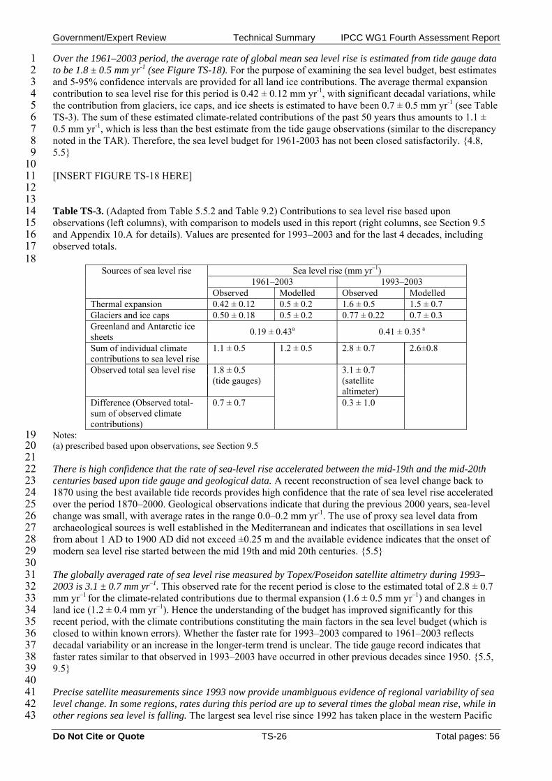
Government/Expert Review Technical Summary IPCC WG1 Fourth Assessment Report
Over the 1961–2003 period, the average rate of global mean sea level rise is estimated from tide gauge data to be 1.8 ± 0.5 mm yr
1 2 3 4 5 6 7 8 9
10 11 12 13 14 15 16 17 18
-1 (see Figure TS-18). For the purpose of examining the sea level budget, best estimates and 5-95% confidence intervals are provided for all land ice contributions. The average thermal expansion contribution to sea level rise for this period is 0.42 ± 0.12 mm yr-1, with significant decadal variations, while the contribution from glaciers, ice caps, and ice sheets is estimated to have been 0.7 ± 0.5 mm yr-1 (see Table TS-3). The sum of these estimated climate-related contributions of the past 50 years thus amounts to 1.1 ± 0.5 mm yr-1, which is less than the best estimate from the tide gauge observations (similar to the discrepancy noted in the TAR). Therefore, the sea level budget for 1961-2003 has not been closed satisfactorily. {4.8, 5.5} [INSERT FIGURE TS-18 HERE] Table TS-3. (Adapted from Table 5.5.2 and Table 9.2) Contributions to sea level rise based upon observations (left columns), with comparison to models used in this report (right columns, see Section 9.5 and Appendix 10.A for details). Values are presented for 1993–2003 and for the last 4 decades, including observed totals.
Sea level rise (mm yr–1) 1961–2003 1993–2003
Sources of sea level rise
Observed Modelled Observed Modelled Thermal expansion 0.42 ± 0.12 0.5 ± 0.2 1.6 ± 0.5 1.5 ± 0.7 Glaciers and ice caps 0.50 ± 0.18 0.5 ± 0.2 0.77 ± 0.22 0.7 ± 0.3 Greenland and Antarctic ice sheets 0.19 ± 0.43a 0.41 ± 0.35 a
Sum of individual climate contributions to sea level rise
1.1 ± 0.5 1.2 ± 0.5 2.8 ± 0.7 2.6±0.8
Observed total sea level rise 1.8 ± 0.5 (tide gauges)
3.1 ± 0.7 (satellite altimeter)
Difference (Observed total-sum of observed climate contributions)
0.7 ± 0.7 0.3 ± 1.0
19 20 21 22 23 24 25 26 27 28 29 30 31 32 33 34 35 36 37 38 39 40 41 42 43
Notes: (a) prescribed based upon observations, see Section 9.5 There is high confidence that the rate of sea-level rise accelerated between the mid-19th and the mid-20th centuries based upon tide gauge and geological data. A recent reconstruction of sea level change back to 1870 using the best available tide records provides high confidence that the rate of sea level rise accelerated over the period 1870–2000. Geological observations indicate that during the previous 2000 years, sea-level change was small, with average rates in the range 0.0–0.2 mm yr-1. The use of proxy sea level data from archaeological sources is well established in the Mediterranean and indicates that oscillations in sea level from about 1 AD to 1900 AD did not exceed ±0.25 m and the available evidence indicates that the onset of modern sea level rise started between the mid 19th and mid 20th centuries. {5.5} The globally averaged rate of sea level rise measured by Topex/Poseidon satellite altimetry during 1993–2003 is 3.1 ± 0.7 mm yr–1. This observed rate for the recent period is close to the estimated total of 2.8 ± 0.7 mm yr–1 for the climate-related contributions due to thermal expansion (1.6 ± 0.5 mm yr–1) and changes in land ice (1.2 ± 0.4 mm yr–1). Hence the understanding of the budget has improved significantly for this recent period, with the climate contributions constituting the main factors in the sea level budget (which is closed to within known errors). Whether the faster rate for 1993–2003 compared to 1961–2003 reflects decadal variability or an increase in the longer-term trend is unclear. The tide gauge record indicates that faster rates similar to that observed in 1993–2003 have occurred in other previous decades since 1950. {5.5, 9.5} Precise satellite measurements since 1993 now provide unambiguous evidence of regional variability of sea level change. In some regions, rates during this period are up to several times the global mean rise, while in other regions sea level is falling. The largest sea level rise since 1992 has taken place in the western Pacific
Do Not Cite or Quote TS-26 Total pages: 56

Government/Expert Review Technical Summary IPCC WG1 Fourth Assessment Report
1 2 3 4 5 6 7 8 9
and eastern Indian Oceans. (See Figure TS-19). Nearly all of the Atlantic Ocean shows sea level rise during the past decade, while sea level in the eastern Pacific and western Indian oceans has been falling. These temporal and spatial variations in regional sea level rise are influenced in part by patterns of coupled ocean-atmosphere variability, including the ENSO and NAO. The pattern of observed sea level change since 1992 is similar to the thermal expansion computed from ocean temperature changes, but different from the thermal expansion pattern of the last 50 years, indicating the importance of regional decadal variability. {5.5} [INSERT FIGURE TS-19 HERE]
10 BOX TS.3.3: SEA LEVEL 11
The level of the sea at the shoreline is determined by many factors that operate on a great range of temporal 12 scales: hours to days (tides and weather), years to millennia (climate), and longer. The land itself can rise and 13 fall and such regional land movements need to be accounted for when using tide-gauge measurements for 14 evaluating the effect of ocean climate change on coastal sea level. Coastal tide gauges indicate that global 15 average sea level rose during the 20th century. Since the early 1990s, sea level has also been observed 16 continuously by satellites with near-global coverage. Satellite and tide-gauge data are in agreement on a 17 wide range of spatial scales and show that global average sea level has continued to rise during this period. 18 Sea level changes show geographical variation because of several factors including the distributions of 19 changes in ocean temperature, salinity, winds and ocean circulation. Regional sea level is affected by climate 20 variability on shorter timescales, for instance associated with El Niño and the North Atlantic Oscillation, 21 leading to regional interannual variations which can be much greater or weaker than the global trend. 22
23 On the basis of ocean temperature observations, the thermal expansion of sea water as it warms has 24 contributed substantially to sea-level rise in recent decades. Climate models are consistent with the ocean 25 observations and indicate that thermal expansion is expected to continue to contribute to sea level rise over 26 the next hundred years. Since deep ocean temperatures change only slowly, thermal expansion would 27 continue for many centuries even if atmospheric concentrations of greenhouse gases were stabilised. 28
29 Global average sea level also rises or falls when water is transferred from land to ocean or vice-versa. Some 30 human activities can contribute to sea level change, especially by the extraction of groundwater and 31 construction of reservoirs. However, the major land store of freshwater is the water frozen in glaciers, ice 32 caps and ice sheets. Sea level was more than 100 m lower during the glacial periods because of the ice sheets 33 covering large parts of the Northern Hemisphere continents. Present day retreat of glaciers and ice caps is 34 making a substantial contribution to sea level rise. This is expected to continue during the next hundred 35 years. Their contribution should decrease in subsequent centuries as this store of freshwater diminishes. 36
37 The Greenland and Antarctic ice sheets contain much more ice and could make large contributions over 38 many centuries. In recent years the Greenland ice sheet has experienced greater melting, which is projected 39 to increase further. In a warmer climate, models suggest that the ice sheets could accumulate more snowfall, 40 tending to lower sea level. However, in recent years any such tendency has probably been outweighed by 41 accelerated ice flow and greater discharge observed in some marginal areas of the ice sheets. The processes 42 of accelerated ice flow are not yet completely understood but could result in overall net sea level rise from 43 ice sheets in the future. 44
45 The greatest climate- and weather-related impacts of sea level are due to extremes on the timescales of days 46 and hours, associated with tropical cyclones and mid-latitude storms. Low atmospheric pressure and high 47 winds produce large local sea-level excursions called “storm surges”, which are especially serious when they 48 coincide with high tide. Changes in the frequency of occurrence of these extreme sea levels are affected both 49 by changes in mean sea level and in the meteorological phenomena causing the extremes. {5.5} 50
51 52 53 54 55 56
Observations suggest increases in extreme high water at a broad range of sites worldwide since 1975. Longer records are limited in space, and undersampled in time, so a global analysis over the entire 20th century is not feasible. In many cases, the secular changes in extremes were similar to those in mean sea level. At others, changes in atmospheric conditions such as storminess were more important in determining long-term trends. Interannual variability in high water extremes was positively-correlated with regional mean
Do Not Cite or Quote TS-27 Total pages: 56
Government/Expert Review Technical Summary IPCC WG1 Fourth Assessment Report
1 2 3 4 5 6 7 8 9
10 11 12 13 14 15 16 17 18 19 20 21 22 23 24 25 26 27 28 29 30 31 32 33 34 35 36 37 38 39 40 41 42 43 44 45 46 47 48 49 50 51 52 53 54 55 56 57
sea level, as well as to indices of regional climate such as ENSO in the Pacific and NAO in the Atlantic. {5.5} TS.3.4 CONSISTENCY AMONG OBSERVATIONS In this section, variability and trends within and across different climate variables including the atmosphere, cryosphere, and oceans are examined for consistency based upon conceptual understanding of physical relationships between the variables. For example, increases in temperature will enhance the moisture-holding capacity of the atmosphere. Changes in temperature and/or precipitation should be consistent with those evident in glaciers. Consistency between independent observations using different techniques and variables provides a key test of understanding, and hence enhances confidence. {3.9} Changes in the atmosphere, cryosphere, and ocean show unequivocally that the world is warming. {3.2, 3.9, 4.2, 4.4 - 4.8, 5.2, 5.5} Both land surface air temperatures and SSTs show warming. Land regions have warmed at a faster rate than the oceans for both hemispheres in the past few decades, consistent with the much greater thermal inertia of the oceans. {3.2} The warming of the climate is consistent with increases in the number of daily warm extremes, reductions in the number of daily cold extremes, and reductions in the number of frost days in mid-latitudes. {3.2, 3.8} Surface air temperature trends since 1979 are now consistent with those at higher altitudes. It is likely that there is slightly greater warming in the troposphere than at the surface, and a higher tropopause, consistent with expectations from basic physical processes and observed increases in greenhouse gases together with depletion of stratospheric ozone. {3.4, 9.4} Changes in temperature are broadly consistent with the observed nearly worldwide shrinkage of the cryosphere. There have been widespread reductions in mountain glacier mass and extent. Changes in climate consistent with warming are also indicated by decreases in snow cover, snow depth, Arctic sea ice extent, permafrost thickness and temperature, the extent of seasonally frozen ground, and the length of the freeze season of river and lake ice. {3.2, 3.9, 4.2, 4.3, 4.4, 4.5, 4.7} Observations of sea level rise since 1993 are consistent with observed changes in ocean heat content and the cryosphere. Sea level rose by 3.1 ± 0.7 mm/year from 1993–2003, the period of availability of global altimetry measurements. During this time, a near balance is observed between observed total sea level rise and contributions from glacier, ice cap, and ice sheet retreat together with increases in ocean heat content and associated ocean expansion. This balance gives increased confidence that the observed sea level rise is a strong indicator of warming. However, the sea level budget is not balanced for the longer period 1961–2003. {5.5, 3.9} Observations are consistent with physical understanding regarding the expected linkage between water vapour and temperature, and with intensification of precipitation events in a warmer world. Column and upper tropospheric water vapour have increased, providing important support for the hypothesis of simple physical models that specific humidity increases in a warming world and representing an important positive feedback to climate change. Consistent with rising amounts of water vapour in the atmosphere, there are widespread increases in the numbers of heavy precipitation events and increased likelihood of flooding events in many land regions, even those where there has been a reduction in total precipitation. Observations of changes in ocean salinity independently support the view that the Earth's hydrologic cycle has changed, in a manner consistent with observations showing greater precipitation and river runoff outside the tropics and subtropics, and increased transfer of freshwater from the ocean to the atmosphere at lower latitudes. {3.3, 3.4, 3.9, 5.2} Although precipitation has increased in many areas of the globe, the area under drought has also increased. Drought duration and intensity has also increased. While regional droughts have occurred in the past, the widespread spatial extent of current droughts is broadly consistent with expected changes in the hydrologic cycle under warming. Water vapor increases with increasing global temperature, due to increased
Do Not Cite or Quote TS-28 Total pages: 56

Government/Expert Review Technical Summary IPCC WG1 Fourth Assessment Report
1 2 3 4 5 6 7 8 9
10
evaporation where surface moisture is available, and this tends to increase precipitation. However, increased continental temperatures are expected to lead to greater evaporation and drying, which is particularly important in dry regions where surface moisture is limited. Changes in snowpack, snow cover and in atmospheric circulation patterns and storm tracks can also reduce available seasonal moisture, and contribute to droughts. Changes in SSTs and associated changes in the atmospheric circulation and precipitation have contributed to changes in drought, particularly at low latitudes. The result is that drought has become more common, especially in the tropics and subtropics, since the 1970s. In Australia and Europe, direct links to global warming have been inferred through the extremes in high temperatures and heat waves accompanying recent droughts. {3.3, 3.8, 9.5}
11 BOX.TS.3.4 EXTREME WEATHER EVENTS 12
People affected by an extreme weather event (e.g., the extremely hot summer in Europe in 2003, or the 13 heavy rainfall in Mumbai, India in July 2005) often ask whether human influences on the climate are 14 responsible for the event. A wide range of extreme weather events is expected in most regions even with an 15 unchanging climate, so it is difficult to attribute any individual event to a change in the climate. In most 16 regions, instrumental records of variability typically extend only over about 150 years, so there is limited 17 information to characterize how extreme rare climatic events could be. Further, several factors usually need 18 to combine to produce an extreme event, so linking a particular extreme event to a single, specific cause is 19 problematic. In some cases it may be possible to estimate the anthropogenic contribution to such changes in 20 the probability of occurrence of extremes. 21
22 However, simple statistical reasoning indicates that substantial changes in the frequency of extreme events 23 (and also in the maximum feasible extreme, eg the maximum possible 24 hour rainfall at a specific location) 24 can result from a relatively small shift of the distribution of a weather or climate variable. 25
26 Extremes are the infrequent events at the high and low end of the range of values of a particular variable. 27 The probability of occurrence of values in this range is called a probability distribution function (pdf) that is, 28 for some variables, shaped similarly to a “Normal” or “Gaussian” curve (the familiar “bell” curve). Box. 29 TS.3.4, Figure 1 (taken from Figure 2-32 in the TAR) shows a schematic of a such a pdf and illustrates the 30 effect a small shift (corresponding to a small change in the average or centre of the distribution) can have on 31 the frequency of extremes at either end of the distribution. An increase in the frequency of one extreme (e.g., 32 the number of hot days) will often be accompanied by a decline in the opposite extreme (in this case the 33 number of cold days such as frosts). Changes in the variability or shape of the distribution can complicate 34 this simple picture. 35
36 37 [INSERT FIGURE BOX TS.3.4, FIGURE 1 HERE] 38
The SAR noted that data and analyses of extremes related to climate change were sparse. By the time of the 39 TAR, improved monitoring and data for changes in extremes was available, and climate models were being 40 analysed to provide projections of extremes. Since the TAR, the observational basis of analyses of extremes 41 has increased substantially, so that some extremes have now been examined over most land areas (e.g, daily 42 temperature and rainfall extremes). More models have been used in the simulation and projection of 43 extremes, and multiple integrations of models with different starting conditions (ensembles) now provide 44 more robust information about probability distribution functions and extremes. Since the TAR, some climate 45 change detection and attribution studies focussed on changes in the global statistics of extremes have become 46 available (Table TS-4). For some extremes (e.g., tropical cyclone intensity), there are still data concerns 47 and/or inadequate models. Some assessments still rely on simple reasoning of how extremes might be 48 expected to change with global warming (e.g., warming could be expected to lead to more heat waves). 49 Others rely on qualitative similarity between observed and simulated changes. The assessed likelihood of 50 anthropogenic contributions to trends is lower for variables where the assessment is based on indirect 51 evidence. 52
53 54
Do Not Cite or Quote TS-29 Total pages: 56
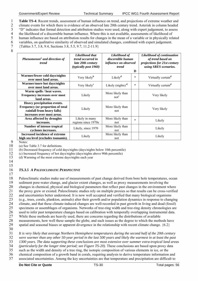
Government/Expert Review Technical Summary IPCC WG1 Fourth Assessment Report
1 2 3 4 5 6 7 8
Table TS-4. Recent trends, assessment of human influence on trend, and projections of extreme weather and climate events for which there is evidence of an observed late 20th century trend. Asterisk in column headed “D” indicates that formal detection and attribution studies were used, along with expert judgement, to assess the likelihood of a discernible human influence. Where this is not available, assessments of likelihood of human influence are based on attribution results for changes in the mean of a variable or in physically related variables, on qualitative similarity of observed and simulated changes, combined with expert judgement. {Tables 3.7, 3.8, 9.4, Sections 3.8, 5.5, 9.7, 11.2-11.9}
Phenomenona and direction of trend
Likelihood that trend occurred in late 20th century
(typically post 1960)
Likelihood of discernible human
influence on observed trend
Likelihood of continuation of trend based on
projections for 21st century using SRES scenarios.
D Warmer/fewer cold days/nights
over most land areas. Very likelyb Likelyd * Virtually certaind
Warmer/more hot days/nights over most land areas. Very likelyc Likely (nights) d * Virtually certaind
Warm spells / heat waves. Frequency increases over most
land areas. Likely More likely than
notc Very likely
Heavy precipitation events. Frequency (or proportion of total
rainfall from heavy falls) increases over most areas.
Likely More likely than not Very likely
Area affected by droughts increases.
Likely in many regions since 1970s
More likely than not * Likely
Number of intense tropical cyclones increases. Likely, since 1970 More likely than
not Likely
Increased incidence of extreme high sea level (excludes tsunamis). Likely More likely than
not Likely
9 10 11 12 13 14 15 16 17 18 19 20 21 22 23 24 25 26 27 28 29 30 31 32 33 34 35 36 37
Notes: (a) See Table 3.7 for definitions. (b) Decreased frequency of cold days/nights (days/nights below 10th percentile) (c) Increased frequency of hot days/nights (days/nights above 90th percentile) (d) Warming of the most extreme days/nights each year TS.3.5 A PALEOCLIMATIC PERSPECTIVE Paleoclimatic studies make use of measurements of past change derived from bore hole temperatures, ocean sediment pore-water change, and glacier extent changes, as well as proxy measurements involving the changes in chemical, physical and biological parameters that reflect past changes in the environment where the proxy grew or existed. Paleoclimatic studies rely on multiple proxies so that results can be cross-verified and uncertainties better understood. It is now well accepted and verified that many biological organisms (e.g., trees, corals, plankton, animals) alter their growth and/or population dynamics in response to changing climate, and that these climate-induced changes are well-recorded in past growth in living and dead (fossil) specimens or assemblages of organisms. Networks of tree-ring width and tree-ring density chronologies are used to infer past temperature changes based on calibration with temporally overlapping instrumental data. While these methods are heavily used, there are concerns regarding the distributions of available measurements, how well these sample the globe, and such issues as the degree to which the methods have spatial and seasonal biases or apparent divergence in the relationship with recent climate change. {6.2} It is very likely that average Northern Hemisphere temperatures during the second half of the 20th century were warmer than any other 50-year period in the last 500 years and likely the warmest in at least the past 1300 years. The data supporting these conclusions are most extensive over summer extra-tropical land areas (particularly for the longer time period; see Figure TS-20). These conclusions are based upon proxy data such as the width and density of a tree ring, the isotopic composition of various elements in ice, or the chemical composition of a growth band in corals, requiring analysis to derive temperature information and associated uncertainties. Among the key uncertainties are that temperature and precipitation are difficult to
Do Not Cite or Quote TS-30 Total pages: 56
Government/Expert Review Technical Summary IPCC WG1 Fourth Assessment Report
1 2 3 4 5 6 7 8 9
10 11 12 13 14 15 16 17 18 19 20 21 22 23 24 25 26 27 28 29 30 31 32 33 34 35 36 37 38 39 40 41 42 43 44 45 46 47 48 49 50 51 52 53 54 55 56 57
separate in some cases, or are representative of particular seasons rather than full years. There are now improved and expanded data since the TAR, including e.g., measurements at a larger number of sites, improved analysis of borehole temperature data, as well as more extensive analyses of glaciers, corals, and sediments. However, paleoclimatic data are more limited than the instrumental record since 1850 in both space and time, so that statistical methods are employed to construct global averages, and these are subject to uncertainties as well. Current data are too limited to allow a similar evaluation to be made for the Southern Hemisphere temperatures prior to the period of instrumental data. {6.6, 6.7} [INSERT FIGURE TS-20 HERE] Some post-TAR studies indicate greater multi-centennial Northern Hemisphere variability than was shown in the TAR, due to the particular proxies used, and the specific statistical methods of processing and/or scaling them to represent past temperatures. The additional variability implies cooler conditions, predominantly during the 12th to 14th, the 17th, and the 19th centuries; these are likely linked to natural forcings due to volcanic eruptions and/or solar activity. For example, reconstructions suggest decreased solar activity and increased volcanic activity in the 17th century as compared to current conditions. One reconstruction suggests slightly warmer conditions in the 11th century than those indicated in the TAR, but within the uncertainties quoted in the TAR. {6.6} The ice core CO2 record over the past millennium provides an additional constraint on natural climate variability. The amplitudes of the preindustrial, decadal-scale Northern Hemisphere temperature changes from the proxy-based reconstructions (<1°C) are broadly consistent with the ice core CO2 record and understanding of the strength of the carbon cycle-climate feedback. Atmospheric CO2 and temperature in Antarctica co-varied over the past 650,000 years. Available data suggest that CO2 acts as an amplifying feedback. {6.4, 6.6} Changes in glaciers are evident in Holocene data, but these changes were caused by different processes than the late 20th century retreat. Glaciers of several mountain regions in the Northern Hemisphere retreated in response to orbitally forced regional warmth between 11000 and 5000 years ago, and were smaller than at the end of the 20th century (or even absent) at times prior to 5000 years ago. The current near-global retreat of mountain glaciers cannot be due to the same causes, because decreased summer insolation during the past few thousand years in the Northern Hemisphere should be favourable to the growth of glaciers. {6.5} Paleoclimate data provide evidence for changes in many regional climates. The strength and frequency of ENSO events have varied in past climates. There is evidence that the strength of the Asian monsoon, and hence precipitation amount, can change abruptly. The paleoclimate records of northern and eastern Africa and of North America indicate that droughts lasting decades to centuries are a recurrent feature of climate in these regions, so that recent droughts in North America and Northern Africa are not unprecedented. Individual decadal-resolution paleoclimatic data support the existence of regional quasi-periodic climate variability, but it is unlikely that these regional signals were coherent at the global scale. {6.5, 6.6} Strong evidence from ocean sediment data and from modelling links abrupt climate changes during the last glacial period and glacial-interglacial transition to changes in the Atlantic Ocean circulation. Current understanding suggests that the ocean circulation can become unstable and change rapidly when critical thresholds are crossed. These events have affected temperature by up to 16oC in Greenland and have influenced tropical rainfall patterns. They were probably associated with a redistribution of heat between the northern and southern hemisphere rather than with large changes in global mean temperature. Such events have not been observed during the past 8000 years. {6.4} Confidence in the understanding of past climate change and changes in orbital forcing is strengthened by the improved ability of current models to simulate past climate conditions. The Last Glacial Maximum (LGM; the last 'ice age' about 21,000 years ago) and the mid-Holocene (6000 years ago) were different from the current climate not because of random variability, but because of altered seasonal and global forcing linked to known differences in the Earth's orbit (see Box TS.3.5). Biogeochemical and biogeophysical feedbacks amplified the response to orbital forcings. Comparisons between simulated and reconstructed conditions in the LGM demonstrate that models capture the broad features of inferred changes in the temperature and precipitation patterns. For the mid-Holocene, coupled climate models are able to simulate
Do Not Cite or Quote TS-31 Total pages: 56
Government/Expert Review Technical Summary IPCC WG1 Fourth Assessment Report
1 2 3 4
mid-latitude warming and enhanced monsoons, with little change in global mean temperature (<0.4°C), consistent with our understanding of orbital forcing. {6.2, 6.4, 6.5, 9.3}
5 BOX TS.3.5: ORBITAL FORCING 6
It is well known from astronomical calculations that periodic changes in characteristics of the Earth’s orbit 7 around the Sun control the seasonal and latitudinal distribution of incoming solar radiation at the top of the 8 atmosphere (hereafter called “insolation”). Past and future changes in insolation can be calculated over 9 several millions of years with a high degree of confidence {6.4}. 10
11 12 [INSERT BOX TS.3.5, FIGURE 1 HERE] 13
Precession refers to changes in the time of the year when the Earth is closest to the sun, with quasi-14 periodicities of about 19 and 23 kyr. As a result, changes in the position and duration of the seasons on the 15 orbit strongly modulate the latitudinal and seasonal distribution of insolation. Seasonal changes of insolation 16 are much larger than annual mean changes and can reach 60 W m–2 (Box TS.3.5, Figure 1). 17
18 The obliquity (tilt) of the Earth axis varies between about 22 and 24.5° with two neighbouring quasi-19 periodicities around 41 kyr. Changes in obliquity modulate seasonal contrasts as well as annual mean 20 insolation changes with opposite effects in low versus high latitudes (and therefore no effect on global 21 average of insolation) {6.4}. 22
23 The eccentricity of the Earth’s orbit around the Sun has longer quasi-periodicities at 400 kyr and around 100 24 kyr. Changes in eccentricity alone have limited impacts on insolation due to the resulting very small changes 25 in Sun-Earth distance. However, changes in eccentricity interact with seasonal effects induced by obliquity 26 and precession of the equinoxes. During periods of low eccentricity, such as ~400 kyr ago and during the 27 next 100 kyr, seasonal insolation changes induced by precession are less strong than during periods of larger 28 eccentricity (Box TS.3.5, Figure 1). {6.4} 29
30 The Milankovitch, or “orbital” theory of the ice ages is now well developed. Ice ages are generally triggered 31 by minima in high northern hemisphere summer insolation, enabling winter snowfall to persist through the 32 year and therefore accumulate to build northern hemisphere glacial ice sheets. Similarly, times with 33 especially intense high northern hemisphere summer insolation, determined by orbital changes, are thought 34 to trigger rapid deglaciations, associated climate change and sea level rise. These orbital forcings determine 35 the pacing of climatic changes, while the large responses appear to be determined by strong feedback 36 processes that amplify the orbital forcing. Over multi-millennial time scales, orbital forcing also exerts a 37 major influence on key climate systems such as the Earth’s major monsoons, global ocean circulation, as 38 well as the greenhouse gas content of the atmosphere. {6.4} 39
40 Available evidence indicates that the current warming will not be mitigated by a natural cooling trend 41 towards glacial conditions. Understanding of the Earth’s response to orbital forcing indicates that the earth 42 would not naturally enter another ice age for at least 30,000 years. {6.4, FAQ 6.1} 43
44 45 46 47 48 49 50 51 52 53 54
Global average sea level was likely between 4 and 6 m higher during the last interglacial period, about 125,000 years ago, than during the 20th Century (Figure TS-21), mainly due to the retreat of polar ice. Ice core data suggest that the Greenland Summit region was ice-covered in this period, but reductions in the ice sheet extent are indicated in parts of southern Greenland. Ice core data also indicate that average polar temperatures at that time were 3–5°C warmer than the 20th Century, because of differences in the Earth’s orbit. The Greenland ice-sheet and other Arctic ice fields likely contributed no more than 4 m of the observed sea level rise, implying that there may also have been a contribution from Antarctica. {6.4} [INSERT FIGURE TS-21 HERE]
Do Not Cite or Quote TS-32 Total pages: 56
Government/Expert Review Technical Summary IPCC WG1 Fourth Assessment Report
TS.4 UNDERSTANDING AND ATTRIBUTING CLIMATE CHANGE 1 2 3 4 5 6 7 8 9
10 11 12 13 14 15 16 17 18 19 20 21 22 23 24 25 26 27 28 29 30 31 32 33 34 35 36 37 38 39 40 41 42 43 44 45 46 47 48 49 50 51 52 53 54 55 56
Climate change is said to be detected when there is only a small likelihood that observed changes might have occurred solely due to natural variability. Attribution evaluates whether observed changes are consistent with quantitative responses to different forcings obtained in well-tested models, and are not consistent with alternative physically plausible explanations. The first IPCC Assessment Report (FAR; IPCC, 1990) contained little observational evidence of a detectable anthropogenic influence on climate. Six years later the IPCC Second Assessment Report (SAR; IPCC, 1996) concluded that the balance of evidence suggested a discernible human influence on the climate of the 20th century. The TAR concluded that “most of the observed warming over the last 50 years is likely to have been due to the increase in greenhouse gas concentrations”. Confidence in the assessment of the human contributions to recent climate change has increased considerably since the TAR, in part because of stronger signals obtained in longer records, as well as an expanded and improved range of observations to more fully address attribution of warming jointly with other changes in the climate system. Some apparent inconsistencies in the observational record (for example, that for the vertical profile of temperature changes) have been largely resolved. There have been improvements in the simulation of many aspects of present mean climate and its variability on seasonal to interdecadal timescales, although uncertainties remain (see Box TS.4.1). Models now employ more detailed representations of processes related to aerosol and other forcings. Simulations of 20th century climate change have used many more models and much more complete anthropogenic and natural forcings than were available in the TAR. Available multi-model ensembles increase confidence in attribution results by providing an improved representation of model uncertainty. An anthropogenic signal has now more clearly emerged in formal attribution studies of aspects of the climate system beyond global-scale atmospheric temperature, including changes in global ocean heat content, as well as continental scale temperature trends, temperature extremes, circulation and Arctic sea ice extent. {9.1} TS.4.1 ADVANCES IN ATTRIBUTION OF CHANGES IN GLOBAL SCALE TEMPERATURE IN THE
INSTRUMENTAL PERIOD: ATMOSPHERE, OCEAN AND ICE Anthropogenic warming of the climate system is widespread and can be detected in temperature observations taken at the surface, in the free atmosphere and in the oceans. {3.2, 3.4, 9.4} Evidence of the effect of external influences, both anthropogenic and natural, on the climate system has continued to accumulate since the TAR. Model and data improvements, ensemble simulations, and improved representations of aerosol and greenhouse gas forcing along with other influences lead to greater confidence that most current models reproduce large scale forced variability of the atmosphere on decadal and inter-decadal time scales quite well. These advances confirm that past climate variations on large spatial scales have been strongly influenced by external forcings. However, uncertainties still exist in the magnitude and temporal evolution of estimated contributions from individual forcings other than well-mixed greenhouse gases, due for example to uncertainties in model responses to forcing. Some potentially important forcings such as black carbon aerosols have not yet been considered in most formal detection and attribution studies. Uncertainties remain in estimates of natural internal climate variability. For example, there are discrepancies between estimates of ocean heat content variability from models and observations, although poor sampling of parts of the world ocean may explain this discrepancy. Also, internal variability is difficult to estimate from available observational records since these are influenced by external forcing, and because records are not long enough in the case of instrumental data, or precise enough in the case of proxy reconstructions, to provide complete descriptions of variability on decadal and longer time scales. (See Figure TS-22). {8.2, 8.3, 8.4, 8.6, 9.2, 9.3, 9.4, Box TS.4.1} [INSERT FIGURE TS-22 HERE] It is extremely unlikely (<5%) that the global pattern of warming observed during the past half century can be explained without external forcing. These changes took place over a time period when non-anthropogenic forcing factors (i.e., the sum of solar and volcanic forcing) would be likely to have produced cooling, not warming (See Figure TS-23). Attribution studies show that it is very likely that these natural forcing factors alone cannot account for the observed warming (See Figure TS-23). There is also increased confidence that natural internal variability cannot account for the observed changes, due in part to improved studies
Do Not Cite or Quote TS-33 Total pages: 56

Government/Expert Review Technical Summary IPCC WG1 Fourth Assessment Report
1 2 3 4 5 6 7 8 9
10 11 12 13 14 15 16 17 18 19 20 21 22 23 24
demonstrating that the warming occurred in both oceans and atmosphere, together with observed ice mass losses. {2.9, 3.2, 5.2, 9.4, 9.5, 9.7} [INSERT FIGURE TS-23 HERE] It is very likely that anthropogenic greenhouse gas increases caused most of the observed increase in globally averaged temperatures since the mid 20th century. Without the cooling effect of atmospheric aerosols, it is likely that greenhouse gases alone would have caused more global mean temperature rise than that observed during the last 50 years. A key factor in identifying the aerosol fingerprint, and therefore the amount of cooling counteracting greenhouse warming, is the temperature change through time (see Figure TS-23), as well as the hemispheric warming contrast. The conclusion that greenhouse gas forcing has been dominant takes into account observational and forcing uncertainties, and is robust to the use of different climate models, different methods for estimating the responses to external forcing, and different analysis techniques. It also allows for possible amplification of the response to solar forcing. {2.9, 6.6, 9.1, 9.2, 9.4} Widespread warming has been detected in ocean temperatures. Formal attribution studies now suggest that it is likely that anthropogenic forcing has contributed to the observed warming of the upper several hundred meters of the global ocean during the latter half of the 20th century. {5.2, 9.5} Anthropogenic forcing has likely contributed to recent decreases in Arctic sea ice extent. Changes in Arctic sea ice are expected given the observed enhanced Arctic warming. Attribution studies and improvements in the modelled representation of sea ice and in ocean heat transport strengthen the confidence in this conclusion. {3.3, 4.4, 8.2, 8.3, 9.5}
25 BOX TS.4.1: EVALUATION OF ATMOSPHERE-OCEAN GENERAL CIRCULATION MODELS 26
Atmosphere-ocean general circulation models (AOGCMs) are the primary tool used for understanding and 27 attribution of past climate variations, and for future projections. Since there are no historical perturbations to 28 radiative forcing that are fully analogous to the human-induced perturbations expected over the 21st Century, 29 confidence in the models must be built from a number of indirect methods, described below. In each of these 30 areas there have been substantial advances since the TAR, increasing overall confidence in models. {8.1} 31
32 Enhanced scrutiny and analysis of model behaviour has been facilitated by internationally coordinated 33 efforts to collect and disseminate output from model experiments performed under common conditions. This 34 has encouraged a more comprehensive and open evaluation of models, encompassing a diversity of 35 perspectives. {8.1} 36
37 Projections for different scales and periods using global climate models. Climate models project the climate 38 for several decades or longer into the future. Since the details of individual weather systems are not being 39 tracked and forecast, the initial atmospheric conditions are much less important than for weather forecast 40 models. For climate projections the forcings are of much greater importance. These forcings include the 41 amount of solar energy reaching the earth, the amount of particulate matter from volcanic eruptions in the 42 atmosphere, and the concentrations of anthropogenic gases and particles in the atmosphere. As the area of 43 interest moves from global to regional to local, or the timescale of interest shortens, the amplitude of 44 variability linked to weather increases relative to the signal of long term climate change. This makes 45 detection of the climate change signal more difficult at smaller scales. Conditions in the oceans are important 46 as well, especially for inter-annual and decadal time scales. {FAQ 1.2, 9.4, 11.1} 47
48 Model Formulation. The formulation of AOGCMs has developed through improved spatial resolution, and 49 improvements to numerical schemes and parameterisations (e.g., sea ice, atmospheric boundary layer, ocean 50 mixing). More processes have been included in many models, including a number of key processes 51 important for forcing (e.g., aerosols are now modelled interactively in many models). Most models now 52 maintain a stable climate without use of flux adjustments, although some long-term trends remain in 53 AOGCM control integrations, e.g., due to slow processes in the ocean. {8.2, 8.3} 54
55 Simulation of present climate. As a result of improvements in model formulation, there have been 56 improvements in the simulation of many aspects of present mean climate. Simulations of precipitation, sea 57
Do Not Cite or Quote TS-34 Total pages: 56
Government/Expert Review Technical Summary IPCC WG1 Fourth Assessment Report
level pressure and surface temperature have all improved overall, but deficiencies remain, notably in tropical 1 precipitation. While significant deficiencies remain in the simulation of cloud (and its feedbacks on climate 2 sensitivity), some models have demonstrated improvements in the simulation of certain cloud regimes 3 (notably marine stratocumulus). Simulation of extreme events (especially extreme temperature) has 4 improved, but models generally simulate too little precipitation in the most extreme events. Simulation of 5 extratropical cyclones has improved. Some models used for projections of tropical cyclone changes can 6 simulate successfully the observed frequency and distribution of tropical cyclones. Improved simulations 7 have been achieved in ocean water mass structure, MOC and ocean heat transport. However most models 8 show some biases in their simulation of the Southern Ocean, leading to some uncertainty in modelled ocean 9 heat uptake when climate changes. {8.3, 8.5, 8.6} 10
11 Simulation of modes of climate variability. Models simulate dominant modes of extratropical climate 12 variability which resemble the observed ones, NAM/SAM, PNA, PDO, but they still have problems in 13 representing aspects of them. Some models can now simulate important aspects of ENSO, while simulation 14 of the Madden-Julian Oscillation (MJO) remains generally unsatisfactory. {8.4} 15
16 Simulation of past climate variations. Advances have been made in the simulation of past climate variations. 17 Independently of any attribution of those changes, the ability of climate models to provide a physically self-18 consistent explanation of observed climate variations on various timescales builds confidence that the 19 models are capturing many key processes for the evolution of 21st Century climate. Recent advances include 20 success in modelling observed changes in a wider range of climate variables over the 20th Century (e.g., 21 continental-scale surface temperatures and extremes, sea ice extent, ocean heat content trends and land 22 precipitation). There has also been progress in the ability to model many of the general features of past, very 23 different climate states such as the Mid-Holocene and Last Glacial Maximum using identical or related 24 models to those used for studying current climate. Information on factors treated as boundary conditions in 25 paleoclimate calculations include the different states of ice sheets in those periods. The broad predictions of 26 earlier climate models, of increasing global temperatures in response to increasing greenhouse gases, have 27 been borne out by subsequent observations. This strengthens confidence in near-term climate projections and 28 understanding of related climate change commitments. {6.4, 6.5, 8.1, 9.3, 9.4, 9.5} 29
30 Weather and seasonal prediction using climate models. A few climate models have been tested for (and 31 shown) capability in initial value prediction, on timescales from weather forecasting (a few days) to seasonal 32 climate variations, when initialised with appropriate observations. While the predictive capability of models 33 in this mode of operation does not necessarily imply that they will show the correct response to changes in 34 climate forcing agents such as greenhouse gases, it does increase confidence that they are adequately 35 representing some key processes and teleconnections in the climate system {8.4} 36
37 Measures of model projection accuracy. The possibility of developing model capability measures 38 (‘metrics’), based on the above evaluation methods, that can be used to narrow uncertainty by providing 39 quantitative constraints on model climate projections, has been explored for the first time using model 40 ensembles. While these methods show promise, a proven set of measures has yet to be established. {8.1, 9.6, 41 10.5} 42
43 44 45 46 47 48 49 50 51 52 53 54 55 56 57
It is very likely that the response to anthropogenic forcing contributed to sea level rise during the latter half of the 20th century, but decadal variability in sea level rise remains poorly understood. Modelled estimates of the contribution to sea level rise from thermal expansion are in good agreement with estimates based on observations during 1961–2003, although the budget for sea level rise over that interval is not closed. The observed increase in the rate of loss of mass from glaciers and ice caps is proportional to the global average temperature rise expected from physical considerations (see Table TS-3). The greater rate of sea level rise in 1993–2003 than in 1961–2003 may be linked to increasing anthropogenic forcing, which has likely contributed to the observed warming of the upper ocean and widespread glacier retreat. On the other hand, the tide-gauge record of global mean sea level suggests that similarly large rates may have occurred in previous 10-year periods since 1950, implying that natural internal variability could also be a factor in the high rates for 1993–2003 period. Observed decadal variability in the tide-gauge record is larger than can be explained by variability in observationally based estimates of thermal expansion and land ice changes. Further, the observed decadal variability in thermal expansion is larger than simulated by models during the 20th century. Thus, the physical causes of the variability seen in the tide-gauge record are uncertain. These
Do Not Cite or Quote TS-35 Total pages: 56
Government/Expert Review Technical Summary IPCC WG1 Fourth Assessment Report
1 2 3 4 5 6 7 8 9
10 11 12 13 14 15 16 17 18 19 20 21 22 23 24 25 26 27 28 29 30 31 32 33 34 35 36 37 38 39 40 41 42 43 44 45 46 47 48 49 50 51 52 53 54 55 56 57
unresolved issues relating to sea level change and its decadal variability during 1961–2003 make it unclear how much of the higher rate of sea level rise in 1993–2003 is due to natural internal variability and how much to anthropogenic climate change. {5.5, 9.5} TS.4.2 ATTRIBUTION OF SPATIAL AND TEMPORAL CHANGES IN TEMPERATURE The observed pattern of tropospheric warming and stratospheric cooling can be largely attributed to the influence of anthropogenic forcing, particularly that due to greenhouse gas increases and stratospheric ozone depletion. New analyses since the TAR show that this pattern corresponds to an increase in the height of the tropopause that is likely due largely to greenhouse gas and stratospheric ozone changes. Significant uncertainty remains in the estimation of tropospheric temperature trends, particularly from the radiosonde record. {3.2, 3.4, 9.4} It is likely that there has been a substantial anthropogenic contribution to surface temperature increases averaged over every continent except Antarctica since the middle of the 20th century. Antarctica has insufficient observational coverage to make an assessment. Anthropogenic warming has also been identified in some sub-continental land areas. The ability of coupled climate models to simulate the temperature evolution on each of six continents provides stronger evidence of human influence on the global climate than was available in the TAR. No coupled global climate model that has used natural forcing only has reproduced the observed global mean warming trend, or the continental mean warming trends in individual continents (except Antarctica) over the second half of the 20th century. {9.4} Difficulties remain in attributing temperature changes on smaller than continental scales and over timescales of less than 50 years. Attribution results at these scales have, with limited exceptions, not been established. Averaging over smaller regions reduces the natural variability less than does averaging over large regions, making it more difficult to distinguish between changes expected from external forcing and variability. Also, temperature changes associated with some modes of variability are poorly simulated by models in some regions and seasons. Furthermore, the small-scale details of external forcing and the response simulated by models are less credible than large-scale features. {8.3, 9.4} Surface temperature extremes have likely been affected by anthropogenic forcing. Many indicators of extremes, including the annual numbers and most extreme values of warm and cold days and nights, as well as numbers of frost days, show changes that are consistent with warming. Anthropogenic influence has been detected in some of these indices, and there is evidence that anthropogenic forcing may have substantially increased the risk of extremely warm summer conditions regionally, such as the 2003 European heat wave. {9.4} TS.4.3 ATTRIBUTION OF CHANGES IN CIRCULATION, PRECIPITATION AND OTHER CLIMATE VARIABLES Trends in the Northern and Southern Annular Modes over recent decades, which correspond to sea level pressure reductions over the poles and related changes in atmospheric circulation, are likely related in part to human activity. (See Figure TS-24.) Models reproduce the sign of the Northern Annular Mode trend, but the simulated response is smaller than observed. Models including both greenhouse gas and stratospheric ozone changes simulate a realistic trend in the Southern Annular Mode, leading to a detectable human influence on global sea level pressure that is also consistent with the observed cooling trend in surface climate over parts of Antarctica. These changes in hemispheric circulation and their attribution to human activity imply that anthropogenic effects have likely contributed to changes in mid- and high-latitude patterns of circulation and temperature, as well as changes in winds and storm tracks. However, quantitative effects are uncertain because simulated responses to 20th century forcing change for the Northern Hemisphere agree only qualitatively and not quantitatively with observations of these variables. {3.6, 9.5, 10.3} [INSERT FIGURE TS-24 HERE] There is some evidence of the impact of external influences on the hydrological cycle. The observed large-scale pattern of changes in land precipitation over the 20th century are qualitatively consistent with simulations, suggestive of a human influence. An observed global trend towards increases in drought in the second half of the 20th century has been reproduced with a model by taking anthropogenic and natural forcing into account. A number of studies have now demonstrated that changes in land use, due for example
Do Not Cite or Quote TS-36 Total pages: 56
Government/Expert Review Technical Summary IPCC WG1 Fourth Assessment Report
to overgrazing and conversion of woodland to agriculture, are unlikely to have been the primary cause of Sahelian and Australian droughts. Comparisons between observations and models suggest that changes in monsoons, storm intensities, and Sahelian rainfall are related at least in part to changes in observed sea surface temperatures. Changes in global SSTs are expected to be affected by anthropogenic forcing, but an association of regional SST changes with forcing has not been established. Changes in rainfall depend not just upon SSTs but also upon changes in the spatial and temporal SST patterns and regional changes in atmospheric circulation, making attribution to human influences difficult. {3.3, 9.5, 10.3, 11.2}
1 2 3 4 5 6 7 8 9
10 11 12 13 14 15 16 17 18 19 20 21 22 23 24 25 26 27 28 29 30 31 32 33 34 35 36 37 38 39 40 41 42 43 44 45 46 47 48 49 50 51 52 53 54 55
TS.4.4 PALEOCLIMATE STUDIES OF ATTRIBUTION It is very likely that climate changes of at least the seven centuries prior to 1950 were not due to unforced variability alone. Detection and attribution studies indicate that a substantial fraction of pre-industrial Northern Hemisphere interdecadal temperature variability contained in reconstructions for those centuries is very likely attributable to natural external forcing. Such forcing includes: episodic cooling due to known volcanic eruptions, a number of which were larger than those of the 20th century (based on evidence such as ice cores); and long-term variations in solar irradiance, such as reduced radiation during the Maunder Minimum. Further, it is likely that anthropogenic forcing contributed to the early 20th century warming evident in these records. Uncertainties are unlikely to lead to a spurious agreement between temperature reconstructions and forcing reconstructions as they are derived from independent proxies. Insufficient data are available to make a similar Southern Hemisphere evaluation. {6.6, 9.3} TS.4.5 CLIMATE RESPONSE TO RADIATIVE FORCING Specification of a likely range and a most likely value for equilibrium climate sensitivity7 in this report represents significant progress in quantifying the climate system response to radiative forcing since the TAR and an advance on challenges to understanding that have persisted for over 30 years. The likely range for equilibrium climate sensitivity, the equilibrium global average warming expected if CO2 concentrations were to be sustained at double their pre-industrial values (about 550 ppmv), was estimated in the TAR to likely be between 1.5 to 4.5°C and in previous assessments it was not possible to provide a best estimate and to estimate the probability that climate sensitivity might fall outside the quoted range. Several approaches are used in this assessment to constrain climate sensitivity including the use of AOGCMs, examination of the transient evolution of temperature (surface, upper air, , and ocean) over the last 150 years and the rapid response of the global climate system to changes in the forcing caused by volcanic eruptions (See Figure TS-25). These are complemented by estimates based upon paleoclimate studies such as reconstructions of the Northern Hemisphere temperature record of the past millennium and the Last Glacial Maximum. Large ensembles of climate model simulations have shown that the ability of models to simulate present climate has value in constraining climate sensitivity. {8.1, 8.6, 9.6, Box 10.2} [INSERT FIGURE TS-25 HERE] Analysis of models together with constraints from observations suggest that the equilibrium climate sensitivity is likely to be in the range 2–4.5°C, with a best estimate value of about 3°C. It is very unlikely to be less than 1.5°C. Values substantially higher than 4.5°C cannot be excluded, but agreement with observations is not as good for those values. Probability density functions (PDFs) derived on the basis of different information and approaches generally tend to have a long tail toward high values exceeding 4.5°C. Analysis of climate and forcing evolution over previous centuries and model ensemble studies do not rule out climate sensitivity being as high as 6°C or more. One factor in this is the possibility of small net radiative forcing over the 20th century if aerosol indirect cooling effects were at the upper end of their uncertainty range, thus cancelling most of the positive forcing due to greenhouse gases. However, there is no well established way of estimating a single PDF from individual results taking account of the different assumptions in each study. The lack of strong constraints limiting high climate sensitivities prevents the specification of a 95%-ile bound or a very likely range for climate sensitivity. {Box 10.2} There is now increased confidence in the understanding of key climate processes that are important to climate sensitivity due to improved analyses and comparisons of models to one another and to observations.
7 See the Glossary for a detailed definition of climate sensitivity. Do Not Cite or Quote TS-37 Total pages: 56

Government/Expert Review Technical Summary IPCC WG1 Fourth Assessment Report
Water vapour changes dominate the feedbacks affecting climate sensitivity and are now better understood. New observational and modelling evidence strongly favours a combined water vapour – lapse rate
1 2 3 4 5 6 7 8 9
10 11 12 13 14 15 16 17 18 19 20 21 22 23 24 25 26 27
8 feedback of around the strength found in General Circulation Models (GCMs) i.e. approximately 1 W m–2 per degree global temperature increase, corresponding to about a 50% amplification of global mean warming. Such GCMs have demonstrated an ability to simulate seasonal to inter-decadal humidity variations in the upper troposphere over land and ocean, and have successfully simulated the observed surface temperature and humidity changes associated with volcanic eruptions. Cloud feedbacks (particularly from low clouds) remain the largest source of uncertainty. Cryospheric feedbacks such as changes in snow cover have been shown to contribute less to the spread in model estimates of climate sensitivity than cloud or water vapour feedbacks, but they can be important for regional climate responses at mid- and high-latitudes. A new model intercomparison suggests that differences in radiative-transfer formulations also contribute to the range. {3.4, 8.6, 9.3, 9.4, 9.6, 10.2, Box 10.2} Improved quantification of climate sensitivity allows estimation of best estimate equilibrium temperatures and ranges that could be expected if concentrations of carbon dioxide were to be stabilized at various levels based on global energy balance considerations (see Table TS-5). As in the estimate of climate sensitivity, a very likely upper bound cannot be established. Limitations to the concept of radiative forcing and climate sensitivity should be noted. Only a few AOGCMs have been run to equilibrium under elevated CO2 concentrations, and some results show that climate feedbacks may change over long time scales, resulting in substantial deviations from estimates of warming based on equilibrium climate sensitivity inferred from mixed-layer ocean models and past climate change. {10.7} Table TS-5. Best estimate, likely and very likely bounds/ranges of global mean equilibrium surface temperature increase ΔT (°C) over pre-industrial temperatures for different levels of CO2 equivalent radiative forcing, as derived from the climate sensitivity.
Eq CO2 best estimate very likely above likely in the range
350 1.0 0.5 0.6–1.4 450 2.1 1.0 1.4–3.1 550 2.9 1.5 1.9–4.4 650 3.6 1.8 2.4–5.5 750 4.3 2.1 2.8–6.4
1000 5.5 2.8 3.7–8.3 1200 6.3 3.1 4.2–9.4
28 29 30 31 32 33 34 35 36 37 38 39 40 41 42 43 44 45
Agreement among models for projected transient climate change has also improved since the TAR. The range of transient climate responses (defined as the globally averaged surface air temperature averaged over a 20 year period centered at the time of CO2 doubling in a 1%/year increase experiment) among models is smaller than the range in the equilibrium climate sensitivity. This parameter is now better constrained by multi-model ensembles and comparisons with observations; it is very likely to be greater than 1°C and very unlikely to be greater than 3°C. The transient climate response is related to sensitivity in a non-linear way such that high sensitivities are not immediately manifested in the short-term response. Transient climate response is strongly affected by the rate of ocean heat uptake. Although the ocean models have improved, systematic model biases and limited ocean temperature data to evaluate transient ocean heat uptake affect the accuracy of current estimates. {8.3, 8.6, 9.4, 9.6, 10.5} TS.5 PROJECTIONS OF FUTURE CHANGES IN CLIMATE Since the TAR, there have been many important advances in the science of climate change projections. An unprecedented effort has been initiated to make new model results available for prompt scrutiny by researchers outside the modelling centers. A set of coordinated, standard experiments was performed by
8 The rate at which air temperature decreases with altitude. Do Not Cite or Quote TS-38 Total pages: 56

Government/Expert Review Technical Summary IPCC WG1 Fourth Assessment Report
fourteen Atmosphere-Ocean General Circulation Model (AOGCM) modelling groups from ten countries using 23 models. The resulting multi-model database of outputs, analyzed by hundreds of researchers worldwide, form the basis for much of this assessment of model results.
1 2 3 4 5 6 7 8 9
10 11 12 13 14 15 16 17 18 19 20 21 22 23 24 25 26 27 28 29 30 31 32 33 34 35 36 37 38 39 40 41 42 43 44
Many advances have come from the use of multi-member ensembles from single models, e.g. to test the sensitivity of response to initial conditions, and from multi-model ensembles. These two different types of ensembles allow more robust studies of the range of model results and more quantitative model evaluation against observations, as well as new information on simulated statistical variability. {8.1, 8.3, 9.4, 9.5, 10.1} A number of methods for providing probabilistic climate change projections, both for global means and geographical depictions, have emerged since the TAR and are a focus of this report. These include methods based on results of AOGCM ensembles without formal application of observational constraints as well as methods based on detection algorithms and on large model ensembles that provide projections consistent with observations of climate change and their uncertainties. Some methods now explicitly account for key uncertainty sources such as climate feedbacks, ocean heat uptake, radiative forcing, and the carbon cycle. Short-term projections are similarly constrained by observations of recent trends. Some studies have probed additional probabilistic issues such as the likelihood of future changes in extremes such as heat waves that could occur due to human influences. Advances have also occurred since the TAR through new studies of how climate is likely to change through broader ranges of studies of committed climate change, and of carbon-climate feedbacks. {8.6, 9.6, 10.1, 10.3, 10.5} These advances in the science of climate change modelling provide a probabilistic basis for distinguishing projections of climate change for different SRES marker scenarios. This is in contrast to the TAR where ranges for different marker scenarios could not be given in probabilistic terms. As a result, this assessment identifies and quantifies the difference in character between uncertainties that arise in climate modelling and those that arise from a lack of prior knowledge of decisions that will affect greenhouse gas emissions. Loss of policy relevant information would result from combining probabilistic projections. For these reasons, projections for different emission scenarios will not be combined in this report. Model simulations used here consider the response of the physical climate system to a range of possible future conditions through use of idealised emissions or concentration assumptions. These include experiments with greenhouse gases and aerosols held constant at year 2000 levels, CO2 doubling and quadrupling experiments, SRES9 marker scenarios for the 2000–2100 period, and experiments with greenhouse gases and aerosols held constant after 2100, providing new information on the physical aspects of long term climate change and stabilization. The SRES scenarios did not include climate initiatives. This Working Group I assessment does not evaluate the plausibility or likelihood of any specific emission scenario. {10.1, 10.3} A new multi-model dataset using Earth system Models of Intermediate Complexity (EMICs) complements AOGCM experiments to extend the time horizon for several more centuries in the future. This provides a more comprehensive range of model responses in this assessment as well as new information on climate change over long time scales when greenhouse gas and aerosols concentrations are held constant. Some AOGCMs and EMICs contain prognostic carbon cycle components, which permit the estimation of the likely effects and associated uncertainties of carbon cycle feedbacks. {10.1}
45 BOX TS.5.1: HIERARCHY OF GLOBAL CLIMATE MODELS 46
Estimates of change in global mean temperature and sea level rise due to thermal expansion can be made 47 using simple climate models (SCMs) that represent the ocean-atmosphere system as a set of global or 48 hemispheric boxes, and predict global surface temperature using an energy balance equation, a prescribed 49 value of climate sensitivity and a basic representation of ocean heat uptake. Such models can also be coupled 50 to simplified models of biogeochemical cycles and allow rapid estimation of the climate response to a wide 51 range of emission scenarios. {8.8, 10.5} 52 53
9 SRES refers to the IPCC Special Report on Emission Scenarios. The SRES scenario families and illustrative cases are summarized in a box at the end of the Summary for Policymakers. Do Not Cite or Quote TS-39 Total pages: 56
Government/Expert Review Technical Summary IPCC WG1 Fourth Assessment Report
Earth System Models of Intermediate Complexity (EMICs) include some dynamics of the atmospheric and 1 oceanic circulations, or parameterisations thereof, and often include representations of biogeochemical 2 cycles, but they commonly have reduced spatial resolution. EMICs can be used to investigate continental 3 scale climate change and long term large scale effects of coupling between Earth system components using 4 large ensembles of model runs or runs over many centuries. For both SCMs and EMICs it is computationally 5 feasible to sample parameter spaces thoroughly taking account of parameter uncertainties derived from 6 tuning to more comprehensive climate models, matching observations, and use of expert judgment. Thus 7 both types of model are well suited to the generation of probabilistic projections for future climate and allow 8 a comparison of the ‘response uncertainty’ arising from uncertainty in climate model parameters with 9 ‘scenario range’ arising from the range of emission scenarios being considered. EMICs have been evaluated 10 in greater depth than previously and intercomparison exercises have demonstrated that they are useful for 11 studying questions involving long timescales or requiring large ensembles of simulations. {8.8, 10.5, 10.7} 12
13 The most comprehensive climate models are the AOGCMs. They include dynamical components describing 14 atmospheric, oceanic, and land suface processes, as well as sea ice, and other components. Much progress 15 has been made since the TAR (see Box TS.4.1) and there are over 20 models from different centers available 16 for climate simulations. Although the large scale dynamics of these models are comprehensive, 17 parameterisations are still used to represent unresolved physical processes such as, e.g., the formation of 18 clouds and precipitation, ocean mixing due to wave processes and the formation of water masses, etc. 19 Uncertainty in parameterisations is the primary reason why climate projections differ between different 20 AOGCMs. While resolution of AOGCMs is rapidly improving, it is often insufficient to capture fine-scale 21 structure of climatic variables in many regions. In such cases the output from AOGCMs can be used to drive 22 limited-area (or regional climate) models that combine comprehensiveness of process representations 23 comparable to AOGCMs with much higher spatial resolution. {8.2} 24
25 26 27 28 29 30 31 32 33 34 35 36 37 38 39 40 41 42 43 44 45 46 47 48 49 50 51 52 53 54 55
TS.5.1 UNDERSTANDING NEAR TERM CLIMATE CHANGE Our knowledge of the climate system together with model simulations confirms that past changes in greenhouse gas concentrations will lead to a committed warming (see Box TS.5.2 for a definition) and future climate change. New model results for experiments in which concentrations of all forcing agents were held constant provide better estimates of the committed changes in atmospheric variables that would follow because of the long response time of the climate system, particularly the oceans. {10.3, 10.7} Previous IPCC projections of future climate changes can now be compared to recent observations, increasing confidence in short term projections and the underlying physical understanding of committed climate change over a few decades. Projections for 1990-2005 carried out for the IPCC’s first and second assessment reports suggested global mean temperature increases of about 0.3°C and 0.15°C per decade, respectively10. The difference between the two was due primarily to the inclusion of aerosol cooling effects in the second assessment, whereas there was no quantitative basis for doing so in the first assessment; projections given in the TAR were similar to those of the SAR. These results are comparable to observed values of about 0.2°C per decade, as shown in Figure TS-26, providing broad confidence in such short-term projections. Some of this warming is the committed effect of changes in the concentrations of greenhouse gases prior to the times of those earlier assessments. {1.2, 3.2} [INSERT FIGURE TS-26 HERE] Committed climate change (see Box TS.5.2) due to atmospheric composition in the year 2000 corresponds to a warming trend of about 0.1°C per decade over the next two decades, in the absence of large changes in volcanic or solar forcing. About twice as much warming (0.2°C per decade) would be expected if emissions were to fall within the range of the SRES marker scenarios. This result is insensitive to the choice among the SRES marker scenarios, none of which considered climate initiatives. By 2050, the range of expected warming shows limited sensitivity to the choice among SRES scenarios (1.3°C to 1.7°C relative to 1980-1999) with about a quarter being due to the committed climate change if all radiative forcing agents were stabilized today. {10.3, 10.5, 10.7}
10 See IPCC First Assessment Report, Policymakers Summary, and Second Assessment Report, Technical Summary, Figure 18. Do Not Cite or Quote TS-40 Total pages: 56

Government/Expert Review Technical Summary IPCC WG1 Fourth Assessment Report
1 BOX TS.5.2: COMMITTED CLIMATE CHANGE 2
If the concentrations of greenhouse gases and aerosols were held fixed after a period of change, the climate 3 system would continue to respond due to the thermal inertia of the oceans and ice sheets and their long time 4 scales for adjustment. Committed warming is defined here as the further change in global mean temperature 5 after atmospheric composition, and hence radiative forcing, is held constant. Committed change also 6 involves other aspects of the climate system, in particular sea level. Note that holding concentrations of 7 radiatively active species constant would imply that ongoing emissions match natural removal rates, which 8 for most species would be equivalent to a large reduction in emissions and the corresponding model 9 experiments are not intended to be considered as emission scenarios. {FAQ 10.3} 10
11 The troposphere adjusts to changes in its boundary conditions on time scales shorter than a month or so. The 12 upper ocean responds with time scales of several years to decades, with the deep ocean and ice sheet 13 response time scales being from centuries to millennia. When the radiative forcing changes the atmosphere 14 tries to adjust quickly. However, because the atmosphere is strongly coupled to the oceanic mixed layer, 15 which in turn is coupled to the deeper oceanic layer, it takes a very long time for the atmospheric variables to 16 come to an equilibrium. During the long periods where the surface climate is changing very slowly, one can 17 consider that the atmosphere is in a quasi-equilibrium state, and most energy is being absorbed by the ocean, 18 so that ocean heat uptake is a key measure of climate change. {10.7} 19
20 21 22 23 24 25 26 27 28 29 30 31 32 33 34 35 36 37 38 39 40 41 42 43 44 45 46 47 48 49 50 51 52
Sea level is expected to continue to rise in the next several decades. During 2000–2020 under scenario SRES A1B in the ensemble of AOGCMs, the rate of thermal expansion is projected to be 1.3 ± 0.7 mm yr–1, and is not significantly different under A2 or B1. These projected rates are within the uncertainty of the observed contribution of thermal expansion for 1993–2003 of 1.6 ± 0.6 mm yr-1. Committed thermal expansion linked to atmospheric composition in the year 2000 represents a larger fraction of future thermal expansion driven sea level rise than for global average surface temperature. {10.6, 10.7} TS.5.2 LARGE SCALE PROJECTIONS FOR THE 21ST CENTURY This section covers advances in understanding global-scale climate projections and the processes that influence their large-scale patterns in the 21st century. More specific discussion of regional-scale changes follows in section 5.3. Projected globally-averaged surface warming for the end of the 21st century (2090–2099) is scenario-dependent and the actual warming will be significantly affected by the actual emissions that occur. Warmings compared to 1980–1999 for six SRES scenarios11, given as best estimates and corresponding likely ranges, are: B1: 1.7 (1.0–2.7)°C; A1T: 2.4 (1.4–3.8)°C; B2: 2.4 (1.4–3.8)°C; A1B: 2.7 (1.6–4.3)°C; A2: 3.2 (1.9–5.1)°C; A1FI: 4.0 (2.4–6.3)°C. These results are based on AOGCMs, observational constraints and other methods to quantify the range of model response (see Figure TS-27). The combination of multiple lines of evidence allows a likelihood to be assigned to the resulting ranges, representing an important advance since the TAR. {10.5} [INSERT FIGURE TS-27 HERE] Assessed uncertainty ranges are larger than those given in the TAR because they consider a more complete range of models and climate carbon-cycle feedbacks. Warming tends to reduce land and ocean uptake of atmospheric carbon dioxide, increasing the fraction of anthropogenic emissions that remains in the atmosphere. For the A2 scenario for example, the carbon dioxide feedback increases the corresponding global average warming at 2100 by more than 1°C. {7.3, 10.5} Projected globally-averaged sea level rise at the end of the 21st century (2090–2099), relative to 1980–1999 for the six SRES marker scenarios, given as best estimates and 5%–95% ranges based on the spread of
11 Approximate CO2 equivalent concentrations corresponding to the computed radiative forcing due to anthropogenic greenhouse gases and aerosols in 2100 (see p. 823 of the TAR) for the SRES B1, A1T, B2, A1B, A2 and A1FI illustrative marker scenarios are about 600, 700, 800, 850, 1250 and 1550 ppm respectively. Constant emission at year 2000 levels would lead to a concentration for CO2 alone of about 520 ppm by 2100. Do Not Cite or Quote TS-41 Total pages: 56
Government/Expert Review Technical Summary IPCC WG1 Fourth Assessment Report
AOGCM results, are: B1: 0.28 (0.19–0.37) m; A1T 0.33 (0.22–0.44) m; B2: 0.32 (0.21–0.42) m; A1B: 0.35 (0.23–0.47) m; A2: 0.37 (0.25–0.50) m; A1FI: 0.43 (0.28–0.58) m. Improved observations of recent mass loss from glaciers has narrowed the uncertainty relative to the TAR, contributing to a reduced upper bound. Thermal expansion contributes 60%–70% to the best estimate for each scenario. An additional improvement since the TAR is the use of AOGCMs to evaluate ocean heat uptake and thermal expansion. This has also reduced the upper bound as compared to the simple model used in the TAR. In all SRES scenarios, the average rate of sea level rise during the 21st century very likely exceeds the 1961–2003 average rate (1.8 ± 0.5 mm yr
1 2 3 4 5 6 7 8 9
10 11 12 13 14 15 16 17 18 19 20 21 22 23 24 25 26 27 28 29 30 31 32 33 34 35 36 37 38 39 40 41 42 43 44 45 46 47 48 49 50 51 52 53 54 55 56 57
–1). For an average model, the scenario spread in sea level rise is only 0.02 m by the middle of the century, but by the end of the century it is 0.15 m. These ranges do not include uncertainties in carbon-cycle feedbacks or ice flow processes because a basis in published literature is lacking. {10.6, 10.7} Changes in the cryosphere will continue to affect sea level rise during the 21st century. Glaciers, ice caps and the Greenland ice sheet are projected to lose mass in the 21st century because increased melting will exceed increased snowfall. Current models suggest that the Antarctic ice sheet will remain too cold for widespread melting and may gain mass in future through increased snowfall, acting to reduce sea level rise. However, changes in ice dynamics could increase the contributions of both Greenland and Antarctica to 21st century sea level rise. Recent observations of some Greenland outlet glaciers give strong evidence for enhanced flow when ice shelves are removed. The observation in west-central Greenland of seasonal variation in ice flow rate and of a correlation with summer temperature variation suggest that surface meltwater may join a subglacially routed drainage system lubricating the ice flow. By both these mechanisms, greater surface melting during the 21st century could cause acceleration of ice flow and discharge and increase the sea level contribution. In some parts of West Antarctica, large accelerations of ice flow have recently occurred, which may have been caused by thinning of ice shelves due to ocean warming. Although this has not been formally attributed to anthropogenic climate change due to greenhouse gases, it suggests that future warming could cause faster loss of mass and greater sea level rise. Quantitative projections of this effect cannot be made with confidence. If recently observed increases in ice discharge rates from the Greenland and Antarctic ice sheets were to increase linearly with global average temperature change that would add 10–25% to the central estimate of sea level rise for each scenario given above. Understanding of these effects is too limited to allow a best estimate to be made. {4.6, 10.6} Many of the global and regional patterns of temperature and precipitation seen in the TAR projections remain in the new generation of models and across ensemble results (see Figure TS-28). Confidence in the robustness of these patterns is increased by the fact that they have remained largely unchanged while overall model simulations have improved (Box TS.4.1). This adds to confidence that these patterns reflect basic physical constraints on the climate system as it warms {8.3, 8.4, 8.5, 10.3, 11.2-11.9} The projected 21st century temperature change is positive everywhere. It is maximum in high latitudes and over land in Northern hemisphere during winter and increases as one moves away from coasts and into the continental interiors. In otherwise geographically similar areas, warming is typically larger in arid than in moist regions. {10.3, 11.2-11.9} In contrast, warming is least over the southern oceans and the North Atlantic. Temperatures are projected to warm including over the North Atlantic and Europe despite a projected slowdown of the MOC in most models, due to the much larger influence of the increase of greenhouse gases. The projected pattern of zonal mean temperature change in the atmosphere displays a maximum warming in the upper tropical troposphere and cooling in the stratosphere. Further zonal mean warming in the ocean is expected to occur first near the surface and in the northern mid-latitudes, with the warming gradually reaching the ocean interior, most evident at high-latitudes where vertical mixing is greatest. The projected pattern of change is very similar among the late century cases irrespective of the scenario. Zonally averaged fields normalized by the mean warming are very similar for the scenarios examined (see Figure TS-28.) {10.3} [INSERT FIGURE TS-28 HERE] It is very likely that the Atlantic meridional overturning circulation (MOC) will slow down over the course of the 21st century, with an average model-estimated reduction by 2100 of 25% (range from zero to more than 50%). The projected reduction of the Atlantic MOC is due to the combined effects of an increase of high latitude temperatures and precipitation, which reduce the density of the surface waters in the North Atlantic.
Do Not Cite or Quote TS-42 Total pages: 56
Government/Expert Review Technical Summary IPCC WG1 Fourth Assessment Report
1 2 3 4 5 6 7 8 9
10 11 12 13 14 15 16 17 18 19 20 21 22 23 24 25 26 27 28 29 30 31 32 33 34 35 36 37 38 39 40 41 42 43 44 45 46 47 48 49 50 51 52 53 54 55 56 57
Very few AOGCM studies have included the impact of additional fresh water from melting of the Greenland Ice Sheet, but those that have do not suggest that this will lead to a complete MOC shutdown. Taken together, it is likely that the MOC will reduce, perhaps associated with a significant reduction in Labrador Sea Water formation, but very unlikely that the MOC will undergo a large abrupt transition during the course of the 21st century. {8.7, 10.3} Models indicate that sea level rise during the 21st century will not be geographically uniform. Under scenario A1B for 2070–2099, AOGCMs give a median spatial standard deviation of 0.08 m, which is about 25% of the central estimate of the global average sea level rise. The geographical patterns of future sea level change arise mainly from changes in the distribution of heat and salinity in the ocean and consequent changes in ocean circulation. Projected patterns display more similarity across models than those analysed in the TAR. Common features are a smaller than average sea level rise in the Southern Ocean, larger than average in the Arctic, and a narrow band of pronounced sea level rise stretching across the southern Atlantic and Indian Oceans. {10.6} Projections of changes in extremes such as the frequency of heat waves are better quantified than in the TAR, due to improved models and a better assessment of model spread based on multi-model ensembles. The TAR concluded there was a risk of increased temperature extremes, with more extreme heat episodes in a future climate. This result has been confirmed and expanded in more recent studies. Future increases in temperature extremes are projected to follow increases in mean temperature over most of the world except where surface properties (e.g. snow cover or soil moisture) change. A multi-model analysis, based on simulations of 14 models for 3 scenarios, investigated changes in extreme seasonal (DJF and JJA) temperatures where extreme is defined as lying above the 95%-ile of the simulated temperature distribution for the 20th century. By the end of the 21st century the projected probability of extreme warm seasons rises above 90% in many tropical areas, and reaches around 40% elsewhere. Several recent studies have addressed possible future changes in heat waves, and found that, in a future climate, heat waves are expected to be more intense, longer-lasting and more frequent. Based on an 8 member multi-model ensemble, heat waves are simulated to have been increasing for the latter part of the 20th century, and are projected to increase globally and over most regions. {8.5, 10.3} For a future warmer climate, models project a decline in frequency of cold air outbreaks relative to the present of 50 to 100% in Northern Hemisphere winter in most areas. Results from a 9 member multi-model ensemble show simulated decreases in frost days for the 20th century continuing into the 21st century globally and in most regions. A quantity related to frost days is growing season length and this has been projected to increase in future climate. {10.3, FAQ 10.1} Snow cover is projected to decrease. Widespread increases in thaw depth over most permafrost regions are projected to occur. {10.3} Under several different scenarios (SRES A1B, A2 and B1) large parts of the Arctic ocean are expected to no longer have year-round ice cover by the end of the 21st century. Arctic sea ice responds sensitively to warming. While projected changes in winter sea ice extent are moderate, late summer sea ice is projected to disappear almost completely towards the end of the 21st century under the A2 scenario in some models. The reduction is accelerated by a number of positive feedbacks in the climate system. The ice albedo feedback allows open water to receive more heat from the sun during summer, the insulating effect of sea ice is reduced, and the increase of ocean heat transport to the Arctic further reduces ice cover. Model simulations indicate that the late summer sea ice cover reduces substantially and generally evolves on the same time scale as global warming. Antarctic sea ice extent is also projected to decrease in the 21st century. {8.6, 10.3, Box 10.1} Sea level pressure is projected to increase over the subtropics and mid-latitudes, and decrease over high-latitudes associated with an expansion of the Hadley Circulation and annular mode changes (NAM/NAO, and SAM). There is a positive trend of the NAM/NAO as well as the SAM index projected by many models. The magnitude of the projected increase is generally greater for the SAM, and there is considerable spread among the models. As a result of these changes, storm tracks are projected to move poleward, with consequent changes in wind, precipitation, and temperature patterns outside the tropics, continuing the broad pattern of observed trends over the last half-century. Some studies suggest fewer storms in mid-latitude
Do Not Cite or Quote TS-43 Total pages: 56

Government/Expert Review Technical Summary IPCC WG1 Fourth Assessment Report
1 2 3 4 5 6 7 8 9
10 11 12 13 14 15 16 17 18 19 20 21 22 23 24 25 26 27 28 29 30 31 32 33 34 35 36 37 38 39 40 41 42 43 44 45 46 47 48 49 50 51 52 53 54 55 56 57
regions. There are also indications of changes in extreme wave height associated with changing storm tracks and circulation {3.6, 10.3} In most models the central and eastern equatorial Pacific sea surface temperatures warm more than the western equatorial Pacific, with a corresponding mean eastward shift of precipitation. ENSO interannual variability is projected to continue in all models, although changes differ from model to model. Large inter-model differences in projected changes of El Niño amplitude, and the inherent century-timescale variability of El Niño in the models, preclude a definitive projection of trends in ENSO variability. {10.3} Recent studies with improved global models, ranging in resolution from about 100 to 20 km suggest future changes in number and intensity of future tropical cyclones (typhoons and hurricanes). A synthesis of the model results to date indicates, for a warmer future climate, increased peak wind intensities and increased mean and peak precipitation intensities in future tropical cyclones, with the possibility of a decrease in the number of relatively weak hurricanes, and increased numbers of intense hurricanes. However, the total number of tropical cyclones globally is projected to decrease. The apparent observed 20th century increase in the proportion of very intense hurricanes is in the same direction but much larger than predicted by theoretical models. {10.3, 8.5, 3.8} Since the TAR there is an improving understanding of projected patterns of precipitation. Increases in the amount of precipitation are very likely in high-latitudes while decreases are likely in most subtropical land regions (by as much as about 20% in the A1B scenario in 2100). Poleward of 50 degrees, mean precipitation is projected to increase due to the increase in water vapour in the atmosphere and the resulting increase in vapour transport from lower latitudes. Moving equatorwards, there is a transition to mostly decreasing precipitation in the subtropics (20-40 degrees latitude). Due to increased water vapor transport out of the subtropics and a poleward expansion of the subtropical high pressure systems, the drying tendency is especially pronounced at the higher latitude margins of the subtropics. (See Figure TS-30). {8.3, 10.3, 11.2-11.9} Models suggest that changes in mean precipitation amount, even where robust, will rise above natural variability more slowly than the temperature signal. {10.3, 11.1} Available research indicates a tendency for an increase in heavy daily rainfall events in many regions, including some in which the mean rainfall is projected to decrease. In the latter, the rainfall decrease is often attributable to a reduction in the number of rain days rather than the intensity of rain when it occurs. {11.2-11.9} TS.5.3 REGIONAL SCALE PROJECTIONS For each of the continental regions the projected warming over 2000–2050 resulting from the SRES emissions scenarios is greater than the global average and greater than the observed warming over the past century. The warming projected in the next few decades of the 21st century, when averaged over the continents individually, would substantially exceed estimated 20th century natural forced and unforced variability in all cases except Antarctica (Figure TS-29). Model best-estimate projections indicate that decadal-average warming over each continent except Antarctica by 2030 is very likely to be at least twice as large as the corresponding model-estimated natural variability during the 20th century. The simulated warming over this period is not very sensitive to the choice of scenarios across the SRES set as is illustrated in Figure TS-32. On longer time scales the choice of scenario is more important as shown in Figure TS-28. The projected warming in the SRES scenarios over 2000–2050 also exceeds estimates of natural variability when averaged over most sub-continental regions. {11.1} [INSERT FIGURE TS-29 HERE] [INSERT FIGURE TS-30 HERE] In the Northern Hemisphere a robust pattern of increased subpolar/decreased subtropical precipitation dominates the projected precipitation pattern for the 21st century over North America and Europe, while subtropical drying is less evident over Asia (see Figure TS-30). Increased precipitation is projected by nearly
Do Not Cite or Quote TS-44 Total pages: 56
Government/Expert Review Technical Summary IPCC WG1 Fourth Assessment Report
1 2 3 4 5 6 7 8 9
10 11 12 13 14 15 16 17 18 19 20 21 22 23 24
all models over most of northern North America, and decreased precipitation over Central America, with much of the continental United States and northern Mexico in a more uncertain transition zone that moves north and south following the seasons. Decreased precipitation is confidently projected for Southern Europe and Mediterranean Africa, with a transition to increased precipitation in Northern Europe. In both continents, summertime drying is extensive due both to the poleward movement of this transition zone in that season and to increased evaporation. Subpolar increases in precipitation are projected over much of North Asia but with the subtropical drying spreading from the Mediterranean displaced by distinctive monsoonal signatures as one moves from Central Asia eastward. {11.2-11.5} In the Southern Hemisphere, land areas in the zone of projected subpolar moistening are rare during the 21st century, with the subtropical drying more prominent (see Figure TS-30). The South Island of New Zealand and the Tierra del Fuego reside in the subpolar precipitation-increase zone, with southernmost Africa, the Southern Andes in South America, and Southern Australia experiencing the drying tendency typical of the subtropics. {11.2, 11.6, 11.7} Projections of precipitation over tropical land regions are more uncertain than those at higher latitudes, but, despite significant inadequacies in modelling tropical convection and atmosphere-ocean interactions, and the added uncertainty associated with tropical cyclones, some robust features emerge in models. Rainfall in the summer monsoon season of South and Southeast Asia increases in most models, as does rainfall in East Africa. The sign of the precipitation response is considered less certain both over the Amazon and the African Sahel. These are regions in which there is added uncertainty due to potential vegetation/ climate links, and there is less robustness across models even when vegetation feedbacks are not included. {8.3, 11.2, 11.4, 11.6}
25 BOX TS.5.3. REGIONAL DOWNSCALING 26
Simulation of regional climates has improved in AOGCMs and, as a consequence, in nested regional climate 27 models and from empirical downscaling techniques. Both dynamic and empirical downscaling 28 methodologies show improving skill in simulating local features in present-day climates, when the observed 29 state of the atmosphere on scales resolved by current AOGCMs is used as input. The availability of 30 downscaling and other regionally-focused studies remains uneven geographically, causing unevenness in the 31 assessments that can be provided, particularly for extreme weather events. Downscaling studies demonstrate 32 that local precipitation changes can vary significantly from those expected from the large-scale hydrological 33 response pattern, particularly in areas of complex topography. {11.10} 34
35 There remain a number of important sources of uncertainty limiting our ability to project regional climate 36 change. While hydrological responses are relatively robust in certain core subpolar and subtropical regions, 37 there is uncertainty in the precise location of these boundaries between increasing and decreasing 38 precipitation. There are some important climate processes which have a significant effect on regional 39 climate, but for which the climate change response is still poorly known. These include ENSO, the NAO, 40 blocking, the thermohaline circulation, and changes in tropical cyclone distribution. For those regions which 41 have strong topographical controls on their climatic patterns there is often insufficient climate change 42 information at fine spatial resolution of the topography. In some regions there has been only very limited 43 research on extreme weather events. Further, the projected climate change signal compares to larger internal 44 variability at smaller space and time scales, making it more difficult to utilize recent trends to evaluate model 45 performance. {Box 11.1, 11.2-11.9} 46
47 48 49 50 51 52 53 54 55 56 57
TS.5.4 COUPLING BETWEEN CLIMATE CHANGE AND CHANGES IN BIOGEOCHEMICAL CYCLES All models that treat the coupling of the carbon cycle to climate change indicate a positive feedback effect with warming acting to suppress land and ocean uptake of CO2, leading to larger atmospheric CO2 increases and greater climate change for a given emissions scenario, but the strength of this feedback effect varies markedly among models. Since the TAR several new fully coupled carbon cycle-climate model based projections have been performed and inter-compared. For the SRES A2 scenario, and based on a range of model results, the projected increase in atmospheric CO2 concentration over the 21st century is likely between 10% and 25% higher than projections without this feedback, adding more than 1°C to projected mean warming by 2100 for higher SRES emission scenarios. Correspondingly the reduced CO2 uptake
Do Not Cite or Quote TS-45 Total pages: 56
Government/Expert Review Technical Summary IPCC WG1 Fourth Assessment Report
1 2 3 4 5 6 7 8 9
10 11 12 13 14 15 16 17 18 19 20 21 22 23 24 25 26 27 28 29 30 31 32 33 34 35 36 37 38 39 40 41 42 43 44 45 46 47 48 49 50 51 52 53 54 55 56 57
caused by this effect reduces the CO2 emissions that are consistent with a target stabilization level. However, there are still significant uncertainties due, for example, to limitations in the understanding of the dynamics of land ecosystems and soils {7.3, 10.4} Increasing atmospheric CO2 concentrations lead directly to increasing acidification of the surface ocean. Projections based on SRES scenarios give reductions in pH of between 0.14 and 0.35 units in the 21st century (depending on scenario), extending the present decrease of 0.1 units from pre-industrial times. Ocean acidification would lead to dissolution of shallow-water carbonate sediments. Southern Ocean surface waters are projected to exhibit undersaturation with regard to CaCO3 for CO2 concentrations higher than 600 ppm, a level exceeded during the second half of the 21st century in most of the SRES scenarios. Low latitude regions and the deep ocean will be affected as well. These changes could affect marine organisms that form their exoskeletons out of CaCO3, but the net effect on the biological cycling of carbon in the oceans is not well understood. {Box 7.3, 10.4} Committed climate change due to past emissions varies considerably for different forcing agents because of differing lifetimes in the earth’s atmosphere (see Box TS.5.2). The committed climate change due to past emissions takes account of both (i) the time lags in the responses of the climate system to changes in radiative forcing, and (ii) the timescales over which different forcing agents persist in the atmosphere after their emission because of their differing lifetimes. Typically the committed climate change due to past emissions includes an initial period of further increase in temperature, for the reasons discussed above, followed by a long term decrease as radiative forcing decreases. Some greenhouse gases have relatively short atmospheric lifetimes (decades or less) such as CH4 and CO, while others such as N2O have lifetimes of the order of a century, and some have lifetimes of millennia such as SF6 and PFCs (perfluorocarbons). Atmospheric concentrations of CO2 do not decay with a single well-defined lifetime if emissions are stopped. Removals of CO2 emissions to the atmosphere occur on multiple time scales, but some will stay in the atmosphere for many thousands of years, so that past emissions constitute a very long commitment to climate change. The slow long-term buffering of the ocean including CaCO3 sediment feedback requires 30,000–35,000 years for atmospheric CO2 concentrations to reach equilibrium. EMICs using coupled carbon cycle components show that the committed climate change due to past CO2 emissions persists over a thousand years, so that even over these very long time scales, temperature and sea level do not return to pre-industrial values. An indication of the long time scales of committed climate change is obtained by prescribing anthropogenic CO2 emissions following a path towards stabilization at 750 ppm, but arbitrarily setting emissions to zero at year 2100. In this test case, it takes about 100 to 400 years in the different models for the atmospheric CO2 concentration to drop from the maximum (ranges between 650 to 700 ppm) to below the level of two times preindustrial CO2 (~560 ppm), owing to a continuous but slow transfer of carbon from the atmosphere and terrestrial reservoirs to the ocean. (See Figure TS-31.) {7.3, 10.7} [INSERT FIGURE TS-31 HERE] Future concentrations of many non-CO2 greenhouse gases and their precursors are expected to be coupled to future climate change. Insufficient understanding of the causes of recent variations in the CH4 growth rate suggest large uncertainties in future projections for this gas in particular. Emissions of CH4 from wetlands are likely to increase in a warmer and wetter climate and to decrease in a warmer and drier climate. Observations also suggest increases in CH4 released from northern peatlands that are experiencing permafrost melt, although the large-scale magnitude of this effect is not well quantified. Changes in temperature, humidity, and clouds could also affect biogenic emissions of ozone precursors such as volatile organic compounds. Climate change is also expected to affect tropospheric ozone through changes in chemistry and transport. Climate change could induce changes in OH through changes in humidity, and could also alter stratospheric ozone concentrations and hence solar ultraviolet in the troposphere. {7.4, 4.7} Future emissions of many aerosols and their precursors are expected to be affected by climate change. Estimate of future changes in dust emissions under several climate and land use scenarios suggest that the effects of climate change are more important in controlling future dust emissions than changes in land-use. Results from one study suggest that meteorology and climate have a greater influence on future Asian dust emissions and associated Asian dust storm occurrences than desertification. The biogenic emission of volatile organic compounds, a significant source of secondary organic aerosols, is known to be highly sensitive to (and increase with) temperature. However, aerosol yields decrease with temperature and the
Do Not Cite or Quote TS-46 Total pages: 56
Government/Expert Review Technical Summary IPCC WG1 Fourth Assessment Report
1 2 3 4 5 6 7 8 9
10 11 12 13 14 15 16 17 18 19 20 21 22 23 24 25 26 27 28 29 30 31 32 33 34 35 36 37 38 39 40 41 42 43 44 45 46 47 48 49 50 51 52 53 54 55 56 57
effects of changing precipitation and physiological adaptation are uncertain. Thus change in biogenic secondary organic aerosol production in a warmer climate could be considerably lower than the response of biogenic volatile organic carbon emissions. Climate change may affect fluxes from the ocean of dimethyl sulphide (which is a precursor for some sulphate aerosols) and sea salt aerosols; however, the effects on temperature and precipitation remain very uncertain. {7.5} While the warming effect of CO2 represents a commitment over many centuries, aerosols are removed from the atmosphere on time scales of only a few days, so that the negative radiative forcing due to aerosols could change rapidly in response to any changes in emissions of aerosols or aerosol precursors. Because sulphate aerosols are very likely exerting a substantial negative radiative forcing at present, future net forcing is very sensitive to changes in sulphate emissions. One study suggests that the hypothetical removal from the atmosphere of the entire current burden of anthropogenic sulphate aerosol particles would produce a rapid increase in global mean temperature of about 0.8°C within a decade or two. Changes in aerosols are also likely to influence precipitation. Thus, the effect of environmental strategies aimed at mitigating climate change requires consideration of changes in both greenhouse gas and aerosol emissions. Changes to aerosol emissions may result from measures implemented to improve air quality and may therefore have consequences for climate change. {Box 7.4, 7.6, 10.7} Climate change would modify a number of chemical and physical processes that control air quality and the net effects are likely to vary from one region to another. Climate change can affect air quality by modifying the rates at which pollutants are dispersed, the rate at which aerosols and soluble species are removed from the atmosphere, the general chemical environment for pollutant generation, and the strength of emissions from the biosphere, fires, and dust. Climate change is also expected to decrease the global ozone background. Overall, the net effect of climate change on air quality is highly uncertain. {Box 7.4} TS.5.5 IMPLICATIONS OF CLIMATE PROCESSES AND THEIR TIMESCALES FOR LONG-TERM PROJECTIONS The commitments to climate change after stabilization of radiative forcing are expected to be about 0.5°C, mostly within the following century. The multi-model average when stabilizing concentrations of greenhouse gases and aerosols at year 2000 values after a 20th century climate simulation, and running an additional 100 years, is about 0.5°C of warming (relative to 1980-1999) at year 2100 (see Figure TS-32). If the B1 or A1B scenarios were to characterize 21st century emissions followed by stabilization at those levels, the additional warming after stabilization is similar, about 0.5°C, mostly in the next hundred years. {10.3, 10.7} Uncertainty in the magnitude of the positive feedback between climate change and the carbon cycle leads to uncertainty in the trajectory of carbon dioxide emissions consistent with reaching a particular stabilization level. A number of models suggest that this feedback effect would act to require a further reduction in cumulative emissions in the 21st century, compared with simulations that do not include carbon cycle feedback, by 105–300 GtC and by 165–510 GtC for stabilization at 450 and 1000 ppm respectively. {7.3, 10.4} [INSERT FIGURE TS-32 HERE] If radiative forcing were to be stabilized in 2100 at A1B concentrations, thermal expansion alone would lead to 0.3–0.8 m of sea level rise by 2300 (relative to 1980-1999) and would continue at decreasing rates for many centuries, due to slow processes that mix heat into the deep ocean. {10.7} Contraction of the Greenland ice sheet is projected to continue to contribute to sea level rise after 2100. For stabilization at A1B concentrations in 2100, a rate of 0.03 to 0.21 m per century due to thermal expansion is projected. If a global average warming of 1.9–4.6°C relative to pre-industrial were maintained for millennia, the Greenland ice sheet would largely be eliminated except for remnant glaciers in the mountains. This would raise sea-level by about 7 m and could be irreversible. These temperatures are comparable to those inferred for the last interglacial period 125,000 years ago, when paleoclimatic information suggests reductions of polar ice extent and 4-–6 m of sea level rise. {6.4, 10.7} Dynamical processes not included in current models but suggested by recent observations could increase the vulnerability of the ice sheets to warming, increasing future sea level rise. Understanding of these processes is limited and there is no consensus on their likely magnitude. {4.6, 10.7}
Do Not Cite or Quote TS-47 Total pages: 56
Government/Expert Review Technical Summary IPCC WG1 Fourth Assessment Report
1 2 3 4 5 6 7 8 9
10 11 12 13 14 15 16 17 18 19 20 21 22 23 24 25 26 27 28 29 30 31 32 33 34 35 36 37 38 39 40 41 42 43 44 45 46 47 48 49 50 51 52 53 54 55
Current global model studies project that the Antarctic ice sheet will remain too cold for widespread surface melting and will gain in mass due to increased snowfall. However, net loss of ice mass could occur if dynamical ice discharge dominates the ice sheet mass balance. {10.7} While no models run for this assessment suggest an abrupt MOC shutdown during the 21st Century, some models of reduced complexity suggest MOC shutdown as a possible long-term response to sufficiently strong warming. However, the likelihood of this occurring cannot be evaluated with confidence. The few available simulations with models of different complexity rather suggest a centennial scale slow-down. Recovery of the MOC is likely if the radiative forcing is stabilised but would take several centuries. Systematic model comparison studies have helped establish some key processes that are responsible for variations between models in the response of the ocean to climate change (especially ocean heat uptake). {8.7, FAQ 10.2, 10.3} TS.6 ROBUST FINDINGS AND KEY UNCERTAINTIES TS.6.1 CHANGES IN HUMAN AND NATURAL DRIVERS OF CLIMATE Robust Findings:
• Current atmospheric concentrations of carbon dioxide and methane, and their associated positive radiative forcing, far exceed those determined from ice core measurements spanning the last 650,000 years. {6.4}
• Fossil fuel use, agriculture, and land use have been the dominant cause of increases in greenhouse
gases over the last 250 years. {2.3, 7.3, 7.4}
• Annual emissions of carbon dioxide from fossil fuel burning, cement production and gas flaring increased from a mean of 6.4 ± 0.4 GtC yr–1 in the 1990s, to 7.2 ± 0.3 GtC yr–1 for 2000–2005. {7.3}
• The sustained rate of increase in radiative forcing from CO2, methane and nitrous oxide over the past
40 years is larger than at any time during at least the past 2,000 years. {6.4}
• Natural processes of CO2 uptake by the oceans and terrestrial biosphere remove about 50–60% of anthropogenic emissions (i.e., fossil carbon dioxide emissions and land use change flux). Uptake by the oceans and the terrestrial biosphere are similar in magnitude over recent decades but that to the terrestrial biosphere is more variable. {7.3}
• As a result of uptake of anthropogenic CO2 since 1750, the acidity of the surface ocean has
increased. {5.4, 7.3}
• It is virtually certain that anthropogenic aerosols produce a net negative radiative forcing (cooling influence) with a greater magnitude in the northern hemisphere than in the southern hemisphere. {2.9, 9.2}
• From new estimates of the combined anthropogenic forcing due to greenhouse gases, aerosols, and
land surface changes, it is extremely likely that human activities have exerted a substantial net warming influence on climate since 1750. {2.9}
• Solar contributions to global average radiative forcing are likely at least five times smaller than the
contribution of increases in greenhouse gases over the industrial period. {2.5, 2.7} Key Uncertainties:
• The full range of processes leading to modification of cloud properties by aerosols is not well understood and the magnitudes of associated indirect radiative effects are poorly determined. {2.4, 7.5}
Do Not Cite or Quote TS-48 Total pages: 56

Government/Expert Review Technical Summary IPCC WG1 Fourth Assessment Report
1 2 3 4 5 6 7 8 9
10 11 12 13 14 15 16 17 18 19 20 21 22 23 24 25 26 27 28 29 30 31 32 33 34 35 36 37 38 39 40 41 42 43 44 45 46 47 48 49 50 51 52 53 54 55
• The causes and radiative forcing due to stratospheric water vapour changes are not well quantified. {2.3}
• The geographical distribution and time evolution of the radiative forcing due to changes in aerosols
during the 20th century are not well characterized. {2.4}
• The causes of recent changes in the growth rate of atmospheric methane are not well understood. {7.4}
• The roles of different factors increasing tropospheric ozone concentrations since pre-industrial times
are not well characterized. {2.3}
• Land-surface properties and land-atmosphere interactions that lead to radiative forcing are not well quantified. {2.5}
• Knowledge of the contribution of past solar changes to radiative forcing on the time scale of
centuries is not based upon direct measurements and is hence strongly dependent upon physical understanding. {2.7}
TS.6.2 OBSERVATIONS OF CHANGES IN CLIMATE TS.6.2.1 Atmosphere and Surface Robust Findings:
• Global mean surface temperatures continue to rise. Eleven of the last twelve years rank among the 12 warmest years on record since 1850. {3.2}
• Rates of surface warming increased in the mid-1970s and the global land surface has been warming
at about double the rate of ocean surface warming since then. {3.2}
• Changes in surface temperature extremes are consistent with warming of the climate. {3.8}
• Estimates of mid- and lower-tropospheric temperature trends have substantially improved. Lower tropospheric temperatures have slightly greater warming rates than the surface from 1958–2005. {3.4}
• Long-term trends from 1900 to 2005 have been observed in precipitation amount in many large
regions. {3.3}
• Increases have occurred in the number of heavy precipitation events. {3.8}
• Droughts have become more common, especially in the tropics and subtropics, since the 1970s. {3.3}
• Tropospheric water vapour has increased, at least since the 1980s. {3.4}
Key Uncertainties:
• Radiosonde records are much less complete spatially than surface records and evidence suggests a number of radiosonde records are unreliable, especially in the tropics. It is likely that all records of tropospheric temperature trends still contain residual errors. {3.4}
• While changes in large-scale atmospheric circulation are apparent, the quality of analyses is best
only after 1979, making analysis of, and discrimination between, change and variability difficult. {3.5, 3.6}
Do Not Cite or Quote TS-49 Total pages: 56
Government/Expert Review Technical Summary IPCC WG1 Fourth Assessment Report
1 2 3 4 5 6 7 8 9
10 11 12 13 14 15 16 17 18 19 20 21 22 23 24 25 26 27 28 29 30 31 32 33 34 35 36 37 38 39 40 41 42 43 44 45 46 47 48 49 50 51 52 53 54 55 56
• Surface and satellite observations disagree on total and low-level cloud changes over the ocean. {3.4}
• Multi-decadal changes in daily temperature range (DTR) are not well understood, in part because of
limited observations of changes in cloudiness and aerosols. {3.2} • Difficulties in the measurement of precipitation remain an area of concern in quantifying trends in
global and regional precipitation. {3.3}
• Records of soil moisture and streamflow are often very short, and are available for only a few regions, which impedes complete analyses of changes in droughts. {3.3}
• The availability of observational data restricts the types of extremes that can be analyzed. The rarer
the event, the more difficult it is to identify long-term changes because there are fewer cases available. {3.8}
• Information on hurricane frequency and intensity is limited prior to the satellite era. There are
questions about the interpretation of the satellite record. {3.8}
• There is insufficient evidence to determine whether trends exist in tornadoes, hail, lightning and dust-storms on small scales. { 3.8}
TS.6.2.2 Snow, Ice and Frozen Ground Robust Findings:
• The amount of ice on the Earth is decreasing. There has been widespread retreat of mountain glaciers since the end of the 19th century. The rate of mass loss from glaciers and the Greenland ice sheet is increasing. {4.5, 4.6}
• The extent of Northern Hemisphere snow cover has declined. Seasonal river and lake ice duration
has decreased over the past 150 years. {4.2, 4.3}
• Since 1978, annual mean Arctic sea ice extent has been declining and summer minimum Arctic ice extent has decreased. {4.4}
• Ice thinning occurred in the Antarctic Peninsula and Amundsen shelf ice during the 1990s. Tributary
glaciers have accelerated and complete break-up of Larsen-B ice shelf occurred in 2002. {4.6}
• Temperature at the top of the permafrost layer has increased by up to 3°C since the 1980s in the Arctic. The maximum extent of seasonally frozen ground has decreased by about 7% in the Northern Hemisphere since 1900, and its maximum depth has decreased about 0.3 m in Eurasia since the mid-20th century. {4.7}
Key Uncertainties:
• There is no global compilation of in-situ snow data prior to 1960. Well-calibrated snow water equivalent data are not available for the satellite era. {4.2}
• There are insufficient data to draw any conclusions about trends in the thickness of Antarctic sea ice.
{4.4}
• Uncertainties in estimates of glacier mass loss arise from limited global inventory data, incomplete area-volume relationships, and imbalance in geographic coverage. {4.5}
• Mass balance estimates for ice shelves and ice sheets, especially for Antarctica, are limited by
calibration and validation of changes detected by satellite altimetry and gravity measurements. {4.6}
Do Not Cite or Quote TS-50 Total pages: 56

Government/Expert Review Technical Summary IPCC WG1 Fourth Assessment Report
1 2 3 4 5 6 7 8 9
10 11 12 13 14 15 16 17 18 19 20 21 22 23 24 25 26 27 28 29 30 31 32 33 34 35 36 37 38 39 40 41 42 43 44 45 46 47 48 49 50 51 52 53 54 55 56
• Limited knowledge of basal processes and of ice shelf dynamics leads to large uncertainties in the understanding of ice flow processes and ice sheet stability. {4.6}
TS.6.2.3 Oceans and Sea Level Robust Findings:
• The global temperature (or heat content) of the oceans has increased since 1955. {5.2}
• Large-scale regionally coherent trends of salinity have been observed over recent decades with freshening in subpolar regions and increased salinity in the shallower parts of the tropics and subtropics . These trends are consistent with changes in precipitation and inferred larger water transport in the atmosphere from low latitudes to high latitudes and from the Atlantic to the Pacific. {5.2}
• Global average sea level rose during the 20th century. There is high confidence that the rate of sea
level rise increased between the mid-19th and mid-20th centuries. During 1993–2003 sea-level rose more rapidly than during 1961–2003. {5.5}
• Thermal expansion of the ocean and loss of mass from glaciers and ice caps made substantial
contributions to the observed sea level rise. {5.5}
• The observed rate of sea level rise from 1993-2003 is consistent with the sum of observed contributions from thermal expansion and loss of land ice. {5.5}
• The rate of sea level change over recent decades has not been geographically uniform. {5.5}
Key Uncertainties:
• Limitations in ocean sampling imply that decadal variability in global heat content, salinity, and sea-level changes can only be evaluated with moderate confidence. {5.2, 5.5}
• There is low confidence in observations of trends in the meridional overturning circulation. {Box
5.1}
• Global average sea level rise from 1961–2003 appears to be larger than can be explained by thermal expansion and land ice melting. {5.5}
TS.6.2.4 Paleoclimate Robust Findings:
• During the last interglacial, about 125,000 years ago, global sea level was likely 4–6 m higher than present, due primarily to retreat of polar ice. {6.4}
• A number of past abrupt climate changes were very likely linked to changes in Atlantic Ocean
circulation and affected the climate broadly across the Northern Hemisphere. {6.4}
• It is very unlikely that the Earth would naturally enter another ice age for at least 30,000 years. {6.4}
• Biogeochemical and biogeophysical feedbacks have amplified climatic changes in the past. {6.4}
• It is very likely that average Northern Hemisphere temperatures during the second half of the 20th century were warmer than in any other 50-year period in the last 500 years and likely that this was also the warmest 50-year period in the past 1300 years. {6.6}
• Paleoclimate records indicate with high confidence that droughts lasting decades or longer were a
recurrent feature of climate in several regions over the last 2000 years. {6.6}
Do Not Cite or Quote TS-51 Total pages: 56
Government/Expert Review Technical Summary IPCC WG1 Fourth Assessment Report
1 2 3 4 5 6 7 8 9
10 11 12 13 14 15 16 17 18 19 20 21 22 23 24 25 26 27 28 29 30 31 32 33 34 35 36 37 38 39 40 41 42 43 44 45 46 47 48 49 50 51 52 53 54
Key Uncertainties: • Mechanisms of onset and evolution of past abrupt climate change and associated climate thresholds
are not well understood. This limits confidence in the ability of climate models to simulate realistic abrupt change. {6.4}
• The processes and degree to which ice sheets retreated in the past, and the rates of such change, are
not well known. {6.4}
• Knowledge of climate variability over more than the last few hundred years in the Southern Hemisphere and tropics is limited by the lack of paleoclimatic records. {6.6}
• Differing amplitudes and variability observed in available millennial-length Northern Hemisphere
temperature reconstructions, as well as the relation of these differences to choice of proxy data and statistical calibration methods, still need to be reconciled. {6.6}
• The lack of extensive networks of proxy data for temperature in the last 20 years limits
understanding of how such proxies respond to rapid global warming and of the influence of other environmental changes. {6.6}
TS.6.3 UNDERSTANDING AND ATTRIBUTING CLIMATE CHANGE Robust Findings:
• It is extremely unlikely (<5%) that the global pattern of warming during the past half century can be explained without external forcing, and very unlikely that it is due to known natural external causes alone. The warming occurred in both the ocean and the atmosphere and took place at a time when natural external forcing factors would likely have produced cooling. {9.4, 9.7}
• Greenhouse gas forcing has very likely caused most of the observed global warming over the last 50
years. Greenhouse gas forcing alone during the past half century would likely have resulted in greater than the observed warming if there had not been an offsetting cooling effect from aerosol and other forcings. {9.4}
• It is likely that anthropogenic forcing has contributed to the general warming observed in the upper
several hundred meters of the ocean during the latter half of the 20th century. Anthropogenic forcing, resulting in thermal expansion from ocean warming and glacier mass loss, has very likely contributed to sea level rise during the latter half of the 20th century. {9.5}
• A substantial fraction of the reconstructed Northern Hemisphere interdecadal temperature variability
of the past seven centuries is very likely attributable to natural external forcing (volcanic eruptions and solar variability). {9.3}
Key Uncertainties:
• Confidence in attributing some climate change phenomena to anthropogenic influences is currently limited by uncertainties in radiative forcing, as well as in uncertainties in feedbacks and in observations. {9.4, 9.5}
• Attribution at scales smaller than continental and over timescales of less than 50 years is limited by
larger climate variability on smaller scales, by uncertainties in the small-scale details of external forcing and the response simulated by models, as well as uncertainties in simulation of internal variability on small scales, including in relation to modes of variability. {9.4}
• There is less confidence in understanding of forced changes in precipitation and surface pressure
than there is of temperature. {9.5}
Do Not Cite or Quote TS-52 Total pages: 56
Government/Expert Review Technical Summary IPCC WG1 Fourth Assessment Report
1 2 3 4 5 6 7 8 9
10 11 12 13 14 15 16 17 18 19 20 21 22 23 24 25 26 27 28 29 30 31 32 33 34 35 36 37 38 39 40 41 42 43 44 45 46 47 48 49 50 51 52 53 54 55 56
• The range of attribution statements is limited by the absence of formal detection and attribution studies, or their very limited number, for some phenomena (e.g., some types of extreme events). {9.5}
• Incomplete global data sets for extremes analysis and model uncertainties still restrict the regions
and types of detection studies of extremes that can be performed. {9.4, 9.5}
• Despite improved understanding, uncertainties in model-simulated internal climate variability limit some aspects of attribution studies. For example, there are apparent discrepancies between estimates of ocean heat content variability from models and observations. {5.2, 9.5}
• Lack of studies quantifying the contributions of anthropogenic forcing to ocean heat content increase
or glacier melting together with the open part of the sea level budget for 1961–2003 are among the uncertainties in quantifying the anthropogenic contribution to sea level rise. {9.5}
TS.6.4 PROJECTIONS OF FUTURE CHANGES IN CLIMATE TS.6.4.1 Model Evaluation Robust Findings:
• Climate models are based on well-established physical principles and have been demonstrated to reproduce observed features of recent climate and past climate changes. There is considerable confidence that AOGCMs provide credible quantitative estimates of future climate change, particularly at continental scales and above. Confidence in these estimates is higher for some climate variables (e.g., temperature) than for others (e.g., precipitation). {FAQ 8.1}
• Confidence in models has increased due to:
o improvements in the simulation of many aspects of present climate including important modes of climate variability, and extreme hot and cold spells;
o improved model resolution, computational methods and parameterisations, and inclusion of additional processes;
o more comprehensive diagnostic tests, including tests of model ability to forecast on time scales from days to a year, when initialized with observed conditions;
o enhanced scrutiny of models and expanded diagnostic analysis of model behavior facilitated by internationally coordinated efforts to collect and disseminate output from model experiments performed under common conditions. {8.4}
Key Uncertainties:
• A proven set of model metrics comparing simulations with observations, that might be used to narrow the range of plausible climate projections, has yet to be developed. {8.2}
• Most models continue to have difficulty controlling climate drift, particularly in the deep ocean.
This drift must be accounted for when making assessments of many oceanic variables. {8.2}
• Models differ considerably in their estimates of the strength of different feedbacks in the climate system. {8.6}
• Problems remain in the simulation of some modes of variability, notably the MJO, recurrent
atmospheric blocking, and extreme precipitation. {8.4}
• Systematic biases have been found in most models’ simulations of the Southern Ocean that are linked to uncertainty in transient climate response. {8.3}
• Climate models remain limited by the spatial resolution that can be achieved with present
computer resources, by the need for more extensive ensemble runs, and by the need to include some additional processes. {8.1, 8.2, 8.3, 8.4, 8.5}
Do Not Cite or Quote TS-53 Total pages: 56
Government/Expert Review Technical Summary IPCC WG1 Fourth Assessment Report
1 2 3 4 5 6 7 8 9
10 11 12 13 14 15 16 17 18 19 20 21 22 23 24 25 26 27 28 29 30 31 32 33 34 35 36 37 38 39 40 41 42 43 44 45 46 47 48 49 50 51 52 53 54 55
TS.6.4.2 Equilibrium and Transient Climate Sensitivity Robust Findings:
• Equilibrium climate sensitivity is likely to be in the range 2–4.5°C with a most likely value of about 3°C, based upon multiple observational and modelling constraints. It is very unlikely to be less than 1.5°C. {8.6, 9.6, Box 10.2}
• The transient climate response is better constrained than the equilibrium climate sensitivity. It is very
likely larger than 1°C and very likely smaller than 3°C. {10.5}
• There is a good understanding of the origin of differences in equilibrium climate sensitivity found in different models. Cloud feedbacks are the primary source of inter-model differences in equilibrium climate sensitivity, with low cloud being the largest contributor. {8.6}
• New observational and modelling evidence strongly supports a combined water vapour-lapse rate
feedback of a strength comparable to that found in AOGCMs. {8.6} Key Uncertainties:
• Large uncertainties remain about how clouds might respond to global climate change. {8.6} TS.6.4.3 Global Projections Robust Findings:
• Even if concentrations of radiative forcing agents were to be stabilized, further committed warming and related climate changes would be expected to occur, largely because of time lags associated with processes in the oceans. {10.7}
• Near term warming projections are little affected by different scenario assumptions or different
model sensitivities, and are consistent with that observed for the past few decades. The multi-model mean warming, averaged over 2011–2030 relative to 1980–1999, for all AOGCMs considered here lies in a narrow range of 0.64–0.69°C for three different SRES emission scenarios B1, A1B and A2. {10.3}
• Geographical patterns of projected warming show greatest temperature increases at high northern
latitudes and over land, with less warming over the southern oceans and North Atlantic. {10.3}
• Changes in precipitation show robust large-scale patterns: precipitation generally increases in the tropical precipitation maxima, decreases in the subtropics, and increases at high latitudes as a consequence of a general intensification of the global hydrological cycle. {10.3}
• As the climate warms, snow cover and sea ice extent decrease; glaciers and ice caps lose mass and
contribute to sea level rise. Sea ice reduces in the 21st century both in the Arctic and Antarctic. Snow cover reduction is accelerated in the Arctic by positive feedbacks and widespread increases in thaw depth occur over much of the permafrost regions. {10.3}
• Based on current simulations, it is very likely that the Atlantic Ocean meridional overturning
circulation (MOC) will slow down by 2100. However, it is very unlikely that the MOC will undergo a large abrupt transition during the course of the 21st century. {10.3}
• Heat waves become more frequent and longer lasting in a future warmer climate. Decreases in frost
days are shown to occur almost everywhere in the mid and high latitudes, with an increase in growing season length. There is a tendency for summer drying of the mid-continental areas during summer, indicating a greater risk of droughts in those regions. {10.3, FAQ 10.1}
Do Not Cite or Quote TS-54 Total pages: 56
Government/Expert Review Technical Summary IPCC WG1 Fourth Assessment Report
• Future warming would tend to reduce the capacity of the Earth system (land and ocean) to absorb anthropogenic carbon dioxide. As a result, an increasingly large fraction of anthropogenic CO
1 2 3 4 5 6 7 8 9
10 11 12 13 14 15 16 17 18 19 20 21 22 23 24 25 26 27 28 29 30 31 32 33 34 35 36 37 38 39 40 41 42 43 44 45 46 47 48 49 50 51 52
2 would stay airborne in the atmosphere under a warmer climate. This feedback requires reductions in the cumulative emissions consistent with stabilization at a given atmospheric CO2 level compared to the hypothetical case of no such feedback. The higher the stabilization scenario, the larger the amount of climate change and the larger the required reductions. {7.3, 10.4}
Key Uncertainties:
• The likelihood of a large abrupt change of the MOC beyond the end of the 21st century cannot yet be assessed reliably. For low and medium emission scenarios with atmospheric greenhouse gas concentrations stabilized beyond 2100, the MOC recovers from initial weakening within one to several centuries. A permanent reduction of the MOC cannot be excluded if the forcing is strong and long enough. {10.7}
• The model projections for extremes of precipitation show larger ranges in amplitude and
geographical locations than for temperature. {10.3, 11.1}
• The response of some major modes of climate variability such as ENSO still differs from model to model, which may be associated with differences in the spatial and temporal representation for present-day conditions. {10.3}
• The robustness of many model responses of tropical cyclones to climate change is still limited by the
resolution of typical climate models. {10.3}
• Changes to key processes which drive some global and regional climate changes are poorly known (e.g.,. ENSO, NAO, blocking, MOC, land-surface feedbacks, tropical cyclone distribution). {11.2-11.9}
• The magnitude of future carbon cycle feedbacks is still poorly determined. {7.3, 10.4}
TS.6.4.4 Sea Level Robust Findings:
• Sea level will continue to rise in the 21st century because of thermal expansion and loss of land ice. Sea level rise was not geographically uniform in the past and will not be in the future. {10.6}
• Projected warming due to emission of greenhouse gases during the 21st century will continue to
contribute to sea level rise for many centuries. {10.7}
• Sea level rise due to thermal expansion and loss of mass from ice sheets would continue for centuries or millennia even if radiative forcing were to be stabilized. {10.7}
Key Uncertainties:
• Models do not yet exist that address key processes that could contribute to large rapid dynamical changes in the Antarctic and Greenland ice sheets that could increase the discharge of ice into the ocean. {10.6}
• The sensitivity of ice sheet surface mass balance (melting and precipitation) to global climate change
is not well constrained by observations and has a large spread in models. There is consequently a large uncertainty in the magnitude of global warming which, if sustained, would lead to the elimination of the Greenland ice sheet. {10.7}
Do Not Cite or Quote TS-55 Total pages: 56
Government/Expert Review Technical Summary IPCC WG1 Fourth Assessment Report
1 2 3 4 5 6 7 8 9
10 11 12 13 14 15 16 17 18 19 20 21 22 23 24 25 26 27 28 29 30 31
TS.6.4.5 Regional Projections Robust Findings:
• Temperatures averaged over all habitable continents and over many sub-continental land regions will very likely rise at greater than the global average rate in the next fifty years and by an amount substantially in excess of natural variability. {10.3, 11.2-11.9}
• Precipitation is likely to increase in most subpolar and polar regions. The increase is considered
especially robust, and very likely to occur, in annual precipitation in most of northern Europe, Canada, North-East USA and the Arctic, and in winter precipitation in Northern Asia and the Tibetan Plateau. {11.2-11.9}
• Precipitation is likely to decrease in many subtropical regions, especially at the poleward margins of
the subtropics. The decrease is considered especially robust, and very likely to occur, in annual precipitation in European and African regions bordering the Mediterranean and in winter rainfall in Southwestern Australia. {11.2-11.9}
• Extremes of daily precipitation are likely to increase in many regions, The increase is considered as
very likely in Northern Europe, South Asia, East Asia, Australia and New Zealand – this list in part reflecting uneven geographical coverage in existing published research. {11.2-11.9}
Key Uncertainties:
• In some regions there has been only very limited study of key aspects of regional climate change, particularly with regard to extreme events. {11.2-11.9}
• AOGCMs show no consistency in simulated regional precipitation change in some key regions (e.g.,
northern South America, northern Australia and the Sahel). {10.3, 11.2-11.9}
• In many regions where fine spatial scales in climate are generated by topography, there is insufficient information on how climate change will be expressed at these scales. {11.2-11.9}
Do Not Cite or Quote TS-56 Total pages: 56