chapter two - caltech computingcds.caltech.edu/~murray/books/am08/pdf/am08-modeling_19...the...
TRANSCRIPT

Chapter TwoSystem Modeling
... I asked Fermi whether he was not impressed by the agreement between our calculatednumbers and his measured numbers. He replied, “Howmany arbitrary parameters did you usefor your calculations?” I thought for a moment about our cut-off procedures and said, “Four.”He said, “I remember my friend Johnny von Neumann used to say, with four parameters I canfit an elephant, and with five I can make him wiggle his trunk.”
Freeman Dyson on describing the predictions of his model for meson-proton scattering toEnrico Fermi in 1953 [Dys04].
Amodel is a precise representation of a system’s dynamics used to answer ques-tions via analysis and simulation. The model we choose depends on the questionswe wish to answer, and so there may be multiple models for a single dynamical sys-tem, with different levels of fidelity depending on the phenomena of interest. In thischapter we provide an introduction to the concept of modeling and present somebasic material on two specific methods commonly used in feedback and controlsystems: differential equations and difference equations.
2.1 Modeling ConceptsA model is a mathematical representation of a physical, biological or informationsystem. Models allow us to reason about a system and make predictions abouthow a system will behave. In this text, we will mainly be interested in models ofdynamical systems describing the input/output behavior of systems, and we willoften work in “state space” form.Roughly speaking, a dynamical system is one in which the effects of actions
do not occur immediately. For example, the velocity of a car does not changeimmediately when the gas pedal is pushed nor does the temperature in a room riseinstantaneously when a heater is switched on. Similarly, a headache does not vanishright after an aspirin is taken, requiring time for it to take effect. In business systems,increased funding for a development project does not increase revenues in the shortterm, although it may do so in the long term (if it was a good investment). Allof these are examples of dynamical systems, in which the behavior of the systemevolves with time.In the remainder of this section we provide an overview of some of the key
concepts in modeling. The mathematical details introduced here are explored morefully in the remainder of the chapter.
Feedback Systems by Astrom and Murray, v2.10dhttp://www.cds.caltech.edu/~murray/FBSwiki

28 CHAPTER 2. SYSTEM MODELING
c (q)
q
m
k
Figure 2.1: Spring–mass systemwith nonlinear damping. The position of themass is denotedby q , with q = 0 corresponding to the rest position of the spring. The forces on the mass aregenerated by a linear spring with spring constant k and a damper with force dependent on thevelocity q .
The Heritage of MechanicsThe study of dynamics originated in attempts to describe planetary motion. Thebasis was detailed observations of the planets by Tycho Brahe and the results ofKepler, who found empirically that the orbits of the planets could be well describedby ellipses. Newton embarked on an ambitious program to try to explain why theplanets move in ellipses, and he found that the motion could be explained by hislaw of gravitation and the formula stating that force equals mass times acceleration.In the process he also invented calculus and differential equations.One of the triumphs of Newton’s mechanics was the observation that the motion
of the planets could be predicted based on the current positions and velocities ofall planets. It was not necessary to know the past motion. The state of a dynamicalsystem is a collection of variables that completely characterizes the motion of asystem for the purpose of predicting future motion. For a system of planets thestate is simply the positions and the velocities of the planets. We call the set of allpossible states the state space.A common class of mathematical models for dynamical systems is ordinary
differential equations (ODEs). In mechanics, one of the simplest such differentialequations is that of a spring–mass system with damping:
mq + c(q) + kq = 0. (2.1)
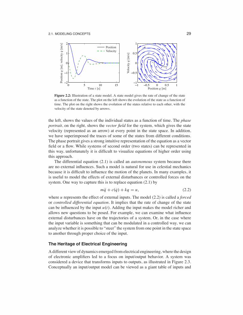
This system is illustrated in Figure 2.1. The variable q ! R represents the positionof the mass m with respect to its rest position. We use the notation q to denote thederivative of q with respect to time (i.e., the velocity of the mass) and q to representthe second derivative (acceleration). The spring is assumed to satisfy Hooke’s law,which says that the force is proportional to the displacement. The friction element(damper) is taken as a nonlinear function c(q), which can model effects such asstiction and viscous drag. The position q and velocity q represent the instantaneousstate of the system. We say that this system is a second-order system since thedynamics depend on the first two derivatives of q.The evolution of the position and velocity can be described using either a time
plot or a phase portrait, both of which are shown in Figure 2.2. The time plot, on
2.1. MODELING CONCEPTS 29
0 5 10 15−2
−1
0
1
2
Time t [s]
Positionq[m],velocityq[m/s] Position
Velocity
−1 −0.5 0 0.5 1−1
−0.5
0
0.5
1
Position q [m]
Velocityq[m/s]
Figure 2.2: Illustration of a state model. A state model gives the rate of change of the stateas a function of the state. The plot on the left shows the evolution of the state as a function oftime. The plot on the right shows the evolution of the states relative to each other, with thevelocity of the state denoted by arrows.
the left, shows the values of the individual states as a function of time. The phaseportrait, on the right, shows the vector field for the system, which gives the statevelocity (represented as an arrow) at every point in the state space. In addition,we have superimposed the traces of some of the states from different conditions.The phase portrait gives a strong intuitive representation of the equation as a vectorfield or a flow. While systems of second order (two states) can be represented inthis way, unfortunately it is difficult to visualize equations of higher order usingthis approach.The differential equation (2.1) is called an autonomous system because there
are no external influences. Such a model is natural for use in celestial mechanicsbecause it is difficult to influence the motion of the planets. In many examples, itis useful to model the effects of external disturbances or controlled forces on thesystem. One way to capture this is to replace equation (2.1) by
mq + c(q) + kq = u, (2.2)
where u represents the effect of external inputs. The model (2.2) is called a forcedor controlled differential equation. It implies that the rate of change of the statecan be influenced by the input u(t). Adding the input makes the model richer andallows new questions to be posed. For example, we can examine what influenceexternal disturbances have on the trajectories of a system. Or, in the case wherethe input variable is something that can be modulated in a controlled way, we cananalyze whether it is possible to “steer” the system from one point in the state spaceto another through proper choice of the input.
The Heritage of Electrical EngineeringAdifferent viewof dynamics emerged fromelectrical engineering,where the designof electronic amplifiers led to a focus on input/output behavior. A system wasconsidered a device that transforms inputs to outputs, as illustrated in Figure 2.3.Conceptually an input/output model can be viewed as a giant table of inputs and

30 CHAPTER 2. SYSTEM MODELING
7+v
–v
vos adj
(+)
(–)
InputsOutput3
2
6
4
Q9
Q1 Q2
Q3 Q4
Q7
Q5
R1 R12
R8
R7 R9
R10
R11R2
Q6Q22
Q17
Q16
Q1830pF
Q15
Q14
Q20
Q8
SystemInput Output
Figure 2.3: Illustration of the input/output view of a dynamical system. The figure on theleft shows a detailed circuit diagram for an electronic amplifier; the one on the right is itsrepresentation as a block diagram.
outputs. Given an input signal u(t) over some interval of time, the model shouldproduce the resulting output y(t).The input/output framework is used in many engineering disciplines since it
allows us to decompose a system into individual components connected throughtheir inputs and outputs. Thus, we can take a complicated system such as a radioor a television and break it down into manageable pieces such as the receiver,demodulator, amplifier and speakers. Each of these pieces has a set of inputs andoutputs and, through proper design, these components can be interconnected toform the entire system.The input/output view is particularly useful for the special class of linear time-
invariant systems. This term will be defined more carefully later in this chapter, butroughly speaking a system is linear if the superposition (addition) of two inputsyields an output that is the sum of the outputs that would correspond to individualinputs being applied separately. A system is time-invariant if the output responsefor a given input does not depend on when that input is applied.Many electrical engineering systems can be modeled by linear time-invariant
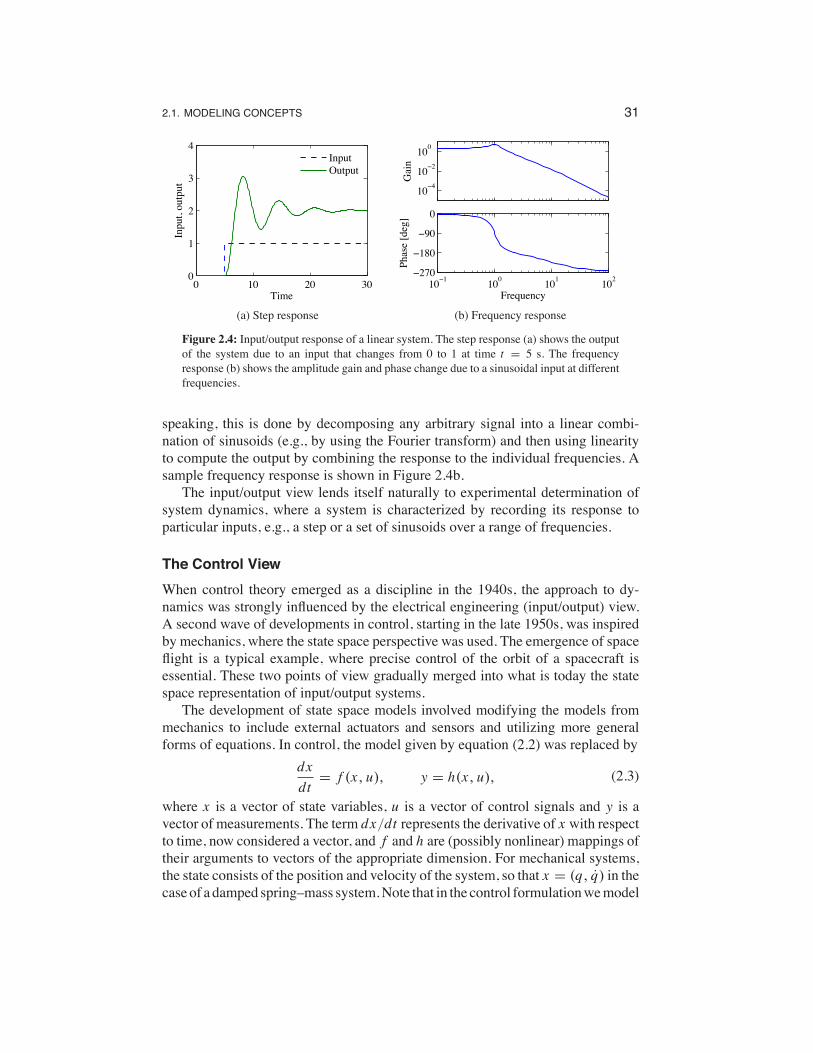
systems, and hence a large number of tools have been developed to analyze them.One such tool is the step response, which describes the relationship between aninput that changes from zero to a constant value abruptly (a step input) and thecorresponding output. As we shall see later in the text, the step response is veryuseful in characterizing the performance of a dynamical system, and it is often usedto specify the desired dynamics. A sample step response is shown in Figure 2.4a.Another way to describe a linear time-invariant system is to represent it by its
response to sinusoidal input signals. This is called the frequency response, and arich, powerful theory with many concepts and strong, useful results has emerged.The results are based on the theory of complex variables and Laplace transforms.The basic idea behind frequency response is that we can completely characterizethe behavior of a system by its steady-state response to sinusoidal inputs. Roughly
2.1. MODELING CONCEPTS 31
0 10 20 300
1
2
3
4
Time
Inpu
t, ou
tput
InputOutput
(a) Step response
10−4
10−2
100
Gai
n
10−1 100 101 102−270
−180
−90
0
Phas
e [d
eg]
Frequency
(b) Frequency response
Figure 2.4: Input/output response of a linear system. The step response (a) shows the outputof the system due to an input that changes from 0 to 1 at time t = 5 s. The frequencyresponse (b) shows the amplitude gain and phase change due to a sinusoidal input at differentfrequencies.
speaking, this is done by decomposing any arbitrary signal into a linear combi-nation of sinusoids (e.g., by using the Fourier transform) and then using linearityto compute the output by combining the response to the individual frequencies. Asample frequency response is shown in Figure 2.4b.The input/output view lends itself naturally to experimental determination of
system dynamics, where a system is characterized by recording its response toparticular inputs, e.g., a step or a set of sinusoids over a range of frequencies.
The Control ViewWhen control theory emerged as a discipline in the 1940s, the approach to dy-namics was strongly influenced by the electrical engineering (input/output) view.A second wave of developments in control, starting in the late 1950s, was inspiredby mechanics, where the state space perspective was used. The emergence of spaceflight is a typical example, where precise control of the orbit of a spacecraft isessential. These two points of view gradually merged into what is today the statespace representation of input/output systems.The development of state space models involved modifying the models from
mechanics to include external actuators and sensors and utilizing more generalforms of equations. In control, the model given by equation (2.2) was replaced by
dxdt
= f (x, u), y = h(x, u), (2.3)
where x is a vector of state variables, u is a vector of control signals and y is avector of measurements. The term dx/dt represents the derivative of x with respectto time, now considered a vector, and f and h are (possibly nonlinear) mappings oftheir arguments to vectors of the appropriate dimension. For mechanical systems,the state consists of the position and velocity of the system, so that x = (q, q) in thecase of a damped spring–mass system.Note that in the control formulationwemodel

32 CHAPTER 2. SYSTEM MODELING
dynamics as first-order differential equations, but we will see that this can capturethe dynamics of higher-order differential equations by appropriate definition of thestate and the maps f and h.Adding inputs and outputs has increased the richness of the classical problems
and led to many new concepts. For example, it is natural to ask if possible states xcan be reached with the proper choice of u (reachability) and if the measurement ycontains enough information to reconstruct the state (observability). These topicswill be addressed in greater detail in Chapters 6 and 7.A final development in building the control point of view was the emergence of
disturbances and model uncertainty as critical elements in the theory. The simpleway of modeling disturbances as deterministic signals like steps and sinusoids hasthe drawback that such signals cannot be predicted precisely. A more realistic ap-proach is to model disturbances as random signals. This viewpoint gives a naturalconnection between prediction and control. The dual views of input/output repre-sentations and state space representations are particularly useful when modelinguncertainty since state models are convenient to describe a nominal model but un-certainties are easier to describe using input/output models (often via a frequencyresponse description). Uncertainty will be a constant theme throughout the text andwill be studied in particular detail in Chapter 12.An interesting observation in the design of control systems is that feedback
systems can often be analyzed and designed based on comparatively simplemodels.The reason for this is the inherent robustness of feedback systems. However, otheruses of models may require more complexity and more accuracy. One example isfeedforward control strategies, where one uses a model to precompute the inputsthat cause the system to respond in a certain way. Another area is system validation,where one wishes to verify that the detailed response of the system performs as itwas designed. Because of these different uses of models, it is common to use ahierarchy of models having different complexity and fidelity.
Multidomain Modeling!
Modeling is an essential element of many disciplines, but traditions and methodsfrom individual disciplines can differ from each other, as illustrated by the previousdiscussion of mechanical and electrical engineering. A difficulty in systems engi-neering is that it is frequently necessary to deal with heterogeneous systems frommany different domains, including chemical, electrical, mechanical and informa-tion systems.To model such multidomain systems, we start by partitioning a system into
smaller subsystems. Each subsystem is represented by balance equations for mass,energy and momentum, or by appropriate descriptions of information processingin the subsystem. The behavior at the interfaces is captured by describing how thevariables of the subsystem behave when the subsystems are interconnected. Theseinterfaces act by constraining variables within the individual subsystems to be equal(such as mass, energy or momentum fluxes). The complete model is then obtainedby combining the descriptions of the subsystems and the interfaces.
2.1. MODELING CONCEPTS 33
Using this methodology it is possible to build up libraries of subsystems thatcorrespond to physical, chemical and informational components. The proceduremimics the engineering approach where systems are built from subsystems that arethemselves built fromsmaller components.As experience is gained, the componentsand their interfaces can be standardized and collected inmodel libraries. In practice,it takes several iterations to obtain a good library that can be reused for manyapplications.State models or ordinary differential equations are not suitable for component-
based modeling of this form because states may disappear when components areconnected. This implies that the internal description of a component may changewhen it is connected to other components. As an illustration we consider two ca-pacitors in an electrical circuit. Each capacitor has a state corresponding to thevoltage across the capacitors, but one of the states will disappear if the capacitorsare connected in parallel. A similar situation happens with two rotating inertias,each of which is individually modeled using the angle of rotation and the angularvelocity. Two states will disappear when the inertias are joined by a rigid shaft.This difficulty can be avoided by replacing differential equations by differential
algebraic equations, which have the form
F(z, z) = 0,
where z ! Rn . A simple special case is
x = f (x, y), g(x, y) = 0, (2.4)
where z = (x, y) and F = (x " f (x, y), g(x, y)). The key property is that thederivative z is not given explicitly and theremay be pure algebraic relations betweenthe components of the vector z.The model (2.4) captures the examples of the parallel capacitors and the linked
rotating inertias. For example, when two capacitors are connected, we simply addthe algebraic equation expressing that the voltages across the capacitors are thesame.
Modelica is a language that has been developed to support component-basedmodeling. Differential algebraic equations are used as the basic description, andobject-oriented programming is used to structure the models. Modelica is used tomodel the dynamics of technical systems in domains such as mechanical, electri-cal, thermal, hydraulic, thermofluid and control subsystems. Modelica is intendedto serve as a standard format so that models arising in different domains can beexchanged between tools and users. A large set of free and commercial Modelicacomponent libraries are available and are used by a growing number of peoplein industry, research and academia. For further information about Modelica, seehttp://www.modelica.org or Tiller [Til01].

34 CHAPTER 2. SYSTEM MODELING
2.2 State Space ModelsIn this section we introduce the two primary forms of models that we use in thistext: differential equations and difference equations. Both make use of the notionsof state, inputs, outputs and dynamics to describe the behavior of a system.
Ordinary Differential EquationsThe state of a system is a collection of variables that summarize the past of asystem for the purpose of predicting the future. For a physical system the state iscomposed of the variables required to account for storage of mass, momentum andenergy. A key issue in modeling is to decide how accurately this storage has to berepresented. The state variables are gathered in a vector x ! Rn called the statevector. The control variables are represented by another vector u ! Rp, and themeasured signal by the vector y ! Rq . A system can then be represented by thedifferential equation
dxdt
= f (x, u), y = h(x, u), (2.5)
where f : Rn # Rp $ Rn and h : Rn # Rp $ Rq are smooth mappings. We calla model of this form a state space model.The dimension of the state vector is called the order of the system. The sys-
tem (2.5) is called time-invariant because the functions f and h do not dependexplicitly on time t ; there are more general time-varying systems where the func-tions do depend on time. The model consists of two functions: the function f givesthe rate of change of the state vector as a function of state x and control u, and thefunction h gives the measured values as functions of state x and control u.A system is called a linear state space system if the functions f and h are linear
in x and u. A linear state space system can thus be represented bydxdt
= Ax + Bu, y = Cx + Du, (2.6)
where A, B, C and D are constant matrices. Such a system is said to be linear andtime-invariant, or LTI for short. The matrix A is called the dynamics matrix, thematrix B is called the control matrix, the matrix C is called the sensor matrix andthe matrix D is called the direct term. Frequently systems will not have a directterm, indicating that the control signal does not influence the output directly.A different form of linear differential equations, generalizing the second-order
dynamics from mechanics, is an equation of the form
dn ydtn
+ a1dn"1ydtn"1
+ · · · + an y = u, (2.7)
where t is the independent (time) variable, y(t) is the dependent (output) variableand u(t) is the input. The notation dk y/dtk is used to denote the kth derivativeof y with respect to t , sometimes also written as y(k). The controlled differentialequation (2.7) is said to be an nth-order system. This system can be converted into
2.2. STATE SPACE MODELS 35
state space form by defining
x =
!""""""""""""""""#
x1x2...
xn"1xn
$""""""""""""""""%
=
!""""""""""""""""#
dn"1y/dtn"1
dn"2y/dtn"2...
dy/dty
$""""""""""""""""%
,
and the state space equations become
ddt
!"""""""""""""""#
x1x2...
xn"1xn
$"""""""""""""""%
=
!"""""""""""""""#
"a1x1 " · · · " anxnx1...
xn"2xn"1
$"""""""""""""""%
+
!"""""""""""""""#
u0...00
$"""""""""""""""%
, y = xn.
With the appropriate definitions of A, B, C and D, this equation is in linear statespace form.An even more general system is obtained by letting the output be a linear com-
bination of the states of the system, i.e.,
y = b1x1 + b2x2 + · · · + bnxn + du.
This system can be modeled in state space as
ddt
!"""""""""""""""#
x1x2x3...xn
$"""""""""""""""%
=
!"""""""""""""""#
"a1 "a2 . . . "an"1 "an1 0 . . . 0 00 1 0 0...
. . ....
0 0 1 0
$"""""""""""""""%
x +
!"""""""""""""""#
100...0
$"""""""""""""""%
u,
y =!#b1 b2 . . . bn
$% x + du.
(2.8)
This particular form of a linear state space system is called reachable canonicalform and will be studied in more detail in later chapters.
Example 2.1 Balance systemsAn example of a type of system that can be modeled using ordinary differentialequations is the class of balance systems. A balance system is a mechanical systeminwhich the center ofmass is balanced above a pivot point. Some common examplesof balance systems are shown in Figure 2.5. The Segway® Personal Transporter(Figure 2.5a) uses a motorized platform to stabilize a person standing on top ofit. When the rider leans forward, the transportation device propels itself along theground butmaintains its upright position.Another example is a rocket (Figure 2.5b),in which a gimbaled nozzle at the bottom of the rocket is used to stabilize the bodyof the rocket above it. Other examples of balance systems include humans or otheranimals standing upright or a person balancing a stick on their hand.

36 CHAPTER 2. SYSTEM MODELING
(a) Segway (b) Saturn rocket
MF
p
!m
l
(c) Cart–pendulum system
Figure 2.5: Balance systems. (a) Segway Personal Transporter, (b) Saturn rocket and (c)inverted pendulum on a cart. Each of these examples uses forces at the bottom of the systemto keep it upright.
Balance systems are a generalization of the spring–mass system we saw earlier.We can write the dynamics for a mechanical system in the general form
M(q)q + C(q, q) + K (q) = B(q)u,
where M(q) is the inertia matrix for the system, C(q, q) represents the Coriolisforces as well as the damping, K (q) gives the forces due to potential energy andB(q) describes how the external applied forces couple into the dynamics. Thespecific form of the equations can be derived using Newtonian mechanics. Notethat each of the terms depends on the configuration of the system q and that theseterms are often nonlinear in the configuration variables.Figure 2.5c shows a simplified diagram for a balance system consisting of an
inverted pendulum on a cart. To model this system, we choose state variables thatrepresent the position and velocity of the base of the system, p and p, and the angleand angular rate of the structure above the base, ! and ! . We let F represent theforce applied at the base of the system, assumed to be in the horizontal direction(aligned with p), and choose the position and angle of the system as outputs. Withthis set of definitions, the dynamics of the system can be computed usingNewtonianmechanics and have the form
!""# (M + m) "ml cos !
"ml cos ! (J + ml2)
$""%
!""#p!
$""% +
!""#c p + ml sin ! !2
" ! " mgl sin !
$""% =
!""#F0
$""% , (2.9)
where M is the mass of the base,m and J are the mass and moment of inertia of thesystem to be balanced, l is the distance from the base to the center of mass of thebalanced body, c and " are coefficients of viscous friction and g is the accelerationdue to gravity.We can rewrite the dynamics of the system in state space form by defining the
state as x = (p, !, p, !), the input as u = F and the output as y = (p, !). If we

2.2. STATE SPACE MODELS 37
define the total mass and total inertia as
Mt = M + m, Jt = J + ml2,
the equations of motion then become
ddt
!"""""""""#
p!p!
$"""""""""%
=
!"""""""""""""""""""#
p!
"mls! !2 + mg(ml2/Jt)s!c! " c p " (" /Jt)mlc! ! + uMt " m(ml2/Jt)c2!
"ml2s!c! !2 + Mtgls! " clc! p " " (Mt/m)! + lc!u
Jt(Mt/m) " m(lc! )2
$"""""""""""""""""""%
,
y =!""#p
!
$""% ,
where we have used the shorthand c! = cos ! and s! = sin ! .In many cases, the angle ! will be very close to 0, and hence we can use the
approximations sin ! % ! and cos ! % 1. Furthermore, if ! is small, we canignore quadratic and higher terms in ! . Substituting these approximations into ourequations, we see that we are left with a linear state space equation
ddt
!"""""""""#
p!p!
$"""""""""%
=
!""""""""""#
0 0 1 00 0 0 10 m2l2g/µ "cJt/µ "" lm/µ
0 Mtmgl/µ "clm/µ ""Mt/µ
$""""""""""%
!"""""""""#
p!p!
$"""""""""%
+
!""""""""""#
00
Jt/µlm/µ
$""""""""""%u,
y =!""#1 0 0 00 1 0 0
$""% x,
where µ = Mt Jt " m2l2. &
Example 2.2 Inverted pendulumA variation of the previous example is one in which the location of the base p doesnot need to be controlled. This happens, for example, if we are interested only instabilizing a rocket’s upright orientation without worrying about the location ofbase of the rocket. The dynamics of this simplified system are given by
ddt
!""#
!!
$""% =
!"""""#
!mglJtsin ! "
"
Jt! +
lJtcos ! u
$"""""% , y = !, (2.10)
where " is the coefficient of rotational friction, Jt = J + ml2 and u is the forceapplied at the base. This system is referred to as an inverted pendulum. &
Difference EquationsIn some circumstances, it is more natural to describe the evolution of a system atdiscrete instants of time rather than continuously in time. If we refer to each of

38 CHAPTER 2. SYSTEM MODELING
these times by an integer k = 0, 1, 2, . . . , then we can ask how the state of thesystem changes for each k. Just as in the case of differential equations, we definethe state to be those sets of variables that summarize the past of the system for thepurpose of predicting its future. Systems described in this manner are referred toas discrete-time systems.The evolution of a discrete-time system can be written in the form
x[k + 1] = f (x[k], u[k]), y[k] = h(x[k], u[k]), (2.11)
where x[k] ! Rn is the state of the system at time k (an integer), u[k] ! Rp isthe input and y[k] ! Rq is the output. As before, f and h are smooth mappings ofthe appropriate dimension. We call equation (2.11) a difference equation since ittells us how x[k + 1] differs from x[k]. The state x[k] can be either a scalar- or avector-valued quantity; in the case of the latter we write x j [k] for the value of thej th state at time k.Just as in the case of differential equations, it is often the case that the equations
are linear in the state and input, in which case we can describe the system by
x[k + 1] = Ax[k]+ Bu[k], y[k] = Cx[k]+ Du[k].
Asbefore,we refer to thematrices A, B,C and D as the dynamicsmatrix, the controlmatrix, the sensor matrix and the direct term. The solution of a linear differenceequation with initial condition x[0] and input u[0], . . . , u[T ] is given by
x[k] = Akx0 +k"1&
j=0
Ak" j"1Bu[ j],
y[k] = CAkx0 +k"1&
j=0
CAk" j"1Bu[ j]+ Du[k],
k > 0. (2.12)
Difference equations are also useful as an approximation of differential equa-tions, as we will show later.
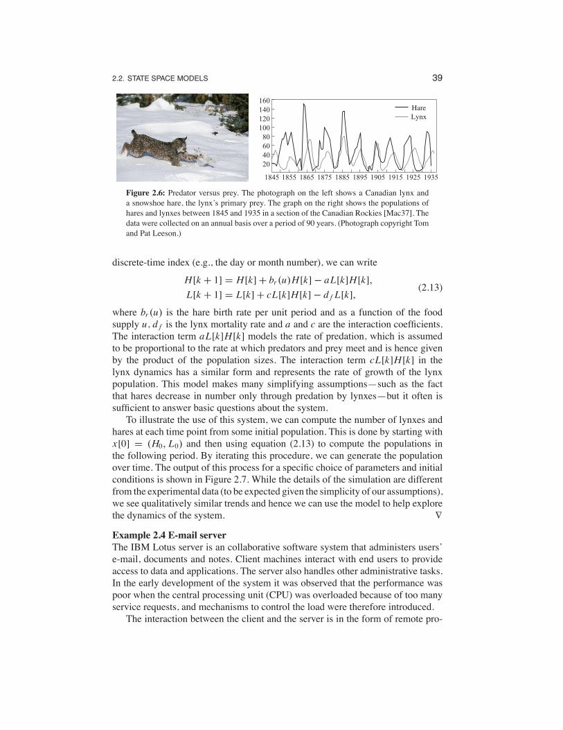
Example 2.3 Predator–preyAs an example of a discrete-time system, consider a simple model for a predator–prey system. The predator–prey problem refers to an ecological system in whichwe have two species, one of which feeds on the other. This type of system hasbeen studied for decades and is known to exhibit interesting dynamics. Figure 2.6shows a historical record taken over 90 years for a population of lynxes versus apopulation of hares [Mac37]. As can been seen from the graph, the annual recordsof the populations of each species are oscillatory in nature.A simplemodel for this situation can be constructed using a discrete-timemodel
by keeping track of the rate of births and deaths of each species. Letting H representthe population of hares and L represent the population of lynxes, we can describethe state in terms of the populations at discrete periods of time. Letting k be the
2.2. STATE SPACE MODELS 39
1845
160
140
120
100
80
60
40
20
1855 1865 1875 1885 1895
HareLynx
1905 1915 1925 1935
Figure 2.6: Predator versus prey. The photograph on the left shows a Canadian lynx anda snowshoe hare, the lynx’s primary prey. The graph on the right shows the populations ofhares and lynxes between 1845 and 1935 in a section of the Canadian Rockies [Mac37]. Thedata were collected on an annual basis over a period of 90 years. (Photograph copyright Tomand Pat Leeson.)
discrete-time index (e.g., the day or month number), we can write
H [k + 1] = H [k]+ br (u)H [k]" aL[k]H [k],L[k + 1] = L[k]+ cL[k]H [k]" d f L[k],
(2.13)
where br (u) is the hare birth rate per unit period and as a function of the foodsupply u, d f is the lynx mortality rate and a and c are the interaction coefficients.The interaction term aL[k]H [k] models the rate of predation, which is assumedto be proportional to the rate at which predators and prey meet and is hence givenby the product of the population sizes. The interaction term cL[k]H [k] in thelynx dynamics has a similar form and represents the rate of growth of the lynxpopulation. This model makes many simplifying assumptions—such as the factthat hares decrease in number only through predation by lynxes—but it often issufficient to answer basic questions about the system.To illustrate the use of this system, we can compute the number of lynxes and
hares at each time point from some initial population. This is done by starting withx[0] = (H0, L0) and then using equation (2.13) to compute the populations inthe following period. By iterating this procedure, we can generate the populationover time. The output of this process for a specific choice of parameters and initialconditions is shown in Figure 2.7. While the details of the simulation are differentfrom the experimental data (to be expected given the simplicity of our assumptions),we see qualitatively similar trends and hence we can use the model to help explorethe dynamics of the system. &
Example 2.4 E-mail serverThe IBM Lotus server is an collaborative software system that administers users’e-mail, documents and notes. Client machines interact with end users to provideaccess to data and applications. The server also handles other administrative tasks.In the early development of the system it was observed that the performance waspoor when the central processing unit (CPU) was overloaded because of too manyservice requests, and mechanisms to control the load were therefore introduced.The interaction between the client and the server is in the form of remote pro-

40 CHAPTER 2. SYSTEM MODELING
1850 1860 1870 1880 1890 1900 1910 19200
50
100
150
200
250
Year
Population
Hares Lynxes
Figure 2.7:Discrete-time simulation of the predator–preymodel (2.13). Using the parametersa = c = 0.014, br (u) = 0.6 and d = 0.7 in equation (2.13) with daily updates, the period andmagnitude of the lynx and hare population cycles approximately match the data in Figure 2.6.
cedure calls (RPCs). The server maintains a log of statistics of completed requests.The total number of requests being served, called RIS (RPCs in server), is alsomeasured. The load on the server is controlled by a parameter called MaxUsers,which sets the total number of client connections to the server. This parameter iscontrolled by the system administrator. The server can be regarded as a dynami-cal system with MaxUsers as the input and RIS as the output. The relationshipbetween input and output was first investigated by exploring the steady-state per-formance and was found to be linear.In [HDPT04] a dynamic model in the form of a first-order difference equation
is used to capture the dynamic behavior of this system. Using system identificationtechniques, they construct a model of the form
y[k + 1] = ay[k]+ bu[k],
where u = MaxUsers " MaxUsers and y = RIS " RIS. The parametersa = 0.43 and b = 0.47 are parameters that describe the dynamics of the systemaround the operating point, and MaxUsers = 165 and RIS = 135 represent thenominal operating point of the system. The number of requests was averaged overa sampling period of 60 s. &
Simulation and AnalysisState spacemodels can be used to answermany questions.One of themost common,as we have seen in the previous examples, involves predicting the evolution of thesystem state from a given initial condition. While for simple models this can bedone in closed form, more often it is accomplished through computer simulation.One can also use state space models to analyze the overall behavior of the systemwithout making direct use of simulation.Consider again the damped spring–mass system from Section 2.1, but this time
with an external force applied, as shown in Figure 2.8. We wish to predict themotion of the system for a periodic forcing function, with a given initial condition,and determine the amplitude, frequency and decay rate of the resulting motion.

2.2. STATE SPACE MODELS 41
q
m
k
u(t) = A sin t"
c
Figure 2.8: A driven spring–mass system with damping. Here we use a linear dampingelement with coefficient of viscous friction c. The mass is driven with a sinusoidal force ofamplitude A.
We choose to model the system with a linear ordinary differential equation.Using Hooke’s law to model the spring and assuming that the damper exerts a forcethat is proportional to the velocity of the system, we have
mq + cq + kq = u, (2.14)
where m is the mass, q is the displacement of the mass, c is the coefficient ofviscous friction, k is the spring constant and u is the applied force. In state spaceform, using x = (q, q) as the state and choosing y = q as the output, we have
dxdt
=
!""""""#
x2
"cmx2 "
kmx1 +
um
$""""""% , y = x1.
We see that this is a linear second-order differential equation with one input u andone output y.We now wish to compute the response of the system to an input of the form
u = A sin#t . Although it is possible to solve for the response analytically, weinstead make use of a computational approach that does not rely on the specificform of this system. Consider the general state space system
dxdt
= f (x, u).
Given the state x at time t , we can approximate the value of the state at a shorttime h > 0 later by assuming that the rate of change of f (x, u) is constant over theinterval t to t + h. This gives
x(t + h) = x(t) + h f (x(t), u(t)). (2.15)
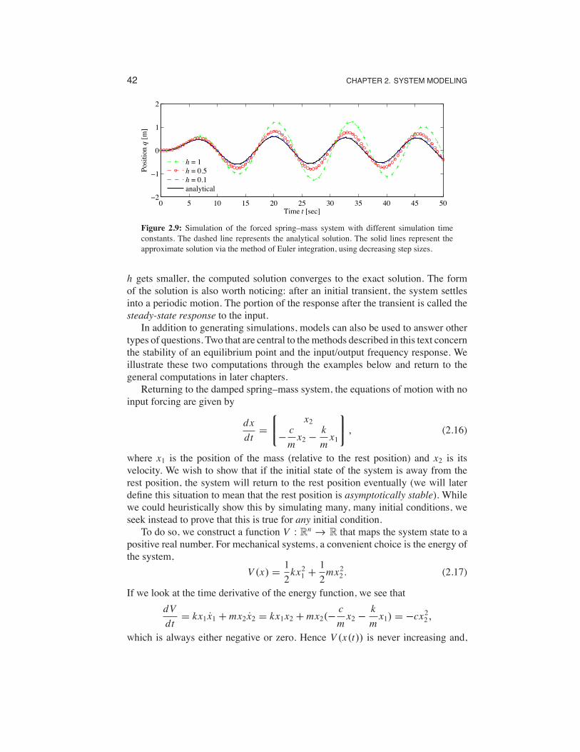
Iterating this equation, we can thus solve for x as a function of time. This approxi-mation is known as Euler integration and is in fact a difference equation if we let hrepresent the time increment and write x[k] = x(kh). Although modern simulationtools such as MATLAB and Mathematica use more accurate methods than Eulerintegration, they still have some of the same basic trade-offs.Returning to our specific example, Figure 2.9 shows the results of computing
x(t) using equation (2.15), along with the analytical computation. We see that as
42 CHAPTER 2. SYSTEM MODELING
0 5 10 15 20 25 30 35 40 45 50−2
−1
0
1
2
Time t [sec]
Posit
ion q
[m]
h = 1h = 0.5h = 0.1analytical
Figure 2.9: Simulation of the forced spring–mass system with different simulation timeconstants. The dashed line represents the analytical solution. The solid lines represent theapproximate solution via the method of Euler integration, using decreasing step sizes.
h gets smaller, the computed solution converges to the exact solution. The formof the solution is also worth noticing: after an initial transient, the system settlesinto a periodic motion. The portion of the response after the transient is called thesteady-state response to the input.In addition to generating simulations, models can also be used to answer other
types of questions. Two that are central to themethods described in this text concernthe stability of an equilibrium point and the input/output frequency response. Weillustrate these two computations through the examples below and return to thegeneral computations in later chapters.Returning to the damped spring–mass system, the equations of motion with no
input forcing are given by
dxdt
=
!""""#
x2"cmx2 "
kmx1
$""""% , (2.16)
where x1 is the position of the mass (relative to the rest position) and x2 is itsvelocity. We wish to show that if the initial state of the system is away from therest position, the system will return to the rest position eventually (we will laterdefine this situation to mean that the rest position is asymptotically stable). Whilewe could heuristically show this by simulating many, many initial conditions, weseek instead to prove that this is true for any initial condition.To do so, we construct a function V : Rn $ R that maps the system state to a
positive real number. For mechanical systems, a convenient choice is the energy ofthe system,
V (x) =12kx21 +
12mx22 . (2.17)
If we look at the time derivative of the energy function, we see thatdVdt
= kx1 x1 + mx2 x2 = kx1x2 + mx2("cmx2 "
kmx1) = "cx22 ,
which is always either negative or zero. Hence V (x(t)) is never increasing and,
2.2. STATE SPACE MODELS 43
using a bit of analysis that we will see formally later, the individual states mustremain bounded.If we wish to show that the states eventually return to the origin, we must use
a slightly more detailed analysis. Intuitively, we can reason as follows: supposethat for some period of time, V (x(t)) stops decreasing. Then it must be true thatV (x(t)) = 0, which in turn implies that x2(t) = 0 for that same period. In thatcase, x2(t) = 0, and we can substitute into the second line of equation (2.16) toobtain
0 = x2 = "cmx2 "
kmx1 =
kmx1.
Thus we must have that x1 also equals zero, and so the only time that V (x(t)) canstop decreasing is if the state is at the origin (and hence this system is at its restposition). Since we know that V (x(t)) is never increasing (because V ' 0), wetherefore conclude that the origin is stable (for any initial condition).This type of analysis, called Lyapunov stability analysis, is considered in detail
in Chapter 4. It shows some of the power of using models for the analysis of systemproperties.
Another type of analysis that we can perform with models is to compute theoutput of a system to a sinusoidal input.We again consider the spring–mass system,but this time keeping the input and leaving the system in its original form:
mq + cq + kq = u. (2.18)
We wish to understand how the system responds to a sinusoidal input of the form
u(t) = A sin#t.
We will see how to do this analytically in Chapter 6, but for now we make use ofsimulations to compute the answer.We first begin with the observation that if q(t) is the solution to equation (2.18)
with input u(t), then applying an input 2u(t)will give a solution 2q(t) (this is easilyverified by substitution). Hence it suffices to look at an input with unit magnitude,A = 1. A second observation, which we will prove in Chapter 5, is that the long-term response of the system to a sinusoidal input is itself a sinusoid at the samefrequency, and so the output has the form
q(t) = g(#) sin(#t + $(#)),
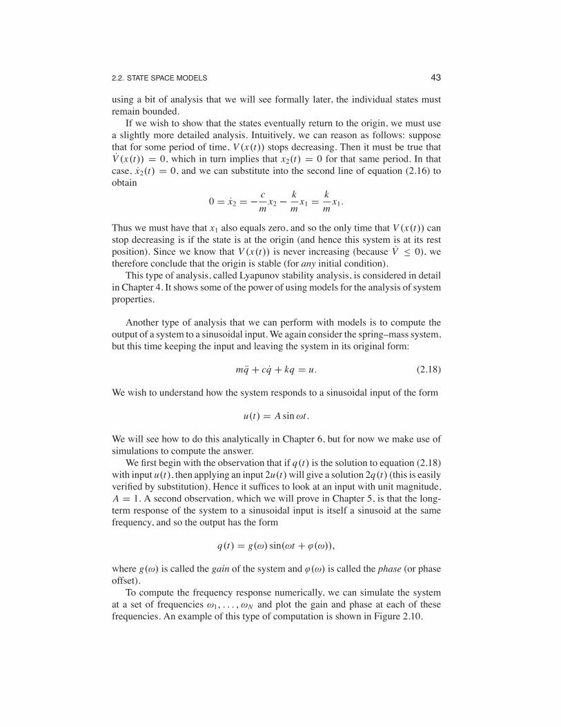
where g(#) is called the gain of the system and $(#) is called the phase (or phaseoffset).To compute the frequency response numerically, we can simulate the system
at a set of frequencies #1, . . . , #N and plot the gain and phase at each of thesefrequencies. An example of this type of computation is shown in Figure 2.10.
44 CHAPTER 2. SYSTEM MODELING
0 10 20 30 40 50−4
−2
0
2
4
Outputy
Time [s]10−1 100 101
10−2
10−1
100
101
Gain(logscale)
Frequency [rad/sec] (log scale)
Figure 2.10: A frequency response (gain only) computed by measuring the response ofindividual sinusoids. The figure on the left shows the response of the system as a function oftime to a number of different unit magnitude inputs (at different frequencies). The figure onthe right shows this same data in a different way, with the magnitude of the response plottedas a function of the input frequency. The filled circles correspond to the particular frequenciesshown in the time responses.
2.3 Modeling MethodologyTo deal with large, complex systems, it is useful to have different representationsof the system that capture the essential features and hide irrelevant details. In allbranches of science and engineering it is common practice to use some graphicaldescription of systems, called schematic diagrams. They can range from stylisticpictures to drastically simplified standard symbols. These pictures make it possibleto get an overall view of the system and to identify the individual components.Examples of such diagrams are shown inFigure 2.11. Schematic diagrams are usefulbecause they give an overall picture of a system, showing different subprocesses andtheir interconnection and indicating variables that can be manipulated and signalsthat can be measured.
Block DiagramsA special graphical representation called a block diagram has been developed incontrol engineering. The purpose of a block diagram is to emphasize the informationflow and to hide details of the system. In a block diagram, different process elementsare shown as boxes, and each box has inputs denoted by lines with arrows pointingtoward the box and outputs denoted by lines with arrows going out of the box.The inputs denote the variables that influence a process, and the outputs denotethe signals that we are interested in or signals that influence other subsystems.Block diagrams can also be organized in hierarchies, where individual blocks maythemselves contain more detailed block diagrams.Figure 2.12 shows some of the notation that we use for block diagrams. Signals
are represented as lines,with arrows to indicate inputs and outputs. The first diagramis the representation for a summation of two signals. An input/output response isrepresented as a rectangle with the system name (or mathematical description) in

2.3. MODELING METHODOLOGY 45
1
3
5
2
Buscoding
Bussymbol
Generatorsymbol
Transformersymbol
Tie lineconnecting withneighbor system
Line symbol
Load symbol
6
4
(a) Power electronics
–150
glnAp2 glnG
NRI NRI-P
glnKp lacl
Lacl
0° 0°
(b) Cell biology
LC
LC
AT
AC
D
B
V
L
AC
AT
(c) Process control
t5t6
t3
t4
t1
p1
(ready tosend)
(bufferin use)
(bufferin use)
(input)(output) (ready toreceive)
(consume)
(ack. sent)(receiveack.)
Process A Process B
(ack.received)
(produce)(received)
(sendack.)
(waitingfor ack.)
p3
p8
p6
p4p5
p2
p7
(d) Networking
Figure 2.11: Schematic diagrams for different disciplines. Each diagram is used to illustratethe dynamics of a feedback system: (a) electrical schematics for a power system [Kun93], (b)a biological circuit diagram for a synthetic clock circuit [ASMN03], (c) a process diagram fora distillation column [SEM04] and (d) a Petri net description of a communication protocol.
u1 u1 + u2u2
%
(a) Summing junction
kkuu
(b) Gain block
sat(u)u
(c) Saturation
u f (u)
(d) Nonlinear map
'u
' t
0u(t) dt
(e) Integrator
Systemu y
(f) Input/output system
Figure 2.12: Standard block diagram elements. The arrows indicate the the inputs and outputsof each element, with the mathematical operation corresponding to the blocked labeled at theoutput. The system block (f) represents the full input/output response of a dynamical system.
46 CHAPTER 2. SYSTEM MODELING
Wind
%%Ref (a) Sensory
MotorSystem
(b) WingAero-
dynamics
(c) BodyDynamics
(d) DragAero-
dynamics
(e) VisionSystem"1
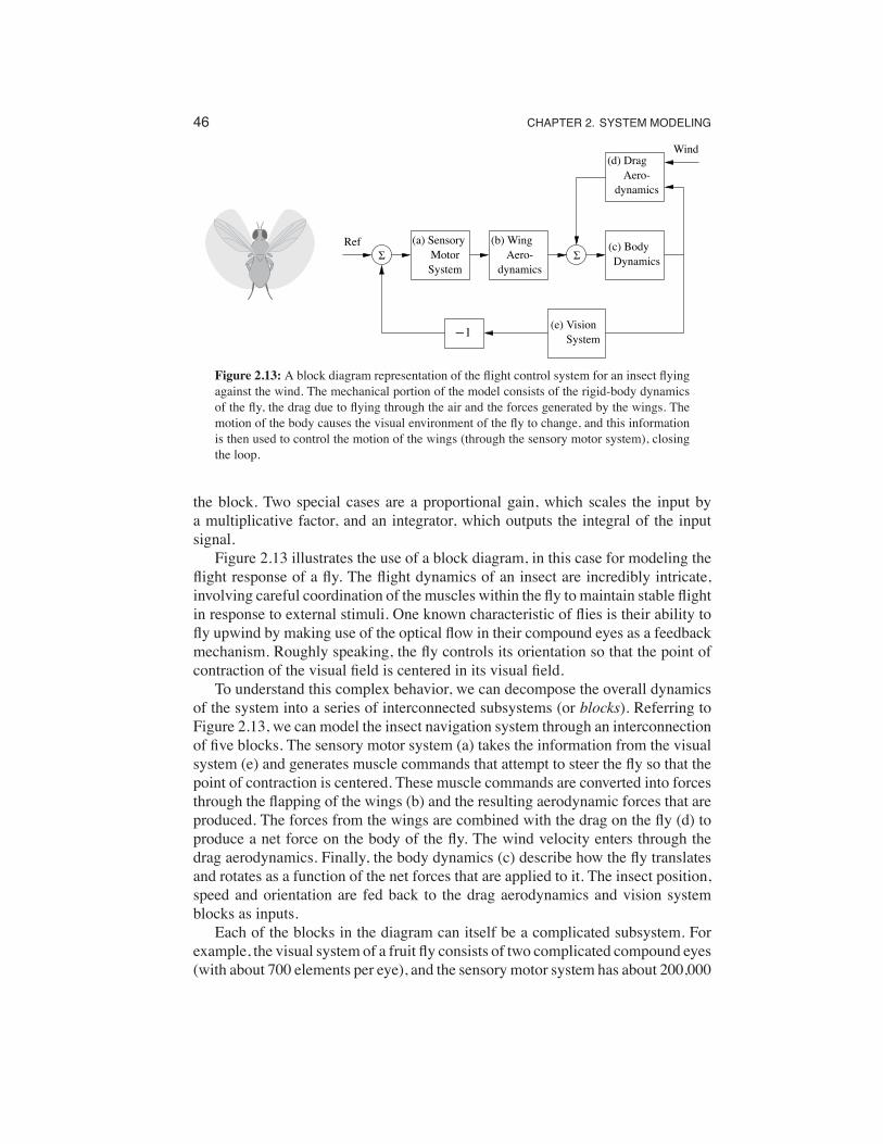
Figure 2.13: A block diagram representation of the flight control system for an insect flyingagainst the wind. The mechanical portion of the model consists of the rigid-body dynamicsof the fly, the drag due to flying through the air and the forces generated by the wings. Themotion of the body causes the visual environment of the fly to change, and this informationis then used to control the motion of the wings (through the sensory motor system), closingthe loop.
the block. Two special cases are a proportional gain, which scales the input bya multiplicative factor, and an integrator, which outputs the integral of the inputsignal.Figure 2.13 illustrates the use of a block diagram, in this case for modeling the
flight response of a fly. The flight dynamics of an insect are incredibly intricate,involving careful coordination of the muscles within the fly to maintain stable flightin response to external stimuli. One known characteristic of flies is their ability tofly upwind by making use of the optical flow in their compound eyes as a feedbackmechanism. Roughly speaking, the fly controls its orientation so that the point ofcontraction of the visual field is centered in its visual field.To understand this complex behavior, we can decompose the overall dynamics
of the system into a series of interconnected subsystems (or blocks). Referring toFigure 2.13, we can model the insect navigation system through an interconnectionof five blocks. The sensory motor system (a) takes the information from the visualsystem (e) and generates muscle commands that attempt to steer the fly so that thepoint of contraction is centered. These muscle commands are converted into forcesthrough the flapping of the wings (b) and the resulting aerodynamic forces that areproduced. The forces from the wings are combined with the drag on the fly (d) toproduce a net force on the body of the fly. The wind velocity enters through thedrag aerodynamics. Finally, the body dynamics (c) describe how the fly translatesand rotates as a function of the net forces that are applied to it. The insect position,speed and orientation are fed back to the drag aerodynamics and vision systemblocks as inputs.Each of the blocks in the diagram can itself be a complicated subsystem. For
example, the visual system of a fruit fly consists of two complicated compound eyes(with about 700 elements per eye), and the sensory motor system has about 200,000

2.3. MODELING METHODOLOGY 47
neurons that are used to process information. A more detailed block diagram ofthe insect flight control system would show the interconnections between theseelements, but here we have used one block to represent how the motion of the flyaffects the output of the visual system, and a secondblock to represent how the visualfield is processed by the fly’s brain to generate muscle commands. The choice of thelevel of detail of the blocks andwhat elements to separate into different blocks oftendepends on experience and the questions that one wants to answer using the model.One of the powerful features of block diagrams is their ability to hide informationabout the details of a system that may not be needed to gain an understanding ofthe essential dynamics of the system.
Modeling from ExperimentsSince control systems are provided with sensors and actuators, it is also possible toobtain models of system dynamics from experiments on the process. The modelsare restricted to input/output models since only these signals are accessible toexperiments, but modeling from experiments can also be combined with modelingfrom physics through the use of feedback and interconnection.A simple way to determine a system’s dynamics is to observe the response to a
step change in the control signal. Such an experiment begins by setting the controlsignal to a constant value; then when steady state is established, the control signal ischanged quickly to a new level and the output is observed. The experiment gives thestep response of the system, and the shape of the response gives useful informationabout the dynamics. It immediately gives an indication of the response time, and ittells if the system is oscillatory or if the response is monotone.
Example 2.5 Spring–mass systemConsider the spring–mass system from Section 2.1, whose dynamics are given by
mq + cq + kq = u. (2.19)
We wish to determine the constants m, c and k by measuring the response of thesystem to a step input of magnitude F0.We will show in Chapter 6 that when c2 < 4km, the step response for this
system from the rest configuration is given by
q(t) =F0k
(1" exp
)"ct2m
*sin(#d t + $)
+,
#d =(4km " c2
2m,
$ = tan"1,-4km " c2
..
From the form of the solution, we see that the form of the response is determinedby the parameters of the system. Hence, by measuring certain features of the stepresponse we can determine the parameter values.Figure 2.14 shows the response of the system to a step of magnitude F0 = 20
N, along with some measurements. We start by noting that the steady-state position

48 CHAPTER 2. SYSTEM MODELING
0 5 10 15 20 25 30 35 40 45 500
0.2
0.4
0.6
0.8
Time t [s]
Posit
ion q
[m]
q(t1)
q(t2) q(∞)
T
Figure 2.14: Step response for a spring–mass system. The magnitude of the step input isF0 = 20 N. The period of oscillation T is determined by looking at the time between twosubsequent local maxima in the response. The period combined with the steady-state valueq()) and the relative decrease between local maxima can be used to estimate the parametersin a model of the system.
of the mass (after the oscillations die down) is a function of the spring constant k:
q()) =F0k
, (2.20)
where F0 is the magnitude of the applied force (F0 = 1 for a unit step input). Theparameter 1/k is called the gain of the system. The period of the oscillation can bemeasured between two peaks and must satisfy
2&T
=(4km " c2
2m. (2.21)
Finally, the rate of decay of the oscillations is given by the exponential factor in thesolution. Measuring the amount of decay between two peaks, we have
log,q(t1) "
F0k
." log
,q(t2) "
F0k
.=
c2m
(t2 " t1). (2.22)
Using this set of three equations, we can solve for the parameters and determinethat for the step response in Figure 2.14 we have m % 250 kg, c % 60 N s/m andk % 40 N/m. &
Modeling from experiments can also be done using many other signals. Si-nusoidal signals are commonly used (particularly for systems with fast dynamics)and precise measurements can be obtained by exploiting correlation techniques. Anindication of nonlinearities can be obtained by repeating experiments with inputsignals having different amplitudes.
Normalization and ScalingHaving obtained a model, it is often useful to scale the variables by introducingdimension-free variables. Such a procedure can often simplify the equations for asystem by reducing the number of parameters and reveal interesting properties of

2.3. MODELING METHODOLOGY 49
the model. Scaling can also improve the numerical conditioning of the model toallow faster and more accurate simulations.The procedure of scaling is straightforward: choose units for each indepen-
dent variable and introduce new variables by dividing the variables by the chosennormalization unit. We illustrate the procedure with two examples.
Example 2.6 Spring–mass systemConsider again the spring–mass system introduced earlier. Neglecting the damping,the system is described by
mq + kq = u.
The model has two parameters m and k. To normalize the model we introducedimension-free variables x = q/ l and ' = #0t , where #0 =
(k/m and l is the
chosen length scale. We scale force by ml#20 and introduce v = u/(ml#20). Thescaled equation then becomes
d2xd' 2
=d2q/ ld(#0t)2
=1
ml#20("kq + u) = "x + v,
which is the normalized undamped spring–mass system. Notice that the normalizedmodel has no parameters, while the original model had two parameters m and k.Introducing the scaled, dimension-free state variables z1 = x = q/ l and z2 =dx/d' = q/(l#0), the model can be written as
ddt
!""#z1z2
$""% =
!""# 0 1
"1 0
$""%
!""#z1z2
$""% +
!""#0
v
$""% .
This simple linear equation describes the dynamics of any spring–mass system,independent of the particular parameters, and hence gives us insight into the fun-damental dynamics of this oscillatory system. To recover the physical frequency ofoscillation or its magnitude, we must invert the scaling we have applied. &
Example 2.7 Balance systemConsider the balance system described in Section 2.1. Neglecting damping byputting c = 0 and " = 0 in equation (2.9), the model can be written as
(M + m)d2qdt2
" ml cos !d2!dt2
+ ml sin !)dqdt
*2 = F,
"ml cos !d2qdt2
+ (J + ml2)d2!dt2
" mgl sin ! = 0.
Let#0 =-mgl/(J + ml2), choose the length scale as l, let the time scale be 1/#0,
choose the force scale as (M +m)l#20 and introduce the scaled variables ' = #0t ,x = q/ l and u = F/((M + m)l#20). The equations then become
d2xd' 2
" ( cos !d2!d' 2
+ ( sin !,d!
d'
.2= u, ") cos !
d2xd' 2
+d2!d' 2
" sin ! = 0,
where ( = m/(M+m) and ) = ml2/(J+ml2). Notice that the original model hasfive parametersm, M , J , l and g but the normalized model has only two parameters

50 CHAPTER 2. SYSTEM MODELING
10−2 100 102
10−2
100
102
Input u
Out
put y
(a) Static uncertainty
101 102 103
10−1
100
101
Frequency
Am
plitu
de
(b) Uncertainty lemon
*
%u y
M
(c) Model uncertainty
Figure 2.15: Characterization of model uncertainty. Uncertainty of a static system is illus-trated in (a), where the solid line indicates the nominal input/output relationship and thedashed lines indicate the range of possible uncertainty. The uncertainty lemon [GPD59] in(b) is one way to capture uncertainty in dynamical systems emphasizing that a model is validonly in some amplitude and frequency ranges. In (c) a model is represented by a nominalmodel M and another model * representing the uncertainty analogous to the representationof parameter uncertainty.
( and ). If M * m and ml2 * J , we get ( % 0 and ) % 1 and the model can beapproximated by
d2xd' 2
= u,d2!d' 2
" sin ! = u cos ! .
Themodel can be interpreted as amass combinedwith an inverted pendulum drivenby the same input. &
Model UncertaintyReducing uncertainty is one of the main reasons for using feedback, and it is there-fore important to characterize uncertainty. When making measurements, there is agood tradition to assign both a nominal value and a measure of uncertainty. It isuseful to apply the same principle to modeling, but unfortunately it is often difficultto express the uncertainty of a model quantitatively.For a static system whose input/output relation can be characterized by a func-
tion, uncertainty can be expressed by an uncertainty band as illustrated in Fig-ure 2.15a. At low signal levels there are uncertainties due to sensor resolution,friction and quantization. Some models for queuing systems or cells are based onaverages that exhibit significant variations for small populations. At large signallevels there are saturations or even system failures. The signal ranges where amodelis reasonably accurate vary dramatically between applications, but it is rare to findmodels that are accurate for signal ranges larger than 104.Characterization of the uncertainty of a dynamic model is much more difficult.
We can try to capture uncertainties by assigning uncertainties to parameters of themodel, but this is often not sufficient. There may be errors due to phenomena thathave been neglected, e.g., small time delays. In control the ultimate test is how wella control system based on the model performs, and time delays can be important.There is also a frequency aspect. There are slow phenomena, such as aging, that

2.4. MODELING EXAMPLES 51
can cause changes or drift in the systems. There are also high-frequency effects: aresistor will no longer be a pure resistance at very high frequencies, and a beamhas stiffness and will exhibit additional dynamics when subject to high-frequencyexcitation. The uncertainty lemon [GPD59] shown in Figure 2.15b is one way toconceptualize the uncertainty of a system. It illustrates that a model is valid only incertain amplitude and frequency ranges.We will introduce some formal tools for representing uncertainty in Chapter 12
using figures such as Figure 2.15c. These tools make use of the concept of a transferfunction, which describes the frequency response of an input/output system. Fornow, we simply note that one should always be careful to recognize the limits ofa model and not to make use of models outside their range of applicability. Forexample, one can describe the uncertainty lemon and then check to make sure thatsignals remain in this region. In early analog computing, a system was simulatedusing operational amplifiers, and it was customary to give alarms when certainsignal levels were exceeded. Similar features can be included in digital simulation.
2.4 Modeling ExamplesIn this section we introduce additional examples that illustrate some of the differenttypes of systems for which one can develop differential equation and differenceequation models. These examples are specifically chosen from a range of differentfields to highlight the broad variety of systems to which feedback and controlconcepts can be applied. A more detailed set of applications that serve as runningexamples throughout the text are given in the next chapter.
Motion Control SystemsMotion control systems involve the use of computation and feedback to control themovement of a mechanical system. Motion control systems range from nanopo-sitioning systems (atomic force microscopes, adaptive optics), to control systemsfor the read/write heads in a disk drive of a CD player, to manufacturing systems(transfer machines and industrial robots), to automotive control systems (antilockbrakes, suspension control, traction control), to air and space flight control systems(airplanes, satellites, rockets and planetary rovers).
Example 2.8 Vehicle steering—the bicycle modelA common problem in motion control is to control the trajectory of a vehiclethrough an actuator that causes a change in the orientation. A steering wheel on anautomobile and the front wheel of a bicycle are two examples, but similar dynamicsoccur in the steering of ships or control of the pitch dynamics of an aircraft. In manycases, we can understand the basic behavior of these systems through the use of asimple model that captures the basic kinematics of the system.Consider a vehicle with two wheels as shown in Figure 2.16. For the purpose of
steering we are interested in a model that describes how the velocity of the vehicle
52 CHAPTER 2. SYSTEM MODELING
ab
# $v
y
x
!
!
"
"
O
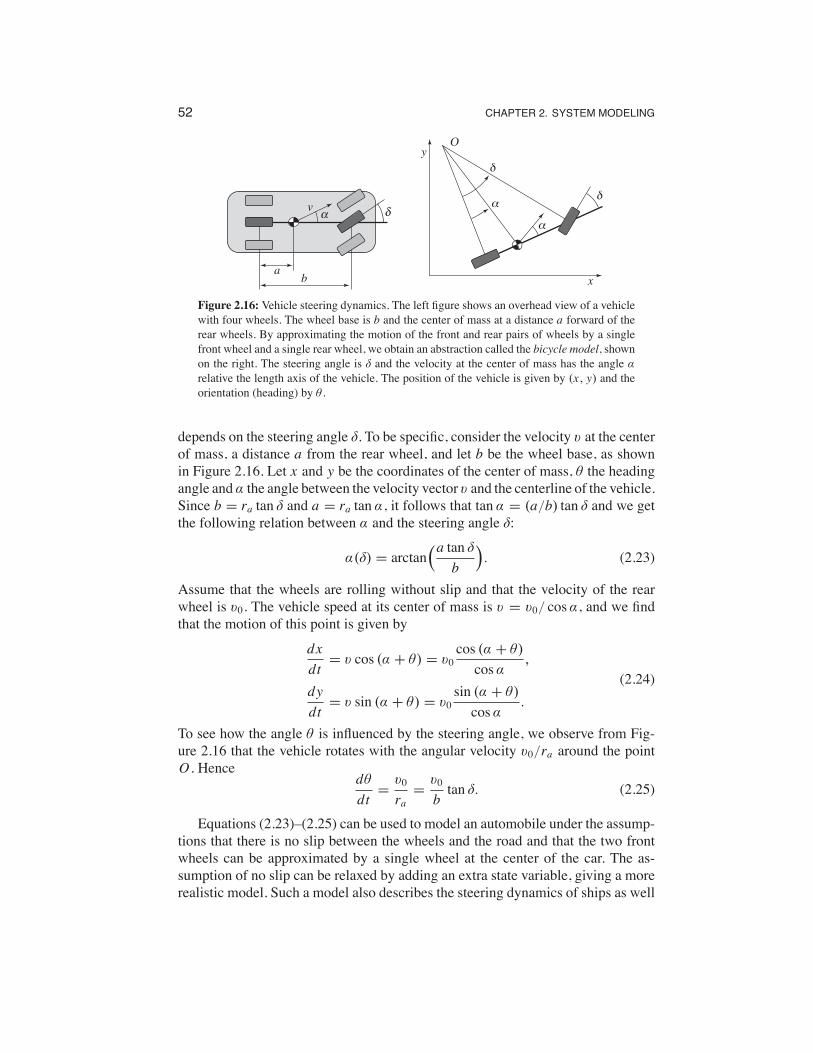
Figure 2.16: Vehicle steering dynamics. The left figure shows an overhead view of a vehiclewith four wheels. The wheel base is b and the center of mass at a distance a forward of therear wheels. By approximating the motion of the front and rear pairs of wheels by a singlefront wheel and a single rear wheel, we obtain an abstraction called the bicycle model, shownon the right. The steering angle is + and the velocity at the center of mass has the angle (relative the length axis of the vehicle. The position of the vehicle is given by (x, y) and theorientation (heading) by ! .
depends on the steering angle +. To be specific, consider the velocity v at the centerof mass, a distance a from the rear wheel, and let b be the wheel base, as shownin Figure 2.16. Let x and y be the coordinates of the center of mass, ! the headingangle and( the angle between the velocity vector v and the centerline of the vehicle.Since b = ra tan + and a = ra tan (, it follows that tan ( = (a/b) tan + and we getthe following relation between ( and the steering angle +:
((+) = arctan,a tan +
b
.. (2.23)
Assume that the wheels are rolling without slip and that the velocity of the rearwheel is v0. The vehicle speed at its center of mass is v = v0/ cos(, and we findthat the motion of this point is given by
dxdt
= v cos (( + !) = v0cos (( + !)
cos(,
dydt
= v sin (( + !) = v0sin (( + !)
cos(.
(2.24)
To see how the angle ! is influenced by the steering angle, we observe from Fig-ure 2.16 that the vehicle rotates with the angular velocity v0/ra around the pointO . Hence
d!
dt=
v0ra
=v0btan +. (2.25)
Equations (2.23)–(2.25) can be used to model an automobile under the assump-tions that there is no slip between the wheels and the road and that the two frontwheels can be approximated by a single wheel at the center of the car. The as-sumption of no slip can be relaxed by adding an extra state variable, giving a morerealistic model. Such a model also describes the steering dynamics of ships as well

2.4. MODELING EXAMPLES 53
(a) Harrier “jump jet”
r
x
y
!
F1
F2
(b) Simplified model
Figure 2.17: Vectored thrust aircraft. The Harrier AV-8B military aircraft (a) redirects itsengine thrust downward so that it can “hover” above the ground. Some air from the engineis diverted to the wing tips to be used for maneuvering. As shown in (b), the net thrust onthe aircraft can be decomposed into a horizontal force F1 and a vertical force F2 acting at adistance r from the center of mass.
as the pitch dynamics of aircraft and missiles. It is also possible to choose coor-dinates so that the reference point is at the rear wheels (corresponding to setting( = 0), a model often referred to as the Dubins car [Dub57].Figure 2.16 represents the situation when the vehicle moves forward and has
front-wheel steering. The case when the vehicle reverses is obtained by changingthe sign of the velocity, which is equivalent to a vehicle with rear-wheel steering.
&
Example 2.9 Vectored thrust aircraftConsider the motion of vectored thrust aircraft, such as the Harrier “jump jet”shown Figure 2.17a. The Harrier is capable of vertical takeoff by redirecting itsthrust downward and through the use of smaller maneuvering thrusters located onits wings. A simplified model of the Harrier is shown in Figure 2.17b, where wefocus on the motion of the vehicle in a vertical plane through the wings of theaircraft. We resolve the forces generated by the main downward thruster and themaneuvering thrusters as a pair of forces F1 and F2 acting at a distance r below theaircraft (determined by the geometry of the thrusters).Let (x, y, !) denote the position and orientation of the center of mass of the
aircraft. Letm be themass of the vehicle, J themoment of inertia, g the gravitationalconstant and c the damping coefficient. Then the equations ofmotion for the vehicleare given by
mx = F1 cos ! " F2 sin ! " cx,my = F1 sin ! + F2 cos ! " mg " cy,J ! = r F1.
(2.26)
It is convenient to redefine the inputs so that the origin is an equilibrium point of the
54 CHAPTER 2. SYSTEM MODELING
message queue
incoming outgoingmessages
x
µ,
messages
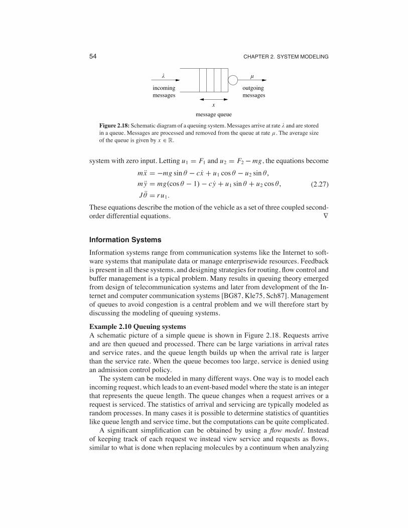
Figure 2.18: Schematic diagram of a queuing system.Messages arrive at rate , and are storedin a queue. Messages are processed and removed from the queue at rate µ. The average sizeof the queue is given by x ! R.
system with zero input. Letting u1 = F1 and u2 = F2 "mg, the equations becomemx = "mg sin ! " cx + u1 cos ! " u2 sin !,
my = mg(cos ! " 1) " cy + u1 sin ! + u2 cos !,
J ! = ru1.(2.27)
These equations describe the motion of the vehicle as a set of three coupled second-order differential equations. &
Information SystemsInformation systems range from communication systems like the Internet to soft-ware systems that manipulate data or manage enterprisewide resources. Feedbackis present in all these systems, and designing strategies for routing, flow control andbuffer management is a typical problem. Many results in queuing theory emergedfrom design of telecommunication systems and later from development of the In-ternet and computer communication systems [BG87, Kle75, Sch87]. Managementof queues to avoid congestion is a central problem and we will therefore start bydiscussing the modeling of queuing systems.
Example 2.10 Queuing systemsA schematic picture of a simple queue is shown in Figure 2.18. Requests arriveand are then queued and processed. There can be large variations in arrival ratesand service rates, and the queue length builds up when the arrival rate is largerthan the service rate. When the queue becomes too large, service is denied usingan admission control policy.The system can be modeled in many different ways. One way is to model each
incoming request, which leads to an event-based model where the state is an integerthat represents the queue length. The queue changes when a request arrives or arequest is serviced. The statistics of arrival and servicing are typically modeled asrandom processes. In many cases it is possible to determine statistics of quantitieslike queue length and service time, but the computations can be quite complicated.A significant simplification can be obtained by using a flow model. Instead
of keeping track of each request we instead view service and requests as flows,similar to what is done when replacing molecules by a continuum when analyzing
2.4. MODELING EXAMPLES 55
0 0.5 10
50
100
Service rate excess λ/µmax
Que
ue le
ngth
xe
(a) Steady-state queue size
0 20 40 60 800
10
20
Time [s]
Que
ue le
ngth
xe
(b) Overload condition
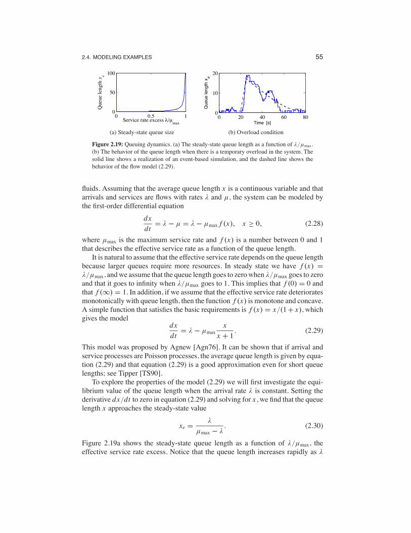
Figure 2.19: Queuing dynamics. (a) The steady-state queue length as a function of ,/µmax.(b) The behavior of the queue length when there is a temporary overload in the system. Thesolid line shows a realization of an event-based simulation, and the dashed line shows thebehavior of the flow model (2.29).
fluids. Assuming that the average queue length x is a continuous variable and thatarrivals and services are flows with rates , and µ, the system can be modeled bythe first-order differential equation
dxdt
= , " µ = , " µmax f (x), x + 0, (2.28)
where µmax is the maximum service rate and f (x) is a number between 0 and 1that describes the effective service rate as a function of the queue length.It is natural to assume that the effective service rate depends on the queue length
because larger queues require more resources. In steady state we have f (x) =,/µmax, andwe assume that the queue length goes to zerowhen ,/µmax goes to zeroand that it goes to infinity when ,/µmax goes to 1. This implies that f (0) = 0 andthat f ()) = 1. In addition, if we assume that the effective service rate deterioratesmonotonically with queue length, then the function f (x) is monotone and concave.A simple function that satisfies the basic requirements is f (x) = x/(1+ x), whichgives the model
dxdt
= , " µmaxx
x + 1. (2.29)
This model was proposed by Agnew [Agn76]. It can be shown that if arrival andservice processes are Poisson processes, the average queue length is given by equa-tion (2.29) and that equation (2.29) is a good approximation even for short queuelengths; see Tipper [TS90].To explore the properties of the model (2.29) we will first investigate the equi-
librium value of the queue length when the arrival rate , is constant. Setting thederivative dx/dt to zero in equation (2.29) and solving for x , we find that the queuelength x approaches the steady-state value
xe =,
µmax " ,. (2.30)
Figure 2.19a shows the steady-state queue length as a function of ,/µmax, theeffective service rate excess. Notice that the queue length increases rapidly as ,
56 CHAPTER 2. SYSTEM MODELING
0 1 2 3 40
500
1000
1500
Number of processes
Exec
utio
n tim
e [s
]
open loopclosed loop
(a) System performance
Normal
CPU load
Memory swaps
Underload Overload
(b) System state
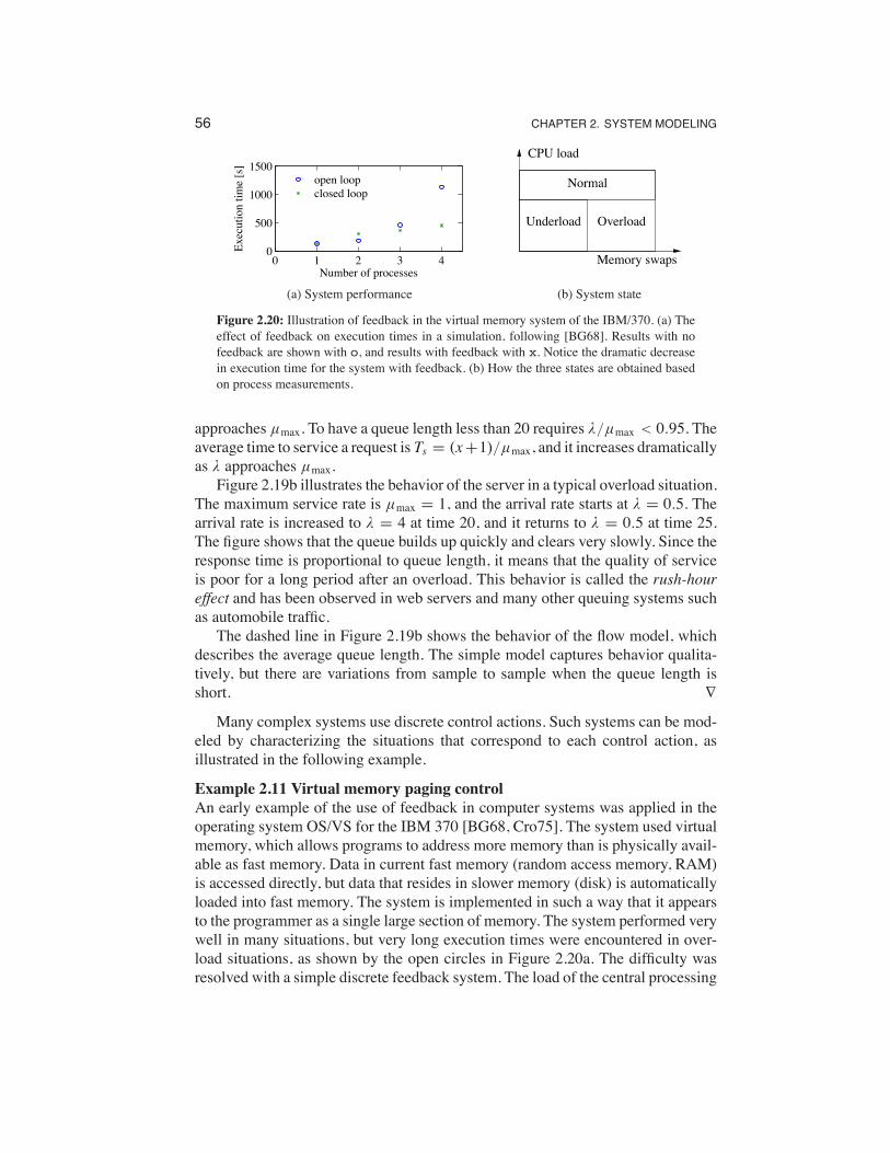
Figure 2.20: Illustration of feedback in the virtual memory system of the IBM/370. (a) Theeffect of feedback on execution times in a simulation, following [BG68]. Results with nofeedback are shown with o, and results with feedback with x. Notice the dramatic decreasein execution time for the system with feedback. (b) How the three states are obtained basedon process measurements.
approaches µmax. To have a queue length less than 20 requires ,/µmax < 0.95. Theaverage time to service a request is Ts = (x+1)/µmax, and it increases dramaticallyas , approaches µmax.Figure 2.19b illustrates the behavior of the server in a typical overload situation.
The maximum service rate is µmax = 1, and the arrival rate starts at , = 0.5. Thearrival rate is increased to , = 4 at time 20, and it returns to , = 0.5 at time 25.The figure shows that the queue builds up quickly and clears very slowly. Since theresponse time is proportional to queue length, it means that the quality of serviceis poor for a long period after an overload. This behavior is called the rush-houreffect and has been observed in web servers and many other queuing systems suchas automobile traffic.The dashed line in Figure 2.19b shows the behavior of the flow model, which
describes the average queue length. The simple model captures behavior qualita-tively, but there are variations from sample to sample when the queue length isshort. &
Many complex systems use discrete control actions. Such systems can be mod-eled by characterizing the situations that correspond to each control action, asillustrated in the following example.
Example 2.11 Virtual memory paging controlAn early example of the use of feedback in computer systems was applied in theoperating system OS/VS for the IBM 370 [BG68, Cro75]. The system used virtualmemory, which allows programs to address more memory than is physically avail-able as fast memory. Data in current fast memory (random access memory, RAM)is accessed directly, but data that resides in slower memory (disk) is automaticallyloaded into fast memory. The system is implemented in such a way that it appearsto the programmer as a single large section of memory. The system performed verywell in many situations, but very long execution times were encountered in over-load situations, as shown by the open circles in Figure 2.20a. The difficulty wasresolved with a simple discrete feedback system. The load of the central processing
2.4. MODELING EXAMPLES 57
4
5 2 31
(a) Sensor network
0 10 20 30 4010
20
30
40
Iteration
Age
nt st
ates
xi
(b) Consensus convergence
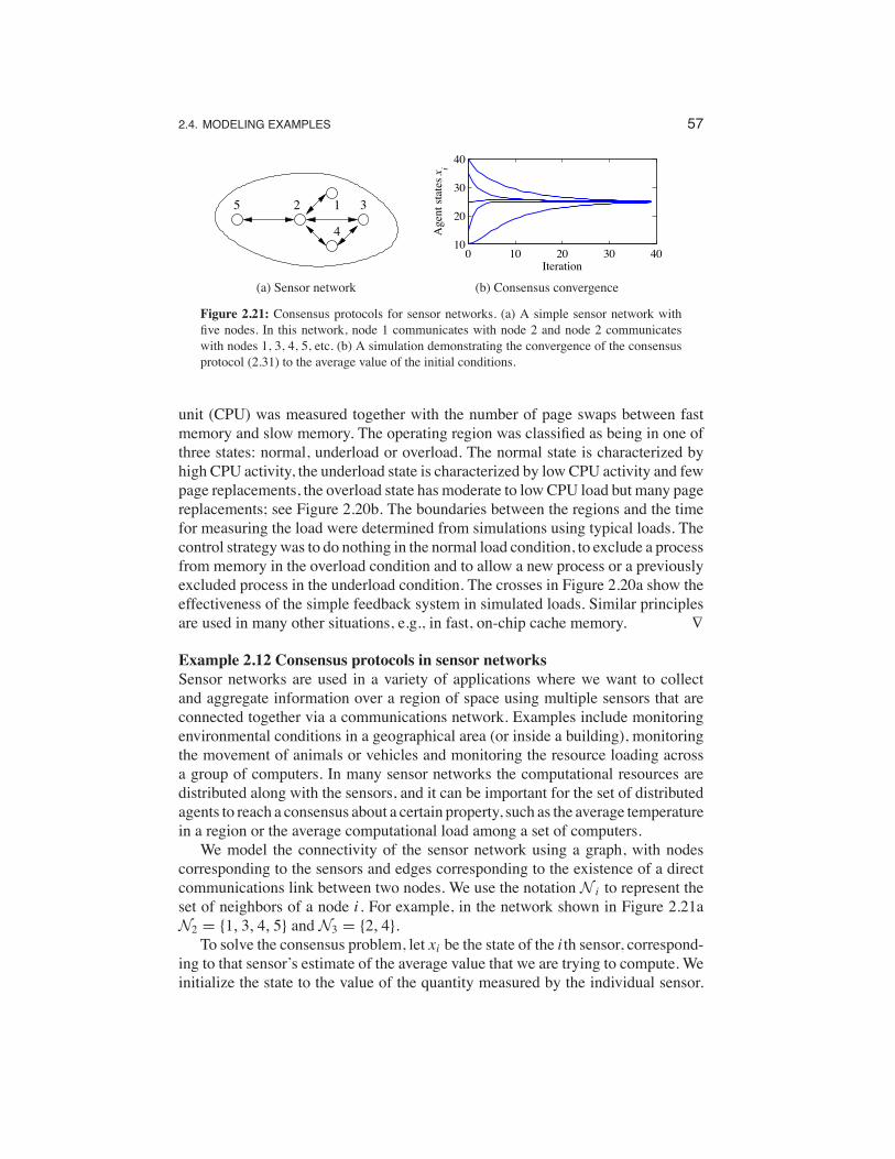
Figure 2.21: Consensus protocols for sensor networks. (a) A simple sensor network withfive nodes. In this network, node 1 communicates with node 2 and node 2 communicateswith nodes 1, 3, 4, 5, etc. (b) A simulation demonstrating the convergence of the consensusprotocol (2.31) to the average value of the initial conditions.
unit (CPU) was measured together with the number of page swaps between fastmemory and slow memory. The operating region was classified as being in one ofthree states: normal, underload or overload. The normal state is characterized byhigh CPU activity, the underload state is characterized by low CPU activity and fewpage replacements, the overload state has moderate to low CPU load but many pagereplacements; see Figure 2.20b. The boundaries between the regions and the timefor measuring the load were determined from simulations using typical loads. Thecontrol strategywas to do nothing in the normal load condition, to exclude a processfrom memory in the overload condition and to allow a new process or a previouslyexcluded process in the underload condition. The crosses in Figure 2.20a show theeffectiveness of the simple feedback system in simulated loads. Similar principlesare used in many other situations, e.g., in fast, on-chip cache memory. &
Example 2.12 Consensus protocols in sensor networksSensor networks are used in a variety of applications where we want to collectand aggregate information over a region of space using multiple sensors that areconnected together via a communications network. Examples include monitoringenvironmental conditions in a geographical area (or inside a building), monitoringthe movement of animals or vehicles and monitoring the resource loading acrossa group of computers. In many sensor networks the computational resources aredistributed along with the sensors, and it can be important for the set of distributedagents to reach a consensus about a certain property, such as the average temperaturein a region or the average computational load among a set of computers.We model the connectivity of the sensor network using a graph, with nodes
corresponding to the sensors and edges corresponding to the existence of a directcommunications link between two nodes. We use the notation N i to represent theset of neighbors of a node i . For example, in the network shown in Figure 2.21aN2 = {1, 3, 4, 5} and N3 = {2, 4}.To solve the consensus problem, let xi be the state of the i th sensor, correspond-
ing to that sensor’s estimate of the average value that we are trying to compute. Weinitialize the state to the value of the quantity measured by the individual sensor.
58 CHAPTER 2. SYSTEM MODELING
The consensus protocol (algorithm) can now be realized as a local update law
xi [k + 1] = xi [k]+ "&
j!Ni
(x j [k]" xi [k]). (2.31)
This protocol attempts to compute the average by updating the local state of eachagent based on the value of its neighbors. The combined dynamics of all agents canbe written in the form
x[k + 1] = x[k]" " (D " A)x[k], (2.32)
where A is the adjacency matrix and D is a diagonal matrix with entries corre-sponding to the number of neighbors of each node. The constant " describes therate at which the estimate of the average is updated based on information fromneighboring nodes. The matrix L := D " A is called the Laplacian of the graph.The equilibrium points of equation (2.32) are the set of states such that xe[k +
1] = xe[k]. It can be shown that xe = ((, (, . . . , () is an equilibrium state for thesystem, corresponding to each sensor having an identical estimate( for the average.Furthermore, we can show that ( is indeed the average value of the initial states.Since there can be cycles in the graph, it is possible that the state of the systemcould enter into an infinite loop and never converge to the desired consensus state.A formal analysis requires tools that will be introduced later in the text, but it canbe shown that for any connected graph we can always find a " such that the statesof the individual agents converge to the average. A simulation demonstrating thisproperty is shown in Figure 2.21b. &
Biological SystemsBiological systems provide perhaps the richest source of feedback and control ex-amples. The basic problem of homeostasis, in which a quantity such as temperatureor blood sugar level is regulated to a fixed value, is but one of themany types of com-plex feedback interactions that can occur in molecular machines, cells, organismsand ecosystems.
Example 2.13 Transcriptional regulationTranscription is the process by which messenger RNA (mRNA) is generated from asegment ofDNA.Thepromoter regionof a gene allows transcription to be controlledby the presence of other proteins, which bind to the promoter region and eitherrepress or activate RNA polymerase, the enzyme that produces an mRNA transcriptfrom DNA. The mRNA is then translated into a protein according to its nucleotidesequence. This process is illustrated in Figure 2.22.A simple model of the transcriptional regulation process is through the use
of a Hill function [dJ02, Mur04]. Consider the regulation of a protein A with aconcentration given by pa and a corresponding mRNA concentration ma . Let Bbe a second protein with concentration pb that represses the production of proteinA through transcriptional regulation. The resulting dynamics of pa and ma can be

2.4. MODELING EXAMPLES 59
RNApolymerase
DNA
Polypeptide
mRNA
RibosomeTranscription
Translation
Figure 2.22: Biological circuitry. The cell on the left is a bovine pulmonary cell, stained sothat the nucleus, actin and chromatin are visible. The figure on the right gives an overviewof the process by which proteins in the cell are made. RNA is transcribed from DNA by anRNA polymerase enzyme. The RNA is then translated into a protein by an organelle calleda ribosome.
written asdma
dt=
(ab1+ kab pnabb
+ (a0 " "ama,dpadt
= )ama " +a pa, (2.33)
where (ab+(a0 is the unregulated transcription rate, "a represents the rate of degra-dation of mRNA, (ab, kab and nab are parameters that describe how B represses A,)a represents the rate of production of the protein from its corresponding mRNAand +a represents the rate of degradation of the protein A. The parameter (a0 de-scribes the “leakiness” of the promoter, and nab is called the Hill coefficient andrelates to the cooperativity of the promoter.A similar model can be used when a protein activates the production of another
protein rather than repressing it. In this case, the equations have the formdma
dt=
(abkab pnabb1+ kab pnabb
+ (a0 " "ama,dpadt
= )ama " +a pa, (2.34)
where the variables are the same as described previously. Note that in the case ofthe activator, if pb is zero, then the production rate is (a0 (versus (ab + (a0 for therepressor). As pb gets large, the first term in the expression for ma approaches 1and the transcription rate becomes (ab + (a0 (versus (a0 for the repressor). Thuswe see that the activator and repressor act in opposite fashion from each other.As an example of how these models can be used, we consider the model of a
“repressilator,” originally due to Elowitz and Leibler [EL00]. The repressilator isa synthetic circuit in which three proteins each repress another in a cycle. This isshown schematically in Figure 2.23a, where the three proteins are TetR, ,cI andLacI. The basic idea of the repressilator is that if TetR is present, then it repressesthe production of ,cI. If ,cI is absent, then LacI is produced (at the unregulatedtranscription rate), which in turn represses TetR. Once TetR is repressed, then ,cI isno longer repressed, and so on. If the dynamics of the circuit are designed properly,the resulting protein concentrations will oscillate.We can model this system using three copies of equation (2.33), with A and
B replaced by the appropriate combination of TetR, cI and LacI. The state of the
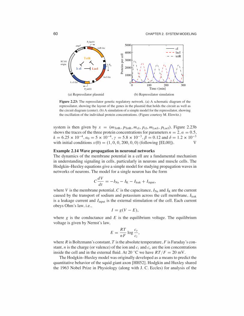
60 CHAPTER 2. SYSTEM MODELING
ampR
SC101 origin
PLtetO1
cI-lite
PR
lacI-lite
PLlacO1
tetR-lite
TetR
LacI cI
(a) Repressilator plasmid
0 100 200 3000
1000
2000
3000
4000
5000
Time t [min]
Prot
eins
per
cel
l
cI lacI tetR
(b) Repressilator simulation
Figure 2.23: The repressilator genetic regulatory network. (a) A schematic diagram of therepressilator, showing the layout of the genes in the plasmid that holds the circuit as well asthe circuit diagram (center). (b) A simulation of a simple model for the repressilator, showingthe oscillation of the individual protein concentrations. (Figure courtesy M. Elowitz.)
system is then given by x = (mTetR, pTetR,mcI, pcI,mLacI, pLacI). Figure 2.23bshows the traces of the three protein concentrations for parameters n = 2, ( = 0.5,k = 6.25# 10"4, (0 = 5# 10"4, " = 5.8# 10"3, ) = 0.12 and + = 1.2# 10"3
with initial conditions x(0) = (1, 0, 0, 200, 0, 0) (following [EL00]). &
Example 2.14 Wave propagation in neuronal networksThe dynamics of the membrane potential in a cell are a fundamental mechanismin understanding signaling in cells, particularly in neurons and muscle cells. TheHodgkin–Huxley equations give a simple model for studying propagation waves innetworks of neurons. The model for a single neuron has the form
CdVdt
= "INa " IK " Ileak + Iinput,
where V is the membrane potential,C is the capacitance, INa and IK are the currentcaused by the transport of sodium and potassium across the cell membrane, Ileakis a leakage current and Iinput is the external stimulation of the cell. Each currentobeys Ohm’s law, i.e.,
I = g(V " E),
where g is the conductance and E is the equilibrium voltage. The equilibriumvoltage is given by Nernst’s law,
E =RTnF
logceci
,
where R is Boltzmann’s constant, T is the absolute temperature, F is Faraday’s con-stant, n is the charge (or valence) of the ion and ci and ce are the ion concentrationsinside the cell and in the external fluid. At 20 ,C we have RT/F = 20 mV.The Hodgkin–Huxley model was originally developed as a means to predict the
quantitative behavior of the squid giant axon [HH52]. Hodgkin and Huxley sharedthe 1963 Nobel Prize in Physiology (along with J. C. Eccles) for analysis of the

2.5. FURTHER READING 61
electrical and chemical events in nerve cell discharges. The voltage clamp describedin Section 1.3 was a key element in Hodgkin and Huxley’s experiments. &
2.5 Further ReadingModeling is ubiquitous in engineering and science and has a long history in appliedmathematics. For example, the Fourier series was introduced by Fourier when hemodeled heat conduction in solids [Fou07]. Models of dynamics have been de-veloped in many different fields, including mechanics [Arn78, Gol53], heat con-duction [CJ59], fluids [BRS60], vehicles [Abk69, Bla91, Ell94], robotics [MLS94,SV89], circuits [Gui63], power systems [Kun93], acoustics [Ber54] and microme-chanical systems [Sen01]. Control theory requires modeling from many differ-ent domains, and most control theory texts contain several chapters on modelingusing ordinary differential equations and difference equations (see, for example,[FPEN05]). A classic book on the modeling of physical systems, especially me-chanical, electrical and thermofluid systems, is Cannon [Can03]. The book byAris [Ari94] is highly original and has a detailed discussion of the use of dimension-free variables. Two of the authors’ favorite books onmodeling of biological systemsare J. D. Murray [Mur04] and Wilson [Wil99].
Exercises2.1 (Chain of integrators form) Consider the linear ordinary differential equa-tion (2.7). Show that by choosing a state space representation with x1 = y, thedynamics can be written as
A =
!"""""""""""#
0 1 0
0 . . .. . . 0
0 · · · 0 1"an "an"1 "a1
$"""""""""""%
, B =
!"""""""""""#
00...1
$"""""""""""%
, C =!#1 . . . 0 0
$% .
This canonical form is called the chain of integrators form.
2.2 (Inverted pendulum) Use the equations of motion for a balance system to derivea dynamic model for the inverted pendulum described in Example 2.2 and verifythat for small ! the dynamics are approximated by equation (2.10).
2.3 (Disrete-time dynamics) Consider the following discrete-time system
x[k + 1] = Ax[k]+ Bu[k], y[k] = Cx[k],
where
x =!""#x1x2
$""% , A =
!""#a11 a120 a22
$""% , B =
!""#01
$""% , C =
!#1 0
$% .
62 CHAPTER 2. SYSTEM MODELING
In this problem, we will explore some of the properties of this discrete-time systemas a function of the parameters, the initial conditions and the inputs.
(a) For the case when a12 = 0 and u = 0, give a closed form expression for theoutput of the system.(b) A discrete system is in equilibrium when x[k + 1] = x[k] for all k. Let u = rbe a constant input and compute the resulting equilibrium point for the system.Show that if |aii | < 1 for all i , all initial conditions give solutions that converge tothe equilibrium point.(c) Write a computer program to plot the output of the system in response to a unitstep input, u[k] = 1, k + 0. Plot the response of your system with x[0] = 0 and Agiven by a11 = 0.5, a12 = 1 and a22 = 0.25.
2.4 (Keynesian economics) Keynes’ simple model for an economy is given by
Y [k] = C[k]+ I [k]+ G[k],
where Y , C , I and G are gross national product (GNP), consumption, investmentand government expenditure for year k. Consumption and investment are modeledby difference equations of the form
C[k + 1] = aY [k], I [k + 1] = b(C[k + 1]" C[k]),
where a and b are parameters. The first equation implies that consumption increaseswithGNPbut that the effect is delayed. The second equation implies that investmentis proportional to the rate of change of consumption.Show that the equilibrium value of the GNP is given by
Ye =1
1" a(Ie + Ge),
where the parameter 1/(1 " a) is the Keynes multiplier (the gain from I or G toY ). With a = 0.25 an increase of government expenditure will result in a fourfoldincrease of GNP. Also show that the model can be written as the following discrete-time state model:
!""#C[k + 1]I [k + 1]
$""% =
!""# a aab " b ab
$""%
!""#C[k]I [k]
$""% +
!""# aab
$""%G[k],
Y [k] = C[k]+ I [k]+ G[k].
2.5 (Least squares system identification) Consider a nonlinear differential equation!that can be written in the form
dxdt
=M&
i=1
(i fi (x),
where fi (x) are known nonlinear functions and (i are unknown, but constant,parameters. Suppose that we have measurements (or estimates) of the full state x

EXERCISES 63
at time instants t1, t2, . . . , tN , with N > M . Show that the parameters (i can bedetermined by finding the least squares solution to a linear equation of the form
H( = b,
where ( ! RM is the vector of all parameters and H ! RN#M and b ! RN areappropriately defined.2.6 (Normalized oscillator dynamics) Consider a damped spring–mass systemwithdynamics
mq + cq + kq = F.
Let #0 =(k/m be the natural frequency and - = c/(2
(km) be the damping
ratio.(a) Show that by rescaling the equations, we can write the dynamics in the form
q + 2-#0q + #20q = #20u, (2.35)
where u = F/k. This form of the dynamics is that of a linear oscillator with naturalfrequency #0 and damping ratio - .(b) Show that the system can be further normalized and written in the form
dz1d'
= z2,dz2d'
= "z1 " 2- z2 + v. (2.36)
The essential dynamics of the system are governed by a single damping parameter- . The Q-value defined as Q = 1/2- is sometimes used instead of - .2.7 (Electric generator) An electric generator connected to a strong power grid canbe modeled by a momentum balance for the rotor of the generator:
Jd2$dt2
= Pm " Pe = Pm "EVXsin $,
where J is the effective moment of inertia of the generator, $ the angle of rotation,Pm the mechanical power that drives the generator, Pe is the active electrical power,E the generator voltage,V the grid voltage and X the reactance of the line.Assumingthat the line dynamics are much faster than the rotor dynamics, Pe = V I =(EV/X) sin $, where I is the current component in phase with the voltage E and $is the phase angle between voltages E and V . Show that the dynamics of the electricgenerator has a normalized form that is similar to the dynamics of a pendulum withforcing at the pivot.2.8 (Admission control for a queue) Consider the queuing system described inExample 2.10. The long delays created by temporary overloads can be reduced byrejecting requests when the queue gets large. This allows requests that are acceptedto be serviced quickly and requests that cannot be accommodated to receive arejection quickly so that they can try another server. Consider an admission controlsystem described by
dxdt
= ,u " µmaxx
x + 1, u = sat(0,1)(k(r " x)), (2.37)
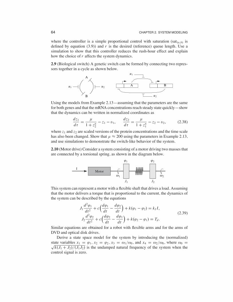
64 CHAPTER 2. SYSTEM MODELING
where the controller is a simple proportional control with saturation (sat(a,b) isdefined by equation (3.9)) and r is the desired (reference) queue length. Use asimulation to show that this controller reduces the rush-hour effect and explainhow the choice of r affects the system dynamics.
2.9 (Biological switch) A genetic switch can be formed by connecting two repres-sors together in a cycle as shown below.
u1
A
B
u2 B
u2
u1
A
Using the models from Example 2.13—assuming that the parameters are the samefor both genes and that the mRNA concentrations reach steady state quickly—showthat the dynamics can be written in normalized coordinates as
dz1d'
=µ
1+ zn2" z1 " v1,
dz2d'
=µ
1+ zn1" z2 " v2, (2.38)
where z1 and z2 are scaled versions of the protein concentrations and the time scalehas also been changed. Show that µ % 200 using the parameters in Example 2.13,and use simulations to demonstrate the switch-like behavior of the system.
2.10 (Motor drive) Consider a system consisting of a motor driving two masses thatare connected by a torsional spring, as shown in the diagram below.
MotorI
J1
1
1
J2
"
% 2%
2"
This system can represent a motor with a flexible shaft that drives a load. Assumingthat the motor delivers a torque that is proportional to the current, the dynamics ofthe system can be described by the equations
J1d2$1dt2
+ c,d$1dt
"d$2dt
.+ k($1 " $2) = kI I,
J2d2$2dt2
+ c,d$2dt
"d$1dt
.+ k($2 " $1) = Td .
(2.39)
Similar equations are obtained for a robot with flexible arms and for the arms ofDVD and optical disk drives.Derive a state space model for the system by introducing the (normalized)
state variables x1 = $1, x2 = $2, x3 = #1/#0, and x4 = #2/#0, where #0 =(k(J1 + J2)/(J1 J2) is the undamped natural frequency of the system when the
control signal is zero.