Chapter Twenty-nine ...................................................................................................................... 4 29-1.0 HYDROLOGIC DESIGN POLICIES................................................................................ 4

29-1.01 Introduction .................................................................................................................. 4 29-1.02 Surveys ......................................................................................................................... 4 29-1.03 Flood Hazards............................................................................................................... 4 29-1.04 Coordination ................................................................................................................. 4 29-1.05 Documentation.............................................................................................................. 5 29-1.06 Evaluation of Runoff Factors ....................................................................................... 5 29-1.07 Flood History................................................................................................................ 5

29-2.0 OVERVIEW....................................................................................................................... 6 29-2.01 Introduction .................................................................................................................. 6 29-2.02 Definition...................................................................................................................... 6 29-2.03 Factors Affecting Floods .............................................................................................. 6 29-2.04 Sources of Information ................................................................................................. 7

29-3.0 SYMBOLS AND DEFINITIONS...................................................................................... 7 29-4.0 CONCEPT DEFINITIONS ................................................................................................ 7 29-5.0 DESIGN FREQUENCY................................................................................................... 10

29-5.01 Overview .................................................................................................................... 10 29-5.02 Design Frequency ....................................................................................................... 10 29-5.03 Review Frequency ...................................................................................................... 11 29-5.04 Rainfall Curves ........................................................................................................... 11

29-6.0 HYDROLOGIC PROCEDURE SELECTION ................................................................ 12 29-6.01 Overview .................................................................................................................... 12 29-6.02 Peak Flow Rates or Hydrographs ............................................................................... 12 29-6.03 Hydrologic Methods ................................................................................................... 12

29-7.0 TIME OF CONCENTRATION ....................................................................................... 13 29-7.01 Overview .................................................................................................................... 13 29-7.02 Procedure .................................................................................................................... 14

29-7.02(01) Available Methods ........................................................................................... 14 29-7.02(02) Selection of Method......................................................................................... 14 29-7.02(03) Total Time of Concentration............................................................................ 14 29-7.02(04) Storm Drainage Systems.................................................................................. 15

29-7.03 NRCS Curve Number................................................................................................. 15 29-7.04 Kinematic Wave Equation.......................................................................................... 16 29-7.06 Federal Aviation ......................................................................................................... 18 29-7.07 NRCS Upland Method................................................................................................ 19 29-7.08 Triangular Gutter Flow............................................................................................... 20 29-7.09 Mannings� Equation ................................................................................................... 21

29-7.09(02) Open Channels ................................................................................................. 22 29-7.10 Continuity Equation.................................................................................................... 22 29-7.11 Reservoir or Lake ....................................................................................................... 22 29-7.12 Kerby .......................................................................................................................... 23 Example 29-7.7 ......................................................................................................................... 23

29-8.0 RATIONAL METHOD.................................................................................................... 26 29-8.01 Introduction ................................................................................................................ 26 29-8.02 Application ................................................................................................................. 26 29-8.03 Characteristics ............................................................................................................ 26 29-8.04 Equation...................................................................................................................... 27

29-8.05 Time of Concentration................................................................................................ 28 29-8.05(01) Storm Drainage Systems.................................................................................. 28 29-8.05(02) Common Errors................................................................................................ 29

29-8.06 Runoff Coefficient...................................................................................................... 29 29-8.07 Rainfall Intensity ........................................................................................................ 30 29-8.08 Example Problem (Rational Method)......................................................................... 30

29-9.0 USGS REGRESSION EQUATIONS .............................................................................. 32 29-9.01 Introduction ................................................................................................................ 32 29-9.02 Hydrologic Regions.................................................................................................... 32 29-9.03 Basin Characteristics .................................................................................................. 33 29-9.04 Regression Equations for Ungaged Sites.................................................................... 34 29-9.05 Procedure .................................................................................................................... 34

29-10.0 NRCS UNIT HYDROGRAPH ...................................................................................... 38 29-10.01 Introduction .............................................................................................................. 38 29-10.02 Application ............................................................................................................... 38 29-10.03 Equations and Concepts............................................................................................ 39 29-10.04 Procedure .................................................................................................................. 40

29-10.04(01) Runoff Factor ................................................................................................. 40 29-10.04(02) Time of Concentration ................................................................................... 41 29-10.04(03) Triangular Hydrograph Equation................................................................... 42

29-11.0 HEC 1 ............................................................................................................................. 43 29-12.0 REFERENCES ............................................................................................................... 44

List of Figures Figure Title 29-3A Hydrologic Symbols and Definitions 29-5A Design Frequency (Return Period - Years) 29-6A Selection of Discharge Computation Method 29-7A Methods for Calculating Time of Concentration 29-7B Roughness Coefficients (Manning�s n) for Sheet Flow 29-7C Values of N for Kerby�s Formula 29-8A Runoff Coefficients for the Rational Formula 29-8B Runoff Coefficients for the Rational Formula 29-8C Location of IDF Sites 29-8D Rainfall Intensity - Duration - Frequency Curve (Indianapolis, Indiana) 29-8E Rainfall Intensity - Duration - Frequency Curve (Louisville, Kentucky) 29-8F Rainfall Intensity - Duration - Frequency Curve (Bedford, Indiana)

29-8G Rainfall Intensity - Duration - Frequency Curve (Logansport, Indiana) 29-8H Rainfall Intensity - Duration - Frequency Curve (Richmond, Indiana) 29-8 I Rainfall Intensity - Duration - Frequency Curve (South Bend, Indiana) 29-8J Rainfall Intensity - Duration - Frequency Curve (Cincinnati, Ohio) 29-8K Rainfall Intensity - Duration - Frequency Curve (Evansville, Indiana) 29-8L Rainfall Intensity - Duration - Frequency Curve (Terre Haute, Indiana) 29-8M Rainfall Intensity - Duration - Frequency Curve (Chicago, Illinois) 29-8N Rainfall Intensity - Duration - Frequency Curve (Fort Wayne, Indiana) 29-9A Areas for Selecting Flood-Frequency USGS Estimating Equations 29-9B Mean Annual Precipitation (1941-1970) 29-9C Two-Year, 24-Hour Precipitation 29-9D Major Hydrologic Soil Groups 29-9E Prediction Equations, Standard Errors of the Estimate (SEE) and

Equivalent Years of Record (EY) 29-9F Ranges of Area Basin Characteristics for USGS Regression

Equations 29-10A Huff Distribution of Design Rainfall (50% Probability of Design

Rainfall) 29-10B NRCS Relation Between Direct Runoff, Curve Number and Precipitation 29-10C Runoff Curve Numbers � Urban Areas 29-10D Runoff Curve Numbers � Undeveloped Areas 29-10E Runoff Curve Numbers � Agricultural Lands 29-10F Conversion From Average Antecedent Moisture Conditions 29-10G Rainfall Groups for Antecedent Soil Moisture Conditions During

Growing and Dormant Seasons 29-10H Factors for Adjusting Lag (When Impervious Areas Occur in Watershed) 29-10 I Factors for Adjusting Lag (When Main Channel Has Been Hydraulically

Improved)

Chapter Twenty-nine

HYDROLOGY

29-1.0 HYDROLOGIC DESIGN POLICIES 29-1.01 Introduction Following is a summary of policies which apply to hydrologic analyses. For more information, refer to the AASHTO Highway Drainage Guidelines. 29-1.02 Surveys Hydrologic considerations can influence the selection of a highway corridor and the alternative routes within the corridor. Studies and investigations should be performed, including the consideration of the environmental and ecological impact of the project. The magnitude and complexity of these studies should be commensurate with the importance and magnitude of the project and the problems encountered. Typical data to be included in these surveys or studies are topographic maps, aerial photographs, streamflow records, historical highwater elevations, flood discharges and locations of hydraulic features such as reservoirs, water projects and designated or regulatory floodplain areas. 29-1.03 Flood Hazards A hydrologic analysis is a prerequisite to identifying flood hazard areas and determining those locations at which construction and maintenance will be unusually expensive or hazardous. 29-1.04 Coordination Interagency coordination is necessary because many levels of government plan, design and construct highway and water resource projects which might have an effect on each other. Agencies can share data and experiences within project areas to assist in the completion of accurate hydrologic analyses. The agencies include the Indiana Department of Natural Resources (IDNR), US Fish & Wildlife Service (USFS), US Army Corps of Engineers (USACOE),

Watershed Management Organizations, Natural Resources Conservation Service (NRCS), US Geological Survey (USGS), counties and cities. 29-1.05 Documentation The design of highway drainage facilities should be adequately documented. Frequently, it is necessary to refer to plans and specifications long after the actual construction has been completed. Documentation should include final computations, method of analysis selected, drainage area map, designer�s name and date, project correspondence relative to hydraulic considerations and permit information. See Section 28-5.0 for Department guidelines on documentation for hydrologic information. 29-1.06 Evaluation of Runoff Factors For all hydrologic analyses, the following factors must be evaluated and included if they will have a significant effect on the final results: 1. Drainage basin characteristics including size, shape, slope, land use, geology, soil type,

surface infiltration and storage. 2. Stream channel characteristics including geometry and configuration, natural and

artificial controls, channel modification, aggradation/degradation, and ice and debris. 3. Flood plain characteristics. 4. Meteorological characteristics such as precipitation amounts and type, distribution

characteristics and time rate of precipitation (hyetograph). 5. Where appropriate, the designer should evaluate future land use changes that might occur

during the service life of the proposed facility and that could result in inadequate drainage systems.

29-1.07 Flood History All hydrologic analyses must consider the flood history of the area and the effect of these historical floods on existing and proposed structures. The flood history must include the historical floods and the flood history of any existing structures.

29-2.0 OVERVIEW 29-2.01 Introduction The analysis of the peak rate of runoff, volume of runoff and time distribution of flow is fundamental to the design of drainage facilities. The design of each highway drainage facility requires the determination of discharge-frequency relationships. The design of some facilities require a peak flow rate while others require a runoff hydrograph providing an estimate of runoff volume. The peak flow rates are most often used in the design of bridges, culverts, roadside ditches and small storm sewer systems. Drainage systems involving detention storage, pumping stations and large or complex storm sewer systems require the development of a runoff hydrograph. Errors in the estimates will result in a structure that is either undersized, and causes more drainage problems, or oversized, and costs more than necessary. However, it must be realized that any hydrologic analysis is only an approximation. The relationship between the amount of precipitation on a drainage basin and the amount of runoff from the basin is complex, and insufficient data is available concerning the factors influencing the rural and urban rainfall-runoff relationship to expect exact solutions. 29-2.02 Definition Hydrology is generally defined as a science which explores the interrelationship between water on and under the earth and in the atmosphere. For the Indiana Design Manual, hydrology will address estimating flood magnitudes as the result of precipitation. In the design of highway drainage structures, floods are usually considered in terms of peak runoff or discharge in cubic meters per second (m3/s) and hydrographs as discharge per time. For structures which are designed to control the volume of runoff (e.g., detention storage facilities) or where flood routing through culverts is used, then the entire discharge hydrograph will be of interest. Wetland hydrology, the water-related driving force to create wetlands, is addressed in the AASHTO Highway Drainage Guidelines, Volume X. 29-2.03 Factors Affecting Floods In the hydrologic analysis for a drainage structure, the designer must recognize that there are many variables that affect floods. Some of the factors which must be considered on an individ-ual site-by-site basis include the following: 1. rainfall amount and storm distribution;

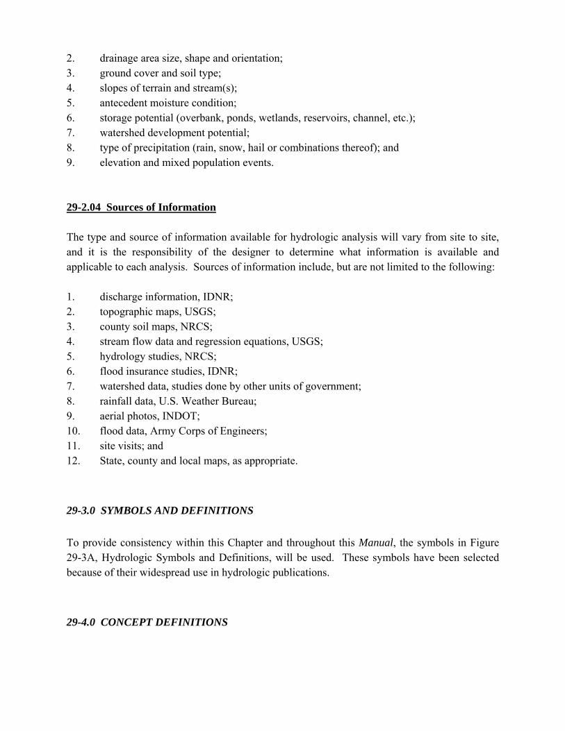
2. drainage area size, shape and orientation; 3. ground cover and soil type; 4. slopes of terrain and stream(s); 5. antecedent moisture condition; 6. storage potential (overbank, ponds, wetlands, reservoirs, channel, etc.); 7. watershed development potential; 8. type of precipitation (rain, snow, hail or combinations thereof); and 9. elevation and mixed population events. 29-2.04 Sources of Information The type and source of information available for hydrologic analysis will vary from site to site, and it is the responsibility of the designer to determine what information is available and applicable to each analysis. Sources of information include, but are not limited to the following: 1. discharge information, IDNR; 2. topographic maps, USGS; 3. county soil maps, NRCS; 4. stream flow data and regression equations, USGS; 5. hydrology studies, NRCS; 6. flood insurance studies, IDNR; 7. watershed data, studies done by other units of government; 8. rainfall data, U.S. Weather Bureau; 9. aerial photos, INDOT; 10. flood data, Army Corps of Engineers; 11. site visits; and 12. State, county and local maps, as appropriate.

29-3.0 SYMBOLS AND DEFINITIONS To provide consistency within this Chapter and throughout this Manual, the symbols in Figure 29-3A, Hydrologic Symbols and Definitions, will be used. These symbols have been selected because of their widespread use in hydrologic publications.

29-4.0 CONCEPT DEFINITIONS

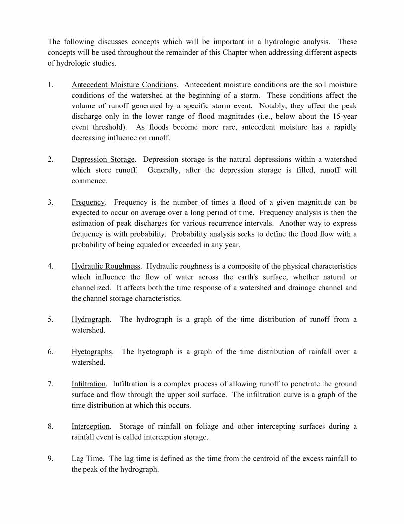
The following discusses concepts which will be important in a hydrologic analysis. These concepts will be used throughout the remainder of this Chapter when addressing different aspects of hydrologic studies. 1. Antecedent Moisture Conditions. Antecedent moisture conditions are the soil moisture

conditions of the watershed at the beginning of a storm. These conditions affect the volume of runoff generated by a specific storm event. Notably, they affect the peak discharge only in the lower range of flood magnitudes (i.e., below about the 15-year event threshold). As floods become more rare, antecedent moisture has a rapidly decreasing influence on runoff.

2. Depression Storage. Depression storage is the natural depressions within a watershed

which store runoff. Generally, after the depression storage is filled, runoff will commence.

3. Frequency. Frequency is the number of times a flood of a given magnitude can be

expected to occur on average over a long period of time. Frequency analysis is then the estimation of peak discharges for various recurrence intervals. Another way to express frequency is with probability. Probability analysis seeks to define the flood flow with a probability of being equaled or exceeded in any year.

4. Hydraulic Roughness. Hydraulic roughness is a composite of the physical characteristics

which influence the flow of water across the earth's surface, whether natural or channelized. It affects both the time response of a watershed and drainage channel and the channel storage characteristics.

5. Hydrograph. The hydrograph is a graph of the time distribution of runoff from a

watershed. 6. Hyetographs. The hyetograph is a graph of the time distribution of rainfall over a

watershed. 7. Infiltration. Infiltration is a complex process of allowing runoff to penetrate the ground

surface and flow through the upper soil surface. The infiltration curve is a graph of the time distribution at which this occurs.

8. Interception. Storage of rainfall on foliage and other intercepting surfaces during a

rainfall event is called interception storage. 9. Lag Time. The lag time is defined as the time from the centroid of the excess rainfall to

the peak of the hydrograph.

10. Peak Discharge. The peak discharge, sometimes called peak flow, is the maximum rate

of flow of water passing a given point during or after a rainfall event or snow melt. 11. Rainfall Excess. The rainfall excess is the water available to runoff after interception,

depression storage and infiltration have been satisfied. 12. Rainfall Intensity. The amount of rainfall occurring in a unit of time, converted to its

equivalent in mm per hour. 13. Recurrence Interval. The average number of years between occurrences of a discharge or

rainfall that equals or exceeds the given magnitude. 14. Runoff. The portion of the precipitation which runs off the surface of a drainage area

after all abstractions are accounted for. 15. Runoff Coefficient. A factor representing the portion of runoff resulting from a unit

rainfall. It is dependent on topography, land use and soil characteristics. 16. Stage. The stage of a river is the elevation of the water surface above some elevation

datum. 17. Time Of Concentration. The time of concentration is the time it takes the drop of water

falling on the hydraulically most remote point in the watershed to travel through the watershed to the point under investigation.

18. Ungaged Stream Sites. Locations at which no systematic records are available for actual

stream flows. 19. Unit Hydrograph. A unit hydrograph is the direct runoff hydrograph resulting from a

rainfall event which has a specific temporal and spatial distribution, which lasts for a specific duration, and which has unit volume (or results from a unit depth of rainfall). The ordinates of the unit hydrograph are such that the volume of direct runoff represented by the area under the hydrograph is equal to one millimeter of runoff from the drainage area. When a unit hydrograph is shown with units of cubic meters per second, it is implied that the ordinates are cubic meters per second per millimeter of direct runoff.

For a more complete discussion of these concepts and others related to hydrologic analysis, the reader is referred to Hydrologic Design For Highways, Federal Highway Administration, Hydraulic Design Series 2, 1995, and Guidelines for Hydrology - Volume II Highway Drainage Guidelines, prepared by the Task Force On Hydrology and Hydraulics, AASHTO Highway Subcommittee on Design.

29-5.0 DESIGN FREQUENCY 29-5.01 Overview Because it is not economically feasible to design a structure for the maximum runoff a watershed is capable of producing, a design frequency must be established. The design frequency for a given flood is defined as the reciprocal of the probability or chance that a flood will be equaled or exceeded in a given year. If a flood has a 20 percent chance of being equaled or exceeded each year over a long period of time, the flood will be equaled or exceeded on average once every five years. This is called the return period or recurrence interval (RI). Thus, the exceedence probability equals 100/RI. The designer should note that the 5-year flood is not one that will necessarily be equaled or exceeded every five years. There is a 20 percent chance that the flood will be equaled or exceeded in any year; therefore, the 5-year flood could conceivably occur in several consecutive years. The same reasoning applies to floods with other return periods. INDOT has related design frequency to roadway serviceability. Roadway serviceability may be defined as travel lanes open to traffic with no flood waters encroaching into the travel lanes during a design storm. The higher functional classes of highway require design flood frequencies of less frequent storms than lower functional classes of highway. 29-5.02 Design Frequency The design frequency used to design a hydraulic facility is determined by the type, size and location of the structure. The following applies to the design frequency for the indicated drainage application: 1. Cross Drainage. A drainage facility shall be designed to accommodate a discharge with a

given return period(s) for the following circumstances. The design shall be such that the backwater (the headwater) caused by the structure for the design storm does not:

a. increase the flood hazard significantly for property, b. overtop the highway, or c. exceed a certain depth on the highway embankment.

Based on these design criteria, a design involving temporary roadway overtopping for floods larger than the design event is acceptable practice. Usually, if overtopping is

allowed, the structure may be designed to accommodate a flood of a lesser frequency without overtopping.

2. Storm Drains. A storm drain shall be designed to accommodate a discharge with a given

return period(s) for the following circumstances. The design shall be such that the storm runoff does not:

a. increase the flood hazard significantly for property; b. encroach onto the street or highway so as to cause a significant traffic hazard; or c. limit traffic, emergency vehicles, or pedestrian movement to an unreasonable

extent.

Based on these design criteria, a design involving temporary street or road inundation for floods larger than the design event is acceptable practice.

See Figure 29-5A, Design Frequency (Return Period � Years). 29-5.03 Review Frequency Where appropriate, the design of hydraulic structures should include an assessment of flood hazards inherent in the proposed facility for frequencies other than the design frequency. After sizing a drainage facility using a flood and sometimes the hydrograph corresponding to the design frequency, it is necessary to review the proposed facility with a base discharge. This is done to ensure that there are no unexpected flood hazards inherent in the proposed facility(ies). Where the design Q is less than Q100, the review flood shall be the 100-year event. When available, discharges should be obtained from the coordinated discharge curves, which are in the IDNR publication Coordinated Discharges of Selected Streams in Indiana and in FEMA/NFIP publications. Potential impacts to consider include possible flood damage due to high embankments where overtopping is not practical, back up due to the presence of median barriers or noise walls, and flood damage due to a storm sewer back up. Potential scour damage to a bridge substructure should be reviewed for the 500-year frequency. 29-5.04 Rainfall Curves Rainfall data are available for many geographic areas. From these data, rainfall intensity-duration-frequency (IDF) curves have been developed for the commonly used design frequencies. The IDF curves for locations in Indiana are in Section 29-8. These curves have

been developed using HYDRAIN�s HYDRO module, and they are based on the National Weather Service (NWS) technical memorandum, HYDRO-35 (Frederick, et. al., 1976). HYDRO may be used to develop the IDF for any specific location with known latitude and longitude for durations up to 60 minutes.

29-6.0 HYDROLOGIC PROCEDURE SELECTION 29-6.01 Overview Streamflow measurements for determining a flood frequency relationship at a site are usually unavailable; in such cases, it is accepted practice to estimate peak runoff rates and hydrographs using statistical or empirical methods. In general, results from using several methods should be compared, not averaged. The designer should review the design discharge for other structures on the stream and historical data and consider previous studies including flood insurance studies. INDOT�s practice is to use the discharge that best reflects local project conditions with the reasons documented. The following discusses INDOT�s use for each procedure. 29-6.02 Peak Flow Rates or Hydrographs A consideration of peak runoff rates for the design conditions is generally adequate for conveyance systems such as storm drains or open channels. However, if the design must include flood routing (e.g., storage basins, complex conveyance networks), a flood hydrograph is usually required. Although the development of runoff hydrographs (typically more complex than estimating peak runoff rates) is often accomplished using computer programs, some methods are adaptable to nomographs or other desktop procedures. 29-6.03 Hydrologic Methods Where feasible, for large structures, several methods of computing discharge should be checked, comparing the results to what other structures in the area are designed for and the historical data for the area. Engineering judgment should then be used to select the discharge. If practical, the method should be calibrated to local conditions and tested for accuracy and reliability. Figure 29-6A, Selection of Discharge Computation Method, summarizes the recommended hydrologic methods currently acceptable for use in the design of highway structures in Indiana and their application. The following provides additional guidance on the selection of hydrologic methods.

1. IDNR Coordinated Discharge Curves. This is the preferred method on rural and urban

streams for which the information is available. The reference is Coordinated Discharges of Selected Streams in Indiana.

2. IDNR Letter of Discharge. The IDNR Letter of Discharge must be prepared for

structures that require a Construction in a Floodway Permit. 3. NRCS (formerly SCS) Unit Hydrograph Method (TR-20). This method can be used to

determine peak discharges and hydrographs in rural areas for any basin size. 4. HEC I. This hydrograph method can be used to determine peak discharges and

hydrographs in rural areas for any basin size and in urban areas with large watersheds. 5. Indiana USGS Regression Equations. This method can be used in rural areas for

estimating when no other methods are available. 6. Rational Method. This is the preferred method for developed areas. It can be used for

drainage areas less than 40 ha in urban areas and less than 80 ha in rural areas. 7. FEMA. The 100-year discharges specified in the applicable FEMA flood insurance study

shall be used to analyze impacts of a proposed crossing on a regulatory floodway. However, if these discharges are considered outdated, the discharges based on current methods may be used subject to receiving the necessary regulatory approvals.

8. Frequency Analysis of Stream Gaging Records. The IDNR Division of Water maintains

a database of discharges for various frequencies computed using methodologies contained in Bulletin 17B of the Water Resources Council. Comparisons of discharges computed for nearby gages can be of great value.

29-7.0 TIME OF CONCENTRATION 29-7.01 Overview The time of concentration (tC) is the time required for water to flow from the hydraulically most remote point of the drainage area to the point under investigation. Time of concentration is an important variable in many hydrologic methods, including the Rational and Natural Resources Conservation Service (formerly SCS) procedures. For the same size watershed, the shorter the tC, the larger the peak discharge.

29-7.02 Procedure Water moves through a watershed as a combination of overland and channelized flow. The type that occurs is a function of the conveyance system and is best determined by field inspection. When designing a drainage system, the overland flow path is not necessarily perpendicular to the contours shown on available mapping. Often the land will be graded and swales will intercept the natural contour and conduct the water to the streets which reduces the time of concentration. Generally, the overland flow path should be less than 60 m in urban areas and 90 m in rural areas.

29-7.02(01) Available Methods See Figure 29-7A, Methods for Calculating Time of Concentration.

29-7.02(02) Selection of Method The methods included in this Chapter are generally applicable for both the Rational Equation and the NRCS (formerly SCS) Peak Flow or Hydrograph Methods. The Rational Equation normally uses tC in minutes; NRCS procedures generally use tC in hours. To choose a method, consider the conditions for which the equation was developed and how they compare to the drainage area being designed. When NRCS methods will be used to compute discharge, time of concentration should be determined using the methods recommended by the NRCS.

29-7.02(03) Total Time of Concentration To obtain the total time of concentration, the channel flow time must be calculated and added to the overland flow time. After first determining the average flow velocity in the pipe or channel, the travel time is obtained by dividing velocity into the pipe or channel length.

(V)(60)L = t t (Equation 29-7.1)

Where: tt = travel time, minutes

L = length which runoff must travel, m V = estimated or calculated velocity, m/s

The total time of concentration is:

t t + t = t oc (Equation 29-7.2)

Where: tC = total time of concentration

tO = overland flow time tt = travel time

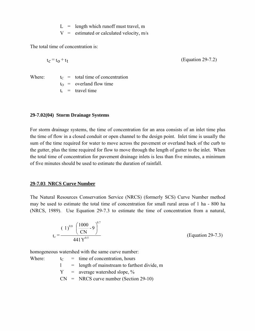
29-7.02(04) Storm Drainage Systems For storm drainage systems, the time of concentration for an area consists of an inlet time plus the time of flow in a closed conduit or open channel to the design point. Inlet time is usually the sum of the time required for water to move across the pavement or overland back of the curb to the gutter, plus the time required for flow to move through the length of gutter to the inlet. When the total time of concentration for pavement drainage inlets is less than five minutes, a minimum of five minutes should be used to estimate the duration of rainfall. 29-7.03 NRCS Curve Number The Natural Resources Conservation Service (NRCS) (formerly SCS) Curve Number method may be used to estimate the total time of concentration for small rural areas of 1 ha - 800 ha (NRCS, 1989). Use Equation 29-7.3 to estimate the time of concentration from a natural,

homogeneous watershed with the same curve number:

Y441

9 - CN

1000 )1 ( = t 0.5

0.70.8

c (Equation 29-7.3)

Where: tC = time of concentration, hours l = length of mainstream to farthest divide, m Y = average watershed slope, % CN = NRCS curve number (Section 29-10)

The above equation should only be used for rural watersheds with a flow length between 60 m and 7900 m and a Y (average watershed slope) between 0.5% and 64%. This method is included in HYDRO as an option for calculating tC.

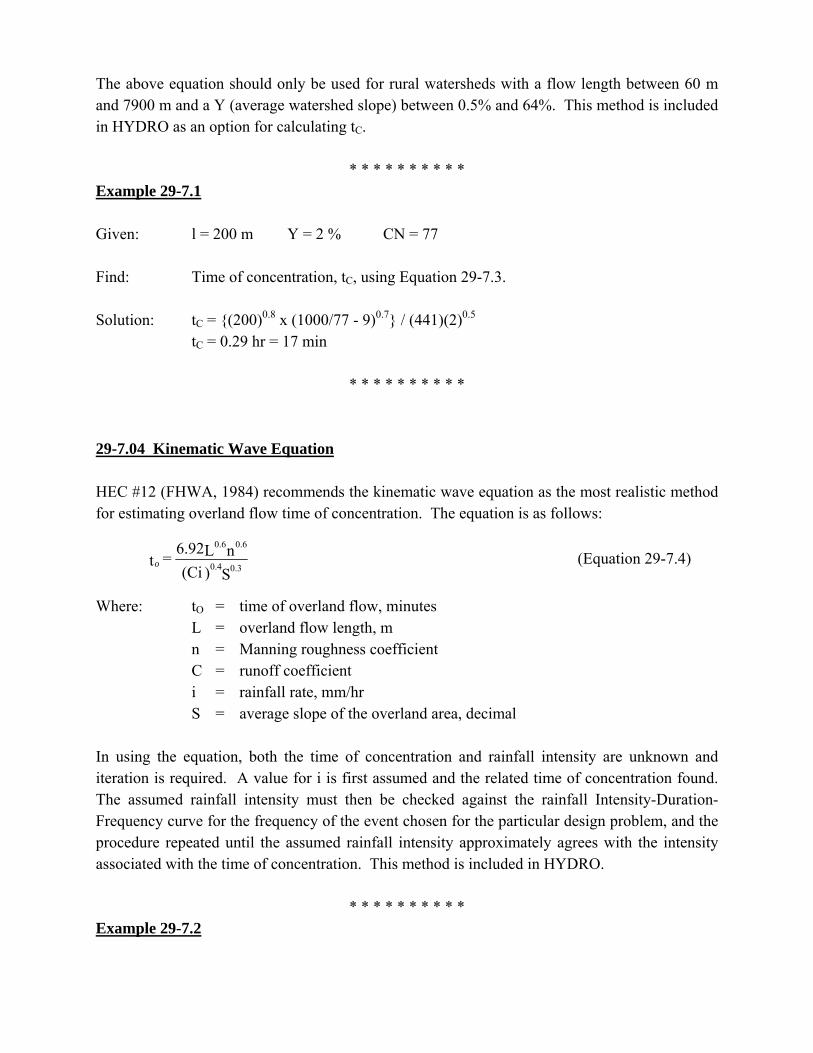
* * * * * * * * * * Example 29-7.1 Given: l = 200 m Y = 2 % CN = 77 Find: Time of concentration, tC, using Equation 29-7.3. Solution: tC = {(200)0.8 x (1000/77 - 9)0.7} / (441)(2)0.5

tC = 0.29 hr = 17 min

* * * * * * * * * * 29-7.04 Kinematic Wave Equation HEC #12 (FHWA, 1984) recommends the kinematic wave equation as the most realistic method for estimating overland flow time of concentration. The equation is as follows:

S)(CinL6.92 = t 0.30.4

0.60.6

o (Equation 29-7.4)

Where: tO = time of overland flow, minutes L = overland flow length, m n = Manning roughness coefficient C = runoff coefficient i = rainfall rate, mm/hr S = average slope of the overland area, decimal

In using the equation, both the time of concentration and rainfall intensity are unknown and iteration is required. A value for i is first assumed and the related time of concentration found. The assumed rainfall intensity must then be checked against the rainfall Intensity-Duration-Frequency curve for the frequency of the event chosen for the particular design problem, and the procedure repeated until the assumed rainfall intensity approximately agrees with the intensity associated with the time of concentration. This method is included in HYDRO.

* * * * * * * * * * Example 29-7.2

Given: L = 45 m S = 0.02

n = 0.24 (dense grass) C = 0.40 (impervious soils with turf) Design frequency = 10 yr Location: Indianapolis, IN

Find: Overland flow time, tO, using Equation 29-7.4. Solution: 1. Assume i = 120 mm/hr and calculate tO:

)(0.02 )120 x (0.40)(0.24 )6.92(45 = t 0.30.4

0.60.6

o

minutes 20 = to

2. Based on calculated tO, find i from Figure 29-8D, Rainfall Intensity-Duration-Frequency

Curve (Indianapolis, Indiana):

i = 100 mm/hr 3. Assume i = 100 mm/hr and calculate tO:

)(0.02 )100 x (0.40)(0.24 )6.92(45 = t 0.30.4

0.60.6

o

minutes 21 = to 4. Based on calculated tO, find i from Figure 29-8D.

i = 98 mm/hr assumed 100 mm/hr; therefore, tO = 21 min 29-7.05 Manning’s Kinematic Solution For sheet (overland) flow of less than 90 m, TR-55 (NRCS, 1986) recommends Manning�s kinematic solution (Overton and Meadows, 1976) to compute to. This method is included in the TR-55 computer program. The equation is:

S)P()(nL0.091 = t 0.40.5

2

0.8

o (Equation 29-7.5)

Where: tO = overland flow time, hr n = Manning�s roughness coefficient, Figure 29-7B, Roughness Coefficients

for the Rational Formula L = flow length, m P2 = 2-year, 24-hour rainfall, mm (from TP-40) S = slope of hydraulic grade line (land slope), decimal

This simplified form of the Manning�s kinematic solution is based on: 1. shallow steady uniform flow, 2. constant intensity of rainfall excess (rain available for runoff), 3. rainfall duration of 24 hours, and 4. minor effect of infiltration on travel time Note that this overland time of concentration is acceptable for use within the TR-20 hydrologic methodology.

* * * * * * * * * Example 29-7.3 Given: L = 45 m S = 0.02 n = 0.24 (Dense Grass)

Location: Indianapolis, IN Find: Overland flow time, tO, using Equation 29-7.5. Solution: 1. For Indianapolis, P2 = 65 mm from TP 40

)(0.02)(65)4)(45)0.091((0.2 = t 0.40.5

0.8

o 2.

tO = 0.36 hr = 21.7 min

* * * * * * * * * * 29-7.06 Federal Aviation For design conditions that do not involve complex drainage conditions, the Federal Aviation Equation (FAA, 1970) can be used to estimate overland flow time. Equation 29-7.6 was

S 1.44LC) - (1.1 = t 0.33

0.5

o (Equation 29-7.6)

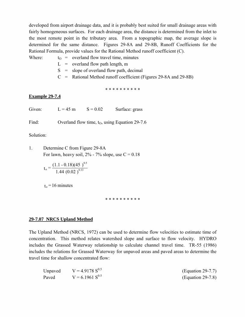
developed from airport drainage data, and it is probably best suited for small drainage areas with fairly homogeneous surfaces. For each drainage area, the distance is determined from the inlet to the most remote point in the tributary area. From a topographic map, the average slope is determined for the same distance. Figures 29-8A and 29-8B, Runoff Coefficients for the Rational Formula, provide values for the Rational Method runoff coefficient (C). Where: tO = overland flow travel time, minutes

L = overland flow path length, m S = slope of overland flow path, decimal C = Rational Method runoff coefficient (Figures 29-8A and 29-8B)

* * * * * * * * * *

Example 29-7.4 Given: L = 45 m S = 0.02 Surface: grass Find: Overland flow time, tO, using Equation 29-7.6 Solution: 1. Determine C from Figure 29-8A

For lawn, heavy soil, 2% - 7% slope, use C = 0.18

)(0.02 1.44)0.18)(45 - (1.1 = t 0.33

0.5

o

minutes 16 = ot

* * * * * * * * * * 29-7.07 NRCS Upland Method The Upland Method (NRCS, 1972) can be used to determine flow velocities to estimate time of concentration. This method relates watershed slope and surface to flow velocity. HYDRO includes the Grassed Waterway relationship to calculate channel travel time. TR-55 (1986) includes the relations for Grassed Waterway for unpaved areas and paved areas to determine the travel time for shallow concentrated flow:

Unpaved V = 4.9178 S0.5 (Equation 29-7.7) Paved V = 6.1961 S0.5 (Equation 29-7.8)

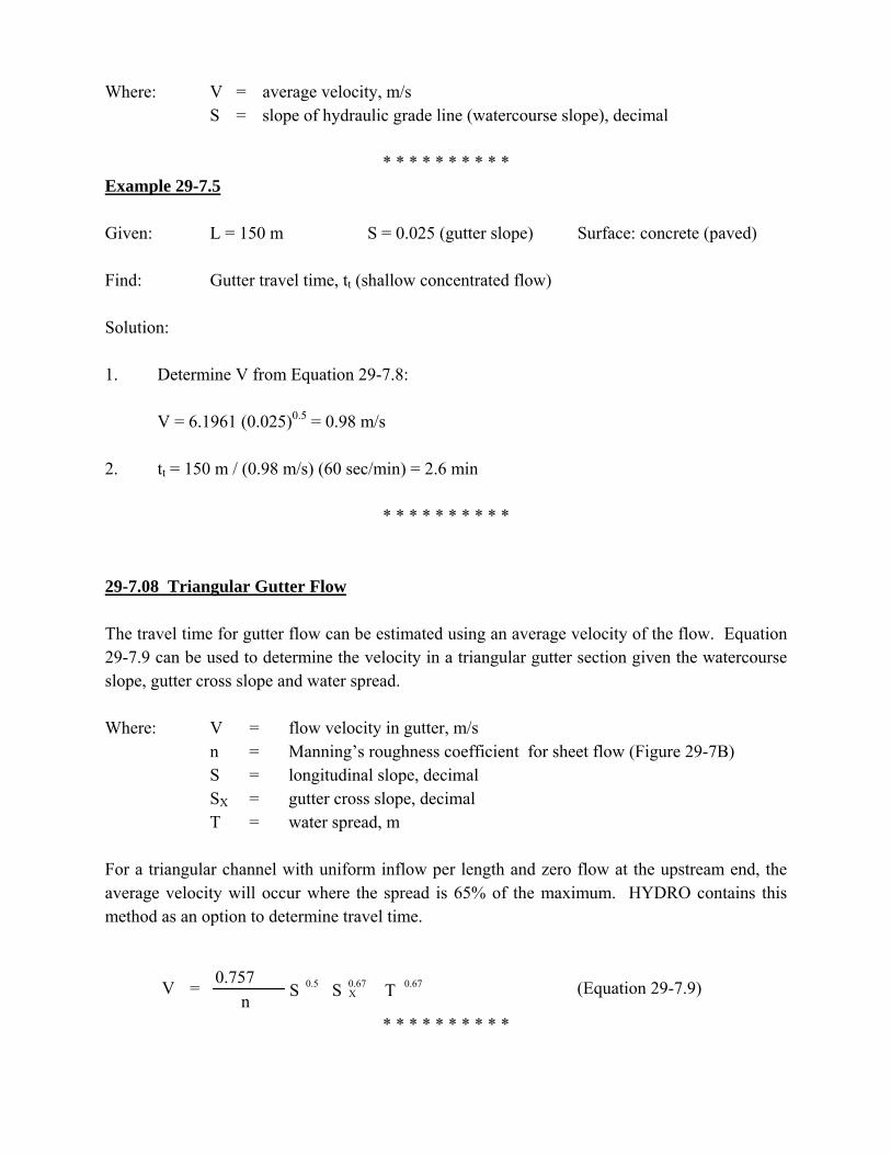
Where: V = average velocity, m/s S = slope of hydraulic grade line (watercourse slope), decimal

* * * * * * * * * *

Example 29-7.5 Given: L = 150 m S = 0.025 (gutter slope) Surface: concrete (paved) Find: Gutter travel time, tt (shallow concentrated flow) Solution: 1. Determine V from Equation 29-7.8:

V = 6.1961 (0.025)0.5 = 0.98 m/s 2. tt = 150 m / (0.98 m/s) (60 sec/min) = 2.6 min

* * * * * * * * * * 29-7.08 Triangular Gutter Flow The travel time for gutter flow can be estimated using an average velocity of the flow. Equation 29-7.9 can be used to determine the velocity in a triangular gutter section given the watercourse slope, gutter cross slope and water spread. Where: V = flow velocity in gutter, m/s

n = Manning�s roughness coefficient for sheet flow (Figure 29-7B) S = longitudinal slope, decimal SX = gutter cross slope, decimal T = water spread, m

For a triangular channel with uniform inflow per length and zero flow at the upstream end, the average velocity will occur where the spread is 65% of the maximum. HYDRO contains this method as an option to determine travel time.

* * * * * * * * * *

T S S n0.757 = V 0.670.67

X0.5 (Equation 29-7.9)

Example 29-7.6 Given: S = 0.025 (longitudinal slope) SX = 0.02 (cross slope)

T = 3 m (design spread at inlet) L = 150 m (flow length) n = 0.016 (concrete)

Find: Travel time of flow in gutter Solution: 1. Use Tavg = 0.65 Tdesign = 0.65 x 3 = 1.95 m 2. From Equation 29-7.9:

)(1.95 )(0.02 )(0.025 0.0160.757 = V 0.670.670.5

m/s0.85 = V

3. From Equation 29-7.1:

tt = 150 m / (0.85 m/s) (60 sec/min) = 2.9 min

* * * * * * * * * * 29-7.09 Mannings’ Equation In watersheds with storm drains or channels, the travel time must be added to the overland flow time to find the total time of concentration where appropriate. The velocity can be determined

using Manning�s equation:

SRn1.0 = V 2/13/2 (Equation 29-7.10)

Where: V = mean velocity of flow, m/s n = Manning�s roughness coefficient R = hydraulic radius (m) = Area/Wetted Perimeter S = slope of the hydraulic grade line, decimal

29-7.09(01) Pipe Flow

For ordinary conditions, storm drains should be sized assuming that they will flow full or almost full for the design discharge. For non-pressure flow, the velocity can be determined using Manning�s equation. For circular pipes flowing full, the equation becomes:

SDn0.397 = V 2/13/2 (Equation 29-7.11)

Where: D = diameter of circular pipe, m Pipe flow charts can be used to determine the velocity for either full or partially full flow conditions.

29-7.09(02) Open Channels Open channels are assumed to begin where the surveyed cross section information has been obtained, where channels are visible on aerial photographs, or where blue lines (indicating streams) appear on United States Geological Survey (USGS) quadrangle sheets. Manning�s equation or the water surface profile information can be used to estimate average flow velocity. Equation 29-7.10 can be used to solve Manning�s equation. Average flow velocity is usually determined for bank-full elevation. 29-7.10 Continuity Equation If the pipes of a storm drainage system will operate under pressure flow, the continuity equation should be used to determine velocity.

V = Q/A (Equation 29-7.12) Where: V = mean velocity of flow, m/s

Q = discharge in pipe, m3/s A = area of pipe, m2

29-7.11 Reservoir or Lake Occasionally, it is necessary to compute tc for a watershed having a relatively large body of water within its flow path. In these cases, tc is computed to the upstream end of the lake or

reservoir and, for the body of water, the travel time is computed using the following equation (King, 1967).

Vw = (gDm)0.5 (Equation 29-7.13) Where: Vw = the wave velocity across the water, m/s

g = 9.81 m/sec2 Dm = mean depth of lake or reservoir, m

Generally, Vw will be high (2.5 m/s to 9 m/s). Equation 29-7.13 only estimates travel time across the lake. It does not account for the travel time involved with the passage of the inflow hydrograph through spillway storage and the reservoir or lake outlet. This time is generally much longer and is added to the travel time across the lake. The travel time through lake storage and its outlet can be determined by the storage routing procedures in Chapter Thirty-five. Equation 29-7.13 can be used for swamps with considerable open water but, where the vegetation or debris is relatively thick (less than about 25 percent open water), Manning�s equation is more appropriate. 29-7.12 Kerby The Kerby time of concentration for overland flow is calculated as follows:

tO = K[(L)(N)(S)-0.5] 0.467 (Equation 29-7.14) Where: tO = time of overland flow, minutes

K = 1.44 L = length of flow, m N = retardance roughness coefficient for Kerby�s formula (Figure 29-7C) S = average slope of overland flow, decimal

The length used in the equation (L) is the straight-line distance from the most distant point of the watershed to the outlet, measured parallel to the slope of the land until a well-defined channel is reached. Watersheds of less than 4 ha were used to calibrate the model; slopes were less than 1%; N values were 0.8 or less; and surface flow dominated.

* * * * * * * * * * Example 29-7.7

Given: L = 200 m

S = 0.5% Grass cover Find: Overland flow time (tO) using Kerby (Equation 29-7.14). Solution: 1. N = 0.40 from Figure 29-7C. 2. Using Equation 29-7.14:

[ ]))(0.005(200)(0.40 1.44 = t -0.5 0.467

o

* * * * * * * * * * .min 38.4 = to

29-7.13 Kirpich’s Equation Kirpich�s Equation is an empirical watershed equation based on data which accounted for length, slope and soil cover. It derives from work to determine the rates of runoff from small agricultural watersheds. The Equation is considered applicable to watersheds from 1 ha to 80 ha. Kirpich�s Equation is expressed as follows:

tC = (0.948 (L3)/H) 0.385 (Equation 29-7.15) Where: tC = time of concentration, hours

L = length of the longest waterway from the point in question to the basin divide, km

H = difference in elevation between the point in question and the basin divide (omitting drops due to gully overfalls, waterfalls, etc.), m

Kirpich�s Equation works fairly well for natural, rural basins with well-defined channels, for overland flow on bare earth, and for mowed earth roadside channels. Using the Equation, a paved basin and a forested one will have identical times of concentration if the lengths and reliefs are the same. Common sense dictates that this cannot occur; therefore, the Equation should be adjusted if it is used elsewhere using the following guidelines: For overland flow on grassed surfaces, multiply tC by 2.0.

For overland flow on concrete or asphaltic surfaces, multiply tC by 0.4. For flow in concrete-lined channels, multiply tC by 0.2. The application of Kirpich�s Equation to a basin is as follows: 1 Compute the length (L) in kilometers between the basin divide and the point in question. 2. Compute the relief (H) in meters between the basin divide and the point in question. The

elevation of the basin divide should represent an average of the elevations in the immediate vicinity of the termination point of the longest watercourse. This procedure avoids bias in the tC computation due to an isolated peak in the headwater area. The elevation of the site should be interpolated between successive contours crossing the stream.

Compute the time of concentration (tC) in hours using Equation 29-7.15. Apply an adjustment factor, if applicable, based on surface type. The tC produced by Step 4 is appropriate for urban areas or steep areas. For the use of Kirpich�s

Equation, �steep� is defined as an overall basin slope greater than 0.6% to 0.7%. For other than �urban� areas or other than �steep� areas, the tC produced by Step 4 should be divided by 0.6. Because some basins are not clearly �rural�/�urban� or �flat�/�steep,� divide Kirpich�s Equation by 0.8 in these cases.

* * * * * * * * * *

Example 29-7.8 Given: L = 800 m = 0.8 km

H = 10 m Grass surface

Find: Time of concentration (tC) using Kirpich�s Equation (Equation 29-7.15). Solution: 1. Using Equation 29-7.15:

)10 / )8(0. (0.948 = t 0.385 3

c

hours 0.31 =tc 2. For overland flow on grassed surfaces, multiply tC by 2.0:

minutes 37 = hours 0.62 = (0.31) (2) = surface) (grassed tc

3. The basin slope = 10/800 = 1.25%. Therefore, this is defined as �steep� for using Kirpich�s Equation and no other adjustments are necessary. Therefore tC = 37 minutes.

29-8.0 RATIONAL METHOD 29-8.01 Introduction The Rational Method is commonly used to calculate the peak flow from a small drainage area. It is recommended for estimating the design storm peak runoff for rural areas up to 80 ha rural and urban areas up to 40 ha. 29-8.02 Application Some precautions should be considered when applying the Rational Method: 1. The first step in applying the Rational Method is to obtain a good topographic map and to

define the boundaries of the drainage area under study. A field inspection of the area should also be made to determine if the natural drainage divides have been altered.

2. Restrictions to the natural flow such as highway crossings and dams that exist in the

drainage area should be investigated to determine how they affect the design flows. 3. The charts, graphs and tables included in this Section are not intended to replace

reasonable and prudent engineering judgment which should permeate each step in the design process.

29-8.03 Characteristics In general, the Rational formula applies best to developed areas with a significant amount of pavement, gutters and storm sewers. The assumptions within the Rational Method which limit its use to 80 ha rural and 40 ha urban include the following: 1. Basin Size. The rate of runoff resulting from any rainfall intensity is a maximum when

the rainfall intensity lasts so long or longer than the time of concentration. That is, the

entire drainage area does not contribute to the peak discharge until the time of concentration has elapsed.

This assumption limits the size of the drainage basin that can be evaluated by the Rational Method. For large drainage areas, the time of concentration can be so large that constant rainfall intensities for such long periods do not occur, and shorter more intense rainfalls can produce larger peak flows.

2. Frequency of Peak Discharge. The frequency of peak discharges is the same as that of

the rainfall intensity for the given time of concentration.

Frequencies of peak discharges depend on rainfall frequencies, antecedent moisture conditions in the watershed, and the response characteristics of the drainage system. For small and largely impervious areas, rainfall frequency is the dominant factor. For larger drainage basins, the response characteristics control.

3. Runoff. The fraction of rainfall that becomes runoff (C) is independent of rainfall

intensity or volume.

The assumption is reasonable for impervious areas, such as streets, rooftops and parking lots. For pervious areas, the fraction of runoff varies with rainfall intensity and the accumulated volume of rainfall. The selected runoff coefficient must be appropriate for the storm, soil and land use conditions.

4. Peak Rate. The peak rate of runoff is sufficient information for design. 29-8.04 Equation The Rational formula estimates the peak rate of runoff at any location in a watershed as a function of the drainage area, runoff coefficient and mean rainfall intensity for a duration equal to the time of concentration. Because the results of using the Rational formula to estimate peak discharges is very sensitive to the parameters used, the designer must use good engineering judgment in estimating values that are used in the Method. The Rational formula is expressed as follows:

Q = 0.00278 CIA (Equation 29-8.1) Where: Q = maximum rate of runoff, m3/s

C = runoff coefficient representing a ratio of runoff to rainfall

I = average rainfall intensity for a duration equal to the time of concentration

for a selected return period, mm/h

A = drainage area tributary to the design location, ha 29-8.05 Time of Concentration The time of concentration is the time required for water to flow from the hydraulically most remote point of the drainage area to the point under investigation. Use of the Rational formula requires the time of concentration (tc) for each design point within the drainage basin to determine the rainfall intensity. Section 29-7.0 presents the methods for computing time of concentration.

29-8.05(01) Storm Drainage Systems For storm drainage systems, the designer is usually interested in two different times of concentration one for inlet spacing and one for pipe sizing. There is a major difference between the two times as discussed in the following. 1. Inlet Spacing. The time of concentration (tc) for inlet spacing is the time for water to

flow from the hydraulically most distant point of the drainage area to the inlet, which is known as the inlet time. Usually this is the sum of the time required for water to move across the pavement or overland back of the curb to the gutter, plus the time required for flow to move through the length of the gutter to the inlet. For pavement drainage, when the total time of concentration to the upstream inlet is less than five minutes, a minimum tc of five minutes should be used to estimate the intensity of rainfall. The time of concentration for the second downstream inlet and each succeeding inlet should be determined independently, the same as the first inlet. Travel time between inlets is not considered.

2. Pipe Sizing. The time of concentration for any point on a storm drain is the inlet time for

the inlet at the upper end of the line plus the time of flow through the storm drain from the upper end of the storm drain to the point in question. In general, when there is more than one source of runoff to a given point in a storm drainage system, the longest tc is used to estimate the rainfall intensity (I). There could be exceptions to this; for example, where there is a large inflow area at some point along the system, the tc for that area may produce a larger discharge than the tc for the summed area with the longer tc. The

designer should be aware of this possibility when joining drainage areas and determining which drainage area governs.

29-8.05(02) Common Errors Two common errors should be avoided when calculating tc. First, in some cases, runoff from a portion of the drainage area which is highly impervious may result in a greater peak discharge than would occur if the entire area is considered. In these cases, adjustments can be made to the drainage area by disregarding those areas where flow time is too slow to add to the peak discharge. Sometimes, it is necessary to estimate several different times of concentration to determine the design flow that is critical for a specific application. Second, when designing a drainage system, the overland flow path is not necessarily perpendicular to the contours shown on available mapping. Often the land will be graded and swales will intercept the natural contour and conduct the water to the streets which reduces the time of concentration. Exercise care when selecting overland flow paths in excess of 60 m in urban areas and 90 m in rural areas. 29-8.06 Runoff Coefficient The runoff coefficient (C) requires engineering judgment and an understanding by the designer. Typical coefficients represent the integrated effects of many drainage basin parameters. The selected value must be appropriate for the storm, soil and land-use conditions. Two sets of runoff coefficients for various types of surfaces are shown in Figures 29-8A and 29-8B. The designer may select a runoff coefficient from either set as deemed appropriate for the specific site application. The total CA value should be based on a ratio of the drainage areas associated with each C value as follows:

Total CA = A1C1 + A2C2 + A3C3 ... (Equation 29-8.2) The coefficients provided in Figures 29-8A and 29-8B are applicable to storms of five- to ten-year frequencies. Less frequent, higher intensity storms will require a higher coefficient because infiltration and other losses have a proportionately smaller effect on runoff (Wright, McLaughlin, 1969). As the slope of the drainage basin increases, the selected C value should also increase. This is because, as the slope of the drainage area increases, the velocity of overland and channel flow

will increase allowing less opportunity for water to infiltrate the ground surface. Thus, more of the rainfall will become runoff from the drainage area. Figure 29-8A, Runoff Coefficients for the Rational Formula, provides an example for the calculation of a weighted runoff coefficient. 29-8.07 Rainfall Intensity The rainfall intensity (I) is the average rainfall rate (mm/h) for a duration equal to the time of concentration for a selected return period. Once a return period has been selected for design and a time of concentration calculated for the drainage area, the rainfall intensity can be determined from rainfall Intensity-Duration-Frequency (IDF) curves. Eleven IDF curves are included for the State of Indiana. The curves have been developed from HYDRAIN�s HYDRO module which uses data and techniques from NWS technical memorandum HYDRO-35 (Frederick, et al., 1977). The designer may obtain IDF information from HYDRO for any location if the latitude and longitude are known. Other sources of rainfall information include the U.S. Weather Bureau�s Technical Publication No. 40 (Harshfield, 1961). The end of Section 29-8.0 presents the figures as follows: 29-8C Location of IDF Sites 29-8D Rainfall Intensity - Duration - Frequency Curve (Indianapolis, Indiana) 29-8E Rainfall Intensity - Duration - Frequency Curve (Louisville, Kentucky) 29-8F Rainfall Intensity - Duration - Frequency Curve (Bedford, Indiana) 29-8G Rainfall Intensity - Duration - Frequency Curve (Logansport, Indiana) 29-8H Rainfall Intensity - Duration - Frequency Curve (Richmond, Indiana) 29-8 I Rainfall Intensity - Duration - Frequency Curve (South Bend, Indiana) 29-8J Rainfall Intensity - Duration - Frequency Curve (Cincinnati, Ohio) 29-8K Rainfall Intensity - Duration - Frequency Curve (Evansville, Indiana) 29-8L Rainfall Intensity - Duration - Frequency Curve (Terre Haute, Indiana) 29-8M Rainfall Intensity - Duration - Frequency Curve (Chicago, Illinois) 29-8N Rainfall Intensity - Duration - Frequency Curve (Fort Wayne, Indiana) 29-8.08 Example Problem (Rational Method) The following example problem illustrates the application of the Rational Method to estimate peak discharges. The peak runoff is needed at the storm sewer catch basin for a 10-yr return period.

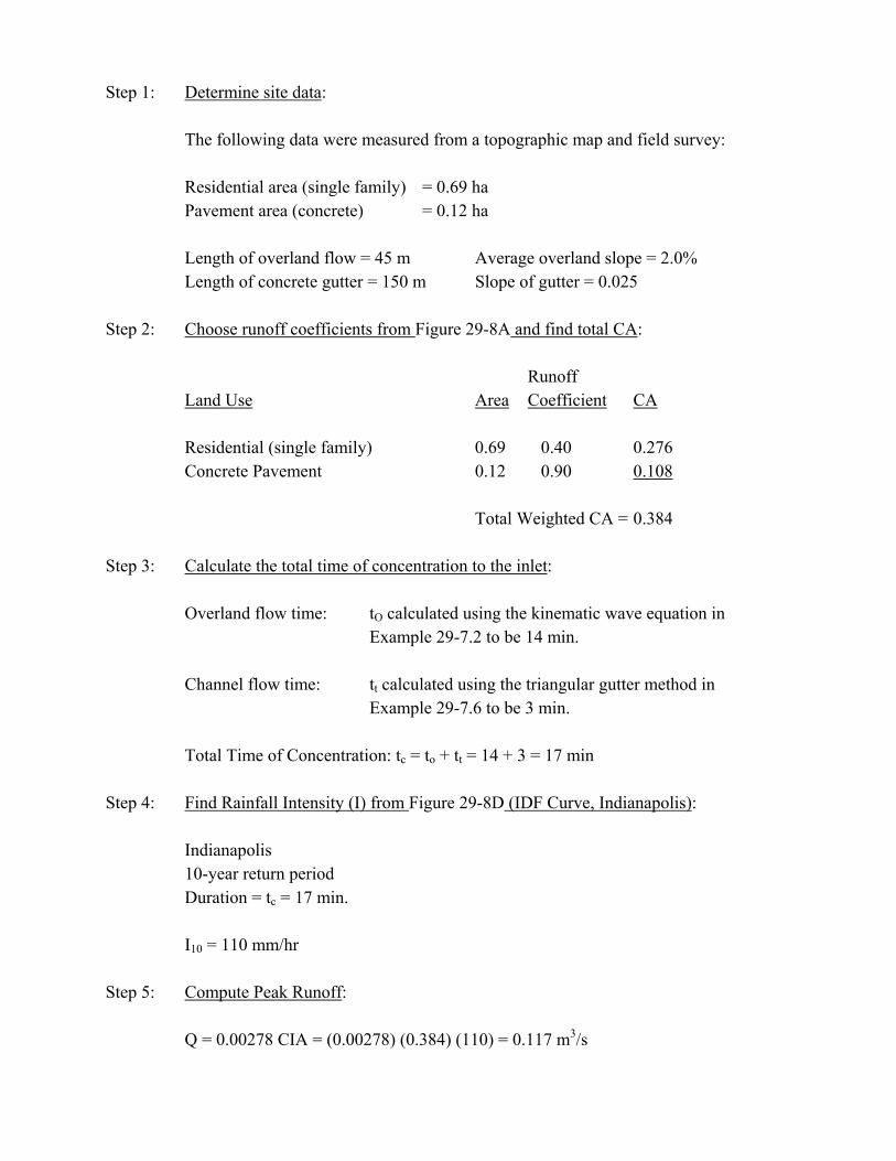
Step 1: Determine site data:

The following data were measured from a topographic map and field survey:

Residential area (single family) = 0.69 ha Pavement area (concrete) = 0.12 ha

Length of overland flow = 45 m Average overland slope = 2.0% Length of concrete gutter = 150 m Slope of gutter = 0.025

Step 2: Choose runoff coefficients from Figure 29-8A and find total CA:

Runoff Land Use Area Coefficient CA

Residential (single family) 0.69 0.40 0.276 Concrete Pavement 0.12 0.90 0.108

Total Weighted CA = 0.384

Step 3: Calculate the total time of concentration to the inlet:

Overland flow time: tO calculated using the kinematic wave equation in Example 29-7.2 to be 14 min.

Channel flow time: tt calculated using the triangular gutter method in

Example 29-7.6 to be 3 min.

Total Time of Concentration: tc = to + tt = 14 + 3 = 17 min Step 4: Find Rainfall Intensity (I) from Figure 29-8D (IDF Curve, Indianapolis):

Indianapolis 10-year return period Duration = tc = 17 min.

I10 = 110 mm/hr

Step 5: Compute Peak Runoff:

Q = 0.00278 CIA = (0.00278) (0.384) (110) = 0.117 m3/s

29-9.0 USGS REGRESSION EQUATIONS Note: As of the date of the publication of Part IV, the United States Geological Survey had not

converted its documents to the SI (metric) units of measurement. Therefore, Section 29-9.0 is presented in english units of measurement. To convert the english answer to metric, use the following equation.

/s)ft Q(in 70.02831684 = /s)m Q(in 33

Note that the USGS procedure cannot be used for final design.

29-9.01 Introduction This Section presents equations for estimating the magnitude and frequency of floods at ungaged sites on regulated and rural streams in Indiana. They are based on the USGS publication Techniques for Estimating Magnitude and Frequency of Floods on Streams in Indiana (Water-Resources Investigations Report 84-4134). The equations were developed by multiple-regression analysis of basin characteristics and peak-flow statistical data from 242 gaged locations in Indiana, Ohio and Illinois. The State of Indiana was divided into seven areas on the basis of the regression analysis. A set of equations for estimating peak discharges with recurrence intervals of 2, 10, 25, 50 and 100 years was developed for each area. Significant basin characteristics in the equations are drainage area, channel length, channel slope, mean annual precipitation, storage, precipitation intensity and a runoff coefficient. Standard errors of estimate for the equations range from 24 percent to 45 percent. This Section also presents methods for estimating flood magnitude and frequency at sites on gaged streams. 29-9.02 Hydrologic Regions Regression analyses use stream gage data to define hydrologic regions. These are geographic regions which have very similar flood frequency relationships and, as such, commonly display similar characteristics. Because of the distance between stream gages, the regional boundaries cannot be considered as precise. Figure 29-9A, Areas for Selecting Flood-Frequency USGS Estimating Equations, shows the hydrologic regional boundaries for Indiana.

Problems related to hydrologic boundaries may occur in selecting the appropriate regression equation. The watershed of interest may lie partially within two or more hydrologic regions, or it may lie totally within a hydrologic region but close to a hydrologic region boundary. In these instances, the user must exercise care in using regression equations. A field visit is recommended to first collect all available historical flood data and to compare the project watershed characteristics with those of the abutting hydrologic regions. 29-9.03 Basin Characteristics Significant basin characteristics that are required to use the USGS equations are defined as follows: 1. Design Discharge (Qt), Cubic Feet/Second (cfs). The peak discharge in cfs for the

specified design flood frequency, t. 2. Drainage Area (DA), Square Miles. The area contributing directly to runoff at the study

site. Draw outline of drainage areas on topographic map and planimeter to find area. 3. Main-Channel Slope (SL), feet per mile. The slope of the streambed between points that

are 10% and 85% of the distance from the location on the stream to the basin divide. Determine from topographic maps to nearest 0.1 ft/mi.

4. Channel Length (L), miles. The distance measured along the main channel from the

location on the stream to the basin divide is determined from topographic maps to the nearest 0.1 mile.

5. Storage (STOR), percent. The percentage of drainage area covered by lakes, ponds and

wetlands. 6. Mean Annual Precipitation (PREC), inches. The 1941-1970 average annual precipitation

is determined from Figure 29-9B, Mean Annual Precipitation (1941-1970), (Stewart, 1983). A constant of 30 inches is subtracted from the characteristics PREC for use in the estimating equations. Plot the basin centroid in Figure 29-9B and determine mean annual precipitation for that point by interpolating between lines of equal precipitation.

7. Precipitation Intensity (I24,2), inches. The maximum 24-hour precipitation having a

recurrence interval of 2 years is determined from Figure 29-9C, Two-Year, 24-Hour Projection, (Hershfield, 1961).

8. Runoff Coefficient (RC). A coefficient that relates storm runoff to soil permeability by major hydrologic soil groups is determined from Figure 29-9D, Major Hydrologic Soil Groups, (Davis, 1975). Values range from 0.3 for hydrologic soil group A to 1.0 for hydrologic soil group E.

29-9.04 Regression Equations for Ungaged Sites Figure 29-9E, Production Equations, Standard Errors of the Estimate (SEE) and Equivalent Years of Record (EY), presents the equations for ungaged sites for each of the seven geographic areas in Indiana (see Figure 29-9A). Figure 29-9F, Ranges of Area Basin Characteristics for USGS Regression Equations, presents the ranges for application of each basin characteristic to each of the geographic areas within Indiana. 29-9.05 Procedure Follow this procedure for the USGS Method: Step 1: From Figure 29-9A, locate the area of the State for the site. Step 2: From pp. 12-13 Figure 1 and pp. 71-103 Table 4 in Techniques for Estimating

Magnitude and Frequency of Floods on Streams in Indiana, USGS Report 84-4134, determine if the study site is at a gaged site or on a gaged stream.

Step 3: If the site is on a gaged stream, go to Step 6. Step 4: Determine the basin characteristics necessary to solve the regression equation

from Figure 29-9E (Prediction Equations). Step 5: Use the appropriate equation from Figure 29-9E (Prediction Equations) to solve

for the required discharges. Step 6: If the site is at a gaged location, the weighted estimate of Qt from Table 4 in the

USGS Report should be used. Step 7: If the drainage area of an ungaged site on a gaged stream is less than 50% or

greater than 150% of the drainage area of a gaged site on the same stream, the discharge should be estimated from the appropriate equation in Figure 29-9E (Prediction Equations) as if the site were on an ungaged stream. Go to Step 4.

Step 8: If the drainage area of an ungaged site on a gaged stream is between 50% and 150% of the drainage area of a gaged site on the same stream, the discharge should be an estimate calculated from both gaged data (USGS Table 4) and estimating equations (Figure 29-9E, Prediction Equations). An estimate of the process is as follows:

a. Compute the ratio:

site) (gaged QTR

site) (gaged QTW = R

Where: QTW = weighted estimate of T-year flood QTR = regression equation estimate of T-year flood Both can be obtained from Table 4 in the USGS Report

b. Compute weighting factor:

1) - (R AG

A 2 - R = R W∆

Where: R = ratio defined in Step 8a

�A = absolute value of the difference between the drainage

areas (DA) of gaged and ungaged sites

AG = DA of gaged site

c. Compute T-year peak discharge at the ungaged site by:

QT = QTR (ungaged site) x RW

Where: QTR (ungaged site) = regression equation estimate of T-year flood at ungaged site

Step 9: Convert to metric: Q(in m3/s) = 0.028316847 Q(in ft3/s)

* * * * * * * * * * Example 29-9.1 (Ungaged Stream) Given: Location: Brown County, Indiana

DA = 6.94 mi2 (ungaged site) L = 4.40 mi

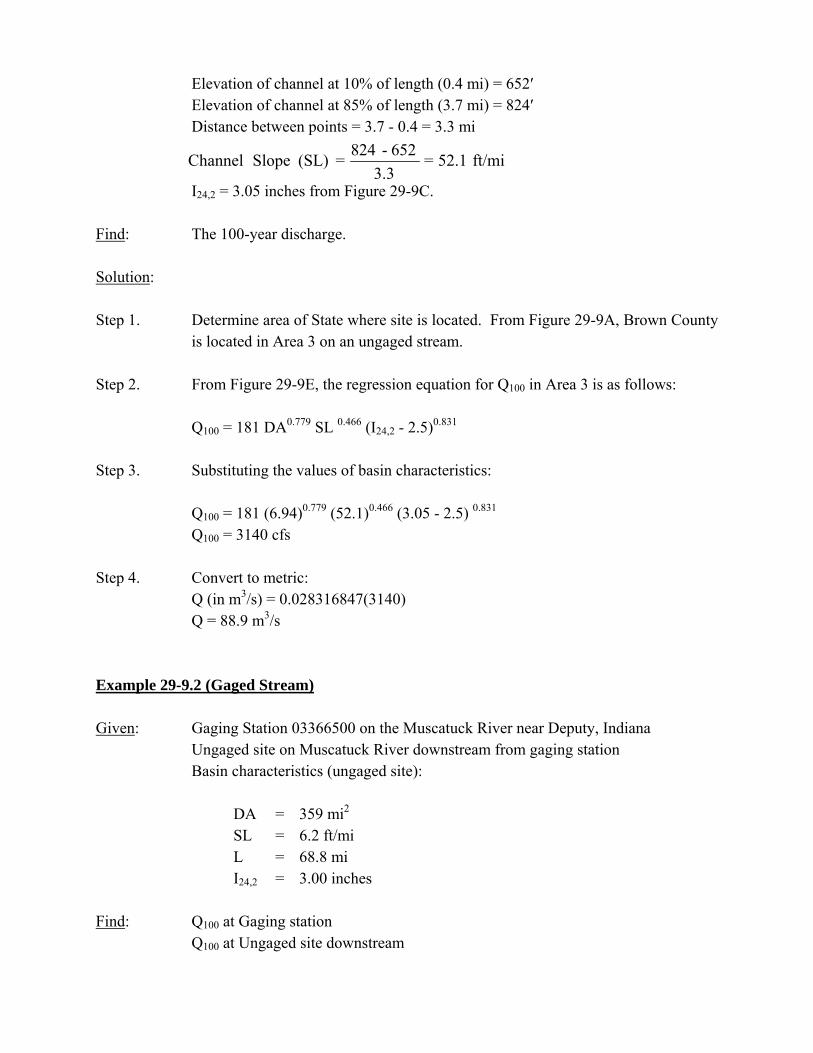
Elevation of channel at 10% of length (0.4 mi) = 652′ Elevation of channel at 85% of length (3.7 mi) = 824′ Distance between points = 3.7 - 0.4 = 3.3 mi

ft/mi 52.1 =

3.3652 - 824 = (SL) Slope Channel

I24,2 = 3.05 inches from Figure 29-9C. Find: The 100-year discharge. Solution: Step 1. Determine area of State where site is located. From Figure 29-9A, Brown County

is located in Area 3 on an ungaged stream. Step 2. From Figure 29-9E, the regression equation for Q100 in Area 3 is as follows:

Q100 = 181 DA0.779 SL 0.466 (I24,2 - 2.5)0.831 Step 3. Substituting the values of basin characteristics:

Q100 = 181 (6.94)0.779 (52.1)0.466 (3.05 - 2.5) 0.831 Q100 = 3140 cfs

Step 4. Convert to metric:

Q (in m3/s) = 0.028316847(3140) Q = 88.9 m3/s

Example 29-9.2 (Gaged Stream) Given: Gaging Station 03366500 on the Muscatuck River near Deputy, Indiana

Ungaged site on Muscatuck River downstream from gaging station Basin characteristics (ungaged site):

DA = 359 mi2

SL = 6.2 ft/mi L = 68.8 mi I24,2 = 3.00 inches

Find: Q100 at Gaging station

Q100 at Ungaged site downstream

Solution: Step 1: From Table 4 in the USGS Report, three values are given for Q100:

a. 40,900 cfs - Flood frequency analysis of observed station data b. 44,600 cfs - Regression equation c. 41,200 cfs - Weighting the station and area estimates

Select the weighted value as the best estimate:

Q100 = 41,200 cfs at gaging site

Step 2: From Figure 1 in the USGS Report and Figure 29-9A, the gaging station is located in Area 4. The regression equation for Q100 in Area 4 is:

Q100 = 32.0 DA0.565 SL0.705 L 0.730 (I24,2 - 2.5)0.464

Step 3: Substituting the values of basin characteristics:

Q100 = 32.0(359)0.565 (6.2)0.705 (68.8)0.730 (3.00 - 2.5)0.464 Q100 = 51,200 cfs

ok 1.5 < and 0.5 > 1.22 = 293359 =

DA G

Step 4: Compute:

DA u Step 5: Compute the ratio:

site) (gaged QTR

site) (gaged QTW = R

0.924 = 44,60041,200 = R

Step 6: Compute weighting factor:

( )12−

∆−= R

AARR

GW

0.958 = 1) - (0.924 293

293) - (359 2 - 0.924 = R W

Step 7: Reduce regression value by weighting factor:

QT = 51,200 x 0.958 = 49,000 cfs Step 9: Convert to metric:

Q (in m3/s) = 0.028316847(49,000) Q = 1387.5 m3/s

29-10.0 NRCS UNIT HYDROGRAPH 29-10.01 Introduction Techniques developed by the US Natural Resources Conservation Service (formerly the Soil Conservation Service) for calculating rates of runoff require the same basic data as the Rational Method - drainage area, a runoff factor, time of concentration and rainfall. The NRCS approach, however, is more sophisticated because it considers also the time distribution of the rainfall, the initial rainfall losses to interception and depression storage, and an infiltration rate that decreases during the course of a storm. With the NRCS method, the direct runoff can be calculated for any storm, either real or fabricated, by subtracting infiltration and other losses from the rainfall to obtain the precipitation excess. Details of the methodology can be found in the NRCS National Engineering Handbook, Section 4. 29-10.02 Application Two types of hydrographs are used in the NRCS procedure unit hydrographs and dimensionless unit hydrographs. A unit hydrograph represents the time distribution of flow resulting from 1 mm of direct runoff occurring over the watershed in a specified time. A dimensionless hydrograph represents the composite of many unit hydrographs. The dimensionless unit hydrograph is plotted in nondimensional units of time versus time to peak and discharge at any time versus peak discharge.

Characteristics of the dimensionless hydrograph vary with the size, shape and slope of the tributary drainage area. The most significant characteristics affecting the dimensionless hydrograph shape are the basin lag and the peak discharge for a given rainfall. Basin lag is the time from the center of mass of rainfall excess to the hydrograph peak. Steep slopes, a compact shape and an efficient drainage network tend to make lag time short and peaks high; flat slopes, an elongated shape and an inefficient drainage network tend to make lag time long and peaks low.

29-10.03 Equations and Concepts The following discussion outlines the equations and basic concepts utilized in the NRCS method. 1. Drainage Area. The drainage area of a watershed is determined from topographic maps

and field surveys. For large drainage areas it might be necessary to divide the area into subdrainage areas to account for major land use changes, obtain analysis results at different points within the drainage area, or locate stormwater drainage facilities and assess their effects on the flood flows. Also a field inspection of existing or proposed drainage systems should be made to determine if the natural drainage divides have been altered. These alterations could make significant changes in the size and slope of the subdrainage areas.

2. Rainfall. See Figure 29-10A, Huff Distribution of Design Rainfall (50% Probability of

Design Rainfall). Quartile II is recommended for use. The rainfall intensity for the given duration and return period should be multiplied by the duration to determine rainfall depth in millimeters.

3. Rainfall-Runoff Equation. A relationship between accumulated rainfall and

accumulated runoff has been derived by NRCS from experimental plots for numerous soils and vegetative cover conditions. Data for land-treatment measures, such as contouring and terracing, from experimental watersheds have been included. Equation 29-10.1 was developed mainly for small watersheds for which only daily rainfall and watershed data are ordinarily available. It was developed from recorded storm data that included total amount of rainfall in a calendar day but not its distribution with respect to time. The NRCS runoff equation is therefore a method of estimating direct runoff from 24-hr or 1-day storm rainfall. The equation is as follows:

Q = (P - Ia)2 / (P - Ia) + S (Equation 29-10.1)

Where: Q = accumulated direct runoff, mm

P = accumulated rainfall (potential maximum runoff), mm

Ia = initial abstraction including surface storage, interception and

infiltration prior to runoff, mm

S = potential maximum retention, mm

The relationship between Ia and S was developed from experimental watershed data. It removes the necessity for estimating Ia for common usage. The empirical relationship used in the NRCS runoff equation is as follows:

Ia = 0.2S (Equation 29-10.2) Substituting 0.2S for Ia in Equation 29-10.1, the NRCS rainfall-runoff equation becomes:

Q = (P - 0.2S)2 / (P + 0.8S) (Equation 29-10.3) Figure 29-10B, NCRS Relation Between Direct Runoff, Curve Number and Precipitation, shows a graphical solution of Equation 29-10.3 which enables the precipitation excess from a storm to be obtained if the total rainfall and watershed curve number are known. 29-10.04 Procedure Following is a discussion of procedures that are used in the hydrograph method and recommended tables and figures.

29-10.04(01) Runoff Factor In hydrograph applications, runoff is often referred to as rainfall excess or effective rainfall all defined as the amount by which rainfall exceeds the capability of the land to infiltrate or otherwise retain the rain water. The principal physical watershed characteristics affecting the relationship between rainfall and runoff are land use, land treatment, soil types and land slope. Land use is the watershed cover, and it includes both agricultural and nonagricultural uses. Items such as type of vegetation, water surfaces, roads, roofs, etc., are all part of the land use. Land treatment applies mainly to agricultural land use, and it includes mechanical practices such as contouring or terracing and management practices such as rotation of crops. The NRCS uses a combination of soil conditions and land-use (ground cover) to assign a runoff factor to an area. These runoff factors, called runoff curve numbers (CN), indicate the runoff potential of an area when the soil is not frozen. The higher the CN, the higher the runoff potential.

Soil properties influence the relationship between rainfall and runoff by affecting the rate of infiltration. The NRCS has divided soils into four hydrologic soil groups based on infiltration rates (Groups A, B, C and D). These groups were previously described for the Rational Method. The applicable NRCS soil classification maps may be obtained from the appropriate county agencies. Consideration should be given to the effects of urbanization on the natural hydrologic soil group. If heavy equipment can be expected to compact the soil during construction or if grading will mix the surface and subsurface soils, appropriate changes should be made in the soil group selected. Also, runoff curve numbers vary with the antecedent soil moisture conditions, defined as the amount of rainfall occurring in a selected period preceding a given storm. In general, the greater the antecedent rainfall, the more direct runoff there is from a given storm. A 5-day period is used as the minimum for estimating antecedent moisture conditions. Antecedent soil moisture conditions also vary during a storm; heavy rain falling on a dry soil can change the soil moisture condition from dry to average to wet during the storm period. The following figures provide a series of runoff factors. Figures 29-10C provides runoff curve numbers for urban areas, Figure 29-10D provides those for undeveloped areas, and Figure 29-10E provides those for agricultural lands. These tables are based on an average antecedent moisture condition; i.e., soils that are neither very wet nor very dry when the design storm begins. Curve numbers should be selected only after a field inspection of the watershed and a review of zoning and soil maps. Figure 29-10F provides conversion from average antecedent moisture conditions. Figure 29-10G provides rainfall groups for antecedent soil moisture conditions during growing and dormant seasons.

29-10.04(02) Time of Concentration The average slope within the watershed together with the overall length and retardance of overland flow are the major factors affecting the runoff rate through the watershed. In the NRCS method, time of concentration (tC) is defined to be the time required for water to travel from the most hydraulically distant point in a watershed to its outlet. Lag (L) can be considered as a weighted time of concentration and is related to the physical properties of a watershed, such as area, length and slope. The NRCS derived the following empirical relationship between lag and time of concentration.

L = 0.6 tC (Equation 29-10.4) In small urban areas (less than 810 ha), a curve number method can be used to estimate the time of concentration from watershed lag. In this method, the lag for the runoff from an increment of

excess rainfall can be considered as the time between the center of mass of the excess rainfall increment and the peak of its incremental outflow hydrograph. The equation developed by NRCS to estimate lag is:

L = (l0.8 (S/2.54 + 1)0.7) / (735 Y0.5) (Equation 29-10.5) Where: L = lag, hr

l = length of mainstream to farthest divide, m Y = average slope of watershed, % S = 25.4 [(1000/CN) - 10], mm CN = NRCS curve number

The lag time can be corrected for the effects of urbanization by using Figure 29-10H, Factors for Adjusting Lag (When Impervious Areas Occur in Watershed), and Figure 29-10 I, Factors for Adjusting Lag (When Main Channel Has Been Hydraulically Improved). The amount of modifications to the hydraulic flow length usually must be determined from topographic maps or aerial photographs following a field inspection of the area. The modification to the hydraulic flow length not only includes pipes and channels but also the length of flow in streets and driveways. After the lag time is adjusted for the effects of urbanization, Equation 29-10.4 that relates lag time and time of concentration can be used to calculate the time of concentration for use in the NRCS method. Section 29-7.0 presents an alternative procedure for travel time and time of concentration estimation.

29-10.04(03) Triangular Hydrograph Equation The triangular hydrograph is a practical representation of excess runoff with only one rise, one peak and one recession. Its geometric configuration can be easily described mathematically, which makes it very useful in estimating discharge rates. The NRCS developed Equation 29-10.6 to estimate the peak rate of discharge for an increment of runoff.

qp = (0.208 A (q)) / (d/2 + L) (Equation 29-10.6)

Where: qp = peak rate of discharge, m3/s A = area, km2 q = storm runoff during time interval, mm d = time interval, hr L = watershed lag, hr

Equation 29-10.6 can be used to estimate the peak discharge for the unit hydrograph which can then be used to estimate the peak discharge and hydrograph from the entire watershed. The constant 0.208, or peak rate factor, is valid for the NRCS dimensionless unit hydrograph. Any change in the dimensionless unit hydrograph reflecting a change in the percent of volume under the rising side will cause a corresponding change in the shape factor associated with the triangular hydrograph and therefore a change in the constant 0.208. This constant has been known to vary from about 0.258 in steep terrain to 0.129 in very flat swampy country. 29-10.05 TR-20 Example Problem (NRCS Method) The Natural Resources Conservation Service developed the computerized program TR-20 to perform the calculations for the NRCS hydrologic methodology. Note that the program is in the inch-pound units of measurement, and all input and output data must be in English. To run TR-20, the user must input the following data: 1. desired design frequency, 2. runoff Curve Number, 3. average watershed slope, 4. stream cross section data, 5. reach length, 6. structure data, 7. cumulative rainfall table (including desired time increment), 8. antecedent moisture condition, 9. storm characteristics, 10. routing instructions, and 11. desired output. The following pages provide a sample output from TR-20.

29-11.0 HEC 1 HEC 1 was developed by the US Army Corps of Engineers in 1967. It is also a hydrograph-oriented program with the capability to compute, combine and route hydrographs through a system of subareas. HEC 1 can be utilized for any basin size, and there is no lower limit on basin size. Input requirements are similar to TR-20. A detailed description of HEC 1 is not presented in Chapter Twenty-nine because of is similarities to TR-20.

29-12.0 REFERENCES 1. AASHTO Highway Drainage Guidelines, Volume II. 2. Federal Highway Administration, HYDRAIN Documentation, 1990. 3. USGS, Water-Resources Investigations Report 84-4134 Techniques For Estimating

Magnitude and Frequency of Floods on Streams in Indiana. 4. AASHTO Model Drainage Manual, 1991 and 1997. 5. Indiana DNR, Coordinated Discharges of Selected Streams in Indiana. 6. U.S. Department of Transportation, Federal Highway Administration, Hydrology, 1994.

Hydraulic Engineering Circular No. 19. 7. Water Resources Council Bulletin 17B Guidelines for Determining Flood Flow

Frequency, 1981. 8. Storm Water Drainage Manual, Highway Extension and Research Project for Indiana

Counties and Cities, H-94-6, July 1994. 9. Hydrology and Hydraulics in Indiana, Volume 1, Indiana Department of Natural

Resources, Division of Water, January 1986.